FAME: Feature-Based Adversarial Meta-Embeddings
for Robust Input Representations

Abstract

Combining several embeddings typically improves performance in downstream tasks as different embeddings encode different information. It has been shown that even models using embeddings from transformers still benefit from the inclusion of standard word embeddings. However, the combination of embeddings of different types and dimensions is challenging. As an alternative to attention-based meta-embeddings, we propose feature-based adversarial meta-embeddings (FAME) with an attention function that is guided by features reflecting word-specific properties, such as shape and frequency, and show that this is beneficial to handle subword-based embeddings. In addition, FAME uses adversarial training to optimize the mappings of differently-sized embeddings to the same space. We demonstrate that FAME works effectively across languages and domains for sequence labeling and sentence classification, in particular in low-resource settings. FAME sets the new state of the art for POS tagging in 27 languages, various NER settings and question classification in different domains.

1 Introduction

Recent work on word embeddings and pre-trained language models has shown the large impact of language representations on natural language processing (NLP) models across tasks and domains Devlin et al. (2019); Beltagy et al. (2019); Conneau et al. (2020). Nowadays, a large number of different embedding models are available with different characteristics, such as different input granularities (word-based (e.g., Mikolov et al., 2013; Pennington et al., 2014) vs. subword-based (e.g., Heinzerling and Strube, 2018; Devlin et al., 2019) vs. character-based (e.g., Lample et al., 2016; Ma and Hovy, 2016; Peters et al., 2018)), or different data used for pre-training (general-world vs. specific domain). Since those characteristics directly influence when embeddings are most effective, combinations of different embedding models are likely to be beneficial Tsuboi (2014); Kiela et al. (2018); Lange et al. (2019b), even when using already powerful large-scale pre-trained language models Akbik et al. (2018); Yu et al. (2020). Word-based embeddings, for instance, are strong in modeling frequent words while character-based embeddings can model out-of-vocabulary words. Similarly, domain-specific embeddings can capture in-domain words that do not appear in general domains like news text.

Different word representations can be combined using so-called meta-embeddings. There are several methods available, ranging from concatenation (e.g., Yin and Schütze, 2016), over averaging (e.g., Coates and Bollegala, 2018) to attention-based meta-embeddings Kiela et al. (2018). However, they all come with shortcomings: Concatenation leads to high-dimensional input vectors and, as a result, requires additional parameters in the first layer of the neural network. Averaging simply merges all information into one vector, not allowing the network to focus on specific embedding types which might be more effective than others to represent the current word. Attention-based embeddings address this problem by allowing dynamic combinations of embeddings depending on the current input token. However, the calculation of attention weights requires the model to assess the quality of embeddings for a specific word. This is arguably very challenging when embeddings of different input granularities are combined, e.g., subwords and words. Infrequent in-domain tokens, for instance, are hard to detect when using subword-based embeddings as they can model any token. Moreover, both average and attention-based meta-embeddings require a mapping of all embeddings into the same space which can be challenging for a set of embeddings with different dimensions.

In this paper, we propose feature-based adversarial meta-embeddings (FAME) that (1) align the embedding spaces with adversarial training, and (2) use attention for combining embeddings with a layer that is guided by features reflecting word-specific properties, such as the shape or frequency of the word and, thus, can help the model to assess the quality of the different embeddings. By using attention, we avoid the shortcomings of concatenation (high-dimensional input vectors) and averaging (merging information without focus). Further, our contributions mitigate the challenges of previous attention-based meta-embeddings: In our analysis, we show that the first contribution is especially beneficial when embeddings of different dimensions are combined. The second helps, in particular, when combining word-based with subword-based embeddings.

We conduct experiments across a variety of tasks, languages and domains, including sequence-labeling tasks (named entity recognition (NER) for four languages, concept extraction for two special domains (clinical and materials science), and part-of-speech tagging (POS) for 27 languages) and sentence classification tasks (question classification in different domains). Our results and analyses show that FAME outperforms existing meta-embedding methods and that even powerful fine-tuned transformer models can benefit from additional embeddings using our method. In particular, FAME sets the new state of the art for POS tagging in all 27 languages, for NER in two languages, as well as on all tested concept extraction and two question classification datasets.

In summary, our contributions are meta-embeddings with (i) adversarial training and (ii) a feature-based attention function. (iii) We perform broad experiments, ablation studies and analyses which demonstrate that our method is highly effective across tasks, domains and languages, including low-resource settings. (iv) Moreover, we show that even representations from large-scale pre-trained transformer models can benefit from our meta-embeddings approach. The code for FAME is publicly available and compatible with the flair framework Akbik et al. (2018).

2 Related Work

This section surveys related work on meta-embeddings, attention and adversarial training.

Meta-Embeddings. Previous work has seen performance gains by, for example, combining various types of word embeddings Tsuboi (2014) or the same type trained on different corpora Luo et al. (2014). For the combination, some alternatives have been proposed, such as different input channels of a convolutional neural network Kim (2014); Zhang et al. (2016), concatenation followed by dimensionality reduction Yin and Schütze (2016) or averaging of embeddings Coates and Bollegala (2018), e.g., for combining embeddings from multiple languages  Lange et al. (2020b); Reid et al. (2020). More recently, auto-encoders Bollegala and Bao (2018); Wu et al. (2020), ensembles of sentence encoders Poerner et al. (2020) and attention-based methods Kiela et al. (2018); Lange et al. (2019a) have been introduced. The latter allows a dynamic (input-based) combination of multiple embeddings. Winata et al. (2019) and Priyadharshini et al. (2020) used similar attention functions to combine embeddings from different languages for NER in code-switching settings. Liu et al. (2021) explored the inclusion of domain-specific semantic structures to improve meta-embeddings in non-standard domains. In this paper, we follow the idea of attention-based meta-embeddings and propose task-independent methods for improving them.

Extended Attention. Attention has been introduced in the context of machine translation Bahdanau et al. (2015) and is since then widely used in NLP (i.a., Tai et al., 2015; Xu et al., 2015; Yang et al., 2016; Vaswani et al., 2017). Our approach extends this technique by integrating word features into the attention function. This is similar to extending the source of attention for uncertainty detection Adel and Schütze (2017) or relation extraction Zhang et al. (2017b); Li et al. (2019). However, in contrast to these works, we use task-independent features derived from the token itself. Thus, we can use the same attention function for different tasks.

Adversarial Training. Further, our method is motivated by the usage of adversarial training Goodfellow et al. (2014) for creating input representations that are independent of a specific domain or feature. This is related to using adversarial training for domain adaptation Ganin et al. (2016) or coping with bias or confounding variables Li et al. (2018); Raff and Sylvester (2018); Zhang et al. (2018); Barrett et al. (2019); McHardy et al. (2019). Following Ganin et al. (2016), we use gradient reversal training in this paper. Recent studies use adversarial training on the word level to enable cross-lingual transfer from a source to a target language Zhang et al. (2017a); Keung et al. (2019); Wang et al. (2019); Bari et al. (2020). In contrast, our discriminator is not binary but multinomial (as in Chen and Cardie (2018)) and allows us to create a common space for embeddings from different granularities.

3 Meta-Embeddings

In this section, we present our proposed FAME model with feature-based meta-embeddings with adversarial training. The FAME model is depicted in Figure 1.

3.1 Attention-Based Meta-Embeddings

As some embeddings are more effective in modeling certain words, e.g., domain-specific embeddings for in-domain words, we use attention-based meta-embeddings that are able to combine different embeddings dynamically as introduced by Kiela et al. (2018).

Given $n$ embeddings $e_{1}\in\mathbb{R}^{E_{1}}$, … $e_{n}\in\mathbb{R}^{E_{n}}$ of potentially different dimensions $E_{1}$, … $E_{n}$, they first need to be mapped to the same space (with $E$ dimensions): $x_{i}=\tanh(Q_{i}\cdot e_{i}+b_{i}),1\leq i\leq n$. Note that the mapping parameters $Q_{i}\in\mathbb{R}^{E\times E_{i}}$ and $b_{i}\in\mathbb{R}^{E}$ are learned for each embedding method during training of the downstream task. Then, attention weights $\alpha_{i}$ are computed by:

$$\alpha_{i}=\frac{\exp(V\cdot\tanh(Wx_{i}))}{\sum_{l=1}^{n}\exp(V\cdot\tanh(Wx_{l}))}$$ (1)

with $W\in\mathbb{R}^{H\times E}$ and $V\in\mathbb{R}^{1\times H}$ being parameter matrices that are randomly initialized and learned during training. Finally, the embeddings $x_{i}$ are weighted using the attention weights $\alpha_{i}$ resulting in the word representation:

$$e^{ATT}=\sum_{i}\alpha_{i}\cdot x_{i}$$ (2)

This approach requires the model to learn parameters for the mapping function as well as for the attention function. The first might be challenging if the original embeddings have different dimensions while the latter might be hard if the embeddings represent inputs from different granularities, such as words vs. subwords. We support this claim experimentally in our analysis in Section 6.2.

3.2 Feature-Based Attention

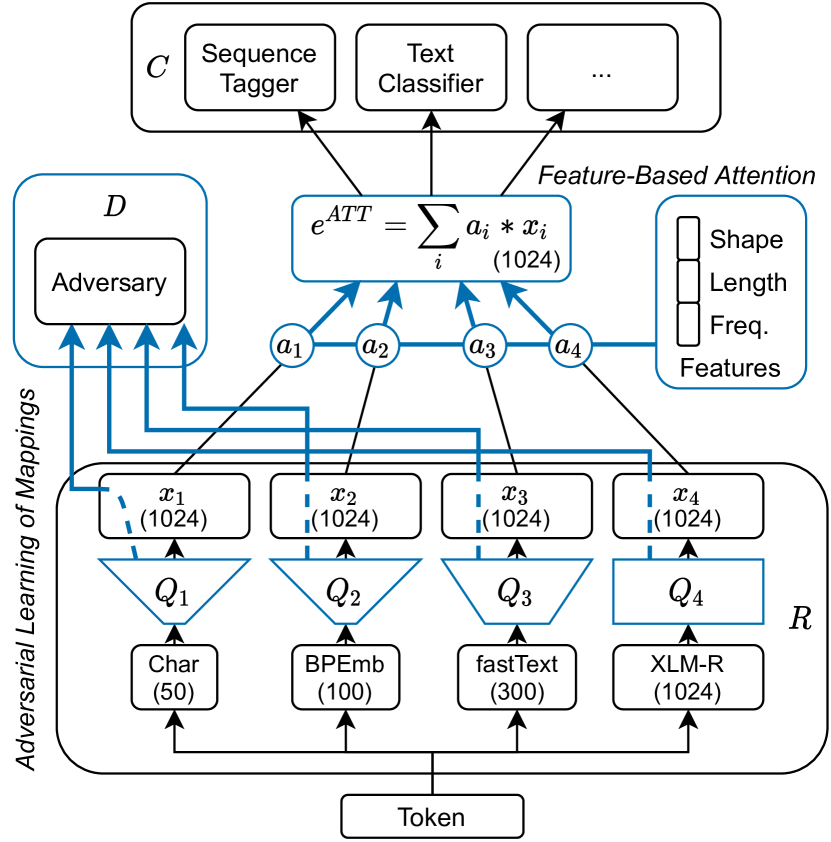
Figure 1: Overview of the FAME model architecture. Blue lines highlight our contributions. $C$ (classifier), $D$ (discriminator) and $R$ (input representation) denote the components of adversarial training. The dimensions of intermediate representations are given in parentheses.

Equation 1 for calculating attention weights only depends on $x_{i}$, the representation of the current word. While this can be enough when only standard word embeddings are used, subword- and character-based embeddings are able to create vectors for out-of-vocabulary inputs and distinguishing these from tailored vectors for frequent words is challenging without further information (see Section 6.2). To allow the model to make an informed decision which embeddings to focus on, we propose to use the features described below as an additional input to the attention function. The word features are represented as a vector $f\in\mathbb{R}^{F}$ and integrated into the attention function (Equation 1) as follows:

$$\alpha_{i}=\frac{\exp(V\cdot\tanh(Wx_{i}+Uf))}{\sum_{l=1}^{n}\exp(V\cdot\tanh(Wx_{l}+Uf))}$$ (3)

with $U\in\mathbb{R}^{H\times F}$ being a parameter matrix that is learned during training.

Features.

FAME uses the following task-independent features based on word characteristics.

- Length: Long words, in particular compounds, are often less frequent in embedding vocabularies, such that the word length can be an indicator for rare or out-of-vocabulary words. We encode the lengths in 20-dimensional one-hot vectors. Words with more than 19 characters share the same vector.

- Frequency: High-frequency words can typically be modeled well by word-based embeddings, while low-frequency words are better captured with subword-based embeddings. Moreover, frequency is domain-dependent and can thus help to decide between embeddings from different domains. We estimate the frequency $n$ of a word in the general domain from its rank $r$ in the FastText-based embeddings provided by Grave et al. (2018): $n(r)=k/r$ with $k=0.1$, following Manning and Schütze (1999). Finally, we group the words into 20 bins as in Mikolov et al. (2011) and represent their frequency with a 20-dimensional one-hot vector.

- Word Shape: Word shapes capture certain linguistic features and are often part of manually designed feature sets, e.g., for CRF classifiers Lafferty et al. (2001). For example, uncommon word shapes can be indicators for domain-specific words, which can benefit from domain-specific embeddings. We create 12 binary features that capture information on the word shape, including whether the first, any or all characters are uppercased, alphanumerical, digits or punctuation marks.

- Word Shape Embeddings: In addition, we train word shape embeddings (25 dimensions) similar to Limsopatham and Collier (2016). For this, the shape of each word is converted by replacing letters with c or C (depending on the capitalization), digits with n and punctuation marks with p. For instance, Dec. 12th would be converted to Cccp nncc. The resulting shapes are one-hot encoded and a trainable randomly initialized linear layer is used to compute the shape representation.

All sparse feature vectors (binary or one-hot encoded) are fed through a linear layer to generate a dense representation. Finally, all features are concatenated into a single feature vector $f$ of 77 dimensions which is used in the attention function as described earlier.

3.3 Adversarial Learning of Mappings

The attention-based meta-embeddings require that all embeddings have the same dimension for summation. For this, mapping matrices need to be learned, as only a limited number of embeddings exist for many languages and domains, and there is typically no option to only use embeddings of the same size. To learn an effective mapping, we propose to use adversarial training. In particular, FAME adapts gradient-reversal training with three components: the representation module $R$ consisting of the different embedding models and the mapping functions $Q$ to the common embedding space, a discriminator $D$ that tries to distinguish the different embeddings from each other, and a downstream classifier $C$ which is either a sequence tagger or a sentence classifier in our experiments (and is described in more detail in Section 4).

The input representation is shared between the discriminator and downstream classifier and trained with gradient reversal to fool the discriminator. To be more specific, the discriminator $D$ is a multinomial non-linear classification model with a standard cross-entropy loss function $L_{D}$. In our sequence tagging experiments, the downstream classifier $C$ has a conditional random field (CRF) output layer and is trained with a CRF loss $L_{C}$ to maximize the log probability of the correct tag sequence Lample et al. (2016). In our sentence classification experiments, $C$ is a multinomial classifier with cross-entropy loss $L_{C}$. Let $\theta_{R}$, $\theta_{D}$, $\theta_{C}$ be the parameters of the representation module, discriminator and downstream classifier, respectively. Gradient reversal training will update the parameters as follows:

$$\theta_{D} =\theta_{D}-\eta\lambda\frac{\partial L_{D}}{\partial\theta_{D}};\;\;\;\theta_{C}=\theta_{C}-\eta\frac{\partial L_{C}}{\partial\theta_{C}}$$ (4)

$$\theta_{R} =\theta_{R}-\eta(\frac{\partial L_{C}}{\partial\theta_{R}}-\lambda\frac{\partial L_{D}}{\partial\theta_{R}})$$ (5)

with $\eta$ being the learning rate and $\lambda$ being a hyperparameter to control the discriminator influence.

4 Neural Architectures

In this section, we present the architectures we use for text classification and sequence tagging. Note that our contribution concerns the input representation layer, which can be used with any NLP model, e.g., also sequence-to-sequence models.

	Dimensions	Fine-tuned?
General Domain
Character	50	Yes
BPEmb	100	No
FastText	300	No
XLM-R	1024	No / Yes
Domain-specific
Word	100 (En), 300 (Es)	No
Transformer	768 (En)	No / Yes

Table 1: Overview of embeddings used in our models.

4.1 Input Layer

The input to our neural networks is our FAME meta-embeddings layer as described in Section 3. Our methodology does not depend on the embedding method, i.e., it can incorporate any token representation. In our experiments, we use the embeddings listed in Table 1 based on insights from related work. In particular, Akbik et al. (2018) showed the advantages of character and FastText embeddings Bojanowski et al. (2017) and Heinzerling and Strube (2018) showed similar results for character and BPE embeddings. Thus, we decided to use the union (char+FastText +BPE) with a state-of-the-art multilingual Transformer (Conneau et al., 2020, XLM-R). Our character-based embeddings are randomly initialized and accumulated to token embeddings using a bidirectional long short-term memory network Hochreiter and Schmidhuber (1997) with 25 hidden units in each direction.

For experiments in non-standard domains, we add domain-specific embeddings, including word embeddings from the clinical domain for English Pyysalo et al. (2013) and Spanish Gutiérrez-Fandiño et al. (2021) and the materials science domain Tshitoyan et al. (2019). Further, we include domain-specific transformer models for experiments on English data, i.e., Clinical BERT Alsentzer et al. (2019) trained on MIMIC, and SciBERT Beltagy et al. (2019) trained on academic publications from semantic scholar.

For all experiments, our baselines and proposed models use the same set of embeddings. We experiment with both freezing and fine-tuning the transformer embeddings during training. However, note that fine-tuning the transformer model increases the model size by more than a factor of 100 from 4M trainable parameters to 535M as shown in Table 2. This increases computational costs by a large margin. For example, in our experiments, the time for training a single epoch for English NER increases from 3 to 38 minutes.

	Transformer fine-tuned?
Meta-embeddings method	No	Yes
General Domain (4 embeddings)
Concatenation	10.0 / 3.4	543.9 / 539.4
Attention-based meta-emb	4.0 / 4.0	537.9 / 538.9
Feature-based attention	4.0 / 4.0	538.0 / 538.9
Domain-specific (4+2 embeddings)
Concatenation	14.9 / 5.3	652.2 / 648.2
Attention-based meta-emb	4.9 / 4.9	642.2 / 643.2
Feature-based attention	5.0 / 4.9	642.2 / 643.2
+ Adversarial Discriminator	+1.0 / +1.0	+1.0 / +1.0

Table 2: Number of trainable parameters (in million) of our models for sequence labeling / text classification.

4.2 Model for Sequence Tagging

Our sequence tagger follows a well-known architecture Lample et al. (2016) with a bidirectional long short-term memory (BiLSTM) network and conditional random field (CRF) output layer Lafferty et al. (2001). Note that we perform sequence tagging on sentence level without cross-sentence context as done, i.a., by Schweter and Akbik (2020).

4.3 Models for Text Classification

For sentence classification, we use a BiLSTM sentence encoder. The resulting sentence representation is fed into a linear layer followed by a softmax activation that outputs label probabilities.

4.4 Hyperparameters and Training

To ensure reproducibility, we describe details of our models and training procedure in the following.

Hyperparameters.

We use hidden sizes of 256 units per direction for all BiLSTMs. The attention layer has a hidden size $H$ of 10. We set the mapping size $E$ to the size of the largest embedding in all experiments, i.e., 1024 dimensions, the size of XLM-R embeddings. The discriminator $D$ has a hidden size of 1024 units and is trained every 10^th batch. We perform a hyperparameter search for the $\lambda$ parameter in {1e-4, 1e-5, 1e-6, 1e-7} for models using adversarial training. Note that we use the same hyperparameters for all models and all tasks.

Training.

We use the AdamW optimizer with an initial learning rate of 5e-6. We train the models for a maximum of 100 epochs and select the best model according to the performance using the task’s metric on the development set if available, or using the training loss otherwise. The training was performed on Nvidia Tesla V100 GPUs with 32GB VRAM.

5 Experiments and Results

We now describe the tasks and datasets we use in our experiments as well as our results.

	NER
Model	En	De	Es	Nl
Schweter and Akbik (2020)	93.69	92.29	89.93	94.66
Yu et al. (2020)	93.5	90.3	90.3	93.7
XLM-R Conneau et al. (2020)	92.92	85.81	89.72	92.53
FAME (our model)	94.11	92.28	89.90	95.42

	Concept Extraction
Model	ClinEn	ClinEs	SofcEn
Alsentzer et al. (2019)	87.7	-	-
Lange et al. (2020a)	88.9	91.4	–
Friedrich et al. (2020)	–	–	81.5
FAME (our model)	90.08	92.68	83.68

Table 3: NER and concept extraction results ($F_{1}$). XLM-R is a fine-tuned transformer Conneau et al. (2020).

5.1 Tasks and Datasets

Sequence Labeling.

For sequence labeling, we use named entity recognition (NER) and part-of-speech tagging (POS) datasets from different domains and languages. For NER, we use the CoNLL benchmark datasets from the news domain (English/German/Dutch/Spanish) Tjong Kim Sang (2002); Tjong Kim Sang and De Meulder (2003). In addition, we conduct experiments for concept extraction on two datasets from the clinical domain, the English i2b2 2010 data Uzuner et al. (2011) and the Spanish PharmaCoNER task Gonzalez-Agirre et al. (2019), as well as experiments on the materials science domain Friedrich et al. (2020). For POS tagging, we use the universal dependencies treebanks version 1.2 (UPOS tag) and use the 27 languages for which Yasunaga et al. (2018) reported numbers.

Sentence Classification.

We experiment with three question classifications tasks, namely the TREC corpus Voorhees and Tice (1999) with 6 or 50 labels and GARD (Kilicoglu et al., 2016, clinical domain).

5.2 Evaluation Results

We now present the results of our experiments. All reported numbers are the averages of three runs.

Sequence Labeling.

Tables 3 and 4 show the results for sequence labeling in comparison to the state of the art. Our models consistently set the new state of the art for English and Dutch NER, for domain-specific concept extraction as well as for all 27 languages for POS tagging. The comparison with XML-R on NER shows that our FAME method can also improve upon already powerful transformer representations. In domain-specific concept extraction, we outperform related work by 1.5 $F_{1}$-points on average. This shows that our approach works across languages and domains.

	SOTA1	SOTA2	SOTA3	FAME
Bg (Bulgarian)	97.97	98.53	98.7	99.53
Cs (Czech)	98.24	98.81	98.9	99.33
Da (Danish)	96.35	96.74	97.0	99.13
De (German)	93.38	94.35	94.0	95.95
En (English)	95.17	95.82	95.6	98.09
Es (Spanish)	95.74	96.44	96.5	97.75
Eu (Basque)	95.51	94.71	95.6	97.66
Fa (Persian)	97.49	97.51	97.1	98.68
Fi (Finnish)	95.85	95.40	94.6	98.67
Fr (French)	96.11	96.63	96.2	97.19
He (Hebrew)	96.96	97.43	96.6	98.00
Hi (Hindi)	97.10	97.21	97.0	98.35
Hr (Croatian)	96.82	96.32	96.8	97.96
Id (Indonesian)	93.41	94.03	93.4	94.24
It (Italian)	97.95	98.08	98.1	98.82
Nl (Dutch)	93.30	93.09	93.8	94.74
No (Norwegian)	98.03	98.08	98.1	99.16
Pl (Polish)	97.62	97.57	97.5	99.05
Pt (Portuguese)	97.90	98.07	98.2	98.86
Sl (Slovenian)	96.84	98.11	98.0	99.44
Sv (Swedish)	96.69	96.70	97.3	99.17
Avg.	96.40	96.65	96.6	98.08
El (Greek)	-	98.24	97.9	98.89
Et (Estonian)	-	91.32	92.8	97.07
Ga (Irish)	-	91.11	91.0	94.27
Hu (Hungarian)	-	94.02	94.0	97.72
Ro (Romanian)	-	91.46	89.7	96.64
Ta (Tamil)	-	83.16	88.7	91.10
Avg.	-	91.55	92.4	95.95

Table 4: POS tagging results (accuracy) (using gold segmentation). SOTA1 refers to results from Plank et al. (2016), SOTA2 to Yasunaga et al. (2018) and SOTA3 to Heinzerling and Strube (2019). As Yasunaga et al. (2018), we split into high-resource (top) and low-resource languages (bottom).

	corresponding to	NER				Concept Extraction			POS (subset)
Model	baseline meta-emb.	En	De	Es	Nl	ClinEn	ClinEs	SofcEn	Et	Ga	Ta
FAME (our model, w/ fine-tuning)		94.11	92.28	89.90	95.42	90.08	92.68	83.68	97.07	94.27	91.10
FAME (our model, w/o fine-tuning)		93.43	91.96	88.86	93.28	89.23	91.97	81.85	96.03	91.47	89.58
– features		93.37	91.66	88.37	92.98	89.07	91.42	81.48	95.81	90.20	88.73
– adversarial	Attention (ATT)	93.22	91.52	88.16	92.46	88.87	91.33	81.31	95.19	87.79	87.93
– attention	Average (AVG)	92.38	90.14	88.44	92.37	88.69	90.23	80.28	93.20	86.95	87.73
– sum, mapping	Concatenation (CAT)	91.00	90.54	85.40	88.51	87.97	90.66	80.08	91.63	86.32	84.51

Table 5: Ablation study results for sequence labeling. We underline our FAME models without fine-tuning for which we found statistically significant differences to the attention-based meta-embeddings (ATT).

Model	TREC-6	TREC-50	GARD
Xu et al. (2020)	96.2	92.0	84.9
Roberts et al. (2014)	-	-	80.4
Xia et al. (2018)	98.0	-	-
FAME (our model)	98.2	93.0	87.90

Table 6: Sentence classification results (accuracy).

Sentence Classification.

Similar to sequence labeling, our FAME approach outperforms the existing machine learning models on all three tested sentence classification datasets as shown in Table 6. This demonstrates that our approach is generally applicable and can be used for different tasks beyond the token level.

6 Analysis

We finally analyze the different components of our proposed FAME model by investigating, i.a., ablation studies, attention weights and low-resource settings.

6.1 Ablation Study on Model Components

Table 5 provides an ablation study on the different components of our FAME model for exemplary sequence-labeling tasks.

First, we ablate the fine-tuning of the embedding models as we found that this has a large impact on the number of parameters of our models (538M vs. 4M) and, as a result, on the training time (cf., Section 4.1). Our results show that fine-tuning does have a positive impact on the performance of our models but our approach still works very well with frozen embeddings. In particular, our non-finetuned FAME model is competitive to a finetuned XLM-R model (see Table 3) and outperforms it on 3 out of 4 languages for NER.

Second, we ablate our two newly introduced components (features and adversarial training) and find that both of them have a positive impact on the performance of our models across tasks, languages and domains.

With successively removing components, we obtain models that actually correspond to baseline meta-embeddings as shown in the second column of the table. Our method without features and adversarial training, for example, corresponds to the baseline attention-based meta-embedding approach (ATT). Further removing the attention function yields average-based meta-embeddings (AVG). Finally, we also evaluate another baseline meta-embedding alternative, namely concatenation (CAT). Note that concatenation leads to a very high-dimensional input representation and, therefore, requires more parameters in the next neural network layer, which can be inefficient in practice.

Statistical Significance. To show that FAME significantly improves upon the attention-based meta-embeddings, we report statistical significance between those two models (using our method without fine-tuning for a fair comparison). Table 5 shows that we find statistically significant differences in six out of ten settings.

6.2 Influence of Embedding Granularities and Dimensions

Next, we perform an analysis to show the effects of our method for embeddings of different dimensions and granularities and support our motivation that our contributions help in those settings. As a testbed, we perform Spanish concept extraction and utilize the embeddings published by Grave et al. (2018) and Gutiérrez-Fandiño et al. (2021) as they allow us to nicely isolate the desired effects.

In particular, they published pairs of embeddings (all having 300 dimensions) that were trained on the same corpora. The first embeddings are standard word embeddings and the second embeddings are subword embeddings with out-of-vocabulary functionality. As both were trained on the same data, we can isolate the effect of embedding granularities in a first experiment. In addition, Gutiérrez-Fandiño et al. (2021) published smaller versions with 100 dimensions that were trained under the same conditions. We use those in a second experiment to analyze the effects of combining embeddings of different dimensions.

The results are shown in Table 7. We find that adversarial training becomes particularly important whenever differently-sized embeddings are combined, i.e., when the model needs to learn mappings to higher dimensions.

Further, we see that the inclusion of our proposed features helps substantially in the presence of subword embeddings. The reason might be that with sets of both word-based and subword-based embeddings, it gets harder to decide which embeddings are useful (e.g., word-based embeddings for high-frequency words) and should, thus, get higher attention weights. Our features have been designed in a way to explicitly guide the attention function in those cases, e.g., by indicating the frequency of a word. In addition, Table 8 shows an ablation study on our different features for this testbed setting. We see that length and shape are the most important features, as excluding either of them reduces performance the most.

Dim.	Same		Different
Gran.	Word	Subword	Word	Subword
ATT	89.27	88.00	88.60	88.16
+ FEAT	89.28 (+.01)	88.62 (+.62)	88.64 (+.04)	88.42 (+.26)
+ ADV	89.34 (+.07)	88.31 (+.31)	89.23 (+.63)	88.44 (+.28)

Table 7: Effect of our proposed methods on embeddings of different granularities (word vs. subword) and dimensions (same vs. different dim.). ATT: attention-based meta-embeddings, FEAT: feature-based attention function, ADV: adversarial training of mapping. We add the differences between our methods and ATT.

Attention function	$F_{1}$	($\Delta$)
no features	88.0
all features	88.62	(+.62)
– shape	88.65	(+.65)
– frequency	88.61	(+.61)
– length	88.45	(+.45)
– shape embedding	88.34	(+.34)

Table 8: Ablation Study: Features.

6.3 Training in Low-Resource Settings

As we observed large positive effects of our method for low-resource languages (Table 4), we now perform a study to further investigate this topic. We simulate low-resource scenarios by artificially limiting the training data of the CoNLL NER corpora to different percentages of all instances. The results are visualized in Figure 2. We find that the differences between the standard attention-based meta-embeddings (ATT) and our FAME method get larger with fewer training samples, with up to 6.7 $F_{1}$ points for English when 5% of the training data is used, which corresponds to roughly 600 labeled sentences. This behavior holds for all four languages and highlights the advantages of our method when only limited training data is available. An interesting future research direction is the exploration of FAME for real-world low-resource domains and languages Hedderich et al. (2021).

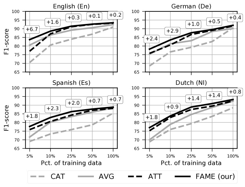
Figure 2: Performance for different training set sizes. The highlighted numbers display the difference between our FAME model without fine-tuning and the attention-based meta-embeddings (ATT). Further, we compare to the baseline methods averaging (AVG) and concatenation (CAT) of embeddings.

6.4 Analysis of Embedding Methods

We studied the performance of each embedding method in isolation. The results are shown in Table 9 and indicate that FastText and XLM-R embeddings are the best options in this setting. This observation is also reflected in the attention weights assigned by the FAME model (see Figure 4). In general, FastText and XLM-R embeddings get assigned the highest weights. This highlights that the attention-based meta-embeddings are able to perform a suitable embedding selection and reduce the need for manual feature selection.

The combination of all four embeddings is better than every single embedding, which shows the importance of combining different embeddings. In particular, the FAME model outperforms concatenation by a large margin regardless if the transformer embedding is fine-tuned.

	Input Dim.	NewsEn $F_{1}$
Single embeddings
Character	50	77.02
BPEmb	100	86.37
FastText	300	90.45
XLM-R	1024	89.23
All embeddings
CAT	1474	91.0
FAME	1024	93.43
Fine-tuned transformer
XLM-R	1024	92.12
CAT	1474	92.75
FAME	1024	94.11

Table 9: Overview of embeddings used in our models.

6.5 Analysis of Attention Weights

Figure 3 provides the change of attention weights from the average for the domain-specific embeddings for a sentence from the clinical domain. It shows that the attention weights for the clinical embeddings are higher for in-domain words, such as “mg”, “PRN” (which stands for “pro re nata”) or “PO” (which refers to “per os”) and lower for general-domain words, such as “every”, “6” or “hours”. Thus, FAME is able to recognize the value of domain-specific embeddings in non-standard domains and assigns attention weights accordingly.

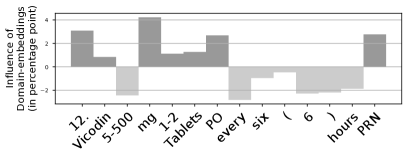
Figure 3: Changes in influence of domain-specific embeddings on meta-embeddings. The model prefers domain-specific embeddings for in-domain words.

Figure 4 shows how attention weights change for frequency and length features as introduced in Section 3.2. In particular, it demonstrates that subword-based embeddings (BPEmb and XLM-R) get more important for long and infrequent words which are usually not well covered in the fixed vocabulary of standard word embeddings.

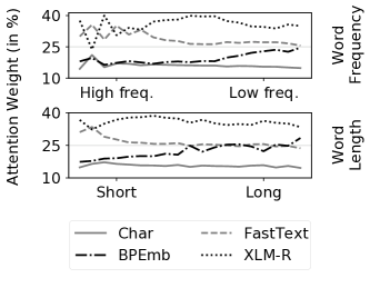
Figure 4: Attention weights assigned by the FAME model for the Clin_En corpus grouped by the features word frequency (above) and length (below).

6.6 Analysis of Adversarial Training

In contrast to previous work Lange et al. (2020c), we show that adversarial training is also beneficial and boosts performance in a monolingual case when combining multiple embeddings. The embeddings were trained independent from each other. Thus, the individual embedding spaces are clearly separated. Adversarial training shifts all embeddings closer to a common space as shown in Figure 5, which is important if the average is taken for the attention-based meta-embeddings approach.

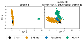
Figure 5: The meta-embeddings space before (left) and after NER and adversarial training (right).

7 Conclusions

In this paper, we proposed feature-based adversarial meta-embeddings (FAME) to effectively combine several embeddings. The features are designed to guide the attention layer when computing the attention weights, in particular for embeddings representing different input granularities, such as subwords or words. Adversarial training helps to learn better mappings when embeddings of different dimensions are combined. We demonstrate the effectiveness of our approach on a variety of sentence classification and sequence tagging tasks across languages and domains and set the new state of the art for POS tagging in 27 languages, for domain-specific concept extraction on three datasets, for NER in two languages, as well as on two question classification datasets. Further, our analysis shows that our approach is particularly successful in low-resource settings. A future direction is the evaluation of our method on sequence-to-sequence tasks or document representations.

References

- Adel and Schütze (2017) Heike Adel and Hinrich Schütze. 2017. Exploring different dimensions of attention for uncertainty detection. In Proceedings of the 15th Conference of the European Chapter of the Association for Computational Linguistics: Volume 1, Long Papers, pages 22–34, Valencia, Spain. Association for Computational Linguistics.
- Akbik et al. (2018) Alan Akbik, Duncan Blythe, and Roland Vollgraf. 2018. Contextual string embeddings for sequence labeling. In Proceedings of the 27th International Conference on Computational Linguistics, pages 1638–1649, Santa Fe, New Mexico, USA. Association for Computational Linguistics.
- Alsentzer et al. (2019) Emily Alsentzer, John Murphy, William Boag, Wei-Hung Weng, Di Jindi, Tristan Naumann, and Matthew McDermott. 2019. Publicly available clinical BERT embeddings. In Proceedings of the 2nd Clinical Natural Language Processing Workshop, pages 72–78, Minneapolis, Minnesota, USA. Association for Computational Linguistics.
- Bahdanau et al. (2015) Dzmitry Bahdanau, Kyunghyun Cho, and Yoshua Bengio. 2015. Neural machine translation by jointly learning to align and translate. In 3rd International Conference on Learning Representations, ICLR 2015, San Diego, CA, USA, May 7-9, 2015, Conference Track Proceedings.
- Bari et al. (2020) M. Saiful Bari, Shafiq Joty, and Prathyusha Jwalapuram. 2020. Zero-resource cross-lingual named entity recognition. In Proceedings of the 34th AAAI Conference on Artificial Intelligence (AAAI 2020), pages 7415–7423.
- Barrett et al. (2019) Maria Barrett, Yova Kementchedjhieva, Yanai Elazar, Desmond Elliott, and Anders Søgaard. 2019. Adversarial removal of demographic attributes revisited. In Proceedings of the 2019 Conference on Empirical Methods in Natural Language Processing and the 9th International Joint Conference on Natural Language Processing (EMNLP-IJCNLP), pages 6329–6334, Hong Kong, China. Association for Computational Linguistics.
- Beltagy et al. (2019) Iz Beltagy, Kyle Lo, and Arman Cohan. 2019. SciBERT: A pretrained language model for scientific text. In Proceedings of the 2019 Conference on Empirical Methods in Natural Language Processing and the 9th International Joint Conference on Natural Language Processing (EMNLP-IJCNLP), pages 3615–3620, Hong Kong, China. Association for Computational Linguistics.
- Bojanowski et al. (2017) Piotr Bojanowski, Edouard Grave, Armand Joulin, and Tomas Mikolov. 2017. Enriching word vectors with subword information. Transactions of the Association for Computational Linguistics, 5:135–146.
- Bollegala and Bao (2018) Danushka Bollegala and Cong Bao. 2018. Learning word meta-embeddings by autoencoding. In Proceedings of the 27th International Conference on Computational Linguistics, pages 1650–1661, Santa Fe, New Mexico, USA. Association for Computational Linguistics.
- Chen and Cardie (2018) Xilun Chen and Claire Cardie. 2018. Multinomial adversarial networks for multi-domain text classification. In Proceedings of the 2018 Conference of the North American Chapter of the Association for Computational Linguistics: Human Language Technologies, Volume 1 (Long Papers), pages 1226–1240, New Orleans, Louisiana. Association for Computational Linguistics.
- Coates and Bollegala (2018) Joshua Coates and Danushka Bollegala. 2018. Frustratingly easy meta-embedding – computing meta-embeddings by averaging source word embeddings. In Proceedings of the 2018 Conference of the North American Chapter of the Association for Computational Linguistics: Human Language Technologies, Volume 2 (Short Papers), pages 194–198, New Orleans, Louisiana. Association for Computational Linguistics.
- Conneau et al. (2020) Alexis Conneau, Kartikay Khandelwal, Naman Goyal, Vishrav Chaudhary, Guillaume Wenzek, Francisco Guzmán, Edouard Grave, Myle Ott, Luke Zettlemoyer, and Veselin Stoyanov. 2020. Unsupervised cross-lingual representation learning at scale. In Proceedings of the 58th Annual Meeting of the Association for Computational Linguistics, pages 8440–8451, Online. Association for Computational Linguistics.
- Devlin et al. (2019) Jacob Devlin, Ming-Wei Chang, Kenton Lee, and Kristina Toutanova. 2019. BERT: Pre-training of deep bidirectional transformers for language understanding. In Proceedings of the 2019 Conference of the North American Chapter of the Association for Computational Linguistics: Human Language Technologies, Volume 1 (Long and Short Papers), pages 4171–4186, Minneapolis, Minnesota. Association for Computational Linguistics.
- Friedrich et al. (2020) Annemarie Friedrich, Heike Adel, Federico Tomazic, Johannes Hingerl, Renou Benteau, Anika Marusczyk, and Lukas Lange. 2020. The SOFC-exp corpus and neural approaches to information extraction in the materials science domain. In Proceedings of the 58th Annual Meeting of the Association for Computational Linguistics, pages 1255–1268, Online. Association for Computational Linguistics.
- Ganin et al. (2016) Yaroslav Ganin, Evgeniya Ustinova, Hana Ajakan, Pascal Germain, Hugo Larochelle, François Laviolette, Mario Marchand, and Victor Lempitsky. 2016. Domain-adversarial training of neural networks. J. Mach. Learn. Res., 17(1):2096–2030.
- Gonzalez-Agirre et al. (2019) Aitor Gonzalez-Agirre, Montserrat Marimon, Ander Intxaurrondo, Obdulia Rabal, Marta Villegas, and Martin Krallinger. 2019. PharmaCoNER: Pharmacological substances, compounds and proteins named entity recognition track. In Proceedings of The 5th Workshop on BioNLP Open Shared Tasks, pages 1–10, Hong Kong, China. Association for Computational Linguistics.
- Goodfellow et al. (2014) Ian Goodfellow, Jean Pouget-Abadie, Mehdi Mirza, Bing Xu, David Warde-Farley, Sherjil Ozair, Aaron Courville, and Yoshua Bengio. 2014. Generative adversarial nets. In Advances in Neural Information Processing Systems 27, pages 2672–2680. Curran Associates, Inc.
- Grave et al. (2018) Edouard Grave, Piotr Bojanowski, Prakhar Gupta, Armand Joulin, and Tomas Mikolov. 2018. Learning word vectors for 157 languages. In Proceedings of the Eleventh International Conference on Language Resources and Evaluation (LREC 2018), Miyazaki, Japan. European Language Resources Association (ELRA).
- Gutiérrez-Fandiño et al. (2021) Asier Gutiérrez-Fandiño, Jordi Armengol-Estapé, Casimiro Pio Carrino, Ona De Gibert, Aitor Gonzalez-Agirre, and Marta Villegas. 2021. Spanish biomedical and clinical language embeddings. arXiv preprint arXiv:2102.12843.
- Hedderich et al. (2021) Michael A. Hedderich, Lukas Lange, Heike Adel, Jannik Strötgen, and Dietrich Klakow. 2021. A survey on recent approaches for natural language processing in low-resource scenarios. In Proceedings of the 2021 Conference of the North American Chapter of the Association for Computational Linguistics: Human Language Technologies, pages 2545–2568, Online. Association for Computational Linguistics.
- Heinzerling and Strube (2018) Benjamin Heinzerling and Michael Strube. 2018. BPEmb: Tokenization-free pre-trained subword embeddings in 275 languages. In Proceedings of the Eleventh International Conference on Language Resources and Evaluation (LREC 2018), Miyazaki, Japan. European Language Resources Association (ELRA).
- Heinzerling and Strube (2019) Benjamin Heinzerling and Michael Strube. 2019. Sequence tagging with contextual and non-contextual subword representations: A multilingual evaluation. In Proceedings of the 57th Annual Meeting of the Association for Computational Linguistics, pages 273–291, Florence, Italy. Association for Computational Linguistics.
- Hochreiter and Schmidhuber (1997) Sepp Hochreiter and Jürgen Schmidhuber. 1997. Long short-term memory. Neural Computation, 9(8):1735–1780.
- Keung et al. (2019) Phillip Keung, Yichao Lu, and Vikas Bhardwaj. 2019. Adversarial learning with contextual embeddings for zero-resource cross-lingual classification and NER. In Proceedings of the 2019 Conference on Empirical Methods in Natural Language Processing and the 9th International Joint Conference on Natural Language Processing (EMNLP-IJCNLP), pages 1355–1360, Hong Kong, China. Association for Computational Linguistics.
- Kiela et al. (2018) Douwe Kiela, Changhan Wang, and Kyunghyun Cho. 2018. Dynamic meta-embeddings for improved sentence representations. In Proceedings of the 2018 Conference on Empirical Methods in Natural Language Processing, pages 1466–1477, Brussels, Belgium. Association for Computational Linguistics.
- Kilicoglu et al. (2016) Halil Kilicoglu, Asma Ben Abacha, Yassine Mrabet, Kirk Roberts, Laritza Rodriguez, Sonya Shooshan, and Dina Demner-Fushman. 2016. Annotating named entities in consumer health questions. In Proceedings of the Tenth International Conference on Language Resources and Evaluation (LREC’16), pages 3325–3332, Portorož, Slovenia. European Language Resources Association (ELRA).
- Kim (2014) Yoon Kim. 2014. Convolutional neural networks for sentence classification. In Proceedings of the 2014 Conference on Empirical Methods in Natural Language Processing (EMNLP), pages 1746–1751, Doha, Qatar. Association for Computational Linguistics.
- Lafferty et al. (2001) John D. Lafferty, Andrew McCallum, and Fernando C. N. Pereira. 2001. Conditional random fields: Probabilistic models for segmenting and labeling sequence data. In Proceedings of the Eighteenth International Conference on Machine Learning, ICML ’01, pages 282–289, San Francisco, CA, USA. Morgan Kaufmann Publishers Inc.
- Lample et al. (2016) Guillaume Lample, Miguel Ballesteros, Sandeep Subramanian, Kazuya Kawakami, and Chris Dyer. 2016. Neural architectures for named entity recognition. In Proceedings of the 2016 Conference of the North American Chapter of the Association for Computational Linguistics: Human Language Technologies, pages 260–270, San Diego, California. Association for Computational Linguistics.
- Lange et al. (2019a) Lukas Lange, Heike Adel, and Jannik Strötgen. 2019a. NLNDE: Enhancing neural sequence taggers with attention and noisy channel for robust pharmacological entity detection. In Proceedings of The 5th Workshop on BioNLP Open Shared Tasks, pages 26–32, Hong Kong, China. Association for Computational Linguistics.
- Lange et al. (2019b) Lukas Lange, Heike Adel, and Jannik Strötgen. 2019b. NLNDE: The neither-language-nor-domain-experts’ way of spanish medical document de-identification. In Proceedings of The Iberian Languages Evaluation Forum (IberLEF 2019), CEUR Workshop Proceedings.
- Lange et al. (2020a) Lukas Lange, Heike Adel, and Jannik Strötgen. 2020a. Closing the gap: Joint de-identification and concept extraction in the clinical domain. In Proceedings of the 58th Annual Meeting of the Association for Computational Linguistics, pages 6945–6952, Online. Association for Computational Linguistics.
- Lange et al. (2020b) Lukas Lange, Heike Adel, and Jannik Strötgen. 2020b. On the choice of auxiliary languages for improved sequence tagging. In Proceedings of the 5th Workshop on Representation Learning for NLP, pages 95–102, Online. Association for Computational Linguistics.
- Lange et al. (2020c) Lukas Lange, Anastasiia Iurshina, Heike Adel, and Jannik Strötgen. 2020c. Adversarial alignment of multilingual models for extracting temporal expressions from text. In Proceedings of the 5th Workshop on Representation Learning for NLP, pages 103–109, Online. Association for Computational Linguistics.
- Li et al. (2019) Pengfei Li, Kezhi Mao, Xuefeng Yang, and Qi Li. 2019. Improving relation extraction with knowledge-attention. In Proceedings of the 2019 Conference on Empirical Methods in Natural Language Processing and the 9th International Joint Conference on Natural Language Processing (EMNLP-IJCNLP), pages 229–239, Hong Kong, China. Association for Computational Linguistics.
- Li et al. (2018) Yitong Li, Timothy Baldwin, and Trevor Cohn. 2018. Towards robust and privacy-preserving text representations. In Proceedings of the 56th Annual Meeting of the Association for Computational Linguistics (Volume 2: Short Papers), pages 25–30, Melbourne, Australia. Association for Computational Linguistics.
- Limsopatham and Collier (2016) Nut Limsopatham and Nigel Collier. 2016. Bidirectional LSTM for named entity recognition in twitter messages. In Proceedings of the 2nd Workshop on Noisy User-generated Text (WNUT), pages 145–152, Osaka, Japan. The COLING 2016 Organizing Committee.
- Liu et al. (2021) Qian Liu, Jie Lu, Guangquan Zhang, Tao Shen, Zhihan Zhang, and Heyan Huang. 2021. Domain-specific meta-embedding with latent semantic structures. Information Sciences, 555:410–423.
- Luo et al. (2014) Yong Luo, Jian Tang, Jun Yan, Chao Xu, and Zheng Chen. 2014. Pre-trained multi-view word embedding using two-side neural network. In Proceedings of the 28th AAAI Conference on Artificial Intelligence (AAAI 2014), pages 1982–1988.
- Ma and Hovy (2016) Xuezhe Ma and Eduard Hovy. 2016. End-to-end sequence labeling via bi-directional LSTM-CNNs-CRF. In Proceedings of the 54th Annual Meeting of the Association for Computational Linguistics (Volume 1: Long Papers), pages 1064–1074, Berlin, Germany. Association for Computational Linguistics.
- Manning and Schütze (1999) Christopher D. Manning and Hinrich Schütze. 1999. Foundations of Statistical Natural Language Processing. MIT Press, Cambridge, MA, USA.
- McHardy et al. (2019) Robert McHardy, Heike Adel, and Roman Klinger. 2019. Adversarial training for satire detection: Controlling for confounding variables. In Proceedings of the 2019 Conference of the North American Chapter of the Association for Computational Linguistics: Human Language Technologies, Volume 1 (Long and Short Papers), pages 660–665, Minneapolis, Minnesota. Association for Computational Linguistics.
- Mikolov et al. (2011) Tomas Mikolov, Stefan Kombrink, Lukas Burget, Jan Černocký, and Sanjeev Khudanpur. 2011. Extensions of recurrent neural network language model. In 2011 IEEE International Conference on Acoustics, Speech and Signal Processing (ICASSP), pages 5528–5531.
- Mikolov et al. (2013) Tomas Mikolov, Ilya Sutskever, Kai Chen, Greg Corrado, and Jeffrey Dean. 2013. Distributed representations of words and phrases and their compositionality. In Proceedings of the 26th International Conference on Neural Information Processing Systems - Volume 2, NIPS’13, pages 3111–3119, USA. Curran Associates Inc.
- Pennington et al. (2014) Jeffrey Pennington, Richard Socher, and Christopher Manning. 2014. Glove: Global vectors for word representation. In Proceedings of the 2014 Conference on Empirical Methods in Natural Language Processing (EMNLP), pages 1532–1543, Doha, Qatar. Association for Computational Linguistics.
- Peters et al. (2018) Matthew Peters, Mark Neumann, Mohit Iyyer, Matt Gardner, Christopher Clark, Kenton Lee, and Luke Zettlemoyer. 2018. Deep contextualized word representations. In Proceedings of the 2018 Conference of the North American Chapter of the Association for Computational Linguistics: Human Language Technologies, Volume 1 (Long Papers), pages 2227–2237, New Orleans, Louisiana. Association for Computational Linguistics.
- Plank et al. (2016) Barbara Plank, Anders Søgaard, and Yoav Goldberg. 2016. Multilingual part-of-speech tagging with bidirectional long short-term memory models and auxiliary loss. In Proceedings of the 54th Annual Meeting of the Association for Computational Linguistics (Volume 2: Short Papers), pages 412–418, Berlin, Germany. Association for Computational Linguistics.
- Poerner et al. (2020) Nina Poerner, Ulli Waltinger, and Hinrich Schütze. 2020. Sentence meta-embeddings for unsupervised semantic textual similarity. In Proceedings of the 58th Annual Meeting of the Association for Computational Linguistics, pages 7027–7034, Online. Association for Computational Linguistics.
- Priyadharshini et al. (2020) Ruba Priyadharshini, Bharathi R. Chakravarthi, Mani Vegupatti, and John P. McCrae. 2020. Named entity recognition for code-mixed indian corpus using meta embedding. In Proceedings of the 2020 6th International Conference on Advanced Computing and Communication Systems (ICACCS), pages 68–72, Coimbatore, India. IEEE.
- Pyysalo et al. (2013) Sampo Pyysalo, Filip Gintern, Hans Moen, Tapio Salakoski, and Sophia Ananiadou. 2013. Distributional semantics resources for biomedical text processing. Proceedings of the Second International Symposium on Languages in Biology and Medicine (LBM) 2007, pages 39–44.
- Raff and Sylvester (2018) Edward Raff and Jared Sylvester. 2018. Gradient reversal against discrimination: A fair neural network learning approach. In 2018 IEEE 5th International Conference on Data Science and Advanced Analytics (DSAA), pages 189–198.
- Reid et al. (2020) Machel Reid, Edison Marrese-Taylor, and Yutaka Matsuo. 2020. Combining pretrained high-resource embeddings and subword representations for low-resource languages. CoRR, abs/2003.04419.
- Roberts et al. (2014) Kirk Roberts, Halil Kilicoglu, Marcelo Fiszman, and Dina Demner-Fushman. 2014. Automatically classifying question types for consumer health questions. In AMIA Annual Symposium Proceedings, volume 2014, page 1018. American Medical Informatics Association.