Random hyperbolic graphs in $d+1$ dimensions

Abstract

We consider random hyperbolic graphs in hyperbolic spaces of any dimension $d+1\geq 2$. We present a rescaling of model parameters that casts the random hyperbolic graph model of any dimension to a unified mathematical framework, leaving the degree distribution invariant with respect to $d$. We analyze the limiting regimes of the model, and release a software package that generates random hyperbolic graphs and their limits in hyperbolic spaces of any dimension.

I Introduction

Random hyperbolic graphs (RHGs) Krioukov et al. (2009, 2010) are a latent space network model McFarland and Brown (1973); Hoff et al. (2002), in which the latent space is the hyperbolic plane $\mathbb{H}^{2}$: nodes are random points on the plane, while connections between nodes are established with distance-dependent probabilities. RHGs reproduce many structural properties of real networks including sparsity, self-similarity, power-law degree distribution, strong clustering, small worldness, and community structure Serrano et al. (2008); Krioukov et al. (2010); Papadopoulos et al. (2012); Zuev et al. (2015); Zheng et al. (2021). Using the RHG model as a null model, one can map real networks to hyperbolic spaces Boguñá et al. (2010); Kitsak et al. (2020); García-Pérez et al. (2019), the applications of which include routing and navigation Boguñá et al. (2010, 2008); Gulyás et al. (2015); Voitalov et al. (2017); Ortiz et al. (2017); García-Pérez et al. (2018); Muscoloni and Cannistraci (2019), link prediction Serrano et al. (2012); Papadopoulos et al. (2015a, b); Muscoloni et al. (2017); Muscoloni and Cannistraci (2018a, b); García-Pérez et al. (2020); Kitsak et al. (2020), network scaling Serrano et al. (2008); García-Pérez et al. (2018); Zheng et al. (2021), semantic analysis Nickel and Kiela (2017, 2018); Dhingra et al. (2018); Tifrea et al. (2019), and many others Boguñá et al. (2021).

Here, we consider the RHG model in hyperbolic spaces $\mathbb{H}^{d+1}$ of any dimension $d+1\geq 2$, Section II. We present a rescaling of model parameters that renders the degree distribution invariant with respect to $d$, Section III, focusing on the three connectivity regimes—cold, critical, and hot—in the model, Section IV. In Section V, we analyze the limiting regimes of the model when its parameters tend to their extreme values. Section VI changes the focus from the model perspective to the random graph ensemble perspective, and presents the RHG model in terms of network property parameters. Section VII introduces our software package that generates RHGs and their limits for any $d$, generalizing the $d=1$ generator in Aldecoa et al. (2015). The concluding remarks are in Section VIII.

In comparison to existing work on the subject, RHGs are equivalent to geometric inhomogeneous random graphs (GIRGs), as mentioned in Krioukov et al. (2010) and formalized in Bringmann et al. (2019). This GIRG formulation is followed in Boguñá et al. (2020), where the small-world and clustering properties are analyzed for any dimension $d$, while Yang and Rideout (2020) adheres to the hyperbolic formulation and contains a more detailed analysis of the degree distribution and degree correlations in the model. Recently, the related popularity-similarity optimization (PSO) model has been extended to arbitrary dimensionality $d+1\geq 2$ in Kovács et al. (2022). Whereas RHGs are a static network model, the $(d+1)$-dimensional PSO model is a growing network model in hyperbolic space that achieves similar structural properties. A notable difference is that the PSO model can produce power-law degree distributions with exponent smaller than 2 in the case $d+1>2$, corresponding to extremely fat tails in the distribution. Unlike RHGs, however, it is not possible to define a specific density of radial coordinates other than the imposed logarithmically increasing sequence in the PSO model.

II Random Hyperbolic Graph Model in $d+1$ dimensions

Consider the upper sheet of the $(d+1)$-dimensional hyperboloid of curvature $K=-\zeta^{2}$

$$x_{0}^{2}-x_{1}^{2}-...-x_{d+1}^{2}=\frac{1}{\zeta^{2}},~{}x_{0}>0,$$ (1)

in the $(d+2)$-dimensional Minkowski space with metric

$${\rm d}s^{2}=-{\rm d}x_{0}^{2}+{\rm d}x_{1}^{2}+...+{\rm d}x_{d+1}^{2}.$$ (2)

The spherical coordinate system on the hyperboloid $\left(r,\theta_{1},...,\theta_{d}\right)$ is defined by

$$x_{0}= \frac{1}{\zeta}\cosh\zeta r,$$

$$x_{1}= \frac{1}{\zeta}\sinh\zeta r\cos\theta_{1},$$

$$x_{2}= \frac{1}{\zeta}\sinh\zeta r\sin\theta_{1}\cos\theta_{2},$$ (3)

$$\vdots$$

$$x_{d}= \frac{1}{\zeta}\sinh\zeta r\sin\theta_{1}...\sin\theta_{d-1}\cos\theta_{d},$$

$$x_{d+1}= \frac{1}{\zeta}\sinh\zeta r\sin\theta_{1}...\sin\theta_{d-1}\sin\theta_{d},$$

where $r>0$ is the radial coordinate and $\left(\theta_{1},...,\theta_{d}\right)$ are the standard angular coordinates on the unit $d$-dimensional sphere $\mathbb{S}^{d}$.

The coordinate transformation in (II) yields the spherical coordinate metric in the $(d+1)$-dimensional hyperbolic space $\mathbb{H}^{d+1}$

$${\rm d}s^{2} ={\rm d}r^{2}+{1\over\zeta^{2}}\sinh^{2}\left({\zeta r}\right){\rm d}\Omega_{d}^{2},$$ (4)

$${\rm d}\Omega_{d}^{2} ={\rm d}\theta_{1}^{2}+{\rm sin}^{2}(\theta_{1}){\rm d}\theta_{2}^{2}+\dots$$

$$\quad+{\rm sin}^{2}(\theta_{1})\dots\rm sin^{2}(\theta_{d-1}){\rm d}\theta_{d}^{2},$$ (5)

resulting in the volume element in $\mathbb{H}^{d+1}$:

$${\rm d}V=\left({\frac{1}{\zeta}}\sinh{\zeta r}\right)^{d}{\rm d}r\prod_{k=1}^{d}\sin^{d-k}(\theta_{k}){\rm d}\theta_{k}.$$ (6)

The distance between two points $i$ and $j$ in $\mathbb{H}^{d+1}$ is given by the hyperbolic law of cosines:

$$\cosh\zeta d_{ij}=\cosh\zeta r_{i}\cosh\zeta r_{j}-\sinh\zeta r_{i}\sinh\zeta r_{j}\cos\Delta\theta_{ij},\\$$ (7)

where $\Delta\theta_{ij}$ is the angle between $i$ and $j$:

$$\cos(\Delta\theta_{ij})=\cos\theta_{i,1}\cos\theta_{j,1}$$

$$+ \sin\theta_{i,1}\sin\theta_{j,1}\cos\theta_{i,2}\cos\theta_{j,2}+...$$

$$+ \sin\theta_{i,1}\sin\theta_{j,1}...\sin\theta_{i,d-1}\sin\theta_{j,d-1}\cos\theta_{i,d}\cos\theta_{j,d}$$

$$+ \sin\theta_{i,1}\sin\theta_{j,1}...\sin\theta_{i,d-1}\sin\theta_{j,d-1}\sin\theta_{i,d}\sin\theta_{j,d},$$ (8)

$\left(\theta_{i,1},...,\theta_{i,d}\right)$ and $\left(\theta_{j,1},...,\theta_{j,d}\right)$ are the coordinates of points $i$ and $j$ on $\mathbb{S}^{d}$.

For sufficiently large $\zeta r_{i}$ and $\zeta r_{j}$ values, the hyperbolic law of cosines in Eq. (7) is closely approximated by

$$d_{ij}=r_{i}+r_{j}+{2\over\zeta}\ln\left(\sin(\Delta\theta_{ij}/2)\right).$$ (9)

The hyperbolic ball $\mathbb{B}^{d+1}$ of radius $R>0$ is defined as the set of points with

$$r\in[0,R].$$ (10)

Nodes of the RHG are points in $\mathbb{B}^{d+1}$ selected at random with density $\rho(\mathbf{x})\equiv\rho(r)\rho(\theta_{1})...\rho(\theta_{d})$, where

$$\rho(r) =\left[\sinh(\alpha r)\right]^{d}/C_{d},~{}~{}\alpha\geq\zeta/2$$ (11)

$$C_{d} \equiv\int_{0}^{R}\left[\sinh(\alpha r)\right]^{d}{\rm d}r,$$

$$\rho(\theta_{k}) =\left[{\rm sin}(\theta_{k})\right]^{d-k}/I_{d,k},\quad k=1,\ldots,d,$$

$$I_{d,k} \equiv\int_{0}^{\pi}\left[\sin(\theta)\right]^{d-k}{\rm d}\theta=\sqrt{\pi}\frac{\Gamma[\frac{d-k+1}{2}]}{\Gamma\left[1+\frac{d-k}{2}\right]},\quad k<d,$$

$$I_{d,d} \equiv 2\pi.$$

In other words, nodes are uniformly distributed on unit sphere $\mathbb{S}^{d}$ with respect to their angular coordinates. In the special case of $\alpha=\zeta$ nodes are also uniformly distributed in $\mathbb{B}^{d+1}$.

Pairs of nodes $i$ and $j$ are connected independently with connection probability

$$p_{ij}=p\left(d_{ij}\right)={1\over 1+{\rm exp}\left(\zeta\left(d_{ij}-\mu\right)/2T\right)},$$ (12)

where $\mu>0$ and $T>0$ are model parameters and $d_{ij}$ is the distance between points $i$ and $j$ in $\mathbb{B}^{d+1}$, given by Eq. (7). We refer to parameters $T$ and $\mu$ as temperature and chemical potential, respectively, using the analogy with the Fermi-Dirac statistics. We note that the factors of $2$ and $\zeta$ in Eq. (11) are to agree with the 2-dimensional RHG Krioukov et al. (2010) that corresponds to $d=1$.

Thus, the RHG is formed in a three-step network generation process:

1. Randomly select $n$ points in $\mathbb{B}^{d+1}$ with pdf $\rho(\mathbf{x})$ in Eq. (11).

2. Calculate distances in $\mathbb{B}^{d+1}$ between all $i$-$j$ node pairs using Eq. (7).

3. Connect $i$-$j$ node pairs independently at random with distance-dependent connection probabilities $p_{ij}=p\left(d_{ij}\right)$, prescribed by Eq. (12).

Taken together, RHGs in $\mathbb{B}^{d+1}$ are fully defined by $6$ parameters: properties of the hyperbolic ball, $R$ and $\zeta$; number of nodes $n$; radial component of node distribution $\alpha$; chemical potential $\mu$ and temperature $T$.

Only four parameters, however, $\left(n,\alpha,T,R\right)$ are independent. It follows from (7) that $\zeta$ is merely a rescaling parameter for distances $\{d_{ij}\}$, and can be absorbed into the radial $r$ coordinates by the appropriate rescaling. Chemical potential $\mu$ controls the expected number of links and the sparsity of resulting network models. We demonstrate below that the sparsity requirement uniquely determines $\mu$ in terms of other RHG parameters.

The RHG model is instrumental in generating synthetic graphs with desired properties. From the graph property perspective, therefore, it might be convenient to re-define the RHG in terms of its observable properties: number of nodes $n$, expected degree $\langle k\rangle$, and the scale-free degree distribution exponent $\gamma$. We demonstrate in Section VI that the RHG can be reformulated in terms of $\left(n,\gamma,T,\langle k\rangle\right)$ parameters and provide the graph property perspective summary of the RHG model in Fig. 12.

III Degree distribution in the RHG

The structural properties of the RHG can be computed with the hidden variable formalism, Ref. Boguñá and Pastor-Satorras (2003), by treating node coordinates as hidden variables.

We begin by calculating the expected degree of node $l$ located at point $\mathbf{x_{l}}=\{r_{l},\theta_{1}^{l},...,\theta_{d}^{l}\}$:

$$\langle k(\mathbf{x_{l}})\rangle=(n-1)\int{{\rm d}\mathbf{x_{k}}\rho(\mathbf{x_{k}})\over 1+e^{\frac{\zeta\left(d_{lk}-\mu\right)}{2T}}}$$ (13)

The symmetry in the angular distribution of points ensures that the expected degree of the node depends only on its radial coordinate $r_{l}$ and not on its angular coordinates, $\langle k(\mathbf{x}_{l})\rangle=\langle k(r_{l},0,..,0)\rangle\equiv\langle k(r_{l})\rangle$. This allows us to integrate out $d$ angular coordinates in Eq. (13).

We also note that the choice of radial coordinate distribution given by Eq. (11) with $\alpha\geq\zeta/2$ results in most of the nodes having large radial coordinates, $r_{i}\approx R\gg 1$. This fact allows us to approximate distances using Eq. (9):

$$\langle k(r_{l})\rangle=\int_{0}^{R}\int_{0}^{\pi}{(n-1)\rho(r){\rm d}r\rho_{1}(\theta){\rm d}\theta\over 1+\left[e^{\zeta\left(r+r_{l}-\mu\right)}\left(\sin\left({\theta\over 2}\right)\right)^{2}\right]^{1\over 2T}}.$$ (14)

To further simplify calculations, we perform the following change of the RHG variables:

$$\{\mathfrak{r},\mathfrak{r}_{l},\mathcal{R},\mathfrak{m}\} ={d\zeta\over 2}\{r,r_{l},R,\mu\},$$ (15)

$$\tau =dT,$$

a $$=2\alpha/\zeta,$$

where the top line corresponds to $4$ equations, each corresponding to one variable in the brackets.

In terms of the rescaled variables the connection probability is

$$p_{ij}={1\over 1+e^{\frac{\mathfrak{r}_{i}+\mathfrak{r}_{j}-\mathfrak{m}}{\tau}}\left[{\rm sin}\left(\frac{\Delta\theta_{ij}}{2}\right)\right]^{\frac{d}{\tau}}},$$ (16)

while Eq. (14) reads

$$\langle k(\mathfrak{r}_{l})\rangle=\int_{0}^{\mathcal{R}}\int_{0}^{\pi}{(n-1)\rho(\mathfrak{r}){\rm d}\mathfrak{r}\rho_{1}(\theta){\rm d}\theta\over 1+e^{\frac{\mathfrak{r}+\mathfrak{r}_{l}-\mathfrak{m}}{\tau}}\left[{\rm sin}\left(\frac{\theta}{2}\right)\right]^{\frac{d}{\tau}}},$$ (17)

where

$$\rho(\mathfrak{r})\equiv\textsl{a}e^{\textsl{a}\left(\mathfrak{r}-\mathcal{R}\right)}.$$ (18)

The expected degree of the graph is given by

$$\langle k\rangle=\int_{0}^{\mathcal{R}}{\rm d}\mathfrak{r}\rho(\mathfrak{r})\langle k(\mathfrak{r})\rangle,$$ (19)

and the degree distribution of the RHG can be expressed as

$$P(k)=\int_{0}^{\mathcal{R}}{\rm d}\mathfrak{r}\rho(\mathfrak{r})P(k|\mathfrak{r}),$$ (20)

where $P(k|\mathfrak{r})$ is a conditional probability that a node with radial coordinate $\mathfrak{r}$ has exactly $k$ connections.

In the case of sparse graphs $P(k|\mathfrak{r})$ is closely approximated by the Poisson distribution:

$$P(k|\mathfrak{r})={1\over k!}e^{-\langle k(\mathfrak{r})\rangle}\left[\langle k(\mathfrak{r})\rangle\right]^{k},$$ (21)

see Ref. Boguñá and Pastor-Satorras (2003), and the resulting degree distribution $P(k)$ is a mixed Poisson distribution:

$$P(k)={1\over k!}\int_{0}^{\mathcal{R}}e^{-\langle k(\mathfrak{r})\rangle}\left[\langle k(\mathfrak{r})\rangle\right]^{k}\rho(\mathfrak{r}){\rm d}\mathfrak{r}$$ (22)

with mixing parameter $\langle k(\mathfrak{r})\rangle$.

IV Connectivity Regimes of the RHG

Depending on the value of the rescaled temperature $\tau=dT$, there exist three distinct regimes of the RHG: (i) cold regime ($\tau<1$), (ii) critical regime ($\tau=1$), and (iii) hot regime ($\tau>1$). We provide detailed analyses of the expected degree and degree distribution in these regimes below, and summarize our findings in Fig. 11.

IV.1 Cold regime, $\tau<1$

Since the inner integral in Eq. (17) does not have a closed-form solution, to estimate $\langle k(\mathfrak{r}_{l})\rangle$ we need to employ several approximations. We note that most nodes have large radial coordinates, $e^{\mathfrak{r}+\mathfrak{r}_{l}-\mathfrak{m}}\gg 1$, and the dominant contribution to the inner integral in (17) comes from small $\theta$ values. This allows us to estimate the integral by replacing $\sin(\theta)$ and $\sin(\theta/2)$ with the leading Taylor series terms, as ${\rm sin}(x)=x+\mathcal{O}\left(x^{3}\right)$, resulting in

$$\langle k(\mathfrak{r}_{l})\rangle ={(n-1)\pi^{d}\over dI_{d,1}}\int_{0}^{\mathcal{R}}{\rm d}\mathfrak{r}\rho(\mathfrak{r})~{}_{2}F_{1}\left(1,\tau,1+\tau,-u_{max}^{1\over\tau}\right),$$ (23)

$$u_{max} =\left({\pi\over 2}\right)^{d}e^{\mathfrak{r}_{l}+\mathfrak{r}-\mathfrak{m}},$$

where $~{}_{2}F_{1}$ is the Gauss hypergeometric function, and

$$I_{d,1}\equiv\int_{0}^{\pi}{\rm sin}^{d-1}(\theta){\rm d}\theta={\sqrt{\pi}\Gamma\left[{d\over 2}\right]/\Gamma\left[{d+1\over 2}\right]}$$ (24)

for $d>1$, and $I_{1,1}=2\pi$.

In the $\tau<1$ regime the hypergeometric function in (23) can be approximated as

$$~{}_{2}F_{1}\left(1,\tau,1+\tau,-u_{max}^{\frac{1}{\tau}}\right)=u_{max}^{-1}{\frac{\pi\tau}{\sin\left(\pi\tau\right)}},$$ (25)

and $\langle k(\mathfrak{r}_{l})\rangle$ and $\langle k\rangle$ are then given by:

$$\langle k\rangle =(n-1){2^{d}\over dI_{d,1}}{\pi\tau\over\sin\left(\pi\tau\right)}\langle e^{-\mathfrak{r}}\rangle^{2}e^{\mathfrak{m}},$$ (26)

$$\langle k(\mathfrak{r})\rangle ={\langle k\rangle\over\langle e^{-\mathfrak{r}}\rangle}e^{-\mathfrak{r}},$$

where $\langle e^{-\mathfrak{r}}\rangle\equiv\int_{0}^{\mathcal{R}}{\rm d}\mathfrak{r}\rho(\mathfrak{r})e^{-\mathfrak{r}}$, and the explicit expression for $\langle e^{-\mathfrak{r}}\rangle$ follows from (18):

$$\langle e^{-\mathfrak{r}}\rangle={\textsl{a}\over\textsl{a}-1}\left(e^{-\mathcal{R}}-e^{-\textsl{a}\mathcal{R}}\right).$$ (27)

We next discuss the choice of the rescaled chemical potential $\mathfrak{m}$. In order to do so, we discuss the leading order behavior of $\langle k\rangle_{n}$ in the large $n$ limit. Since $\textsl{a}>1$, we neglect the second term in (27) to obtain

$$\langle k(\mathfrak{r})\rangle_{n} \sim ne^{\mathfrak{m}-\mathfrak{r}-\mathcal{R}},$$ (28)

$$\langle k\rangle_{n} \sim ne^{\mathfrak{m}-2\mathcal{R}}.$$

Henceforth, we write $f(x)\sim g(x)$ when $\lim_{x\to\infty}\frac{f(x)}{g(x)}=K$, where $K>0$ is a constant.

We note that $\langle k(\mathfrak{r})\rangle$ decreases exponentially as a function of $\mathfrak{r}$ with the largest (smallest) expected degree corresponding to $\mathfrak{r}=0$ ($\mathfrak{r}=\mathcal{R}$). By demanding that the largest and smallest expected degrees scale as

$$\langle k_{max}\rangle_{n} = \langle k(0)\rangle_{n}\sim n,$$ (29)

$$\langle k_{min}\rangle_{n} = \langle k\left(\mathcal{R}\right)\rangle_{n}\sim 1,$$ (30)

we obtain $\mathcal{R}\sim\ln n$ and $\mathfrak{m}=\mathcal{R}+\lambda$, where $\lambda$ is an arbitrary constant.

First, we note that the scaling for $\mathcal{R}$ is consistent with our initial assumption of $\mathcal{R}\gg 1$ for large graphs. We also note that the exact value of the parameter $\lambda$ is not important as long as it is independent of $n$. To be consistent with the original $\mathbb{H}^{2}$ formulation we set $\lambda=0$, obtaining

$$\mathfrak{m}=\mathcal{R}=\ln\left(n/\nu\right),$$ (31)

where $\nu$ is the parameter controlling the expected degree of the RHG.

Applying scaling relationships (31) to (26) we obtain

$$\langle k\rangle_{n} =\nu{2^{d}\over dI_{d,1}}\left({\textsl{a}\over\textsl{a}-1}\right)^{2}{\pi\tau\over\sin(\pi\tau)}\times$$ (32)

$$\times\left[1-2\left(\frac{n}{\nu}\right)^{1-\textsl{a}}+\left(\frac{n}{\nu}\right)^{2(1-\textsl{a})}\right],$$

and

$$\langle k(\mathfrak{r})\rangle_{n}={n\over\nu}{\textsl{a}-1\over\textsl{a}}\langle k\rangle e^{-\mathfrak{r}}\sum_{\ell=0}^{\infty}\left(\frac{\nu}{n}\right)^{\ell(\textsl{a}-1)}.$$ (33)

As seen from Eq. (32) and Fig. 1, RHGs in the cold ($\tau<1$) regime are sparse. Henceforth, we call graphs sparse if their expected degree converges to a finite constant in the large graph limit. The slow convergence in the $\textsl{a}=1.1$ case to the asymptotic value of $\langle k\rangle=10$ is due to the breakdown of the ${\rm sin}(x)\approx x$ approximation in Eq. (23) for small a values. Indeed, at small a values a larger fraction of nodes is characterized by small $\mathfrak{r}$ values, for which the $e^{\left(\mathfrak{r}+\mathfrak{r}_{l}-\mathfrak{m}\right)}\gg 1$ assumption fails.

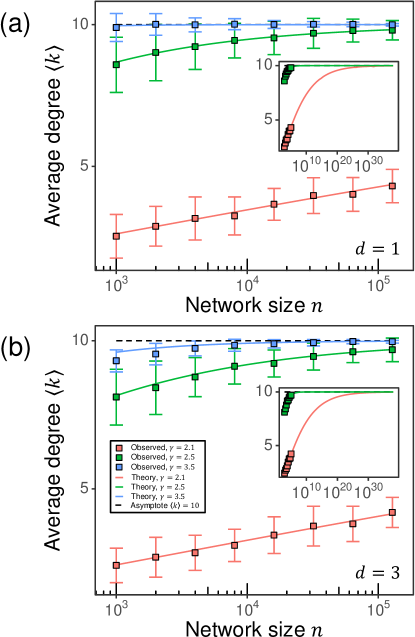
Figure 1: Expected degree $\langle k\rangle$ as a function of network size $n$ for RHGs in the cold ($\tau=0.5$) regime with (a) $d=1$ and (b) $d=3$. Each panel includes the results for (red) $\textsl{a}=1.1$ ($\gamma=2.1$), (green) $\textsl{a}=1.5$ ($\gamma=2.5$), and (blue) $\textsl{a}=2.5$ ($\gamma=3.5$). Each point is the average of $100$ simulations and the error bars display standard deviations. Solid lines are theoretical values for $\langle k\rangle$ prescribed by Eqs. (17) and (19) and the dashed line is the $n\to\infty$ limit of Eq. (32). The insets in (a) and (b) correspond to extended domains of $n$ values for the cases $\textsl{a}=1.1$ and $\textsl{a}=1.5$. Note that the $\textsl{a}=1.1$ case converges to the asymptotic value at a much slower rate compared to the $\textsl{a}=1.5$ and $\textsl{a}=2.5$ cases.

Finally, using (21) and (22) we obtain the Pareto-mixed Poisson distribution, which is a power law

$$P(k)=(\gamma-1)\kappa_{0}^{\gamma-1}{\Gamma[k-\textsl{a},\kappa_{0}]\over\Gamma[k+1]}\sim k^{-\gamma},$$ (34)

where $\Gamma[s,x]$ is the upper incomplete gamma function, $\gamma=\textsl{a}+1$, and $\kappa_{0}\equiv\frac{\gamma-2}{\gamma-1}\langle k\rangle$, as confirmed by simulations in Fig. 2.

Hence, the cold regime corresponds to sparse scale-free graphs with $\gamma\in(2,\infty)$. We note that the degree distribution is called scale-free if it takes the form of $P(k)=\ell(k)k^{-\gamma}$, where $\ell(k)$ is a slowly varying function, i.e., a function that varies slowly at infinity, see Ref. Voitalov et al. (2019). Any function converging to a constant is slowly varying. In the case of Eq. (34), $\ell(k)\to(\gamma-1)\kappa_{0}^{\gamma-1}$ as $k\to\infty$.

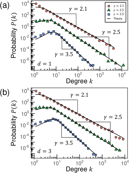
Figure 2: Degree distribution for RHGs with (a) $d=1$ and (b) $d=3$ at $\tau=0.5$ and $n=1000\cdot 2^{7}$. Each panel includes the degree distributions for (red) $\textsl{a}=1.1$ ($\gamma=2.1$), (green) $\textsl{a}=1.5$ ($\gamma=2.5$), and (blue) $\textsl{a}=2.5$ ($\gamma=3.5$). Degree distributions are binned logarithmically to suppress noise at large $k$ values. Solid lines are theoretical values for $P(k)$ prescribed by Eq. (34). For visibility, the probabilities corresponding to $\gamma=2.5$ and $\gamma=2.1$ are multiplied by $10^{2}$ and $10^{4}$, respectively. The scaling constant $\nu=10\times{dI_{d,1}\over 2^{d}}\left({\textsl{a}-1\over\textsl{a}}\right)^{2}{\sin(\pi\tau)\over\pi\tau}$, corresponding to $\langle k\rangle$ = 10 in the large $n$ limit.

The special case of $\textsl{a}=1$ ($\gamma=2$) is also well defined. In this case the expressions for $\langle k\rangle$ and $\langle k(\mathfrak{r})\rangle$ given by Eq. (26) remain valid but $\langle e^{-\mathfrak{r}}\rangle$ is now given by

$$\langle e^{-\mathfrak{r}}\rangle=\mathcal{R}e^{-\mathcal{R}}.$$ (35)

It is straightforward to verify that the scaling of $\mathcal{R}=\mathfrak{m}=\ln\left(n/\nu\right)$ in the $\textsl{a}=1$ case does not lead to the desired calibration of node degrees, $\langle k_{max}\rangle\sim n$ and $\langle k_{min}\rangle\sim 1$. Instead, the proper scaling is

$$\mathcal{R} = {\rm ln}\left(n/\nu\right),$$ (36)

$$\mathfrak{m} = \mathcal{R}-{\rm ln}\mathcal{R},$$ (37)

resulting in

$$\langle k\rangle_{n} = \nu{2^{d}\over dI_{d,1}}{\pi\tau\over\sin(\pi\tau)}{\rm ln}\left(n/\nu\right),$$ (38)

$$\langle k(\mathfrak{r})\rangle_{n} = {n\over\nu}\frac{\langle k\rangle}{{\rm ln}\left(n/\nu\right)}e^{-\mathfrak{r}}.$$ (39)

In other words, the $\textsl{a}=1$ ($\gamma=2$) case corresponds to graphs with $\langle k\rangle_{n}\sim\ln\left(n/\nu\right)$, as confirmed by Fig. 3. Degree distribution $P(k)$ matches a power-law with $\gamma=2$, as shown in Fig. 4. The resulting densification in the $\textsl{a}=1$ ($\gamma=2$) case is not specific to the RHG model but is a general property of all scale-free network models with $P(k)\sim k^{-2}$.

The divergence of $\langle k\rangle_{n}$ in the large $n$ limit does not impose problems for generating RHGs with desired $\langle k\rangle$ values. As we discuss in Section VI, in order to generate RHGs in the cold regime with $\gamma=2$ and desired $\langle k\rangle$ values, one needs to set $\textsl{a}=1$ and solve Eq. (38) for the corresponding $\nu$ values. The obtained $\nu$ values, in their turn, determine the sought values of radius $\mathcal{R}$ and chemical potential $\mathfrak{m}$, Eqs. (36) and (37).

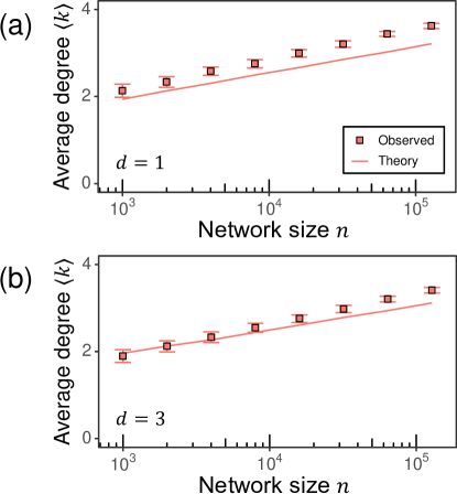
Figure 3: Expected degree $\langle k\rangle$ of RHGs with (a) $d=1$ and (b) $d=3$ in the case of $\textsl{a}=1$ at $\tau=0.5$. Each point is the average of $100$ simulations and the error bars display standard deviations. To avoid fluctuations associated with large degree nodes, we imposed a structural degree cutoff on generated RHGs, removing network nodes with degrees $k>n^{1/2}$. Solid lines are theoretical values for $\langle k\rangle$ prescribed by Eq. (38), corrected for the structural cutoff. The scaling constant is set to $\nu={dI_{d,1}\over 2^{d}}{\sin(\pi\tau)\over\pi\tau}$.

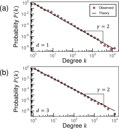
Figure 4: Degree distribution for RHGs with (a) $d=1$ and (b) $d=3$ in the case of $\textsl{a}=1$ at $\tau=0.5$ and $n=1000\cdot 2^{7}$. Degree distributions are binned logarithmically to suppress noise at large $k$ values. Solid lines are theoretical values for $P(k)$ based on a slope of $\gamma=2$. The scaling constant is set to $\nu={dI_{d,1}\over 2^{d}}{\sin(\pi\tau)\over\pi\tau}$.

IV.2 Critical regime, $\tau=1$

In the $\tau=1$ regime (23) and (19) can be approximated as:

$$\langle k\rangle_{n} ={(n-1)2^{d}\over dI_{d,1}}e^{\mathfrak{m}}$$ (40)

$$\times\left[d\ln\left({\pi\over 2}\right)\langle e^{-\mathfrak{r}}\rangle^{2}+2\langle e^{-\mathfrak{r}}\rangle\langle\mathfrak{r}e^{-\mathfrak{r}}\rangle-\mathfrak{m}\langle e^{-\mathfrak{r}}\rangle^{2}\right],$$

$$\langle k(\mathfrak{r})\rangle_{n} ={(n-1)2^{d}\over dI_{d,1}}e^{\mathfrak{m}-\mathfrak{r}}$$

$$\times\left[d\ln\left({\pi\over 2}\right)\langle e^{-\mathfrak{r}}\rangle+(\mathfrak{r}-\mathfrak{m})\langle e^{-\mathfrak{r}}\rangle+\langle\mathfrak{r}e^{-\mathfrak{r}}\rangle\right],$$

where $\langle\mathfrak{r}e^{-\mathfrak{r}}\rangle\equiv\int{\rm d}\mathfrak{r}\rho(\mathfrak{r})\mathfrak{r}e^{-\mathfrak{r}}$ is given by

$$\langle\mathfrak{r}e^{-\mathfrak{r}}\rangle=\left(\dfrac{\textsl{a}}{\textsl{a}-1}\right)\left[\left(\mathcal{R}-\dfrac{1}{\textsl{a}-1}\right)e^{-\mathcal{R}}+\dfrac{1}{\textsl{a}-1}e^{-\textsl{a}\mathcal{R}}\right].$$ (41)

Given that $\textsl{a}>1$, we drop the second terms in (27) and (41) to obtain:

$$\langle k(\mathfrak{r})\rangle_{n} ={(n-1)2^{d}\over dI_{d,1}}\left(\dfrac{\textsl{a}}{\textsl{a}-1}\right)$$ (42)

$$\times\left(d\log\left(\frac{\pi}{2}\right)-{1\over\textsl{a}-1}+\mathcal{R}-\mathfrak{m}+\mathfrak{r}\right)e^{\mathfrak{m}-\mathcal{R}-\mathfrak{r}}.$$

Similar to the $\tau<1$ regime, we demand $\langle k_{max}\rangle_{n}\sim n$ and $\langle k_{min}\rangle_{n}\sim 1$ to obtain the scaling relationships for $\mathfrak{m}$ and $\mathcal{R}$. For $\langle k_{max}\rangle_{n}=\langle k(0)\rangle_{n}$ and $\langle k_{min}\rangle_{n}=\langle k(\mathcal{R})\rangle_{n}$, we have

$$\langle k(0)\rangle_{n} \sim n\left(d\log\left(\frac{\pi}{2}\right)-{1\over\textsl{a}-1}+\mathcal{R}-\mathfrak{m}\right)e^{\mathfrak{m}-\mathcal{R}},$$ (43)

$$\langle k(\mathcal{R})\rangle_{n} \sim n\left(d\log\left(\frac{\pi}{2}\right)-{1\over\textsl{a}-1}+2\mathcal{R}-\mathfrak{m}\right)e^{\mathfrak{m}-2\mathcal{R}}.$$

Scaling $\langle k(0)\rangle_{n}\sim n$ and $\langle k(\mathcal{R})\rangle_{n}\sim 1$ is achieved when $\mathfrak{m}=\mathcal{R}$ and $\mathcal{R}e^{-\mathcal{R}}\sim{1\over n}$. Analogous to the cold regime, we set $\mathcal{R}^{-1}e^{\mathcal{R}}={n\over\nu}$, obtaining

$$\mathfrak{m}=\mathcal{R}=-W_{-1}\left(-\frac{\nu}{n}\right),$$ (44)

where $W_{-1}(\cdot)$ is the $W_{-1}$ branch of the Lambert $W$ function.

Using the scaling in (44), we obtain

$$\langle k\rangle_{n} =\dfrac{2^{d}}{dI_{d,1}}\left({\textsl{a}\over\textsl{a}-1}\right)^{2}$$ (45)

$$\times\left[1-\left(d\log\left(\frac{\pi}{2}\right)-\dfrac{2}{\textsl{a}-1}\right)\left(W_{-1}\left(-{\nu\over n}\right)\right)^{-1}\right]$$

$$\langle k(\mathfrak{r})\rangle_{n} =n{2^{d}\over dI_{d,1}}\left({\textsl{a}\over\textsl{a}-1}\right)\left(d\log\left(\frac{\pi}{2}\right)-{1\over\textsl{a}-1}+\mathfrak{r}\right)e^{-\mathfrak{r}}.$$

Hence, the critical regime corresponds to sparse graphs in the large $n$ limit, as confirmed by simulations in Fig. 5. Note that the convergence to the $n\rightarrow\infty$ asymptote of $\langle k\rangle=10$ is slower than in the cold regime, likely due to relatively large subleading terms in (45).

Degree distributions of RHGs in the critical regime seem to follow a power-law with the same exponent as in the cold regime:

$$P(k) \sim k^{-\gamma},$$ (46)

$$\gamma =\textsl{a}+1,$$

see Fig. 6. This is the case since the tail of $P(k)$ is dominated by nodes at small $\mathfrak{r}$ values. In the critical regime, $\langle k(\mathfrak{r})\rangle_{n}\sim e^{-\mathfrak{r}}$ for $\mathfrak{r}$ values close to $0$, similar to the cold regime, resulting in the same degree distribution exponent $\gamma$.

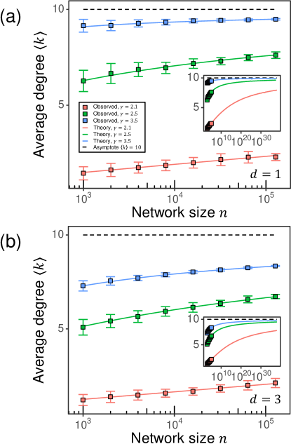
Figure 5: Expected degree $\langle k\rangle$ as a function of network size $n$ for RHGs in the critical ($\tau=1$) regime with (a) $d=1$ and (b) $d=3$. Each panel includes the results for (red) $\textsl{a}=1.1$ ($\gamma=2.1$), (green) $\textsl{a}=1.5$ ($\gamma=2.5$), and (blue) $\textsl{a}=2.5$ ($\gamma=3.5$). Each point is the average of $100$ simulations and the error bars display standard deviations. Solid lines are theoretical values for $\langle k\rangle$ prescribed by Eqs. (17) and (19) and the dashed line is the $n\to\infty$ limit of Eq. (45). The insets in (a) and (b) correspond to extended domains of $n$ values. Note that in the critical regime all 3 cases converge to the asymptotic value at a much slower rate than in the cold regime, while the $\textsl{a}=1.1$ case has not yet converged even within the extended domain of $n$ values.

Figure 6: Degree distribution for RHGs with (a) $d=1$ and (b) $d=3$ at $\tau=1$ and $n=1000\cdot 2^{7}$. Each panel includes the degree distributions for (red) $\textsl{a}=1.1$ ($\gamma=2.1$), (green) $\textsl{a}=1.5$ ($\gamma=2.5$), and (blue) $\textsl{a}=2.5$ ($\gamma=3.5$). Degree distributions are binned logarithmically to suppress noise at large $k$ values. For visibility, the probabilities corresponding to $\gamma=2.5$ and $\gamma=2.1$ are multiplied by $10^{2}$ and $10^{4}$, respectively. Solid lines are theoretical values for $P(k)$ prescribed by Eq. (34). The scaling constant $\nu$ is chosen such that $\nu=10\times{dI_{d,1}\over 2^{d}}\left({\textsl{a}-1\over\textsl{a}}\right)^{2}$, corresponding to $\langle k\rangle$ = 10 in the large $n$ limit.

To investigate the $\textsl{a}=1$ ($\gamma=2$) case of the critical regime, we need to re-examine the scaling of $\langle k(\mathfrak{r}=0)_{n}\rangle$ and $\langle k(\mathfrak{r}=\mathcal{R})_{n}\rangle$. To do so, we use Eq. (17) with $\tau=1$ and $\textsl{a}=1$, arriving, to the leading order, at

$$\langle k(\mathfrak{r}=\mathcal{R})\rangle = \frac{2^{d}\left(\frac{\pi}{2}\right)^{d}}{I_{d,1}}n,$$ (47)

$$\langle k(\mathfrak{r}=0)\rangle = \frac{3\times 2^{d-1}\left(\frac{\pi}{2}\right)^{d}}{I_{d,1}}n\mathcal{R}^{2}e^{\mathfrak{m}-2\mathcal{R}}.$$ (48)

It is seen from Eqs. (47) and (48) that the desired scalings of $\langle k_{max}\rangle_{n}=\langle k(\mathfrak{r}=0)\rangle_{n}\sim n$ and $\langle k_{min}\rangle_{n}=\langle k(\mathfrak{r}=\mathcal{R})\rangle_{n}~{}\sim 1$ are obtained if we set $R=\ln\left(n/\nu\right)$, and $\mathfrak{m}=R-2\ln R$. Then,

$$\langle k(\mathfrak{r})\rangle_{n} ={2^{d}\over dI_{d,1}}\frac{n}{\left[\ln\left(n/\nu\right)\right]^{2}}e^{-\mathfrak{r}}$$ (49)

$$\quad\times\left[{\rm Li}_{2}\left[-\left[\ln\left(\frac{n}{\nu}\right)\right]^{2}\left(\frac{\pi}{2}\right)^{d}e^{\mathfrak{r}-\mathcal{R}}\right]\right.$$

$$\qquad\qquad\left.-\,{\rm Li}_{2}\left[-\left[\ln\left(\frac{n}{\nu}\right)\right]^{2}\left(\frac{\pi}{2}\right)^{d}e^{\mathfrak{r}}\right]\right],$$

$$\langle k\rangle_{n} =\nu{2^{d}\over dI_{d,1}}\frac{1}{\left[\ln\left(n/\nu\right)\right]^{2}}$$

$$\quad\times\left[2{\rm Li}_{3}\left[-\left[\ln\left(\frac{n}{\nu}\right)\right]^{2}\left(\frac{\pi}{2}\right)^{d}\right]\right.$$

$$\qquad\qquad-{\rm Li}_{3}\left[-\left[\ln\left(\frac{n}{\nu}\right)\right]^{2}\left(\frac{\pi}{2}\right)^{d}e^{-\mathcal{R}}\right]$$

$$\qquad\qquad\left.-\,{\rm Li}_{3}\left[-\left[\ln\left(\frac{n}{\nu}\right)\right]^{2}\left(\frac{\pi}{2}\right)^{d}e^{\mathcal{R}}\right]\right],$$

and

$$\langle k\rangle_{n}\sim\nu\frac{2^{d}}{dI_{d,1}}\ln\left(\frac{n}{\nu}\right),$$ (50)

where ${\rm Li}_{s}(x)$ is the $s$-th order polylogarithm function. Like in the cold regime, the $\textsl{a}=1$ case in the critical regime corresponds to graphs with $\langle k\rangle_{n}\sim\ln\left(n/\nu\right)$, as confirmed by Fig. 7. The degree distribution for $\textsl{a}=1$ in the critical regime is shown in Fig. 8.

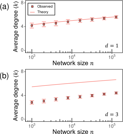
Figure 7: Expected degree $\langle k\rangle$ as a function of network size $n$ for RHGs with (a) $d=1$ and (b) $d=3$ for the case of $\textsl{a}=1$ at $\tau=1$. Each point is the average of $100$ simulations and the error bars display standard deviations. Solid lines are theoretical values for $\langle k\rangle$ prescribed by Eq. (49). The scaling constant is set to $\nu={dI_{d,1}\over 2^{d}}$.

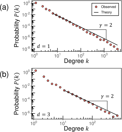
Figure 8: Degree distribution for RHGs with (a) $d=1$ and (b) $d=3$ in the case of $\textsl{a}=1$ at $\tau=1$ and $n=1000\cdot 2^{7}$. Degree distributions are binned logarithmically to suppress noise at large $k$ values. Solid lines are theoretical values for $P(k)$ based on a slope of $\gamma=2$. The scaling constant is set to $\nu={dI_{d,1}\over 2^{d}}$.

IV.3 Hot regime, $\tau>1$

In the $\tau>1$ case the Eqs. (17) and (19) can be approximated as

$$\langle k\rangle_{n} = (n-1)\,\mathcal{I}(d,\tau)\,e^{\mathfrak{m}/\tau}\langle e^{-\mathfrak{r}/\tau}\rangle^{2},$$ (51)

$$\langle k(\mathfrak{r})\rangle_{n} = {\langle k\rangle\over\langle e^{-\mathfrak{r}/\tau}\rangle}e^{-\mathfrak{r}/\tau},$$ (52)

where

$$\mathcal{I}(d,\tau)\equiv{\frac{1}{I_{d,1}}\int_{0}^{\pi}\frac{{\rm sin}^{d-1}\theta{\rm d}\theta}{{\rm sin}\left(\frac{\theta}{2}\right)^{d/\tau}}},$$ (53)

and

$$\langle e^{-\mathfrak{r}/\tau}\rangle\equiv\int_{0}^{\mathcal{R}}\rho(\mathfrak{r})e^{-{\mathfrak{r}/\tau}}{\rm d}\mathfrak{r}\approx{\textsl{a}\tau\over\textsl{a}\tau-1}\left(e^{-\mathcal{R}/\tau}-e^{-\textsl{a}/\mathcal{R}}\right).$$ (54)

Note that the expression for $\langle e^{-\mathfrak{r}/\tau}\rangle$ given by Eq. (54) is valid for all values of a and $\tau$ since $\textsl{a}\tau>1$.

Similar to the $\tau<1$ regime, we demand $\langle k_{max}\rangle_{n}\sim n$ and $\langle k_{min}\rangle_{n}\sim 1$ to obtain the scaling relationships for $\mathfrak{m}$ and $\mathcal{R}$:

$$\mathfrak{m}=\mathcal{R}=\tau\ln\left(n/\nu\right).$$ (55)

This scaling in combination with Eq. (51) leads in the large $n$ limit to

$$\langle k\rangle_{n}= \,\nu\,\mathcal{I}(d,\tau)\left(\textsl{a}\tau\over\textsl{a}\tau-1\right)^{2},$$ (56)

$$\langle k(\mathfrak{r})\rangle_{n}= {n\over\nu}\left(\textsl{a}\tau-1\over\textsl{a}\tau\right)\langle k\rangle e^{-\mathfrak{r}/\tau},$$

$$P(k)= \textsl{a}\tau\left[\langle k(\mathcal{R})\rangle\right]^{\textsl{a}\tau}\frac{\Gamma[k-\textsl{a}\tau]}{\Gamma[k+1]}\sim k^{-\gamma},$$

where $\gamma=\textsl{a}\tau+1$, confirmed by Fig. 9. Similar to the cold and critical regimes, RHGs in the hot regime are sparse and scale-free. Different from the cold and critical regimes, degree distribution exponent $\gamma$ in the hot regime depends on both a and $\tau$, as confirmed by Fig. 10.

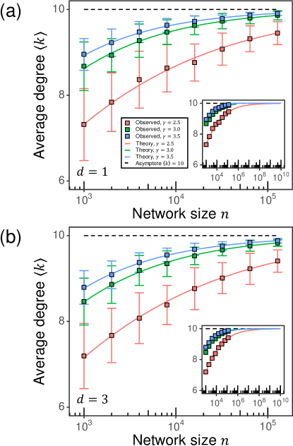
Figure 9: Expected degree $\langle k\rangle$ as a function of network size $n$ for RHGs in the hot ($\tau=1.5$) regime with (a) $d=1$ and (b) $d=3$. Each panel includes the results for (red) $\textsl{a}=1$ ($\gamma=2.5$), (green) $\textsl{a}=\frac{4}{3}$ ($\gamma=3.0$), and (blue) $\textsl{a}=\frac{5}{3}$ ($\gamma=3.5$). Each point is the average of $100$ simulations and the error bars display standard deviations. Solid lines are theoretical values for $\langle k\rangle$ prescribed by Eqs. (17) and (19) and the dashed line is the $n\to\infty$ limit for $\langle k\rangle$ given by Eq. (56). The insets in (a) and (b) correspond to extended domains of $n$ values.

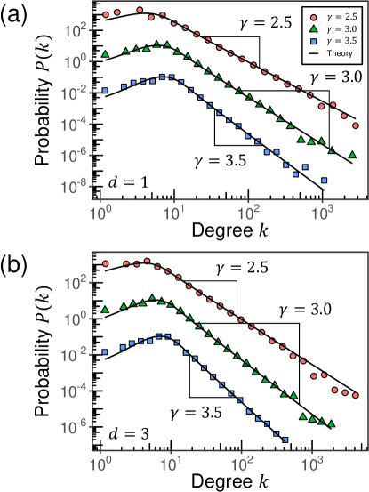
Figure 10: Degree distribution for RHGs with (a) $d=1$ and (b) $d=3$ at $\tau=1.5$ and $n=1000\cdot 2^{7}$. Each panel includes the degree distributions for (red) $\textsl{a}=1$ ($\gamma=2.5$), (green) $\textsl{a}=\frac{4}{3}$ ($\gamma=3.0$), and (blue) $\textsl{a}=\frac{5}{3}$ ($\gamma=3.5$). Degree distributions are binned logarithmically to suppress noise at large $k$ values. Solid lines are theoretical values for $P(k)$ prescribed by Eq. (56). For visibility, the probabilities corresponding to $\gamma=3.0$ and $\gamma=2.5$ are multiplied by $10^{2}$ and $10^{4}$, respectively. The scaling constant $\nu$ is chosen such that $\nu=10\times{1\over\mathcal{I}(d,\tau)}\left({\textsl{a}\tau-1\over\textsl{a}\tau}\right)^{2}$, corresponding to $\langle k\rangle~{}=~{}10$ in the large $n$ limit.

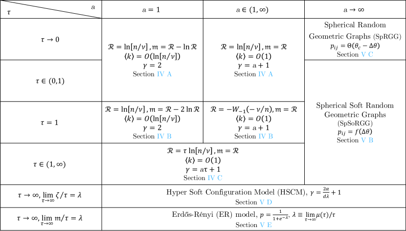
Figure 11: RHG regimes in terms of rescaled variables.

V Limiting cases of the RHG model

In this section, we analyze several important parameter limits of the RHG and show that they correspond to well-known graph ensembles.

V.1 $\tau\to 0$ limit in the cold regime

The case of $\tau=0$ is well-defined as the $\tau\to 0$ limit of the cold regime. The $T\to 0$ limit of the connection probability function in Eq. (12) is the step function

$$p_{ij}=\Theta\left(\mu-d_{ij}\right),$$ (57)

such that connections are established deterministically between node pairs separated by distances smaller than $\mu$.

In this case we have ${\pi\tau\over\sin\left(\pi\tau\right)}\to 1$ in (32), leading to

$$\langle k\rangle_{n} ={\nu 2^{d}\over dI_{d,1}}\left({\textsl{a}\over\textsl{a}-1}\right)^{2}$$ (58)

$$\times\left[1-2\left(\frac{n}{\nu}\right)^{1-\textsl{a}}+\left(\frac{n}{\nu}\right)^{2(1-\textsl{a})}\right],$$

$$\langle k(\mathfrak{r})\rangle_{n} ={n\over\nu}\left({\textsl{a}-1\over\textsl{a}}\right)\langle k\rangle e^{-\mathfrak{r}}\sum_{\ell=0}^{\infty}\left(\frac{\nu}{n}\right)^{\ell(\textsl{a}-1)}.$$

The resulting graphs are sparse and are characterized by ascale-free degree distribution $P(k)\sim k^{-\gamma}$, $\gamma=\textsl{a}+1$, similar to the $0<\tau<1$ case.

V.2 $\textsl{a}\to\infty$ limit: Spherical Soft Random Geometric Graphs (SpSoRGG)

In this limit the radial coordinate distribution (18) degenerates to

$$\rho(\mathfrak{r})\to\delta\left(\mathfrak{r}-\mathcal{R}\right).$$ (59)

As a result, all nodes are placed at the boundary of the hyperbolic ball $\mathbb{B}^{d+1}$ with $\mathfrak{r}_{i}=\mathcal{R}$. Even though the distances between nodes are still hyperbolic, they are fully determined by the angles on $\mathbb{S}^{d}$:

$$\zeta d_{ij}=\cosh^{-1}\left[\cosh\left(\frac{2\mathcal{R}}{d}\right)^{2}-\sinh\left(\frac{2\mathcal{R}}{d}\right)^{2}\sin\left(\Delta\theta_{ij}\right)\right].$$

Hence, connection probabilities $\{p_{ij}\}$ are fully determined by angles $\Delta\theta_{ij}$:

$$p_{ij}={1\over 1+\exp\left({\tilde{d}\left(\Delta\theta_{ij}\right)-\mathfrak{m}\over\tau}\right)},$$ (60)

where $\tilde{d}\left(\Delta\theta_{ij}\right)\equiv\frac{d\zeta}{2}d_{ij}$.

Effectively, in the $\textsl{a}\to\infty$ regime nodes are placed at the surface of the unit sphere $\mathbb{S}^{d}$ and connections are made with distance-dependent probabilities on the sphere. Hence, RHGs in the $\textsl{a}\to\infty$ limit are soft RGGs on $\mathbb{S}^{d}$.

V.3 $\textsl{a}\to\infty$, $\tau\to 0$ limit: Spherical Random Geometric Graphs (SpRGG)

If $\textsl{a}\to\infty$ and $\tau\to 0$ the connection probabilities in Eq. (16) become

$$p_{ij}=\Theta(\theta_{c}-\Delta\theta_{ij}),$$ (61)

where $\theta_{c}$ is the solution to the equation $\tilde{d}(\theta_{c})=\mathfrak{m}$. Thus, in this limit the RHG becomes the sharp random geometric graph on $\mathbb{S}^{d}$ (SpRGG).

The expected degree of the SpRGG equals the expected number of nodes that falls within an angle $\theta_{c}$ of the $\theta_{1}=0,...,\theta_{d}=0$ point,

$$\langle k\rangle=(n-1)\tilde{p},$$ (62)

where the volume of the $(d-1)$-dimensional sphere of radius $\theta_{c}$ in $\mathbb{S}^{d}$ is

$$\tilde{p}=\frac{\int_{0}^{\theta_{c}}\left[{\rm sin}\left(\theta\right)\right]^{d-1}{\rm d}\theta}{\int_{0}^{\pi}\left[{\rm sin}\left(\theta\right)\right]^{d-1}{\rm d}\theta}.$$ (63)

The degree distribution is thus binomial,

$$P(k)={\rm Bin}\left[n-1,\tilde{p}\right](k),$$ (64)

converging to the Poisson distribution with mean $\bar{k}$ if $\theta_{c}$ is such that $n\tilde{p}\to\bar{k}$. Since the Poisson distribution is the $\gamma\to\infty$ limit of the Pareto-mixed Poisson distribution (34), we refer to this regime as the $\gamma\to\infty$ case in Fig. 11.

V.4 $\zeta\to\infty$, $\tau\to\infty$ limit: Hyper Soft Configuration Model (HSCM)

In the $\zeta\to\infty$ limit, the hyperbolic distances in (7) degenerate to

$$d_{ij}=r_{i}+r_{j},$$ (65)

so that the angular coordinates of nodes are ignored in this limit. Further, if $\tau$ also tends to infinity, $\tau\rightarrow\infty$, but such that $\lim_{\zeta\to\infty}\frac{\zeta}{\tau}=\lambda>0$, where $\lambda$ is a constant, then the connection probability in Eq. (12) simplifies to

$$p_{ij}={1\over 1+e^{\omega_{i}}e^{\omega_{j}}},$$ (66)

which is the connection probability in the Hyper Soft Configuration Model (HSCM) van der Hoorn et al. (2018). Here, $\omega_{i}~{}=~{}\frac{d\lambda}{2}\left(r_{i}-\frac{\mu}{2}\right)$ are the Lagrange multipliers controlling expected node degrees. The Lagrange multipliers are drawn from the effective pdf

$$\rho(\omega) = \frac{2\alpha}{d\lambda}e^{\alpha\left(\frac{\mu}{2}-R\right)}e^{\frac{2\alpha}{d\lambda}\omega},$$ (67)

$$\omega \in \left(-\frac{d\lambda\mu}{4},\frac{d\lambda}{2}\left(R-\frac{\mu}{2}\right)\right).$$ (68)

The expected degrees in the HSCM are approximated by

$$\langle k(\omega_{i})\rangle =(n-1)\langle e^{-\omega}\rangle e^{-\omega_{i}},$$ (69)

$$\langle k\rangle =(n-1)\langle e^{-\omega}\rangle^{2},$$

where $\langle e^{-\omega}\rangle\equiv\int{\rm d}\omega\rho(\omega)e^{-\omega}$. By demanding that $\langle k\left(\omega(r=0)\right)\rangle_{n}\sim n$ and $\langle k\left(\omega(r=R)\right)\rangle_{n}\sim 1$ we obtain $R=\frac{2}{d\lambda}\ln(n)$, while $\mu=R$ in the case of $\frac{2\alpha}{d\lambda}>1$, and $\mu=\frac{2\alpha}{d\lambda}R$ in the case of $\frac{2\alpha}{d\lambda}<1$.

In both cases, $\langle k(\omega)\rangle\sim e^{-\omega}$ and graphs in the HSCM are sparse, while the conditional probability $P(k|\omega)$ is well-approximated by the Poisson distribution:

$$P(k|\omega)={1\over k!}e^{-\langle k(\omega)\rangle}\left[\langle k(\omega)\rangle\right]^{k},$$ (70)

see Ref. van der Hoorn et al. (2018). The resulting degree distribution $P(k)$ is a mixed Poisson distribution:

$$P(k)={1\over k!}\int_{-\frac{d\lambda\mu}{4}}^{\frac{d\lambda}{2}\left(R-\frac{\mu}{2}\right)}e^{-\langle k(\omega)\rangle}\left[\langle k(\omega)\rangle\right]^{k}\rho(\omega){\rm d}\omega,$$ (71)

with mixing parameter $\langle k(\omega)\rangle$. Using (21) and (22) we obtain

$$P(k) =\left(\gamma-1\right)\kappa_{0}^{\gamma-1}{\Gamma[k+1-\gamma,e^{\frac{d\lambda}{2}(R-\frac{\mu}{2})}\kappa_{0}]\over\Gamma[k+1]}$$ (72)

$$\sim k^{-\gamma},$$

where $\gamma={2\alpha\over d\lambda}+1$ and $\kappa_{0}\equiv e^{\frac{d\lambda}{2}\left(\frac{\mu}{2}-R\right)}{\langle k\rangle\over\langle e^{-\omega}\rangle}$.

Thus, the RHG model in the $\zeta\to\infty$, $\tau\to\infty$, $\zeta/\tau\to\lambda$ limit degenerates to the HSCM with a scale-free degree distribution with exponent $\gamma={2\alpha\over d\lambda}+1$.

V.5 $\tau\to\infty$ limit: the Erdős-Rényi (ER) model

The limit of $\tau\to\infty$ and finite $\zeta$ is the most degenerate case. Indeed, in this regime connection probabilities $p_{ij}$ become independent of hyperbolic distances $d_{ij}$ between the nodes:

$$p_{ij}=\lim_{\tau\to\infty}\frac{1}{1+e^{-\mu(\tau)/\tau}}.$$ (73)

It is seen from Eq. (73) that connection probabilities are non-trivial only in the case $\mu(\tau)\sim\tau$. In this case, connection probabilities are constant:

$$p_{ij}=p=\lim_{\tau\to\infty}\frac{1}{1+e^{-\lambda}},$$ (74)

where $\lambda\equiv\lim_{\tau\to\infty}\frac{\mu(\tau)}{\tau}$. By varying $\lambda\in(-\infty,\infty)$ one can tune connection probabilities $p\in(0,1)$ of the resulting ER graphs.

One can also check that the ER limit can be obtained either as the $\gamma\to\infty$ ($\alpha\to\infty$ or $\lambda\to 0$) limit of the HSCM, or as $\tau\to\infty$ limit of SpSoRGGs.

VI Random hyperbolic graphs: graph property perspective

From a graph property viewpoint, the RHG is instrumental in generating synthetic networks with desired properties. It follows from our analysis in Sections IV and V that depending on parameters $\left(n,\alpha,T,R\right)$, the RHG model can generate graphs with different expected degree and degree distribution. In particular, we observe in Section IV that RHGs in the cold, critical and hot regimes are characterized by scale-free degree distributions, $P(k)\sim k^{-\gamma}$, where exponent $\gamma\in[2,\infty)$ is a function of RHG temperature $\tau$ and node density parameter a. Radius $\mathcal{R}$ of the hyperbolic ball $\mathbb{B}^{d+1}$, on the other hand, controls the expected degree $\langle k\rangle$ and the sparsity of the resulting graphs.

Relying on these results, we can redefine the RHG model and its limiting cases in terms of parameters $\left(n,\gamma,\tau,\langle k\rangle\right)$. It is known that RHG temperature parameter $T$ controls the clustering coefficient of the resulting graph Krioukov et al. (2010). Yet the expressions for clustering in RHGs even in the $d=1$ case are quite complicated Candellero and Fountoulakis (2016); van der Kolk et al. (2021); Fountoulakis et al. (2021), and we do not attempt to obtain an analytical expression here for the clustering in the general case of $d>1$. Thus, we keep $\tau$ among the graph property parameters of the RHG model.

VI.1 RHG in the cold ($0\leq\tau<1$), critical ($\tau=1$), and hot ($1<\tau<\infty$) regimes

To generate an RHG in the cold regime with desired expected degree $\langle k\rangle$ and scale-free exponent $\gamma$, one sets the node density parameter a, chemical potential $\mathfrak{m}$, and the radius of $\mathbb{B}^{d+1}$ to

a $$= \gamma-1,$$ (75)

$$\mathfrak{m} = \mathcal{R}=\ln\left(n/\nu\right),$$ (76)

where $\nu$ is the solution of Eq. (32), which now takes the form of

$$\langle k\rangle =\nu{2^{d}\over dI_{d,1}}\left({\gamma-1\over\gamma-2}\right)^{2}{\pi\tau\over\sin(\pi\tau)}\times$$ (77)

$$\times\left[1-2\left(\frac{n}{\nu}\right)^{2-\gamma}+\left(\frac{n}{\nu}\right)^{2(2-\gamma)}\right],$$

where $I_{d,1}$ is given by (24).

When $\gamma=2$ in the cold regime, one must set

a $$= \gamma-1=1,$$ (78)

$$\mathcal{R} = \ln\left(n/\nu\right),$$ (79)

$$\mathfrak{m} = \mathcal{R}-{\rm ln}\mathcal{R},$$ (80)

and $\nu$ is obtained as the solution of Eq. (38), which takes the form of

$$\langle k\rangle=\nu{2^{d}\over dI_{d,1}}{\pi\tau\over\sin(\pi\tau)}{\rm ln}\left(n/\nu\right).$$ (81)

In the critical regime, one must set

a $$= \gamma-1,$$ (82)

$$\mathfrak{m} = \mathcal{R}=-W_{-1}\left(-{\nu\over n}\right),$$ (83)

where $\nu$ is determined by Eq. (45), which now takes the form of

$$\langle k\rangle =\dfrac{2^{d}}{dI_{d,1}}\left({\gamma-1\over\gamma-2}\right)^{2}$$ (84)

$$\times\left[1-\left(d\log\left(\frac{\pi}{2}\right)-\dfrac{2}{\gamma-2}\right)\left(W_{-1}\left(-{\nu\over n}\right)\right)^{-1}\right].$$

When $\gamma=2$ in the critical regime, one sets

$$\mathcal{R} = {\rm ln}\left(n/\nu\right),$$ (85)

$$\mathfrak{m} = \mathcal{R}-2{\rm ln}\mathcal{R},$$ (86)

while $\nu$ is obtained by solving the equation of $\langle k\rangle$ in Eq. (49), which now takes the form of

$$\langle k\rangle =\nu{2^{d}\over dI_{d,1}}\frac{1}{\left[\ln\left(n/\nu\right)\right]^{2}}$$ (87)

$$\quad\times\left[2{\rm Li}_{3}\left[-\left[\ln\left(\frac{n}{\nu}\right)\right]^{2}\left(\frac{\pi}{2}\right)^{d}\right]\right.$$

$$\qquad\qquad-{\rm Li}_{3}\left[-\left[\ln\left(\frac{n}{\nu}\right)\right]^{2}\left(\frac{\pi}{2}\right)^{d}\left({\nu\over n}\right)\right]$$

$$\qquad\qquad\left.-\,{\rm Li}_{3}\left[-\left[\ln\left(\frac{n}{\nu}\right)\right]^{2}\left(\frac{\pi}{2}\right)^{d}\left({n\over\nu}\right)\right]\right].$$

To generate an RHG in the hot regime, with given $\langle k\rangle$ and $\gamma$, one needs to set

a $$= \frac{\gamma-1}{\tau},$$ (88)

$$\mathfrak{m} = \mathcal{R}=\tau\ln\left(n/\nu\right),$$ (89)

where $\nu$ is given by

$$\langle k\rangle=\nu\,\mathcal{I}(d,\tau)\,\left(\gamma-1\over\gamma-2\right)^{2},\\$$ (90)

and $\mathcal{I}(d,\tau)$ is given by (53).

VI.2 Limiting cases of the RHG model: graph property perspective

Figure 12 summarizes properties of the RHG and its limiting cases in the $(\tau,\gamma)$ phase space. Within the $(\tau,\gamma)$ phase space, all the RHG temperature regimes condense into the heterogeneous ($2\leq\gamma<\infty$) soft-geometric ($0\leq\tau<\infty$) state.

The sharp-geometric limit ($\tau\to 0$) of this state is well-defined and is obtained by taking the $\tau\to 0$ limit in Eq. (77). In this case, to achieve RHGs with the desired expected degree $\langle k\rangle$ and a scale-free distribution exponent $\gamma>2$, one needs to set $\mathfrak{m}=\mathcal{R}=\ln(n/\nu)$, where $\nu$ is given by

$$\langle k\rangle=\nu{2^{d}\over dI_{d,1}}\left({\gamma-1\over\gamma-2}\right)^{2}\left[1-2\left(\frac{n}{\nu}\right)^{2-\gamma}+\left(\frac{n}{\nu}\right)^{2(2-\gamma)}\right].$$ (91)

By setting $\gamma\to\infty$ ($\textsl{a}\to\infty$) in the RHG, one arrives at Spherical Soft Random Geometric Graphs (SpSoRGG). Here nodes are placed at the boundary of the $\mathbb{B}^{d+1}$ ball, and connections are established with probabilities dependent on distances between the nodes on its $\mathbb{S}^{d}$ boundary, see Section V.2. Since SpSoRGGs are characterized by the Poisson degree distribution, we refer to them as the homogeneous ($\gamma\to\infty$) soft-geometric limit of the RHG. The expected degree of the SpSoRGG can be obtained by taking the $\gamma\to\infty$ limit of the RHG in the cold, critical, or hot regimes, depending of the $\tau$ value. In other words, to generate a SpSoRGG with prescribed $\tau$ and $\langle k\rangle$, one needs to set $\mathfrak{m}$, $\mathcal{R}$, and $\nu$ as follows

$$0<\tau <1:\mathfrak{m}=\mathcal{R}=\ln\left(n/\nu\right),~{}\langle k\rangle={\nu 2^{d}\over dI_{d,1}}{\pi\tau\over\sin(\pi\tau)};$$ (92)

$$\tau =1:\mathfrak{m}=\mathcal{R}=-W_{-1}(\nu/n),~{}\langle k\rangle={\nu 2^{d}\over dI_{d,1}};$$

$$\tau >1:\mathfrak{m}=\mathcal{R}=\tau\ln\left(n/\nu\right),~{}\langle k\rangle=\nu\,\mathcal{I}(d,\tau).$$

By taking the $\tau\to 0$ limit of the Spherical Soft RGG we arrive at the Spherical Sharp RGG, or simply Spherical Random Geometric Graph (SpRGG). Similar to its soft counterpart, nodes in the SpRGG are placed at the $\mathbb{B}^{d+1}$ boundary but connections are established deterministically between nodes separated by distances smaller then the threshold, Section V.2. Another possibility to arrive at the SpRGG is by taking the $\gamma\to\infty$ limit of the Sharp RHG. One can generate Spherical Sharp RGGs with desired expected degree $\langle k\rangle$ by setting $\mathfrak{m}=\mathcal{R}=\ln\left(n/\nu\right)$, and selecting $\nu$ from

$$\langle k\rangle={\nu 2^{d}\over dI_{d,1}}.$$ (93)

While both the Hyper Soft Configurational model (HSCM) and the Erdős-Rényi (ER) model are the $\tau\to\infty$ limits of the RHG, they belong to two distinct classes, as seen from the graph property perspective.

The HSCM model belongs to the non-geometric ($\tau\to\infty$) heterogeneous ($2\leq\gamma<\infty$) case and is a $\tau\to\infty$, $\zeta\to\infty$ limit of the RHG. To build RHGs with desired expected degree $\langle k\rangle$ and a scale-free degree distribution exponent $\gamma>2$, one sets $\mu=R=\frac{2}{d\lambda}\ln\left(\frac{n}{\nu}\right)$, where $\nu$ is the solution of

$$\langle k\rangle=\nu\left(\frac{\gamma-1}{\gamma-2}\right)^{2}\left[1-\left(\frac{\nu}{n}\right)^{\gamma-2}\right]^{2}.$$ (94)

The ER model, on the other hand, belongs to the non-geometric ($\tau\to\infty$) homogeneous ($\gamma\to\infty$) state and is a $\gamma\to\infty$ limit of the HSCM. Alternatively, the ER model can also be attained as the $\tau\to\infty$, $\zeta\to\infty$ limit of the SpSoRGG.

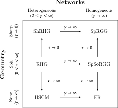
Figure 12: Limiting regimes of the RHG, graph property perspective.

VII Hyperbolic graph generator in $d+1$ dimensions

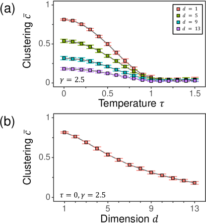
Figure 13: Average clustering coefficient $\bar{c}$ of nodes with degree $k>1$ (a) as a function of temperature $\tau$ for different dimensions $d$ and (b) as a function of dimension $d$ at $\tau=0$ for RHGs with $n=10^{4}$ and $\gamma=2.5$. Each point is the average of $100$ simulations and the error bars display standard deviations. The scaling constant $\nu$ is chosen such that $\langle k\rangle=10$ in the large $n$ limit.

We conclude by presenting a software package that generates RHGs of arbitrary dimensionality, to be specified by the user. The generator covers the cold ($\tau<1$), critical ($\tau=1$) and hot ($\tau>1$) regimes. The software package and detailed instructions on how to compile and use it are available at the Bitbucket repository Budel and Kitsak (2022).

The RHG generator can operate in two different modes: hybrid and model-based. In hybrid mode, the user provides expected degree $\langle k\rangle$, power-law exponent $\gamma$, rescaled temperature $\tau$ and dimension $d$. Eqs. (17) and (19) are solved for the rescaled radius $\mathcal{R}$ that yields the desired $\langle k\rangle$ using the bisection method. The triple integral that is found by combining Eqs. (17) and (19) is evaluated numerically using Monte Carlo integration with importance sampling through the GNU Scientific Library (GSL) Galassi et al. (2021). In model-based mode, the user directly provides the model parameters a, $\tau$, $\mathcal{R}$ (or $\nu$) and $d$. We expect the model-based mode to be instrumental for research purposes.

VIII Summary

In our work we have generalized the RHG to arbitrary dimensionality. In doing so, we have found the rescaling of network parameters, given by Eq. (15), that allows to reduce RHGs of arbitrary dimensionality to a single mathematical framework. Summarized in Fig. 11, our results indicate that RHGs exhibit similar connectivity properties, regardless of their dimensionality $d$. At the same time, we stress that higher dimensional realizations of the RHG model are expected to be different from the original $d=1$ RHG model with respect to other topological properties.

One such property is clustering. The properties of both average Candellero and Fountoulakis (2016) and degree-dependent Krioukov et al. (2010); Fountoulakis et al. (2021) clustering have been studied extensively in $d=1$ RHGs. It is well established that in $d=1$ there are two phases for RHGs with respect to the behavior of clustering. In the cold phase, $\tau<1$, RHGs are characterized by non-vanishing average Candellero and Fountoulakis (2016) and degree-dependent Krioukov et al. (2010); Fountoulakis et al. (2021) clustering. In the hot phase, $\tau>1$, clustering becomes size-dependent and vanishes in the large-$n$ limit. The critical temperature of $\tau=1$ corresponds to a continuous phase transition, which has been shown to be topological in nature, characterized by diverging entropy and atypical finite size scaling behavior of clustering van der Kolk et al. (2021). While we do not attempt to obtain analytical expressions for clustering here, we note that the degree-dependent clustering does depend on both dimensionality and temperature, see Fig. 13. This observation is in line with another work proposing to use the density of cycles to estimate network dimensionality Almagro et al. (2021). Yet it remains an open question what exactly is different between two RHGs of different dimensionalities whose clustering is matched by selecting appropriate temperatures.

Higher-dimensional RHGs may be instrumental in graph embedding tasks. Indeed, dimensionality of the latent space has been shown to impact the accuracy of many network inference tasks, including link prediction, clustering, and node classification Gu et al. (2021). One of the standard mapping approaches is Maximum Likelihood Estimation (MLE), finding node coordinates of the network of interest by maximizing the likelihood that the network was generated as an RHG in the latent space. The likelihood function in the case of $\mathbb{H}^{2}$ has been shown to be extremely non-convex with respect to node coordinates Papadopoulos et al. (2015a), making standard learning tools, like stochastic gradient descent, inefficient. Raising the dimensionality of the latent space $\mathbb{H}^{d+1}$ may lift some of the local maxima of the likelihood function, potentially leading to faster and more accurate graph embedding algorithms.

IX Acknowledgements

We thank F. Papadopoulos, M. Á. Serrano, M. Boguña, P. van der Hoorn, and T. van der Zwan for useful discussions and suggestions. This work was supported by ARO Grant No. W911NF-17-1-0491 and NSF Grant No. IIS-1741355. G. Budel and M. Kitsak were additionally supported by the NExTWORKx project, a collaboration between TU Delft and KPN on future telecommunication networks.

References

- Krioukov et al. (2009) D. Krioukov, F. Papadopoulos, A. Vahdat, and M. Boguñá, Curvature and Temperature of Complex Networks, Phys. Rev. E 80, 35101 (2009).
- Krioukov et al. (2010) D. Krioukov, F. Papadopoulos, M. Kitsak, A. Vahdat, and M. Boguñá, Hyperbolic Geometry of Complex Networks, Phys. Rev. E 82, 036106 (2010).
- McFarland and Brown (1973) D. D. McFarland and D. J. Brown, Social distance as a metric: A systematic introduction to smallest space analysis, in Bonds of Pluralism: The Form and Substance of Urban Social Networks (John Wiley, New York, 1973) pp. 213–252.
- Hoff et al. (2002) P. D. Hoff, A. E. Raftery, and M. S. Handcock, Latent Space Approaches to Social Network Analysis, J. Am. Stat. Assoc. 97, 1090 (2002).
- Serrano et al. (2008) M. Á. Serrano, D. Krioukov, and M. Boguñá, Self-Similarity of Complex Networks and Hidden Metric Spaces, Phys. Rev. Lett. 100, 078701 (2008).
- Papadopoulos et al. (2012) F. Papadopoulos, M. Kitsak, M. Á. Serrano, M. Boguñá, and D. Krioukov, Popularity versus Similarity in Growing Networks, Nature 489, 537 (2012).
- Zuev et al. (2015) K. Zuev, M. Boguñá, G. Bianconi, and D. Krioukov, Emergence of Soft Communities from Geometric Preferential Attachment, Sci. Rep. 5, 9421 (2015).
- Zheng et al. (2021) M. Zheng, G. García-Pérez, M. Boguñá, and M. Á. Serrano, Scaling up real networks by geometric branching growth, Proc Natl Acad Sci 118 (2021).
- Boguñá et al. (2010) M. Boguñá, F. Papadopoulos, and D. Krioukov, Sustaining the Internet with Hyperbolic Mapping. Nat. Commun. 1, 62 (2010).
- Kitsak et al. (2020) M. Kitsak, I. Voitalov, and D. Krioukov, Link Prediction with Hyperbolic Geometry, Phys. Rev. Res. 2, 043113 (2020).
- García-Pérez et al. (2019) G. García-Pérez, A. Allard, M. Á. Serrano, and M. Boguñá, Mercator: uncovering faithful hyperbolic embeddings of complex networks, New J. Phys. 21, 123033 (2019).
- Boguñá et al. (2008) M. Boguñá, D. Krioukov, and K. C. Claffy, Navigability of complex networks, Nat. Phys. 5, 74 (2008).
- Gulyás et al. (2015) A. Gulyás, J. J. Bíró, A. Kőrösi, G. Rétvári, and D. Krioukov, Navigable networks as Nash equilibria of navigation games, Nat. Commun. 6, 7651 (2015).
- Voitalov et al. (2017) I. Voitalov, R. Aldecoa, L. Wang, and D. Krioukov, Geohyperbolic Routing and Addressing Schemes, ACM SIGCOMM Comput. Commun. Rev. 47, 11 (2017).
- Ortiz et al. (2017) E. Ortiz, M. Starnini, and M. Á. Serrano, Navigability of temporal networks in hyperbolic space, Sci. Rep. 7, 15054 (2017).
- García-Pérez et al. (2018) G. García-Pérez, M. Boguñá, and M. Á. Serrano, Multiscale Unfolding of Real Networks by Geometric Renormalization, Nat. Phys. 14, 583 (2018).
- Muscoloni and Cannistraci (2019) A. Muscoloni and C. V. Cannistraci, Navigability evaluation of complex networks by greedy routing efficiency, Proc. Natl. Acad. Sci. 116, 1468 (2019).
- Serrano et al. (2012) M. Á. Serrano, M. Boguñá, and F. Sagués, Uncovering the Hidden Geometry Behind Metabolic Networks, Mol. Biosyst. 8, 843 (2012).
- Papadopoulos et al. (2015a) F. Papadopoulos, C. Psomas, and D. Krioukov, Network Mapping by Replaying Hyperbolic Growth, IEEE/ACM Trans. Netw. 23, 198 (2015a).
- Papadopoulos et al. (2015b) F. Papadopoulos, R. Aldecoa, and D. Krioukov, Network Geometry Inference Using Common Neighbors, Phys. Rev. E 92, 022807 (2015b).
- Muscoloni et al. (2017) A. Muscoloni, J. M. Thomas, S. Ciucci, G. Bianconi, and C. V. Cannistraci, Machine learning meets complex networks via coalescent embedding in the hyperbolic space, Nat. Commun. 8, 1615 (2017).
- Muscoloni and Cannistraci (2018a) A. Muscoloni and C. V. Cannistraci, Leveraging the nonuniform PSO network model as a benchmark for performance evaluation in community detection and link prediction, New J. Phys. 20 (2018a).
- Muscoloni and Cannistraci (2018b) A. Muscoloni and C. V. Cannistraci, Minimum curvilinear automata with similarity attachment for network embedding and link prediction in the hyperbolic space, (2018b), arXiv:1802.01183 .
- García-Pérez et al. (2020) G. García-Pérez, R. Aliakbarisani, A. Ghasemi, and M. Á. Serrano, Precision as a measure of predictability of missing links in real networks, Phys. Rev. E 101, 052318 (2020).
- Nickel and Kiela (2017) M. Nickel and D. Kiela, Poincare Embeddings for Learning Hierarchical Representations, Adv. Neural Inf. Process. Syst. (2017), arXiv:1705.08039 .
- Nickel and Kiela (2018) M. Nickel and D. Kiela, in 35th Int. Conf. Mach. Learn. ICML 2018 (2018) arXiv:1806.03417 .
- Dhingra et al. (2018) B. Dhingra, C. Shallue, M. Norouzi, A. Dai, and G. Dahl, in Proc. Twelfth Work. Graph-Based Methods Nat. Lang. Process. (Stroudsburg, PA, USA, 2018) pp. 59–69.
- Tifrea et al. (2019) A. Tifrea, G. Bécigneul, and O.-E. Ganea, in 7th Int Conf Learn Represent ICLR 2019, New Orleans, LA, USA, May 6-9, 2019 (OpenReview.net, 2019).
- Boguñá et al. (2021) M. Boguñá, I. Bonamassa, M. De Domenico, S. Havlin, D. Krioukov, and M. Á. Serrano, Network Geometry, Nat. Rev. Phys. 3, 114 (2021).
- Aldecoa et al. (2015) R. Aldecoa, C. Orsini, and D. Krioukov, Hyperbolic Graph Generator, Comput. Phys. Commun. 196, 492 (2015).
- Bringmann et al. (2019) K. Bringmann, R. Keusch, and J. Lengler, Geometric inhomogeneous random graphs, Theor Comput Sci 760, 35 (2019).
- Boguñá et al. (2020) M. Boguñá, D. Krioukov, P. Almagro, and M. Á. Serrano, Small worlds and clustering in spatial networks, Phys. Rev. Res. 2, 023040 (2020).
- Yang and Rideout (2020) W. Yang and D. Rideout, High Dimensional Hyperbolic Geometry of Complex Networks, Mathematics 8, 1861 (2020).
- Kovács et al. (2022) B. Kovács, S. G. Balogh, and G. Palla, Generalised popularity-similarity optimisation model for growing hyperbolic networks beyond two dimensions, Sci. Rep. 12, 968 (2022).
- Boguñá and Pastor-Satorras (2003) M. Boguñá and R. Pastor-Satorras, Class of Correlated Random Networks with Hidden Variables, Phys. Rev. E 68, 036112 (2003).
- Voitalov et al. (2019) I. Voitalov, P. van der Hoorn, R. van der Hofstad, and D. Krioukov, Scale-free networks well done, Phys. Rev. Res. 1, 033034 (2019).
- van der Hoorn et al. (2018) P. van der Hoorn, G. Lippner, and D. Krioukov, Sparse Maximum-Entropy Random Graphs with a Given Power-Law Degree Distribution, J. Stat. Phys. 173, 806 (2018).
- Candellero and Fountoulakis (2016) E. Candellero and N. Fountoulakis, Clustering and the Hyperbolic Geometry of Complex Networks, Internet Math. 12, 2 (2016), arXiv:1309.0459 .
- van der Kolk et al. (2021) J. van der Kolk, M. Á. Serrano, and M. Boguñá, A geometry-induced topological phase transition in random graphs, (2021), arXiv:2106.08030 .
- Fountoulakis et al. (2021) N. Fountoulakis, P. van der Hoorn, T. Müller, and M. Schepers, Clustering in a hyperbolic model of complex networks, Electron. J. Probab. 26 (2021).
- Budel and Kitsak (2022) G. Budel and M. Kitsak, The RHG Generator, https://bitbucket.org/gbudel/rhg-generator/ (2022).
- Galassi et al. (2021) M. Galassi et al., GNU Scientific Library Reference Manual (3rd Ed.), (2021), iSBN: 0954612078.
- Almagro et al. (2021) P. Almagro, M. Boguñá, and M. Á. Serrano, Detecting the ultra low dimensionality of real networks, (2021), arXiv:2110.14507 .
- Gu et al. (2021) W. Gu, A. Tandon, Y.-Y. Ahn, and F. Radicchi, Principled approach to the selection of the embedding dimension of networks, Nat. Commun. 12, 3772 (2021).