Deep Reinforcement Learning for IoT Networks: Age of Information and Energy Cost Tradeoff

Abstract

In most Internet of Things (IoT) networks, edge nodes are commonly used as to relays to cache sensing data generated by IoT sensors as well as provide communication services for data consumers. However, a critical issue of IoT sensing is that data are usually transient, which necessitates temporal updates of caching content items while frequent cache updates could lead to considerable energy cost and challenge the lifetime of IoT sensors. To address this issue, we adopt the Age of Information (AoI) to quantify data freshness and propose an online cache update scheme to obtain an effective tradeoff between the average AoI and energy cost. Specifically, we first develop a characterization of transmission energy consumption at IoT sensors by incorporating a successful transmission condition. Then, we model cache updating as a Markov decision process to minimize average weighted cost with judicious definitions of state, action, and reward. Since user preference towards content items is usually unknown and often temporally evolving, we therefore develop a deep reinforcement learning (DRL) algorithm to enable intelligent cache updates. Through trial-and-error explorations, an effective caching policy can be learned without requiring exact knowledge of content popularity. Simulation results demonstrate the superiority of the proposed framework.

I Introduction

In the foreseeable future, billions of electronic devices (e.g., smartphones, healthcare sensors, vehicles, smart cameras, smart home appliances, etc.), are anticipated to connect to the Internet, which constitutes the Internet of Things (IoT) [1, 2]. Massive numbers of IoT sensors will inevitably generate a tremendous amount of data, which could impose a heavy traffic burden and make wireless networks extremely congested. To cope with these challenges, pushing network resources from the cloud to the edge of wireless networks has been deemed as a promising approach for reducing traffic burden and enhancing user quality of service (QoS) in future IoT networks.

Considerable research attention has been devoted to caching policies to optimize communication performance metrics, e.g., transmission delay, traffic load, and power consumption [3, 4, 5]. However, these studies generally focus on caching multimedia content items that are usually in-transient once they are produced. In contrast, IoT sensing data cached in edge nodes are transient and could become outdated as time goes by. Hence, previous content caching strategies could not be readily utilized to provide fresh data in IoT services.

To capture data freshness of transient content items, the Age of Information (AoI) has emerged as an effective performance metric. AoI is defined by the time elapsed after the generation of IoT sensing data [6, 7]. It is desirable to minimize the average AoI of transient content items in the design of caching policies. On the other hand, frequent cache updates will cause considerable energy consumption at IoT sensors that usually have a rather limited battery capacity. To accommodate vast numbers of smart devices and extend the lifetime of IoT sensors, efficient cache update designs are needed to be developed towards fifth-generation (5G) and beyond communications.

Recently, machine learning, e.g., deep reinforcement learning (DRL), has been considered as a promising tool for resource management in IoT networks [2]. Some studies have utilized DRL to develop caching policies for IoT sensing. For instance, the study in [8] investigated a caching strategy design for the IoT by using federated DRL. However, it did not take into consideration data freshness. The authors in [9, 10] studied caching transient content items by minimizing the average AoI plus cache update cost. The cost of updating content in these studies was considered as the number of transmissions between sensors and edge nodes. This simple measurement was also used in [11] by assuming unit energy consumption per transmissions. A similar idea was also considered in [12]. Generally, the above-mentioned studies ignore the impact of time-varying content popularity.

This paper considers the scenario in which IoT sensors may produce the inhomogeneous size of transient content items that are required to be stored at the edge node via wireless links; meanwhile, the statistics of user requests towards IoT sensing data are uncertain and temporally evolving. We propose an intelligent policy to attain an equitable tradeoff between the average AoI and cache update cost, which is quantified as transmission energy consumption rather than the number of cache updates. The main contributions of this work are summarized as follows.

• We investigate the issue of how to preserve data freshness while reducing energy consumption at IoT sensors. Particularly, we consider cache updating given the inhomogeneous size of IoT sensing data, characteristics of wireless channels, and time-varying content popularity. To tackle the resulting decision-making in such a complex and dynamic environment, we propose a novel DRL-based framework.

• We develop a characterization of transmission energy consumption for uploading sensing data from IoT sensors to the edge node via wireless links. Particularly, we consider a realistic condition that wireless transmissions are effective when the received signal-to-noise ratio (SNR) is beyond a certain threshold.

• We conduct simulations to demonstrate that the proposed deep Q-network (DQN) algorithm can significantly reduce energy cost while slightly compromising average AoI. Under the scenario being studied, transmission energy consumption at IoT sensors witnesses a reduction of $52.7\%$, whereas average AoI is increased by 2.41 epochs compared with AoI-oriented results.

The remainder of this paper is organized as follows. Section II introduces the system model. Section III presents the MDP problem formulation, and Section IV develops a DRL-based algorithm. Section V presents simulation results, and Section VI concludes the paper.

II System Model

II-A System Operation

As illustrated in Fig. 1, we consider an IoT network, where the edge node (e.g., a small-cell base station) is deployed at the edge of wireless networks, which is connected to the cloud through fronthaul. There is a total of $F$ randomly distributed IoT sensors. Endowed with caching and computing units, the edge node is able to serve as a relay between data producers (e.g., IoT sensors) and data consumers (e.g., mobile users). More precisely, the edge node maintains a cache unit to aggregate sensing data produced by IoT sensors within its coverage; meanwhile, users can submit their requests to the edge node and retrieve desired content items for data analysis. We consider the scenario, where no direct links present between IoT sensors and users, similar to [13]. Let $\mathcal{F}=\{1,2,\cdots,F\}$ be the set of all indices of sensors. In addition, system operation time is assumed to be slotted into a sequence of epochs, i.e., $t=1,2,\cdots$. The sensing data cached at the edge node may be dynamically updated as time passed; but every content item, generated by a certain sensor, owns a specific content item index and generation epoch. As previously stated, we term IoT sensing data as transient content. For instance, content item $f$ with generation epoch $v_{f}^{t}$ means that, at epoch $t$, the caching content item available at the edge node is generated by sensor $f$ at epoch $v_{f}^{t}$; the associated generation epoch $v_{f}^{t}$ could be reset, once sensor $f$ is determined to upload a new measurement of content item $f$ into the edge node.

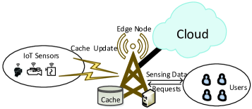
Figure 1: Illustration of an IoT network.

II-B Age of Information

We introduce a QoS metric, i.e., AoI, to capture how fresh a transient content item is. Particularly, the AoI of content item $f$ at epoch $t$, i.e., $o_{f}^{t}$, is defined as how many epochs have elapsed since this content item was generated. Accordingly, it gives rise to the following equation:

$$o_{f}^{t}=\max\{t-v_{f}^{t},1\},\forall f\in\mathcal{F},$$ (1)

which can take values from $\{1,2,\cdots,T_{\max}\}$; and $T_{\max}$ denotes the upper limit [14]. Let $N_{f}^{t}$ be the number of user requests for content item $f$ that are observed by the edge node at epoch $t$. Thus, the average AoI for satisfying user requests at epoch $t$ can be given as follows:

$$O^{t}=\frac{\sum_{f\in\mathcal{F}}o_{f}^{t}N_{f}^{t}}{\sum_{f\in\mathcal{F}}N_{f}^{t}}.$$ (2)

As caching content items gradually become outdated, a reasonable cache update is needed to serve user requests at the coming epochs. For ease of discussion, we assume that each IoT sensor is able to upload its sensing data to the edge node within a single epoch. That is, the AoI of a stale content turns to be 1 as long as the associated sensor is chosen to upload the current measurement of this content item. For instance, as depicted in Fig. 2, when a transient content is selected to update at epoch $t_{1}$, the corresponding AoI reduces to 1 at epoch $t_{1}+1$; otherwise, the AoI will increment by 1 after every epoch.

II-C Transmission Energy Consumption

To carry out cache updating, IoT sensors need access the edge node via wireless links; and orthogonal frequency bandwidths are allocated to different IoT sensors to avoid interference. Thus, the received SNR at the edge node concerning the $f$-th sensor can be given by:

$$\gamma_{f}=\frac{P_{f}\chi_{f}^{2}|\kappa_{f}|^{2}}{N_{0}B},\forall f\in\mathcal{F},$$ (3)

where $P_{f}$ denotes transmission power at the $f$-th sensor; coefficient $\chi_{f}$ denotes the impacts of the path loss and antenna gain; $\kappa_{f}$ denotes the small-scale fading component; $N_{0}$ is the power spectrum density; and $B$ denotes the channel bandwidth. We further assume that $|\kappa_{f}|$ follows the following Rayleigh distribution, i.e., $x\exp(-x^{2}/2)$. We consider transmissions between IoT sensors and the edge node are effective under the condition that the received SNR surpasses a pre-specified threshold $\gamma_{th}$. Given the storage size of sensing data from the $f$-th sensor as $s_{f}$ bits, we present the average transmission energy consumption in the following Proposition.

Proposition 1

The average transmission energy consumption $\bar{E}_{f}$ for the $f$-th IoT sensor ($\forall f\in\mathcal{F})$ to upload its sensing data is given by:

$$\bar{E}_{f}=\frac{\log(2)\times P_{f}s_{f}}{\log(2)\times r_{th}\exp\left(-\frac{\gamma_{th}}{2\beta_{f}}\right)+B\exp\left(\frac{1}{2\beta_{f}}\right)\mathcal{\rho}_{f}(\gamma_{th}+1)},$$ (4)

where function $\rho_{f}(\cdot)$ is defined as:

$$\rho_{f}(x)\triangleq\int_{x}^{+\infty}\frac{1}{x}\exp\bigg{(}-\frac{x}{2\beta_{f}}\bigg{)}dx,$$ (5)

and $\beta_{f}=P_{f}\chi_{f}^{2}/(N_{0}B)$; $r_{th}$ denotes the data rate threshold, given as follows:

$$r_{th}\triangleq\log_{2}(1+\gamma_{th}).$$ (6)

Proof.

Due to the page limit, we only sketch the basic idea here. Since the edge node would fail to decode information if the received SNR is lower than the required threshold $\gamma_{th}$, one can first compute the corresponding outage probability due to channel fading. The next step is to estimate the average transmission delay by calculating the expected transmission data rates. Finally, the average transmission energy consumption is given by the product of transmission power and average transmission delay. ∎

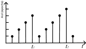
Figure 2: Illustration of the AoI of a specific transient content. Epochs of cache updates are denoted by $t_{1}$ and $t_{2}$.

Clearly, owing to limited battery levels at sensors and massive connections in IoT networks, it is crucial to find the best choice at each epoch to perform cache update so as to obtain an effective tradeoff between AoI and energy cost. Note that, the average AoI (e.g., see (2)) highly depends on content popularity distribution that usually exhibits temporal dynamics; meanwhile, energy consumption (e.g., see (4)) comes to storages of sensing data and channel statistics which are usually inhomogeneous among different sensors. Aware of this, we formulate an MDP based online cache update problem in the following section.

III MDP Problem Formulation

Typically, an MDP can be described by a tuple $(\mathcal{S},\mathcal{A},\mathcal{P},R,\gamma)$, where $\mathcal{S}$ denotes the state space containing all possible states $\boldsymbol{S}$; $\mathcal{A}$ denotes the action space collecting all possible actions $\boldsymbol{A}$; $\mathcal{P}$ collects transition probabilities $Pr\{\boldsymbol{S}^{\prime}|\boldsymbol{S},\boldsymbol{A}\}$; $R$ denotes a reward fed back to the agent after executing an action; and $\gamma\in[0,1)$ is a discount factor. In the online cache update problem, the edge node is anticipated to act as the agent; and we customize the above-mentioned elements in an MDP as follows.

• State: At each epoch, the edge node has exact knowledge of the AoI of caching content items as well as user requests. Hence, we define the system state as follows:

  $$\boldsymbol{S}^{t}=\left(\{o_{f}^{t}\}_{f\in\mathcal{F}},\{N_{f}^{t}\}_{f\in\mathcal{F}}\right).$$ (7)

• Action: Similar to study [11], let $\{0,1,\cdots,F\}$ be the action space. When action $\boldsymbol{A}^{t}=0$, it implies that no content is selected; otherwise, we push the new version of content item $\boldsymbol{A}^{t}\in\mathcal{F}$ into the cache unit. As such, it gives rise to the following relation:

  $$o_{f}^{t+1}=(o_{f}^{t}+1)\times\mathcal{I}(f,\boldsymbol{A}^{t})+\mathcal{I}(f,\boldsymbol{A}^{t}),\forall f\in\mathcal{F},$$ (8)

  where $\mathcal{I}(\cdot)$ is an indicator function. Clearly, cache update should be carried out after the occurrence of state $\boldsymbol{S}^{t}$, i.e., after user requests are revealed. Subsequently, the system is expected to transfer to a new state $\boldsymbol{S}^{t+1}$ with transition probability $Pr\{\boldsymbol{S}^{t+1}|\boldsymbol{S}^{t},\boldsymbol{A}^{t}\}$.

• Reward: The agent in an MDP is required to receive a reward signal $R^{t+1}$ along with the appearance of state $\boldsymbol{S}^{t+1}$. Recall that we aim to minimize the average AoI for satisfying user requests during the upcoming epoch while reducing transmission energy consumption. Hence, it is envisioned to minimize the following average weighted cost, i.e.:

  $$C^{t+1}=\frac{\sum_{f\in\mathcal{F}}o_{f}^{t+1}N_{f}^{t+1}}{\sum_{f\in\mathcal{F}}N_{f}^{t+1}}+\eta\bar{E}_{f}|_{f=\boldsymbol{A}^{t}},$$ (9)

  where the first term on the right-hand side denotes the average AoI at epoch $t+1$; and $\eta\geq 0$ is a constant to strike the balance between the average AoI and energy cost. We denote $\bar{E}_{0}=0$ for notational convenience. In accordance with the objective in (9), the reward signal of the proposed framework is designed as follows:

  $$R^{t+1}=-C^{t+1},$$ (10)

  which is supposed to be received at epoch $t+1$.

To this end, we need to find an optimal policy $\pi^{*}$ that maximizes the expected discounted cumulative reward, i.e.:

$$\pi^{*}=\arg\max_{\pi}\mathbb{E}[V^{t}|\pi],$$ (11)

where the expectation is over all possibilities of $\{\boldsymbol{S}^{t},\boldsymbol{A}^{t},\boldsymbol{S}^{t+1},R^{t+1}\}$, and the discounted cumulative reward is given by:

$$V^{t}=\sum_{\tau=0}^{\infty}(\gamma)^{\tau}R^{t+\tau+1}.$$ (12)

Since transition probability, i.e., $Pr\{\boldsymbol{S}^{\prime}|\boldsymbol{S},\boldsymbol{A}\}$, is generally difficult to acquire in practical applications, we move on to propose a DRL-based algorithm to address this problem through trial-and-error interactions with the environment.

IV Proposed DQN Based Algorithm

In this section, we propose an intelligent cache update design for an IoT network by adopting the state-of-art RL approaches, e.g., DQN. The key idea of this approach is built on utilizing deep neural networks (DNNs) to learn the Q-value function:

$$Q(\boldsymbol{S},\boldsymbol{A})=\mathbb{[}V^{t}|\boldsymbol{S}=\boldsymbol{S}^{t},\boldsymbol{A}=\boldsymbol{A}^{t},\pi^{*}],$$ (13)

which indicates the expected cumulative reward after executing action $\boldsymbol{A}^{t}$ and then following policy $\pi^{*}$; as such, an optimal action can be given by the one attaining the maximum Q-value under current state $\boldsymbol{S}^{t}$, i.e.:

$$\boldsymbol{A}^{*}=\arg\max_{\boldsymbol{A}}Q(\boldsymbol{S}^{t},\boldsymbol{A}).$$ (14)

According to the Bellman Optimality Equality in [15], we have the following recursive result:

$$Q(\boldsymbol{S}^{t},\boldsymbol{A}^{t})=R^{t+1}+\gamma\max_{\boldsymbol{A}^{\prime}\in\mathcal{A}}Q(\boldsymbol{S}^{t+1},\boldsymbol{A}^{\prime}).$$ (15)

In general, DQN entails maintaining two networks, i.e., Q-network and target Q-network [16]. Specifically, Q-network $Q_{\boldsymbol{\theta}}(\boldsymbol{S},\boldsymbol{A})$ can be constructed by a plain DNN, which is parametrized by $\boldsymbol{\theta}$. Readers are referred to [16] for greater detail. Target Q-network $Q_{\boldsymbol{\theta}^{-}}(\boldsymbol{S},\boldsymbol{A})$ is parametrized by $\boldsymbol{\theta}^{-}$, which is designed in the same manner as Q-network and can be used to calculate target values for network training.

The training procedure is introduced as follows. To aggregate training data, we leverage Replay Buffer (RB) to store historical experiences, e.g., $\xi^{t}=(\boldsymbol{S}^{t},\boldsymbol{A}^{t},\boldsymbol{S}^{t+1},R^{t+1})$. We assume that RB can store a total of $N$ experiences; and the stalest experience should be replaced by the fresh one as long as RB is fully filled. Subsequently, at each iteration, we randomly draw a mini-batch of experiences $\Xi_{N}$ from RB to update $\boldsymbol{\theta}$ by minimizing the following loss:

$$\hfill Loss=\mathbb{E}_{\xi^{t}\sim\Xi_{N}}\bigg{[}\big{(}y^{t}-Q_{\boldsymbol{\theta}}(\boldsymbol{S}^{t},\boldsymbol{A}^{t})\big{)}^{2}\bigg{]},$$ (16)

where $y^{t}$ denotes the target value, i.e.:

$$R^{t+1}+\gamma\max_{\boldsymbol{A}^{\prime}}Q_{\boldsymbol{\theta}^{-}}(\boldsymbol{S}^{t+1},\boldsymbol{A}^{\prime}).$$ (17)

Thus, adopting stochastic gradient descent approaches, parameter $\boldsymbol{\theta}$ can be updated as follows:

$$\boldsymbol{\theta}\leftarrow\boldsymbol{\theta}-\alpha\bigg{[}\big{(}Q_{\boldsymbol{\theta}}(\boldsymbol{S}^{t},\boldsymbol{A}^{t})-y^{t}\big{)}\nabla_{\boldsymbol{\theta}}Q_{\boldsymbol{\theta}}(\boldsymbol{S}^{t},\boldsymbol{A}^{t})\bigg{]},$$ (18)

where $\alpha$ is the learning rate. With regard to $\boldsymbol{\theta}^{-}$, it can be updated by $\boldsymbol{\theta}^{-}\leftarrow\boldsymbol{\theta}$ every $T_{0}$ iterations. Concerning exploration, we adopt the $\varepsilon$-greedy policy to generate actions: at each epoch, taking an action randomly drawn from $\{0,\cdots,F\}$ with probability $\varepsilon$ whereas taking an optimized action $\boldsymbol{A}^{*}=\arg\max_{\boldsymbol{A}}Q_{\boldsymbol{\theta}}(\boldsymbol{S},\boldsymbol{A})$ with probability $1-\varepsilon$. This is because the success of RL replies to visiting different state-action pairs so as to aggregate sufficient experiences to infer better actions and avoid suboptimal estimations of Q-value function. Finally, we summarize the proposed DRL-based cache update in Algorithm 1.

Algorithm 1 DRL-Based Cache Update for IoT Networks

Initialize $F$, $\boldsymbol{S}^{0}$, $\varepsilon$, $\gamma$, $\alpha$, $T_{0}$

Initialize parameter of Q-network $\boldsymbol{\theta}$,

Initialize parameter of target Q-network $\boldsymbol{\theta^{-}}$

Initialize RB

for $t=0,1,2,\cdots$ do

     Input $\boldsymbol{S}^{t}$ to Q-network and obtain $Q_{\boldsymbol{\theta}}(\boldsymbol{S}^{t},\boldsymbol{A}),\forall\boldsymbol{A}\in\mathcal{A}$

     Execute action $\boldsymbol{A}^{t}$ according to $\varepsilon$-greedy policy

     Observe $\boldsymbol{S}^{t+1}$, $R^{t+1}$

     Store $\left(\boldsymbol{S}^{t},\boldsymbol{A}^{t},\boldsymbol{S}^{t+1},R^{t+1}\right)$ into RB.

     if Remainder $(t,T_{0})==0$ then

         $I=1$

     else

         $I=0$

     end if

     TrainDQN($\gamma$, $\alpha$, $I$, RB, $\boldsymbol{\theta}$, $\boldsymbol{\theta^{-}}$)

end for

procedure TrainDQN($\gamma$, $\alpha$, $I$, RB, $\boldsymbol{\theta}$, $\boldsymbol{\theta^{-}}$)

     Randomly sample a batch experiences $\Xi_{N}$ from RB

     for each $\xi^{t}=\left({\boldsymbol{S}^{t},\boldsymbol{A}^{t},\boldsymbol{S}^{t+1},R^{t+1}}\right)\in\Xi_{N}$ do

         Calculate $y^{t}$ by (17)

     end for

     Calculate $Loss$ by (16)

     $\boldsymbol{\theta}\leftarrow\boldsymbol{\theta}-\alpha\nabla_{\boldsymbol{\theta}}Loss$

     if $I==1$ then

         Update the target Q-network by $\boldsymbol{\theta^{-}}\leftarrow\boldsymbol{\theta}$

     end if

end procedure

V Performance Evaluation

V-A Simulation Setup

In this section, we investigate the performance of the proposed algorithm. We consider the following IoT network: one edge node is deployed which covers a circle of radius 100 m; a total of 20 IoT sensors are randomly distributed within the coverage of the edge node; the storage size of each content item is randomly drawn from $[50,100]$ MB. Regarding communications between the edge node and sensors, the channel bandwidth is set as 10 MHz; large-scale fading is specified by the model used in [17]; noise spectrum density is -172 dBm; and transmission power of IoT sensors is 20 dBm. We consider there are at most 100 users requesting content by following Zipf distributions [17], i.e.:

$$p_{f}=\zeta_{f}^{-\kappa}/\sum_{f^{\prime}\in\mathcal{F}}\zeta_{f^{\prime}}^{-\kappa},$$ (19)

where rank orders of content items, e.g., $\{\zeta_{f}\}$, are randomly evolving according to a certain probability transmission matrix; and the skewness factor, e.g., $\kappa$, is randomly drawn from $\{0.5,1,1.5,2\}$. In the default setup, we consider that the average AoI and energy consumption are of equal importance, i.e., $\eta=1$.

To implement algorithm, the Q-network compromises three hidden layers with 512, 256, 128 neurons, respectively. The learning rate is set as 0.001. In $\varepsilon$-greedy policy, we take a random action with probability $\varepsilon=0.9$; then, $\varepsilon$ is decayed by 0.995 every iteration until 0.05. A mini-batch of 100 experiences is randomly sampled from the RB that has at most 5000 experiences. We update target Q-network every 100 epochs. The discount factor is 0.99. In addition, the following baselines are considered for algorithm comparisons:

• Most Popular Update (MPU): At every epoch, we consider to update the content item that receives the highest attention from users, i.e.:

  $$\boldsymbol{A}^{t}=\arg\max_{f\in\mathcal{F}}\frac{N_{f}^{t}}{\sum_{f^{\prime}\in\mathcal{F}}N_{f^{\prime}}^{t}}.$$ (20)

• Oracle Update (OU): We assume that the exact knowledge of up-coming user requests, e.g., $\{N_{f}^{t+1}\}$, is available at current epoch $t$. Then, we conduct cache update similar to the proposed DQN. This scheme simply serves as a baseline here and is not possible in reality.

• Random Update (RU): At every epoch, we randomly select an action from the action space, i.e., $\{0,1,\cdots,F\}$. This serves as a lower bound for the proposed algorithm.

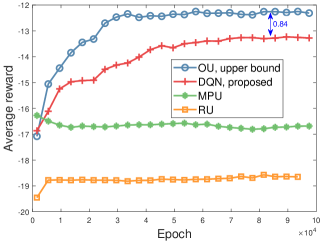
Figure 3: Convergence behavior of the proposed algorithm.

V-B Learning Curves

We first illustrate the learning curves of the proposed algorithm in Fig. 3. For illustrative purposes, we show the moving average results, which are attained by averaging rewards over $N=10000$ epochs, i.e., $\sum_{\tau=t-N+1}^{t}R^{\tau}/N$. Moreover, the resulting reward is less than zero since it is defined as the negative value of average weighted cost; see (10). It can be observed that, in the initial stage, the learning curve of the proposed algorithm increases rapidly and surpasses the curve of MPU; after 10000 epochs, it continuously increases; as more states are visited with time elapses, the resulting reward gradually grows larger, eventually converging to a higher level than that of MPU and RU. Note that, the average reward achieved by DQN is only 0.84 less than the upper bound, i.e., achieved by OU, whereas it exceeds the results of MPU and RU by 28.8% and 40.4%, respectively. This result implies that the proposed DQN algorithm is able to not only track the dynamics of user preferences towards content items but also adapt to energy costs among different sensors in physical-layer transmissions. These observations corroborate the remarkable performance of the proposed algorithm.

V-C Tradeoff Between AoI and Energy Cost

To investigate the tradeoff between AoI and energy cost, we vary factor $\eta$ and plot the results of average total cost, the average AoI, and average transmission energy in Figs. 4 - 6, respectively. As can be seen in Fig. 4, under different $\eta$, the proposed algorithm performs very close to the upper bound, and significantly outperforms other baselines, i.e., MPU and RU. For instance, when $\eta=20$, the achieved average weighted cost can be reduced by 54.9% and 44.3% in comparison to MPU and RU, respectively. These findings again demonstrate the advantages of the proposed DRL-based cache update and also validate its robustness toward factor $\eta$.

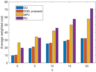
Figure 4: Average weighted cost.

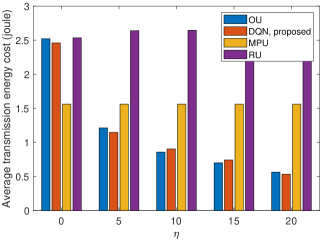
Figure 5: Average transmission energy cost.

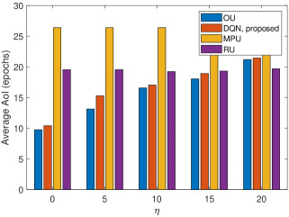
Figure 6: Average AoI.

Clearly, a larger $\eta$ implies that we pay more attention to minimizing energy consumption. As can be seen in Fig. 5, average energy costs, achieved by DQN and OU, drop off as $\eta$ becomes larger while other baselines only witness rather slight fluctuations without aware of AoI and energy cost tradeoff. On the other hand, in Fig. 6, we observe a reverse trend; that is, the caching content items become staler as $\eta$ grows larger. We conjecture that cache update could happen less frequently such that sensing data available at the cache unit becomes outdated. It is worth pointing out that when $\eta=5$, the achieved average AoI (by DQN) only degrades 2.41 while we can see a notable reduction of 52.7% in energy cost in contrast with the case $\eta=0$. If we continue increasing $\eta$, the reduction in energy consumption is quite limited yet at the cost of worsening AoI. Hence, it is necessary to choose a suitable $\eta$ to balance AoI and energy cost in real applications.

VI Conclusion

In this paper, we have put forth a deep reinforcement learning framework for online cache updating in IoT networks under dynamic content popularity. The objective of this framework is to minimize the weighted average AoI plus energy cost. We have developed a characterization of transmission energy consumption at IoT sensors. Through trial-and-error explorations, the proposed DQN algorithm is capable of adapting to temporal dynamics of user requests as well as the inhomogeneous content size and channel statistics among different IoT sensors. Simulation results have been presented to demonstrate the effectiveness of the proposed design and reveal how transmission energy consideration compromises data freshness.

References

- [1] S. Madakam, V. Lake, V. Lake, V. Lake et al., “Internet of things (IoT): A literature review,” Int. J. Comput. Commun., vol. 3, no. 05, p. 164, May 2015.
- [2] M. Chen, U. Challita, W. Saad, C. Yin, and M. Debbah, “Artificial neural networks-based machine learning for wireless networks: A tutorial,” IEEE Commun. Surveys Tuts., vol. 21, no. 4, pp. 3039–3071, Fourthquarter 2019.
- [3] X. Wu, Q. Li, X. Li, V. C. Leung, and P. Ching, “Joint long-term cache updating and short-term content delivery in cloud-based small cell networks,” IEEE Trans. Commun., vol. 68, no. 5, pp. 3173 – 3186, May 2020.
- [4] X. Wu, Q. Li, V. C. Leung, and P. Ching, “Joint fronthaul multicast and cooperative beamforming for cache-enabled cloud-based small cell networks: An MDS codes-aided approach,” IEEE Trans. Wireless Commun., vol. 18, no. 10, pp. 4970–4982, Oct. 2019.
- [5] X. Li, X. Wang, P.-J. Wan, Z. Han, and V. C. Leung, “Hierarchical edge caching in device-to-device aided mobile networks: Modeling, optimization, and design,” IEEE J. Sel. Areas Commun., vol. 36, no. 8, pp. 1768–1785, June 2018.
- [6] S. Kaul, R. Yates, and M. Gruteser, “Real-time status: How often should one update?” in Proc. IEEE INFOCOM, Mar. 2012, pp. 2731–2735.
- [7] Y. Sun, E. Uysal-Biyikoglu, R. D. Yates, C. E. Koksal, and N. B. Shroff, “Update or wait: How to keep your data fresh,” IEEE Trans. Inf. Theory, vol. 63, no. 11, pp. 7492–7508, Nov. 2017.
- [8] X. Wang, C. Wang, X. Li, V. C. Leung, and T. Taleb, “Federated deep reinforcement learning for internet of things with decentralized cooperative edge caching,” IEEE Internet Things J., to appear, 2020.
- [9] M. Ma and V. W. Wong, “A deep reinforcement learning approach for dynamic contents caching in HetNets,” arXiv preprint arXiv:2004.07911, 2020.
- [10] E. T. Ceran, D. Gündüz, and A. György, “A reinforcement learning approach to age of information in multi-user networks,” in Proc. IEEE PIMRC, Sept. 2018, pp. 1967–1971.
- [11] M. Hatami, M. Jahandideh, M. Leinonen, and M. Codreanu, “Age-aware status update control for energy harvesting IoT sensors via reinforcement learning,” arXiv preprint arXiv:2004.12684, 2020.
- [12] E. T. Ceran, D. Gündüz, and A. György, “Reinforcement learning to minimize age of information with an energy harvesting sensor with HARQ and sensing cost,” in Proc. IEEE INFOCOM Wkshps, Apr. 2019, pp. 656–661.
- [13] D. Niyato, D. I. Kim, P. Wang, and L. Song, “A novel caching mechanism for Internet of things (IoT) sensing service with energy harvesting,” in Proc. IEEE ICC, May 2016, pp. 1–6.
- [14] M. A. Abd-Elmagid, H. S. Dhillon, and N. Pappas, “A reinforcement learning framework for optimizing age-of-information in RF-powered communication systems,” IEEE Trans. Commun., vol. 68, no. 8, pp. 4747–4760, Aug., 2020.
- [15] R. S. Sutton and A. G. Barto, Reinforcement Learning: An Introduction. MIT Press, 2018.
- [16] V. Mnih, K. Kavukcuoglu, D. Silver, A. A. Rusu, J. Veness, M. G. Bellemare, A. Graves, M. Riedmiller, A. K. Fidjeland, G. Ostrovski et al., “Human-level control through deep reinforcement learning,” Nature, vol. 518, no. 7540, p. 529, Feb. 2015.
- [17] X. Wu, Q. Li, X. Li, V. C. Leung, and P. Ching, “Joint long-term cache allocation and short-term content delivery in green cloud small cell networks,” in Proc. IEEE ICC, May 2019.