Linking thermodynamics and measurements of protein stability

Abstract

We review the background, theory and general equations for the analysis of equilibrium protein unfolding experiments, focusing on denaturant and heat-induced unfolding. The primary focus is on the thermodynamics of reversible folding/unfolding transitions and the experimental methods that are available for extracting thermodynamic parameters. We highlight the importance of modelling both how the folding equilibrium depends on a perturbing variable such as temperature or denaturant concentration, and the importance of modelling the baselines in the experimental observables.

Introduction

Protein folding is the spontaneous organisation of the polypeptide chain into a specific three dimensional structure. A detailed understanding of the interactions that determine protein structure and stability is key to our understanding of how proteins function and how we can engineer them for technological or medical purposes. A fundamental ingredient in studies of these properties is the ability to measure the stability of a protein, and indeed to define what we mean by stability. The ability to determine protein stability accurately is of central importance in protein engineering and design, as many proteins are engineered for improved thermostability. Further, measurements of (changes in) protein stability may be used to benchmark or even parameterize methods for computational design. In this review, we describe different approaches to probe protein stability. We focus in particular on the thermodynamic theories that underlie how protein stability varies with temperature and the concentration of chemical denaturants. We also focus on the historical developments that have led to current state of the art.

Conformations and states

Due to the large dimension of configuration space (for example defined by the position coordinates of all atoms) for a protein, a very large number of possible conformations exist. From an experimental point of view, it is impossible to analyse all these conformations. Therefore, the first step in this analysis is a reduction of the number of variables by grouping the microscopic states (configurations) into larger states. The following discussion is based on Brandts, (1969), and takes as outset that we will probe some physical or chemical parameter, $\alpha$, characteristic of the system. $\alpha$ is an observable which we will use to extract information about the system and could for example be the result of a spectrometric measurement like absorption, fluorescence or circular dichroism. We use $\alpha_{i}$ to refer to the value for the parameter $\alpha$ for the microscopic state $i$. That is, $\alpha_{i}$ is the value of $\alpha$ one would observe in the hypothetical situation where the microscopic state $i$ is the only populated state. Finally, we will assume that the macroscopic measurement of $\alpha$ termed $\overline{\alpha}$, will be related to the microscopic $\alpha_{i}$ by a population-weighted average over all microscopic states:

$$\overline{\alpha}=\sum_{all\ microstates}p_{i}\alpha_{i}$$ (1)

Here $p_{i}$ is the probability of being in the individual microscopic state $i$. In general $\overline{\alpha}$ will be a function of temperature ($T$), pressure ($P$) and the composition of the system represented by $\xi$. Here, $\xi$ may for example include effects of added denaturants, but could also represent unfolding via pH (Tanford,, 1961) or alcohols (Miyawaki and Tatsuno,, 2011).

The next step is to group microscopic states into larger states. We will begin with a division of conformation space into two subspaces $N$ and $U$ that do not overlap and together cover all relevant possible configurations. It will be fruitful to think of $N$ and $U$ as consisting of native and denatured microscopic states respectively, but so far the equations are completely general leaving other possibilities open. (We use $U$ for the denatured state to avoid confusion with the denaturant concentration which we refer to below using $D$). The macroscopic probability of being in $N$ ($U$) is given by the sum of the probabilities for the microscopic states belonging to $N$ ($U$):

$$p_{N}=\sum_{\begin{subarray}{c}states\\ in\ N\end{subarray}}p_{i}\quad,\quad p_{U}=\sum_{\begin{subarray}{c}states\\ in\ U\end{subarray}}p_{j}$$ (2)

The average of the property $\alpha$ in $N$ and $U$ is given by:

$$\overline{\alpha}_{N}=\frac{1}{p_{N}}\sum_{\begin{subarray}{c}states\\ in\ N\end{subarray}}p_{i}\alpha_{i}\quad,\quad\overline{\alpha}_{U}=\frac{1}{p_{U}}\sum_{\begin{subarray}{c}states\\ in\ U\end{subarray}}p_{j}\alpha_{j}$$ (3)

Equations (1) and (3) may be combined to express the observed value of $\alpha$ in terms of the population and properties of the two states $N$ and $U$, under the assumption that $\overline{\alpha}_{N}$ and $\overline{\alpha}_{U}$ are only weighted by the population to give the observed value:

$$\overline{\alpha}=p_{N}\overline{\alpha}_{N}+p_{U}\overline{\alpha}_{U}$$ (4)

Remembering that the goal is to describe the thermodynamics of the folding/unfolding reaction for a protein, we define an apparent equilibrium constant, $K$, for the transition-reaction between the $N$ and the $U$ region of conformation space by the equation:

$$K\equiv\frac{p_{U}}{p_{N}}$$ (5)

Eq. (5) describes how one can divide conformation space into subspaces (here two) and defines an equilibrium constant for the transition between them. For observables that are population weighted, equations (4) and (5) may be combined to provide an operational connection between $K$ and the experimentally observable, $\overline{\alpha}$, remembering that our definition of $N$ and $U$ ensures that $p_{N}+p_{U}=1$:

$$K(T,P,\xi)=\frac{\overline{\alpha}_{N}(T,P,\xi)-\overline{\alpha}(T,P,\xi)}{\overline{\alpha}(T,P,\xi)-\overline{\alpha}_{U}(T,P,\xi)}$$ (6)

where the dependence of $T$, $P$ and $\xi$ has been written explicitly. Eq. (6) is the theoretical starting-point for most of the subsequent discussions. It states that any transition formally can be considered a two-state transition and shows how to determine the equilibrium constant $K$ for this transition experimentally. As discussed further below we stress, however, that it is not advised to fit such a two-state model to a clear multi-state transition, since the ‘baselines’ $\overline{\alpha}_{N}$ or $\overline{\alpha}_{U}$ would then need to absorb effects of transitions between states potentially leading to wrong thermodynamic and spectroscopic parameters.

The above discussion provides a framework for much of the remainder of this review. First, we note, however, that while $\overline{\alpha}(T,P,\xi)$ is an experimental observable, the state-specific values $\overline{\alpha}_{N}(T,P,\xi)$ and $\overline{\alpha}_{U}(T,P,\xi)$ generally are not. These thus need to be modelled and determined through experimental procedures. As we discuss in more detail below, this in turn generally requires one to build a model for how the equilibrium constant $K$, or equivalently the unfolding free energy, $\Delta_{r}G_{U}$, varies as one perturbs the experimental conditions such as the temperature, denaturant concentration, pressure or pH. In what follows, the state $N$ will generally refer to the native (folded) state and $U$ to an unfolded (denatured) state, but the discussion is general and the theory and equations may also be applied to other transitions (e.g. between a folded state and an intermediate) as long as they conform to the definitions above. We also note that the discussion and theory pertains to proteins that fold reversibly, and in general care should be taken to ensure that this is the case before analysing data in terms of thermodynamic models.

Measurement and extrapolation

Looking more closely at Eq. (6) there are three parameters on the right hand side defining the equilibrium constant $K$ at some set of $T$, $P$ and $\xi$. The parameters are, besides the directly observable $\overline{\alpha}$, the average values of $\alpha$ in the two states $N$ and $U$ ($\overline{\alpha}_{N}$ and $\overline{\alpha}_{U}$). These are generally not available and therefore Eq. (6) does not directly make it possible to determine the stability, $K$, directly from the observable, $\overline{\alpha}$. In particular, it is clear that we need some way of estimating $\overline{\alpha}_{N}$ and $\overline{\alpha}_{U}$ in order to estimate $K$.

In later sections of our review we describe in more detail how this may be done specifically when inducing unfolding by temperature, denaturants or the two together, and refer the reader also to an earlier review for other practical considerations (Street et al.,, 2008). Here, we first outline the general procedure for estimating the baselines:

1. Vary one (or more) of $T$, $P$ and $\xi$ (the perturbing parameter(s)) until $p_{N}\approx 1$, thereby preparing almost pure $N$ (i.e. the folded state).

2. Measure $\overline{\alpha}$ which will almost be equal $\overline{\alpha}_{N}$ under these circumstances.

3. Assume or derive some functional dependence of $\overline{\alpha}_{N}$ on the perturbing parameter(s).

4. Vary this (these) parameter(s) keeping $p_{N}\approx 1$.

5. Extrapolate the behaviour of $\overline{\alpha}_{N}$ to value of $T,\ P,\ \xi$ where it is needed using the functional dependence and the experimental data.

The procedure is repeated in a similar manner in order to estimate $\overline{\alpha}_{U}$. See also Fig. 1.

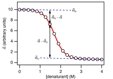
Figure 1: Extrapolation procedure for estimating $\overline{\alpha_{N}}$ and $\overline{\alpha}_{U}$. The white circles and red curve are (synthetic) experimental data. The dashed blue curves are estimates of $\overline{\alpha}_{N}$ and $\overline{\alpha}_{U}$ extrapolated from regions with almost pure $N$ and $U$ into the transition zone. The equilibrium constant is estimated as the ratio between the two distances $\overline{\alpha}_{N}-\overline{\alpha}$ and $\overline{\alpha}-\overline{\alpha}_{U}$. The curves were simulated using Eqs. (24), (25) and (26) with $\overline{\alpha}_{N,0}$ = 10, $\beta_{N}$ = -0.05 M^-1, $\overline{\alpha}_{U,0}$ = 1, $\beta_{N}$ = -0.05 M^-1, $\Delta_{r}G_{U}^{\mathrm{H_{2}O}}$ = 16.9 kJ mol^-1, $m$ = 10 kJ mol^-1 M^-1 and $T$ = 298 K. A script used to generate the synthetic data is available at https://github.com/KULL-Centre/papers/tree/master/2020/stability-lindorff-teilum

In practice one often starts out with the protein as almost pure $N$ (native protein, $p_{N}\approx 1$). As can be seen from Eq. (4) this will in general mean that a measurement of $\overline{\alpha}$ is a measurement of $\overline{\alpha}_{N}$. The reason for this is that for most choices of $\alpha$ the order of magnitude of $\overline{\alpha}_{N}$ and $\overline{\alpha}_{U}$ are the same — we are measuring rather small differences. Therefore one needs to perturb the system by varying one of $T$, $P$ or $\xi$ in order to get reasonable population of both states. This gives several new problems the first one being that only $\overline{\alpha}$ is experimentally accessible. Therefore one needs to use the extrapolation procedure just outlined. The next problem is that the conditions under which $K$ can be estimated are not usually the same as those where the estimate is wanted. An example could be that one has to raise the temperature to $50^{\circ}$C in order to get significant amounts of $N$ and $U$ at the same time, but an estimate of $K$ is needed at $25^{\circ}$C. The solution to this problem is again extrapolation. In general one assumes or knows the functional dependence of $K$ on the perturbing variable either from theory or from previous experiments. This dependence is then used to fit the data in the transition region and thereby provides a way of extrapolating to the conditions where $K$ is needed.

The procedure outlined above was formalized by Santoro and Bolen, (1988) who suggested (focusing on denaturant-induced unfolding) that Eq. (6) is rearranged to:

$$\overline{\alpha}(T,P,\xi)=\frac{\overline{\alpha}_{N}(T,P,\xi)+\overline{\alpha}_{U}(T,P,\xi)K(T,P,\xi)}{1+K(T,P,\xi)}$$ (7)

and that the experimental data consisting of measurements of $\overline{\alpha}$ as a function of $(T,\ P,\ \xi)$ is fitted to Eq. (7) by a non-linear least-squares procedure, as exemplified in Fig. 1. To implement it in practice, one needs to know or assume a specific functional dependence of $\overline{\alpha}_{N}$, $\overline{\alpha}_{U}$ and $K$ on the perturbing variable(s). As detailed with examples below, these dependencies may sometimes come from basic thermodynamic theory, but also often contain some phenomenological component. Using these functional dependencies and the parameters estimated in the fitting procedure one can evaluate $K$ at the desired value of the perturbing parameter. Although this procedure is more rigorous than using individual extrapolations for $\overline{\alpha}_{N}$, $\overline{\alpha}_{U}$ and $K$ it must be stressed that the procedure of evaluating $K$ using the fitted parameters may still be an extrapolation in practice. The procedure itself does not change the fact that it is in general extremely difficult to get precise estimates of $K$ in regions where $p_{N}$ is either 0 or 1. How the functional dependencies of $\overline{\alpha}_{N}$, $\overline{\alpha}_{U}$ and $K$ should be when the perturbing variable is $\xi$ (denaturant induced unfolding) or $T$ (heat or cold induced unfolding) is discussed in the sections below.

To summarize the whole procedure:

1. Choose some physical or chemical observable $\alpha$ that can be measured, and which differ in $N$ and $U$.

2. Perturb the system by changing one or more of the variables $T$, $P$ and $\xi$ in order to explore most of the region of $p_{U}$ from 0 to 1.

3. Measure $\alpha$ under all these conditions.

4. Plot $\overline{\alpha}$ as a function of the perturbing variable(s).

5. Find functional dependencies of $\overline{\alpha}_{N}$, $\overline{\alpha}_{U}$ and $K$ on the perturbing variable(s).

6. Estimate the unknown parameters in these functions, generally by non-linear least-squares regression of the data to Eq. (7).

7. Estimate $K$ at the value of $T$, $P$ and $\xi$ where it is needed.

Denaturant induced unfolding

Denaturants are compounds that are capable of destabilizing the native structure of proteins relative to an unfolded or denatured ensemble of configurations. Two compounds in particular, urea and guanidine hydrochloride (GdnHCl), are extensively used to study protein stability and folding. Adding a denaturant in an adequately high concentration to a protein solution will in most cases cause unfolding of the protein. In the case of the denaturants urea and GdnHCl, which typically cause unfolding at rather high concentration (often several molar), a special treatment is needed since the high concentrations used require the compounds treated as co-solvents and not simply as additives. In the rest of this text the term denaturant will be used, but for all practical purposes we will have guanidinium salts or urea in mind.

The starting point for the discussion is Eq. (7) and in particular the functional dependence of $K$, $\overline{\alpha}_{N}$ and $\overline{\alpha}_{U}$ on $\xi$, where $\xi$ in this section will be the amount of denaturant present in the system parameterized either via the activity ($a_{denat.}$) or molar concentration ($D$). As discussed above it is necessary to know or assume functional dependencies of the perturbing variables in order to use Eq. (7) for analysing protein stability measurements, and these dependencies will be discussed below.

$K$ as a function of the amount of denaturant

Several models for the effect of denaturants on protein stability and how the dependence on $K$ should be treated have been presented (reviewed in Tanford, (1970); Pace, (1986)). As described below, most current research uses the so-called linear extrapolation method (LEM), where the free energy of unfolding is assumed to depend linearly on the molar concentration of the denaturant. We start, however, our discussion with models that are based on mechanistic ideas, and then show how they are related to the LEM.

The ‘denaturant binding model’ (Brandts, 1964b, ; Aune and Tanford, 1969b, ), uses the notion of linked functions (Wyman,, 1964). The theory describes how the equilibrium constant for a reaction, $N\rightleftarrows U$, will be influenced by the presence of a ligand, $x$, which will bind to $N$ and/or $U$. The reaction studied is the denaturation process and the ligand is the denaturant. The result is that the equilibrium constant for the unfolding reaction, $K_{U}$, is related to the number of denaturant molecules taken up during the reaction, $\Delta\nu$, by:

$$\left(\frac{\partial\ln K_{U}}{\partial\ln a_{denat.}}\right)_{T,\ pH}=\Delta\nu$$ (8)

where $a$ denotes activity. As the name implies, the model implicitly assumes a binding of denaturant molecules to the protein. Assuming there are $n_{U}$ ‘binding sites’ on the denatured (unfolded) protein and $n_{N}$ on the native protein and that each of these binding sites are independent and characterized by an individual intrinsic (microscopic) binding constant, $k_{i}$, standard theory for multiple binding sites (Tanford,, 1961) leads to:

$$K_{U}(a_{denat.})=K_{U,0}\frac{\prod_{i=1}^{n_{U}}(1+k_{i,U}a_{denat.})}{\prod_{i=1}^{n_{N}}(1+k_{i,N}a_{denat.})}$$ (9)

Here $K_{U,0}$ denotes the value of $K_{U}$ in the absence of denaturant. Eq. (9) contains too many unknowns to be estimated from a typical experiment. Therefore further approximations are needed. If all sites on $N$ are considered identical, then all $k_{i,N}=k_{N}$. If also all $k_{i,U}$ are set equal to $k_{U}$ this leads to:

$$K_{U}(a_{denat.})=K_{U,0}\frac{\left(1+k_{U}a_{denat.}\right)^{n_{U}}}{\left(1+k_{N}a_{denat.}\right)^{n_{N}}}$$ (10)

Even this equation with five unknown parameters may be too complicated to analyse using normal denaturation data. The model may be simplified further by assuming that the difference in binding of denaturant to $N$ and $U$ lies in the number of sites and not in the individual affinities to the binding sites. This leads to:

$$K_{U}(a_{denat.})=K_{U,0}\left(1+ka_{denat.}\right)^{\Delta n}$$ (11)

or the equivalent:

$$\Delta_{r}G_{U}(a)=\Delta_{r}G_{U}^{\mathrm{H_{2}O}}-\Delta nRT\ln(1+ka_{denat.})$$ (12)

where $\Delta n=n_{U}-n_{N}$ and $\Delta_{r}G_{U}^{\mathrm{H_{2}O}}=-RT\ln K_{U,0}$. In one study, Aune and Tanford, 1969b studied GdnHCl denaturation of lysozyme and found that the model described the data using $\Delta n=7.8$ and $k=3.0$ indicative of weak binding. Values for $k$ and $\Delta n$ are discussed further in Pace, (1986). On the other hand, Brandts, 1964a ; Brandts, 1964b found that this equation could not explain his data on urea denaturation of chymotrypsinogen.

By replotting the data measured by Aune and Tanford, 1969a ; Aune and Tanford, 1969b , Tanford, (1970, Fig. 8) showed a plot of $\log K_{U}$ vs. GdnHCl concentration. $K_{U}$ was measured in an interval of 2–4 M GdnHCl and showed a linear dependence of $\log K_{U}$ on [GdnHCl]. This prompted Greene and Pace, (1974) to suggest what later became known as the LEM (Pace and Shaw,, 2000) in which $K_{U}$ is related to the amount of denaturant present through the equation:

$$\Delta_{r}G_{U}(D)=\Delta_{r}G_{U}^{\mathrm{H_{2}O}}-mD$$ (13)

In this equation, $D$ is the molar concentration of denaturant and $m$, the so called $m$-value, is the (negative) slope in a $\Delta_{r}G_{U}$ vs. $D$ plot (the convention of defining $m$ as the negative slope ensures that $m$ is a positive quantity). This method, which today has become the standard method (Maxwell et al.,, 2005), is mainly used because of its success in describing experimental data. It is simple and describes $\Delta_{r}G_{U}(D)$ by only two parameters as compared to three in Eq. (12) or five in Eq. (10). The major drawback of the method is that it is not accompanied by a theory, leaving interpretations of the two parameters $\Delta_{r}G_{U}^{\mathrm{H_{2}O}}$ and the $m$-value more difficult. To the extent that it is an accurate phenomenological description of protein denaturation, the fitted values of $\Delta_{r}G_{U}^{\mathrm{H_{2}O}}$ represent accurately the stability of a protein extrapolated to the absence of denaturant. From a mechanistic perspective, it is unclear what the $m$-value represents e.g. in terms of the preferential interaction with unfolded proteins, but further phenomenological observations suggest that it is correlated with the change in solvent accessible surface area during unfolding (Schellman,, 1978; Myers et al.,, 1995; Geierhaas et al.,, 2007).

As discussed above, $\Delta_{r}G_{U}$ can only be determined in a limited interval around zero where both the folded and denatured states have sizable populations. This means that the value of $\Delta_{r}G_{U}^{\mathrm{H_{2}O}}$ in Eq. (13) is an extrapolated value. For most proteins denaturation is observed with $D>1\leavevmode\nobreak\ M$ which means that although $\Delta_{r}G_{U}$ may be a linear function in $D$ when it can be measured, it may still behave differently at lower denaturant concentrations. Therefore Eq. (13) may better be interpreted as a truncated series-expansion of $\Delta_{r}G_{U}$ in $D$ around the value $D_{50}$, which is defined as the value of $D$ which gives $\Delta_{r}G_{U}=0$:

$$\begin{split}\Delta_{r}G_{U}(D)=&\left.\frac{\mathrm{d}\Delta_{r}G_{U}}{\mathrm{d}D}\right|_{D_{50}}\mspace{-18.0mu}(D-D_{50})\ +\ \left.\frac{\mathrm{d}^{2}\Delta_{r}G_{U}}{\mathrm{d}D^{2}}\right|_{D_{50}}\mspace{-18.0mu}\frac{(D-D_{50})^{2}}{2!}\\ &+\cdots+\ \left.\frac{\mathrm{d}^{n-1}\Delta_{r}G_{U}}{\mathrm{d}D^{n-1}}\right|_{D_{50}}\mspace{-18.0mu}\frac{(D-D_{50})^{n-1}}{(n-1)!}\ +\ R_{n}\end{split}$$ (14)

Assuming the expansion is represented well by the first-order term alone in some sufficient $D$-interval around $D_{50}$ one finds:

$$m \approx-\left.\frac{\mathrm{d}\Delta_{r}G_{U}}{\mathrm{d}D}\right|_{D_{50}}$$ (15)

$$\Delta_{r}G_{U}(D) \approx-m(D-D_{50})$$ (16)

Using these equations, the extrapolated value $\Delta_{r}G_{U}^{\mathrm{H_{2}O}}$ in Eq. (13) is related to $m$ and $D_{50}$ by:

$$\Delta_{r}G_{U}^{\mathrm{H_{2}O}}\approx mD_{50}$$ (17)

assuming that the expansion in Eq. (14) can be approximated well by the truncated form Eq. (16). Other authors define the $m$-value by:

$$m\equiv-\frac{\mathrm{d}\Delta_{r}G_{U}}{\mathrm{d}D}$$ (18)

which in principle leaves the $m$-value as a function of $D$. In the case where Eq. (13) is valid in the whole $D$-interval, these two definitions (equations (15) and (18)) will obviously coincide. There is, however, some evidence to suggest that the slope of $\Delta_{r}G_{U}(D)$-vs-$D$ may not be constant, i.e. the LEM does not hold fully, (Yi et al.,, 1997; Amsdr et al.,, 2019), which may explain why extrapolated values of $\Delta_{r}G_{U}^{\mathrm{H_{2}O}}$ may differ between different denaturants (Moosa et al.,, 2018).

To accommodate different models and to put equations like (13) on a more solid theoretical ground, a general thermodynamic theory for denaturant induced unfolding is needed. This work was begun by Schellman, (1978, 1987, 1990, 1994); Schellman and Gassner, (1996); Schellman, (2002, 2003) who developed a theory for what he called ‘solvent denaturation’. The reader is referred to these papers for a full description, and only the main results and interpretations will be summarized here. The starting point is the denaturant binding model and the theory of multiple binding sites. From a theoretical point of view one criticism of that model is, that it assumes there are binding sites and treats those binding sites in the language of standard thermodynamic binding theory. This may be correct for ligands with high affinity, but for ‘ligands’ like urea or GdnHCl which exert their effect at very high concentration and therefore must be classified as weak binders, the binding theory misinterprets the notion of binding. Or in the words of Schellman, (1987):

The definition of binding then comes into question. If a site is occupied by a denaturant molecule, is it ‘bound’ or not? Thermodynamically, the answer is ‘yes’ only if the binding is in excess of expectation on the basis of solvent composition.

Therefore Schellman starts out to redefine the notion of binding in a thermodynamic formulation. This is done using multicomponent solution thermodynamics (Casassa and Eisenberg,, 1964), statistical mechanic fluctuation theory (Fowler,, 1936) and refining the linkage theory of Wyman, (1964) to include weakly binding ligands. The observation is that using this new general notion of binding, almost all the equations of standard binding theory can be recovered in the same mathematical form but with new interpretations.

Using the Scatchard notation (Scatchard,, 1946) in a molal basis, the chemical potential of component $j$ in the solution is given by:

$$\mu_{j}=\mu_{0j}^{\ominus}+RT\ln(m_{j}/m^{\ominus})+RT\beta_{j}\qquad j=2,3$$ (19)

Here $\mu_{0j}^{\ominus}$ is the chemical potential of the reference state, $m_{j}$ is the molality and $RT\beta_{j}$ is the excess free energy. We here use the notation with $j=1$ for the principal solvent (water), $j=2$: for the protein and $j=3$: for the co-solvent (denaturant). The equations can easily be generalized to more than one co-solvent. With this notation, Eq. (8) then takes the form:

$$\Gamma_{32} \equiv\lim_{m_{2}\to 0}\left(\frac{\partial m_{3}}{\partial m_{2}}\right)_{\mu_{3}}$$ (20)

$$\left(\frac{\partial\ln K_{U}}{\partial\ln a_{3}}\right) =\Delta\Gamma_{32}$$ (21)

where Eq. (20) is the thermodynamic definition of binding and the $\Delta$ in Eq. (21) refers to the difference in this ‘binding’ between the native and the denatured states. Casassa and Eisenberg, (1964) have shown, that $\Gamma_{23}$, apart from a negligible term, is the binding quantity measured in equilibrium dialysis; if one mole of protein is added at one side of the dialysis membrane then $\approx\Gamma_{23}$ moles of co-solvent have to be added in order to keep its chemical potential constant. Eq. (21) shows how the equilibrium constant for a conformational change depends of the thermodynamics of binding/interactions in the two conformations. Although the mathematical form of equations (8) and (21) are the same, they have different interpretations due to the new definition of binding. To look at an example, assume a single site reaction like:

hydrated site + denaturant = site$\cdot$denaturant + water

For this reaction standard binding theory would yield the binding isotherm in Eq. (22) whereas the solvent exchange model yields Eq. (23):

$$\Gamma_{32} =\frac{K\mathrm{[denaturant]}}{1+K\mathrm{[denaturant]}}$$ (22)

$$\Gamma_{32} =\frac{(K^{\prime}-1)\chi_{3}}{1+(K^{\prime}-1)\chi_{3}}$$ (23)

where $K$ is the (molar) equilibrium constant, $\chi_{3}$ is the mole fraction of co-solvent (denaturant) and $K^{\prime}$ is equal to $Kf_{1}/f_{3}$ where $f_{j}$ are activity coefficients on the mole fraction scale. In the standard binding model $K$ will always be positive whereas the effective binding constant in Eq. (23), $K^{\prime}-1$, will be negative for situations with preferential hydration. This is the main result of the model. It can distinguish the concept ‘binding’ from the concept ‘occupation’ and gives a way of analysing this new definition of binding. Occupation within an area (a site) on a protein, only constitutes binding if the co-solvent is occupying that area more than would be predicted from solvent composition alone.

Schellman’s solvent denaturation model leads to a well-defined theory that links denaturant concentrations (or activities and mole fractions) to preferential binding and thus how a folding equilibrium might be affected. Nevertheless, the resulting equations do not directly lead to something like the LEM, which is generally assumed to describe experiments rather well. Through a number of assumptions Schellman, (1987) arrives at an effective LEM where $\Delta_{r}G_{U}$ is a linear function of denaturant mole fraction, but this model is not commonly used to describe stability measurements. Defining $\beta_{23}=(\partial\beta_{2}/\partial m_{3})$ (see also Eq. (19)) and letting the $\Delta$ operator define a difference between the unfolded and native state, the task of showing the validity of a LEM is equivalent to showing that $\Delta\beta_{23}$ is linear in denaturant concentration.

In theory there are no reasons why a LEM theory should use the molarity of denaturant instead of other concentration scales. To address this question Schellman, (1990) tested linear extrapolations of $\Delta_{r}G_{U}$ in activity, molarity and molality for four proteins. The extrapolated value for $\Delta_{r}G_{U}^{\mathrm{H_{2}O}}$ was compared to that estimated from calorimetric experiments. The result was that the estimate using molarity and molality had the best agreement with the calorimetric estimate. Linearity of the plots were tested with a $\chi^{2}$ test and showed that overall, the molarity scale gave plots which were most linear, providing a practical argument why the LEM is formulated as it is.

To summarize this discussion, we note that standard protein denaturation experiments contain relatively little information about the thermodynamics of unfolding. This in turn implies that only a few parameters can be extracted, and so simple models and equations are generally used. Of the equations presented, ‘the linear extrapolation method’, as presented in equations (13) and (16), has been the most successful. Indeed, even with only two parameters, the LEM can show substantial parameter correlation during non-linear regression (Lindorff-Larsen,, 2019). At the moment there is no good theoretical explanation why these simple equations seem to describe most of the protein denaturation data so well. The solvent exchange model is a big step towards such an explanation, but presumably new types of experiments have to be designed in order to assign values to the parameters in the model. Analysis of enzyme kinetics in the presence of urea (Wu and Wang,, 1999) have provided additional information regarding interaction between proteins and denaturants. Also, extensions of the solvent exchange model have been proposed (Amsdr et al.,, 2019), but are not discussed further here.

$\overline{\alpha}_{N}$ and $\overline{\alpha}_{U}$ as functions of denaturant concentration

We now return to the overall strategy as described in the introduction and captured in Eq. (7). We remind ourselves that we not only need a parametric model for how the free energy of unfolding (or $K(T,P,\xi)$) depends on the solvent composition ($\xi$) (such as the LEM described above), but also need to model how the value of the experimental observable ($\overline{\alpha}$) varies in the two states.

How the average value of the observable $\alpha$ in states $N$ and $U$ depends on the the solvent composition $\xi$ (e.g. the denaturant concentration), will of course depend on which observable has been chosen. In general there are no good theories (like thermodynamics) to use when one looks for the required functional dependencies. For this reason one will in general be satisfied by empirically determined functions. For fluorescence and absorption spectroscopy Schmid, (1997) provides plots of the absorption and fluorescence free tyrosine and tryptophan as a function of denaturant concentration (urea: 0–8.5 M, GdnHCl: 0–7 M). In the cases where an effect is observed, there is an increase in absorption/fluorescence. The results are summarized in Table 1.

Table 1: Effect of denaturants on tyrosine and tryptophan absorption and fluorescence. Values presented are the percent increase in absorption/fluorescence when going from water to a solution containing high denaturant concentration (8.5 M urea or 7.0 M GdnHCl). Data taken from Schmid, (1997), where experimental conditions can be found.

	Tyrosine				Tryptophan
	Absorption		Fluorescence		Absorption		Fluorescence
Urea	50%		20%		20%		40%
GdnHCl	40%		10%		60%		10%

The indicated percentages are the relative increases in absorption/fluorescence intensity. If free tyrosine and tryptophan are good models for protein fluorescence and absorption then these results indicate that a linear function should be adequate for a description of $\overline{\alpha}_{N}$ and $\overline{\alpha}_{U}$ as a function of denaturant concentration. In practice one observes both increases and decreases of fluorescence and absorption in the pre- and post-transition baselines in protein denaturation experiments. This is not surprising since for example the fluorescence intensity of a protein is not simply a sum of the fluorescence from its amino acid constituents in their free states. Other effects like quenching by nearby amino acids or fluorescence resonance energy transfer between tryptophan and tyrosine complicates predictions of how $\overline{\alpha}_{N}$ and $\overline{\alpha}_{U}$ should be modelled (Vivian and Callis,, 2001; Callis,, 2011). Instead, a simple trial and error approach is therefore generally followed. A good starting point will simply be a constant. If the fit is not satisfactory, then using a straight line will in most cases be sufficient. If this is not good enough one should then increase the complexity of the function until an adequately (by some statistical criterion) good fit is obtained. One key problem is that it is only easy to observe deficiencies of the baselines near the ends where the pure folded or unfolded states are populated, but on the other hand, the accuracy of the fit to the thermodynamic model requires that the baselines are also accurate near the transition region.

Linear baselines are used in most cases where denaturant induced unfolding has been measured by CD or fluorescence spectroscopy:

$$\overline{\alpha}_{N}\left(D\right)=\overline{\alpha}_{N,0}+{\beta}_{N}D$$ (24)

$$\overline{\alpha}_{U}\left(D\right)=\overline{\alpha}_{U,0}+{\beta}_{U}D$$ (25)

Inserting these baselines into Eq. (7) and using $K=\exp(-(\Delta rG_{U}^{\mathrm{H_{2}O}}-mD)/RT)$ from Eq. (13) we arrive at:

$$\overline{\alpha}\left(D\right)=\frac{\left(\overline{\alpha}_{N,0}+{\beta}_{N}D\right)+\left(\overline{\alpha}_{U,0}+{\beta}_{U}D\right)\exp{\left(\frac{\Delta_{r}G_{U}^{\mathrm{H_{2}O}}-mD}{RT}\right)}}{1+\exp{\left(\frac{\Delta_{r}G_{U}^{\mathrm{H_{2}O}}-mD}{RT}\right)}}$$ (26)

which is widely accepted as the standard for analysis of denaturant induced protein unfolding (Maxwell et al.,, 2005). Simulated data using this equation are show in Fig. 1.

Heat induced unfolding

In contrast to denaturant induced unfolding there already exists a well tested theoretical apparatus for describing the thermodynamics of heat and cold denaturation of proteins. This model, which is based on standard thermodynamics, has already been discussed extensively in the literature (Privalov,, 1979; Becktel and Schellman,, 1987; Privalov and Gill,, 1988) and will not be repeated here. Only the main features and the standard approximations will be discussed. When heat stability is measured by calorimetry the thermodynamic equations are the only equations needed. On the other hand, if a spectrometric technique like fluorescence is used, one has to use Eq. (7) in order to analyse the data. Here thermodynamics will show you how to setup a function for $K(T)$ but it will not tell you how $\overline{\alpha}_{N}(T)$ and $\overline{\alpha}_{U}(T)$ should be modelled. The question of finding appropriate functions for $K(T)$, $\overline{\alpha}_{N}(T)$ and $\overline{\alpha}_{U}(T)$ are covered in the following two sections.

$K$ as a function of temperature

Below we continue to analyse the thermodynamics of unfolding under the assumption that a two-state description is sufficient. As above, we examine only reversible transitions, and note that in particular thermal unfolding may often be irreversible. For a reversible two-state transition, the relevant equations for discussing the form of $K(T)$ are:

$$\Delta_{r}G_{U}(T) =-RT\ln K_{U}(T)$$ (27)

$$\Delta_{r}G_{U}(T) =\Delta_{r}H_{U}(T)-T\Delta_{r}S_{U}(T)$$ (28)

$$\left(\partial\Delta_{r}H_{U}(T)/\partial T\right)_{P} =\Delta_{r}C_{p,U}(T)$$ (29)

$$\left(\partial\Delta_{r}S_{U}(T)/\partial T\right)_{P} =\Delta_{r}C_{p,U}(T)/T$$ (30)

$$\left(\partial\Delta_{r}G_{U}(T)/\partial T\right)_{P} =-\Delta_{r}S_{U}(T)$$ (31)

$$\left(\mathrm{d}\ln K_{U}^{\ominus}(T)/\mathrm{d}(T^{-1})\right) =-\left(\mathrm{d}\left(\Delta_{r}G_{U}^{\ominus}(T)/RT\right)/\mathrm{d}(T^{-1})\right)$$

$$=-\Delta_{r}H_{U}^{\ominus}(T)/R$$ (32)

One of the defining features when looking at protein denaturation thermodynamics is the large and positive change in heat capacity that is generally found to accompany the unfolding process. This is such a general phenomenon that it has been suggested as the definition of protein denaturation (Lumry and Biltonen,, 1969). The exact reasons for this large $\Delta_{r}C_{p,U}$ are uncertain but they are related to the so called ‘hydrophobic effect’, a term with so many definitions that a full discussion is beyond the scope of the present discussion. We shall therefore simply note that the effect is related to the specific properties of water as a solvent for hydrophobic compounds, and further point the reader to discussions elsewhere (Privalov and Gill,, 1989; Muller,, 1990; Lins and Brasseur,, 1995; Ben-Amotz,, 2016). The effect of having a large $\Delta_{r}C_{p,U}$ can be seen from equations (29) and (30), which show that both the enthalpy and the entropy change will be highly temperature dependent. At most temperatures $|\Delta_{r}G_{U}|$ is much smaller than either of $|\Delta_{r}H_{U}|$ and $|T\Delta_{r}S_{U}|$ (Fig. 2A). This means that the stability of the protein is a small number compared to the two, generally opposing, effects of enthalpy and entropy change.

It is also generally the case that $\Delta_{r}C_{p,U}>|\Delta_{r}S_{U}|$. To see what this means, one can use Eq. (28) instead Eq. (31) to calculate the temperature dependence of $\Delta_{r}G_{U}$:

$$\begin{split}\left(\partial\Delta_{r}G_{U}(T)/\partial T\right)_{P}&=\left(\partial\Delta_{r}H_{U}(T)/\partial T\right)_{P}-\left(\partial(T\Delta_{r}S_{U}(T))/\partial T\right)_{P}\\ &=(\Delta_{r}C_{p,U}(T))-(\Delta_{r}C_{p,U}(T)+\Delta_{r}S_{U}(T))=-\Delta_{r}S_{U}(T)\end{split}$$ (33)

Again, the results show that $\Delta_{r}G_{U}$ is much less temperature dependent than either of $\Delta_{r}H_{U}$ and $T\Delta_{r}S_{U}$ — the increase in denaturation enthalpy by increasing T is almost exactly compensated by an increase in $T\Delta_{r}S_{U}(T)$, leaving only a small temperature effect (of either sign) on $\Delta_{r}G_{U}(T)$.

We proceed by examining the curvature of how $\Delta_{r}G_{U}$ changes as a function of $T$:

$$\left(\partial^{2}\Delta_{r}G_{U}(T)/\partial T^{2}\right)_{P}=-\Delta_{r}C_{p,U}/T$$ (34)

which in general is negative at all relevant temperatures. Generally, there exists some temperature, which we term $T_{S}$, where $\Delta_{r}S_{U}=0$, and so $\Delta_{r}G_{U}$ will be at a maximum at $T_{S}$. Going both up and down from this temperature will decrease the stability ($\Delta_{r}G_{U}$). To sum up, $\Delta_{r}G_{U}$ is a small number compared to $\Delta_{r}H_{U}$ and $T\Delta_{r}S_{U}$ and is much less temperature dependent than either. $\Delta_{r}G_{U}(T)$ has a maximum at $T_{S}$, and below and above this temperature the stability will decrease (Fig. 2B).

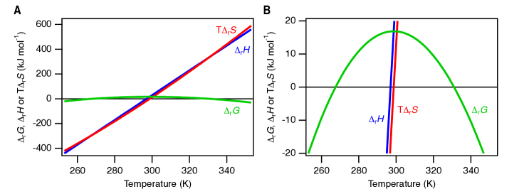
Figure 2: Synthetic data for the temperature dependency of thermodynamic parameters. Blue line: $\Delta_{r}H$. Red line: $T\Delta_{r}S$. Green line: $\Delta_{r}G$. A) shows the full energy interval for $\Delta_{r}H$ and $T\Delta_{r}S$. B) is a close-up on $\Delta_{r}G$. The data were modelled assuming a temperature independent $\Delta_{r}C_{p}$ = 10 kJ mol^-1K^-1, $T_{m}$ = 331 K (58 ^∘C) and $\Delta_{r}H$ = 340 kJ mol^-1 at the melting temperature.

The behaviour described above are those one must bear in mind when choosing some appropriate function $K(T)$. Obviously one cannot neglect the temperature dependence of $\Delta_{r}H_{H}$ and $\Delta_{r}S_{U}$. The simplest function that will include these effects is one using a temperature independent heat capacity change. This approximation will in many cases be adequate for describing experimental data, and only with very precise measurements may it be possible to observe deficiencies arising from it. Assuming $\Delta_{r}C_{p,U}(T)=\Delta_{r}C_{p,U}$ one can integrate equations (29) and (30) and together with Eq. (28) one arrives at:

$$\begin{split}\Delta_{r}G_{U}(T)=&\Delta_{r}H_{U}(T_{0})-T\Delta_{r}S_{U}(T_{0})+\\ &\Delta_{r}C_{p,U}(T-T_{0}-T\ln(T/T_{0}))\end{split}$$ (35)

where $T_{0}$ is some reference temperature. Choosing this temperature as the melting temperature, that is the (highest) temperature where $\Delta_{r}G_{U}(T)=0$ the equation can be reduced to:

$$\Delta_{r}G_{U}(T)= \Delta_{r}H_{U}(T_{m})(1-T/T_{m})+$$

$$\Delta_{r}C_{p,U}(T-T_{m}-T\ln(T/T_{m}))$$ (36)

using that:

$$\Delta_{r}G_{U}(T_{m})= \Delta_{r}H_{U}(T_{m})-T_{m}\Delta_{r}S_{U}(T_{m})=0$$ (37)

Eq. (36) contains three unknown parameters: $\Delta_{r}H_{U}(T_{m})$, $\Delta_{r}C_{p,U}$ and $T_{m}$. If the experimental data does not contain enough information to allow the estimation of these three parameters, then the further (generally poorer) approximation that $\Delta_{r}C_{p,U}=0$ will lead to:

$$\Delta_{r}G_{U}(T)=\Delta_{r}H_{U}(T_{m})(1-T/T_{m})$$ (38)

We note also that if the goal is to determine changes in protein stability at room temperature, then a theoretically-motivated expression can be used to estimate this from changes in $T_{m}$ (Watson et al.,, 2017).

$\overline{\alpha}_{N}$ and $\overline{\alpha}_{U}$ as functions of temperature

With a set of equations in hand that describe how $K$ depends on temperature, we proceed to examine the baselines in heat-induced unfolding experiments. The temperature effect on spectrometric techniques can in general be difficult to predict and will depend on which technique is used. The primary focus in this section will be the temperature dependence of fluorescence intensities, and will exemplify how one may model the baselines using either physical principles or fully empirical approaches.

For both fluorescence (Bushueva et al.,, 1978; Eftink,, 1994) and absorption (Sinha et al.,, 2000) spectroscopy it has been observed that a plot of $\overline{\alpha}$ vs. $T$ can be non-linear even outside the transition region. This effect must be incorporated into the expressions for $\overline{\alpha}_{N}(T)$ and $\overline{\alpha}_{U}(T)$. At the same time one wants to use as few parameters as possible in Eq. (7). Depending on the quality and amount of baseline data one should (in general) not use more than three and preferably less free parameters for determining each baseline. If one is to incorporate all these preferences into a model of the baseline, this is going to be more difficult than in the case of denaturant effects, which are often described well by constant or linear baselines. In particular one needs a simple model that incorporates non-linear baselines. Below we describe one such a model for the temperature-dependency of protein fluorescence based on Bushueva et al., (1978).

In general the fluorescence intensity, $F$, is given by the expression:

$$F=zI_{abs.}q$$ (39)

where $z$ is a factor that among other things is related to the apparatus, $I_{abs.}$ is the amount of absorbed light and $q$ is the quantum yield — the number of photons emitted per photon absorbed. The starting point for the model we describe is that all temperature dependence of $F$ is modelled to be contained in the temperature dependence of the quantum yield. For a single chromophore, $q$ is related to the rate constants for the emission, $k_{F}$, and the non-emitting processes (first-order or pseudo-first-order), $k_{i}$, by the expression:

$$q=\frac{k_{F}}{k_{F}+\sum k_{i}}$$ (40)

Normalizing all rate constants by $k_{F}$ and grouping the non-radiative processes into temperature dependent $k_{j,T}$ and non-temperature dependent $k_{i,NT}$, Eq. (40) can be rewritten:

$$q(T)=\frac{1}{1+\sum_{i}k_{i,NT}+\sum_{j}k_{j,T}}$$ (41)

The task is then to find some expression for the temperature dependence of $\sum_{j}k_{j,T}$. Bushueva et al. suggests that this can be done by using some general temperature dependence function, $f(T)$, for all $k_{j,T}$:

$$q(T)=\frac{1}{1+\sum_{i}k_{i,NT}+f(T)\sum_{j}k_{j,\,eff}}$$ (42)

Here $\sum_{j}k_{j,T}$ has been split into a the temperature dependent $f(T)$ and the temperature independent $\sum_{j}k_{j,\,eff}$. Finally it is suggested that the form of $f(T)$ is given by the temperature dependence of a diffusion-limited reaction. For such a reaction every formation of an encounter pair leads to a reaction. From Fick’s first law of diffusion and the Einstein-Stokes relationship one can determine that the rate constant for a diffusion-limited reaction is given by (Steinfeld et al.,, 1989):

$$k_{D}\approx\frac{2k_{B}(r_{A}+r_{B})^{2}T}{3r_{A}r_{B}\eta(T)}$$ (43)

where $r_{A}$ and $r_{B}$ are the radii of the two reacting species and $\eta(T)$ is the (temperature dependent) viscosity. Grouping all constants and combining equations (39), (42) and (43) results in:

$$f(T)=\left(p_{1}+p_{2}\ T/\eta(T)\right)^{-1}$$ (44)

where $p_{1}$ and $p_{2}$ are temperature-independent parameters.

The assumption that the temperature effect on $q$ is related to a diffusion limited reaction may be accepted for solvent exposed chromophores where collisional quenching by solvent and solutes is possible. For buried aromatic residues on the other hand, one would expect more complex mechanisms. Although it has been shown in some cases (Gavish and Werber,, 1979; Beece et al.,, 1980) that protein dynamics is coupled to solvent viscosity, the issue is complicated both for folded (Ansari et al.,, 1992) and unfolded (Soranno et al.,, 2012) proteins. Thus, Eq. (44) should perhaps be thought of as an empirical relationship that may in some cases describe the temperature dependence of fluorescence intensities (Lindorff-Larsen and Winther,, 2001). Indeed, another possibility is to use a simple, empiric quadratic equation to capture non-linear effects (Saini and Deep,, 2010; Hamborg et al.,, 2020).

As for denaturant induced protein unfolding, we combine the above to arrive at a final expression that can be used for fitting heat induced protein unfolding measured by a spectrometic method. For the native state (here called $N$) where the aromatic residues are buried in the hydrophobic core of the protein it is often sufficient to use a linear temperature dependence:

$$\overline{\alpha}_{N}\left(T\right)=\overline{\alpha}_{N,T_{ref}}+{\gamma}_{N}\left(T-T_{ref}\right)$$ (45)

For the unfolded state (here called $U$) a linear temperature dependence is typically sufficient if the signal is measured by CD spectroscopy. For a signal measured by fluorescence spectroscopy a quadratic temperature dependence may be used as discussed above:

$$\overline{\alpha}_{U}\left(T\right)=\overline{\alpha}_{U,T_{ref}}+{\gamma}_{1,U}\left(T-T_{ref}\right)+{\gamma}_{2,U}\left(T-T_{ref}\right)^{2}$$ (46)

Inserting Eqs. (45) and (46) in Eq. (7) and using $K=\exp(-\Delta_{r}G_{U}(T)/RT)$ we get:

$$\overline{\alpha}\left(T\right)=\frac{\left(\overline{\alpha}_{N,T_{ref}}+{\gamma}_{N}\Delta T\right)+\left(\overline{\alpha}_{U,T_{ref}}+{\gamma}_{1,U}\Delta T+{\gamma}_{2,U}\Delta T^{2}\right)\exp{\left(\frac{-\Delta_{r}G_{U}(T)}{RT}\right)}}{1+\exp{\left(\frac{-\Delta_{r}G_{U}(T)}{RT}\right)}}$$ (47)

where $\Delta T=T-T_{ref}$ and $\Delta_{r}G_{U}(T)$ given by Eq. (36).

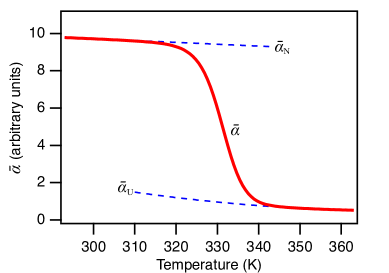
Figure 3: Heat induced unfolding. The red curve is synthetic experimental data. The dashed blue curves are estimates of $\overline{\alpha}_{N}$ and $\overline{\alpha}_{U}$ extrapolated from regions with almost pure $N$ and $U$ into the transition zone. Note that $\overline{\alpha}_{U}$ is curved. The curves were simulated using Eqs. (36), (45), (46) and (47) with $\overline{\alpha}_{N,T_{ref}}$ = 10, $\gamma_{N}$ = -0.01 K^-1, $\overline{\alpha}_{U,T_{ref}}$ = 3, $\gamma_{1,U}$ = -0.05 K^-1, $\gamma_{2,U}$ = 0.00025 K^-2, $\Delta_{r}H(T_{m})$ = 340 kJ mol^-1, $\Delta_{r}C_{p}$ = 10 kJ mol^-1K^-1, $T_{m}$ = 331 K and $T_{ref}$ = 273 K.

Eq. (47) has been used in the literature to analyse temperature unfolding followed in particular by CD spectroscopy (Greenfield,, 2006). In addition to the four or five parameters describing the baselines, three thermodynamic parameters, $\Delta H_{U}(T_{m})$, $\Delta_{r}C_{p,U}$ and $T_{m}$ are obtained from fits to the equation. The values obtained for the thermodynamic parameters depend on the change in the signal in a narrow interval around $T_{m}$. Often both $T_{m}$ and $\Delta H_{U}(T_{m})$ can be determined from the analysis with a reasonable accuracy. However, $\Delta_{r}C_{p,U}$ can generally not be reliably fit from spectroscopic measurements of thermal unfolding (Zweifel and Barrick,, 2001). This parameter divided by $T$ gives the curvature in how $\Delta_{r}G_{U}$ changes with $T$ (Eq. (34)), which in the interval around $T_{m}$ is small compared to the slope of $\Delta_{r}G_{U}$. It is thus generally advised not to fit $\Delta_{r}C_{p,U}=0$ from such data unless the data is of very high quality and reveals clear curvature of $\Delta_{r}G_{U}$. Instead, it is advisable to set $\Delta_{r}C_{p,U}=0$ in Eq. (36), or to use a predicted value (Geierhaas et al.,, 2007), when fitting to Eq. (47). $\Delta_{r}C_{p,U}$ is better determined from a DSC experiment or from a series of CD or fluorescence detected heat induced unfolding experiments where $\Delta_{r}G_{U}$ is changed by adding denaturant (see below).

Differential scanning calorimetry

Differential scanning calorimetry (DSC) is another method which can be used to study protein stability (Freire,, 1995; Johnson,, 2013). A detailed description of how to perform and analyse DSC is outside the scope of this review, but we provide a basic description so that it can be compared to measurements e.g. of thermal unfolding monitored by spectroscopic measurements.

The measured quantity in a DSC experiment is the heat capacity of the system, which thus does not rely on the presence of fluorophores or other probes to measure stability. For this and other reasons DSC complements well the techniques described so far. In a typical DSC setup, two cells, one containing the protein sample and the other a reference, are heated by some specific heating rate (the scan rate). Through an electric feedback loop the temperature difference between the two cells is kept very close to zero. The power used to keep the temperature identical in the two cells is directly related to the difference in heat capacity between the two cells. Since the difference between the two cells is the presence of protein in the sample, one directly measures the heat capacity of the protein.

A hypothetical DSC curve is shown in Fig. 4. Like the other protein unfolding experiments discussed so far, it consists of three regions. First (above 280K) a pre-transition baseline, then a transition region and finally a post-transition region. The major feature in the curve is a large peak associated with the unfolding of the protein. Before this peak, the baseline represents the heat capacity of the native protein. After the peak the baseline represents the heat capacity of the denatured protein. Finally, we note that at the lowest temperatures in the DSC data there is evidence of cold-denaturation in line with the temperature dependency of $\Delta_{r}G$ with these thermodynamic parameters (Fig. 2).

As discussed in the section on heat induced unfolding, $\Delta_{r}C_{p,U}$ for proteins are positive and therefore the post-transition baseline will lie higher than the pre-transition baseline. It is in general a good approximation to assume that $\Delta_{r}C_{p,U}$ is temperature independent, which means that the pre- and post-transition baselines are parallel, although more complex baselines may be used on high quality data (Privalov and Dragan,, 2007).

DSC experiments are generally performed by first making a temperature scan of the background without protein and then subtracting this from a second temperature scan of the protein sample. The measured heat consumption is composed of population-weighted temperature-dependent heat capacities of the folded, $C_{p,N}(T)$ and unfolded, $C_{p,U}(T)$ states (the baseline) and an extra heat contribution, $C_{p,unf}$ resulting from the unfolding of the protein. Using the assumption that the pre- and post-transition baselines are parallel with a common slope, $\gamma$, we get:

$$C_{p,N}(T)=C_{p,N}(T_{m})+\gamma(T-T_{m})$$ (48)

$$C_{p,U}(T)=C_{p,U}(T_{m})+\gamma(T-T_{m})$$ (49)

As the temperature increases the fraction of protein in the native state, $p_{N}$, changes. The heat needed to drive this change is $\Delta_{r}H_{U}$ and the heat capacity associated with unfolding is thus:

$$C_{p,unf}(T)=\Delta_{r}H_{U}(T)\frac{\partial{p_{N}}}{\partial{T}}$$ (50)

For a two-state reaction, the derivative in Eq. (50) can be evaluated by using $p_{N}=1/(1+K(T))$ which gives:

$$\frac{\partial{p_{N}}}{\partial{T}}=\frac{\partial{(1/(1+K(T)))}}{\partial{T}}=\frac{\exp{(-\Delta_{r}G_{U}(T)/RT)}}{(1+\exp{(-\Delta_{r}G_{U}(T)/RT)})^{2}}\frac{\Delta_{r}H_{U}(T)}{RT^{2}}$$ (51)

where $\Delta_{r}H_{U}(T)=\Delta_{r}H_{U}(T)+\Delta_{r}C_{p,U}(T)(T-T_{m})$ and $\Delta_{r}G_{U}(T)$ is given by Eq. (36). Combining Eqs. (48)-(51) gives a final expression for the heat capacity measured in a DSC experiment of a protein following two-state folding:

$$C_{p,meas}(T) =p_{N}C_{p,N}(T)+p_{U}C_{p,U}(T)+\Delta_{r}H_{U}(T)\frac{\partial{p_{N}}}{\partial{T}}$$ (52)

$$=C_{p,N}(T)+(1-p_{N})\Delta_{r}C_{p,U}+\frac{\exp{(-\Delta_{r}G_{U}(T)/RT)}}{(1+\exp{(-\Delta_{r}G_{U}(T)/RT)})^{2}}\frac{(\Delta_{r}H_{U}(T))^{2}}{RT^{2}}$$

In summary, the procedure for measuring protein unfolding by DSC is:

1. A blank scan is performed in order to correct for small differences between the two cells.

2. A temperature scan of the sample vs. reference is performed.

3. The sample is rescanned in order to evaluate whether the unfolding is reversible.

4. The blank scan is subtracted from the sample scan

5. One decides on appropriate functions for the pre- and post-transition baselines and how to join these (Above we used parallel straight lines and a two-state transition).

6. The measured data are fitted to Eq. (52).

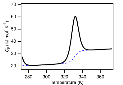
Figure 4: Synthetic data representing a calorimetric scan showing one peak centred at 331 K (58 ^∘C) corresponding to the heat unfolding of a protein. At temperatures below 280 K the beginning of a cold denaturation transition is just appearing. The black curve represents the synthetic experimental data. The blue curve is the baseline. The curve was simulated using Eq. (52) with the parameters $\Delta_{r}H(T_{m})$ = 340 kJ mol^-1, $\Delta_{r}C_{p,U}$ = 10 kJ mol^-1K^-1, $T_{m}$ = 331 K and with a slope of both the pre- and post-transition baselines of 0.04 kJ mol^-1K^-2.

In Fig. 4 we have used a simple two-state model to connect the two parallel baselines according to the amount of native and denatured protein present at that temperature (Takahashi and Sturtevant,, 1981). As mentioned above, the unfolding behaviour may be more complex and require other models for the baselines and non-two-state models to describe the unfolding reaction (Seelig and Schönfeld,, 2016). Because the choice of baselines are model dependent, they may affect the interpretation of the data. For example, it has been shown that different choices of baselines may affect whether a system is thought to behave like a two-state system or not (Zhou et al.,, 1999).

Combining denaturant and heat induced unfolding

So far we have derived expressions for how the observable $\overline{\alpha}$ changes with temperature at a constant denaturant concentration (Eq. (26)) and how it changes with denaturant concentration at a constant temperature (Eq. (47)). If heat induced unfolding of a protein is measured at a series of different denaturant concentrations, we need to extend the formalism to allow for a combined global analysis of all the data. The procedure is the same as we used above with the addition that we need to find expressions for how the parameters $K$, $\overline{\alpha}_{N}$ and $\overline{\alpha}_{U}$ vary when both $T$ and $D$ are changed (Zweifel and Barrick,, 2002; Hamborg et al.,, 2020).

$K$ as a function of denaturant and temperature

The task here is to find an expression for $K_{U}\left(T,D\right)$ or $\Delta_{r}G_{U}\left(T,D\right)$. As $\Delta G$ is a state function, we can first evaluate the effect of changing the temperature and then at the new temperature evaluate the effect of changing the denaturant concentration:

$$\Delta_{r}G_{U}\left(T,D\right)=\int_{T_{m}}^{T}\left(\frac{\partial{\Delta_{r}G}_{U}}{\partial T}\right)_{D=0}\mathrm{d}D+\int_{0}^{D}\left(\frac{\partial{\Delta_{r}G}_{U}}{\partial D}\right)_{T}\mathrm{d}T$$ (53)

As our reference point we have chosen $T=T_{m}$ and $D=0$. From our previous discussion we have the solutions to these two integrals from Eq. (36) and Eq. (13), respectively, which give:

$$\Delta_{r}G_{U}\left(T,D\right)=\Delta_{r}H_{U}\left(T_{m}\right)\left(1-T/T_{m}\right)+\Delta_{r}C_{p,U}\left(T-T_{m}-T\ln\left(T/T_{m}\right)\right)-m\left(T\right)D$$ (54)

where $T_{m}$ and $\Delta_{r}C_{p,U}$ are the values at $D=0$. As discussed above we assume that $\Delta_{r}C_{p,U}$ is independent of temperature. The first integral is calculated at $D=0$ and therefore it is not necessary to know how $\Delta_{r}C_{p,U}$ or $T_{m}$ varies with $D$. The second integral is evaluated at the temperature $T$ and we need to know the temperature dependence of $m$. In the LEM, $m$ is itself a change in free energy and is expected to have a temperature dependence similar to Eq. (36) (Chen and Schellman,, 1989; Neira and Gómez,, 2004),

$$m\left(T\right)=m_{\Delta H_{i}}\left(T_{ref}\right)\left(1-T/T_{ref}\right)+m_{\Delta C_{p,i}}\left(T-T_{ref}-T\ln\left(T/T_{ref}\right)\right)$$ (55)

where $m_{\Delta H_{i}}$ and $m_{\Delta C_{p,i}}$ are the enthalpy and heat capacity associated with the preferential interaction of denaturant with the unfolded state at the reference temperature $T_{ref}$. Several studies have determined $\Delta_{r}G_{U}\left(D\right)$ at multiple temperatures from denaturant induced unfolding experiments and consequently been able to evaluate the temperature dependence of $m$. As far as we are aware, curvature in $m(T)$ has only been observed in a single case (Zweifel and Barrick,, 2002) suggesting that $m_{\Delta C_{p,i}}$ in general is very small. The variation of $m$ with $T$ is overall small, and in some cases $m$ was approximated to be independent of temperature (Chen and Schellman,, 1989; Agashe and Udgaonkar,, 1995; Hollien and Marqusee,, 1999; Hamborg et al.,, 2020). In other cases, however, $m$ decreases linearly with temperature (Makhatadze and Privalov,, 1992; Nicholson and Scholtz,, 1996; DeKoster and Robertson,, 1997; Felitsky and Record,, 2003; Neira and Gómez,, 2004; Amsdr et al.,, 2019) and can be approximated by:

$$m\left(T\right)=m_{\Delta H_{i}}\left(T_{ref}\right)\left(1-T/T_{ref}\right)$$ (56)

Depending on how $m$ varies with $T$, four to six parameters are thus needed to describe $\Delta_{r}G_{U}\left(T,D\right)$.

$\overline{\alpha}_{N}$ and $\overline{\alpha}_{U}$ as functions of denaturant and temperature

Taking the outset from Eqs. (24), (25), (45) and (46) we know how the pre- and post-transition baselines change with denaturant at constant temperature, and how they change with temperature at constant denaturant. The question now is if the slopes of the baselines in the denaturant dimension are temperature dependent or if the slopes of the baselines in the temperature dimension are denaturant dependent. If we assume a linear change of the slopes, we can express the plane $\overline{\alpha}_{i}(T,D)$ for state $i$ as:

$$\overline{\alpha}_{i}\left(T,D\right) =\overline{\alpha}_{i}\left(T_{ref},0\right)+\left({\beta_{i}}+{\beta^{\prime}_{i}}{\Delta}T\right)D+\left({\gamma_{i}}+{\gamma^{\prime}_{i}}D\right){\Delta}T$$ (57)

$$=\overline{\alpha}_{i}\left(T_{ref},0\right)+{\beta_{i}}D+{\gamma_{i}}{\Delta}T+\left({\beta^{\prime}_{i}}+{\gamma^{\prime}_{i}}\right)D{\Delta}T$$

where $\Delta T=\left(T-T_{ref}\right)$. Only few studies in the literature have fitted the pre- and post-transition planes, and to our knowledge in none of these the last $D{\Delta}T$-dependent term was included to obtain satisfactory fits of the experimental data (Nicholson and Scholtz,, 1996; Hollien and Marqusee,, 1999; Neira and Gómez,, 2004; Hamborg et al.,, 2020). We thus proceed by assuming that the $D{\Delta}T$ crossterm is negligible, that the pre-transition plane increases linearly with both $T$ and $D$ (Eqs. (24) and (45)) and that the post-transition plane increases linearly with $D$ (Eq. (25)) and quadratically with $T$ (Eq. (46)). Combining all this with Eqs. (7), (13) and (36) we get an expression to explain and fit a spectrometric signal for protein unfolding in the two-dimensional $(T,D)$ space:

$$\overline{\alpha}\left(T,D\right)=\frac{\left(\overline{\alpha}_{N,0,T_{ref}}+{\beta_{N}}D+{\gamma_{N}}\Delta T\right)+\left(\overline{\alpha}_{U,0,T_{ref}}+{\beta_{U}}D+{\gamma_{1,U}}\Delta T+{\gamma_{2,U}}\Delta T^{2}\right)\exp{\left(\frac{-\Delta_{r}G_{U}(T,D)}{RT}\right)}}{1+\exp{\left(\frac{-\Delta_{r}G_{U}(T,D)}{RT}\right)}}$$ (58)

where $\overline{\alpha}_{i,0,T_{ref}}$ is the spectroscopic signal at $T_{ref}$ in the absence of denaturant, $\Delta T=T-T_{ref}$ and $\Delta_{r}G_{U}(T,D)$ given by Eq. (54). Such two-dimensional unfolding experiments have been used to study the stability of very stable designed proteins (Jacobs et al.,, 2016) and for the analyses of variants with widely different stabilities (Zutz et al.,, 2020). Examples of series of unfolding curves in both the temperature and denaturant dimension are shown in Fig. 5.

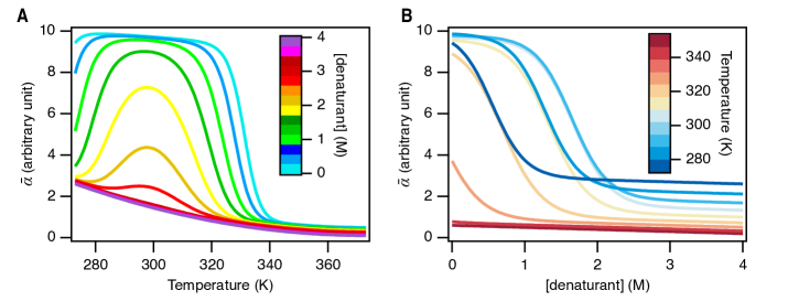
Figure 5: Combined temperature and denaturant induced unfolding. (A) Synthetic temperature unfolding curves at denaturant concentration from 0 to 4 M as indicated by the colour scale. (B) Synthetic denaturant unfolding curves at temperatures from 273 K to 353 K as indicated by the colour scale. The curves were simulated using Eqs. (54) and (58) with $\overline{\alpha}_{N,0,T_{ref}}$ = 10, $\beta_{N}$ = -0.05 M^-1, $\gamma_{N}$ = -0.01 K^-1, $\overline{\alpha}_{U,0,T_{ref}}$ = 3, $\beta_{U}$ = -0.01 M^-1, $\gamma_{1,U}$ = -0.05 K^-1, $\gamma_{2,U}$ = 0.00025 K^-2, $\Delta_{r}H(T_{m})$ = 340 kJ mol^-1, $\Delta_{r}C_{p}$ = 10 kJ mol^-1K^-1, $T_{m}$ = 331 K and $T_{ref}$ = 273 K.

Equilibrium two-state folding

The discussions above generally assume a two-state behaviour, and we have shown how any transition may formally be treated as such, at least in equilibrium experiments. It is, however, also clear that if the system does not behave like a two-state system, but is treated as such, the baselines would have highly non-trivial shapes. This is clear from Eq. (3) which show that unless the subpopulations within each state behave smoothly as a function of a perturbing variable (e.g. temperature) then $\overline{\alpha}_{N}$ and $\overline{\alpha}_{U}$ could be highly non-linear. Thus, it becomes important to consider how much the system behaves more like a thermodynamic system with two separate states, and where the properties of these states are only mildly dependent on the conditions so that they can be considered mostly fixed. This in turn highlights the baselines as potential dumping ground for errors that arise when fitting a multi-state transition to a two-state model, and hence again highlights the importance of sensible choices of baselines and examining how well they fit the data.

Focussing on equilibrium properties, a number of tests have been put forward to address the issue of ‘two-state or not’ (Lumry et al.,, 1966). These tests include the analysis of the temperature dependence of thermodynamic parameters, estimation of parameters using several independent techniques and perhaps the most well-known test of all, the ‘calorimetric criterion’. This criterion states that for a two-state reaction, the unfolding reaction-enthalpy which is obtained by integrating the area between a DSC peak and the merged baselines, should be identical to the enthalpy obtained from the van’t Hoff equation (Eq. (32)) and the temperature dependence of the equilibrium constant determined in the same experiment. It has been shown (Zhou et al.,, 1999) that for any DSC experiment, the calorimetric criterion can be fulfilled by some ‘clever’ choice of baseline. Indeed, this is not just a philosophical issue, as evidenced by the substantially different interpretations of equilibrium unfolding experiments depending in part of the choices of baselines and models (Sadqi et al.,, 2006; Ferguson et al.,, 2007; Zhou and Bai,, 2007; Sadqi et al.,, 2007).

Conclusions

We have here reviewed theory, equations and approaches to study protein stability by experiments. Rather than being comprehensive, we have focused on linking the fundamental properties of molecules with experimental observables. We have focused on equilibrium folding experiments of reversible folding, and discussed general procedures for thinking about these in terms of states, average properties within states, and perturbing the populations of these states by e.g. denaturants or temperature. This procedure involves two key steps. First, one needs to model how the relative population of the states change as a function of the perturbing variable(s), and we have discussed this extensively for denaturants and temperature. Second, because the states are themselves ensembles, and because the spectroscopic probes are sensitive to the conditions, there can be changes to the signals even within the states making it important also to model the baselines. In most current analyses of experiments, standard choices are made for these steps. E.g. nearly all denaturant-induced unfolding experiments are modelled using the LEM for the stability and linear baselines for fluorescence or CD spectroscopy. We hope, however, the reader will have learnt more about the origin, assumptions and potential pitfalls that are involved in such approaches.

References

- Agashe and Udgaonkar, (1995) Agashe, V. R. and Udgaonkar, J. B. (1995). Thermodynamics of Denaturation of Barstar: Evidence for Cold Denaturation and Evaluation of the Interaction with Guanidine Hydrochloride. Biochemistry, 34(10):3286–3299.
- Amsdr et al., (2019) Amsdr, A., Noudeh, N. D., Liu, L., and Chalikian, T. V. (2019). On urea and temperature dependences of m-values. The Journal of chemical physics, 150(21):215103.
- Ansari et al., (1992) Ansari, A., Jones, C. M., Henry, E. R., Hofrichter, J., and Eaton, W. A. (1992). The role of solvent viscosity in the dynamics of protein conformational changes. Science, 256(5065):1796–1798.
- (4) Aune, K. C. and Tanford, C. (1969a). Thermodynamics of the denaturation of lysozyme by guanidine hydrochloride. i. dependence on ph at 25. Biochemistry, 8(11):4579–4585.
- (5) Aune, K. C. and Tanford, C. (1969b). Thermodynamics of the denaturation of lysozyme by guanidine hydrochloride. ii. dependence on denaturant concentration at 25c. Biochemistry, 8(11):4586–4590.
- Becktel and Schellman, (1987) Becktel, W. J. and Schellman, J. A. (1987). Protein stability curves. Biopolymers: Original Research on Biomolecules, 26(11):1859–1877.
- Beece et al., (1980) Beece, D., Eisenstein, L., Frauenfelder, H., Good, D., Marden, M., Reinisch, L., Reynolds, A., Sorensen, L., and Yue, K. (1980). Solvent viscosity and protein dynamics. Biochemistry, 19(23):5147–5157.
- Ben-Amotz, (2016) Ben-Amotz, D. (2016). Water-mediated hydrophobic interactions. Annual review of physical chemistry, 67:617–638.
- (9) Brandts, J. F. (1964a). The thermodynamics of protein denaturation. i. the denaturation of chymotrypsinogen. Journal of the American Chemical Society, 86(20):4291–4301.
- (10) Brandts, J. F. (1964b). The thermodynamics of protein denaturation. ii. a model of reversible denaturation and interpretations regarding the stability of chymotrypsinogen. Journal of the American Chemical Society, 86(20):4302–4314.
- Brandts, (1969) Brandts, J. F. (1969). Conformational transitions of proteins in water and in aqueous mixtures. In Timasheff, S. and Fasman, G., editors, Structure and stability of biological macromolecules, volume 2, chapter 3, pages 213–290. Marcel Dekker, New York.
- Bushueva et al., (1978) Bushueva, T., Busel, E., and Burstein, E. (1978). Relationship of thermal quenching of protein fluorescence to intramolecular structural mobility. Biochimica et Biophysica Acta (BBA)-Protein Structure, 534(1):141–152.
- Callis, (2011) Callis, P. R. (2011). Predicting fluorescence lifetimes and spectra of biopolymers. In Methods in enzymology, volume 487, pages 1–38. Elsevier.
- Casassa and Eisenberg, (1964) Casassa, E. F. and Eisenberg, H. (1964). Thermodynamic analysis of multicomponent solutions. Adv Protein Chem, 19:287–395.
- Chen and Schellman, (1989) Chen, B. L. and Schellman, J. A. (1989). Low-temperature unfolding of a mutant of phage T4 lysozyme. 1. Equilibrium studies. Biochemistry, 28(2):685–691.
- DeKoster and Robertson, (1997) DeKoster, G. T. and Robertson, A. D. (1997). Calorimetrically-derived parameters for protein interactions with urea and guanidine-HCl are not consistent with denaturant m values. Biophysical Chemistry, 64(1-3):59–68.
- Eftink, (1994) Eftink, M. R. (1994). The use of fluorescence methods to monitor unfolding transitions in proteins. Biophysical journal, 66(2):482–501.
- Felitsky and Record, (2003) Felitsky, D. J. and Record, M. T. (2003). Thermal and Urea-Induced Unfolding of the Marginally Stable Lac Repressor DNA-Binding Domain: A Model System for Analysis of Solute Effects on Protein Processes. Biochemistry, 42(7):2202–2217.
- Ferguson et al., (2007) Ferguson, N., Sharpe, T. D., Johnson, C. M., Schartau, P. J., and Fersht, A. R. (2007). Analysis of ‘downhill’ protein folding. Nature, 445(7129):E14–E15.
- Fowler, (1936) Fowler, R. H. (1936). Statistical thermodynamics. Cambridge University Press, 2 edition.
- Freire, (1995) Freire, E. (1995). Differential scanning calorimetry. In Shirley, B., editor, Protein stability and folding, pages 191–218. Humana Press.
- Gavish and Werber, (1979) Gavish, B. and Werber, M. (1979). Viscosity-dependent structural fluctuations in enzyme catalysis. Biochemistry, 18(7):1269–1275.
- Geierhaas et al., (2007) Geierhaas, C. D., Nickson, A. A., Lindorff-Larsen, K., Clarke, J., and Vendruscolo, M. (2007). Bppred: A web-based computational tool for predicting biophysical parameters of proteins. Protein Science, 16(1):125–134.
- Greene and Pace, (1974) Greene, R. F. and Pace, C. N. (1974). Urea and guanidine hydrochloride denaturation of ribonuclease, lysozyme, -chymotrypsin, and -lactoglobulin. Journal of Biological Chemistry, 249(17):5388–5393.
- Greenfield, (2006) Greenfield, N. J. (2006). Using circular dichroism collected as a function of temperature to determine the thermodynamics of protein unfolding and binding interactions. Nature Protocols, 1(6):2527–2535.
- Hamborg et al., (2020) Hamborg, L., Horsted, E. W., Johansson, K. E., Willemoës, M., Lindorff-Larsen, K., and Teilum, K. (2020). Global analysis of protein stability by temperature and chemical denaturation. Analytical Biochemistry, 605:113863.
- Hollien and Marqusee, (1999) Hollien, J. and Marqusee, S. (1999). A Thermodynamic Comparison of Mesophilic and Thermophilic Ribonucleases H †. Biochemistry, 38(12):3831–3836.
- Jacobs et al., (2016) Jacobs, T., Williams, B., Williams, T., Xu, X., Eletsky, A., Federizon, J., Szyperski, T., and Kuhlman, B. (2016). Design of structurally distinct proteins using strategies inspired by evolution. Science, 352(6286):687–690.
- Johnson, (2013) Johnson, C. M. (2013). Differential scanning calorimetry as a tool for protein folding and stability. Archives of Biochemistry and Biophysics, 531(1-2):100–109.
- Lindorff-Larsen, (2019) Lindorff-Larsen, K. (2019). Dissecting the statistical properties of the linear extrapolation method of determining protein stability. Protein Engineering, Design and Selection, 32(10):471–479.
- Lindorff-Larsen and Winther, (2001) Lindorff-Larsen, K. and Winther, J. R. (2001). Surprisingly high stability of barley lipid transfer protein, ltp1, towards denaturant, heat and proteases. FEBS letters, 488(3):145–148.
- Lins and Brasseur, (1995) Lins, L. and Brasseur, R. (1995). The hydrophobic effect in protein folding. The FASEB journal, 9(7):535–540.
- Lumry and Biltonen, (1969) Lumry, R. and Biltonen, R. (1969). Thermodynamic and kinetic aspects of protein conformations in relation to physiological function. In Timasheff, S. and Fasman, G., editors, Structure and stability of biological macromolecules, volume 2, chapter 2, pages 65–212. Marcel Dekker, New York.
- Lumry et al., (1966) Lumry, R., Biltonen, R., and Brandts, J. F. (1966). Validity of the ‘two-state’ hypothesis for conformational transitions of proteins. Biopolymers: Original Research on Biomolecules, 4(8):917–944.
- Makhatadze and Privalov, (1992) Makhatadze, G. I. and Privalov, P. L. (1992). Protein interactions with urea and guanidinium chloride A calorimetric study. Journal of Molecular Biology, 226(2):491–505.
- Maxwell et al., (2005) Maxwell, K. L., Wildes, D., Zarrine-Afsar, A., Rios, M. A. D. L., Brown, A. G., Friel, C. T., Hedberg, L., Horng, J.-C., Bona, D., Miller, E. J., Vallée-Bélisle, A., Main, E. R. G., Bemporad, F., Qiu, L., Teilum, K., Vu, N.-D., Edwards, A. M., Ruczinski, I., Poulsen, F. M., Kragelund, B. B., Michnick, S. W., Chiti, F., Bai, Y., Hagen, S. J., Serrano, L., Oliveberg, M., Raleigh, D. P., Wittung-Stafshede, P., Radford, S. E., Jackson, S. E., Sosnick, T. R., Marqusee, S., Davidson, A. R., and Plaxco, K. W. (2005). Protein folding: Defining a “standard” set of experimental conditions and a preliminary kinetic data set of two-state proteins. Protein Science, 14(3):602–616.
- Miyawaki and Tatsuno, (2011) Miyawaki, O. and Tatsuno, M. (2011). Thermodynamic analysis of alcohol effect on thermal stability of proteins. Journal of bioscience and bioengineering, 111(2):198–203.
- Moosa et al., (2018) Moosa, M. M., Goodman, A. Z., Ferreon, J. C., Lee, C. W., Ferreon, A. C. M., and Deniz, A. A. (2018). Denaturant-specific effects on the structural energetics of a protein-denatured ensemble. European Biophysics Journal, 47(1):89–94.
- Muller, (1990) Muller, N. (1990). Search for a realistic view of hydrophobic effects. Accounts of Chemical Research, 23(1):23–28.
- Myers et al., (1995) Myers, J. K., Nick Pace, C., and Martin Scholtz, J. (1995). Denaturant m values and heat capacity changes: relation to changes in accessible surface areas of protein unfolding. Protein Science, 4(10):2138–2148.
- Neira and Gómez, (2004) Neira, J. L. and Gómez, J. (2004). The conformational stability of the Streptomyces coelicolor histidine‐phosphocarrier protein. European Journal of Biochemistry, 271(11):2165–2181.
- Nicholson and Scholtz, (1996) Nicholson, E. M. and Scholtz, J. M. (1996). Conformational Stability of the Escherichia coli HPr Protein: Test of the Linear Extrapolation Method and a Thermodynamic Characterization of Cold Denaturation †. Biochemistry, 35(35):11369–11378.
- Pace, (1986) Pace, C. N. (1986). [14] determination and analysis of urea and guanidine hydrochloride denaturation curves. In Methods in enzymology, volume 131, pages 266–280. Elsevier.
- Pace and Shaw, (2000) Pace, C. N. and Shaw, K. L. (2000). Linear extrapolation method of analyzing solvent denaturation curves. Proteins: Structure, Function, and Bioinformatics, 41(S4):1–7.
- Privalov and Gill, (1989) Privalov, P. and Gill, S. J. (1989). The hydrophobic effect: a reappraisal. Pure and Applied Chemistry, 61(6):1097–1104.
- Privalov, (1979) Privalov, P. L. (1979). Stability of proteins small globular proteins. In Advances in protein chemistry, volume 33, pages 167–241. Elsevier.
- Privalov and Dragan, (2007) Privalov, P. L. and Dragan, A. I. (2007). Microcalorimetry of biological macromolecules. Biophysical Chemistry, 126(1-3):16–24.
- Privalov and Gill, (1988) Privalov, P. L. and Gill, S. J. (1988). Stability of protein structure and hydrophobic interaction. In Advances in protein chemistry, volume 39, pages 191–234. Elsevier.
- Sadqi et al., (2006) Sadqi, M., Fushman, D., and Munoz, V. (2006). Atom-by-atom analysis of global downhill protein folding. Nature, 442(7100):317–321.
- Sadqi et al., (2007) Sadqi, M., Fushman, D., and Muñoz, V. (2007). Analysis of ‘downhill’ protein folding; analysis of protein-folding cooperativity (reply). Nature, 445(7129):E17–E18.
- Saini and Deep, (2010) Saini, K. and Deep, S. (2010). Relationship between the wavelength maximum of a protein and the temperature dependence of its intrinsic tryptophan fluorescence intensity. European Biophysics Journal, 39(10):1445–1451.
- Santoro and Bolen, (1988) Santoro, M. M. and Bolen, D. (1988). Unfolding free energy changes determined by the linear extrapolation method. 1. unfolding of phenylmethanesulfonyl. -chymotrypsin using different denaturants. Biochemistry, 27(21):8063–8068.
- Scatchard, (1946) Scatchard, G. (1946). Physical chemistry of protein solutions. i. derivation of the equations for the osmotic pressure1. Journal of the American Chemical Society, 68(11):2315–2319.
- Schellman, (1978) Schellman, J. A. (1978). Solvent denaturation. Biopolymers: Original Research on Biomolecules, 17(5):1305–1322.
- Schellman, (1987) Schellman, J. A. (1987). Selective binding and solvent denaturation. Biopolymers: Original Research on Biomolecules, 26(4):549–559.
- Schellman, (1990) Schellman, J. A. (1990). Fluctuation and linkage relations in macromolecular solution. Biopolymers: Original Research on Biomolecules, 29(1):215–224.
- Schellman, (1994) Schellman, J. A. (1994). The thermodynamics of solvent exchange. Biopolymers: Original Research on Biomolecules, 34(8):1015–1026.
- Schellman, (2002) Schellman, J. A. (2002). Fifty years of solvent denaturation. Biophysical chemistry, 96(2-3):91–101.
- Schellman, (2003) Schellman, J. A. (2003). Protein stability in mixed solvents: a balance of contact interaction and excluded volume. Biophysical journal, 85(1):108–125.
- Schellman and Gassner, (1996) Schellman, J. A. and Gassner, N. C. (1996). The enthalpy of transfer of unfolded proteins into solutions of urea and guanidinium chloride. Biophysical chemistry, 59(3):259–275.
- Schmid, (1997) Schmid, F. (1997). Optical spectroscopy to characterize protein conformation and conformational changes. In Protein structure: A practical approach, chapter 11, pages 262–297. Oxford University Press New York.
- Seelig and Schönfeld, (2016) Seelig, J. and Schönfeld, H.-J. (2016). Thermal protein unfolding by differential scanning calorimetry and circular dichroism spectroscopy Two-state model versus sequential unfolding. Quarterly Reviews of Biophysics, 49:e9.
- Sinha et al., (2000) Sinha, A., Yadav, S., Ahmad, R., and Ahmad, F. (2000). A possible origin of differences between calorimetric and equilibrium estimates of stability parameters of proteins. Biochemical Journal, 345(3):711–717.
- Soranno et al., (2012) Soranno, A., Buchli, B., Nettels, D., Cheng, R. R., Müller-Späth, S., Pfeil, S. H., Hoffmann, A., Lipman, E. A., Makarov, D. E., and Schuler, B. (2012). Quantifying internal friction in unfolded and intrinsically disordered proteins with single-molecule spectroscopy. Proceedings of the National Academy of Sciences, 109(44):17800–17806.
- Steinfeld et al., (1989) Steinfeld, J. I., Francisco, J. S., and Hase, W. L. (1989). Chemical kinetics and dynamics, volume 3. Prentice Hall Englewood Cliffs (New Jersey).
- Street et al., (2008) Street, T. O., Courtemanche, N., and Barrick, D. (2008). Protein folding and stability using denaturants. Methods in cell biology, 84:295–325.
- Takahashi and Sturtevant, (1981) Takahashi, K. and Sturtevant, J. M. (1981). Thermal denaturation of streptomyces subtilisin inhibitor, subtilisin bpn’, and the inhibitor-subtilisin complex. Biochemistry, 20(21):6185–6190.
- Tanford, (1961) Tanford, C. (1961). Ionization-linked changes in protein conformation. i. theory. Journal of the American Chemical Society, 83(7):1628–1634.
- Tanford, (1970) Tanford, C. (1970). Protein denaturation. Adv. Protein Chem, 24(1):95.
- Vivian and Callis, (2001) Vivian, J. T. and Callis, P. R. (2001). Mechanisms of tryptophan fluorescence shifts in proteins. Biophysical journal, 80(5):2093–2109.
- Watson et al., (2017) Watson, M. D., Monroe, J., and Raleigh, D. P. (2017). Size-dependent relationships between protein stability and thermal unfolding temperature have important implications for analysis of protein energetics and high-throughput assays of protein–ligand interactions. The Journal of Physical Chemistry B, 122(21):5278–5285.
- Wu and Wang, (1999) Wu, J.-W. and Wang, Z.-X. (1999). New evidence for the denaturant binding model. Protein Science, 8(10):2090–2097.
- Wyman, (1964) Wyman, J. J. (1964). Linked functions and reciprocal effects in hemoglobin: a second look. Advances in protein chemistry, page 223.
- Yi et al., (1997) Yi, Q., Scalley, M. L., Simons, K. T., Gladwin, S. T., and Baker, D. (1997). Characterization of the free energy spectrum of peptostreptococcal protein l. Folding and Design, 2(5):271–280.
- Zhou et al., (1999) Zhou, Y., Hall, C. K., and Karplus, M. (1999). The calorimetric criterion for a two-state process revisited. Protein Science, 8(5):1064–1074.
- Zhou and Bai, (2007) Zhou, Z. and Bai, Y. (2007). Analysis of protein-folding cooperativity. Nature, 445(7129):E16–E17.
- Zutz et al., (2020) Zutz, A., Hamborg, L., Pedersen, L. E., Kassem, M. M., Papaleo, E., Koza, A., Herrgård, M. J., Teilum, K., Lindorff-Larsen, K., and Nielsen, A. T. (2020). A dual-reporter system for investigating and optimizing protein translation and folding in e. coli. bioRxiv.
- Zweifel and Barrick, (2001) Zweifel, M. E. and Barrick, D. (2001). Studies of the ankyrin repeats of the drosophila melanogaster notch receptor. 2. solution stability and cooperativity of unfolding. Biochemistry, 40(48):14357–14367.
- Zweifel and Barrick, (2002) Zweifel, M. E. and Barrick, D. (2002). Relationships between the temperature dependence of solvent denaturation and the denaturant dependence of protein stability curves. Biophysical Chemistry, 101:221–237.