chapter Multiple-merger coalescents
 
Multiple-merger coalescents

FF-sect:intro Two decades ago, $\Lambda$- and shortly later the bigger class of $\Xi$-$n$-coalescents have been introduced and become an active area of mathematical research ever since. These are Markov processes $\Pi^{(n)}=(\Pi^{(n)}_{t})_{t\geqslant 0}$ on the set of partitions of $\{1,\ldots,n\}$. Transitions are mergers of partition blocks. A $\Xi$-$n$-coalescent’s rates are characterised by a finite measure $\Xi$ with positive mass on the simplex

$$\Delta=\{(x_{i})_{i\in\mathbb{N}}:x_{1}\geqslant x_{2}\geqslant\ldots,\sum_{i\in\mathbb{N}}x_{i}\leqslant 1\}.$$

An intuitive way of describing the transitions is via a Poisson construction, see [49, 54]: Transitions are possible at times $t\in[0,\infty)$ that feature a point $(t,x)$ of a Poisson point process on $[0,\infty)\times\Delta$ with intensity $\hskip 0.5pt\mathrm{d}\hskip 0.5ptt\otimes\frac{\Xi^{*}(\hskip 0.5pt\mathrm{d}\hskip 0.5ptx)}{(x,x)}$, where $\Xi^{*}$ is the restriction of $\Xi$ to $\Delta\setminus\{(0,0,\ldots)\}$ and $(x,x):=\sum_{i\in\mathbb{N}}x^{2}_{i}$. At time $t$, consider the ’paintbox’ $x=(x_{1},x_{2},\ldots)$: Each partition block $i$ present at $t$ draws independently a colour $C_{i}$, which paints it with colour $j\in\mathbb{N}$ with $P(C_{i}=j)=x_{j}$ and makes it colourless with $P(C_{i}=0)=1-\sum_{m\in\mathbb{N}}x_{m}$. Merge each set of blocks of the same colour. If $\Xi$ has positive mass on the origin, say $a=\Xi(\{(0,0,\ldots)\})$, also allow additional transitions for each pair of blocks present with transition rate $a$.

Such coalescents allow transitions that are mergers of sets of any number of blocks present into multiple new blocks. If $\Xi$ has only positive mass on the first coordinate of the simplex, only a single set of blocks can be merged into one new block as a transition. This subclass of $\Xi$-$n$-coalescents are called $\Lambda$-$n$-coalescents, $\Lambda$ being the restriction of $\Xi$ to the first dimension of $\Delta$, a finite measure on $[0,1]$.

For any $\Xi$, $\Pi^{(n)}$ almost surely reaches its absorbing state $\{1,\ldots,n\}$ in finite time. For any fixed time $t$, the partition $\Pi^{(n)}_{t}$ of the $\Xi$-$n$-coalescent is exchangeable, i.e. $\sigma(\Pi^{(n)}_{t})\stackrel{{\scriptstyle d}}{{=}}\Pi^{(n)}_{t}$ for any permutation $\sigma$ of $\{1,\ldots,n\}$. This extends to certain non-deterministic times, for instance the partition before absorption in $\{\{1,\ldots,n\}\}$ is exchangeable. Moreover, there exists a Kolmogorov extension $(\Pi_{t})_{t\geqslant 0}$ on the set of partitions of $\mathbb{N}$ so that its restriction to $[n]:=\{1,\ldots,n\}$ is a $\Xi$-$n$-coalescent for any $n\in\mathbb{N}$, see [54, Theorem 2]. $\Pi=(\Pi_{t})_{t\geqslant 0}$ is called a $\Xi$-coalescent. Exchangeability extends to the $\Xi$-coalescent in the sense that any permutation of a finite set $S\subset\mathbb{N}$ does not change the distribution of $\Pi$. A consequence of this is that the limit frequencies $\lim_{n\to\infty}B^{(n)}_{i}(t)/n$ of the partition block sizes $B^{(n)}_{i}(t)$ of the restrictions of $\Pi_{t}$ to $[n]$ (e.g. ordered by sizes) exist almost surely, this is called Kingman’s correspondence (which is essentially de Finetti’s theorem, see e.g. [54, Appendix]). $\Xi$-$n$-coalescents and related models also appear as central objects in other chapters, see the contributions of Birkner and Blath [6], of Kersting and Wakolbinger [34] as well as of Sturm [59] in this volume.

The Poisson construction also shows fundamental differences between different choices of $\Xi$ (respectively $\Lambda$). While choosing $\Lambda=\delta_{0}$ leads to Kingman’s $n$-coalescent, which only allows binary mergers, any $\Xi$ with mass outside of $(0,0,\ldots)$ allows for mergers of more than two blocks (which are the name-giving multiple mergers). If $\frac{\Xi(\hskip 0.5pt\mathrm{d}\hskip 0.5ptx)}{(x,x)}$ is a finite measure, the Poisson point process almost surely only has finitely many points on any set $[0,t]\times\Delta$. For such $\Xi$, the corresponding subclass of coalescent processes are called simple $\Xi$-($n$-)coalescents. If $\sum_{i\in\mathbb{N}}x_{i}\frac{\Xi(\hskip 0.5pt\mathrm{d}\hskip 0.5ptx)}{(x,x)}$ is a finite measure, at least the number of mergers the block containing a fixed $i\in\mathbb{N}$ can participate in is almost surely finite. Corresponding $\Xi$(-$n$)-coalescents are called coalescents with dust. All simple $\Xi$(-$n$)-coalescents are also coalescents with dust. A further property of $\Xi$-coalescents is whether they stay infinite, i.e. which have infinitely many blocks almost surely at any time, or whether they come down from infinity, i.e. they have finitely many blocks at any time $t>0$ almost surely. All $\Xi$-coalescents with dust that do not allow for Poisson points where all blocks are coloured with finitely many colours, i.e. that have $\Xi(\{x\in\Delta:\sum_{i=1}^{k}x_{i}=1\mbox{ for a }k\in\mathbb{N}\})=0$ stay infinite, see e.g. [20, Sect. 3]. The case of $\Xi$-coalescents without dust is more complex, see e.g. [27]. We will need later that the times to absorption of $\Xi$-$n$-coalescents not staying infinite are converging almost surely to a finite limiting variable for $n\to\infty$: this follows from [54, Lemma 31] if the coalescent comes down from infinity. Otherwise, the same lemma shows that $\Xi$ has positive mass on Poisson points that colour all present blocks with finitely many colours. Thus, there is a finite waiting time for such points, which then forces the number of blocks to be finite and subsequently these will merge into absorption after a finite time almost surely.

One can even put this stronger for both cases: Since only finitely many blocks merge, exchangeability ensures that given $n$ large enough, all the blocks of the $\Xi$-coalescent merging at the last collision have at least one individual in the blocks of the $\Xi$-$n$-coalescent. Thus, the height of the $\Xi$-$n$-coalescent is the same as for the $\Xi$-coalescent above a certain (path-dependent) $n_{0}$, if the $\Xi$-coalescent does not stay infinite.

Any $\Xi$-$n$-coalescent also encodes a random ultrametric (labelled) tree with $n$ leaves, where ultrametric means that the path lengths from leaves to root are identical for all leaves. We build this tree from leaves to root: Start with $n$ edges (initially length 0) at the leaves corresponding to the blocks $\{1\},\ldots,\{n\}$ at time 0. Elongate all edges by $l_{1}$, where $l_{1}$ is the waiting time for the first transition of $\Pi^{(n)}$. Then, the edges corresponding to the sets of merged partition blocks of $\Pi^{(n)}$ at this transition are joined in new internal nodes (for $\Xi$-$n$-coalescents, a transition may consist of multiple simultaneous mergers). Start a new edge at each newly introduced node (length 0) and elongate again all branches not yet connected to two nodes for $l_{2}$, the waiting time until the next transition of the $n$-coalescent. The new edges represent the blocks formed at the transition at time $l_{1}$. Then, join all edges (not yet connected to two nodes) in a new node that correspond to the set(s) of blocks merged at the second transition and start again new edges (length 0) from these nodes (representing the newly formed blocks at the second transition). Repeat this until all blocks are merged, which corresponds to the root of the tree.

Kingman’s $n$-coalescent has been introduced by Kingman [35, 36] as approximating the genealogical tree of a sample of $n$ individuals of a haploid Wright–Fisher model with (large) population size $N$. Here, the discrete genealogy is defined by recording the partitions of $\{1,\ldots n\}$ corresponding to which sets of individuals in $\{1,\ldots n\}$ have the same ancestor $r$ generations backwards from the time of sampling for all $r\in\mathbb{N}$. This partition-valued process $(\mathcal{R}^{(N)}_{r})_{r\in\mathbb{N}}$ then converges for $N\to\infty$ when time is rescaled, i.e.

(1.0.1) $$\big{(}\mathcal{R}^{(N)}_{\lceil c^{-1}_{N}t\rceil}\big{)}_{t\geqslant 0}\stackrel{{\scriptstyle d}}{{\to}}\Pi^{(n)},$$

where $\Pi^{(n)}$ is Kingman’s $n$-coalescent $\Pi^{(n),\delta_{0}}$ and $c_{N}$ is the probability that two individuals drawn at random from the same generation have the same parent in the reproduction model, so $c_{N}=N^{-1}$ in the Wright–Fisher model. For any $\Xi$-$n$-coalescent $\Pi^{(n),\Xi}$, there exists a series of Cannings models, i.e. haploid reproduction models of a population of fixed size $N$ in any generation with exchangeable offspring numbers (i.i.d. across generations), so that Eq. (1.0.1) holds for $\Pi^{(n)}=\Pi^{(n),\Xi}$, see [44].

While the Wright–Fisher model is a staple model in population genetics, the standard model of a neutrally evolving fixed-size population, the Cannings models leading to other $\Xi$-$n$-coalescents are used more rarely. This is inherited by the coalescent process limits. The prevalence of Kingman’s $n$-coalescent also stems from its robustness: If a series of Cannings models with $c_{N}\to 0$ and non-extreme variance in offspring numbers across individuals satisfies Eq. (1.0.1) for some limit process $\Pi^{(n)}$, then $\Pi^{(n)}$ is Kingman’s $n$-coalescent, see [43]. Such models include the Moran model, where one random individual has two, a different one no and all others one offspring.

However, there is growing evidence that for certain populations, $\Xi$-$n$-coalescents are fitting better as genealogy models. Necessarily, as discussed above, these need to be populations where ancestors are shared by many offspring. For instance, a biological mechanism leading there is sweepstake reproduction, i.e. one “lucky” individual/genotype produces considerably more offspring on the coalescent time scale than the rest of the (potential) parents [25]. An example would be type III survivorship in marine species, where individuals reproduce with large offspring numbers, but high early-life mortality keeps the population size constant. This has been modelled in [55] as sampling $N$ actual offspring from the potential offspring (in reality offspring dying in an early life stage) of $N$ parents given by i.i.d. $(\nu^{(N)}_{1},\ldots,\nu^{(N)}_{N})$ with heavy tails, i.e. $P(\nu_{1}\geqslant k)\sim Ck^{-\alpha}$. If $\alpha\in[1,2)$, the limit in Eq. 1.0.1 from this model is a Beta-$n$-coalescent, i.e. a $\Lambda$-$n$-coalescent with $\Lambda=Beta(2-\alpha,\alpha)$ being a Beta distribution. These coalescents have no dust, and come down from infinity for $\alpha>1$ but stay infinite for $\alpha=1$. While the Beta-$n$-coalescents model haploid sweepstake reproduction, diploid reproduction leads to a $\Xi$-$n$-coalescent limit, the Beta-$\Xi$-$n$-coalescent, see [9, 8].

In [16], a different haploid model of sweepstake reproduction in a population of fixed size $N$ was introduced: In a Moran model, with small probability $N^{-\gamma}$, $\gamma>0$, the single individual having two offspring instead has $U=\lceil N\Psi\rceil$ offspring (while $U-1$ instead of one parent have no offspring) for $\Psi\in(0,1)$. If $\gamma\leqslant 2$, the limit in Eq. (1.0.1) is a $\Lambda$-$n$-coalescent with $\Lambda=\frac{2}{2+\Psi^{2}}\delta_{0}+\frac{\Psi^{2}}{2+\Psi^{2}}\delta_{\Psi}$ if $\gamma=2$ and $\Lambda=\delta_{\Psi}$ otherwise. The latter class is called Psi- or Dirac-$n$-coalescents.

For the class of Beta-$n$-coalescents, recent studies showed evidence that for samples from Japanese sardines and Atlantic cod, Beta-$n$-coalescents (or their diploid $\Xi$-$n$-coalescent counterparts) are fitting models, see [58, 46, 1, 9]. This needs a link of the usually unobserved genealogy to the observed genetic data. Most samples only include information about leaves of the genealogy at time $t=0$. The link is usually given by modelling the differences in the DNA sequences of the sample at a region in the genome by tracing back the genealogy and the mutations upon it. Mutations on a branch are inherited by every leaf subtended by the branch and are interpreted under the infinite-sites model, i.e. each mutation hits another position of the sequence. The mutation process is given by a homogeneous Poisson point process with rate $\frac{\theta}{2}$ on the branches of the coalescent tree, independent of this tree.

Another biological mechanism that may lead to multiple-merger genealogies is selection. In models where reproductive success of individuals depend on their fitness and in order to survive and produce offspring with good survival chances, they need to stay close enough to an ever increasing fitness “threshold” (which may depend on the fitness of other individuals), the Bolthausen–Sznitman $n$-coalescent, a $\Lambda$-$n$-coalescent with $\Lambda$ being the uniform distribution on $[0,1]$, emerges as a suitable limit genealogy model, see e.g. [45, 12, 4, 13, 56]. The latter two sources consider a model where the population gets fitter by pooling beneficial mutations of equal additive fitness gains, the genealogy limit there is a Bolthausen–Sznitman $n$-coalescent with its external branches elongated by a deterministic interval. Such types of selection are summarised under the term ’rapid selection’: if an individual by chance has a very large fitness advantage over the rest of the population, its number of descendants is boosted long enough so that a multiple merger can appear, while over time this fitness advantage is erased (so the $n$-coalescent stays exchangeable). The Bolthausen–Sznitman $n$-coalescent is also a Beta-$n$-coalescent if one chooses $\alpha=1$. Moreover, it can be constructed from a random recursive tree with $n$ nodes and its properties can thus be linked to the Chinese restaurant process, see [23]. For instance, the partition blocks added to the partition block including 1, starting in $\{1\}$ and eventually reaching $[n]$, can be seen as merging each of the $K$ cycles of a random permutation of $\{2,\ldots,n\}$ (a Chinese restaurant process with $n-1$ customers) with the block containing 1 at i.i.d. $\mathrm{Exp}(1)$ times.

For the Bolthausen–Sznitman $n$-coalescent, some genomic data sets from populations likely under strong selection have been argued to show patterns explained by the Bolthausen–Sznitman $n$-coalescent [47, 52], although no strict model testing as for the genealogy models for marine species listed above has been performed.

These are the two main scenarios where $\Xi$-$n$-coalescents are reasonable genealogy models. Other $\Xi$-$n$-coalescents also appear as genealogies in several additional contexts, see e.g. the reviews [61] and [30].

This all shows that $\Lambda$- and $\Xi$-$n$-coalescents are a mathematically diverse class of Markov processes with a range of (potential) applications, but with sparse evidence so far for which range of species/populations they should be used as the standard sample genealogy model. Since Kingman’s $n$-coalescent has been the standard model for genealogies, with extensions e.g. for including population size changes and population structure, many population genetic predictions about populations are based on properties of Kingman’s $n$-coalescent. Thus, if the genealogy is given by a different $\Xi$-$n$-coalescent, these properties may change profoundly, with consequences for interpreting and handling the genetic diversity of such populations.

1.1. Modelling multiple mergers for variable population size

The pre-limiting Cannings models whose genealogies converge to $\Lambda$- and $\Xi$-$n$-coalescents are models of a sample taken from one generation in one population of fixed size $N$ (or $2N$ in the diploid case) across time. Moreover, the mutational model produces linked mutations, i.e. the genealogy stays the same for any part of the genomic region modelled. Any of these assumptions can (and often will) be violated for real populations. However, a series of extensions both for haploid and diploid models are available, some also developed within this Priority Programme, see the chapters by Sturm [59], Birkner and Blath [6], and Kurt and Blath [10] in this volume. For $\Lambda$-$n$-coalescents, recombination has been added in [7]. An approach for accounting for serial sampling, i.e. sampling in different generations has been proposed in [28]. A general model for genealogies in diploid populations and any combination of standard positive selection, population structure through demes connected by migration, population size changes and recombination has been introduced in [38]. Their model extends the model for genealogies of diploid individuals when offspring distributions are skewed from [8], which satisfies Eq. (1.0.1) with $\Pi^{(n)}$ being the Beta-$\Xi$-$n$-coalescent. Our focus here lies on modelling population size changes for $\Lambda$-$n$-coalescents as limits of haploid Cannings models. For Kingman’s $n$-coalescent $(\Pi^{(n),\delta_{0}}_{t})_{t\geqslant 0}$, constructed as the limit of genealogies in the Wright–Fisher model, population size changes of order $N$ in the Wright–Fisher model lead to a time-changed coalescent limit, see [24, 32]. In more detail, assume the size $N_{r}$ of the population $r$ generations before sampling in a Wright–Fisher model ($r\in\mathbb{N}_{0}$) is deterministic and can be characterised, for $N=N_{0}\to\infty$, by an existing positive limit

(1.1.1) $$\nu(t)=\lim_{N\to\infty}\frac{N_{\lceil tc_{N}^{-1}\rceil}}{N}>0$$

for all $t\geqslant 0$. The limit of the discrete coalescents of $[n]$, rescaled by $c_{N}=N^{-1}$ from the fixed population size model, is then

(1.1.2) $$\big{(}\mathcal{R}^{(N)}_{[c^{-1}_{N}t]}\big{)}_{t\geqslant 0}\xrightarrow{\ d\ }\big{(}\Pi_{g(t)}\big{)}_{t\geqslant 0}$$

(in the Skorohod-sense) for $g(t)=\int_{0}^{t}\nu(s)^{-1}\hskip 0.5pt\mathrm{d}\hskip 0.5pts$ and $(\Pi_{t})_{t\geqslant 0}=(\Pi^{(n),\delta_{0}}_{t})_{t\geqslant 0}$. For instance, consider the specific case

(1.1.3) $$N_{r}=\lfloor N(1-c_{N}\rho)^{r}\rfloor\mbox{ for }r\in\mathbb{N}_{0},\rho\geqslant 0\Rightarrow\nu(t)=\hskip 0.5pt\mathrm{e}\hskip 0.5pt^{-\rho t},$$

i.e. on the timescale of the coalescent limit we have exponential growth of the population size with rate $\rho$. For this scenario, we call the limit process Kingman’s $n$-coalescent with exponential growth. Additionally, for the Wright–Fisher model with non-constant population sizes, the genealogical relationship is clearly established: it is still defined as ‘offspring chooses parent at random from parent generation’.

Similarly time-changed $\Lambda$- and $\Xi$-$n$-coalescents have been proposed as reasonable genealogy models for populations with skewed offspring distribution and fluctuating population sizes, e.g. in [57]. However, an explicit construction as a limit of Cannings models with fluctuating population sizes has only been shown for the special case of Dirac $n$-coalescents with exponential growth on the coalescent time scale, i.e. population size changes given by (1.1.3) in the underlying Cannings models. To present an explicit construction in general (for more multiple-merger $n$-coalescents and more general population size changes) is not (always) as straight forward as for Wright–Fisher models. The convergence itself is essentially covered by the machinery from [42], but some care is needed for defining the genealogical relationship. The idea from [40] is to use a specific class of Cannings models, the modified Moran models, where the genealogical relationship can be easily established and the convergence can be shown by verifying the conditions from [42]. The modified Moran model is defined as follows from parent to offspring generation. In the parent generation, one individual is picked at random that has $U\geqslant 2$ offspring. The standard Moran model fixes $U=2$, where the modified Moran model sets this as a random variable. $U-1$ randomly chosen other individuals from the parent generation have no offspring, while the remaining parent individuals have exactly one offspring. For fixed population size, in order that there can be a continuous time coalescent limit for the discrete genealogies, one needs $c_{N}\to 0$ for $N\to\infty$. For modified Moran models, this is equivalent to $N^{-1}U_{N}\xrightarrow{\ d\ }0$ for $N\to\infty$, see [29].

An example of such a modified Moran model was shown in the first section, the sweepstake reproduction model from [16]. Based on this model, [40] added exponential growth as in Eq. (1.1.3), by having one individual $r$ generations back from sampling have $U_{N,r}=\max\{N_{r-1}-N_{r},2\mathbbm{1}_{R_{r}>N_{r}^{-\gamma}}+\lceil N_{r}\Psi\rceil\mathbbm{1}_{R_{r}\leqslant N_{r}^{-\gamma}}\}$ individuals as offspring for $0<\gamma<2$, $\Psi\in(0,1)$, $(R_{r})_{r\in\mathbb{N}}$ i.i.d. uniform on $[0,1]$. In the same parent generation, a random set of $U_{N,r}-1$ other individuals have no offspring, while all others have exactly one offspring each. Then, as proven in [40], [42, Thm. 2.2] ensures that (1.1.2) holds for a time-changed Dirac coalescent $(\Pi^{(n),\delta_{p}}_{g(t)})_{t\geqslant 0}$ as limit, but for $g(t)=\int_{0}^{t}\exp(-\rho s)^{-\gamma}\hskip 0.5pt\mathrm{d}\hskip 0.5pts$. This dependence of the timescale on the specific way the Cannings model is defined is noteworthy, since for fixed population size across generations, the coalescent limit of the discrete genealogies is not changed by the specific choice of $\gamma$. This may also prove problematic for parameter inference, since inferring the growth parameter $\rho$ requires knowledge of $\gamma$. This nullifies one strength of many coalescent approaches, that the specificities of the pre-limit models do not change the coalescent limit. However, at least calibrating the per-generation mutation rate $\mu_{N}$ in the discrete Cannings model, which leads to a mutation rate $\theta/2=\lim_{n\to\infty}c_{N}^{-1}\mu_{N}$ in the coalescent limit, does not depend on the fluctuation of the population sizes, but just on the Cannings models.

In [19], I could show that this approach can be generalised to allow much more general modified Moran models and other Cannings models with fluctuating population sizes whose genealogies converge, after rescaling by $c_{N}=c_{N_{0}}$, to a timescaled $\Lambda$-$n$-coalescent, as in Eq. (1.1.2). Essentially, this boils down to verifying that [42, Thm. 2.2] can be applied. For any $\Lambda$, one can use the modified Moran models constructed in [29, Prop. 3.4], whose genealogies for constant population size across generations converge to the $\Lambda$-$n$-coalescent with the usual rescaling of time. These are defined either by distributing $U_{N}$ as the size of the block being produced at the first merger of a $\Lambda$-$N$-coalescent (variant $A$) or by using $U_{N}1_{B}+2(1-1_{B})$ instead, where $1_{B}$ is independent of $U_{N}$ with $P(B)=N^{-\gamma}$ for $\gamma\in(1,2)$ (variant $B$). For changing population sizes, it now needs to be defined how the genealogical relation between parents and offspring is within this model. Let $U_{N_{r}}$ be the offspring in generation $r$ for the modified Moran model with constant size $N_{r}$. If there is a reduction in size from $N_{r}$ to $N_{r-1}$ from one generation to the next, one can just sample down from the $N_{r}$ offspring that the fixed size model produces, resulting again in a modified Moran model. For increases in population size, the model stays a modified Moran model if additional individuals are added as further offspring of the parent having $U_{N_{r}}$ offspring or as single offspring of parents not reproducing in the fixed size model (since $U_{N}\geqslant 2$, at least one individual can be added with the second method). Then, for any $\Lambda$ and for any time change function $\nu$ as in Eq. (1.1.1) there exist such modified Moran models with population sizes $(N_{r})_{r\geqslant 0}$ satisfying Eq. (1.1.1) so that the discrete genealogies, properly scaled with a time-inhomogeneous function (related to $c_{N}$, but not just scaling by $c_{N}$), converge to a $\Lambda$-$n$-coalescent limit. Under mild additional assumptions this is equivalent to the convergence as described in Eq. (1.1.2) with a different time change $g$; for a certain class of $\nu$ and $\Lambda$ one needs no additional assumptions at all. See the following two sample results from [19] (Theorem 1 and Corollary 1 therein). The first one includes the case of modified Moran models converging to a time-changed Dirac coalescent from [40]. In both propositions, additional individuals can be added in any way so that the resulting model is still a modified Moran model.

Proposition 1.1.1.

Let $U_{N}$ be distributed as the first jump of a $\Lambda$-$N$-coalescent. If $(N-1)^{-1}E(U_{N}(U_{N}-1))\nrightarrow 0\mbox{ for }N\to\infty$, define the modified Moran model via variant $B$. Then, for any positive function $\nu$ there exist population sizes satisfying Eq. (1.1.1) so that the discrete genealogies of the modified Moran model with variable population sizes converge as in Eq. (1.1.2) with $g(t)=\int^{t}_{0}(\nu(s))^{-\gamma}\hskip 0.5pt\mathrm{d}\hskip 0.5pts$ and $(\Pi_{t})_{t\geqslant 0}$ is a $\Lambda$-$n$-coalescent.

Proposition 1.1.2.

Let $\Lambda$ be a $Beta(a,b)$-distribution with $a\in(0,1)$ and $b>0$. Let $\nu:\mathbb{R}_{\geqslant 0}\to\mathbb{R}_{>0}$. Then, there exist population sizes satisfying Eq. (1.1.1) for $\nu$ so that the genealogies $(\mathcal{R}^{(N)}_{r})_{r\in\mathbb{N}_{0}}$ of the modified Moran model with variable population sizes (variant $A$) fulfill Eq. (1.1.2) with $g(t)=\int^{t}_{0}(\nu(s))^{a-2}\hskip 0.5pt\mathrm{d}\hskip 0.5pts$ and $(\Pi_{t})_{t\geqslant 0}$ is a $\mathrm{Beta}(a,b)$-$n$-coalescent.

For the standard Moran model, the second proposition holds for $a=0$ and the limit coalescent is a time-changed Kingman-$n$-coalescent, see [19, Prop. 1]. Thus, when comparing to Eq. (1.1.2) for the Wright–Fisher model, the same population size changes $\nu$ on the coalescent time scale lead to different time changes of the limit Kingman $n$-coalescent. Similarly, for a given $\Lambda$ and $\nu$, there can be other Cannings models whose genealogies, for constant population size, have the same coalescent limit, but where having the same population size profile $\nu(t)$ on the coalescent time scale still leads to different time scalings $g$. For instance, consider Schweinsberg’s Cannings model from [55], whose genealogies converge to Beta-$n$-coalescents, as described in the first section. The potential offspring produced from a parent generation in the fixed-size setting is enough, at least with very high probability $\to 1$ for $N\to\infty$, to also sample an increased number of offspring from these, for any population size changes allowed by (1.1.1). For decreasing population size, just sampling less offspring of course also works. Again, [42, Thm. 2.2] can be applied. If, for constant population size, the discrete genealogies of $[n]$ converge to the $Beta(2-\alpha,\alpha)$-$n$-coalescent for $1\leqslant\alpha<2$, when adding population size changes described by $\nu$, the time change in Eq. (1.1.2) is given by $\int_{0}^{t}(\nu(s))^{1-\alpha}\hskip 0.5pt\mathrm{d}\hskip 0.5pts$, see [19, Thm. 2.8]. Again, this is a different timescale than in the case of the modified Moran models above. Even more disturbingly, for $\alpha=1$ the distribution of the limit genealogy is invariant under any population size change allowed by Eq. (1.1.1).

1.2. How much genetic information is contained in a subsample?

For managing genetic resources in crops, gene banks hold many accessions of a crop, e.g. as seeds (here accession can be understood as individual plant sampled at random, see [18] for a thorough definition). However, resources of gene banks are limited and thus not all individual plants can be stored. Individuals grown from such seeds can be used as crossing partners to introduce genetic variation not yet present into a breeding program. In terms of genealogies, new variation is available if the genalogy of the material already in the breeding program together with the gene bank material has additional branches with mutations as compared to the genalogy of the material used in the breeding program. How much do different genealogy models affect this amount of added genetic variation?

Mathematically, this corresponds to assessing the overlap of the nested genealogies of a sample of size $n$ and an arbitrary subsample of size $m$ (and the mutations on the non-overlapping branches). Assume that the genealogy of the $n$ sampled individuals is given by a $\Xi$-$n$-coalescent. From the Poisson construction, it follows that the subsample is a $\Xi$-$m$-coalescent with the same measure $\Xi$, a property called natural coupling. Due to exchangeability, for questions concerning the distribution of sharing aspects of the genealogy it does not matter which individuals are in the subsample and in the sample, thus we always assume the subsample of size $m$ is $[m]$.

For Kingman’s $n$-coalescent, questions about how much of the genealogy is covered have been discussed in [53]. For instance, the subsample’s genealogy covers the root of the sample’s genealogy with probability $p^{(\delta_{0})}_{n,m}=\frac{m-1}{m+1}\frac{n+1}{n-1}$ for $m\leqslant n\in\mathbb{N}$. If the root is shared, any mutations on the two branches starting in the root are also present in the sample. Together with Eldon [15], I showed that this probability can also be computed recursively for any $\Lambda$-$n$-coalescent as

(1.2.1) $$p_{n,m}^{(\Lambda)}=\sum_{k=2}^{n}\lambda(n,k)\sum_{\ell=0}^{k\wedge m}\frac{\binom{n-m}{k-\ell}\binom{m}{\ell}}{\binom{n}{k}}p_{n-k+1,m^{\prime}}^{(\Lambda)},$$

where

$$\lambda(n,k)=\frac{\binom{n}{k}\lambda_{n,k}}{\sum_{k}\lambda_{n,k}},\quad\lambda_{n,k}=\int_{0}^{1}x^{k-2}(1-x)^{n-k}\Lambda(\hskip 0.5pt\mathrm{d}\hskip 0.5ptx)$$

is the probability of transition by merging any $k$ of $n$ blocks present and $m^{\prime}=(m-\ell+1)\mathbbm{1}_{\{\ell>1\}}+m\mathbbm{1}_{\{\ell\leqslant 1\}}$. As boundary conditions, we have $p^{(\Lambda)}_{k,k}=1$ for $k\in\mathbb{N}$ and $p^{(\Lambda)}_{k,1}=0$ for $k\geqslant 2$. As many recursions for $\Lambda$-$n$-coalescents, this can be proven by conditioning on the first jump $T_{1}$ of the $\Lambda$-$n$-coalescent: The genealogy cut at $T_{1}$, keeping all branches connected to the root, is again a $\Lambda$-$k$-coalescent tree, where $k$ is the number of blocks/branches present at $T_{1}$. Eq. (1.2.1) then only sums over all possible mergers of $k$ blocks, where $\ell$ blocks of the subsample and $k-\ell$ of the sample without the subsample are merged. If $\ell=m$, the root of the subtree of $[m]$ is reached, and thus the root is shared if and only if no blocks in $[n]\setminus[m]$ are unmerged, which is encoded by the boundary condition. Using the recursion, we can compare $p^{(\Lambda)}_{m,n}$ between $\Lambda$-$n$-coalescents, see Figure 1.2.1.

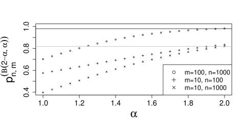
Figure 1.2.1. The probability $p^{(\Lambda)}_{n,m}$ of sharing the root between sample and subsample for $Beta(2-\alpha,\alpha)$-$n$-coalescents. Solid lines show the asymptotic probabilities $\lim_{n\to\infty}p^{(\delta_{0})}_{n,m}$ for Kingman’s $n$-coalescent for $m=10$ (in grey) and $m=100$ (in black).

Fig. 1.2.1 may raise the question whether Kingman’s $n$-coalescent is the $\Xi$-$n$-coalescent that has maximum $p_{n,m}^{(\Xi)}$. This is not true, for instance $\Xi$-$n$-coalescents that are essentially star-shaped, i.e. merge all individuals at the first merger with high probability, have a higher $p_{n,m}^{(\Xi)}$ if the probability for being star-shaped is high enough.

Due to the exchangeability of the $\Xi$-$n$-coalescent, $p^{(\Xi)}_{n,m}$ can alternatively be expressed in terms of the block sizes of the exchangeable partition of the $\Xi$-$n$-coalescent shortly before absorption.

Proposition 1.2.1.

[15, Props. 2 and 5] For any $\Xi$-$n$-coalescent,

(1.2.2) $$p^{(\Xi)}_{n,m}=1-E\Big{(}\sum_{i\in\mathbb{N}}\prod_{k=0}^{m-1}\frac{B^{(n)}_{[i]}-k}{n-k}\Big{)}>0,$$

where $B^{(n)}_{[1]},B^{(n)}_{[2]},\ldots$ are the sizes of the blocks of $\Pi^{(n)}$ merged at absorption, ordered by size from largest to smallest (filled up by empty blocks). The limit $p_{m}^{(\Xi)}:=\lim_{n\to\infty}p^{(\Xi)}_{(n,m)}$ exists and is greater than $0$ if and only if the $\Xi$-coalescent does not stay infinite. If the $\Xi$-coalescent comes down from infinity, we have

(1.2.3) $$p^{(\Xi)}_{n,m}\to 1-E\Big{(}\sum_{i\in\mathbb{N}}P_{[i]}^{m}\Big{)}=1-E(X^{m-1})=1-\frac{E(Y^{m})}{E(Y)}>0$$

for fixed $m$ and $n\to\infty$, where $P_{[i]}:=\lim_{n\to\infty}B^{(n)}_{[i]}/n$ is the asymptotic frequency of the $i$-th largest block merged at absorption, $X$ is the asymptotic frequency of a size-biased pick and $Y$ is the asymptotic frequency of a block picked uniformly at random from the blocks merging at absorption.

• This is a condensed version of the proof, focusing on the ideas and omitting technicalities.

  To see Eq. (1.2.2), first observe that $1-p^{(\Lambda)}_{(n,m)}$, the probability that the root is not shared, means that all individuals of $[m]$ have merged before the last merger. Thus, we need to have $[m]\subseteq B^{(n)}_{[i]}$ for some block of the partition merged at absorption. Given $B^{(n)}_{[1]},\ldots,B^{(n)}_{[n]}$, the probability of $[m]\subseteq(B^{(n)}_{[i]}$ is $\sum_{i=1}^{n}\prod_{\ell=0}^{m-1}$ $\big{(}B^{(n)}_{[i]}-\ell\big{)}/(n-\ell)$ for an $i\in[n]$ due to exchangeability.

  This allows us to consider $p_{m}^{(\Lambda)}:=\lim_{n\to\infty}p^{(\Lambda)}_{(n,m)}$ for fixed $m$. From the Poisson construction, one sees that adding more individuals can only add branches and nodes to the tree. Thus $p^{(\Lambda)}_{(n,m)}$ is monotonic in $n$ for $m$ fixed. When is the thus existing limit $p_{m}^{(\Xi)}=0$? If the $\Xi$-coalescent stays infinite, the waiting time for absorption, the height of the genealogy, diverges almost surely for $n\to\infty$. Thus, the root cannot be shared almost surely, so $p_{m}^{(\Xi)}=0$. Consider now the case that the coalescent does not stay infinite. As discussed above, this also means that the heights of the $\Xi$-$n$-coalescents equal the height of the $\Xi$-coalescent for $n$ large enough. Exchangeability (and elementary, yet technical arguments) ensures that the asymptotic frequencies of the blocks participating in the last merger exist. There are at least two blocks, no block has frequency 1, and again exchangeability ensures that with positive probability, $[m]$ is not a subset of a single block. This shows $p^{(\Xi)}_{m}>0$ if the coalescent does not stay infinite. The convergence in Eq. (1.2.3) follows directly due to the link between block sizes and asymptotic frequencies, while the characterisations using the size-biased and uniform picks are just standard characterisations of asymptotic frequencies in exchangeable partitions on $\mathbb{N}$. ∎

If one knows the moments of the asymptotic frequencies of the blocks of $\Pi^{(\Xi)}$ participating in the last merger, Eq. (1.2.3) would give an explicit formula for $p_{m}^{(\Xi)}$. For Beta-coalescents that come down from infinity, i.e. $1<\alpha<2$, there is an explicit characterisation of asymptotic frequencies, conditioned on the event that the Beta-coalescent is in a state with $k$ blocks, $k\in\mathbb{N}$. In this case, the asymptotic frequencies can be expressed in terms of Slack’s distribution, see [3, Thm. 1.2]. Since the distribution of the number of blocks $K$ participating in the last merger of this class of coalescents is also known, see [26], we can represent $p^{(\Xi)}_{m}$ as

(1.2.4) $$p^{(Beta(2-\alpha,\alpha))}_{m}=1-\sum_{k\in\mathbb{N}}k\frac{E\left(\frac{Y_{1}^{m}}{(Y_{1}+\ldots+Y_{k})^{\alpha+m-1}}\right)}{E\left((Y_{1}+\ldots+Y_{k})^{1-\alpha}\right)}P(K=k),$$

where $K$ has generating function $E(u^{K})=\alpha u\int_{0}^{1}(1-x^{1-\alpha})^{-1}((1-ux)^{\alpha-1}-1)\hskip 0.5pt\mathrm{d}\hskip 0.5ptx$ for $u\in[0,1]$ and $(Y_{i})_{i\in\mathbb{N}}$ are i.i.d. and have Slack’s distribution with Laplace transform $E\left(e^{-\lambda Y_{1}}\right)=1-(1+\lambda^{1-\alpha})^{-1/(\alpha-1)}$.

For $\alpha=1$, so for the Bolthausen–Sznitman ($n$-)coalescent, a more explicit representation can be derived from the connection to the uniform random permutation, aka the Chinese restaurant process.

Proposition 1.2.2.

[15, Prop. 4] Let $B_{1},\ldots,B_{n-1}$ be independent Bernoulli random variables with $P(B_{i}=1)=i^{-1}$. For $2\leqslant m<n$,

(1.2.5) $$p_{n,m}^{(Beta(1,1))}=E\left(\frac{B_{1}+\ldots+B_{m-1}}{B_{1}+\ldots+B_{n-1}}\right).$$

Moreover,

$$\log(n)p_{n,m}^{(Beta(1,1))}\to\sum^{m-1}_{i=1}i^{-1}\text{ for }n\to\infty\text{ and }m\text{ fixed.}$$

• The last merger of the Bolthausen–Sznitman $n$-coalescent has to feature one block including the individual 1. As described in the first section, the connection to the random recursive tree allows us to see the individuals subsequently merged to the block including 1 as adding the cycles of a uniform random permutation of $\{2,\ldots,n\}$ in random order. Since $1\in[m]$, the root is shared between subsample and sample if and only if the cycle added at the last merger also includes at least one $j\in[m]$. Using e.g. the Chinese restaurant process construction of the uniform random permutation, one sees that there are $\sum_{i=1}^{n-1}B_{i}$ cycles in the random permutation, from which $\sum_{i=1}^{m-1}B_{i}$ contain $j\in[m]$. This shows Eq. (1.2.5) and standard arguments establish its limit for $n\to\infty$. ∎

So what do these results imply for real populations? The main message is indeed Figure 1.2.1: Multiple merger genealogies, unless essentially star-shaped, will have a (often much) higher chance that enlargening collections of individuals uncovers new ancestral variation that then can be used for breeding. Adding population size changes of order $N$ only changes the distribution of branch lengths but not the tree topology (see Sect. 1.1) for all $\Lambda$-$n$-coalescents, so this holds true if we consider e.g. exponentially growing populations. However, if we are concerned about the actual shared genealogy, the picture changes somewhat. Using simulations, we assessed the fraction of internal branch length of the genealogy of $[n]$ that is already covered by the genealogy of $[m]$, see [15, Fig. 3-6]. On average, for Kingman’s $n$-coalescent a larger fraction of internal branches is covered by the subsample’s genealogy than for Beta-$n$-coalescents, while this is reversed for Kingman’s $n$-coalescent with strong exponential growth. Additionally, the coverage is much more variable for Beta-coalescents. Nevertheless, at least for small to medium growth rates, the benefit of larger samples in terms of added ancestral variation is stronger for multiple-merger genealogies. The results highlight that inferring the correct genealogy model can be relevant for real-life decisions concerning the population at hand.

One more technical, yet in my opinion important point should be discussed here. While we can characterise the limit behaviour of $p^{(\Xi)}_{n,m}$ for $n\to\infty$, this may not be of too much relevance for the practical application. This is not so much due to having finite sample sizes, but it is already questionable whether for $n$ large, the coalescent approximation still resembles the genealogy in the Cannings model, see e.g. [5] for addressing this issue for Kingman’s $n$-coalesent. However, due to the monotonicity of $p^{(\Xi)}_{n,m}$ for $m$ fixed and $n$ increasing, the limit results always give a lower bound for the probability of sharing the root between sample and subsample.

The results described in this section show that adding individuals for $\Lambda$- and $\Xi$-$n$-coalescent will usually have the effect that the genealogical tree is enlarged by a higher factor (increased height, but also increased internal branch length) than for Kingman’s $n$-coalescent. This may point to a conjecture for multiple-merger coalescents about the question posed by Felsenstein in [17]: “Do we need more sites, more sequences, or more loci?” if it comes to population genetic inference. While for Kingman’s $n$-coalescent, sample size is less important, our results indicate that this importance is elevated for multiple-merger $n$-coalescents.

1.3. Model selection between $n$-coalescents

During the two phases of the SPP 1590, much progress has been made on inference methods for deciding whether multiple merger genealogies explain the genetic diversity of a sample better than bifurcating genealogy models based on Kingman’s $n$-coalescent, both inside and outside of the SPP. For the former, see also the chapter by Birkner and Blath [6]. More formally, one is interested in performing model selection between two or more sets of $n$-coalescent models, each endowed with a range of mutation rates, based on the values of one or multiple statistics for measuring genetic diversity. Many methods focus on the site frequency spectrum $(\xi^{(n)}_{1},\ldots,\xi^{(n)}_{n-1})$ as inference statistics, where $\xi_{i}^{(n)}$ is the number of mutations that are inherited by exactly $i$ individuals in the sample, i.e. that have mutation allele count $i$, see e.g. [14, 37, 38, 40]. However, genetic data contains more information than the site frequency spectrum (SFS) and this surplus information can also be used to perform model selection, see e.g. [33] or [51]. A reliable method to use multiple statistics for model selection is Approximate Bayesian Computation (ABC). ABC uses a computational version of a Bayes approach, see e.g. [60] for an introduction. Consider we want to perform model selection between two models with equal a priori probability for each model. Data is represented by summary statistics. In the simplest ABC approach (rejection scheme), statistics are simulated $N\gg 1$ times with model parameters drawn from each model’s prior distribution (so $2N$ sets of summary statistics are produced). Then the posterior odds ratio between models is approximated by the ratio of the numbers of simulations from each model that are equal/very close to the observed value of the statistics (the quality of approximation depends e.g. on the sufficiency of the statistics used). See [39] for a recent review of more sophisticated approaches.

In [33], a variety of standard population genetic statistics were used in an ABC approach for model selection between Beta-$n$-coalescents and Kingman’s $n$-coalescent, both with exponential growth on the coalescent time scale. The SFS was further summarised by using its sum, the total number of observed mutations as well as the $(0.1,0.3,0.5,0.7,$ $0.9)$-quantiles of the mutation allele counts (this set of quantiles will be denoted by $AF$). Additionally, the authors used the same range of quantiles of the Hamming distances between all pairs (set of statistics denoted by $Ham$), of the squared correlation $r^{2}$ between the frequencies in the sample for each pair of mutations and, for a reconstruction of the genealogical tree by a standard phylogenetic methods (neighbor-joining), of the set of all branch lengths in the reconstructed tree (denoted by $Phy$). For distinguishing Beta-$n$-coalescents from Kingman’s $n$-coalescent, both also accounting for exponential growth on the coalescent time scale, they reported considerably lower error rates than earlier methods, e.g. [14], while also considering a slightly different setup. A crucial difference is that in [33], the range of mutation rates is identical for all $n$-coalescents considered. Since the distributions of height and total branch length differ strongly between different $n$-coalescent models, the number of observed mutations is also different. If statistics are used that are non-robust to the number of mutations on the genealogy, e.g. the number of segregating sites, this approach needs large ranges for the mutation rate to be able to reproduce these statistics as observed, which is not efficient for performing simulation-based inference approaches as ABC. If the parameter ranges are not large enough, model classes may produce the comparable numbers of mutations only with low probability or not at all, thus likely being discarded as the true model class. Thus, another approach (used in the other inference approaches mentioned) is to use mutation rates $\theta$ that produce a number of mutations in the range of the number $s$ of mutations observed in the data, e.g. by setting $\theta=\frac{2s}{E_{coal}(L_{n})}$ for each specific member $coal$ of a model class’s $n$-coalescents, which is the generalised form of Watterson’s estimator for $\theta$. Here, $L_{n}$ denotes the sum of the lengths of all branches of the coalescent tree. With Siri-Jégousse, I analyse which statistics considered by [33] are actually best to distinguish between different model classes featuring Kingman’s $n$-coalescent with exponential growth and several classes of $\Xi$-$n$-coalescents, including ones with exponential growth [21]. For this, we use the ABC approach for model selection based on random forests from [50] (random forests are a widely used machine learning approach introduced in [11]). Since it is an approximate Bayesian method, we need to specify prior distributions on both the coalescent classes and their mutation ranges. However, the approach from [50] differs drastically from the ABC approach presented above. In a nutshell, the method simulates a set of summary statistics $S_{1},S_{2},\ldots$ from each model class under its prior distribution, then takes bootstrap samples of these simulations. From each bootstrap sample, a decision tree is built, whose nodes have the form $S_{i}>t$ or $S_{i}<t$ for some $t\in\mathbb{R}$. For each node, the statistic that distinguishes best between model classes (normally measured by the Gini index, we use a slightly different measure), from a randomly drawn subset of statistics, is chosen as decider $S_{i}$. Nodes are added until the tree divides the bootstrap sample perfectly into sets of simulations from the same model class. The observed data is then sorted into a model class according to the decision tree for each bootstrap sample (so for the complete random forest), and the model selection is then the majority class across the forest. In other words, instead of using that the true model should produce summary statistics closer to the observed ones than another model, as e.g. rejection-scheme ABC, ABC based on random forests trains a forest of decision trees based on the simulations for the model priors and lets them decide, which model matches the observed statistics.

We chose this method mainly since it does not increase its model selection error when including many and potentially uninformative statistics and it comes with a built-in measure for the ability of each statistic to distinguish hypotheses, the variable importance. The variable importance of $S_{i}$ measures the average decline in misclassification over all nodes of the random forest where $S_{i}$ was picked as decider. To assess the misclassification errors, the ABC method uses the out-of-bag error. For this, one takes the fraction of trees in the random forest for each simulation sim that were built without sim and that sorted sim into a wrong model class (and then averages over all simulations).

As summary statistics, we use the statistics as in [33], but we add several more statistics, for instance nucleotide diversity $\pi$, the mean of the Hamming distances between all pairs of sampled individuals. We also add a new statistic. For each $i\in[n]$, $O_{n}(i)$ is the number of individuals including $i$ that share all non-private mutations of $i$ (a mutation is private if it is only found in one sampled individual). This correponds to the smallest allele count $>1$ of all mutations that affect individual $i$. See Figure 1.3.1 for an example. We consider the $(0.1,0.3,0.5,0.7,0.9)$-quantiles of $(O_{n}(i))_{i\in[n]}$ as well as the mean, standard deviation and harmonic mean as statistics, this set of statistics is denoted by $O$.

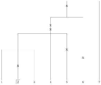
Figure 1.3.1. Genealogical tree, mutations marked by x. Individual 2 is affected by 4 mutations with allele counts 1,5,5,6. All non-private mutations are shared by individuals $[5]$. The observable minimal clade size of 2 is $O_{n}(2)=5$.

Our first result is that, not very surprisingly, including more statistics decreases the out-of-bag error meaningfully across a range of different sets of $n$-coalescents. See Table 1.3.1 for a comparison between model classes of Beta-$100$-coalescents (class Beta) for $\alpha\in[1,2)$ and Kingman’s $n$-coalescent with exponential growth (class Growth) and growth rate in $\rho\in[0,1000]$. We chose a uniform prior on $\alpha$, but (essentially) a $\log$ uniform prior on the growth rate, with an atom at $0$, to put a higher prior weight on low, more realistic growth rates (however, some real data sets of fungal or bacterial pathogens do fit relatively well to models with growth rates of 500 or more). The mutation rate $\theta$ was chosen for each model in any model class so that it produces, on average, a number of mutations $s\in\{15,20,30,40,60,75\}$, i.e. we draw $s$ from this set according to a (uniform) prior distribution and then set $\theta$ to the generalised Watterson estimate. We performed 175,000 simulations per model class. From these, we conducted the described ABC analysis. We perform the exact same analysis a second time, including new simulations with parameters from a new (and independent) draw from the prior distributions.

Set of statistics	Misclassification for Beta	Misclassification for Growth
$AF$, $S$,$\pi$	0.333 (0.330)	0.246 (0.246)
$AF$, $S$,$\pi$,$O$	0.246 (0.242)	0.205 (0.209)
$AF$, $S$,$\pi$,$Ham$	0.277 (0.274)	0.222 (0.227)
$AF$, $S$,$\pi$,$Phy$	0.317 (0.320)	0.247 (0.244)
$AF$, $S$,$\pi$,$r^{2}$	0.298 (0.290)	0.228 (0.235)
$AF$, $S$,$\pi$,$O$,$Ham$	0.241 (0.240)	0.203 (0.205)
FULL - $O$	0.269 (0.271)	0.217 (0.215)
FULL - $(AF,S,\pi)$	0.242 (0.240)	0.208 (0.210)
FULL	0.243 (0.240)	0.200 (0.204)

Table 1.3.1. Misclassification errors (out-of-bag errors) of the random forest ABC model comparison (5,000 trees) with different sets of summary statistics. In parentheses: results for rerun of analysis. FULL: $AF$,$S$,$\pi$,$O$,$Ham$,$Phy$,$r^{2}$

A more interesting take-away from our analysis is that adding statistics based on the minimal observable clade sizes $O$ to the set based on the allele counts $AF$, $S$, $\pi$ leads to considerably decreased error rates, which are only marginally reduced by further additions of statistics. The results are essentially unchanged if the full site frequency spectrum is used instead of $AF$. For the model selection using all considered statistics, the variable importance was highest for the harmonic mean of the minimal observable clade sizes. A potential explanation why the harmonic mean of $(O_{n}(i))_{i\in[n]}$ is a meaningful statistic for such model selections can be found in [21, p. 31-32] and has to do with the connection of $O_{n}(i)$ with the minimal clade size of $i$. These findings remain true for other model selection problems, e.g. if one changes the multiple merger genealogy model to a Dirac or Beta-$\Xi$-$n$-coalescent. The results presented here indicate that focusing on the site frequency spectrum for model selection between multiple merger and binary $n$-coalescents can be a suboptimal choice and that combining the information with further statistics as also done in [51] is advisable. A similar effect was observed for model selection between different scenarios of population size changes for bifurcating genealogies, see [31]. Due to the recent advance of full-data methods for such related inference problems, notably [48], where past population sizes are inferred based on a Kingman’s $n$-coalescent with fluctuating population sizes (essentially inferring the function $\nu$ from (1.1.1)) by an efficient representation of the full data, a revisit of full-likelihood methods may also be a viable alternative.

Where is this surplus of information for model selection really critical? For species with large enough genomes featuring many chromosomes and/or linkage blocks, the two studies [37] and [38] suggest that the information within the SFS is already enough to reliably distinguish between model classes over a range of different genealogy models (see the chapter of Birkner and Blath [6] in this volume). However, for e.g. bacteria with low recombination rates, where the entire genome can be essentially seen as one linkage block, this will not work as well. Here, pooling of more information than the SFS/AF clearly helps with distinguishing between model classes. An example of such bacteria is Mycobacterium tuberculosis, the bacterial agent of human tuberculosis, which is haploid and propagating clonally. Genealogies from M. tuberculosis outbreaks are usually modelled as Kingman’s $n$-coalescent with exponential growth. However, the bacteria have to evolve quickly due to a high selection pressure, which could lead to a Bolthausen–Sznitman $n$-coalescent as the suitable genealogy model. Moreover, real data shows some patients that are super-spreaders, i.e. infecting very many other patients, which could be modelled as a multiple-merger genealogy. With Menardo and Gagneux, I investigated in [41] whether indeed classes of $\Lambda$-$n$-coalescents fit better to the data than Kingman’s $n$-coalescent with exponential growth. We considered 11 publicly available data sets and performed model selection using the ABC approach described above. Our results show that 8 of 11 data sets actually fit better to multiple merger genealogies (10 of 11 if one allows for $\Lambda$-$n$-coalescents with exponential growth) and that these produce patterns of genetic diversity compatible with the observed data.

1.4. Partition blocks and minimal observable clades

Seeing that the minimal observable clade sizes are a reasonable addition to the arsenal of population genetic statistics, Siri-Jégousse and I also investigated their mathematical properties [22]. In the following, the key findings are presented. Looking back at Figure 1.3.1, the minimal observable clade of individual $i$ can be represented as the block including $i$ of the $\Xi$-$n$-coalescent at the time of the first mutation affecting $i$ that is not on the branch connecting leaf $i$ to the rest of the tree, i.e. on the external branch of $i$. Due to exchangeability, the distribution of the size of the minimal observable clade is identical for all $i\in[n]$, so in the following we fix $i=1$ and omit the $i$ for ease of notation. Let $O_{n}$ be the size of the minimal observable clade of 1 and $E_{n}$ the length of the external branch of 1. Since mutations are modelled by a homogeneous Poisson point process, independent of the $n$-coalescent, on the branches of the coalescent tree with rate $\frac{\theta}{2}$, the waiting time for the first non-private mutation on the path of leaf 1 to the root of the tree is $E_{n}+T_{n}$, where $T_{n}$ is a exponentially distributed with parameter $\frac{\theta}{2}$ independent of $E_{n}$ and of the coalescent. If $E_{n}+T_{n}$ exceeds the height of the $n$-coalescent tree, there is no non-private mutation of $i$ and thus $O_{n}=n$. Recall that $B^{(n)}_{1}(t)$ denotes the size of the block including 1 in the partition $\Pi^{(n)}_{t}$ induced by the $\Xi$-$n$-coalescent. Then, we can express

(1.4.1) $$O_{n}=B^{(n)}_{1}(E_{n}+T_{n}).$$

Based on this equation, we considered $O_{n}$ for $\Lambda$-$n$-coalescents. For finite $n$, all moments $E(O_{n}^{j})$, $j\in\mathbb{N}$, can again be computed recursively, see [22, Thm. 4.1]. Since the recursion for fixed $n$ is rather involved, yet relatively straightforward, let us focus on the asymptotics of $O_{n}$ for $n\to\infty$. Generally, for any $\Xi$-$n$-coalescent, $E_{n}$ decreases in $n$ and $E_{n}\stackrel{{\scriptstyle d}}{{\to}}Exp(\mu_{-1})$ for $n\to\infty$, where $\mu_{-1}=\int_{\Delta}\sum_{i=1}^{\infty}x_{i}\frac{\Xi(\hskip 0.5pt\mathrm{d}\hskip 0.5ptx)}{(x,x)}$. Thus, for $\Lambda$-$n$-coalescents without dust, $\mu_{-1}=\infty$ and $E_{n}\to 0$ almost surely. In this case, $O_{n}$ is asymptotically $B^{(n)}(T^{\prime})$, where $T^{\prime}\stackrel{{\scriptstyle d}}{{=}}Exp(\frac{\theta}{2})$, since this is the time until the first mutation in the coalescent tree on its path from leaf to root (which does not change with $n$, since the $n$-coalescents are nested, branches are added if $n$ grows). $T^{\prime}$ is independent from all $\Lambda$-$n$-coalescents. Kingman’s correspondence ensures that the asymptotic frequency $\lim_{n\to\infty}B^{(n)}_{1}(T^{\prime})/n=f_{1}(T^{\prime})$ exists almost surely, where $f_{1}(t)$ is the asymptotic frequency of the block including 1 at time $t$. This ensures $n^{-1}O_{n}\to f_{1}(T^{\prime})$ almost surely. When we additionally plug in the representation of the moments of $f_{1}(t)$ which follows from [49, Eq. (50) + Prop. 29], we can fully characterise the distribution of $f_{1}(T^{\prime})$ by its moments

(1.4.2) $$E\big{[}\big{(}f_{1}(T^{\prime})\big{)}^{k}\,\big{]}=1-\sum_{r=2}^{k+1}a_{k+1,r}\frac{\frac{\theta}{2}}{\lambda_{r}+\frac{\theta}{2}},$$

where $\lambda_{r}$ is the total rate of the $\Lambda$-coalescent in a state with $r$ blocks and $a_{k,r}$ is a rational function of $\lambda_{2},\ldots,\lambda_{k}$, defined as in [49, Prop. 29]. For the Bolthausen–Sznitman-$n$-coalescent ($\Lambda=Beta(1,1)$), we can show that the distribution of $f_{1}(T^{\prime})$ is a Beta distribution. For any $\Lambda$-$n$-coalescent, $f_{1}$ is a pure jump process and for $\Lambda=Beta(1,1)$, the countably many jumps are happening at i.i.d. $Exp(1)$ distributed times and their heights $(J_{i})_{i\in\mathbb{N}}$ are governed by a Poisson–Dirichlet distribution with parameters $(0,1)$, see [49, Cor. 16, Prop. 30]. Thus, each jump contributes to $f_{1}(T^{\prime})$ if its jump time is smaller than $T^{\prime}$, which happens with probability $\left(1+\frac{\theta}{2}\right)^{-1}$. This shows that $f_{1}(T^{\prime})\stackrel{{\scriptstyle d}}{{=}}\sum_{i\in\mathbb{N}}B_{i}J_{i}$, where $(B_{i})_{i\in\mathbb{N}}$ are i.i.d. Bernoulli random variables with success probability $\left(1+\frac{\theta}{2}\right)^{-1}$, and this sum has a $Beta\big{(}\left(1+\frac{\theta}{2}\right)^{-1},\frac{\theta}{2}\left(1+\frac{\theta}{2}\right)^{-1}\big{)}$-distribution, which can be seen from the construction of the Poisson–Dirichlet distribution via a Poisson point process, as e.g. in [2, Sect. 4.11].

If the $\Lambda$-$n$-coalescent has dust, the asymptotic decoupling of $f_{1}$ and the time until the first mutation on the path from individual 1 to the root that is not on the external branch breaks down. However, if a $\Xi$-coalescent has dust and stays infinite, the block frequency $f_{1}$ can be characterised from jump to jump, which I showed in joint work with Möhle.

Proposition 1.4.1.

[20, Thm. 1] In any $\Xi$-coalescent with dust that stays infinite, $(f_{1}(t))_{t\geqslant 0}$ is an increasing pure jump process with càdlàg paths, $f_{1}(0)=0$ and $\lim_{t\to\infty}f_{1}(t)=1$, but $f_{1}(t)<1$ for $t>0$ almost surely. The waiting times between the almost surely infinitely many jumps are distributed as independent ${\rm Exp}(\mu_{-1})$ random variables. Its jump chain $(f_{1}[k])_{k\in\mathbb{N}}$ can be expressed via stick-breaking

(1.4.3) $$f_{1}[k]=\sum_{i=1}^{k}X_{i}\prod_{j=1}^{i-1}(1-X_{j}),$$

where the $(X_{j})_{j\in\mathbb{N}}$ are pairwise uncorrelated, $X_{j}>0$ almost surely and $E(X_{j})=\gamma:=\frac{\Xi(\Delta)}{\mu_{-1}}$ for all $j\in\mathbb{N}$. Moreover, $E(f_{1}[k])=1-(1-\gamma)^{k}$. In general, the $(X_{j})_{j\in\mathbb{N}}$ are neither independent nor identically distributed.

Proof.

Here, only a sketch of the proof is excerpted from [20], focusing on the waiting times between jumps and their expected height. The expected height is given in terms of the mass added to the asymptotic frequency $f_{1}(t-)$ if the $k$th jump is at time $t$, and thus has the form $X_{k}(1-f_{1}(t-))$. First, observe that if the $\Xi$-coalescent has dust, $\Xi(\{(0,0,\ldots)\})=0$, which means that any $\Xi$-$n$-coalescent can be constructed by colouring according to a Poisson point process on $[0,\infty)\times\Delta$ with intensity $\hskip 0.5pt\mathrm{d}\hskip 0.5ptt\otimes\frac{\Xi(\hskip 0.5pt\mathrm{d}\hskip 0.5ptx)}{(x,x)}$ without having to add additional mergers of two blocks. Recall the Poisson point construction of a $\Xi$-$n$-coalescent from Section LABEL:FF-sect:intro, especially how mergers are determined by throwing independent balls on a ‘paintbox’ $x\in\Delta$ and merging blocks whose balls have the same colour (landed in the same compartment of $x$). As also mentioned in the first section, if the $\Xi$-coalescent has dust, there are almost surely only finitely many Poisson points $(t,x)$ where the block containing $i$ is coloured. More precisely, each Poisson point is affecting the block containing 1 with probability $\sum_{i\in\mathbb{N}}x_{i}$. Dividing the points of the original Poisson point into those that colour the block including 1 leads to a marked Poisson process, so the Poisson points affecting the block including 1 form again a Poisson point process on $[0,\infty)\times\Delta$ with intensity measure $\nu_{1}=\hskip 0.5pt\mathrm{d}\hskip 0.5ptt\otimes\sum_{i\in\mathbb{N}}x_{i}\frac{\Xi(\hskip 0.5pt\mathrm{d}\hskip 0.5ptx)}{(x,x)}$. Since the coalescent stays infinite, every such point, due to the strong law of large numbers for exchangeable random variables, will colour infinitely many blocks with this colour. For $f_{1}$, we can thus describe its jump by just merging the blocks of the $\Xi$-coalescent according to the colouring at each Poisson point affecting the block including 1 (though the Poisson points not affecting 1 do change the frequencies of these blocks). The probability for not having a Poisson point affecting 1 with time component $t$ in any interval of length $t_{0}$ is given by $\exp\big{(}-\nu_{1}([t^{\prime},t^{\prime}+t_{0})\times\Delta)\big{)}=\exp(-t_{0}\mu_{-1})$, which verifies the distribution of the waiting times. At such a Poisson point $(t,x)$, any other block merges with the block including 1 if it has the same colour $i$ (which the block including 1 picks with probability $\frac{x_{i}}{\sum_{i\in\mathbb{N}}x_{i}}$), so with probability $x_{i}$, regardless of its frequency. Each $x$ is drawn from the probability distribution $(\mu_{-1})^{-1}\sum_{i\in\mathbb{N}}x_{i}\frac{\Xi(\hskip 0.5pt\mathrm{d}\hskip 0.5ptx)}{(x,x)}$. All blocks not containing 1 have total frequency $1-f_{1}(t-)$ when potentially merging at $(t,x)$, so the average fraction of mass from $1-f_{1}(t-)$ added to $f_{1}(t-)$ is

$$E(X_{k})=\frac{1}{\mu_{-1}}\int_{\Delta}\sum_{i\in\mathbb{N}}\frac{x_{i}^{2}}{\sum_{k\in\mathbb{N}}x_{k}}\sum_{\ell\in\mathbb{N}}x_{\ell}\frac{\Xi(\hskip 0.5pt\mathrm{d}\hskip 0.5ptx)}{(x,x)}=\frac{\Xi(\Delta)}{\mu_{-1}}.$$

∎

This result can now be applied to address the asymptotics of $O_{n}$ for $\Lambda$-$n$-coalescents with dust if the coalescent stays infinite, i.e. $\Lambda(\{1\})=0$. Let $T_{1},T_{2},\ldots$ be the i.i.d. jump times of $f_{1}$. Clearly, $E_{n}=T_{1}$ for $n$ large enough. Similarly as in the case without dust, we can then see that there is a time $T^{\prime}$, not dependent on $n$, when the first mutation after time $T_{1}$ appears on the path from leaf 1 to the root of the $\Xi$-$n$-coalescent, and this, for $n$ large enough, will fall in between two jumps of $f_{1}$, say $K$ and $K+1$. Thus, Proposition 1.4.1 ensures that $\lim_{n\to\infty}n^{-1}O_{n}=f_{1}[K]$ exists almost surely. $K$ is geometrically distributed on $\mathbb{N}$ with success probability $\frac{\mu_{-1}}{\mu_{-1}+\frac{\theta}{2}}$, since the exponential distribution is memoryless and the probability that one exponential random variable is smaller than another one independent of it is given by the exponential rate of the first divided by the sum of the rates. With Proposition 1.4.1, one can compute $E(f_{1}[K])=1-\frac{\theta}{2\mu_{-1}}\frac{a}{1-a}$ with $a=\left(1-\frac{\Lambda([0,1])}{\mu_{-1}}\right)\left(\frac{\frac{\theta}{2}}{\frac{\theta}{2}+\mu_{-1}}\right)$.

The process $(f_{1}(t))_{t\geqslant 0}$ has some interesting further properties. While it is Markovian when observed in the Bolthausen–Sznitman $n$-coalescent, see [49, Cor. 16], it is not in general. For instance, by further exploiting the Poisson construction, the following properties of $f_{1}$ for Dirac coalescents can be derived.

Proposition 1.4.2.

[20, essentially Prop. 2] Let $\Lambda=\delta_{p}$, $p\in[\frac{1}{2},1)$ or $p\in(0,\frac{1}{2})$ and transcendental, and $q:=1-p$. $f_{1}$ takes values in the set

$$\mathcal{M}_{p}:=\Big{\{}\sum_{i\in\mathbb{N}}b_{i}pq^{i-1}:b_{i}\in\{0,1\},\sum_{i\in\mathbb{N}}b_{i}<\infty\Big{\}}.$$

For $x=\sum_{i\in\mathbb{N}}b_{i}pq^{i-1}\in\mathcal{M}_{p}$, we have

$$P(f_{1}[1]=x)=pq^{j-1}\prod_{i\in J\setminus\{j\}}P(Y+i\in J)\prod_{i\in[j-1]\setminus J}P(Y+i\notin J)>0,$$

where $Y\stackrel{{\scriptstyle d}}{{=}}Geo(p)$, $J:=\{i\in\mathbb{N}\mid b_{i}=1\}$ and $j:=\max J$. The process $f_{1}$ is not Markovian whereas its jump chain $(f_{1}[k])_{k\in\mathbb{N}}$ is Markovian.

Under the condition for $p$ from the proposition, knowing that $f_{1}[1]=x$ allows to directly infer information about mergers at or before the time the minimal clade is formed: Each collision of a Dirac coalescent (on $\mathbb{N}$) merges a fraction of $p$ of all singleton blocks present (the ‘dust’), so each each block has asymptotic frequency from $\mathcal{M}_{p}$. The condition on $p$ ensures that $x\in\mathcal{M}_{p}$ has a unique representation in terms of the $b_{i}$’s. Moreover, the $b_{i}$’s encode at which Poisson point the minimal clade appears and which fraction of singletons merged at earlier Poisson points are merged to form the minimal clade. If one drops the condition on $p$, the distribution of $f_{1}[1]$ would become more involved, since one would have to trace back which combinations of $b_{i}$’s lead to the same $x$ and sum these.

References

- [1] E. Árnason and K. Halldórsdóttir, Nucleotide variation and balancing selection at the Ckma gene in Atlantic cod: Analysis with multiple merger coalescent models, PeerJ 3 (2014), e786.
- [2] R. Arratia, A.D. Barbour, and S. Tavaré, Logarithmic Combinatorial Structures: A Probabilistic Approach, EMS, Zürich, 2003.
- [3] J. Berestycki, N. Berestycki, and J. Schweinsberg, Small-time behavior of beta coalescents, Ann. Inst. Henri Poincaré Prob. Stat. 44 (2008), 214–238.
- [4] J. Berestycki, N. Berestycki, and J. Schweinsberg, The genealogy of branching Brownian motion with absorption, Ann. Probab. 41 (2013), 527–618.
- [5] A. Bhaskar, A.G. Clark, and Y.S. Song, Distortion of genealogical properties when the sample is very large, PNAS 111 (2014), 2385–2390.
- [6] M. Birkner and J. Blath, Genealogies and inference for populations with highly skewed offspring distributions, this volume, arXiv:1912.07977.
- [7] M. Birkner, J. Blath, and B. Eldon, An ancestral recombination graph for diploid populations with skewed offspring distribution, Genetics 193 (2013), 255–290.
- [8] M. Birkner, H. Liu, and A. Sturm, Coalescent results for diploid exchangeable population models, Electron. J. Probab. 23 (2018), paper no. 49, 44 pp.
- [9] J. Blath, M.C. Cronjäger, B. Eldon, and M. Hammer, The site-frequency spectrum associated with -coalescents, Theor. Popul. Biol. 110 (2016), 36–50.
- [10] J. Blath and N. Kurt, Population genetic models of dormancy, this volume.
- [11] L. Breiman, Random forests, Machine Learning 45 (2001), 5–32.
- [12] É. Brunet and B. Derrida, Genealogies in simple models of evolution, J. Stat. Mech. (2013), P01006.
- [13] M.M. Desai, A.M. Walczak, and D.S. Fisher, Genetic diversity and the structure of genealogies in rapidly adapting populations, Genetics 193 (2013), 565–585.
- [14] B. Eldon, M. Birkner, J. Blath, and F. Freund, Can the site-frequency spectrum distinguish exponential population growth from multiple-merger coalescents?, Genetics 199 (2015), 841–856.
- [15] B. Eldon and F. Freund, Genealogical properties of subsamples in highly fecund populations, J. Stat. Phys. 172 (2018), 175–207.
- [16] B. Eldon and J. Wakeley, Coalescent processes when the distribution of offspring number among individuals is highly skewed, Genetics 172 (2006), 2621–2633.
- [17] J. Felsenstein, Accuracy of coalescent likelihood estimates: do we need more sites, more sequences, or more loci?, Mol. Biol. Evol. 23 (2006), 691–700
- [18] Food and Agriculture Organization of the United Nations, WIEWS — World information and early warning system on plant genetic resources for food and agriculture, http://www.fao.org/wiews/glossary/en/
- [19] F. Freund, Cannings models, populations size changes and multiple-merger coalescents, J. Math. Biol. 80 (2020), 1497–1521.
- [20] F. Freund and M. Möhle, On the size of the block of 1 for -coalescents with dust, Mod. Stoch. Th. Appl. 4 (2017), 407–425.
- [21] F. Freund and A. Siri-Jégousse, The impact of genetic diversity statistics on model selection between coalescents, to appear in Comput. Stat. Data Anal.; preprint, bioRxiv 679498.
- [22] F. Freund and A. Siri-Jégousse, The minimal observable clade size of exchangeable coalescents, to appear in Braz. J. Probab. Stat.; preprint, arXiv:1902.02155.
- [23] C. Goldschmidt and J.B. Martin, Random recursive trees and the Bolthausen-Sznitman coalescent, Electron. J. Probab. 10 (2005), 718–745.
- [24] R.C. Griffiths and S. Tavaré, Sampling theory for neutral alleles in a varying environment, Philos. Trans. Royal Soc. B 344 (1994), 403–410.
- [25] D. Hedgecock and A.I. Pudovkin, Sweepstakes reproductive success in highly fecund marine fish and shellfish: a review and commentary, Bull. Marine Sci. 87 (2011), 971–1002.
- [26] O. Hénard, The fixation line in the -coalescent, Ann. Appl. Prob. 25 (2015). 3007–3032.
- [27] P. Herriger and M. Möhle, Conditions for exchangeable coalescents to come down from infinity, ALEA 9 (2012), 637–665.
- [28] P. Hoscheit and O. Pybus, The multifurcating skyline plot, Virus Evolution 5 (2019), vez031.
- [29] T. Huillet and M. Möhle, On the extended Moran model and its relation to coalescents with multiple collisions, Theor. Popul. Biol. 87 (2013), 5–14.
- [30] K.K. Irwin, S. Laurent, S. Matuszewski, S. Vuilleumier, L. Ormond, H. Shim, C. Bank, and J.D. Jensen, On the importance of skewed offspring distributions and background selection in virus population genetics, Heredity 117 (2016), 393–399.
- [31] F. Jay, S. Boitard, and F. Austerlitz, An ABC method for whole-genome sequence data: inferring paleolithic and neolithic human expansions, Mol. Biol. Evol. 36 (2019), 1565–1579.
- [32] I. Kaj and S.M. Krone, The coalescent process in a population with stochastically varying size, J. Appl. Prob. 40 (2003), 33–48.
- [33] M. Kato, D.A. Vasco, R. Sugino, D. Narushima, and A. Krasnitz, Sweepstake evolution revealed by population-genetic analysis of copy-number alterations in single genomes of breast cancer. Royal Soc. Open Sci. 4 (2017), 20170011.
- [34] G. Kersting and A. Wakolbinger, Probabilistic aspects of -coalescents in equilibrium and in evolution, this volume, arXiv:2002.05250.
- [35] J.F.C. Kingman, On the genealogy of large populations, J. Appl. Prob. 19 (1982), 27–43.
- [36] J.F.C. Kingman, The coalescent, Stochastic Processes Appl. 13 (1982), 235–248.
- [37] J. Koskela, Multi-locus data distinguishes between population growth and multiple merger coalescents, Stat. Appl. Genet. Mol. Biol. 17 (2018).
- [38] J. Koskela and M. Wilke Berenguer, Robust model selection between population growth and multiple merger coalescents, Math. Biosci. 311 (2019), 1–12.
- [39] J. Lintusaari, M.U. Gutmann, R. Dutta, S. Kaski, and J. Corander, Fundamentals and recent developments in approximate Bayesian computation, Syst. Biol. 66 (2017), e66–e82.
- [40] S. Matuszewski, M.E. Hildebrandt, G. Achaz, and J.D. Jensen, Coalescent processes with skewed offspring distributions and non-equilibrium demography, Genetics 208 (2018), 323–338.
- [41] F. Menardo, S. Gagneux, and F. Freund, Multiple merger genealogies in outbreaks of Mycobacterium tuberculosis, to appear in Mol. Biol. Evol.; preprint, bioRxiv 885723.
- [42] M. Möhle, The coalescent in population models with time-inhomogeneous environment, Stochastic Processes Appl. 97 (2002), 199–227.
- [43] M. Möhle, Total variation distances and rates of convergence for ancestral coalescent processes in exchangeable population models, Adv. Appl. Prob. 32 (2000), 983–993.
- [44] M. Möhle and S. Sagitov, A classification of coalescent processes for haploid exchangeable population models, Ann. Prob. 29 (2001), 1547–1562.
- [45] R.A. Neher and O. Hallatschek, Genealogies of rapidly adapting populations, PNAS 110 (2013), 437–442.
- [46] H.-S. Niwa, K. Nashida, and T. Yanagimoto, Reproductive skew in Japanese sardine inferred from DNA sequences, ICES J. Marine Sci. 73 (2016), 2181–2189.
- [47] A. Nourmohammad, J. Otwinowski, M. Łuksza, T. Mora, and A.M. Walczak, Fierce selection and interference in B-cell repertoire response to chronic HIV-1. Mol. Biol. Evol. 36 (2019), 2184–2194.
- [48] J.A. Palacios, A. Veber, L. Cappello, Z. Wang, J. Wakeley, and S. Ramachandran, Bayesian estimation of population size changes by sampling Tajima’s trees, Genetics 213 (2019), 967–986.
- [49] J. Pitman, Coalescents with multiple collisions, Ann. Prob. 27 (1999), 1870–1902.
- [50] P. Pudlo, J.-M. Marin, A. Estoup, J.-M. Cornuet, M. Gautier, and C.P. Robert, Reliable ABC model choice via random forests, Bioinformatics 32 (2015), 859–866.
- [51] D.P. Rice, J. Novembre, and M.M. Desai, Distinguishing multiple-merger from Kingman coalescence using two-site frequency spectra, preprint, bioRxiv 461517.
- [52] C. Rödelsperger, R.A. Neher, A.M. Weller, G. Eberhardt, H. Witte, W.E. Mayer, C. Dieterich, and R.J. Sommer, Characterization of genetic diversity in the nematode Pristionchus pacificus from population-scale resequencing data, Genetics 196 (2014), 1153–1165.
- [53] I.W. Saunders, S. Tavaré, and G.A. Watterson, On the genealogy of nested subsamples from a haploid population, Adv. Appl. Probab. 16 (1984), 471–491.
- [54] J. Schweinsberg, Coalescents with simultaneous multiple collisions, Electron. J. Probab. 5 (2000), 1–50.
- [55] J. Schweinsberg, Coalescent processes obtained from supercritical Galton–Watson processes, Stochastic Processes Appl. 106 (2003), 107–139.
- [56] J. Schweinsberg, Rigorous results for a population model with selection ii: genealogy of the population, Electron. J. Probab. 22 (2017).
- [57] J.P. Spence, J.A. Kamm, and Y.S. Song, The site frequency spectrum for general coalescents, Genetics 202 (2016), 1549–1561.
- [58] M. Steinrücken, M. Birkner, and J. Blath, Analysis of DNA sequence variation within marine species using Beta-coalescents. Theor. Popul. Biol. 87 (2013), 15–24.
- [59] A. Sturm, Diploid populations and their genealogies, this volume.
- [60] M. Sunnåker, A.G. Busetto, E. Numminen, J. Corander, M. Foll, and C. Dessimoz, Approximate Bayesian computation, PLoS Comp. Biol. 9 (2013), e1002803.
- [61] A. Tellier and C. Lemaire, Coalescence 2.0: a multiple branching of recent theoretical developments and their applications, Mol. Ecol. 23 (2014), 2637–2652.