Atomic Permutationally Invariant Polynomials for Fitting Molecular Force Fields

Abstract

We introduce and explore an approach for constructing force fields for small molecules, which combines intuitive low body order empirical force field terms with the concepts of data driven statistical fits of recent machine learned potentials. We bring these two key ideas together to bridge the gap between established empirical force fields that have a high degree of transferability on the one hand, and the machine learned potentials that are systematically improvable and can converge to very high accuracy, on the other. Our framework extends the atomic Permutationally Invariant Polynomials (aPIP) developed for elemental materials in [Mach. Learn.: Sci. Technol. 2019 1 015004] to molecular systems. The body order decomposition allows us to keep the dimensionality of each term low, while the use of an iterative fitting scheme as well as regularisation procedures improve the extrapolation outside the training set. We investigate aPIP force fields with up to generalised 4-body terms, and examine the performance on a set of small organic molecules. We achieve a high level of accuracy when fitting individual molecules, comparable to those of the many-body machine learned force fields. Fitted to a combined training set of short linear alkanes, the accuracy of the aPIP force field still significantly exceeds what can be expected from classical empirical force fields, while retaining reasonable transferability to both configurations far from the training set and to new molecules.

I Introduction

Molecular mechanics (MM) with classical empirical force fields has been used to perform simulations of organic molecules for many decades Jorgensen and Tirado-Rives (1988); Weiner et al. (1984). One of the principle reasons why such force fields have been so successful is that the simplicity of their functional form results in both a low body order and relatively few fitting parameters. This allows the parameters to be fit using just a small amount of quantum mechanical (QM) or experimental data, and the problems associated with overfitting do not readily occur. The simple, chemically intuitive functional form makes the force fields highly transferable, giving reasonable results for molecules and conformations far away from those that were used to fit the parameters. Over time, improvements were made in the description of both the intermolecular interactions, particularly through the construction of polarizable models Ponder et al. (2010), and the intramolecular interactions, mainly with the development of Class II force fields Maple et al. (1994); Ewig et al. (2001); Sun et al. (2016) that introduced new couplings between bond and angle terms. However, despite these developments the accuracy of classical force fields remains limited by the restrictive functional forms, the very same that gave rise to their success. This is particularly noticable when having to make unavoidable trade-offs between the accuracy of different observables. Freeing up the functional form has been achieved for only low body orders (up to three-body) e.g. in the ChIMES force field Lindsey et al. (2017, 2019).

Over the past few years, a completely new direction emerged: the development of machine learning (ML) based potentials Behler and Parrinello (2007); Bartók et al. (2010) has led to a significant improvement in accuracy for small molecules Behler (2011a); Rupp et al. (2012); Bartók et al. (2013, 2013); Behler (2015); Manzhos et al. (2015); Behler (2016); Bartók et al. (2017); Smith et al. (2017); Chmiela et al. (2017, 2018); Veit et al. (2019). It has been demonstrated that these new ML models can perform molecular dynamics (MD) simulations in some cases and be transferred to some extent to molecules they have not been explicit fit to Smith et al. (2019). The long term goal of these developments is to obtain a general model having an accuracy comparable to accurate ab initio methods such as CCSD(T) Raghavachari et al. (1989), and a speed and transferability comparable to classical force fields. The various formalisms of the recent ML models represent, on the surface, a radical departure from that of empirical force fields. The aim of this paper is to bridge this formalism gap, and to seek answers to questions such as: what makes the ML models accurate, is it their high dimensionality (i.e. body order) or their flexible functional form? How much additional accuracy is gained by allowing a controlled increase in body order?

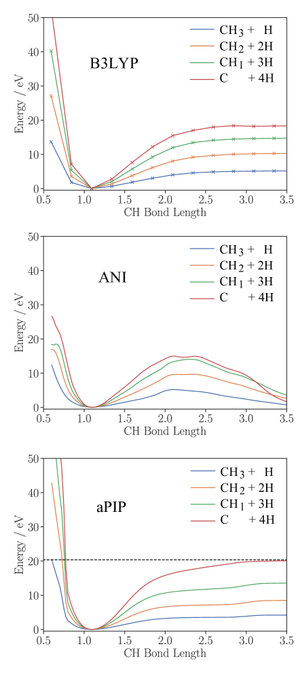
Figure 1: Removing some number of hydrogens from methane using DFT/B3LYP (top), ANI (middle) and aPIPs (bottom). Both ANI and the aPIP were fitted only to near equilibrium geometries (the aPIP shown here was fitted to a database of small linear alkanes, including distortions of bond lengths up to 0.3 Å).

Predating the recent surge of interest in machine learned force fields, there is a significant literature for accurate fitting of molecular potential energy surfaces (PES) Behler (2016); Deringer et al. (2019). One of the most prominent and systematic approaches is due to Bowman and Braams Braams and Bowman (2009); Huang et al. (2005); Xie et al. (2005); Qu and Bowman (2019); Nandi et al. (2019). Given a fixed molecular composition, a basis consisting of permutationally invariant polynomials (PIPs) of the interatomic distances is constructed and then used to approximate the PES by least squares fitting. Models using PIPs have very high accuracy, below 1 meV/molecule, and successfully reproduced the properties of a number of small molecules including $\mathrm{CH_{5}^{+}}$, $\mathrm{H_{2}O}_{2}$ and malonaldehyde Braams and Bowman (2009); Huang et al. (2005); Xie et al. (2005). They have also been used as building blocks in models of water such as MBpol by Paesani et al Babin et al. (2012, 2013, 2014); Medders et al. (2014), probably the most accurate water model to date.

The difficulty in extending the PIP formalism to larger molecules or larger clusters of small molecules is in the scaling of the computational cost with the number of atoms. The number of permutationally invariant polynomials that are used as the basis grows factorially, in fact we were unable to obtain basis functions for six atoms of the same kind with full permutation symmetry. One way out of this crushing scaling is to employ a so-called “fragmentation scheme” Qu and Bowman (2019), in which parts of the molecule are explicitly grouped into fragments, and permutations between the groups are excluded from the symmetries of the basis. However, the choice of the fragments, based on distances in the initial molecule template, is manual and therefore limited to molecules which can be clearly split into suitable fragments. Potentials for large cyclic molecules or flexible molecules cannot be produced with this method.

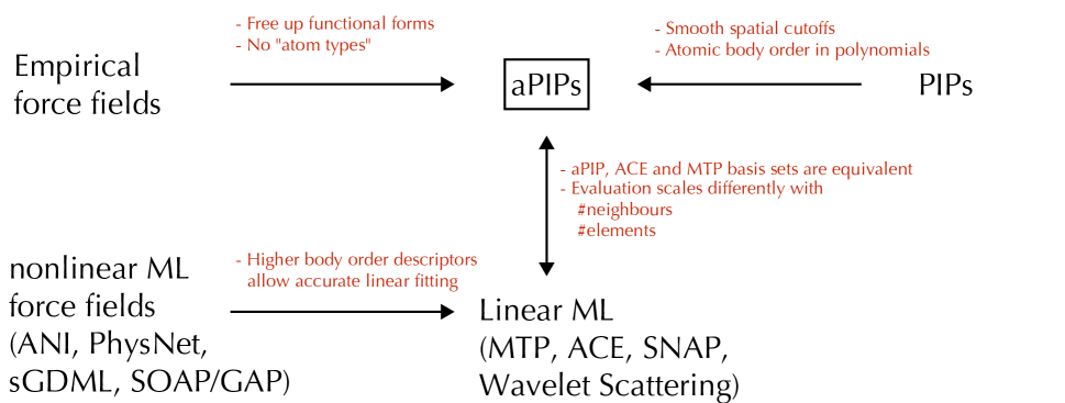
Figure 2: Top: Relationships between different force field schemes. Bottom: a graphical representation of the body order terms in empirical force fields and in the aPIP framework. The shading of the 3-,4- and 5-simplices emphasises that full dimensionality of the simplex is represented, and thus the $n=$ 3-, 4-, and 5-body terms are 3, 6 and 9 dimensional functions, respectively (given by $3n-6$). On the right, the cartoons represent (i) the PIP method of Bowman & Braams Braams and Bowman (2009) and sGDML Chmiela et al. (2019) that both describe a whole molecule always using its full dimensional representation, and (ii) atom-centered ML methods Smith et al. (2017); Bartók and Csányi (2015) that represent the complete environment of an atom up to a cutoff. All of these approaches are many-body and do not take advantage of the atomic body-ordered decomposition in the way empirical force fields and aPIPs do.

A little over a decade ago, a new approach to making potentials was devised, inspired by the developments in computer science. Instead of systematically expanding the potential energy function using an analytically defined basis set, or using carefully designed chemically intuitive descriptions of atomic interactions, the idea was to describe the entire local neighbourhood of an atom using a set of descriptors, and then use nonlinear regression techniques to fit a model with thousands of parameters to first principles data. First, Behler and Parrinello introduced atom-centered symmetry functions and used a feed-forward artificial neural networks Behler and Parrinello (2007); later, spherical harmonics were used in combination with Gaussian process (kernel) regression Bartók et al. (2010). These new approaches led to exquisitely accurate interatomic potentials for strongly bound materials Bartók et al. (2013); Behler (2011b); Bartók et al. (2017); Behler (2017); Bartók et al. (2018) and condensed phase molecular materials Bartók et al. (2013); Morawietz and Behler (2013); Gastegger et al. (2016); Nguyen et al. (2018); Veit et al. (2019). Although using neural networks to fit potentials was not itself new (e.g. see Refs. 43; 44) these aforementioned models had finite interaction range, resulting in linear scaling cost, which opened the door to simulations of large systems with unprecedented accuracy.

The field has since blossomed, with many novel approaches introduced Manzhos et al. (2015); Thompson et al. (2015); Shapeev (2016a); Kolb et al. (2016); Huang and von Lilienfeld (2017); Schutt et al. (2017); Yao et al. (2018); Unke and Meuwly (2019). Particularly notable is the ANI series of models for organic molecules Smith et al. (2017, 2018, 2019). For moderate sized molecules and small clusters very accurate custom made (non-transferable) models can be made using simply the interatomic distances as the set of descriptors and a Gaussian kernel Bartók et al. (2013, 2013); Chmiela et al. (2017, 2018); Cole et al. (2020). Along with these successes, however, due to the high dimensional nature of these fits, come the problems of extrapolation and transferability. All these ML models (both for materials and molecules) are guaranteed to be accurate only for configurations quite near their training set, and can become uncontrolled or even nonsensical far from there. The practice of making ML models has therefore largely focused on how to create suitable (and rather large) training sets, how to detect when the model goes “out of scope” etc. Such problems do not exist for the empirical force fields: although their accuracy is only moderate, and not systematically improvable, they never give catastrophically incorrect results. They behave much more reasonably in extrapolation, even without explicit fitting to such configurations, since chemical intuition is built in through the functional form and leads to much lower-dimensional objects to fit.

An illustration of such a problem is in Fig. 1, showing the ANI modelSmith et al. (2017) behaving unphysically as hydrogens are removed from a methane molecule. The reason is simple: neither such bond dissociations, nor isolated atoms were included in its fitting database; no doubt if they were, the results would look much better. We emphasise that this is no indictment of the ANI model in particular, and we expect all direct high dimensional fits to behave similarly, or worse.

In this work, we introduce a way of making force fields for molecules that has the transferability and reasonable extrapolation property, due to limited body order, of empirical force fields, and also the accuracy of the recent ML models, due to its systematic nature. The construction, which we call atomic permutationally invariant polynomials (aPIP), builds heavily on the PIP framework of Bowman and Braams, and generalises our earlier work for strongly bound materials Ref. 54. We show that the “best of both worlds” is possible: chemically sensible functions leading to smooth dissociation curves, as shown in Fig 1, without compromising on the convergence and ultimate accuracy of the fit. Before we introduce the construction of multi-element aPIPs in detail, it is helpful to note that they can be viewed in two ways.

When developing empirical force fields, adding terms to the functional form is a natural way to improve a potential’s accuracy, as was shown in the development of Class II force fields Maple et al. (1994); Sun et al. (2016); Ewig et al. (2001). These have additional cross-terms between the bond, angle and dihedral components and include higher degree terms Maple et al. (1994). This indeed improves the accuracy of the force field Tsai and Simpson (2003) but these additional higher body order terms introduce only very few new degrees of freedom. Manually adding such terms to the functional form becomes increasingly tedious and complex. The aPIP construction can be viewed as a general framework to implement this idea of systematically increasing to arbitrary body order, while allowing for the full dimensional freedom at each order. By increasing the degree of the polynomials, the functional form becomes increasingly complex as higher degree bond and angle terms, as well as all possible cross-terms between angles and bonds, are automatically included. By retaining the atom-wise body ordered description, the dimensionality of the representation is kept small, as is the case for empirical force fields. (In fact existing empirical force fields can all be represented as aPIPs.) This is the crucial way in which aPIPs differ from the regular PIPs of Bowman and Braams, and brings us to the second, complementary view of aPIPs. They can instead be viewed as a version of PIPs in which we limit the combinatorial explosion in the number of terms with system size by (i) explicitly limiting the body order of the potential, and (ii) using a smooth spatial cutoff. The latter can be seen as an automated way to implement the aforementioned “fragmentation” process, and also brings an atom centered view. In fact, it can be shown that in the limit of high body order, the aPIP basis is equivalent to the high dimensional ML approaches, and particularly closely linked to MTP Shapeev (2016a) and ACE Drautz (2019); Bachmayr et al. (2019). Figure 2 shows the conceptual relationships between many of the approaches mentioned in this section. The key advance with aPIPs is the ability to gradually and systematically increase the body order, describing each term in its full generality.

Two more short points are in order. Firstly, due to the smooth cutoff we introduce, discrete atom types, as used in empirical force fields, are no longer necessary, although could still be used if desired. Secondly, just as empirical force fields have separate short and long range interaction terms, so too can aPIPs. We focus in this paper on the short range intramolecular interactions. Any existing long range model, whether describing electrostatics of van der Waals dispersion, can be added if desired.

The construction of the aPIP potential is as follows. To start with, the total energy is decomposed as a sum of body-ordered terms, each of which depends on the chemical element of the elements involved. More precisely, let us consider a system containing a total of $M$ atoms of $K$ different elements $(Z_{1},\ldots,Z_{K})$ with positions and elements $\mathscr{R}=\left(({\bm{r}}_{1},z_{1}),\ldots,({\bm{r}}_{M},z_{M})\right)$. The total energy is decomposed as

$$E(\mathscr{R})=\sum_{1\leq k\leq K}\sum_{\begin{subarray}{c}i,\;\text{s.t.}\\ z_{i}=Z_{k}\end{subarray}}E_{1}^{(Z_{k})}({\bm{r}}_{i})+\sum_{1\leq k_{1}\leq k_{2}\leq K}\sum_{\begin{subarray}{c}i_{1}\neq i_{2}\;\text{s.t.}\\ (z_{i_{1}},z_{i_{2}})=(Z_{k_{1}},Z_{k_{2}})\end{subarray}}E_{2}^{(Z_{k_{1}},Z_{k_{2}})}({\bm{r}}_{i_{1}},{\bm{r}}_{i_{2}})\quad+$$

$$+\sum_{1\leq k_{1}\leq k_{2}\leq k_{3}\leq K}\sum_{\begin{subarray}{c}i_{1}\neq i_{2}\neq i_{3}\;\text{s.t.}\\ (z_{i_{1}},z_{i_{2}},z_{i_{3}})\\ =(Z_{k_{1}},Z_{k_{2}},Z_{k_{3}})\end{subarray}}E_{3}^{(Z_{k_{1}},Z_{k_{2}},Z_{k_{3}})}({\bm{r}}_{i_{1}},{\bm{r}}_{i_{2}},{\bm{r}}_{i_{3}})+\cdots+\sum_{1\leq k_{1}\leq\ldots\leq k_{N}\leq K}\sum_{\begin{subarray}{c}i_{1}\neq\dots\neq i_{N}\;\text{s.t.}\\ (z_{i_{1}},\ldots,z_{i_{N}})\\ =(Z_{k_{1}},\ldots,Z_{k_{N}})\end{subarray}}E_{N}^{(Z_{k_{1}},\ldots,Z_{k_{N}})}\big{(}{\bm{r}}_{i_{1}},\dots,{\bm{r}}_{i_{N}}).$$ (1)

Thus, the total energy is viewed as a sum of one-body, two-body, three-body contributions and so on, each body-order being itself described by many independent functions, separated with respect to the chemical elements. In this paper, we consider this expansion up to body-order 4, which keeps the dimensionality of the potential low (up to 6 dimensions for four-body terms). To guarantee the rotation and permutation invariance of the global PES, we enforce the symmetries at each body-order and for each component $E_{n}^{(Z_{k_{1}},\ldots,Z_{k_{n}})}$ that we denote by $E_{n}^{{\bm{Z}}}$, combining the element indices into a vector. As detailed in the next section, we transform the cartesian coordinates in each term into interatomic distances and angle variables, which are rotation-invariant. We then construct permutation-invariant polynomials of these variables following Ref. 26. Finally, these polynomials are globally fit using a linear least-squares fit to energy and force data. In order to limit the evaluation cost and be able to treat large molecules, we employ a distance-based cutoff, restricting the sums in each term of the body-order expansion (1) to nearby atoms. Furthermore, in order to avoid the presence of holes in the PES, i.e. very large negative values of the energies for some reasonable physical configurations, we add regularisation to the least-squares fit, thus improving the smoothness of the potential. An iterative data gathering and fitting procedure is also used to eliminate holes in the PES. Such techniques are essential for the potential to be readily used for a wide range of systems and applications.

In this work, we set out to explore the use of aPIPs, rather than introduce a specific force field parametrisation for future use, and thus focus only on a handful of small organic molecules made of a few different elements. Note that the approach is well suited to applications with many chemical elements, due to its inherently favourable scaling: each cluster appears once and only once in the expansion of the energy, so that the overall evaluation cost of the potential is independent of the number of distinct elements.

II Theory

II.1 Symmetric polynomial basis

We introduce a basis of permutation and rotation invariant polynomials for fitting molecular PES, extending the construction of Ref. 54 to treat multi-element systems. While our focus is on molecules, our construction directly applies to multi-component alloys. As in Ref. 54, the starting assumption is that the body-order expansion (1) can be truncated at a moderate to low body-order $N$ to obtain an accurate PES. The body-ordered components $E_{n}^{\bm{Z}}$ are then constructed to incorporate rotation symmetry and permutation invariance with respect to identical particles. The main difference from Ref. 54 concerns the invariant polynomials used, which are adjusted to the permutation groups considered. Differences of our method from the original PIPs Braams and Bowman (2009) are discussed in detail in the Introduction, see also below.

II.1.1 Rotation-invariant coordinates

Given a body-order $n$ and atomic positions $({\bm{r}}_{1},\ldots,{\bm{r}}_{n})$, we can define rotation-invariant (RI) coordinates in two different ways:

• Distance-based coordinates: Let $u_{ij}$ denote a distance transform, e.g., $u_{ij}=r_{ij}$, $u_{ij}=e^{-\alpha r_{ij}},$ or inverse distance variables $u_{ij}=r_{ij}^{-p}$. Then we rewrite $E_{n}^{{\bm{Z}}}$ as

  $$E_{n}^{\bm{Z}}(\{{\bm{r}}_{i}\}_{i=1}^{n})=E_{n}^{{\bm{Z}},\rm D}(\{u_{ij}\}_{1\leq i<j\leq n}).$$

  The potentials proposed by Bowman & Braams Braams and Bowman (2009) also employ distance-based coordinates.

• Distance-angle coordinates: Particularly for molecules it is natural to consider bond-angles, which suggests using distance and angle variables. Given a center atom $i$, we define

  $$w_{jik}=\cos(\theta_{jik})=\hat{\bm{r}}_{ij}\cdot\hat{\bm{r}}_{ik}.$$

  The combined distance and angle variables are

  $$\{u_{ij}\}_{\begin{subarray}{c}1\leq j\leq n\\ j\neq i\end{subarray}},\{w_{jik}\}_{\begin{subarray}{c}1\leq j<k\leq n\\ j,k\neq i\end{subarray}}.$$

  and the term $E_{n}^{{\bm{Z}}}$ is rewritten as

  $$E_{n}^{{\bm{Z}}}(\{{\bm{r}}_{i}\}_{i=1}^{n})=E_{n}^{{\bm{Z}},\rm DA}(\{u_{1j}\}_{j=2}^{n},\{w_{1jk}\}_{2\leq j<k\leq n}).$$

While distance-based coordinates were used e.g. in Refs. 26; 54, and is the norm when working with PIPs Babin et al. (2012); Medders et al. (2014), we will focus on distance-angle coordinates, which happen to lead to better numerical results in the present context, as is illustrated in the Supplementary Information S1.

II.1.2 Permutation-invariant polynomials

Given rotationally invariant coordinates, we need to further transform them into variables that are also invariant under permutation of identical particles. These are obtained using invariant theory Derksen and Kemper (2015); Braams and Bowman (2009). We generate invariant polynomials called primary and secondary invariants which are adapted to the permutational symmetry group on the rotationally invariant coordinates (distance-based or distance-angle), from which any polynomial that is invariant under permutation of like atoms can be expressed in a unique way. This gives

$$E_{n}^{{\bm{Z}}}(\{{\bm{r}}_{i}\}_{i=1}^{n})=\sum_{b}s_{n,b}^{\bm{Z}}P_{n,b}(\{p_{n,a}^{\bm{Z}}\}),$$ (2)

where $\{p_{n,a}^{\bm{Z}}\}_{a=1}^{n(n-1)/2}$ denote the primary invariants, $\{s_{n,b}^{\bm{Z}}\}_{b}$ denote the secondary invariants, and $P_{n,b}$ are multivariate polynomials in the $n(n-1)/2$ rotationally invariant coordinates $(\{u_{1j}\},\{w_{i1j}\})$. These primary and secondary invariants are determined using the Computer Algebra System Magma Bosma et al. (1997). We refer to Refs. 26; 54 for further details of this construction.

The primary and secondary invariants depend on the symmetry groups which are induced by the element combinations and the rotationally invariant coordinates, but not directly on the identity of the elements. For example, the triplet of atoms with ${\bm{Z}}=(1,1,6)$ and ${\bm{Z}}=(1,6,6)$ have the same invariants because both contain one atom of one element and two atoms of a different element. We show the different possible invariants for body-orders 2 to 4 below that are used in this paper. They can also be found e.g. in Bowman & Braams Braams and Bowman (2009).

Body-order 2.

In this case, the only rotation-invariant coordinate is the distance separating the two particles, which is already permutation-invariant. Therefore, a rotation and permutation invariant (RPI) representation of the two-body energy is

$$E_{2}^{(Z_{1},Z_{2})}({\bm{r}}_{1},{\bm{r}}_{2})=E_{2}^{(Z_{1},Z_{2}),{\rm RPI}}(u_{12}).$$

In the notation of primary and secondary invariants this corresponds to choosing $p_{2,1}=u_{12}$, $s_{2,1}=1$. Note that the constant polynomial 1 is usually not considered as a secondary invariant, but we include it for convenience.

Body-order 3

For three-body terms, there are three distinct element combinations possible, AAA, AAB and ABC, but only two cases have to be considered for distance-angle coordinates, since the center atom at which the angle is measured does not enter into the consideration of symmetry. We denote these two cases by $\star$AA, and $\star$AB, where $\star$ stands for the center atom. We summarise a canonical choice (it is not unique) of invariants in Table 1. Invariants for distance-based coordinates can be found in the Supplementary Information S3.

Note that considering the symmetry with respect to like atoms that are not the center atom of the environment, as is done in the case of distance-angle coordinates, leads to simpler invariants compared to the full symmetry as the considered symmetry group is smaller, but this is partly compensated by an additional sum needed to account for the different atom-centered environments in the computation of the energy.

Body-order 4

For four-body terms, there are five distinct element combinations, which are AAAA, AAAB, AABB, AABC, ABCD. As for three-body components, only element combinations $\star$AAA, $\star$AAB, $\star$ABC have to be considered for distance-angle coordinates, for which invariant polynomials are presented in Table 1. Invariant polynomials for distance-based coordinates are presented in the Supplementary Information S3.

	$\star$AAA	$\star$AAB	$\star$ABC
$p_{1}$	$u_{12}+u_{13}+u_{14}$	$u_{14}$	$u_{12}$
$p_{2}$	$w_{213}+w_{214}+w_{314}$	$u_{12}+u_{13}$	$u_{13}$
$p_{3}$	$u_{12}^{2}+u_{13}^{2}+u_{14}^{2}$	$w_{214}+w_{314}$	$u_{14}$
$p_{4}$	$u_{12}w_{213}+u_{13}w_{314}+u_{14}w_{214}$	$w_{312}$	$w_{213}$
$p_{5}$	$w_{213}^{3}+w_{214}^{3}+w_{314}^{3}$	$u_{12}^{2}+u_{13}^{2}$	$w_{214}$
$p_{6}$	$u_{12}^{3}+u_{13}^{3}+u_{14}^{3}+w_{213}^{2}w_{214}+w_{213}w_{314}^{2}+w_{214}^{2}w_{314}$	$w_{214}^{2}+w_{314}^{2}$	$w_{314}$
$s_{1}$	1	1	1
$s_{2}$	$u_{12}w_{214}+u_{13}w_{213}+u_{14}w_{314}$	$u_{12}w_{314}+u_{13}w_{214}$
$s_{3}$	$w_{213}^{2}+w_{214}^{2}+w_{314}^{2}$	$\star$AA $\star$AB $p_{1}$ $u_{12}+u_{13}$ $u_{12}$ $p_{2}$ $u_{12}u_{13}$ $u_{13}$ $p_{3}$ $w_{213}$ $w_{213}$ $s_{1}$ 1 1
$s_{4}$	$u_{12}^{2}u_{14}+u_{12}u_{13}^{2}+u_{13}u_{14}^{2}$
$s_{5}$	$u_{12}u_{13}w_{213}+u_{12}u_{14}w_{214}+u_{13}u_{14}w_{314}$
$s_{6}$	$u_{12}w_{213}^{2}+u_{13}w_{314}^{2}+u_{14}w_{214}^{2}$
$s_{7}$	$u_{12}^{2}w_{214}+u_{13}^{2}w_{213}+u_{14}^{2}w_{314}$
$s_{8}$	$u_{12}w_{213}w_{214}+u_{13}w_{213}w_{314}+u_{14}w_{214}w_{314}$
$s_{9}$	$w_{213}^{2}w_{314}+w_{213}w_{214}^{2}+w_{214}w_{314}^{2}$
$s_{10}$	$s_{2}s_{3}$
$s_{11}$	$s_{2}^{2}$
$s_{12}$	$s_{5}^{2}$

Table 1: 3-body and 4-body primary and secondary invariants for distance-angle coordinates (with 3-body on the lower right). The $\star$ denotes the center atom, which also corresponds to index 1, and the subscripts follow the ordering of the atoms (e.g. $w_{213}$ is the angle between atom 2 and atom 3 measured at the central atom 1.)

II.1.3 Cutoffs and Basis

For large molecules, we expect the contribution of terms that involve far-away atoms to be very small, hence we introduce a cutoff on the distance variables. This breaks the fundamental factorial scaling of the PIP scheme. The corresponding loss of accuracy depends on the application, can be observed numerically, and controlled by the cutoff. Thus, for a given body-order component ${\bm{Z}}=(Z_{1},\ldots,Z_{n})$, our final basis functions are given by

$$B_{b{\bf k}}^{{\bm{Z}}}(\mathscr{R}) =\sum_{\begin{subarray}{c}i_{1}<\ldots<i_{n}\\ z_{i_{l}}=Z_{l}\end{subarray}}F_{\rm cut}(\{{\bm{r}}_{i_{l}}\}_{l=1}^{n})$$ (3)

$$\qquad\quad\times\left[s_{n,b}^{{\bm{Z}}}\prod_{a=1}^{n(n-1)/2}(p_{n,a}^{{\bm{Z}}})^{k_{a}}\right],$$

where the invariants $s_{n,b}^{{\bm{Z}}},p_{n,a}^{{\bm{Z}}}$ are evaluated at $\{{\bm{r}}_{i_{l}}\}_{l=1,\ldots,n}$. The tuples ${\bf k}=(k_{a})_{a=1}^{n(n-1)/2}$ are tuples of non-negative integers with

$${\rm deg}(s_{n,b}^{{\bm{Z}}})+\sum_{a}k_{a}{\rm deg}(p_{n,a}^{{\bm{Z}}})\leq D_{n},$$

where $D_{n}\in{\mathbb{N}}$ is a prescribed maximum degree, and ${\rm deg}(s_{n,b}^{{\bm{Z}}})$ and ${\rm deg}(p_{n,a}^{{\bm{Z}}})$ are the total degrees of the primary and secondary invariants. We refer to Ref. 54 for further discussion of these basis functions.

To specify $F_{\rm cut}$ we choose a univariate cutoff function $f_{\rm cut}(r)$ which is smooth and vanishes outside some cutoff radius $r_{\rm cut}$, and then define

$$F_{\rm cut}(\{{\bm{r}}_{i_{l}}\}_{l=1,\ldots,n})=\prod_{j=2}^{n}f_{\rm cut}(r_{1j})$$

In practice, we choose a cutoff radius $r_{\rm cut}$ and a cutoff parameter $r_{\rm cut}^{\prime}<r_{\rm cut}$, and we use

$$f_{\rm cut}(r)=\begin{cases}1&0\leq r<r_{\rm cut}^{\prime}\\ \frac{1}{2}{\scriptstyle\left(\cos\left(\pi\frac{r-r_{\rm cut}^{\prime}}{r_{\rm cut}-r_{\rm cut}^{\prime}}\right)\!+\!1\right)}&r_{\rm cut}^{\prime}\leq r\leq r_{\rm cut}\\ 0&r>r_{\rm cut}.\end{cases}$$ (4)

In the assembly of the total potential energy, only clusters respecting the cutoff condition $F_{\rm cut}(\{{\bm{r}}_{i_{l}}\}_{l=1,\ldots,n})>0$ are taken into account.

II.1.4 Summary of the basis generation

Finally, each term in the total energy expression (1) is expanded as a linear combination of the basis functions defined in (3) and we are left with the determination of the coefficients $(c_{b{\bf k}}^{{\bm{Z}}})$ which will be described in Section II.2. For now, let us summarize the generation of the symmetry-adapted polynomial basis. First, we choose the body-order components taken into account in the expansion (1), indexed by ${\bm{Z}}$. In practice, we will very often choose to take all possible components up to body-order 4, that is 12 components for systems with two chemical elements A and B (AA, AB, BB, AAA, AAB, ABB, BBB, AAAA, AAAB, AABB, ABBB, BBBB).Then, for each component,

1. we choose rotationally invariant coordinates, which are either distance-based or distance and angles based.

2. we compute the primary and secondary invariants relative to the corresponding permutation group using Magma Bosma et al. (1997).

3. we choose a cutoff function and a cutoff radius.

4. we choose a maximum polynomial degree and consider all possible basis functions with a lower degree.

The total energy is then expanded as a linear combination of these basis functions, as

$$E(\mathscr{R}) =\sum_{n}\sum_{\begin{subarray}{c}{\bm{Z}}\text{ s.t.}\\ \#{\bm{Z}}=n\end{subarray}}\sum_{b,{\bf k}}c_{b{\bf k}}^{{\bm{Z}}}B_{b{\bf k}}^{{\bm{Z}}}(\mathscr{R}).$$ (5)

II.2 Least-squares fitting

It remains now to determine the coefficients $(c_{b{\bf k}}^{{\bm{Z}}})$ in the linear expansion (5). For this, we solve a linear least squares problem, where the training set is composed of atomic configurations $\mathscr{R}$ with their corresponding energy ${\cal E}_{\mathscr{R}}$ and forces ${\cal F}_{\mathscr{R}}$. The minimized functional is of the form

$$\begin{split}J&=\sum_{\mathscr{R}}\Big{(}\;\left(\frac{W_{E}}{N_{\rm at}}\right)^{2}\Big{|}E(\mathscr{R})-{\cal E}_{\mathscr{R}}\Big{|}^{2}\\ &\qquad\quad+W_{F}^{2}\left|F(\mathscr{R})-{\cal F}_{\mathscr{R}}\right|^{2}\Big{)}+\text{ Reg },\end{split}$$ (6)

where $W_{E}$, $W_{F}$ are weights that may depend on the configurations $\mathscr{R}$, $N_{\rm at}$ is the number of atoms in the system, $F(\mathscr{R})$ are the forces computed from the energy functional $E(\mathscr{R})$, and Reg contains all the regularisation terms that will be described in the next section.

Without regularisation terms, $J$ is quadratic in the unknown polynomial coefficients $c_{b{\bf k}}^{{\bm{Z}}}$, hence minimizing $J$ can be done by solving a standard linear least-squares problem

$$\min_{\bf c}\|A{\bf c}-Y\|_{2}^{2},$$ (7)

which we solve using a QR factorisation. We will show below that adding regularisation terms does not change the linear structure of the problem.

II.3 Regularisation

In order to improve the smoothness of the potential as well as its extrapolation capabilities, we use two regularisation techniques described in Ref. 54.

First, we use a Laplace regulariser, which adds a contribution to the least-squares functional for each body-order component of the form

$$J_{n}^{\bm{Z}}=\frac{\gamma_{n}^{\bm{Z}}}{J}\sum_{j=1}^{J}\Big{|}\Delta\big{[}E_{n}^{\bm{Z}}({\bf u}_{j})\big{]}\Big{|}^{2},$$ (8)

where $\gamma_{n}^{\bm{Z}}$ is an adjustable regularisation parameter, and the second derivatives of $E_{n}^{\bm{Z}}$ are approximated with finite-difference. The points $({\bf u}_{j})$ are chosen according to a Sobol sequence. This regularisation penalises large variations of the potential, hence promotes the smoothness of the potential. Varying the paramaters $\gamma_{n}^{\bm{Z}}$ allow balancing between the accuracy of the fit and the smoothness of the potential.

Second, we use a two-sided cutoff for 3B and 4B components, and a simple analytic repulsive 2B function for small interatomic distances, in order to prevent “holes” in the PES coming from polynomial oscillations in this region Nandi et al. (2019). The two-sided cutoff consists in replacing the cutoff functions $f_{\rm cut}(r)$ by a function which satisfies $f_{\rm cut}=0$ on both $[0,r_{\rm in}]$ and $[r_{\rm cut},\infty)$, e.g.

$$f_{\rm cut}^{2s}(r)=(1-f_{\rm cut,in}(r))f_{\rm cut,out}(r),$$

where $f_{\rm cut,out}(r),f_{\rm cut,in}(r)$ are the cutoff functions defined in (4) respectively with cutoff radii $r_{\rm cut},r_{\rm in}$, and parameters $r_{\rm cut}^{\prime},r_{\rm in}^{\prime}$, as shown on Figure 3.

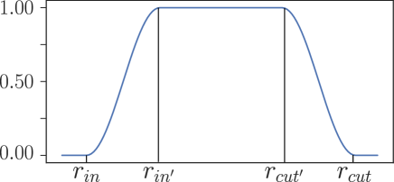
Figure 3: Two-sided cutoff function $f_{\rm cut}^{2s}$ with cutoff radii $r_{\rm cut},r_{\rm in}$, and parameters $r_{\rm cut}^{\prime},r_{\rm in}^{\prime}$.

For the two-body components, we start by solving the linear least-squares problem with the two-body components defined on the whole interval $[0,r_{\rm cut})$. We choose a splining point $r_{\rm S}$ that is sufficiently small so as to not influence the training set error, specific values are given in the following section. The new two-body components with repulsive core are defined such that

$$\begin{split}\tilde{E}_{2}(r)&:=\begin{cases}E_{2}(r),&r\geq r_{\rm S},\\ E_{\rm rep}(r),&r<r_{\rm S},\end{cases}\\ E_{\rm rep}(r)&=e_{\infty}+\beta r^{-1}e^{-\alpha r},\end{split}$$ (9)

where $e_{\infty}<E_{2}(r_{\rm S})$ is a parameter adjusting the steepness of the potential, and $\alpha,\beta$ are chosen such that $\tilde{E}_{2}$ is continuous and continuously differentiable at $r_{\rm S}$.

Note that the regularised least-squares problem is still linear, hence the regularisation procedure does not affect the computational cost of the fit.

III Methods

III.1 Fits and hyper-parameters

We now describe the details of the fitting process and training data generation to construct aPIPs for molecules. As detailed in Section IV, we explore the use of aPIPs for fitting the PES of individual molecules (trained and tested independently from one another), as well as for fitting a combined force field. The combined force field is fit to data from multiple linear hydrocarbons, and is then shown to be accurate for both the molecules it has been fit to as well as to slightly longer linear hydrocarbons. We used the same hyper-parameters in all fits, as shown in Table 2, except for the individual N-methylacetamide PES which was fit with a 4B maximum degree of 6 and the combined force field which used a cutoff of $r_{\rm cut}^{\prime}$ = 2.75 and $r_{\rm cut}$ = 3.25Å. For N-methylacetamide, as there are four different elements present, the number of basis functions is very large when the maximum degree for the 4B term is 10. Therefore, a lower maximum degree was used in this case to reduce the number of basis functions and still allow a potential to be fit for NMA with only 1000 structures. When performing individual molecule fits, the performance of the potential is relatively insensitive to the choice of outer cutoff. However, for the combined fit reducing the outer cutoff resulted in improved performance on the testing set.

When fitting individual molecular PESs, the hyperparameters could be optimised anew for each molecule and this would no doubt improve accuracy, but we are more interested in using a generic parameter set which does not need to be tuned and greatly reduces the effort required to create new fits. The fact that the resulting PESs are still very accurate suggests that the potentials could be made transferable across molecules. The potentials created include all possible 2B, 3B, and 4B terms; e.g. for butane, the 4B terms are HHHH, CHHH, CCHH, CCCH, CCCC. Not including some of these would result in a smaller number of basis functions and in some cases may not influence the accuracy of the potentials, for example one might surmise that the HHHH terms are not necessary. However, we have included all terms in our fits in order to eliminate the necessity of such manual choices.

The number of basis functions depends on the number of different elements, the maximum body order and polynomial degree. By way of example, the alkane fits in this work (beyond butane) use 13629 basis functions.

Parameter	Symbol	Value
Max degree-2B	$D_{2}$	12
Max degree-3B	$D_{3}$	10
Max degree-4B	$D_{4}$	10
Outer Cutoff	$r_{\rm cut}^{\prime},r_{\rm cut}$	4.00, 5.50 Å
Inner Cutoff	$r_{\rm in},r_{\rm in}^{\prime}$	0.70, 0.80 Å
Weight-Ratio	$W_{E}:W_{F}$	100:1
Regularisation	$\gamma_{n}^{{\bm{Z}}}$	0.05
Radial transform	$u$	$e^{(-2.5(r/1.54-1))}$

$r_{\rm S}$ (Å) CC: 0.93 CH: 0.56 HH: 0.27 CO: 0.98 OH: 0.61 NO: 1.02 NC: 0.96 NH: 0.59 OO: 1.04 NN: 0.99

Table 2: The hyperparameters used for fitting the aPIPs. The $r_{\rm S}$ values that define the switch-over to a repulsive core, $E_{\rm rep}$, in (9), correspond roughly to the point where the ZBL potential is 20 eV.

III.2 MD Training Data

The majority of the training data in our fits is obtained by taking snapshots from MD trajectories with a temperature of 1500K. To reduce the computational cost, these MD simulations were performed using DFTB Elstner et al. (1998) with the mio–1–1 parameter set, using the NVT ensemble with a Langevin thermostat and a friction coefficient of 0.002. The time step was 0.1 fs and samples were taken 1000 time steps apart. A total of 1000 structures were collected for each molecule, except for ethanol and N-methylacetamide, where the temperature was reduced to 800 K to prevent bond dissociation. We emphasise that with a fixed sized basis set, we expect convergence of the coefficients and thus a large number of data points were collected to ensure that. The evaluation cost of the aPIPs force field is independent of the number of training data points. We made no attempt to study the minimum size and composition of the optimal training set, this is left for future work. Energy and force data for the force field fit was then obtained by reevaluating the snapshots from the DFTB-MD using Molpro Werner et al. (2019) with a B3LYP hybrid DFT functional Stephens et al. (1994); Lee et al. (1988); Becke (1993) and 6-31G** basis set.

III.3 Additional Training Data

In addition to the high temperature MD, there are two more sources of training data that take account of the special structure of PESs. The first issue is that the repulsive potential (9) we add at small distances is not designed to accurately reproduce the potential energy, rather it is kept simple in order to ensure that it is repulsive and does not introduce additional local minima. This means that the splining point $r_{S}$ at which it is turned on is chosen well below the distance which we expect to encounter between atoms even at the high temperature of 1500K. The smooth transition to the repulsive potential is thus aided by manually adding dimer configurations of each pair of elements to the data set. One choice would be to use the same level of quantum mechanics for these as for the rest of the data set, but we opt instead to use the ZBL functional Ziegler et al. (1985), which is fit to Hartree–Fock data and has better accuracy than DFT at small distances. This ZBL set consists of 55 dimers with interatomic distances in the range of [0.1 Å,5.50 Å]. In the least squares fit, we reduce the weight if the ZBL set in a ratio of 100:1 relative to the rest of the training set, so that the ZBL data does not noticeably influence the accuracy of the fit in regions of configuration space where other data exists.

The second additional training data concerns only the molecules butene and ethene. The HCCH dihedral around the double bond in these molecules will not be sampled during the MD simulations as the energy barrier is too high. Therefore, the HCCH dihedral energy scans around the double bond are added to the training set, with 12 data points in each scan. The weight of this dihedral scan data is increased in the ratio 2:1, to take into account of the small number of samples in this additional data set.

III.4 Iterative Fitting Process

One of the key goals in using aPIPs is that “holes” in the potential should be eliminated. We consider any region of configuration space a hole which has lower energy than the energy of the molecule’s locally optimized structure when starting from the true equilibrium geometry. The presence of holes in PIP fits are well documented Nandi et al. (2019), and many overparametrised ML models are also in danger of having holes due to the high dimensionality of the molecular representation they use. In order to try and eliminate holes, we introduce an iterative fitting process that systematically searches for holes in configuration space. Various iterative fitting methods exists, with either geometry optimisation Deringer and Csányi (2017); Bernstein et al. (2019), MD or Diffusion Monte Carlo (DMC) Debiec et al. (2016); Nandi et al. (2019) used to sample the PES. Alternatively, active learning can be used, where the uncertainty of the prediction for a set of test structures is quantified and the most uncertain structures are added to the training set Gubaev et al. (2019); Smith et al. (2019). The dimensionality of our energy terms is much smaller than in the cases of the cited works, and so we opt for a different strategy. Using the Sobol quasirandom sequence Niederreiter (1988), we create a “Sobol test set” for each molecule according to the following procedure:

• The optimized structure of the molecule is calculated with the B3LYP hybrid functional and 6-31G** basis set, and the geometry is converted to internal coordinates.

• A Sobol sequence of length 100,000 is then produced with a dimension equal to the number of internal coordinates.

• The elements in the sequence correspond to the displacement of the internal coordinates from their equilibrium position, scaled such that the range of bond lengths, angles and dihedral displacements for non-cyclic molecules is $\pm 0.30$ Å, $\pm 10^{\circ}$ and $\pm 10^{\circ}$ respectively, for cyclic molecules these ranges are halved. Rotatable dihedrals are identified and allowed to take a value between 0-360^∘.

• The scaled Sobol sequence displacement vectors are then used to generate the set of 100,000 “Sobol test set” structures.

• Finally, we check for clashing atoms: any structure with atoms closer than the corresponding $r_{S}$ (see Table 2) is removed from the set.

The resulting Sobol test set has a diverse range of structures that sample the space around the equilibrium position more uniformly than if we did stochastic sampling. It is very fast to generate and does not rely on carrying out MD or DMC with either DFT or even a preliminary force field. Doing the latter could lead to poor results because the trajectory can get trapped in a hole, or result in bond dissociation.

The entire fitting process is summarized in Figure 4. In each iteration, the potential energy of the Sobol test set is calculated using the current force field. DFT calculations are performed for the five lowest energy structures, and up to five highest energy structures (with energies above 2.5 eV/atom), and added to the training set in the next iteration. This process is repeated until there are no structures with an energy below that of the equilibrium structure.

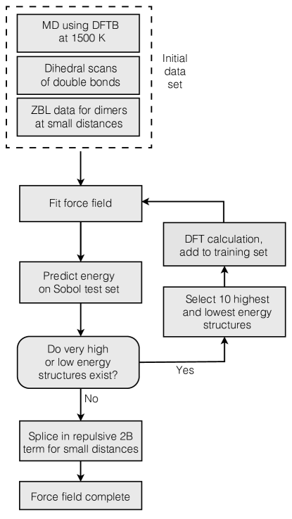
Figure 4: The flowchart shows the stages we used to build the database and fit the aPIP force field.

III.5 Empirical Force Field Comparison

To demonstrate the improved performance of aPIPs over an empirical force field, we parametrised a simple force field for methane on the same training set. The maximum body order is five, but the functional form is very limited and the number of free parameters is very small. The precise form for the empirical force field is given by,

$$\small\begin{split}&E=\sum_{bond}[K_{b2}(b-b_{0})^{2}+K_{b3}(b-b_{0})^{3}+K_{b4}(b-b_{0})^{4}]\\ &+\sum_{angle}[K_{a2}(\theta-\theta_{0})^{2}+K_{a3}(\theta-\theta_{0})^{3}+K_{a4}(\theta-\theta_{0})^{4}]\\ &+\sum_{bond/bond}K_{bb}(b-b_{0})(b^{\prime}-b^{\prime}_{0})\\ &+\sum_{bond/angle}K_{ba}(b-b_{0})(\theta-\theta_{0})\\ &+\sum_{angle/angle}K_{aa}|(\theta-\theta_{0})(\theta^{\prime}-\theta^{\prime}_{0})|\\ \end{split}$$ (10)

The parameters were determined by minimizing the functional given in Equation (6). The $W_{E}$ and $W_{F}$ terms in Equation (6) were the same as those used for the aPIP potential. For simplicity and given the simple functional functional form and large amount of data used, no regularization was needed in this case.

IV Results

IV.1 Convergence: tests on methane

Before we discuss the aPIP force field’s performance for a set of small molecules, we first examine its convergence properties, tradeoff between speed and accuracy as controlled by the basis set size, and the effects of regularisation and the iterative fitting process, all for the case of the individual fit to methane. Figure 5 shows the decrease in the energy root mean square error (RMSE) with the increasing number of basis functions and body order. The number of basis functions is dependent both on the maximum polynomial degree and body order, and for a fixed body order, the RMSE levels off to the minimum error possible for that body order. The minimum error for 3B is about $2\times 10^{-3}$ eV/per atom, and increasing the body order to 4B without changing the overall number of basis functions results in a big drop in the RMSE. In contrast, this is not the case for the empirical force field, for which there is very little gain beyond adding 3B terms.

In the Supplementary Information, we show that the distance-based coordinates are less accurate than the distance-angle coordinate system. The decision to use distance-angle coordinates for our force field is further strengthened by the results shown in S2, with the normal mode recreation for butene significantly better. The convergence of additional properties with the number of basis functions is discussed further in S2.

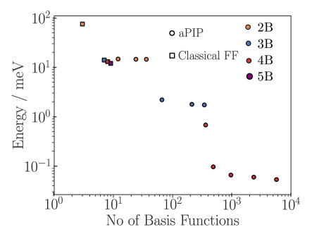
Figure 5: The change in the training set RMSE with the number of basis functions and body order for the methane aPIP potential (circles), up to body-order 4. Also shown are the errors of an empirical potential fit as the corresponding bond, angle etc terms are added (squares), up to body-order 5.

Although, as stated in the introduction, the aPIP formulation is the bridge between the low body order empirical force fields and high dimensional ML potentials, from the point of view of number of degrees of freedom we are interested in the regime when it is closer to the latter. Having thousands of degrees of freedom means that regularising the least squares fit is necessary in order to avoid overfitting. The regularisation effect is shown in Fig. 6. For the unregularised potential, the test set RMSE is about a 100 times larger than the training set RMSE.

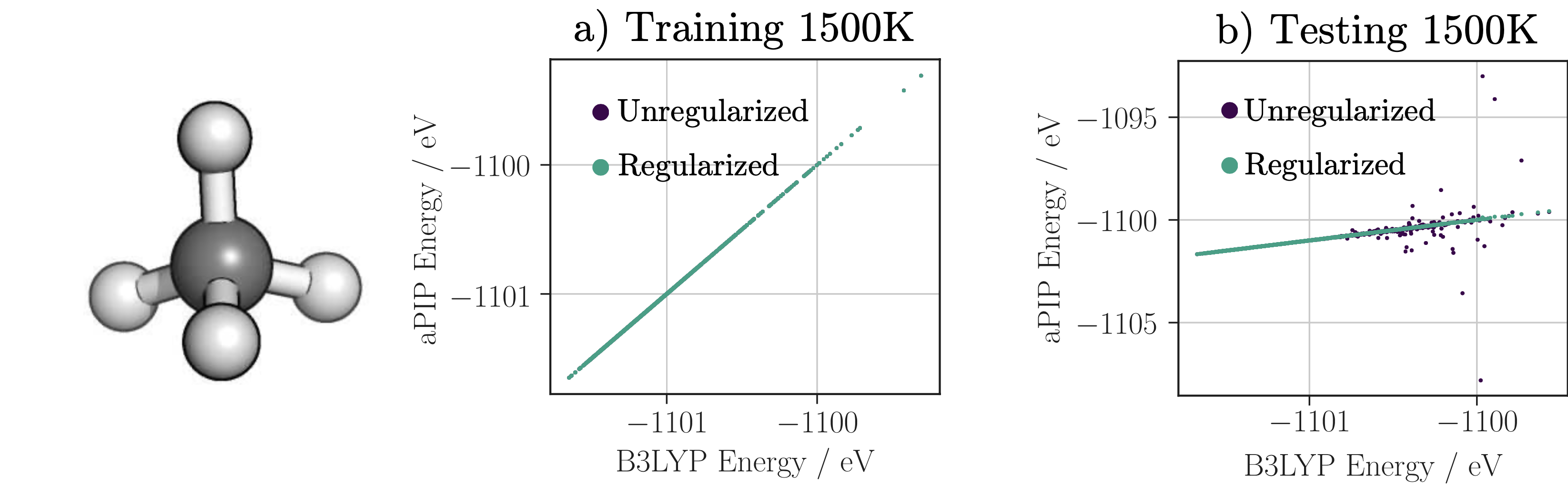
Figure 6: Comparison of target and predicted energies for the training and test sets, for both regularised and unregularised fits.

Figure 7 shows the effect of changing the regularisation strength $\gamma$ on the RMSE on the training and test sets. The training set is as described in the previous section, ZBL data and the iterative structures for the regularized fit are included in all potentials, whereas the test set is composed of 8000 independently sampled structures from the same 1500K MD simulation. For methane, the optimal regularization strength is at approximately 10^-4. The training set RMSE is relatively constant up until $10^{-2}$ when an increase starts. Given that we opted to use a single value for fitting all molecules in this paper, the higher regularisation strength of 0.05 is used, because for larger molecules that is beneficial due to the larger number of basis functions.

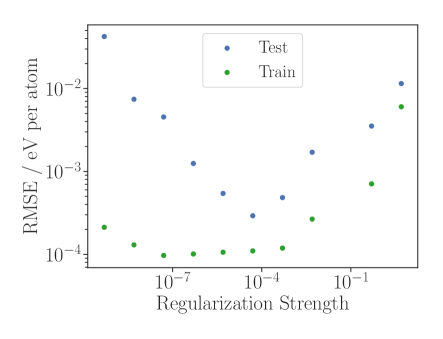
Figure 7: The energy RMSE of methane on the 1500K training and test set (8000 structures) as a function of regularization strength ($\gamma_{n}^{{\bm{Z}}}$).

Finally, Fig. 8 shows the RMSE as a function of the number of configurations in the MD training set (with no additional data), with the other parameters as in Table 2. The decrease in RMSE on a fixed test set of 1000 independent structures shows no sign of saturation, and reaches $1\times 10^{-4}$ for 8000 training configurations. We kept the regularisation strength fixed here, but if it were optimised separately for each training set size, the error would go down further and the difference between the errors on the training and test set be also naturally further reduced.

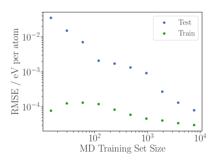
Figure 8: Energy RMSE of methane on a the 1500K training and test set (1000 structures) as a function of the MD sampled training set size. All other parameters are as in Table 2. Note that the errors at 1000 training structures are slightly higher than in Table 3 because the the potentials reported there include additional training data.

IV.2 Iterative Fitting

In Section III.4 we introduced an iterative fitting algorithm that samples structures derived using the Sobol quasirandom sequence. Figure 9 demonstrated the effect of a single iteration on the energy distribution on the Sobol test set. The original fit (labelled “Iter 1” in the figure) resulted in thousands of structures having a lower energy than the true equilibrium structure. The addition of just five of the lowest energy structures results in a considerable change in the energy distribution seen at the second iteration and all the structures with unrealistically low predicted energies disappear.

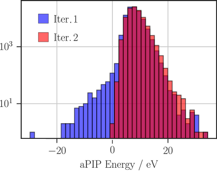
Figure 9: The energy distribution of the Sobol test set for the butane aPIP potential at iteration 1, and iteration 2 (trained with five additional Sobol test set structures). The energy is shifted so that true geometry optimised butane molecule is at 0.0 eV.

IV.3 Individual Molecule Force Fields

In this section, the performance of the aPIP force fields with up to 4-body terms for individual molecule PESs is evaluated for 14 small organic molecules. A combined fit to alkanes is discussed in the next section. Although ultimately we are interested in general force fields, considering the individual fits is interesting for a number of reasons. It enables comparison to other models that also target PESs one at a time (such as the PIP scheme and sGDML). Characterising the lowest possible error within a given body order and polynomial degree for individual fits is helpful when thinking about the errors of a general force field because it informs us of the extent to which the combined fit is forced to make compromises between fitting to data corresponding to different molecules.

IV.3.1 RMSE for Training and Testing Set

A most basic test of the performance of a force field is the RMSE of the energies for a training and testing set. Table 3 summarises the energy RMSE for the 14 molecules tested, further graphs are given in the Supplementary Information S1. We show total energy errors, and also error/atom, because as molecules get larger, we expect (when keeping the training set size constant) that the total energy error would go up, but the error/atom stay bounded. The table shows that this is mostly true, the test set error/atom stays near or below 3 meV/atom for molecules with only single bonds, and below 5 meV/atom for molecules with double bonds.

		Energy RMSE (meV)
Molecule	Atoms	Train 1500K*	Test 300K	Test 1500K*
Regularised 4-body aPIP
(individual molecule fits)
Methane	5	0.3	0.2	1.6 (0.3)
Ethane	8	1.8	1.2	7.8 (1.0)
Propane	11	3.0	2.9	12.7 (1.2)
Butane	14	8.2	7.0	29.1 (2.1)
Pentane	17	12.8	13.0	50.1 (2.9)
Hexane	20	19.6	28.1	65.8 (3.3)
Adamantane	26	11.5	4.1	22.0 (0.8)
Ethene	6	3.0	2.1	21.9 (3.7)
Butene	12	13.3	16.0	56.9 (4.7)
Butadiene	10	7.9	5.2	31.5 (3.2)
Benzene	12	4.3	1.9	8.8 (0.7)
Methylbenzene	15	8.5	4.1	25.7 (1.7)
Ethanol	9	*3.3	1.4	*5.6 (0.6)
NMA	12	*4.0	1.8	*4.6 (0.4)
mean		7.2	6.3	24.6 (2.2)
Unregularised 4-body aPIP
(individual molecule fits)
median		4.4	3.4	211
mean		5.3	$10^{6}$	$10^{8}$
maximum		16	$10^{7}$	$10^{9}$
Combined 4-body aPIP fit
Methane	5	4.38	0.98	3.47 (0.7)
Ethane	8	8.27	2.85	12.25 (1.5)
Propane	11	17.58	8.19	22.35 (2.0)
Butane	14	23.78	10.54	30.65 (2.2)
Pentane	17	26.15	16.94	44.27 (2.6)
Hexane	20	31.16	24.36	65.90 (3.3)
Heptane	23	-	35.06	118.36 (5.1)
Octane	26	-	44.84	156.62 (6.0)

Table 3: The RMSE of the energies for training and test sets is given for the fourteen molecules tested. The higher temperature testing set is taken from 1500K MD for all molecules, except ethanol and NMA (marked by *) where it is 800K, this is due to bond dissociation occurring for the higher temperature. Energy errors per atom are shown in parentheses.

Table 3 also shows that the 300K test set RMSE is comparable to the training set error. The configurations sampled by the 300K MD will be well within the sample of structures that the potential is fit to and are therefore well reproduced by the aPIP potential. The error for the higher temperature MD test set is several times higher than the training error. This is because structures that are not well represented by the training data will be present in the higher temperature MD. As discussed in Section IV.1, an increase in the number of structures in the training set will result in a decrease in the test set error (and this was demonstrated for methane). With a fixed body order and basis set size, there is of course a saturation to a minimum error. As an example, when a fit is made to butane with the same parameters but 10,000 training structures instead of 1000, the energy RMSE for the 1500K test set falls by 20% to 22.7 meV, a substantial decrease, but not as large as that for methane. There is no expectation that the rate of convergence is the same for different sized molecules. A detailed study of convergence rates for different molecules is left for future work.

IV.3.2 Comparison to Empirical Force Fields

In order to directly assess the enhanced accuracy of the aPIP model over empirical force fields of the same body order, we parametrised one for methane as described in Section III.5. The key differences between the two potentials are summarised as follows:

• The functional form used for aPIP is significantly more complex than for the empirical force field, with the number of degrees of freedom being 5694 and 9, respectively.

• The empirical force field includes only terms describing the interactions between atoms joined together by covalent bonds, whereas aPIP also naturally allows terms with nonbonded atoms (as long as they are within the spatial cutoff), e.g. the four-body HHHH term.

• The empirical force field includes a five-body term (the angle-angle coupling) whilst the aPIP presented here is limited to four-body terms.

Table 3 shows that the energy RMSE of the empirical force field for methane decreases significantly as the body order is increased up to 3B; 4B and 5B terms each bring less than 15% improvement. Compare this with the case of aPIPs (Fig. 5), where a decrease in error of almost a factor of 50 is possible when going from 3B to 4B. The final test set errors are about 40 times larger for the empirical force field than for aPIP, at both 300K and 1500K. This strongly suggests that it is the constraints of the functional form, rather than low body order that limits the accuracy of empirical force fields. Note however, that the training and test set errors of the empirical force field are nearly the same, even though no regularisation was used in its fit—the need for careful regularisation is the price one pays for introducing enormous flexibility in the functional form.

IV.3.3 Comparison to high dimensional methods

The aPIPs basis was introduced as a way to bridge the gap between empirical force fields and recent high dimensional machine learning based approaches. Therefore it is important to ask whether the limited body order aPIPs basis can reach the high accuracy of the ML methods, and at what computational cost. While we leave the detailed comparative study (including training and testing all methods on exactly the same data sets, optimising hyperparameters and computational efficiency of aPIPS, etc.) to future work, we can broadly answer in the affirmative. Methane and N-methyl acetamide (NMA) have both been fitted with the PIPs of Braams and Bowman. In Ref. Nandi et al. (2019), energy RMSE of 0.4 meV was achieved on the training set of 1000 methane structures. For NMA, Ref. Qu and Bowman (2019) gives the errors as 3.32 meV for the energy with the PIPs while the RMSE of the “fragment method 2” in that paper was 4.25 meV.

For the benzene and ethanol molecules, the performance of aPIP can be compared to the sGDML Chmiela et al. (2018). The energy RMSEs achieved there for a 500K test set are 5.2 meV and 3.9 meV, for benzene and ethanol, respectively. The corresponding errors for the 4-body aPIPs for the 1500K test set are about 30% higher.

IV.3.4 Bond, Angle and Dihedral Energy Scans

We now demonstrate that the combination of low body order and regularisation results in smooth potential energy surfaces up to very high energies, several eV higher than the equilibrium energy, which are never encountered in the 1500K training and test sets. We performed bond, angle and dihedral scans for each molecule. The full set of results are given in Supplementary Information S1.

The bond and angle aPIP energy scans show excellent agreement with the DFT results. The greatest differences between the aPIP and DFT scans occur for the hexane, butadiene and butene, which have more varied interactions and bonding present. However, even for these three molecules the energy scans are very well recreated. This level of accuracy for aPIP is in large part due to regularization. Figure 10 demonstrates this with a C–C–H angle energy scan for butene. The regularised aPIP curve with regularization exactly follows the DFT energy scan, whilst the unregularised aPIP fit results in unphysical oscillations.

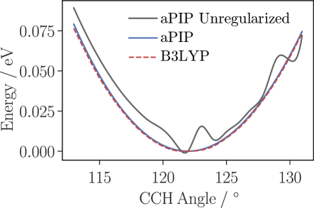
Figure 10: Energy curve for a C–C–H angle in the molecule butene. Results for aPIP with and without regularization are shown.

We also calculated the energy curve for dilating adamantane van Duin et al. (2001). Instead of just calculating the energy with the change in length of one individual bond, this test involves the uniform expansion of all the C–C bonds in adamantane. Again, a very close match with the DFT result is achieved. Note that adamantane has 26 atoms, this is over twice the size of N-methylacetamide, the largest molecule fit with PIPs Qu and Bowman (2019). The fragmentation approach developed in Ref. 29 would not be suitable for adamantane, as the cyclic structure means that unambigous fragments do not exist and therefore, without the reduction in body order achieved with aPIPs, it would not be possible to create a PIP potential for this molecule.

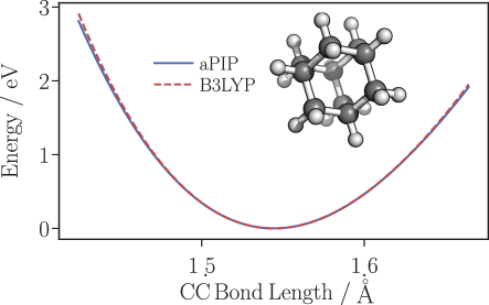
Figure 11: The energy curve for dilating adamantane, this is the uniform increase of the C–C bond length.

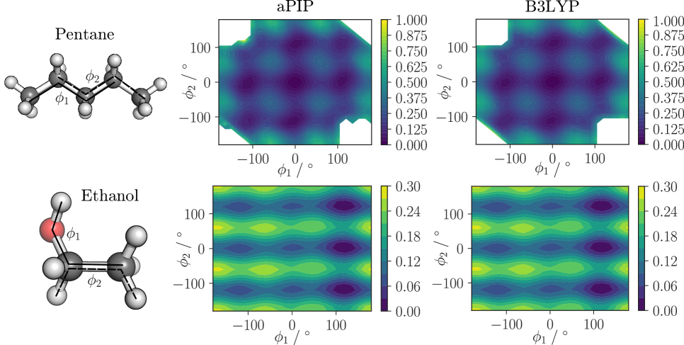
Figure 12: The 2D dihedral angle energy scans for pentane and ethanol. The dihedral angles changed are marked on the molecule. The energy units are eV and values above 1.0 eV are not shown on the plot.

Accurate dihedral energy scans are an essential criterion for any organic molecular force field, and so a variety of dihedral angle energy scans for the aPIP potentials are shown in S1. The DFT energy is generally well reproduced. Hexane again shows slight discrepancy, with a RMSE of 26.7 meV, similar to the RMSE on the 300K test set.

Further tests of aPIP’s ability to reproduce dihedral effects is shown in the two dimensional maps of Fig. 12. For both pentane and ethanol, minimum and maximum energy barriers are reproduced and the high energy regions in the DFT pentane map also occur in the aPIP map. One of the interesting points to note about the aPIP pentane potential is that before the Sobol structures are added to the training set through the iterative fitting process, the high energy regions of the 2D energy scan contain an unrealistically low energy structure, as shown in Fig. 13. At the first iteration of the fitting algorithm the RMSE for the 2D scan is 159 meV, whilst at the last iteration the RMSE is 36.6 meV, with the remaining error primarily due to the structures in the high energy region.

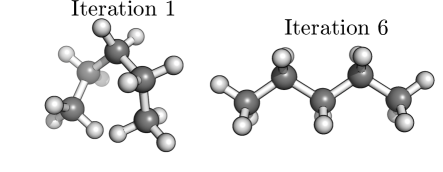
Figure 13: The lowest energy structure in the pentane 2D dihedral energy scan with the aPIP pentane potential at iteration 1 and at iteration 6.

As a final example of the dihedral energy scan recreation, we show the energy scan of the methyl group attached to the N–C bond in NMA in Figure 14. The DFT energies and barrier heights are very well reproduced, and this along with the graphs shown in Supplementary Information S1 demonstrate the success of aPIPs for a molecule with four different element types.

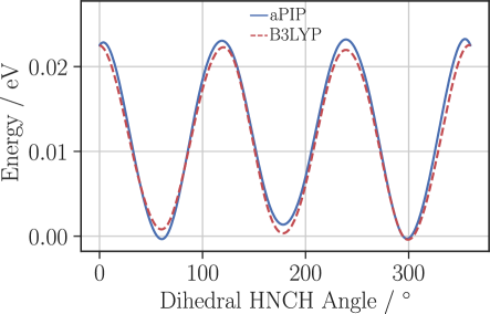
Figure 14: The dihedral energy scan for the methyl group attached to the N–C bond of NMA.

IV.3.5 Normal Mode Recreation

Vibrational frequencies of molecules are regularly used as a measure of the accuracy of a force field. Empirical force fields with Class I functional forms, which have harmonic bond/angle terms and no coupling terms i.e. AMBER or OPLS, can achieve an error in the recreation of frequencies of approximately 50 ${\rm cm}^{-1}$ Allen et al. (2018) (mean absolute error, MAE) whilst Class II force fields, which include anharmonic and coupling terms in their functional forms, can achieve an MAE around 24 cm^-1 Ewig et al. (2001).

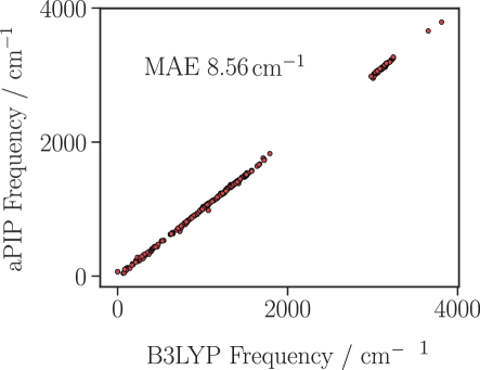
Figure 15: The DFT and aPIP normal mode frequencies for the set of 14 molecules. The mean absolute error (MAE) for the normal mode recreation is 8.56 cm^-1.

The normal mode recreation for each individual molecule is given in S1 with all the DFT and aPIP frequencies for the molecules tested shown in Fig. 15. With a MAE of 8.56 cm^-1 for the full set of molecules, aPIP recreates the normal mode frequencies with an accuracy that is far superior to empirical force fields. The individual molecules figures in S1 show that ethene has the highest MAE (16.6 cm^-1) whilst methane has a very low error with a MAE of just 0.647cm^-1.

IV.4 Combined Molecule Potentials

In this section, we show that the aPIP framework allows multiple molecules to be fit simultaneously, just as empirical force fields do. This is in contrast to some high dimensional methods such as PIPs and sGDML.

	Frequency
	MAE (cm-1)
	Individual	Combined
Methane	0.647	10.76
Ethane	4.93	10.76
Propane	4.8	13.71
Butane	10.65	16.88
Pentane	11.04	15.77
Hexane	15.06	17.72
Heptane	-	19.69
Octane	-	21.67

Table 4: The normal mode recreation errors for the combined and individual aPIP potentials for a set of short linear alkanes. The training set includes the linear alkanes up to hexane.

Table 3 shows the testing and training RMSE for the aPIP model fitted to the combined training set of linear alkanes up to hexane. This can be compared to results for the individual aPIP fits in the same table. For alkanes with up to four carbon atoms, the individual molecule fits are superior. However, even for these four molecules the combined fit RMSE remains below 3 meV/atom on the high temperature test set. For pentane and hexane the combined fit gives the same or better levels of accuracy compared with the individual fits. Additionally, closer agreement between the training and test set RMSE is observed for the combined fit. This is due to the increase in the number and diversity of structures in the training set which further reduces overfitting.

Table 4 showing the normal mode recreation exhibits a similar trend to the RMSE results. The error for shorter linear alkanes is lower with the individual aPIP potentials, but as the alkanes become longer the difference between the individual and combined aPIP potential errors decreases. The error in the combined molecule fit is still far below the typical errors expected from empirical force fields.

The extrapolation capabilities of the combined potential to molecules not included in the fitting set are also demonstrated in Tables 3, 4 and Fig. 16. The RMSE for the 300 K testing set increases for the heptane and octane molecules, but stays below 2 meV/atom. The 1500 K test set RMSE shows a greater increase and demonstrates the need for larger data sets and possibly larger cutoffs. The normal mode recreation error for heptane and octane (Table 4) remains acceptable, with the error increasing only by 3.96 cm^-1 from hexane to octane. Figure 16 examines the energy scans for heptane. The CCH energy scan is reproduced very well and the overall shape of the CCCC dihedral energy scan is also reasonable. However, the trans-gauche dihedral energy barrier is 0.03eV lower than the corresponding DFT value.

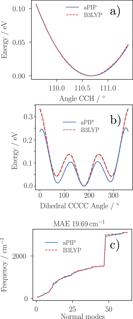
Figure 16: a) CCH angle and b) CCCC dihedral energy scans and normal mode recreation for heptane, which was not the training set.

Currently, the best transferable high dimensional force field is ANI Smith et al. (2017, 2018, 2019). While a detailed comparative study is left for future work, the DFT version (ANI-1) gives RMSE errors on the GDB-11 database of about 2.9 meV/atom Smith et al. (2017), higher than what the combined 4-body aPIP fit achieves on our limited range of molecules.

V Discussion and Conclusion

In this work, we have built on the ideas introduced in Ref. 54, which reformulated the permutationally invariant polynomial basis for single element materials, and created potentials for organic molecules using the multi-element atomic permutationally invariant polynomial (aPIP) basis. We showcase potentials that restrict the body order (in the present case to four), and employ a bond-angle based coordinate system, cutoffs for large and small distances, a repulsive core, and regularize the least square fitting. These alterations allow potentials for much larger molecules to be created and multiple molecules to be fit at once, in contrast to the original PIP framework. Additionally, by a combination of regularization and iterative training, the “holes” in the potential are eliminated, making them suitable for molecular dynamics (see the SI for examples).

The performance of the aPIP potentials, both individually fitted to organic molecules and simultaneously to a combined set, showed very good accuracy for a number of properties (e.g. a few meV per atom error for the energy at 1500K), on a par with recent machine learning approaches. The speed of aPIP potentials is of course much slower than that of empirical force fields, but is the same order of magnitude as other ML potentials: typically on the order of 1 ms/atom. Fast implementations of polynomial bases exist (certainly for MTP Shapeev (2016b) and also ACE Drautz (2019); Bachmayr et al. (2019)) that will bring this time down further.

Furthermore, the relatively small dimensionality of low body order terms coupled with well controlled regularisation results in smooth potentials and remarkable extrapolation properties. Returning to Fig. 1, we see that the aPIP dissociation curves of methane are smooth and qualitatively correct, even though the only data that informs the potential are near equilibrium geometries, and the isolated atom energies. The latter only ensures that the simultaneous removal of all four Hs gives the correct limit at infinite distance (black dashed line in the bottom panel), the rest is extrapolation.

We have also outlined the relationships between the approaches for making force fields. Although each have rather distinct assumptions and seemingly incompatible mathematical frameworks, it turns out that body ordered polynomials (either the aPIPs variety used in this work, or the atomic cluster expansion) form links between them. This points the way forward to creating potentials that do not require atom typing, can be reactive and transferable, but remain highly accurate approximators of the Born-Oppenheimer potential energy surface.

Building a comprehensive organic force field is a significantly larger undertaking, but our limited results already show that achieving high accuracy does not necessarily need nonlinear fitting such as neural networks or even kernel methods. This, which we consider the main point of this work, is at variance with what might be gleaned from recent trends in the literature.

in 1,…,39 See pages \x of SI_aPIP_Molecules.pdf