Quantum Superposition Inspired Spiking Neural Network

SUMMARY

Despite advances in artificial intelligence models, neural networks still cannot achieve human performance, partly due to differences in how information is encoded and processed compared to human brain. Information in an artificial neural network (ANN) is represented using a statistical method and processed as a fitting function, enabling handling of structural patterns in image, text, and speech processing. However, substantial changes to the statistical characteristics of the data, for example, reversing the background of an image, dramatically reduce the performance. Here, we propose a quantum superposition spiking neural network (QS-SNN) inspired by quantum mechanisms and phenomena in the brain, which can handle reversal of image background color. The QS-SNN incorporates quantum theory with brain-inspired spiking neural network models from a computational perspective, resulting in more robust performance compared with traditional ANN models, especially when processing noisy inputs. The results presented here will inform future efforts to develop brain-inspired artificial intelligence.

INTRODUCTION

Many machine learning methods using quantum algorithms have been developed to improve parallel computation. Quantum computers have also been shown to be more powerful than classical computers when running certain specialized algorithms, including Shor’s quantum factoring algorithm [Shor, 1999], Grover’s database search algorithm [Grover, 1996], and other quantum-inspired computational algorithms [Manju and Nigam, 2014].

Quantum computation can also be used to find eigenvalues and eigenvectors of large matrices. For example, the traditional principal components analysis (PCA) algorithm calculates eigenvalues by decomposition of the covariance matrix; however, the computational resource cost increases exponentially with increasing matrix dimensions. For an unknown low-rank density matrix, quantum-enhanced PCA can reveal the quantum eigenvectors associated with the large eigenvalues; this approach is exponentially faster than the traditional method [Lloyd et al., 2014].

K-means is a classic machine learning algorithm that classifies unlabeled datasets into $k$ distinct clusters. A quantum-inspired genetic algorithm for K-means has been proposed, in which a qubit-based representation is employed for exploration and exploitation in discrete “0” and “1” hyperspace. This algorithm was shown to obtain the optimal number of clusters and the optimal cluster centroids [Xiao et al., 2010]. Quantum algorithms have also been used to speed up the solving of subroutine problems and matrix inversion problems [Harrow et al., 2009]; for example, Grover’s algorithm [Grover, 1996] provides quadratic speedup of a search of unstructured databases.

The quantum perceptron and quantum neuron computational models combine quantum theory with neural networks [Schuld et al., 2014]. Compared with the classical perceptron model, the quantum perceptron requires fewer resources and benefits from the advantages of parallel quantum computing [Schuld et al., 2015, Torrontegui and García-Ripoll, 2019]. The quantum neuron model [Cao et al., 2017, Mangini et al., 2020] can also be used to realize classical neurons with sigmoid or step function activation by encoding inputs in quantum superposition, thereby processing the whole dataset at once. Deep quantum neural networks [Beer et al., 2020] raise the prospect of deploying deep learning algorithms on quantum computers.

Spiking neural networks (SNN) represent the third generation of neural network models [Maass, 1997] and are biologically plausible from neuron, synapse, network, and learning principles perspectives. Unlike the perceptron model, neurons in an SNN accept signals from pre-synaptic neurons, integrating the post-synaptic potential and firing a spike when the somatic voltage exceeds a threshold. After spiking, the neuron voltage is reset in preparation for the next integrate-and-fire process. SNN are powerful tools for representation and processing of spatial-temporal information. Many types of SNN have been proposed for different purposes. Examples include visual pathway-inspired classification models [Zenke et al., 2015, Zeng et al., 2017], basal ganglia-based decision-making models [Héricé et al., 2016, Cox and Witten, 2019, Zhao et al., 2017], and other shallow SNN [Khalil et al., 2017, Shrestha and Orchard, 2018]. Different SNN may include different types of biologically plausible neurons, e.g., the leaky integrate-and-fire (LIF) model [Gerstner and Kistler, 2002], Hodgkin–Huxley model, Izhikevich model [Izhikevich, 2003], and spike response model [Gerstner, 2001]. In addition, many different types of synaptic plasticity principles have been used for learning, including spike-timing-dependent plasticity [Dan and Poo, 2004, Frémaux and Gerstner, 2016], Hebbian learning [Song et al., 2000], and reward-based tuning plasticity [Héricé et al., 2016].

Quantum superposition SNN has theoretic basis in both biology [Vaziri and Plenio, 2010] and computational models [Kristensen et al., 2019]. From one perspective, spiking neuron models, such as the LIF and Izhikevich models, can be reformed by quantum algorithms in order to accelerate their processing using a quantum computer. On the other hand, quantum effects such as entanglement and superposition are regarded as special information-interactive methods and can be used to modify the classical SNN framework to generate similar behavior to that of particles in the quantum domain. In this work, we follow the latter approach. More specifically, we use a quantum superposition mechanism to encode complementary information simultaneously and further transfer it to spike trains, which are suitable for SNN processing. In our proposed quantum superposition SNN (QS-SNN) model, quantum state representation is integrated with spatio-temporal spike trains in SNN. This characteristic is conducive to good model performance not only on standard image classification tasks but also when handling color-inverted images. QS-SNN encodes the original image and the color-inverted image in the format of quantum superposition; the changing background context demonstrated by the spiking phase and spiking rate contains the image pixels’ identity information.

We combine quantum superposition information encoding with SNN for three reasons. First, the possible influence of quantum effects on biological processes and the related quantum brain hypothesis have been theoretically investigated [Vaziri and Plenio, 2010, Fisher, 2015, Weingarten et al., 2016]. Second, quantum superposition states are represented by vectors in complex Hilbert space, in contrast to traditional ANN, which operate in real space only; this is more representative of brain spikes, as the spiking rate and spiking phase spatio-temporal property also have complex number representation. In essence, SNN are more appropriate for quantum-inspired superposition information encoding. Third, current quantum machine learning methods, especially those used for quantum image processing, focus on encoding a classical image in the quantum state, with the image processing methods accelerated by quantum computing [Iyengar et al., 2020]. There has been less exploration of the possibility of using a quantum superposition state coding mechanism for different pattern information-processing frameworks. More importantly, owing to the use of statistical methods and fitting functions, current ANN show a huge performance drop when required to recognize a background-inverted image. This inspired us to develop a new information representation method unlike that used in traditional models. The integration of characteristics from SNN and quantum theory is intended to achieve a better representation of multi-states and potentially enable easier solving of tasks that are challenging for traditional ANN and SNN models.

The subsequent sections describe how complementary superposition information is generated and transferred to spatio-temporal spike trains. A two-compartment SNN is used to process the spikes. The proposed model, combining complementary superposition information encoding with the SNN spatio-temporal property, can successfully recognize a background color-inverted image, which is hard for traditional ANN models.

Complementary superposition information encoding

Quantum image processing

Quantum image processing combines image processing methods with quantum information theory. There are many approaches to internal representation of an image in a quantum computer, including flexible representation of quantum images (FRQI), NEQR, GQIR, MCQI, and QBIP [Iyengar et al., 2020, Mastriani, 2020], which transfer the image to appropriate quantum states for the next step of quantum computing. Our approach is inspired by the FRQI method [Le et al., 2011], as shown in Equations (1) and (2):

$$\mathinner{|I(\theta)\rangle}=\frac{1}{2^{n}}\sum\limits_{i=0}^{2^{2n}-1}(sin(\theta_{i})\mathinner{|0\rangle}+cos(\theta_{i})\mathinner{|1\rangle})\mathinner{|i\rangle},$$ (1)

$$\theta_{i}\in[0,\frac{\pi}{2}],i=1,2,3,\dots,2^{2n}-1,$$ (2)

where $\mathinner{|I(\theta)\rangle}$ is the quantum image, qubit $\mathinner{|i\rangle}$ represents the position of a pixel in the image, and $\theta=(\theta_{0},\theta_{1},\dots,\theta_{2^{2n}-1})$ encodes the color information of the pixels. FRQI satisfies the quantum state constraint in Equation (3):

$$\parallel\mathinner{|I(\theta)\rangle}\parallel=\frac{1}{2^{n}}\sqrt{\sum\limits_{i=0}^{2^{2n}-1}(cos^{2}\theta_{i}+sin^{2}\theta_{i})}=1.$$ (3)

Complementary superposition spikes

We propose a complementary superposition information encoding method and establish a linkage between quantum image formation and spatio-temporal spike trains. The complement code is widely used in computer science to turn subtraction into addition. We encode the original information and complementary information into a superposition state; one example is shown in Equation (4), with the rightmost sign bit removed and taking the complement:

$$\mathinner{|I(\theta_{i})\rangle}=cos(\theta_{i})\mathinner{|[0000001]_{b}\rangle}+sin(\theta_{i})\mathinner{|[1111110]_{b}\rangle}.$$ (4)

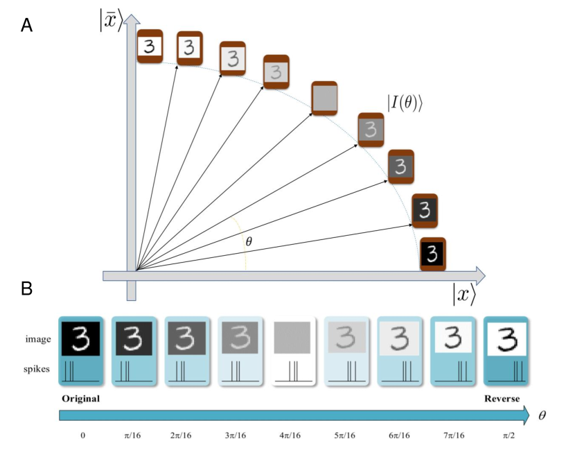
Figure 1: Quantum complementary superposition information encoding. (A) The horizontal axis and longitudinal axis represent $\mathinner{|x\rangle}$ and $\mathinner{|\bar{x}\rangle}$, respectively. The parameter $\theta$ in Equation (5) measures the degree to which the image background is inverted, from $\theta=0$ (the original image) to the complementary state $\theta=\frac{\pi}{2}$ (totally inverted background). (B) The top pictures show images inverted to different degrees, and the spikes to which they are encoded. The bottom axis corresponds to the value of $\theta$. It should be noted that the pictures are intuitive demonstration instead of exact display.

Equation (4) is an illustration of how complementary superposition information encoding works, with no factual significance. In this work, we focus on quantum image superposition encoding, as in Equation (5). However, it should be noted that any form of information that has a complement format, not just an image, can be encoded as a superposition state. Images in complementary quantum superposition states are further transferred to spike trains, as depicted in Figure 1. An image in its complementary state has an inverted background.

$$\mathinner{|I(\theta)\rangle}=\frac{1}{2^{n}}\sum\limits_{i=0}^{2^{2n}-1}(cos(\theta_{i})\mathinner{|x_{i}\rangle}+sin(\theta_{i})\mathinner{|\bar{x}_{i}\rangle})\otimes\mathinner{|i\rangle},\\$$ (5)

$$\theta_{i}\in[0,\frac{\pi}{2}],i=1,2,3,\dots,2^{2n}-1.$$ (6)

The complementary quantum superposition encoding is shown in Equations (5) and (6), where the $\mathinner{|i\rangle}$ represent pixel positions. Unlike FRQI, which uses qubits only for color encoding, here we use complementary qubits for encoding both original image pixels $x_{i}$ and the color-inverted image $\bar{x}_{i}$ with $\bar{x}_{i}=1-x_{i}$, supposing the pixel $x_{i}$ domain ranges from 0 to 1.0. The parameter $\theta_{i}$ represents the degree of quantum image $\mathinner{|I\rangle}$, mixing the original state $\mathinner{|x\rangle}$ and reverse state $\mathinner{|\bar{x}\rangle}$.

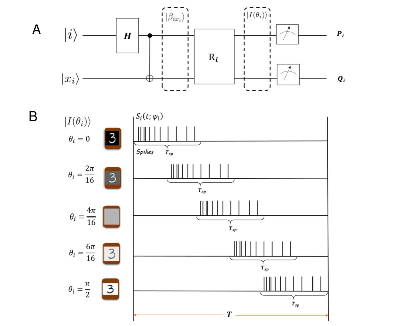
Figure 2: Quantum superposition spike trains. (A) The circuit to generate quantum image. Only one image pixel state is depicted for perspicuity. (B) A schematic diagram shows the transformation of quantum superposition states to spike trains $S_{i}(t;\varphi_{i})$. With parameter $\theta_{i}$ increasing, spike trains are shifted in time dimension. $T$ is a simulation period in which spikes emerge within the $T_{sp}$ time window. Also, the relation of parameter $\theta_{i}$ and spiking phase $\varphi_{i}$ is intuitive example and not exact correspondence.

We designed quantum circuit for the generation of quantum superposition image $\mathinner{|I(\theta_{i})\rangle}$ as shown in the figure 2(A), which is also discussed in [Le et al., 2011, Dendukuri and Luu, 2018]. The quantum state $\mathinner{|x_{i}\rangle}$ is processed by Hadamard transform $H$ and controlled $NOT$ gate to form the complementary state $\mathinner{|\beta_{ix_{i}}\rangle}$ with:

$$\mathinner{|\beta_{ix_{i}}\rangle}=\frac{\mathinner{|0,x_{i}\rangle}+(-1)^{i}\mathinner{|1,\bar{x}_{i}\rangle}}{\sqrt{2}},$$ (7)

Then rotation matrices $R_{i}$ is used to encode phase information as

$$R_{i}=\left[\begin{matrix}cos\frac{\theta_{i}}{2}&-sin\frac{\theta_{i}}{2}\\ \\ sin\frac{\theta_{i}}{2}&cos\frac{\theta_{i}}{2}\end{matrix}\right]$$ (8)

Finally, the superposition state $\mathinner{|I(\theta_{i})\rangle}$ is measured and two states are retrieved with probability $P_{i}$ and $Q_{i}$.

The complex information in quantum encoding is similar to signal processing in SNN. Neuron spikes can encode spatio-temporal information with specific spiking rates and spiking times, which can be used to represent quantum information.

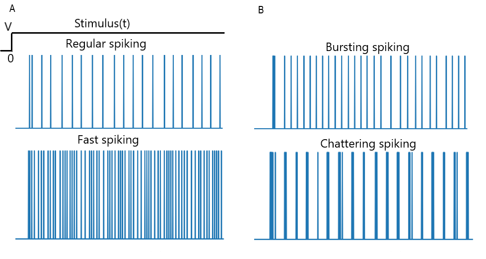
Figure S1: Spiking patterns with different fire rates or phases, Related to Figure 1. (A) Neurons fire at the same time but with different numbers of spikes generated per time unit. (B) Neurons fire the same number of spikes but the time of spiking is different.

Neuron spikes have the attribute of spatiotemporal dimension, which are identical in shape but differ significantly in frequency and phase, seeing Izhikevich neuron model [Izhikevich, 2003] in Figure S1, and are well-suited to the implementation of the vector form quantum image in Equation (5). We use spike trains with firing rate $r_{i}$ and firing phase $\varphi_{i}$ to represent quantum image state $\mathinner{|I(\theta_{i})\rangle}$. As shown in figure 2(A), the spike trains containing information of $\mathinner{|I(\theta_{i})\rangle}$ can be generated using Equation(9) and Equation (10).

$$r_{i}=\frac{\parallel\mathinner{|I(\theta)\rangle}\parallel-sin(\varphi_{i})}{cos(\varphi_{i})-sin(\varphi_{i})},$$ (9)

$$\varphi_{i}=\mathcal{F}\{arctan(\frac{P_{j}}{Q_{j}})|j=1,2,...,N.\},$$ (10)

Notation $\mathcal{F}\{X_{i}\}$ is set operation, and is specific in different tasks. The superposition state encoding $\mathinner{|I(\theta_{i})\rangle}$ is transferred to spike trains $S_{i}(t;\varphi_{i})$, which is generated from a Poisson spikes $S_{i}(t)$ with spike rate $r_{i}$ and extended phase $\varphi_{i}$ shown as Equation (11). Here, $T$ is the time interval of neuron processing spikes received from pre-synaptic neurons, and $T_{sp}$ is the spiking time window in this period, as shown in Figure 2(B):

$$S_{i}(t;\varphi_{i})=S_{i}(t-t_{0}),$$ (11)

$$t_{0}=\frac{\varphi_{i}}{\pi/2}*(T-T_{sp}).$$ (12)

Two-compartment SNN

Synapses with time-differential convolution

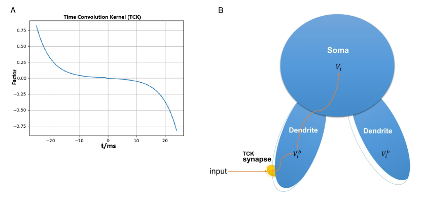
Figure S2: Two-compartment neuron mode,Related to STAR Methods. (A) Time convolution kernel. (A) Neuron with dendrite and soma compartments. Orange curve arrow shows information flowing from pre-synaptic input to dendrite potential $V_{i}^{b}$ and then integrated in soma potential $V_{i}$.

Synapses play an important part in the conversion of information from spikes in pre-synaptic neurons to membrane potential (or current) in post-synaptic neurons. In this work, the time-differential kernel (TCK) convolution synapse is used, as shown in Equations (13) and (14) and Figure S2. The spikes, $S_{i}$, from pre-synaptic neurons are convoluted with a kernel and then integrated with the dendrite membrane potential $V_{b}(t)$. This process can be considered as a stimulus-response convolution with the form of a Dirac function [Urbanczik and Senn, 2014]:

$$\left\{\begin{array}[]{l}\kappa(t)=\zeta(t)-\zeta(-t)\\ \zeta(t)=\Theta(t)(e^{-\frac{t}{\tau}})\end{array},\right.$$ (13)

$$V_{j}^{b}(t)=\sum\limits_{i}w_{i,j}\parallel\int_{-T}^{+T}\kappa(\tau)S_{i}(\tau)\,d\tau\parallel.$$ (14)

Two-compartment neurons

Both the hidden layer and the output layer contain biologically plausible two-compartment neurons, which dynamically update the somatic membrane potential $V_{i}(t)$ with the dendrite membrane potential $V^{b}_{i}(t)$, as shown in Figure S2.

In the compartment neuron model, $V_{i}^{h}(t)$ is the membrane potential of neuron $i$ in the hidden layer, which is updated with Equation (15); $g_{B}$, $g_{L}$, and $\tau_{L}$ are hyperparameters that represent synapse conductance, leaky conductance, and the integrated time constant, respectively; $V^{PSP}_{j}(t)$ is the synaptic input from neuron $j$; $V_{i}^{h,b}(t)$ is the dendrite potential with adjustable threshold $b_{i}^{h}$ in the hidden layer; and $w_{ij}^{h}$ is the synaptic weight between the input and hidden layers:

$$\left\{\begin{array}[]{l}\tau_{L}\frac{dV_{i}^{h}(t)}{dt}=-V_{i}^{h}(t)+\frac{g_{B}}{g_{L}}(V_{i}^{h,b}(t)-V_{i}^{h}(t))\\ V_{i}^{h,b}(t)=\sum\limits_{j}w_{ij}^{h}V^{PSP}_{j}(t)+b_{i}^{h}\\ V^{PSP}_{j}(t)=\parallel\int_{-T}^{+T}\kappa(\tau)S_{j}(\tau)\,d\tau\parallel.\end{array}\right.$$ (15)

The somatic neuron model in the output layer contains 10 neurons corresponding to 10 classes of the MNIST dataset. As shown in Equation (16), the hidden layer neurons deliver signals to the output layer with integrated spike rate $r_{i}$, which is differentiable; hence, it can be tuned with back-propagation. Here, $V_{i}^{o}(t)$ is the membrane potential in the output layer, $V_{i}^{o,b}(t)$ is the dendrite potential, and $r_{max}$ is the hyperparameter for rescaling of fire-rate signals:

$$\left\{\begin{array}[]{l}\tau_{L}\frac{dV_{i}^{o}(t)}{dt}=-V_{i}^{o}(t)+\frac{g_{B}}{g_{L}}(V_{i}^{o,b}-V_{i}^{o}(t))\\ V_{i}^{o,b}(t)=\sum\limits_{j}w_{ij}^{o}r_{j}(t)+b_{i}^{o}\\ r_{j}=r_{max}\sigma(V_{j}^{h})\\ \sigma(x)=1/(1-exp(-x)).\end{array}\right.$$ (16)

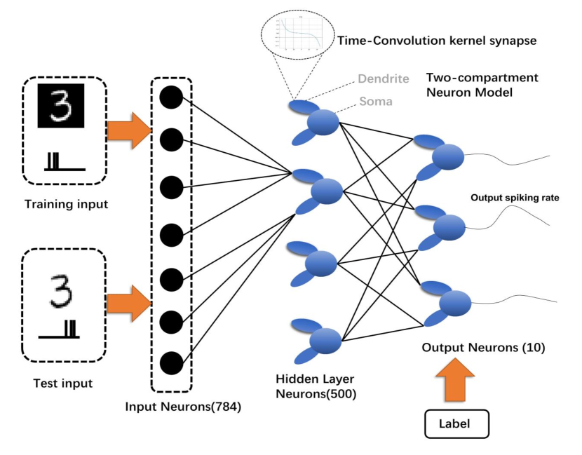
Figure 3: Quantum superposition SNN, three-layer architecture of QS-SNN with TCK synapses and two-compartment neurons. Images are transferred to spikes as network inputs. The hidden layer is composed of 500 two-compartment neurons with dendrite and soma. The output layer contains 10 two-compartment neurons corresponding to 10 classes. In the training period, only original images are fed to the network, whereas in the test period, the trained network is tested with inverted-background images. Neurons with maximum spiking rates at the output layer are taken as the network prediction and output.

The shallow three-layered architecture is shown in Figure 3. The input layer receives quantum spikes with encoding of complementary qubits. The hidden layer of QS-SNN consists of a two-compartment model with time-differential convolution synapses. Neurons in the output layer are integrated spike-rate neurons, which receive an integrated fire rate from pre-synaptic neurons, as well as the teaching signal $V_{I}$ as information about class labels.

Computational experiments

We examined the performance of the QS-SNN framework on a classification task using background-color-inverted images from the MNIST [LeCun et al., 2010] and Fashion-MNIST [Xiao et al., 2017] datasets. QS-SNN encodes the original image and its color-inverted mirror as complementary superposition states and transfers them to spiking trains as an input signal to the two-compartment SNN. The dendrite prediction and proximal gradient methods used to train this model can be found in STAR Methods.

For comparison, we also tested several deep learning models on the color-inverted datasets, including a fully connected ANN, a 10-layers CNN [Lecun et al., 1998], VGG [Simonyan and Zisserman, 2015], ResNet [He et al., 2016] and DeseNet [Huang et al., 2017]. All models are trained with original image $x_{i}$ and then tested on the background reverse image $I(\theta_{i})$. The only difference is that, for QS-SNN, quantum superposition state image $\mathinner{|I(\theta_{i})\rangle}$ is transferred to spike trains which is compatible with spiking neural networks. In other words, our essential idea is that the spatiotemporal property of neuron spikes enables the brain to transform spatially variant information into time differential information.

In this work, we formulated the spike trains transformation as the quantum superposition shown in Equation (5). And we have also demonstrated the numerical calculation of $I(\theta_{i})$ which is used for traditional ANN and CNN model testing in STAR Methods.

In addition, it is worth noting that the superposition state image $\mathinner{|I(\theta_{i})\rangle}$ is constructed from original information $\mathinner{|x_{i}\rangle}$ and reverse image $\mathinner{|\bar{x}_{i}\rangle}$. The original image and its complementary reverse information are maintained in the superposition state encoding $\mathinner{|I(\theta_{i})\rangle}$ at the same time. Because SNN is not processing pixel value directly, we transformed $\mathinner{|I(\theta_{i})\rangle}$ to spike trains, which can be regarded as different expression of superposition state encoding image in spatiotemporal dimension.

Standard and color-inverted images

The standard MNIST dataset contains images of 10 classes of handwritten digits from 0 to 9; images are 28x28 pixels in size, with 60,000 and 10,000 training and test samples, respectively. Fashion-MNIST has the same image size and the same training and testing split as MNIST but contains grayscale images of different types of clothes and shoes.

The original MNIST and Fashion-MNIST images and their color-inverted versions, with different degrees of inversion as measured by parameter $\theta$, are depicted in Figure 4(A) and (B), respectively. To be specific, the spiking phase estimating operation $\mathcal{F}\{X_{i}\}$ in Equation (10) is set as piecewise selection function as

$$\varphi_{i}=\left\{\begin{array}[]{l}arctan(\frac{P_{j}}{Q_{j}}),\quad j=i,\\ 0,\qquad\qquad\quad\ j\neq i.\end{array}\right.$$ (17)

Robustness to reverse pixel noise and Gaussian noise

Besides the effects of changing the whole background, we were interested in the capability of QS-SNN to handle other types of destabilization of images. For this purpose, we added reverse spike pixels and Gaussian noise to the MNIST and Fashion-MNIST images, and further tested the performance of QS-SNN in comparison with that of ANN and CNN. Reverse spike noise is created by randomly flipping image pixels to their reverse color and can be described as $Reverse(image[i])=1-image[i]$. The position $i$ of the pixel to be flipped is randomly chosen, as shown in Figure 5(A) and (B). The noisy images were encoded and processed in the same way as described in Algorithm S1. However, in the color-inverted experiment, all pixels of reverse degree $\theta_{i}$ were the same, resulting in the same change being applied to the whole image. By contrast, in the reverse pixel noise experiment, only a proportion of randomly chosen image pixels were changed; thus, every image pixel had a specific $\theta_{i}$ parameter. These image pixels are transferred to spike trains with heterogeneous phase $\varphi_{i}$. Specially in reverse pixel experiment we took the mean operation for $\mathcal{F}\{\cdot\}$ as the estimation phase:

$$\varphi_{i}=\frac{1}{N}\sum_{j=1}^{N}arctan(\frac{P_{j}}{Q_{j}})$$ (18)

Additive white Gaussian noise (AWGN) is commonly used to test system robustness. We also examined the performance of the proposed QS-SNN on AWGN MNIST and Fashion-MNIST images, as shown in Figure 6(A) and (B).

In contrast to color-inverted noise, AWGN results in uncorrelated disturbances on the original image. We were interested in the robustness of our proposed method when faced with this challenging condition. The procedure used to process AWGN images was the same as that used in the reverse pixel noise experiment, except that the whole image phase was estimated using half the median operation:

$$\varphi_{i}=M\{arctan(\frac{P_{j}}{Q_{j}})|j=1,...,N\}$$ (19)

RESULTS

Standard and color-inverted datasets experiment

We constructed a three-layer QS-SNN with 500 hidden layer neurons and 10 output layer neurons. The structure of the experimental fully connected ANN was set to be the same for comparison. A simple CNN structure with three convolution layers and two pooling operations was used to determine the ability of different feature extraction methods to deal with inverted background images. We also tested VGG16, ResNet101, and DenseNet121 to investigate whether deeper structures could classify color-inverted images correctly. ANN, CNN, and QS-SNN were trained for 20 epochs with the Adam optimization method, and the learning rate was set to 0.001. VGG16, ResNet101, and DenseNet121 were trained for 400 epochs using stochastic gradient descent with learning rate 0.1, momentum 0.9, weight decay 5e-4, and learning rate decay 0.8 every 10 epochs. In the training phase, only the original image ($\theta=0$) was used; the testing phase used different color-inverted images ($\theta$ ranging from 0 to $\frac{\pi}{2}$). All results were obtained from the final epoch test step.

The results showed that the traditional fully connected ANN and convolution models struggled to handle huge changes in image properties such as background reversal, even when the spatial features of the image remained the same. Our proposed method showed much better performance than these traditional models (see Figures 4(C) and (D) and Tables S2, S3 for details). Significant performance degradation occurred when processing color-inverted images with ANN and CNN, and even deeper networks such as VGG16, ResNet101, and Densenet121 experienced problems with color-inverted image classification. By contrast, QS-SNN, although affected by a similar performance drop when images were made blurry ($\theta$ from 0 to $\frac{4\pi}{16}$), regained its ability when the images’ backgrounds were inverted and the clarity was improved ($\theta$ from $\frac{4\pi}{16}$ to $\frac{8\pi}{16}$). When the image color was fully inverted ($\theta=\frac{8\pi}{16}$), QS-SNN retained the same accuracy as when classifying the original data ($\theta=0$) and correctly recognized color-inverted MNIST and Fashion-MNIST images.

Robustness to noise experiments

Compared with other state-of-the-art models, the performance of QS-SNN was closer to human vision capacity. As more flipped-pixel noise was added to the images ($r=0$ to $0.5$), they became increasingly difficult to recognize, as indicated by the left side of the ‘U’-curve for QS-SNN in Figure 5(C), (D). However, as more noise was added to the pixels, the image features became clear again. When $r=1.0$, with all pixels reversed, there was no conflict with the features of the original image when $r=0$. QS-SNN can exploit these conditions owing to its image superposition encoding method (Equation 5), which is similar to the human vision system. As shown in Figure 5(C), (D) and Tables S4, S5, randomly inverting image pixels caused substantial performance degradation of ANN and CNN, as well as of the deep networks. On the contrary, the red ‘U’-shaped curve for QS-SNN indicated that it recovered its accuracy as the image’s features became clear but the background was inverted ($r=0.6$ to $1.0$).

Gaussian noise influenced all networks significantly, with all methods showing a performance drop as noise (standard deviation; $std$) increased, as shown in Figure 6(C), (D) and Tables S6, S7. QS-SNN behaved more stably on the AWGN image processing task, with accuracies of 90.2% and 82.3% on the MNIST and Fashion-MNIST datasets, respectively, for $std=0.4$; by contrast, the other methods achieved no more than 60% and 50%, respectively. Images with $std=0.4$ are not very difficult for human vision to distinguish. Thus, by combining a brain-inspired spiking network with a quantum mechanism, we obtain a more robust approach to images with noise disturbance, similar to the performance of human vision.

Figure

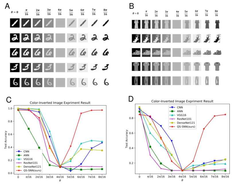
Figure 4: Classification of color-inverted images. (A) MNIST background color-inverted images. Parameter $\theta$ takes values from 0 to $\frac{\pi}{2}$, denoting the degree of color inversion. (B) Fashion-MNIST background-color-inverted images. (C) Background color-inverted MNIST classification results. QS-SNN initially showed performance degeneration similar to that of the fully connected ANN and CNN, with $\theta$ values from 0 to $\frac{4\pi}{16}$. However, as the background-inversion degree further increased, QS-SNN gradually recovered its accuracy, whereas the other networks did not. When the background was totally inverted ($\theta=\frac{8\pi}{16}$), QS-SNN showed almost the same performance as when classifying original images, whereas the second-best network (VGG16) retained only half its original accuracy. (D) Background color-inverted Fashion-MNIST results. Similar results as in the MNIST experiment were achieved, with QS-SNN showing an even greater advantage (right-hand side).

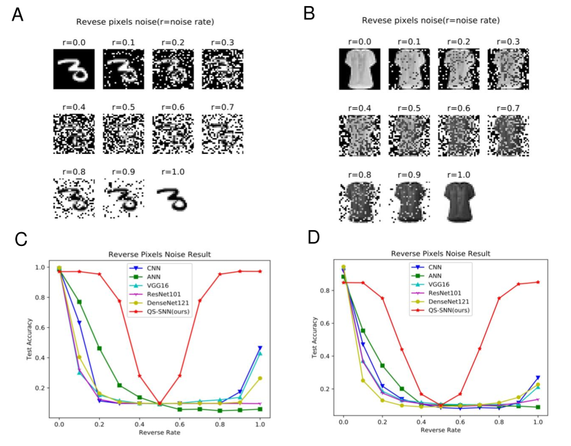
Figure 5: Reverse spike noise results. (A) Reverse spike noise MNIST. The possibility of pixel inversion is controlled by parameter $r$. When $r=0$, no noise is added, i.e., the image is original data. When $r=1.0$, all pixels are flipped. (B) Reverse spike noise Fashion-MNIST. (C) Classification of MNIST images with reverse noise. QS-SNN performed better compared with the inverted background experiment. (D) Classification of Fashion-MNIST images with reverse noise.

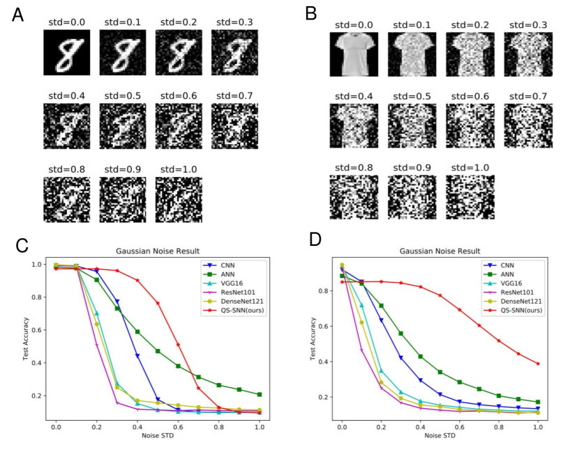
Figure 6: Gaussian noise image classification. (A) Additive white Gaussian noise on MNIST. The mean of Gaussian random noise was set to zero, and different $std$ values were used. (B) Additive white Gaussian noise on Fashion-MNIST. (C) Classification of MNIST images with Gaussian noise. Compared with other networks, QS-SNN showed much slower degeneration. (D) Classification of Fashion-MNIST images with Gaussian noise. QS-SNN performed even better compared with its results on MNIST.

DISCUSSION

This work aimed to integrate quantum theory with a biologically plausible SNN. Quantum image encoding and quantum superposition states were used for information representation, followed by processing with a spatial-temporal SNN. A time-convolution synapse was built to obtain neuron process phase information, and dendrite prediction with a proximal gradient method was used to train the QS-SNN. The proposed QS-SNN showed good performance on color-inverted image recognition tasks that were very challenging to other models. Compared with traditional ANN models, QS-SNN showed better generalization ability.

It is worth noting that the quantum brain hypothesis is quite controversial. Nevertheless, this paper does not aim to provide direct persuasive evidence for the quantum brain hypothesis but to explore novel information processing methods inspired by quantum information theory and brain spiking signal transmission.

Limitations of the study

Our model was inspired by quantum image processing methods, in particular, quantum image superposition state presentation. The model and corresponding experiments were run on a classical computer and did not use any quantum hardware; thus, our work could not benefit from quantum computing. Artificial neurons can be reformed to run on quantum computers [Schuld et al., 2014, Cao et al., 2017, Mangini et al., 2020]. Efforts to build a quantum spiking neuron are still at a preliminary stage [Kristensen et al., 2019]. Simulating spiking neuronal networks on a classical computer is hindered by heavy resource consumption and slow processing.

Future work includes modifying both the quantum superposition encoding strategy and the SNN architecture to suit quantum computing better. In computational neuroscience research, neuronal spikes are typically generated with the Poisson process, which samples data from the binomial distribution. Quantum bits, also named qubits, are fundamental components in a quantum computer. A qubit can take the value of ”0” or ”1” with a certain probability, which is very similar to neuronal spikes. Thus, a set of qubits can encode all possible states of a spike train, as well as the quantum superposition images, in the quantum computer. Although it requires much effort to reconstruct spiking neural models suited for quantum computing, it is significant in neurology and artificial intelligence research to explore more quantum-inspired mechanisms to explain brain functions that traditional theories fail to.

Method details

Generating background inverse image

Different degree of background color inverse images $\mathinner{|I(\Theta)\rangle}$ using for experiment are generated according to the quantum superposition encoding. Here we describe the numerical form value of quantum image used to test model. Suppose the original image is represented by $X$ and the reversed image is $\bar{X}$. Parameter $\Theta$ controls the proportion of original image and reverse image in background color inverse images with

$$I(\Theta)=Xcos(\Theta)+\bar{X}sin(\Theta)$$ (20)

Learning procedure of the QS-SNN algorithm

Dendrite prediction [Urbanczik and Senn, 2014] and proximal gradient methods are used for tuning of QS-SNN. In Equation (21), $I_{i}$ is the teaching current, which is the integration of correct labels in $g_{E_{i}}(E_{E}-U_{1})$ and wrong labels in $g_{I_{i}}(E_{I}-U_{1})$. $E_{E}$ (8 mV) and $E_{I}$ (-8 mV) are the excitatory and inhibitory standard membrane potentials, respectively. The teaching current is injected to the soma of neurons in the output layer, generating added potential $V_{I_{i}}$ with membrane resistance $r_{B}$, as shown in Equation (22):

$$\left\{\begin{array}[]{l}I^{ject}_{i}=g_{E_{i}}(E_{E}-U_{1})+g_{I_{i}}(E_{I}-U_{1})\\ g_{E_{i}}=\left\{\begin{array}[]{lr}1,\quad i=label,\\ 0,\quad i\neq label.\end{array}\right.\\ g_{I_{i}}=\left\{\begin{array}[]{lr}0,\quad i=label,\\ 1,\quad i\neq label.\end{array}\right.\\ V_{I_{i}}=r_{B}\cdot I^{ject}_{i},\end{array}\right.$$ (21)

$$\tau_{L}\frac{dV_{i}^{o}(t)}{dt}=-V_{i}^{o}(t)+\frac{g_{B}}{g_{L}}(V_{i}^{o,b}-V_{i}^{o}(t))+V_{I_{i}}-V_{i}^{o}(t).$$ (22)

Setting the left side of Equation (22) to zero and $V_{i}^{o}=V_{I_{i}}$, we get the steady state of somatic potentials $V_{i}^{o}$ and $V_{i}^{o,b}$ with $V_{i}^{o*}=g_{B}/(g_{B}+g_{L})V_{i}^{o,b}$. The dendrite prediction rule defines the soma-dendrite error as Equation (23):

$$L=\frac{1}{2}\sum\limits_{i=0}^{N}\parallel r_{max}\sigma(V_{i}^{o})-r_{max}\sigma(V_{i}^{o*})\parallel^{2}.$$ (23)

Minimizing this error based on the differential chain rule, we obtain updated synaptic weights $w_{ij}^{o}$, as shown in Equations (24) and (25):

$$\frac{\partial L}{\partial w_{ij}^{o}} =\frac{\partial L}{\partial V_{i}^{o,b}}\frac{\partial V_{i}^{o,b}}{\partial w_{ij}^{o}}$$ (24)

$$=r_{max}\frac{g_{B}}{g_{B}+g_{L}}\left[\sigma(V_{i}^{o*})-\sigma(V_{i}^{o})\right]\sigma^{\prime}(V_{i}^{o*})r_{j}$$

$$=\delta^{o}_{i}r_{j},$$

$$\frac{\partial L}{\partial b_{o}^{1}} =\frac{\partial L}{\partial V_{i}^{o,b}}\frac{\partial V_{i}^{o,b}}{\partial b_{i}^{o}}$$ (25)

$$=r_{max}\frac{g_{B}}{g_{B}+g_{L}}\left[\sigma(V_{i}^{o*})-\sigma(V_{i}^{o})\right]\sigma^{\prime}(V_{i}^{o*})$$

$$=\delta^{o}_{i}.$$

Equation (26) shows the iterative updating of synaptic weights $w_{ij}^{y}$ and bias $b_{i}^{y}$:

$$\left\{\begin{array}[]{l}w_{ij}^{o}\leftarrow w_{ij}^{o}-\eta\frac{\partial L}{\partial w_{ij}^{o}}\\ b_{i}^{o}\leftarrow b_{i}^{o}-\eta\frac{\partial L}{\partial b_{i}^{o}}.\end{array}\right.$$ (26)

For the hidden layer, error signal $\delta_{i}$ is passed from the previous layer, and neuron synapses $w_{ij}^{h}$ are adapted using Equations (27) and (28):

$$\frac{\partial L}{\partial w_{ij}^{h}} =\sum\limits_{k}\frac{\partial L}{\partial V_{k}^{o,b}}\frac{\partial V_{k}^{o,b}}{\partial r_{i}^{h}}\frac{\partial r_{i}^{h}}{\partial V_{i}^{h}}\frac{\partial V_{i}^{h}}{\partial V_{i}^{h,b}}\frac{\partial V_{i}^{h,b}}{\partial w_{ij}^{h}}$$ (27)

$$=\sum\limits_{k}\delta^{o}_{k}w_{ki}^{o}r_{max}\frac{g_{B}}{g_{B}+g_{L}}\sigma^{\prime}(V_{i}^{h})V_{j}^{PSP}$$

$$=\sum\limits_{k}\delta^{o}_{k}\delta^{h}_{i}w_{ki}^{o}V_{j}^{PSP},$$

$$\frac{\partial L}{\partial b_{i}^{h}} =\sum\limits_{k}\frac{\partial L}{\partial V_{k}^{o,b}}\frac{\partial V_{k}^{o,b}}{\partial r_{i}^{h}}\frac{\partial r_{i}^{h}}{\partial V_{i}^{h}}\frac{\partial V_{i}^{h}}{\partial V_{i}^{h,b}}\frac{\partial V_{i}^{h,b}}{\partial b_{i}^{h}}$$ (28)

$$=\sum\limits_{k}\delta^{o}_{k}w_{ki}^{o}r_{max}\frac{g_{B}}{g_{B}+g_{L}}\sigma^{\prime}(V_{i}^{h})$$

$$=\sum\limits_{k}\delta^{o}_{k}\delta^{h}_{i}w_{ki}^{o}.$$

Equation (29) shows the iterative updating of synaptic weights $w_{ij}^{h}$ and bias $b_{i}^{h}$:

$$\left\{\begin{array}[]{l}w_{ij}^{h}\leftarrow w_{ij}^{h}-\eta\frac{\partial L}{\partial w_{ij}^{h}}\\ b_{i}^{h}\leftarrow b_{i}^{h}-\eta\frac{\partial L}{\partial b_{i}^{h}}.\end{array}\right.$$ (29)

The training and test procedure for the QS-SNN model is shown in Algorithm 1.

Algorithm 1 The learning procedure of QS-SNN.

1. Initialize weights $W_{j,i}$ with random uniform distribution, membrane potential states $V_{i}$, and other

 related hyperparameters as in Table S1.

2. Start training procedure with only original images in training dataset, $\theta_{i}=0$:

     2.1 Load training samples.

     2.2 Construct quantum superposition state representations of images.

     2.3 Input neuron spikes as Poisson process with spiking rate and phase time according to quantum

  superposition image.

     2.4 Process time-differential convolution to obtain dynamical updating of membrane potential of

  post-synaptic neurons.

     2.5 Update multi-layer membrane potential.

     2.6 Train the QS-SNN with dendrite prediction and proximal gradient.

     2.7 Select neurons in output layer with maximum spiking rate as the output class.

3. Start test procedure using color-inverse images with different degree of color inversion from the test

  dataset, $\theta_{i}=0,\frac{\pi}{16},\dots,\frac{8\pi}{16}$.

     3.1 Load the test samples and transfer to spike trains as in steps 2.2 and 2.3.

     3.2 Test the performance of the trained QS-SNN on color-inverse images.

     3.3 Output the test performance.

Table T1: Hyperparameters of QS-SNN, Related to STAR Methods

Parameter	Value	Parameter	Value
$\tau$	4.0	$r_{max}$	250 Hz
$\tau_{L}$	10.0 ms	$T$	50 ms
$g_{B}$	0.6 nS	$T_{sp}$	20 ms
$g_{L}$	0.05 nS	$r_{B}$	1.0 n$\Omega$

Table T2: MNIST color-inverted results (accuracy percentages divided by 100), Related to Figure 4

Algorithm	ANN	CNN	VGG16	ResNet101	DenseNet121	QS-SNN
Structure	784-500-10	784-c3p1c3p2c3-256-128-10	-	-	-	784-500-10
$\theta=0$	0.978	0.992	0.996	0.996	0.997	0.971
$\theta=\frac{\pi}{16}$	0.685	0.977	0.996	0.994	0.995	0.972
$\theta=\frac{2\pi}{16}$	0.393	0.942	0.989	0.871	0.974	0.854
$\theta=\frac{3\pi}{16}$	0.124	0.558	0.649	0.194	0.388	0.416
$\theta=\frac{4\pi}{16}$	0.097	0.114	0.114	0.098	0.114	0.089
$\theta=\frac{5\pi}{16}$	0.062	0.031	0.189	0.099	0.218	0.416
$\theta=\frac{6\pi}{16}$	0.054	0.138	0.458	0.103	0.372	0.923
$\theta=\frac{7\pi}{16}$	0.059	0.381	0.504	0.102	0.362	0.970
$\theta=\frac{8\pi}{16}$	0.062	0.469	0.488	0.099	0.350	0.973

Table T3: Fashion-MNIST color-inverted results (accuracy percentages divided by 100), Related to Figure 4.

Algorithm	ANN	CNN	VGG16	ResNet101	DenseNet121	QS-SNN
Structure	784-500-10	784-c3p1c3p2c3-256-128-10	-	-	-	784-500-10
$\theta=0$	0.887	0.918	0.941	0.926	0.946	0.847
$\theta=\frac{\pi}{16}$	0.417	0.812	0.602	0.304	0.718	0.826
$\theta=\frac{2\pi}{16}$	0.194	0.693	0.437	0.126	0.524	0.539
$\theta=\frac{3\pi}{16}$	0.100	0.494	0.308	0.101	0.311	0.224
$\theta=\frac{4\pi}{16}$	0.100	0.100	0.100	0.100	0.100	0.100
$\theta=\frac{5\pi}{16}$	0.100	0.131	0.169	0.100	0.130	0.224
$\theta=\frac{6\pi}{16}$	0.100	0.193	0.177	0.102	0.167	0.656
$\theta=\frac{7\pi}{16}$	0.100	0.229	0.185	0.108	0.203	0.827
$\theta=\frac{8\pi}{16}$	0.098	0.244	0.190	0.120	0.249	0.847

Table T4: MNIST reverse-pixels noise results (accuracy percentages divided by 100), Related to Figure 5.

Algorithm	ANN	CNN	VGG16	ResNet101	DenseNet121	QS-SNN
Structure	784-500-10	784-c3p1c3p2c3-256-128-10	-	-	-	784-500-10
$r=0$	0.985	0.991	0.996	0.996	0.997	0.971
$r=0.1$	0.77	0.631	0.301	0.320	0.404	0.971
$r=0.2$	0.462	0.114	0.153	0.124	0.163	0.954
$r=0.3$	0.217	0.097	0.116	0.098	0.106	0.775
$r=0.4$	0.137	0.097	0.098	0.098	0.099	0.280
$r=0.5$	0.092	0.097	0.094	0.097	0.097	0.095
$r=0.6$	0.057	0.097	0.099	0.097	0.098	0.281
$r=0.7$	0.059	0.097	0.112	0.097	0.098	0.778
$r=0.8$	0.049	0.098	0.121	0.097	0.098	0.953
$r=0.9$	0.053	0.174	0.138	0.097	0.104	0.972
$r=1.0$	0.059	0.464	0.429	0.096	0.264	0.972

Table T5: Fashion-MNIST reverse-pixel noise results (accuracy percentages divided by 100), Related to Figure 5.

Algorithm	ANN	CNN	VGG16	ResNet101	DenseNet121	QS-SNN
Structure	784-500-10	784-c3p1c3p2c3-256-128-10	-	-	-	784-500-10
$r=0$	0.884	0.920	0.94	0.927	0.945	0.848
$r=0.1$	0.555	0.471	0.371	0.366	0.251	0.847
$r=0.2$	0.342	0.217	0.186	0.175	0.130	0.752
$r=0.3$	0.201	0.138	0.132	0.127	0.099	0.441
$r=0.4$	0.108	0.107	0.118	0.110	0.091	0.169
$r=0.5$	0.101	0.086	0.107	0.096	0.092	0.100
$r=0.6$	0.100	0.081	0.105	0.094	0.097	0.169
$r=0.7$	0.099	0.086	0.104	0.099	0.103	0.445
$r=0.8$	0.096	0.083	0.106	0.100	0.116	0.752
$r=0.9$	0.095	0.115	0.108	0.115	0.149	0.839
$r=1.0$	0.089	0.268	0.212	0.136	0.227	0.850

Table T6: MNIST Gaussian noise results (accuracy percentages divided by 100), Related to Figure 6.

Algorithm	ANN	CNN	VGG16	ResNet101	DenseNet121	QS-SNN
Structure	784-500-10	784-c3p1c3p2c3-256-128-10	-	-	-	784-500-10
$std=0$	0.983	0.992	0.996	0.995	0.997	0.972
$std=0.1$	0.976	0.989	0.992	0.986	0.990	0.972
$std=0.2$	0.905	0.956	0.702	0.507	0.635	0.972
$std=0.3$	0.731	0.773	0.275	0.156	0.250	0.961
$std=0.4$	0.589	0.441	0.152	0.117	0.156	0.902
$std=0.5$	0.471	0.176	0.113	0.113	0.142	0.763
$std=0.6$	0.380	0.113	0.103	0.109	0.130	0.510
$std=0.7$	0.313	0.100	0.101	0.113	0.124	0.245
$std=0.8$	0.264	0.098	0.099	0.108	0.116	0.128
$std=0.9$	0.237	0.098	0.099	0.108	0.116	0.100
$std=1.0$	0.207	0.097	0.098	0.107	0.113	0.095

Table T7: Fashion-MNIST Gaussian noise results (accuracy percentages divided by 100), Related to Figure 6.

Algorithm	ANN	CNN	VGG16	ResNet101	DenseNet121	QS-SNN
Structure	784-500-10	784-c3p1c3p2c3-256-128-10	-	-	-	784-500-10
$std=0$	0.884	0.920	0.938	0.934	0.947	0.850
$std=0.1$	0.841	0.851	0.719	0.464	0.621	0.851
$std=0.2$	0.716	0.633	0.349	0.251	0.283	0.852
$std=0.3$	0.559	0.421	0.228	0.168	0.193	0.845
$std=0.4$	0.429	0.294	0.177	0.137	0.155	0.823
$std=0.5$	0.341	0.214	0.154	0.126	0.146	0.774
$std=0.6$	0.284	0.173	0.142	0.119	0.13	0.692
$std=0.7$	0.245	0.157	0.131	0.121	0.124	0.604
$std=0.8$	0.207	0.147	0.126	0.116	0.118	0.518
$std=0.9$	0.188	0.139	0.121	0.110	0.113	0.444
$std=1.0$	0.172	0.134	0.121	0.114	0.111	0.388

References

- Beer et al. [2020] Beer, K., Bondarenko, D., Farrelly, T., Osborne, T.J., Salzmann, R., Scheiermann, D., Wolf, R., 2020. Training deep quantum neural networks. Nat. Commun. 11, 1–6.
- Cao et al. [2017] Cao, Y., Guerreschi, G.G., Aspuru-Guzik, A., 2017. Quantum neuron: an elementary building block for machine learning on quantum computers. arXiv:1711.11240 .
- Cox and Witten [2019] Cox, J., Witten, I.B., 2019. Striatal circuits for reward learning and decision-making. Nat. Rev. Neurosci. 20, 482–494.
- Dan and Poo [2004] Dan, Y., Poo, M.M., 2004. Spike timing-dependent plasticity of neural circuits. Neuron 44, 23–30.
- Dendukuri and Luu [2018] Dendukuri, A., Luu, K., 2018. Image processing in quantum computers. arXiv preprint arXiv:1812.11042 .
- Fisher [2015] Fisher, M.P., 2015. Quantum cognition: the possibility of processing with nuclear spins in the brain. Ann. Phys. 362, 593–602.
- Frémaux and Gerstner [2016] Frémaux, N., Gerstner, W., 2016. Neuromodulated spike-timing-dependent plasticity, and theory of three-factor learning rules. Front. Neural Circuits 9, 85.
- Gerstner [2001] Gerstner, W., 2001. A framework for spiking neuron models: the spike response model, in: Handbook of Biological Physics. Elsevier. volume 4, pp. 469–516.
- Gerstner and Kistler [2002] Gerstner, W., Kistler, W.M., 2002. Spiking neuron models: single neurons, populations, plasticity. Cambridge University Press.
- Grover [1996] Grover, L.K., 1996. A fast quantum mechanical algorithm for database search, in: Proceedings of the Twenty-eighth Annual ACM Symposium on Theory of Computing, ACM. pp. 212–219.
- Harrow et al. [2009] Harrow, A.W., Hassidim, A., Lloyd, S., 2009. Quantum algorithm for linear systems of equations. Phys. Rev. Lett. 103, 150502.
- He et al. [2016] He, K., Zhang, X., Ren, S., Sun, J., 2016. Deep residual learning for image recognition. Proceedings of the IEEE conference on computer vision and pattern recognition , 770–778.
- Héricé et al. [2016] Héricé, C., Khalil, R., Moftah, M., Boraud, T., Guthrie, M., Garenne, A., 2016. Decision making under uncertainty in a spiking neural network model of the basal ganglia. J. Integr. Neurosci. 15, 515–538.
- Huang et al. [2017] Huang, G., Liu, Z., Van Der Maaten, L., Weinberger, K.Q., 2017. Densely connected convolutional networks. Proceedings of the IEEE conference on computer vision and pattern recognition , 4700–4708.
- Iyengar et al. [2020] Iyengar, S.S., Kumar, L.K., Mastriani, M., 2020. Analysis of five techniques for the internal representation of a digital image inside a quantum processor. arXiv preprint arXiv:2008.01081 .
- Izhikevich [2003] Izhikevich, E.M., 2003. Simple model of spiking neurons. IEEE Trans. Neural Netw. 14, 1569–1572.
- Khalil et al. [2017] Khalil, R., Moftah, M.Z., Moustafa, A.A., 2017. The effects of dynamical synapses on firing rate activity: a spiking neural network model. Eur. J. Neurosci. 46, 2445–2470.
- Kristensen et al. [2019] Kristensen, L.B., Degroote, M., Wittek, P., Aspuru-Guzik, A., Zinner, N.T., 2019. An artificial spiking quantum neuron. arXiv:1907.06269.
- Le et al. [2011] Le, P.Q., Dong, F., Hirota, K., 2011. A flexible representation of quantum images for polynomial preparation, image compression, and processing operations. Quantum Inf. Process. 10, 63--84.
- Lecun et al. [1998] Lecun, Y., Bottou, L., Bengio, Y., Haffner, P., 1998. Gradient-based learning applied to document recognition. Proceedings of the IEEE 86, 2278--2324. doi:10.1109/5.726791.
- LeCun et al. [2010] LeCun, Y., Cortes, C., Burges, C., 2010. MNIST handwritten digit database. ATT Labs. http://yann.lecun.com/exdb/mnist .
- Lloyd et al. [2014] Lloyd, S., Mohseni, M., Rebentrost, P., 2014. Quantum principal component analysis. Nat. Phys. 10, 631.
- Maass [1997] Maass, W., 1997. Networks of spiking neurons: the third generation of neural network models. Neural Netw. 10, 1659--1671.
- Mangini et al. [2020] Mangini, S., Tacchino, F., Gerace, D., Macchiavello, C., Bajoni, D., 2020. Quantum computing model of an artificial neuron with continuously valued input data. Mach. Learn. Sci. Technol. 1, 045008.
- Manju and Nigam [2014] Manju, A., Nigam, M.J., 2014. Applications of quantum inspired computational intelligence: a survey. Artif. Intell. Rev. 42, 79--156.
- Mastriani [2020] Mastriani, M., 2020. Quantum image processing: the truth, the whole truth, and nothing but the truth about its problems on internal image representation and outcomes recovering. arXiv preprint arXiv:2002.04394 .
- Schuld et al. [2014] Schuld, M., Sinayskiy, I., Petruccione, F., 2014. The quest for a quantum neural network. Quantum Inf. Process. 13, 2567--2586.
- Schuld et al. [2015] Schuld, M., Sinayskiy, I., Petruccione, F., 2015. Simulating a perceptron on a quantum computer. Phys. Lett. A 379, 660--663.
- Shor [1999] Shor, P.W., 1999. Polynomial-time algorithms for prime factorization and discrete logarithms on a quantum computer. SIAM Rev. 41, 303--332.
- Shrestha and Orchard [2018] Shrestha, S.B., Orchard, G., 2018. SLAYER: spike layer error reassignment in time, in: Advances in Neural Information Processing Systems, pp. 1412--1421.
- Simonyan and Zisserman [2015] Simonyan, K., Zisserman, A., 2015. Very deep convolutional networks for large-scale image recognition. CoRR abs/1409.1556.
- Song et al. [2000] Song, S., Miller, K.D., Abbott, L.F., 2000. Competitive Hebbian learning through spike-timing-dependent synaptic plasticity. Nat. Neurosci. 3, 919.
- Torrontegui and García-Ripoll [2019] Torrontegui, E., García-Ripoll, J.J., 2019. Unitary quantum perceptron as efficient universal approximator. Europhys. Lett. 125, 30004.
- Urbanczik and Senn [2014] Urbanczik, R., Senn, W., 2014. Learning by the dendritic prediction of somatic spiking. Neuron 81, 521--528.
- Vaziri and Plenio [2010] Vaziri, A., Plenio, M.B., 2010. Quantum coherence in ion channels: resonances, transport and verification. New J. Phys. 12, 085001.
- Weingarten et al. [2016] Weingarten, C.P., Doraiswamy, P.M., Fisher, M.P.A., 2016. A new spin on neural processing: Quantum cognition. Front. Human Neurosci. 10, 541.
- Xiao et al. [2017] Xiao, H., Rasul, K., Vollgraf, R., 2017. Fashion-MNIST: a novel image dataset for benchmarking machine learning algorithms. arXiv:cs.LG/1708.07747.
- Xiao et al. [2010] Xiao, J., Yan, Y., Zhang, J., Tang, Y., 2010. A quantum-inspired genetic algorithm for k-means clustering. Exp. Syst. Appl. 37, 4966--4973.
- Zeng et al. [2017] Zeng, Y., Zhang, T., Xu, B., 2017. Improving multi-layer spiking neural networks by incorporating brain-inspired rules. Sci. China Inform. Sci. 60, 052201.
- Zenke et al. [2015] Zenke, F., Agnes, E.J., Gerstner, W., 2015. Diverse synaptic plasticity mechanisms orchestrated to form and retrieve memories in spiking neural networks. Nat. Commun. 6, 6922--6922.
- Zhao et al. [2017] Zhao, F., Zhang, T., Zeng, Y., Xu, B., 2017. Towards a brain-inspired developmental neural network by adaptive synaptic pruning, in: The 24th International Conference on Neural Information Processing, Springer. pp. 182--191.