Empirical Likelihood Inference for Area under the ROC Curve using Ranked Set Samples

Abstract

[Summary]The area under a receiver operating characteristic curve (AUC) is a useful tool to assess the performance of continuous-scale diagnostic tests on binary classification. In this article, we propose an empirical likelihood (EL) method to construct confidence intervals for the AUC from data collected by ranked set sampling (RSS). The proposed EL-based method enables inferences without assumptions required in existing nonparametric methods and takes advantage of the sampling efficiency of RSS. We show that for both balanced and unbalanced RSS, the EL-based point estimate is the Mann-Whitney statistic, and confidence intervals can be obtained from a scaled chi-square distribution. Simulation studies and two case studies on diabetes and chronic kidney disease data suggest that using the proposed method and RSS enables more efficient inference on the AUC.

, , and (), Empirical Likelihood Inference for Area under the ROC Curve using Ranked Set Samples, Pharm. Stat., .

1 Introduction

A receiver operating characteristic (ROC) curve is used to evaluate the performance of a diagnostic test with binary outcomes. Let $X$ and $Y$ denote continuous measurements of non-diseased and diseased subjects with distribution functions $F$ and $G$, respectively. The diagnostic test classifies a subject as having the disease if the measurement is greater than the threshold $c$. The ROC curve plots the sensitivity (the true positive rate, $p=P(Y\geq c)=1-G(c)$) versus $1-$specificity (the false positive rate, $q=1-P(X\leq c)=F(c)$) of the diagnostic test for all possible threshold values. The ROC curve can be expressed as a function $R(p)=1-G(F^{-1}(p))$, for $0\leq p\leq 1$. The area under the ROC curve (AUC), denoted $\delta$, is an effective summary measure of the test’s overall accuracy. Bamber¹ shows that $\delta=P(Y\geq X)$, which can be interpreted as the probability that the measurement of a randomly selected diseased subject is higher than that of a randomly selected non-diseased subject.

Many nonparametric approaches have been widely used to estimate the AUC from simple random samples, including the Mann-Whitney (MW) statistic, the kernel method, and the empirical likelihood (EL) approach. First, the MW statistic is an unbiased estimator of the AUC, and the confidence interval can be obtained using its asymptotic normality ¹, ². However, the normal approximation often requires a large number of samples or leads to low coverage for high values of the AUC in finite samples ³. Second, the kernel method estimates the continuous ROC curve by replacing the indicator function of the empirical cumulative distribution with kernels^{4, 5}. The AUC can be obtained by computing the area under the kernel smoothed ROC curve. The kernel method usually requires optimal bandwidth to minimize the estimation error. Although optimal bandwidth selection is well studied for the estimation of the density itself, it has not been extensively studied for the estimation of the AUC. Lastly, the EL approach for the AUC is proposed by Qin and Zhou³ to build confidence intervals for the MW estimator. EL is a nonparametric method of inference introduced by Owen^{6, 7, 8}. EL enables a distribution-free inference while carrying nice properties of the conventional likelihood such as Wilk’s theorem ⁷ and Bartlett correction ⁹. Regarding the inference on the AUC, Qin and Zhou³ show that their EL approach provides a better interval estimation in view of the coverage probability and the length of the interval.

Ranked set sampling (RSS), firstly proposed by McIntyre¹⁰, is a cost-effective sampling method compared to simple random sampling (SRS). RSS is especially useful when precise measurement of primary outcomes is expensive but assessment of their relative ranks is feasible. Various topics have been studied on RSS such as distribution functions ¹¹, nonparametric two-sample tests ¹², ¹³, and rank regression ¹⁴. In the past decade, RSS has been applied to diverse areas including agriculture¹⁵, ¹⁶, ¹⁷, ¹⁸, ¹⁹, education²⁰, engineering²¹, environment²², ²³, public health²⁴, ²⁵, ²⁶, ²⁷, ²⁸, and medicine²⁹, ²⁷.

The main theme of this paper is the inference on the AUC based on EL when data are obtained from RSS. In RSS, the estimation and testing of the AUC have been of great interest. Bohn and Wolfe^{12, 13} show the asymptotic normality of the MW statistic of RSS under the location shift distributional assumption $G(x)=F(x-\Delta)$, where $-\infty<\Delta<\infty$. Sengupta and Mukhuti³⁰ show the efficiency of the MW statistic of RSS over SRS. The kernel methods for RSS also have been introduced ^{31, 32}. On the other hand, the EL approach for estimating AUC in RSS has not been much studied. Only a few EL methods have been proposed for some specific topics in RSS³³, ³⁴, ³⁵. First, Baklizi^{34, 35} proposes EL methods to construct confidence intervals for population mean and quantiles from one-sample (balanced and unbalanced) RSS data. Thus, these methods cannot be applied to AUC inferences involving two populations. Second, Liu et al.³³ study EL-based hypothesis testing and interval estimation for one- and two-sample RSS data that mainly focus on mean and mean difference, with extension to general estimating equations. However, their approach is only developed for BRSS. It also does not take full advantage of information obtained from RSS as it assigns equal weight to all measured units in the same cycle of BRSS. To overcome these limitations, we propose EL-based methods for the AUC interval estimation that may better utilize the information obtained from balanced and unbalanced ranked set samples. Like other EL-based methods, our method does not make any distributional assumptions and does not have an additional parameter to be tuned, such as bandwidth. We illustrate the performance of the proposed EL-method via simulation using purely synthetic data and data re-sampled from two case studies, one involving diabetes data and the other involving chronic kidney disease data.

The rest of the paper is organized as follows. In Section 2, we introduce RSS and basic notations needed for our study, and propose the EL methods to estimate the AUC for balanced and unbalanced RSS. In Section 3, we conduct simulation studies under various settings to compare the performance of the proposed EL-based methods for RSS with the existing EL-based method for SRS and kernel-based method for RSS. In Section 4, we apply the proposed method to two case studies of diabetes and chronic kidney disease data and compare it with the other known methods. Discussion and conclusion are given in Section 5.

2 Methods

2.1 Ranked Set Sampling

Let $Y$ be the variable of interest. The RSS scheme can be described as follows. First, the SRS sample of size $n$ is generated from the population of $Y$. Then the $n$ sample units are ranked by judgment without actually measuring $Y$. If there is an easily available concomitant variable, then it can be used to rank the units approximately. From the $n$ ranked sample units, the $r$th smallest one is chosen for actual quantification and is denoted $Y_{[r]1}$; all the other $n-1$ units are discarded. Note that this single RSS observation is obtained using auxiliary ranking information from the $n-1$ observations that are only used for ranking. This procedure continues until $l_{r}$ observations $\{Y_{[r]1},Y_{[r]2},\ldots,Y_{[r]l_{r}}\}$, all with rank $r$, are obtained and the set of these observations is called the $r$th rank stratum. The similar process is repeated for $r=1,\ldots,n$ so that $n$ strata are obtained. The ranked set sample of $Y$ can be represented as

$$Y_{[1]1},Y_{[1]2},\cdots Y_{[1]l_{1}}$$

$$Y_{[2]1},Y_{[2]2},\cdots Y_{[2]l_{2}}$$

$$\cdots\;\;\;\cdots\;\;\;\cdots\;\;\;\cdots$$

$$Y_{[n]1},Y_{[n]2}\cdots Y_{[n]l_{n}},$$

where the $r$th row is the $r$th rank stratum. As a result, it takes $n\sum_{r=1}^{n}l_{r}$ number of sample units to obtain $\sum_{r=1}^{n}l_{r}$ number of RSS observations. In the above RSS sample, $n$ is referred to as the set size and the total sample size is the total number of units formally quantified, given by $\sum_{r=1}^{n}l_{r}$.

In balanced RSS (BRSS), the same number of sample units is assigned to all $n$ strata $(l=l_{1}=l_{2}=\ldots=l_{n})$, where the $s$th column $\{Y_{[1]s},Y_{[2]s},\ldots,Y_{[n]s}\}$ is called the $s$th cycle with set size $n$. On the other hand, unbalanced RSS (URSS) quantifies different number of observations in each rank stratum so that at least one $l_{r}$ is not equal to the others.

RSS provides more efficient inference compared to SRS. For example, let $\{Y_{[1]},Y_{[2]},\ldots,Y_{[n]}\}$ be the BRSS samples of size $n$ from a single cycle and $\{Y_{1},Y_{2},\ldots,Y_{n}\}$ be the SRS samples of size $n$. The BRSS and SRS estimators for population mean are $\overline{Y}_{BRSS}=\frac{1}{n}\sum_{i=1}^{n}Y_{[i]}$ and $\overline{Y}_{SRS}=\frac{1}{n}\sum_{i=1}^{n}Y_{i}$, respectively. Both estimators are unbiased $E[Y]=E\left[\overline{Y}_{BRSS}\right]=E\left[\overline{Y}_{SRS}\right]$, but the variance of the BRSS estimator is always smaller than or equal to that of the SRS estimator $\text{Var}\left(\overline{Y}_{BRSS}\right)\leq\text{Var}\left(\overline{Y}_{SRS}\right)$ ^{36, 37}.

RSS can improve the efficiency of comparisons regardless of the set size. The set size and the ranking quality play an important role in determining sampling efficiency in RSS. In practice, small set sizes are preferred because ranking a large number of units by judgment may be difficult and there is no way to guarantee the ranking quality. In our numerical study, we use small set sizes in the set $\{2,4,5\}$.

2.2 Empirical Likelihood Method for AUC with Balanced RSS

Let samples of $X$ and $Y$ be obtained by BRSS. Also, let $Y_{[r]s}$ be the observation of a diseased subject in the $r$th sample of the $s$th cycle, which is judged to be the $r$th smallest. We assume that the diseased observations are obtained from $l>1$ cycles, each containing $n$ quantified units with ranks from $1$ to $n$, so that $r=1,\ldots,n$ and $s=1,\ldots,l$. Similarly, the non-diseased observations $X_{[i]j}$’s are obtained by BRSS of $k>1$ cycles with size $m$, $i=1,\ldots,m$ and $j=1,\ldots,k$.

Let us write

$$\phi(X_{[i]j},Y_{[r]s})=\left\{\begin{array}[]{@{}ll@{}}1,&\text{if}\ X_{[i]j}<Y_{[r]s}\\ 0,&\text{otherwise.}\end{array}\right.$$

The MW statistic of the AUC based on BRSS is

$$\widehat{\delta}_{BRSS} = U_{BRSS}\left(Y_{[1]1},\ldots,Y_{[1]l},\ldots,Y_{[n]1},\ldots,Y_{[n]l};X_{[1]1},\ldots,X_{[1]k},\ldots,X_{[m]1},\ldots,X_{[m]k}\right)$$

$$= \frac{1}{mknl}\sum\limits_{i=1}^{m}\sum\limits_{j=1}^{k}\sum\limits_{r=1}^{n}\sum\limits_{s=1}^{l}\phi(X_{[i]j},Y_{[r]s}).$$

We can define the placement value of $Y_{[r]s}$ similar to Pepe and Cai³⁸ as

$$U_{rs}=1-F(Y_{[r]s}).$$

Here, $U_{rs}$ can be seen as a proportion of non-diseased subjects whose measurements are greater than $Y_{[r]s}$. By treating $Y_{[r]s}$’s as independent and identically distributed (i.i.d.) random variables from the distribution function $G(\cdot)$, the AUC ($\delta$) can be obtained by using $U_{rs}$,

$$E\left[\sum\limits_{r=1}^{n}\sum\limits_{s=1}^{l}\frac{1}{nl}\left(1-U_{rs}\right)\right]=E[F(Y)]=\delta.$$ (1)

Here, the stratification is not considered by treating the RSS data as if they were i.i.d. However, this has often been a beneficial approach in BRSS³⁴.

We can derive an EL procedure using the relationship between $U_{rs}$ and $\delta$ given in (1). Let $\mathbf{p}=\left(p_{11},\ldots,p_{rs},\ldots,p_{nl}\right)$ be a probability vector such that $\sum_{r=1}^{n}\sum_{s=1}^{l}p_{rs}=1$ and $p_{rs}\geq 0$ for all $r=1,\ldots,n$ and $s=1,\ldots,l$. The profile EL for the AUC using balanced ranked set samples evaluated at the true AUC value $\delta_{0}$ is

$$L_{BRSS}(\delta_{0})=\sup\left\{\prod\limits_{r=1}^{n}\prod\limits_{s=1}^{l}p_{rs}:\sum\limits_{r=1}^{n}\sum\limits_{s=1}^{l}p_{rs}=1,\sum\limits_{r=1}^{n}\sum\limits_{s=1}^{l}p_{rs}\left(1-U_{rs}-\delta_{0}\right)=0\right\}.$$ (2)

Because $U_{rs}$ depends on the unknown non-disease population distribution function $F$, following Qin and Zhou³, we estimate it using the empirical distribution of $\widehat{F}$ as defined in Stokes and Sager¹¹. By replacing $U_{rs}$ with $\widehat{U}_{rs}=1-\widehat{F}\left(Y_{[r]s}\right)=1-\frac{1}{mk}\sum\limits_{i=1}^{m}\sum\limits_{j=1}^{k}\phi\left(X_{[i]j},Y_{[r]s}\right)$ in (2) and solving the Lagrange multiplier, we get

$$p_{rs}=\frac{1}{nl}\left(1+\lambda\left(1-\widehat{U}_{rs}-\delta_{0}\right)\right)^{-1},$$

where $\lambda$ is the solution to

$$0=\frac{1}{nl}\sum\limits_{r=1}^{n}\sum\limits_{s=1}^{l}\frac{\left(1-\widehat{U}_{rs}-\delta_{0}\right)}{1+\lambda\left(1-\widehat{U}_{rs}-\delta_{0}\right)}.$$ (3)

The empirical log-likelihood ratio is

$$l_{BRSS}(\delta_{0})=2\sum\limits_{r=1}^{n}\sum\limits_{s=1}^{l}\log\left(1+\lambda\left(1-\widehat{U}_{rs}-\delta_{0}\right)\right).$$ (4)

The maximum empirical likelihood estimator (MELE) $\tilde{\delta}_{BRSS}$ can be obtained by

$$\tilde{\delta}_{BRSS}=\operatorname*{argmin}_{\delta}l_{BRSS}(\delta).$$

In our setting, $\tilde{\delta}_{BRSS}=\widehat{\delta}_{BRSS}$ because the dimension of $\delta$ and the constraint is the same and $\widehat{\delta}_{BRSS}$ is the solution of $\sum\limits_{r=1}^{n}\sum\limits_{s=1}^{l}\left(1-\widehat{U}_{rs}-\delta\right)=0$ ³⁹.

The standard EL theory cannot be applied to equation (4) because $\widehat{U}_{rs}$ are not independent. Instead, we study the limiting distribution of the scaled EL ⁴⁰, ⁴¹, ⁴². The following theorem shows that the asymptotic distribution of $l_{BRSS}(\delta_{0})$ follows the scaled chi-square distribution with one degree of freedom. The proof is given in Appendix A.

Theorem 2.1.

Assume that rankings of BRSS are consistent and the true value of the AUC is $\delta_{0}$. For fixed $m$ and $n$ as $k\rightarrow\infty$ and $l\rightarrow\infty$,

$$r_{BRSS}(\delta_{0})l_{BRSS}(\delta_{0})\rightarrow\chi^{2}_{1},$$

where

$$r_{BRSS}(\delta_{0}) = \frac{mk}{mk+nl}\frac{\sum\limits_{r=1}^{n}\sum\limits_{s=1}^{l}\frac{1}{nl}\left(1-\widehat{U}_{rs}-\delta_{0}\right)^{2}}{S_{BRSS}^{2}},$$

$$S_{BRSS}^{2} = \frac{nl\left(S_{BRSS}^{10}\right)^{2}+mk\left(S_{BRSS}^{01}\right)^{2}}{mk+nl},$$

$$\left(S_{BRSS}^{10}\right)^{2} = \sum\limits_{i=1}^{m}\sum\limits_{j=1}^{k}\frac{1}{m(k-1)}\left(V_{BRSS}^{10}(X_{[i]j})-\overline{V}^{10}_{BRSS[i]}\right)^{2},$$

$$\left(S_{BRSS}^{01}\right)^{2} = \sum\limits_{r=1}^{n}\sum\limits_{s=1}^{l}\frac{1}{n(l-1)}\left(V_{BRSS}^{01}(Y_{[r]s})-\overline{V}^{01}_{BRSS[r]}\right)^{2},$$

$V_{BRSS}^{10}(X_{[i]j})=\frac{1}{nl}\sum\limits_{r=1}^{n}\sum\limits_{s=1}^{l}\phi(X_{[i]j},Y_{[r]s})$, $V_{BRSS}^{01}(Y_{[r]s})=\frac{1}{mk}\sum\limits_{i=1}^{m}\sum\limits_{j=1}^{k}\phi(X_{[i]j},Y_{[r]s})$,

$\overline{V}_{BRSS[i]}^{10}=\frac{1}{k}\sum\limits_{j=1}^{k}V_{BRSS}^{10}(X_{[i]j})$, and $\overline{V}_{BRSS[r]}^{01}=\frac{1}{l}\sum\limits_{s=1}^{l}V_{BRSS}^{01}(Y_{[r]s})$.

We can use Theorem 2.1 to find an interval estimate for $\delta$. An EL $100(1-\alpha)\%$ confidence interval for the AUC based on BRSS samples can be found as

$$CI_{\alpha}(\delta)=\left\{\delta:r_{BRSS}(\delta)l_{BRSS}(\delta)\leq\chi_{1,1-\alpha}^{2}\right\},$$ (5)

where $\chi_{1,1-\alpha}^{2}$ is the $(1-\alpha)$ quanatile of $\chi^{2}_{1}$ distribution. By Theorem 2.1, the confidence interval (5) asymptotically achieves the correct coverage probability $1-\alpha$. For simplicity, we approximate $r_{BRSS}(\delta)$ with $r_{BRSS}(\widehat{\delta}_{BRSS})$ in (5).

2.3 Empirical Likelihood Method for AUC with Unbalanced RSS

We extend the proposed EL method to URSS with equal set sizes. In URSS, the number of observations in each rank stratum is not equal. For the measurements of diseased subjects $Y$, the number of observations of the $r$th rank stratum is $l_{r}$ for $r=1,\ldots,n$, and the total number of ranked set samples becomes $n_{y}=\sum\limits_{r=1}^{n}l_{r}$. Similarly, the measurements of non-diseased subjects $X$ are obtained $k_{i}$ times in the rank $i$ stratum for $i=1,\ldots,m$, and the total number of observations is $n_{x}=\sum\limits_{i=1}^{m}k_{i}$. We assume $l_{r}>1$ for $r=1,\ldots,n$ and $k_{i}>1$ for $i=1,\ldots,m$.

The MW statistic of the AUC based on URSS is

$$\widehat{\delta}_{URSS} = U_{URSS}\left(Y_{[1]1},\ldots,Y_{[1]l_{1}},\ldots,Y_{[n]1},\ldots,Y_{[n]l_{n}};X_{[1]1},\ldots,X_{[1]k_{1}},\ldots,X_{[m]1},\ldots,X_{[m]k_{m}}\right)$$

$$= \sum\limits_{i=1}^{m}\sum\limits_{j=1}^{k_{i}}\sum\limits_{r=1}^{n}\sum\limits_{s=1}^{l_{r}}\frac{1}{mk_{i}nl_{r}}\phi(X_{[i]j},Y_{[r]s}).$$

Using the relationship between $U_{rs}$ and the AUC $\delta$ and treating the data as i.i.d., we can show that $E\left[\sum\limits_{r=1}^{n}\sum\limits_{s=1}^{l_{r}}\frac{1}{nl_{r}}\left(1-U_{rs}\right)\right]=\delta$. Let $\mathbf{w}=\left(w_{11},\ldots,w_{1l_{1}},\ldots,w_{rs},\ldots,w_{nl_{n}}\right)$ be a weight vector such that $\sum_{r=1}^{n}\sum_{s=1}^{l}\frac{w_{rs}}{nl_{r}}=1$ where $w_{rs}\geq 0$ for all $r=1,\ldots,n$ and $s=1,\ldots,\max\{l_{1},\ldots,l_{n}\}$. The profile EL for the AUC of URSS evaluated at the true value $\delta_{0}$ can be defined as

$$L_{URSS}(\delta_{0})=\sup\left\{\prod\limits_{r=1}^{n}\prod\limits_{s=1}^{l_{r}}w_{rs}:\sum\limits_{r=1}^{n}\sum\limits_{s=1}^{l_{r}}\frac{w_{rs}}{nl_{r}}=1,\sum\limits_{r=1}^{n}\sum\limits_{s=1}^{l_{r}}\frac{w_{rs}}{nl_{r}}\left(1-U_{rs}-\delta_{0}\right)=0\right\}.$$ (6)

The first constraint in equation (6) implies that $w_{rs}$ is weighted by the number of measurements in the $r$th rank stratum $l_{r}$. By replacing $U_{rs}$ with $\widehat{U}_{rs}=1-\widehat{F}(Y_{[r]s})=1-\sum\limits_{i=1}^{m}\sum\limits_{j=1}^{k_{i}}\frac{1}{mk_{i}}\phi(X_{[i]j},Y_{[r]s})$ and solving (6),

$$w_{rs}=\frac{1}{n_{y}}\left(1+\lambda\frac{1}{nl_{r}}\left(1-\widehat{U}_{rs}-\delta_{0}\right)\right)^{-1}.$$

The empirical log-likelihood ratio becomes

$$l_{URSS}(\delta_{0})=2\sum\limits_{r=1}^{n}\sum\limits_{s=1}^{l_{r}}\log\left(1+\lambda\frac{1}{nl_{r}}\left(1-\widehat{U}_{rs}-\delta_{0}\right)\right).$$ (7)

It can be easily shown that the MELE of (7) $\tilde{\delta}_{URSS}=\widehat{\delta}_{URSS}$ for the same reason explained in Section 2.2.

The proposed EL-based method for BRSS can be easily extended to URSS. Theorem 2.2 shows the asymptotic result of the empirical log-likelihood ratio for URSS. The proof is given in Appendix A. We can obtain an $100(1-\alpha)\%$ EL confidence interval for the AUC with URSS by

$$CI_{\alpha}(\delta)=\left\{\delta:r_{URSS}(\delta)l_{URSS}(\delta)\leq\chi_{1,1-\alpha}^{2}\right\}.$$ (8)

Similarly, we use $r_{URSS}(\widehat{\delta}_{URSS})$ to approximate $r_{URSS}(\delta)$ in (8).

Theorem 2.2.

Assume that rankings of URSS are consistent and the true value of the AUC is $\delta_{0}$. For fixed $m$ and $n$, as $\min\limits_{r}l_{r}\rightarrow\infty$ and $\min\limits_{i}k_{i}\rightarrow\infty$,

$$r_{URSS}(\delta_{0})l_{URSS}(\delta_{0})\rightarrow\chi^{2}_{1},$$

where

$$r_{URSS}(\delta_{0}) = \frac{n_{x}}{n_{y}+n_{x}}\frac{\sum\limits_{r=1}^{n}\sum\limits_{s=1}^{l_{r}}\frac{1}{nl_{r}}\left(1-\widehat{U}_{rs}-\delta_{0}\right)^{2}}{S_{URSS}^{2}},$$

$$S_{URSS}^{2} = \frac{n_{y}\left(S_{URSS}^{10}\right)^{2}+n_{x}\left(S_{URSS}^{01}\right)^{2}}{n_{x}+n_{y}},$$

$$\left(S_{URSS}^{10}\right)^{2} = \sum\limits_{i=1}^{m}\sum\limits_{j=1}^{k_{i}}\frac{1}{m(k_{i}-1)}\left(V_{URSS}^{10}(X_{[i]j})-\overline{V}_{URSS[i]}^{10}\right)^{2},$$

$$\left(S_{URSS}^{01}\right)^{2} = \sum\limits_{r=1}^{n}\sum\limits_{s=1}^{l_{r}}\frac{1}{n(l_{r}-1)}\left(V_{URSS}^{01}(Y_{[r]s})-\overline{V}_{URSS[r]}^{01}\right)^{2},$$

$V_{URSS}^{10}(X_{[i]j})=\sum\limits_{r=1}^{n}\sum\limits_{s=1}^{l_{r}}\frac{1}{nl_{r}}\phi(X_{[i]j},Y_{[r]s})$, $V_{URSS}^{01}(Y_{[r]s})=\sum\limits_{i=1}^{m}\sum\limits_{j=1}^{k_{i}}\frac{1}{mk_{i}}\phi(X_{[i]j},Y_{[r]s})$,

$\overline{V}_{URSS[i]}^{10}=\frac{1}{k_{i}}\sum\limits_{j=1}^{k_{i}}V_{URSS}^{10}(X_{[i]j})$, and $\overline{V}_{URSS[r]}^{01}=\frac{1}{l_{r}}\sum\limits_{s=1}^{l_{r}}V_{URSS}^{01}(Y_{[r]s})$.

3 Simulation Studies

3.1 Balanced RSS

In this section, we compare simulation results of our proposed EL intervals of BRSS (BRSS-EL) to the two existing methods mentioned in the introduction: EL intervals of simple random sampling (SRS-EL) of Qin and Zhou³ and kernel-estimation intervals of BRSS (BRSS-KER) of Yin et al.³². We use SRS-EL as a reference simple random sampling method because it outperforms the other SRS-based methods for inference of the AUC ³. For BRSS-KER, the Gaussian kernel is used and the bandwidths are selected as $h_{x}=0.9\min(s_{x},iqr_{x}/1.34)n_{x}^{-0.2}$ and $h_{y}=0.9\min(s_{y},iqr_{y}/1.34)n_{y}^{-0.2}$, where $s$ is the standard deviation and $iqr$ is the interquartile range, suggested by Silverman⁴³. We evaluate performances of these methods using coverage probabilities and average lengths of confidence intervals.

We sample the measurements of non-diseased subjects $X$ and diseased subjects $Y$ from three sets of distributions: normal, log-normal, and uniform. In the first simulation, $X$ follows the standard normal $N\left(\mu=0,\sigma^{2}=1\right)$, and $Y$ follows $N\left(\sqrt{5}\Phi^{-1}(\delta),4\right)$, where $\Phi$ is cdf of the standard normal distribution. The second simulation generates samples of $X$ from the standard log-normal $LN\left(\mu=0,\sigma^{2}=1\right)$ and $Y$ from $LN\left(\sqrt{5}\Phi^{-1}(\delta),4\right)$. In the third simulation, we sample $X$ from the standard uniform $U(0,1)$ and $Y$ from $U\left(0,\left(2(1-\delta)\right)^{-1}\right)$. In all simulation studies, we use four AUC values $\delta\in\left\{0.6,0.8,0.9,0.95\right\}$.

For each simulation setting, we generate BRSS samples 5,000 times with sample sizes $n_{x}=n_{y}\in\left\{20,40,80\right\}$ from non-diseased and diseased groups. For BRSS, we use the set sizes $m=n\in\left\{2,4\right\}$ and the number of cycles are determined by $k=n_{x}$/$m$ and $l=n_{y}$/$n$. The judgment ranking is done by concomitant variables

$$C_{X} = \rho_{X}\left(\frac{X-\mu_{X}}{\sigma_{X}}\right)+(1-\rho_{X}^{2})Z_{X}$$

$$C_{Y} = \rho_{Y}\left(\frac{Y-\mu_{Y}}{\sigma_{Y}}\right)+(1-\rho_{Y}^{2})Z_{Y},$$

where ($\mu_{X}$, $\sigma_{X}$) and ($\mu_{Y}$, $\sigma_{Y}$) are the means and standard deviations of $X$ and $Y$, $Z_{X}$ and $Z_{Y}$ follow the independent standard normal distribution, and $\rho_{X}$ and $\rho_{Y}$ are the Pearson correlations that control the quality of judgment rankings. We set $\rho_{X}=\rho_{Y}\in\left\{0.7,0.9,1\right\}$ that represent poor, good, and perfect judgment rankings, respectively.

Figure 1: Estimated coverage probabilities and average lengths for 95% confidence intervals of the AUC for the normal distributions: (A) coverage probabilities, (B) average lengths. Three lines are shown: SRS-EL as solid lines with square markers ($\square$), BRSS-EL with $m=2$ as long-dashed lines with circle markers ($\circ$), and BRSS-EL with $m=4$ as dotted lines with triangle markers ($\triangle$).

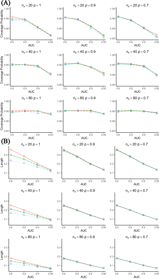
Figure 2: Estimated coverage probabilities and average lengths for 95% confidence intervals of the AUC for the log-normal distributions: (A) coverage probabilities, (B) average lengths. Three lines are shown: SRS-EL as solid lines with square markers ($\square$), BRSS-EL with $m=2$ as long-dashed lines with circle markers ($\circ$), and BRSS-EL with $m=4$ as dotted lines with triangle markers ($\triangle$).

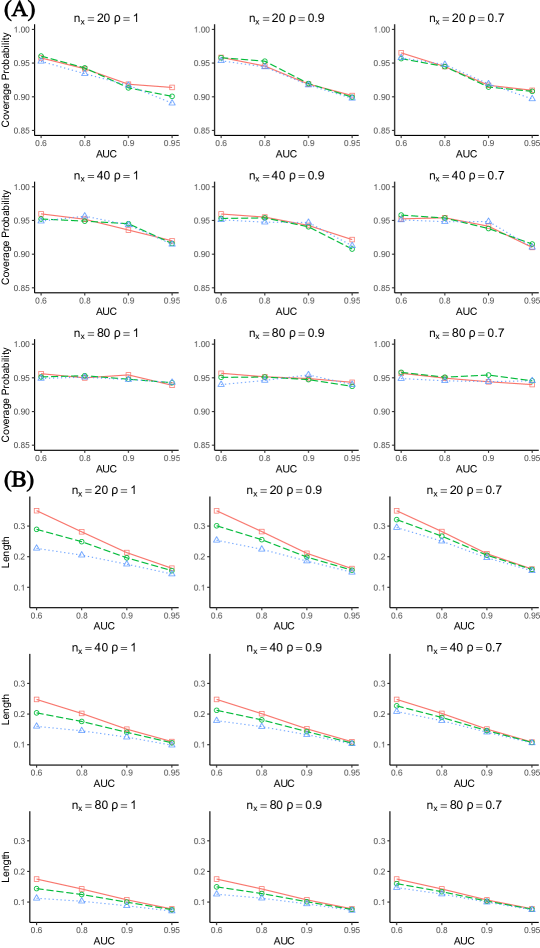
Figure 3: Estimated coverage probabilities and average lengths for 95% confidence intervals of the AUC for the uniform distributions: (A) coverage probabilities, (B) average lengths. Three lines are shown: SRS-EL as solid lines with square markers ($\square$), BRSS-EL with $m=2$ as long-dashed lines with circle markers ($\circ$), and BRSS-EL with $m=4$ as dotted lines with triangle markers ($\triangle$).

The simulation results indicate that the proposed BRSS-EL outperforms the other methods. Figures 1, 2, and 3 present the coverage probabilities and the average lengths for 95% confidence intervals of three methods: SRS-EL, BRSS-EL with $m=2$, and BRSS-EL with $m=4$. Except for small sample sizes and high AUC cases where efficient AUC estimation is difficult, the coverage probabilities of all three methods are close to the nominal level. BRSS-EL achieves shorter intervals in most cases while achieving similar coverage compared to SRS-EL.

The quality of judgment ranking affects the average length of RSS intervals. As $\rho$ gets smaller so that the quality of the judgment gets poorer, the BRSS-EL intervals get wider and become closer to SRS-EL. However, even with poor judgement ranking quality with $\rho=0.7$, the proposed method has a shorter interval than SRS-EL.

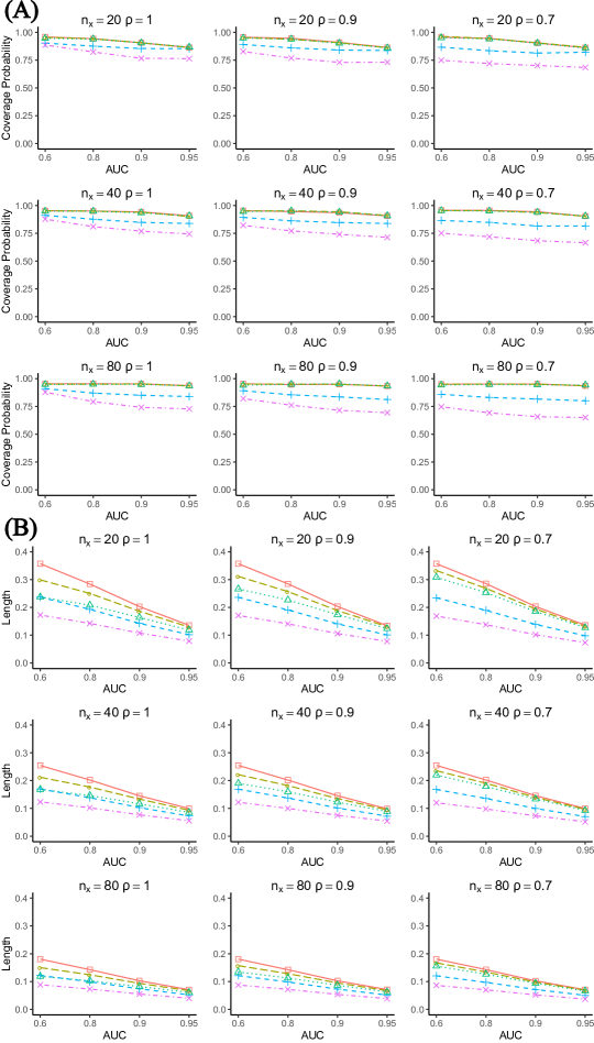
Figure 7: Estimated 95% confidence intervals of the AUC for normal distributions: (A) coverage probabilities, (B) average lengths. Five lines are shown: SRS-EL as solid lines with square markers ($\square$), BRSS-EL with $m=2$ as long-dashed lines with circle markers ($\circ$), BRSS-EL with $m=4$ as dotted lines with triangle markers ($\triangle$), BRSS-KER with $m=2$ as dashed lines with plus markers ($+$), and BRSS-KER with $m=4$ as dash-dot lines with cross markers ($\times$).

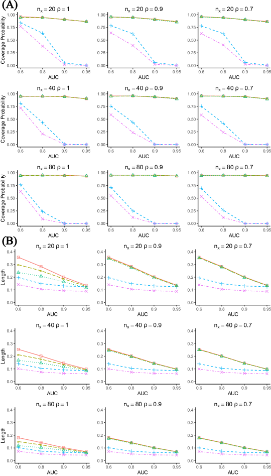
Figure 8: Estimated 95% confidence intervals of the AUC for log-normal distributions: (A) coverage probabilities, (B) average lengths. Five lines are shown: SRS-EL as solid lines with square markers ($\square$), BRSS-EL with $m=2$ as long-dashed lines with circle markers ($\circ$), BRSS-EL with $m=4$ as dotted lines with triangle markers ($\triangle$), BRSS-KER with $m=2$ as dashed lines with plus markers ($+$), and BRSS-KER with $m=4$ as dash-dot lines with cross markers ($\times$).

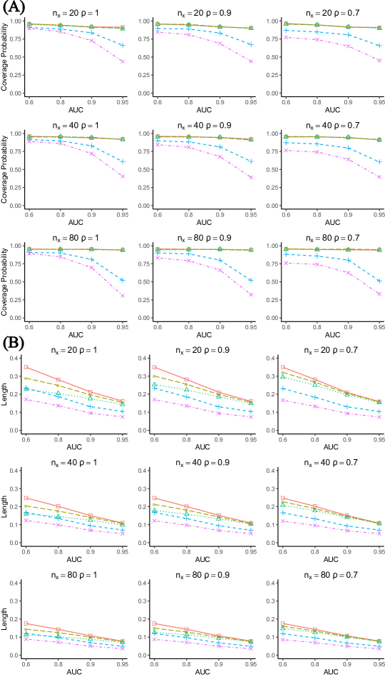
Figure 9: Estimated 95% confidence intervals of the AUC for uniform distributions: (A) coverage probabilities, (B) average lengths. Five lines are shown: SRS-EL as solid lines with square markers ($\square$), BRSS-EL with $m=2$ as long-dashed lines with circle markers ($\circ$), BRSS-EL with $m=4$ as dotted lines with triangle markers ($\triangle$), BRSS-KER with $m=2$ as dashed lines with plus markers ($+$), and BRSS-KER with $m=4$ as dash-dot lines with cross markers ($\times$).

The EL-based methods show higher coverage than BRSS-KER, particularly when the AUC is close to one. The results of BRSS-KER are reported in Figures 7, 8, and 9 in Appendix B because their coverage probabilities are low compared to the EL-based methods. Especially when the observations are sampled from the log-normal distributions with large AUC values, BRSS-KER performs poorly. The kernel estimates of the AUC are under-estimated, so BRSS-KER intervals usually do not include the true AUC value.

We also compare the computation time of BRSS-EL, SRS-EL, and BRSS-KER. We measure the time to run the simulations under three set sizes $m=n\in\{2,4,5\}$ with sample sizes $n_{x}=n_{y}=20$, $\rho=1$, $\delta=0.6$, and $X\sim N\left(0,1\right)$, and $Y\sim N\left(\sqrt{5}\Phi^{-1}(0.6),4\right)$. The SRS and BRSS samples are generated 5,000 times for each simulation setting and Intel Xeon E5-2695v4 2.1 GHz processors are used for computations. The total execution time for 5,000 replicates in each setting is reported in Table 1 in Appendix B. The EL-based methods (BRSS-EL and SRS-EL) take longer time than the kernel-based method (BRSS-KER) due to the computation of EL. The computation time of BRSS-EL is similar to that of SRS-EL, but it tends to decrease as the set size increases with fixed sample sizes.

3.2 Unbalanced RSS

We compare the EL-based methods using samples obtained by URSS (URSS-EL) and SRS (SRS-EL). For simplicity, only $Y$ is sampled by URSS whereas $X$ is obtained by BRSS with set sizes $m=n=2$. The number of the first and the second ranked sets of $Y$ is determined by the proportion $p_{y}$ such that $l_{1}=n_{y}p_{y}$ and $l_{2}=n_{y}(1-p_{y})$. When $p_{y}=0.5$, $Y$ is sampled by BRSS. We set $p_{y}\in\{0.3,0.4,0.5,0.6,0.7\}$ and assume perfect judgement ranking $\rho_{X}=\rho_{Y}=1$. The other simulation settings are the same as Section 3.1: URSS samples are generated 5,000 times for two sub-populations, $X$ and $Y$ are sampled from the three sets of distributions (normal, log-normal, and uniform), four AUC values are used $\delta\in\{0.6,0.8,0.9,0.95\}$, and sample sizes are $n_{x}=n_{y}\in\left\{20,40,80\right\}$. We also randomly generate SRS samples with the same AUC and sample size settings and compute SRS-EL results. The simulation results of BRSS-KER are not reported because it is proposed only for BRSS.

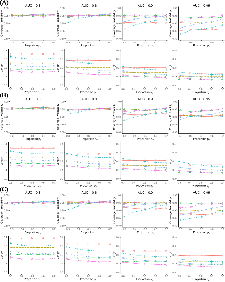
Figure 4: Coverage probabilities and average lengths for 95% confidence intervals of the AUC: (A) normal distribution, (B) log-normal distribution, (C) uniform distribution. Each plot presents six lines: SRS-EL of $n_{y}=20$ as solid lines with square markers ($\square$), URSS-EL of $n_{y}=20$ as dashed lines with cross markers ($+$), SRS-EL of $n_{y}=40$ as long-dashed lines with circle markers ($\circ$), URSS-EL of $n_{y}=40$ as dot-dashed lines with times markers ($\times$), SRS-EL of $n_{y}=80$ as dotted lines with triangle markers ($\triangle$), and URSS-EL of $n_{y}=80$ as two-dashed lines with diamond markers ($\diamond$).

URSS-EL performs better than BRSS-EL and SRS-EL under the well-designed URSS scheme. Figure 4 shows results of URSS-EL and SRS-EL simulations. When the AUC is close to one, taking a larger number of the first-ranked set samples of $Y$ (i.e., larger $p_{y}$ values) leads to coverage probabilities close to the nominal level and shorter intervals. In this case, the first-ranked set samples of $Y$ provide more information than the second-ranked set samples for the AUC estimation. Under the high AUC, the second-ranked set sample of $Y$ is most likely to be greater than the sample of $X$, so it is less informative. Therefore, obtaining a larger number of the first-ranked set samples of $Y$ enables better comparison of $F$ and $G$ for the high AUC. On the other hand, when the AUC is relatively low, the shortest interval of URSS-EL is achieved when samples are obtained by BRSS.

4 Case Studies

4.1 Application to Diabetes Data

We compare the AUC estimation methods using the US National Health and Nutrition Examination Survey (NHANES) collected from 2009 to 2010, available in the R package “NHANES” ⁴⁴. The NHANES dataset includes demographic, physical, and health information of 10,000 individuals. Although the NHANES data were obtained under complex survey design, we only consider two sub-populations: subjects who do not have diabetes ($X$) and have diabetes ($Y$). One of the best predictors for diabetes available in the NHANES dataset is the body mass index (BMI). The AUC value estimated using BMI is 0.73.

To generate SRS/BRSS samples, we treat the entire dataset of the 10,000 individuals as the “true” population, which is divided into two sub-populations, individuals with and without diabetes. In this simulation, we first set $n_{x}=n_{y}$ and let the sample sizes vary in the set $\{20,40,60,80\}$. For BRSS samples, we set $m=n$ and let the set sizes vary in the set $\{2,4\}$, and the numbers of cycles are determined by $k=n_{x}$/$m$ and $l=n_{y}$/$n$. In each simulation setting, we repeat the sampling procedure 5,000 times.

We use two concomitant variables, weight and total High-density lipoprotein cholesterol (TotChol), to illustrate how the results are affected by the quality of ranking. The weight has high Pearson correlations with BMI ($\rho_{X}=0.897$ and $\rho_{Y}=0.881$) thus it makes the high quality rankings. One the other hand, the TotChol has small negative Pearson correlations with BMI ($\rho_{X}=-0.294$ and $\rho_{Y}=-0.274$), which makes the poor quality rankings.

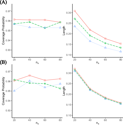
Figure 5: Coverage probabilities and average lengths for 95% confidence intervals of the AUC for the diabetes data: (A) weight is used as concomitant variable, (B) TotChol is used as concomitant variable. Three lines are shown: SRS-EL as solid lines with square markers ($\square$), BRSS-EL with $m=2$ as long-dashed lines with circle markers ($\circ$), and BRSS-EL with $m=4$ as dotted lines with triangle markers ($\triangle$).

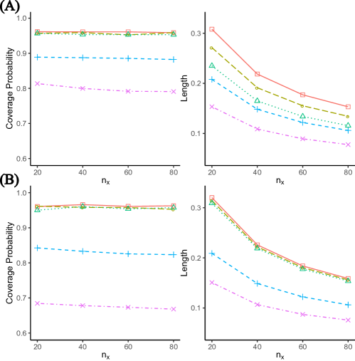
Figure 10: Coverage probabilities and average lengths for 95% confidence intervals of the AUC for the diabetes data: (A) weight is used as concomitant variable, (B) TotChol is used as concomitant variable. Five lines are shown: SRS-EL as solid lines with square markers ($\square$), BRSS-EL with $m=2$ as long-dashed lines with circle markers ($\circ$), BRSS-EL with $m=4$ as dotted lines with triangle markers ($\triangle$), BRSS-KER with $m=2$ as dashed lines with plus markers ($+$), and BRSS-KER with $m=4$ as dash-dot lines with cross markers ($\times$).

Figure 5 shows coverage probabilities and average lengths for 95% confidence intervals of SRS-EL, BRSS-EL with $m=2$, and BRSS-EL with $m=4$. When the weight is used for judgement ranking, BRSS-EL has shorter intervals than SRS-EL while maintaining similar coverage probabilities. On the other hand, when the TotChol is used as the concomitant variable, the BRSS-EL intervals are still slightly shorter than the SRS-EL intervals despite the lower ranking quality. In both cases, coverage probabilities of BRSS-EL are closer to 0.95 than that of SRS-EL. The complete results that include BRSS-KER are given in Figure 10 in Appendix B. BRSS-KER has the shortest intervals, but its coverage probabilities are the lowest.

The result suggests that BRSS-EL yields better inferences over SRS-EL regardless of the quality of the rankings. If the concomitant variable is informative, such as the weight in this application, the proposed method gives more efficient inference than the other methods. Even in the worst case when the concomitant variable is not informative, such as the TotChol, BRSS-EL achieves results similar to SRS-EL. As a result, our method gives better or at least as good results as SRS-EL.

4.2 Application to Chronic Kidney Disease Data

Chronic kidney disease (CKD) refers to a condition that the kidneys are gradually damaged and cannot filter blood as needed. Diabetes is a major cause of CKD. In 2008, about 44% of new kidney failure was due to diabetes ⁴⁵. An early diagnosis of CKD is important because early treatment may prevent the kidney from being further damaged. Therefore, it is suggested that a person with diabetes monitors the signs of CKD.

There are two common markers that evaluate kidney functions: 1) a blood test that estimates glomerular filtration rate (GFR), and 2) a urine test that measures albumin to creatinine ratio (ACR). GFR estimates how much blood is flowing each minute and it indicates how well a kidney is working. GFR is estimated using multiple factors such as serum creatinine level, age, gender, and ethnicity. ACR is used to estimate the excretion of urinary albumin. The damaged kidney does not filter proteins well, and it leads to a high level of urinary albumin, one of the proteins that can be found in urine. If people have GFR less than 60 $ml/min/1.73m^{2}$ or ACR greater than 30 $mg/g$ for three months, then they are at risk of decreased kidney function ⁴⁶.

We use 3,051 subjects with diabetes ages 21 to 79 in the NHANES datasets from 2009 to 2018. We consider two sub-populations that do not have CKD ($X$) and has CKD ($Y$). The subjects are classified to have CKD if their GFR$<$60 or ACR$>$30. We want to note that three months of GFR and ACR information is needed to diagnose CKD. However, we only use one-time GFR and ACR records for simplicity. We estimate GFR using the chronic kidney disease epidemiology collaboration equation ⁴⁷, which is recommended for reporting GFR in adults ⁴⁸.

We estimate the AUC for CKD among subjects with diabetes using GFR. The estimated AUC calculated by the negative GFR is $0.757$. The negative GFR is used here because low GFR indicates poor kidney function. One of the key factors in estimating GFR is the serum creatinine level, which should be obtained through a blood test. In some cases, blood tests and serum creatinine measurements may not be readily available. On the other hand, age is another important variable in GFR estimation and is easier to obtain. It is known that GFR tends to decrease with age ⁴⁹. In this study, age is used as the concomitant variable for GFR. In our dataset, the correlations between age and the negative GFR for non-CKD and CKD populations are $\rho_{X}=0.633$ and $\rho_{Y}=0.510$, respectively.

We sample under the same setting of Section 4.1: randomly generate samples 5,000 times from two sub-populations with sample sizes $n_{x}=n_{y}\in\left\{20,40,60,80\right\}$, $m=n\in\left\{2,4\right\}$, and $k=n_{x}$/$m$ and $l=n_{y}$/$n$. Figure 6 presents coverage probabilities and average lengths for 95% confidence intervals of the AUC for SRS-EL, BRSS-EL with $m=2$, and BRSS-EL with $m=4$.

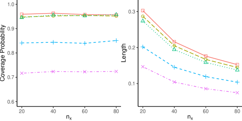
Figure 11: Coverage probabilities and average lengths for 95% confidence intervals of the AUC for the CKD data when age is used as the concomitant variable. Five lines are shown: SRS-EL as solid lines with square markers ($\square$), BRSS-EL with $m=2$ as long-dashed lines with circle markers ($\circ$), BRSS-EL with $m=4$ as dotted lines with triangle markers ($\triangle$), BRSS-KER with $m=2$ as dashed lines with plus markers ($+$), and BRSS-KER with $m=4$ as dash-dot lines with cross markers ($\times$).

Using age as the concomitant variable in BRSS-EL leads to more efficient inference on the AUC than the other methods. BRSS-EL and SRS-EL achieve similar coverage probabilities close to $0.95$, while BRSS-EL has coverage probabilities closer to the nominal level. Also, the average lengths of the confidence intervals of BRSS-EL are shorter than SRS-EL regardless of the sample size. The BRSS-KER results are presented in Figure 11 in Appendix B. Although BRSS-KER has the shortest average lengths of the confidence intervals, its coverage probabilities are lower than the others.

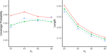
Figure 6: Coverage probabilities and average lengths for 95% confidence intervals of the AUC for the CKD data when age is used as the concomitant variable. Three lines are shown: SRS-EL as solid lines with square markers ($\square$), BRSS-EL with $m=2$ as long-dashed lines with circle markers ($\circ$), and BRSS-EL with $m=4$ as dotted lines with triangle markers ($\triangle$).

5 Discussion

We propose the EL method that finds the confidence interval of the AUC using data obtained from balanced and unbalanced RSS. We show that the EL-based confidence intervals can be found by the scaled chi-square distributions. The proposed method performs the best in the sense that its confidence interval achieves the coverage probability close to the nominal level with the shorter length. Simulation studies show that the proposed method performs well regardless of distributions of diseased and non-diseased subjects and AUC values. We apply the proposed approach to diabetes and CKD data and show it outperforms the other methods.

Our study suggests that the well-designed RSS may lead to more efficient inference on the AUC. First, the proposed method shows improvement over SRS-EL regardless of the quality of ranking. Therefore, implementing RSS and estimating the confidence interval of the AUC using EL is a better strategy than SRS-EL. Second, one can obtain improved results by carefully assigning the number of ranked sets in URSS. For example, simulation studies show that when the AUC value is close to one, taking a larger number of low-rank samples from the diseased population in URSS leads to improved inference. This could be useful in practice when some prior information of the AUC is available.

The proposed AUC estimator treats the X and Y samples in an asymmetric way; it uses the distribution function of non-diseased subjects $F$ as a reference and constructs the confidence interval for $P(X\leq Y)$. However, the AUC can also be estimated using the distribution of diseased subjects $G$ as the reference and then estimating the confidence interval for $1-P(Y<X)$. Let the placement value of $X$ be $W_{ij}=G(X_{[i]j})$, a proportion of diseased subjects whose measurements are smaller than $X_{[i]j}$. The AUC can be obtained by $E\left[\sum\limits_{i=1}^{m}\sum\limits_{j=1}^{k}\frac{1}{mk}\left(1-W_{ij}\right)\right]=E[1-G(X)]=\delta$. The profile EL for the AUC of BRSS can be constructed as

$$L_{BRSS}^{*}(\delta_{0})=\sup\left\{\prod\limits_{i=1}^{m}\prod\limits_{j=1}^{k}q_{ij}:\sum\limits_{i=1}^{m}\sum\limits_{j=1}^{k}q_{ij}=1,\sum\limits_{i=1}^{m}\sum\limits_{j=1}^{k}q_{ij}\left(1-W_{ij}-\delta_{0}\right)=0\right\},$$

where $\sum_{i=1}^{m}\sum_{j=1}^{k}q_{ij}=1$ and $q_{ij}\geq 0$ for all $i=1,\ldots,m$ and $j=1,\ldots,k$. Similar to Section 2, $W_{ij}$ can be estimated by the empirical distribution $\widehat{W}_{ij}=\widehat{G}\left(X_{[i]j}\right)=\frac{1}{nl}\sum\limits_{r=1}^{n}\sum\limits_{s=1}^{l}\phi\left(Y_{[r]s},X_{[i]j}\right)$ and the empirical log-likelihood ratio becomes

$$l_{BRSS}^{*}(\delta_{0})=2\sum\limits_{i=1}^{m}\sum\limits_{j=1}^{k}\log\left(1+\lambda\left(1-\widehat{W}_{ij}-\delta_{0}\right)\right).$$

The asymptotic distribution of $l_{BRSS}^{*}(\delta_{0})$ also follows the scaled chi-square distribution

$$r^{*}_{BRSS}(\delta_{0})l_{BRSS}^{*}(\delta_{0})\rightarrow\chi^{2}_{1},\text{ where}$$

$$r^{*}_{BRSS}(\delta_{0})=\frac{nl}{mk+nl}\frac{\sum\limits_{i=1}^{m}\sum\limits_{j=1}^{k}\frac{1}{mk}\left(1-\widehat{W}_{ij}-\delta_{0}\right)^{2}}{S_{BRSS}^{2}}.$$

A similar extension can also be applied to URSS. In practice, it would be natural to set $F$ as the reference because the number of the non-diseased sample $n_{x}$ is expected to be larger than the number of the diseased sample $n_{y}$. Table 2 compares the coverage probabilities and average lengths of the AUC for two approaches when $X$ and $Y$ are sampled using BRSS from the normal distributions presented in Section 3.1 with $n_{x}\in\{40,100,200\}$, $n_{y}=40$, $m=n=2$, $\rho=1$, and $\delta=0.8$. As $n_{x}$ gets larger, the confidence interval of using $F$ as the reference becomes narrower while maintaining the coverage probability close to the nominal level. On the other hand, the length of the confidence interval using $G$ as the reference has little change, but its standard deviation gets larger as $n_{x}$ increases.

An interesting future work is using the nonparametric maximum likelihood estimator (NPMLE) $F^{*}$ of Kvam and Samaniego⁵⁰ instead of the empirical distribution $\widehat{F}$ of Stokes and Sager¹¹. The NPMLE assigns different probabilities to observations and is known to perform better than the empirical distribution. Thus, implementing the NPMLE could further improve the efficiency of inference on the AUC. Another interesting topic is to determine the optimal number of set sizes for the AUC estimation. A few studies have investigated the optimal set size for one-population problems by considering the quality of judgment ranking, the impact of imperfect rankings, and cost of sampling^{51, 52}. However, for two-population problems such as the AUC estimation, the cost of recruiting units from one sub-population might be much more than that from the other. Thus, it might be worth a formal investigation in the future.

Conflict of interest

The authors declare no potential conflict of interests.

Data Availability Statement

All data used in simulation studies are generated randomly and the NHANES data used in the case studies are imported from https://www.cdc.gov/nchs/nhanes/. The R code used to generate, import, and analyze the data used in this paper is publicly available at the URL:https://github.com/chulmoon/EL-RSS-AUC.

Appendix A Proof of Theorems

Lemma A.1.

Under the assumptions of Theorem 2.1,

(i) $$\sum\limits_{r=1}^{n}\sum\limits_{s=1}^{l}\frac{1}{nl}\left(1-\widehat{U}_{rs}-\delta_{0}\right)^{2}\xrightarrow{p}\frac{1}{n}\left(\sum\limits_{r=1}^{n}\left(\sigma_{0[r]}^{Y}\right)^{2}+\sum\limits_{r=1}^{n}\left(\delta_{0[r]}^{Y}-\delta_{0}\right)^{2}\right),$$

$$\text{where }\sigma_{[r]}^{Y}=E\left[\left(F(Y_{[r]})-\delta_{0[r]}^{Y}\right)^{2}\right],$$

$$\text{and }\delta_{0[r]}^{Y}\text{ is the true AUC when the $r$th order statistic from a SRS of size $n$ of diseased subjects is used}.$$

(ii) $$\left(\frac{mknl}{mk+nl}\right)^{1/2}\frac{\sum\limits_{r=1}^{n}\sum\limits_{s=1}^{l}\frac{1}{nl}\left(1-\widehat{U}_{rs}-\delta_{0}\right)}{S_{BRSS}}\xrightarrow{D}N(0,1).$$

Proof A.2.

(i) Using the uniform consistency of the empirical distribution $\widehat{F}$ we have,

$$\sum\limits_{r=1}^{n}\sum\limits_{s=1}^{l}\frac{1}{nl}\left(1-\widehat{U}_{rs}-\delta_{0}\right)^{2} = \sum\limits_{r=1}^{n}\sum\limits_{s=1}^{l}\frac{1}{nl}\left(\widehat{F}(Y_{[r]s})-\delta_{0}\right)^{2}$$

$$= \sum\limits_{r=1}^{n}\sum\limits_{s=1}^{l}\frac{1}{nl}\left(\widehat{F}(Y_{[r]s})-\delta_{0[r]}^{Y}+\delta_{0[r]}^{Y}-\delta_{0}\right)^{2}$$

$$= \sum\limits_{r=1}^{n}\sum\limits_{s=1}^{l}\frac{1}{nl}\left(\widehat{F}(Y_{[r]s})-\delta_{0[r]}^{Y}\right)^{2}+\sum\limits_{r=1}^{n}\sum\limits_{s=1}^{l}\frac{1}{nl}\left(\delta_{0[r]}^{Y}-\delta_{0}\right)^{2}$$

$$\xrightarrow{p} \frac{1}{n}\left(\sum\limits_{r=1}^{n}\left(\sigma_{[r]}^{Y}\right)^{2}+\sum\limits_{r=1}^{n}\left(\delta_{0[r]}^{Y}-\delta_{0}\right)^{2}\right).$$

(ii) For RSS, the distribution functions of diseased and non-diseased subjects can be written as $G(x)=\frac{1}{n}\sum\limits_{r=1}^{n}G_{[r]}(x)$ and $F(x)=\frac{1}{m}\sum\limits_{i=1}^{m}F_{[i]}(x)$, respectively, regardless of the quality of the judgement ranking ⁵³. By simple calculations,

$$\text{Var}(\widehat{\delta}_{BRSS}) = \frac{1}{mknl}\left\{nl\left(\beta-\frac{1}{m}\sum\limits_{i=1}^{m}\left(\delta_{[i]}^{X}\right)^{2}\right)+mk\left(\alpha-\frac{1}{n}\sum\limits_{r=1}^{n}\left(\delta_{[r]}^{Y}\right)^{2}\right)\right.$$

$$\left.+\left(\delta_{0}-\overline{\delta}_{0}^{2}-\left(\overline{\beta}-\overline{\delta}_{0}^{2}\right)-\left(\overline{\alpha}-\overline{\delta}_{0}^{2}\right)\right)\right\},$$

where $\beta=\int_{0}^{1}\left(1-G(x)\right)^{2}dF(x)$, $\overline{\beta}=\int_{0}^{1}\frac{1}{n}\sum\limits_{r=1}^{n}\left(1-G_{[r]}(x)\right)^{2}dF(x)$, $\alpha=\int_{0}^{1}F^{2}(x)dG(x)$, $\overline{\alpha}=\int_{0}^{1}\frac{1}{m}\sum\limits_{i=1}^{m}F_{[i]}^{2}(x)dG(x)$, $\delta_{[r]}^{Y}=P(X\leq Y_{[r]})$, $\delta_{[i]}^{X}=P(X_{[i]}\leq Y)$, and $\overline{\delta}_{0}^{2}=\frac{1}{mn}\sum\limits_{i=1}^{m}\sum\limits_{r=1}^{n}\left(P(X_{[i]}<Y_{[r]})\right)^{2}$.

Then,

$$nlE\left[\left(S_{BRSS}^{10}\right)^{2}\right] = \sum\limits_{i=1}^{m}\sum\limits_{j=1}^{k}\frac{nl}{m(k-1)}E\left[V_{BRSS}^{10}(X_{[i]j})V_{BRSS}^{10}(X_{[i]j})\right]-\sum\limits_{i=1}^{m}\frac{knl}{m(k-1)}E\left[\overline{V}_{BRSS[i]}^{10}\overline{V}_{BRSS[i]}^{10}\right]$$

$$= nl\left(\beta-\frac{1}{m}\sum\limits_{i=1}^{m}\left(\delta_{[i]}^{X}\right)^{2}\right)-\overline{\beta}-\overline{\alpha}+\delta_{0}-\overline{\delta}_{0}^{2},$$

$$mkE\left[\left(S_{BRSS}^{01}\right)^{2}\right] = \sum\limits_{r=1}^{n}\sum\limits_{s=1}^{l}\frac{mk}{n(l-1)}E\left[V_{BRSS}^{01}(Y_{[r]s})V_{BRSS}^{01}(Y_{[r]s})\right]-\sum\limits_{r=1}^{n}\frac{mkl}{n(l-1)}E\left[\overline{V}_{BRSS[r]}^{01}\overline{V}_{BRSS[r]}^{01}\right]$$

$$= mk\left(\alpha-\frac{1}{n}\sum\limits_{r=1}^{n}\left(\delta_{[r]}^{Y}\right)^{2}\right)-\overline{\alpha}-\overline{\beta}+\delta_{0}-\overline{\delta}_{0}^{2}.$$

Therefore,

$$E\left[S_{BRSS}^{2}\right] = E\left[\frac{nl\left(S_{BRSS}^{10}\right)^{2}+mk\left(S_{BRSS}^{01}\right)^{2}}{mk+nl}\right]$$

$$= \text{Var}\left(\left(\frac{mknl}{mk+nl}\right)^{\frac{1}{2}}(\widehat{\delta}_{BRSS}-\delta_{0})\right)+\frac{\delta_{0}-\overline{\delta}_{0}^{2}-\left(\overline{\beta}-\overline{\delta}_{0}^{2}\right)-\left(\overline{\alpha}-\overline{\delta}_{0}^{2}\right)}{mk+nl}.$$

Now, we will show that the bias of $S_{BRSS}^{2}$ is less than $\frac{\delta_{0}-\overline{\delta}_{0}^{2}}{mk+nl}$. Let the counter function be

$$\overline{\phi}(X_{[i]j},Y_{[r]s})=\phi(X_{[i]j},Y_{[r]s})-\overline{\delta}_{ir}-\left(\phi_{10}(X_{[i]j})-\overline{\delta}_{ir}\right)-\left(\phi_{01}(Y_{[r]s})-\overline{\delta}_{ir}\right),$$

where $\phi_{10}(x_{[i]j})=\sum\limits_{r=1}^{n}\sum\limits_{s=1}^{l}\frac{1}{nl}E\left[\phi(x_{[i]j},Y_{[r]s})\right]$, $\phi_{01}(y_{[r]s})=\sum\limits_{i=1}^{m}\sum\limits_{j=1}^{k}\frac{1}{mk}E\left[\phi(X_{[i]j},y_{[r]s})\right]$ and $\overline{\delta}_{ir}=P(X_{[i]}<Y_{[r]})$.

Then,

$$\frac{1}{mknl}\sum\limits_{i=1}^{m}\sum\limits_{j=1}^{k}\sum\limits_{r=1}^{n}\sum\limits_{s=1}^{l}E\left[\overline{\phi}^{2}(X_{[i]j},Y_{[r]s})\right]$$

$$= \frac{1}{mknl}\sum\limits_{i=1}^{m}\sum\limits_{j=1}^{k}\sum\limits_{r=1}^{n}\sum\limits_{s=1}^{l}E\left[\left(\phi(X_{[i]j},Y_{[r]s})-\overline{\delta}_{ir}-\left(\phi_{10}(X_{[i]j})-\overline{\delta}_{ir}\right)-\left(\phi_{01}(Y_{[r]s})-\overline{\delta}_{ir}\right)\right)^{2}\right]$$

$$= \delta_{0}-\overline{\delta}_{0}^{2}-\left(\overline{\alpha}-\overline{\delta}_{0}^{2}\right)-\left(\overline{\beta}-\overline{\delta}_{0}^{2}\right)\geq 0.$$

Because

$$\frac{1}{mknl}\sum\limits_{i=1}^{m}\sum\limits_{j=1}^{k}\sum\limits_{r=1}^{n}\sum\limits_{s=1}^{l}E\left[\left(\phi_{10}(X_{[i]j})-\overline{\delta}_{ir}\right)^{2}\right]=\overline{\alpha}-\overline{\delta}_{0}^{2}\geq 0,$$

$$\frac{1}{mknl}\sum\limits_{i=1}^{m}\sum\limits_{j=1}^{k}\sum\limits_{r=1}^{n}\sum\limits_{s=1}^{l}E\left[\left(\phi_{01}(Y_{[r]s})-\overline{\delta}_{ir}\right)^{2}\right]=\overline{\beta}-\overline{\delta}_{0}^{2}\geq 0,$$

it implies

$$0\leq\left(\overline{\alpha}-\overline{\delta}_{0}^{2}\right)+\left(\overline{\beta}-\overline{\delta}_{0}^{2}\right)\leq\delta_{0}-\overline{\delta}_{0}^{2}.$$ (9)

By (9), we get the upper bound of the bias of $S^{2}$.

Let

$$T(X_{[1]1},\ldots,X_{[m]k},Y_{[1]1},\ldots,Y_{[n]l})$$

$$=\frac{1}{mk}\sum\limits_{i=1}^{m}\sum\limits_{j=1}^{k}\left(\phi_{10}(X_{[i]j})-\delta_{[i]}^{X}\right)+\frac{1}{nl}\sum\limits_{r=1}^{n}\sum\limits_{s=1}^{l}\left(\phi_{01}(Y_{[r]s})-\delta_{[r]}^{Y}\right).$$

Then,

$$\frac{mknl}{mk+nl}E\left[\left\{T(X_{[1]1},\ldots,X_{[m]k},Y_{[1]1},\ldots,Y_{[n]l})-(\widehat{\delta}_{BRSS}-\delta_{0})\right\}^{2}\right]$$

$$= \frac{\delta_{0}-\overline{\delta}_{0}^{2}-\left(\overline{\alpha}-\overline{\delta}_{0}^{2}\right)-\left(\overline{\beta}-\overline{\delta}_{0}^{2}\right)}{mk+nl}$$

$$\leq \frac{\delta_{0}-\overline{\delta}_{0}^{2}}{mk+nl}$$

$$= O(\max(k,l)^{-1}).$$

By Chebyshev’s inequality,

$$\frac{mknl}{mk+nl}\left(\widehat{\delta}_{BRSS}-\delta_{0}\right)\xrightarrow{p}\frac{mknl}{mk+nl}T\left(X_{[1]1},\ldots,X_{[m]k},Y_{[1]1},\ldots,Y_{[n]l}\right).$$ (10)

As $k\rightarrow\infty$ and $l\rightarrow\infty$, by the central limit theorem,

$$\frac{1}{\sqrt{mk}}\sum\limits_{i=1}^{m}\sum\limits_{j=1}^{k}\phi_{10}(X_{[i]j}) \xrightarrow{D} N\left(0,\overline{\beta}-\overline{\delta}_{0}^{2}\right)$$ (11)

$$\frac{1}{\sqrt{nl}}\sum\limits_{r=1}^{n}\sum\limits_{s=1}^{l}\phi_{01}(Y_{[r]s}) \xrightarrow{D} N\left(0,\overline{\alpha}-\overline{\delta}_{0}^{2}\right).$$ (12)

Thus from (10), (11), (12), and $S_{BRSS}^{2}\xrightarrow{p}\text{Var}\left(\frac{mknl}{mk+nl}\left(\widehat{\delta}_{BRSS}-\delta_{0}\right)\right)$, Lemma A.1(ii) is proved.

Proof A.3 (Proof of Theorem 2.1).

Using Lemma A.1 and the similar arguments of Owen⁷, we can show that $|\lambda|=O_{p}(n_{y}^{-1/2})$ and

$$\lambda=\frac{\sum\limits_{r=1}^{n}\sum\limits_{s=1}^{l}\left(1-\widehat{U}_{rs}-\delta_{0}\right)}{\sum\limits_{r=1}^{n}\sum\limits_{s=1}^{l}\left(1-\widehat{U}_{rs}-\delta_{0}\right)^{2}}+O_{p}(n_{y}^{-1/2}).$$ (13)

By applying Taylor expansion to equation (4) in Section 2.2,

$$l(\delta_{0})=2\sum\limits_{r=1}^{n}\sum\limits_{s=1}^{l}\left(\lambda\left(1-\widehat{U}_{rs}-\delta_{0}\right)-\frac{1}{2}\left(\lambda\left(1-\widehat{U}_{rs}-\delta_{0}\right)\right)^{2}\right)+R_{n_{y}},$$

where $R_{n_{y}}\leq C\sum\limits_{r=1}^{n}\sum\limits_{s=1}^{l}\left|\lambda\left(1-\widehat{U}_{rs}-\delta_{0}\right)\right|^{3}$ for some constant $C$. Because $F\in[0,1]$ and so the third moment of $F(Y_{[r]s})$ is finite, and $|\lambda|=O_{p}(n_{y}^{-1/2})$,

$$\left|R_{n_{y}}\right|\leq C\sum\limits_{r=1}^{n}\sum\limits_{s=1}^{l}\left|\lambda\left(1-\widehat{U}_{rs}-\delta_{0}\right)\right|^{3}=C\sum\limits_{r=1}^{n}\sum\limits_{s=1}^{l}\left|\lambda\left(\widehat{F}(Y_{[r]s})-\delta_{0}\right)\right|^{3}\leq C\left|\lambda\right|^{3}n_{y}=O_{p}(n_{y}^{-1/2}).$$

Also, equation (3) in Section 2.2 can be expressed as,

$$0 = \sum\limits_{r=1}^{n}\sum\limits_{s=1}^{l}\frac{\left(1-\widehat{U}_{rs}-\delta_{0}\right)}{1+\lambda\left(1-\widehat{U}_{rs}-\delta_{0}\right)}$$ (14)

$$= \sum\limits_{r=1}^{n}\sum\limits_{s=1}^{l}\lambda\left(1-\widehat{U}_{rs}-\delta_{0}\right)\left(1-\lambda\left(1-\widehat{U}_{rs}-\delta_{0}\right)+\frac{\left(\lambda\left(1-\widehat{U}_{rs}-\delta_{0}\right)\right)^{2}}{1+\lambda\left(1-\widehat{U}_{rs}-\delta_{0}\right)}\right)$$

$$= \sum\limits_{r=1}^{n}\sum\limits_{s=1}^{l}\lambda\left(1-\widehat{U}_{rs}-\delta_{0}\right)-\sum\limits_{r=1}^{n}\sum\limits_{s=1}^{l}\left(\lambda\left(1-\widehat{U}_{rs}-\delta_{0}\right)\right)^{2}+\sum\limits_{r=1}^{n}\sum\limits_{s=1}^{l}\frac{\left(\lambda\left(1-\widehat{U}_{rs}-\delta_{0}\right)\right)^{3}}{1+\lambda\left(1-\widehat{U}_{rs}-\delta_{0}\right)}$$

$$= \sum\limits_{r=1}^{n}\sum\limits_{s=1}^{l}\lambda\left(1-\widehat{U}_{rs}-\delta_{0}\right)-\sum\limits_{r=1}^{n}\sum\limits_{s=1}^{l}\left(\lambda\left(1-\widehat{U}_{rs}-\delta_{0}\right)\right)^{2}+O_{p}(n_{y}^{-1/2}),$$

Therefore,

$$r(\delta_{0})l(\delta_{0}) = 2r(\delta_{0})\sum\limits_{r=1}^{n}\sum\limits_{s=1}^{l}\left(\lambda\left(1-\widehat{U}_{rs}-\delta_{0}\right)-\frac{1}{2}(\lambda\left(1-\widehat{U}_{rs}-\delta_{0}\right))^{2}\right)+R_{n_{y}}$$

$$= r(\delta_{0})\left(2\sum\limits_{r=1}^{n}\sum\limits_{s=1}^{l}\lambda\left(1-\widehat{U}_{rs}-\delta_{0}\right)-\sum\limits_{r=1}^{n}\sum\limits_{s=1}^{l}\left(\lambda\left(1-\widehat{U}_{rs}-\delta_{0}\right)\right)^{2}\right)+O_{p}(n_{y}^{-1/2})$$

$$= r(\delta_{0})\left(\sum\limits_{r=1}^{n}\sum\limits_{s=1}^{l}\left(\lambda\left(1-\widehat{U}_{rs}-\delta_{0}\right)\right)^{2}\right)+O_{p}(n_{y}^{-1/2})\text{, using (\ref{eq:10})}$$

$$= r(\delta_{0})\frac{\left(\sum\limits_{r=1}^{n}\sum\limits_{s=1}^{l}\left(1-\widehat{U}_{rs}-\delta_{0}\right)\right)^{2}}{\sum\limits_{r=1}^{n}\sum\limits_{s=1}^{l}\left((1-\widehat{U}_{rs}-\delta_{0}\right)^{2}}+O_{p}(n_{y}^{-1/2})\text{, by plugging (\ref{eq:9})}$$

$$= \frac{mknl}{mk+nl}\frac{\left(\sum\limits_{r=1}^{n}\sum\limits_{s=1}^{l}\frac{1}{nl}\left(1-\widehat{U}_{rs}-\delta_{0}\right)\right)^{2}}{S^{2}}+O_{p}(n_{y}^{-1/2})$$

$$= \left[\left(\frac{mknl}{mk+nl}\right)^{1/2}\frac{\sum\limits_{r=1}^{n}\sum\limits_{s=1}^{l}\frac{1}{nl}\left(1-\widehat{U}_{rs}-\delta_{0}\right)}{S}\right]^{2}+O_{p}(n_{y}^{-1/2})$$

$$\xrightarrow{D} \chi^{2}_{1}.$$

Lemma A.4.

Under the assumptions of Theorem 2.2,

(i) $$\sum\limits_{r=1}^{n}\sum\limits_{s=1}^{l_{r}}\frac{1}{nl_{r}}\left(1-\widehat{U}_{rs}-\delta_{0}\right)^{2}\xrightarrow{p}\frac{1}{n}\left(\sum\limits_{r=1}^{n}\left(\sigma_{0[r]}^{Y}\right)^{2}+\sum\limits_{r=1}^{n}\left(\delta_{0[r]}^{Y}-\delta_{0}\right)^{2}\right),$$

$$\text{where }\sigma_{[r]}^{Y}=E\left[\left(F(Y_{[r]})-\delta_{0[r]}^{Y}\right)^{2}\right],$$

$$\text{and }\delta_{0[r]}^{Y}\text{ is the true AUC when the $r$th order statistic from a SRS of size $n$ of diseased subjects is used}.$$

(ii) $$\left(\frac{n_{x}n_{y}}{n_{x}+n_{y}}\right)^{1/2}\frac{\sum\limits_{r=1}^{n}\sum\limits_{s=1}^{l_{r}}\frac{1}{nl_{r}}\left(1-\widehat{U}_{rs}-\delta_{0}\right)}{S}\xrightarrow{D}N(0,1).$$

Proof A.5.

The proof is a simple modification of Lemma A.1. By replacing $l$ with $l_{r}$, $k$ with $k_{i}$, $nl$ with $n_{y}$, $mk$ with $n_{x}$ and following the similar steps, Lemma A.4 can be proved.

Proof A.6 (Proof of Theorem 2.2).

Using Lemma A.4 and similar steps used in Theorem 2.1, Theorem 2.2 can be proved.

Appendix B Tables and Figures

Table 1: Comparison of the computation time. The total execution time for 5,000 replicates in each setting is reported.

	Time (seconds)
Methods	$m=n=2$	$m=n=4$	$m=n=5$
SRS-EL	531	532	532
BRSS-EL	577	480	453
BRSS-KER	135	140	144

Table 2: Coverage probabilities and average lengths for 95% confidence intervals of the AUC for two approaches: 1) using $F$ as the reference ($P(X\leq Y)$) and 2) using $G$ as the reference ($1-P(Y<X)$). The BRSS samples are generated 1,000 times for $X$ and $Y$, respectively.

Sample size	Reference distribution	Length (standard deviation)	Coverage probability
$n_{x}=40$, $n_{y}=40$	Non-diseased, $F$	0.176 (0.018)	0.942
	Diseased, $G$	0.187 (0.027)	0.948
$n_{x}=100$, $n_{y}=40$	Non-diseased, $F$	0.168 (0.017)	0.950
	Diseased, $G$	0.187 (0.032)	0.966
$n_{x}=200$, $n_{y}=40$	Non-diseased, $F$	0.164 (0.018)	0.945
	Diseased, $G$	0.186 (0.034)	0.963

References

• 1 Bamber D. The area above the ordinal dominance graph and the area below the receiver operating characteristic graph. J Math Psychol 1975; 12(4): 387-415.
• 2 Hanley JA, McNeil BJ. The meaning and use of the area under a receiver operating characteristic (ROC) curve. Radiol 1982; 143(1): 29-36.
• 3 Qin G, Zhou XH. Empirical likelihood inference for the area under the ROC curve. Biometrics 2006; 62(2): 613-622.
• 4 Zou KH, Hall WJ, Shapiro DE. Smooth non-parametric receiver operating characteristic (ROC) curves for continuous diagnostic tests. Stat Med 1997; 16(19): 2143-2156.
• 5 Lloyd CJ. Using smoothed receiver operating characteristic curves to summarize and compare diagnostic systems. J Am Stat Assoc 1998; 93(444): 1356-1364.
• 6 Owen AB. Empirical likelihood ratio confidence intervals for a single functional. Biometrika 1988; 75(2): 237-249.
• 7 Owen AB. Empirical likelihood ratio confidence regions. Ann Stat 1990; 18(1): 90-120.
• 8 Owen AB. Empirical likelihood for linear models. Ann Stat 1991; 19(4): 1725-1747.
• 9 DiCiccio TJ, Hall P, Romano JP. Empirical likelihood is Bartlett-correctable. Ann Stat 1991; 19(2): 1053-1061.
• 10 McIntyre GA. A method for unbiased selective sampling using ranked sets. Aust J Agric Res 1952; 3(4): 385-390.
• 11 Stokes SL, Sager TW. Characterization of a ranked-set sample with application to estimating distribution functions. J Am Stat Assoc 1988; 83(402): 374-381.
• 12 Bohn LL, Wolfe DA. Nonparametric two-sample procedures for ranked-set samples data. J Am Stat Assoc 1992; 87(418): 552-561.
• 13 Bohn LL, Wolfe DA. The effect of imperfect judgment rankings on properties of procedures based on the ranked-set samples analog of the Mann-Whitney-Wilcoxon statistic. J Am Stat Assoc 1994; 89(425): 168-176.
• 14 Ozturk O. Rank regression in ranked-set samples. J Am Stat Assoc 2002; 97(460): 1180-1191.
• 15 Ghosh S, Chatterjee A, Balakrishnan N. Nonparametric confidence intervals for ranked set samples. Comput Stat 2017; 32(4): 1689-1725.
• 16 Ozturk O. Statistical inference using rank-based post-stratified samples in a finite population. Test 2019; 28(4): 1113–1143.
• 17 Ozturk O. Post-stratified probability-proportional-to-size sampling from stratified populations. J Agric Biol Environ Stat 2019; 24(4): 693–718.
• 18 Ozturk O. Two-stage cluster samples with ranked set sampling designs. Ann Inst Stat Math 2019; 71(1): 63–91.
• 19 Hatefi A, Reid N, Jozani MJ. Finite mixture modeling, classification and statistical learning with order statistics. Stat Sin 2020; 30: 1881-1903.
• 20 Wang X, Lim J, Stokes L. Using ranked set sampling with cluster randomized designs for improved inference on treatment effects. J Am Stat Assoc 2016; 111(516): 1576-1590.
• 21 Li T, Balakrishnan N, Ng HKT, Lu Y, An L. Precedence tests for equality of two distributions based on early failures of ranked set samples. J Stat Comput Simul 2019; 89(12): 2328-2353.
• 22 Hatefi A, Jozani MJ, Ozturk O. Mixture model analysis of partially rank-ordered set samples: Age groups of fish from length-frequency data. Scand Stat Theory Appl 2015; 42(3): 848-871.
• 23 Frey J, Zhang Y. Testing perfect rankings in ranked-set sampling with binary data. Can J Stat 2017; 45(3): 326-339.
• 24 Dümbgen L, Zamanzade E. Inference on a distribution function from ranked set samples. Ann Inst Stat Math 2020; 72(1): 157-185.
• 25 Wang X, Wang M, Lim J, Ahn S. Using ranked set sampling with binary outcomes in cluster randomized designs. Can J Stat 2020; 48(3): 342-365.
• 26 Zamanzade E, Mahdizadeh M. Using ranked set sampling with extreme ranks in estimating the population proportion. Stat Methods Med Res 2020; 29(1): 165-177.
• 27 Faraji N, Jozani MJ, Nematollahi N. Another look at regression analysis using ranked set samples with application to an osteoporosis study. Biometrics 2021.
• 28 Frey J, Zhang Y. Robust confidence intervals for a proportion using ranked-set sampling. J Korean Stat Soc 2021: 1–20.
• 29 Omidvar S, Jafari Jozani M, Nematollahi N. Judgment post-stratification in finite mixture modeling: An example in estimating the prevalence of osteoporosis. Stat Med 2018; 37(30): 4823-4836.
• 30 Sengupta S, Mukhuti S. Unbiased estimation of P(X$>$Y) using ranked set sample data. Stat 2008; 42(3): 223-230.
• 31 Mahdizadeh M, Zamanzade E. Kernel-based estimation of $P(X>Y)$ in ranked set sampling. Sort 2016; 40: 243-266.
• 32 Yin J, Hao Y, Samawi H, Rochani H. Rank-based kernel estimation of the area under the ROC curve. Stat Methodol 2016; 32: 91 - 106.
• 33 Liu T, Lin N, Zhang B. Empirical likelihood for balanced ranked-set sampled data. Sci China Ser A Math 2009; 52: 1351-1364.
• 34 Baklizi A. Empirical likelihood intervals for the population mean and quantiles based on balanced ranked set samples. Stat Methods Appt 2009; 18(4): 483-505.
• 35 Baklizi A. Empirical likelihood inference for population quantiles with unbalanced ranked set samples. Commun Stat Theory Methods 2011; 40(23): 4179-4188.
• 36 Chen Z, Bai Z, Sinha BK. Ranked Set Sampling: Theory and Applications. Springer, New York, NY . 2004.
• 37 Wolfe DA. Ranked set sampling: Its relevance and impact on statistical inference. ISRN Probability and Statistics 2012; 2012: 1-32.
• 38 Pepe MS, Cai T. The analysis of placement values for evaluating discriminatory measures. Biometrics 2004; 60(2): 528-535.
• 39 Qin J, Lawless J. Empirical likelihood and general estimating equations. Ann Stat 1994; 22(1): 300-325.
• 40 Wang Q, Rao J. Empirical likelihood-based inference in linear errors-in-covariables models with validation data. Biometrika 2002; 89(2): 345-358.
• 41 Wang Q, Rao J. Empirical likelihood-based inference under imputation for missing response data. Ann Stat 2002; 30(3): 896-924.
• 42 Wang Q, Linton O, Härdle W. Semiparametric regression analysis with missing response at random. J Am Stat Assoc 2004; 99(466): 334-345.
• 43 Silverman BW. Density estimation for statistics and data analysis. Routledge . 2018.
• 44 Pruim R. NHANES: Data from the US National Health and Nutrition Examination Study. 2015. R package version 2.1.0.
• 45 Centers for Disease Control and Prevention . National diabetes fact sheet: national estimates and general information on diabetes and prediabetes in the United States, 2011. Atlanta, GA: US department of health and human services, centers for disease control and prevention 2011; 201(1): 2568–2569.
• 46 Levin A, Stevens PE, Bilous RW, et al. Kidney Disease: Improving Global Outcomes (KDIGO) CKD Work Group. KDIGO 2012 clinical practice guideline for the evaluation and management of chronic kidney disease. Kidney Int Suppl 2013; 3(1): 1–150.
• 47 Levey AS, Stevens LA, Schmid CH, et al. A new equation to estimate glomerular filtration rate. Ann Intern Med 2009; 150(9): 604–612.
• 48 Earley A, Miskulin D, Lamb EJ, Levey AS, Uhlig K. Estimating equations for glomerular filtration rate in the era of creatinine standardization: a systematic review. Ann Intern Med 2012; 156(11): 785–795.
• 49 O’Hare AM, Choi AI, Bertenthal D, et al. Age affects outcomes in chronic kidney disease. J Am Soc Nephrol 2007; 18(10): 2758–2765.
• 50 Kvam PH, Samaniego FJ. Nonparametric maximum likelihood estimation based on ranked set samples. J Am Stat Assoc 1994; 89(426): 526-537.
• 51 Nahhas RW, Wolfe DA, Chen H. Ranked set sampling: cost and optimal set size. Biometrics 2002; 58(4): 964–971.
• 52 Buchanan RA, Conquest LL, Courbois JY. A cost analysis of ranked set sampling to estimate a population mean. Environmetrics 2005; 16(3): 235–256.
• 53 Presnell B, Bohn LL. U-Statistics and imperfect ranking in ranked set sampling. J Nonparametr Stat 1999; 10(2): 111-126.