Approximation Theory Based Methods for RKHS Bandits

Abstract

The RKHS bandit problem (also called kernelized multi-armed bandit problem) is an online optimization problem of non-linear functions with noisy feedback. Although the problem has been extensively studied, there are unsatisfactory results for some problems compared to the well-studied linear bandit case. Specifically, there is no general algorithm for the adversarial RKHS bandit problem. In addition, high computational complexity of existing algorithms hinders practical application. We address these issues by considering a novel amalgamation of approximation theory and the misspecified linear bandit problem. Using an approximation method, we propose efficient algorithms for the stochastic RKHS bandit problem and the first general algorithm for the adversarial RKHS bandit problem. Furthermore, we empirically show that one of our proposed methods has comparable cumulative regret to IGP-UCB and its running time is much shorter.

1 Introduction

The RKHS bandit problem (also called kernelized multi-armed bandit problem) is an online optimization problem of non-linear functions with noisy feedback. Srinivas et al. (2010) studied a multi-armed bandit problem where the reward function belongs to the reproducing kernel Hilbert space (RKHS) associated with a kernel. In this paper, we call this problem the (stochastic) RKHS bandit problem. Although the problem has been studied extensively, some issues are not completely solved yet. In this paper, we focus on mainly two issues: non-existence of general algorithms for the adversarial RKHS bandit problem and high computational complexity for the stochastic RKHS bandit algorithms.

First, as a non-linear generalization of the classical adversarial linear bandit problem, Chatterji et al. (2019) proposed the adversarial RKHS bandit problem, where a learner interacts with a sequence of any functions from the RKHS with bounded norms. However, they only consider the kernel loss, i.e., a loss function of the form $x\mapsto K(x,x_{0})$, where $x_{0}$ is a fixed point. Considering functions in the RKHS can be represented as infinite linear combinations of such functions, kernel loss is a very special function in the RKHS. Therefore, there are no algorithms for the adversarial RKHS bandits with general loss (or reward) functions.

Next, we discuss the efficiency of existing methods for the stochastic RKHS bandit problem. We note that most of the existing methods have regret guarantees at the cost of high computational complexity. For example, IGP-UCB Chowdhury & Gopalan (2017) requires matrix-vector multiplication of size $t$ for each arm at each round $t=1,\dots,T$. Therefore, the total computational complexity up to round $T$ is given as $O(|\mathcal{A}|T^{3})$, where $\mathcal{A}$ is the set of arms. To address the issue, Calandriello et al. (2020) proposed BBKB and proved its total computational complexity is given as $\widetilde{O}(|\mathcal{A}|T\gamma_{T}^{2}+\gamma_{T}^{4})$, where $\mathcal{A}\subset\Omega$ is the set of arms, $\Omega$ is a subset of a Euclidean space $\mathbb{R}^{d}$, and $\gamma_{T}$ is the maximum information gain (Srinivas et al., 2010). If the kernel is a squared exponential kernel, then since $\gamma_{T}=\widetilde{O}(\log^{d}(T))$ (Srinivas et al., 2010), ignoring the polylogarithmic factor, BBKB’s computational complexity is nearly linear in $T$. However, the coefficient $|\mathcal{A}|$ in the term is large in general.

In this paper, we address these two issues by considering a novel amalgamation of approximation theory (Wendland, 2004) and the misspecified linear bandit problem Lattimore et al. (2020). That is, we approximately reduce the RKHS bandit problem to the well-studied linear bandit problem. Here, because of an approximation error, the model is a misspecified linear model. Ordinary approximation methods (such as Random Fourier Features or Nyström embedding) basically aim to approximate kernel $K(x,y)$ by an inner product of finite dimensional vectors. However, to reduce the RKHS bandits to the linear bandits, we want to approximate a function $f$ in the RKHS $\mathcal{H}_{K}\left(\Omega\right)$ by a function $\phi$ in a finite dimensional subspace so that $\|f-\phi\|_{L^{\infty}(\Omega)}$ is small. Since the usual approximation methods are not appropriate for the purpose, in this paper, we utilize a method developed in the approximation theory literature called the $P$-greedy algorithm (De Marchi et al., 2005) to minimize the $L^{\infty}$ error. More precisely, we shall introduce that any function $f$ in the RKHS is approximately equal (in terms of the $L^{\infty}$ norm) to a linear combination of $D_{q,\alpha}(T)$ functions, where $q,\alpha>0$ are parameters and $D_{q,\alpha}(T)$ is the number of functions (or equivalently points) returned by the $P$-greedy algorithm (Algorithm 1) with admissible error $\mathfrak{e}=\frac{\alpha}{T^{q}}$. If $K$ is sufficiently smooth, $D_{q,\alpha}(T)$ is much smaller than $T$ and $|\mathcal{A}|$. By this approximation, we can tackle the original RKHS bandit problem by applying an algorithm for the misspecified linear bandit problem.

Contributions

To state contributions, we introduce terminology for kernels. In this paper, we consider two types of kernels: kernels with infinite smoothness and those with finite smoothness with smoothness parameter $\nu$ (we provide a precise definition in §4). Examples of the former include Rational Quadratic (RQ) and Squared Exponential (SE) kernels and those of the latter include the Matérn kernels with parameter $\nu$. The latter type of kernels also include a general class of kernels that belong to $C^{2\nu}(\Omega\times\Omega)$ with $\nu\in\frac{1}{2}\mathbb{Z}_{>0}$ and satisfy some additional conditions. Let $D_{q,\alpha}(T)\in\mathbb{Z}_{>0}$ be as before. Then, in §4, we shall introduce that $D_{q,\alpha}(T)=O\left((q\log T-\log(\alpha))^{d}\right)$ if $K$ has infinite smoothness and $D_{q,\alpha}(T)=O\left(\alpha^{-d/\nu}T^{dq/\nu}\right)$ if $K$ has finite smoothness. Our contributions are stated as follows:

1. We apply an approximation method that has not been applied to the RKHS bandit problem and reduce the problem to the well-studied (misspecified) linear bandit problem. This novel reduction method has potential to tackle issues other than the ones we deal with in this paper.

2. We propose APG-EXP3 for the adversarial RKHS bandit problem, where APG stands for an Approximation theory based method using $P$-Greedy. We prove its expected cumulative regret is upper bounded by $\widetilde{O}\left(\sqrt{TD_{1,\alpha}(T)\log\left(|\mathcal{A}|\right)}\right)$, where $\alpha=\log(|\mathcal{A}|)$. To the best of our knowledge, this is the first method for the adversarial RKHS bandit problem with general reward functions.

3. We propose a method for the stochastic RKHS bandit problem called APG-PE and prove its cumulative regret is given as $\widetilde{O}\left(\sqrt{TD_{1/2,\alpha}(T)\log\left(\frac{|\mathcal{A}|}{\delta}\right)}\right),$ with probability at least $1-\delta$ and its total computational complexity is given as $\widetilde{O}\left((|\mathcal{A}|+T)D_{1/2,\alpha}^{2}(T)\right)$. We note that the total computational complexity is generally much better than that of the state of the art result $\widetilde{O}(|\mathcal{A}|T\gamma_{T}^{2}+\gamma_{T}^{4})$ (Calandriello et al., 2020).

4. We propose APG-UCB as an approximation of IGP-UCB and provide an upper bound of its cumulative regret if $q\geq 1/2$ and prove that its total computational complexity is given as $O(|\mathcal{A}|TD_{q,\alpha}^{2}(T))$.

   If we take the parameter $q$ so that $q>3/2$, then we shall show that $R_{\text{APG-UCB}}(T)$ is upper bounded by $4\beta^{\text{IGP-UCB}}_{T}\sqrt{\gamma_{T}T}+O(\sqrt{T\gamma_{T}}T^{(3/2-q)/2}+\gamma_{T}T^{1-q})$, where we define $\beta^{\text{IGP-UCB}}_{T}$ in §6. Since the upper bound for the cumulative regret of IGP-UCB is also given as $4\beta^{\text{IGP-UCB}}_{T}\sqrt{\gamma_{T}(T+2)}$, APG-UCB has asymptotically the same regret upper bound as that of IGP-UCB in this case. If the kernel has infinite smoothness or finite smoothness with sufficiently large $\nu$ (i.e., $\nu>3d/2$), then this method is more efficient than IGP-UCB, whose computational complexity is $O(|\mathcal{A}|T^{3})$.

5. In synthetic environments, we empirically show that APG-UCB has almost the same cumulative regret as that of IGP-UCB and its running time is much shorter.

2 Related Work

First, we review previous works on the adversarial RKHS bandit problem. There are almost no existing results concerning the adversarial RKHS bandit problem except for (Chatterji et al., 2019). They also used an approximation method to solve the problem, but their approximation method can handle only a limited case. Therefore, there are no existing algorithms for the adversarial RKHS bandit problem with general reward functions. Next, we review existing results for the stochastic RKHS bandit problem. Srinivas et al. (2010) studied a multi-armed bandit problem, where the reward function is assumed to be sampled from a Gaussian process or belongs to an RKHS. Chowdhury & Gopalan (2017) improved the result of Srinivas et al. (2010) in the RKHS setting and proposed two methods called IGP-UCB and GP-TS. Valko et al. (2013) considered a stochastic RKHS bandit problem, where the arm set $\mathcal{A}$ is finite and fixed, prpoposed a method called SupKernelUCB, and proved a regret upper bound $\widetilde{O}(\sqrt{T\gamma_{T}\log^{3}(|\mathcal{A}|T/\delta)})$. To address the computational inefficiency in the stochastic RKHS bandit problem, Mutny & Krause (2018) proposed Thompson Sampling and UCB-type algorithms using an approximation method called Quadrature Fourier Features which is an improved method of Random Fourier Features Rahimi & Recht (2008). They proved that the total computational complexity of their methods is given as $\widetilde{O}(|\mathcal{A}|T\gamma_{T}^{2})$. However, their methods can be applied to only a very special class of kernels. For example, among three examples introduced in §3, only SE kernels satisfy their assumption unless $d=1$. Our methods work for general symmetric positive definite kernels with enough smoothness. Calandriello et al. (2020) proposed a method called BBKB and proved its regret is upper bounded by $55\tilde{C}^{3}R_{\text{GP-UCB}}(T)$ with $\tilde{C}>1$ and its total computational complexity is given as $\widetilde{O}(|\mathcal{A}|T\gamma^{2}(T)+\gamma^{4}(T))$. Here we use the maximum information gain instead of the effective dimension since they have the same order up to polylogarithmic factors (Calandriello et al., 2019). If the kernel is an SE kernel, ignoring polylogarithmic factors, their computational complexity is linear in $T$. However, the term incurs generally large coefficient $|\mathcal{A}|$ in the term unlike APG-PE. Finally, we note that we construct APG-PE from PHASED ELIMINATION (Lattimore et al., 2020), which is an algorithm for the stochastic misspecified linear bandit problem, where PE stands for PHASED ELIMINATION.

3 Problem Formulation

Let $\Omega$ be a non-empty subset of a Euclidean space $\mathbb{R}^{d}$ and $K:\Omega\times\Omega\rightarrow\mathbb{R}$ be a symmetric, positive definite kernel on $\Omega$, i.e., $K(x,y)=K(y,x)$ for all $x,y\in\Omega$ and for a pairwise distinct points $\{x_{1},\dots,x_{n}\}\subseteq\Omega$, the kernel matrix $(K(x_{i},x_{j}))_{1\leq i,j\leq n}$ is positive definite. Examples of such kernels are Rational Quadratic (RQ), Squared Exponential (SE), and Matérn kernels defined as $K_{\mathrm{RQ}}(x,y):=\left(1+\frac{s^{2}}{2\mu l^{2}}\right)^{-\mu},$ $K_{\mathrm{SE}}(x,y):=\exp\left(-\frac{s^{2}}{2l^{2}}\right),$ and $K_{\mathrm{Mat\acute{e}rn}}^{(\nu)}(x,y):=\frac{2^{1-\nu}}{\Gamma(\nu)}\left(\frac{s\sqrt{2\nu}}{l}\right)^{\nu}K_{\nu}\left(\frac{s\sqrt{2\nu}}{l}\right)$. where $s=\|x-y\|_{2}$ and $l>0,\mu>d/2$, $\nu>0$ are parameters, and $K_{\nu}$ is the modified Bessel function of the second kind. As in the previous work Chowdhury & Gopalan (2017), we normalize kernel $K$ so that $K(x,x)\leq 1$ for all $x\in\Omega$. We note that the above three examples satisfy $K(x,x)=1$ for any $x$. We denote by $\mathcal{H}_{K}\left(\Omega\right)$ the RKHS corresponding to the kernel $K$, which we shall review briefly in §4 and assume that $f\in\mathcal{H}_{K}\left(\Omega\right)$ has bounded norm, i.e., $\|f\|_{\mathcal{H}_{K}\left(\Omega\right)}\leq B$. In this paper, we consider the following multi-armed bandit problem with time interval $T$ and arm set $\mathcal{A}\subseteq\Omega$. First, we formulate the stochastic RKHS bandit problem. In each round $t=1,2,\dots,T$, a learner selects an arm $x_{t}\in\mathcal{A}$ and observes noisy reward $y_{t}=f(x_{t})+\varepsilon_{t}$. Here we assume that noise stochastic process is conditionally $R$-sub-Gaussian with respect to a filtration $\{\mathcal{F}_{t}\}_{t=1,2,\dots}$, i.e., $\mathbf{E}\left[\exp(\xi\varepsilon_{t})\mid\mathcal{F}_{t}\right]\leq\exp(\xi^{2}R^{2}/2)$ for all $t\geq 1$ and $\xi\in\mathbb{R}$. We also assume that $x_{t}$ is $\mathcal{F}_{t}$-measurable and $y_{t}$ is $\mathcal{F}_{t+1}$-measurable. The objective of the learner is to maximize the cumulative reward $\sum_{t=1}^{T}f(x_{t})$ and regret is defined by $R(T):=\sup_{x\in\mathcal{A}}\sum_{t=1}^{T}\left(f(x)-f(x_{t})\right)$. In the adversarial (or non-stochastic) bandit RKHS problem, we assume a sequence $f_{t}\in\mathcal{H}_{K}\left(\Omega\right)$ with $\|f_{t}\|_{\mathcal{H}_{K}\left(\Omega\right)}\leq B$ for $t=1,\dots,T$ is given. In each round $t=1,\dots,T$, a learner selects an arm $x_{t}\in\mathcal{A}$ and observes a reward $f_{t}(x_{t})$. The learner’s objective is to minimize the cumulative regret $R(T):=\sup_{x\in\mathcal{A}}\sum_{t=1}^{T}f_{t}(x)-\sum_{t=1}^{T}f_{t}(x_{t})$. In this paper we only consider oblivious adversary, i.e., we assume the adversary chooses a sequence $\{f_{t}\}_{t=1}^{T}$ before the game starts.

4 Results from Approximation Theory

In this section, we introduce important results provided by approximation theory. For introduction to this subject, we refer to the monograph Wendland (2004). We first briefly review basic properties of the RKHS and introduce classical results regarding the convergence rate of the power function, which are required for the proof of Theorem 6. Then, we introduce the $P$-greedy algorithm and its convergence rate in Theorem 6, which generalizes the existing result Santin & Haasdonk (2017).

4.1 Reproducing Kernel Hilbert Space

Let $F(\Omega):=\{f:\Omega\rightarrow\mathbb{R}\}$ be the real vector space of $\mathbb{R}$-valued functions on $\Omega$. Then, there exists a unique real Hilbert space $\left(\mathcal{H}_{K}\left(\Omega\right),\langle\cdot,\cdot\rangle_{\mathcal{H}_{K}\left(\Omega\right)}\right)$ with $\mathcal{H}_{K}\left(\Omega\right)\subseteq F(\Omega)$ satisfying the following two properties: (i) $K(\cdot,x)\in\mathcal{H}_{K}\left(\Omega\right)$ for all $x\in\Omega$. (ii) $\langle f,K(\cdot,x)\rangle_{\mathcal{H}_{K}\left(\Omega\right)}=f(x)$ for all $f\in\mathcal{H}_{K}\left(\Omega\right)$ and $x\in\Omega$. Because of the second property, the kernel $K$ is called reproducing kernel and $\mathcal{H}_{K}\left(\Omega\right)$ is called the reproducing kernel Hilbert space (RKHS).

For a subset $\Omega^{\prime}\subseteq\Omega$, we denote by $V(\Omega^{\prime})$ the vector subspace of $\mathcal{H}_{K}\left(\Omega\right)$ spanned by $\{K(\cdot,x)\mid x\in\Omega^{\prime}\}$. We define an inner product of $V(\Omega^{\prime})$ as follows. For $f=\sum_{i\in I}a_{i}K(\cdot,x_{i})$ and $g=\sum_{j\in I}b_{j}K(\cdot,x_{j})$ with $|I|<\infty$, we define $\langle f,g\rangle:=\sum_{i,j\in I}a_{i}b_{j}K(x_{i},x_{j})$. Since $K$ is symmetric and positive definite, $V(\Omega^{\prime})$ becomes a pre-Hilbert space with this inner product. Then it is known that RKHS $\mathcal{H}_{K}\left(\Omega\right)$ is isomorphic to the completion of $V(\Omega)$. Therefore, for each $f\in\mathcal{H}_{K}\left(\Omega\right)$, there exists a sequence $\{x_{n}\}_{i=1}^{\infty}\subseteq\Omega$ and real numbers $\{a_{n}\}_{n=1}^{\infty}$ such that $f=\sum_{n=1}^{\infty}a_{n}K(\cdot,x_{n})$. Here the convergence is that with respect to the norm of $\mathcal{H}_{K}\left(\Omega\right)$ and because of a special property of RKHS, it is also a pointwise convergence.

4.2 Power Function and its Convergence Rate

Since for any $f\in\mathcal{H}_{K}\left(\Omega\right)$, there exists a sequence of finite sums $\sum_{n=1}^{N}a_{n}K(\cdot,x_{n})$ that converges to $f$, it is natural to consider the error between $f$ and the finite sum. A natural notion to capture the error for any $f\in\mathcal{H}_{K}\left(\Omega\right)$ is the power function defined as below. For a finite subset of points $X=\{x_{n}\}_{n=1}^{N}\subseteq\Omega$, we denote by $\Pi_{V(X)}:\mathcal{H}_{K}\left(\Omega\right)\rightarrow V(X)$ the orthogonal projection to $V(X)$. We note that the function $\Pi_{V(X)}f$ is characterized as the interpolant of $f$, i.e, $\Pi_{V(X)}f$ is a unique function $g\in V(X)$ satisfying $g(x)=f(x)$ for all $x\in X$. Then the power function $P_{V(X)}:\Omega\rightarrow\mathbb{R}_{\geq 0}$ is defined as:

$$P_{V(X)}(x)=\sup_{f\in\mathcal{H}_{K}\left(\Omega\right)\setminus\{0\}}\frac{|f(x)-(\Pi_{V(X)}f)(x)|}{\|f\|_{\mathcal{H}_{K}\left(\Omega\right)}}.$$

By definition, we have

$$\left|f(x)-\left(\Pi_{V(X)}f\right)(x)\right|\leq\|f\|_{\mathcal{H}_{K}\left(\Omega\right)}P_{V(X)}(x)$$

for any $f\in\mathcal{H}_{K}\left(\Omega\right)$ and $x\in\Omega$.

Since the power function $P_{V(X)}$ represents how well the space $V(X)$ approximates any function in $\mathcal{H}_{K}\left(\Omega\right)$ with a bounded norm, it is intuitively clear that the value of $P_{V(X)}$ is small if $X$ is a “fine” discretization of $\Omega$. The fineness of a finite subset $X=\{x_{1},\dots,x_{N}\}\subseteq\Omega$ can be evaluated by the fill distance $h_{X,\Omega}$ of $X$ defined as $\sup_{x\in\Omega}\min_{1\leq n\leq N}\|x-x_{n}\|_{2}.$ We introduce classical results on the convergence rate of the power function as $h_{X,\Omega}\rightarrow 0$. We introduce two kinds of these results: polynomial decay and exponential decay. Before introducing the results, we define smoothness of kernels.

Definition 1.

1. We say $(K,\Omega)$ has finite smoothness with a smoothness parameter $\nu\in\frac{1}{2}\mathbb{Z}_{>0}$, if $\Omega$ is bounded and satisfies an interior cone condition (see remark below), and satisfies either the following condition (a) or (b): (a) $K\in C^{2\nu}(\Omega^{\iota}\times\Omega^{\iota})$, and all the differentials of $K$ of order $2\nu$ are bounded on $\Omega\times\Omega$. Here $\Omega^{\iota}$ denotes the interior. (b) There exists $\Phi:\mathbb{R}^{d}\rightarrow\mathbb{R}$ such that $K(x,y)=\Phi(x-y)$, $\nu+d/2\in\mathbb{Z}$, $\Phi$ has continuous Fourier transformation $\hat{\Phi}$ and $\hat{\Phi}(x)=\Theta((1+\|x\|_{2}^{2})^{-(\nu+d/2)})$ as $\|x\|_{2}\rightarrow\infty$.

2. We say $(K,\Omega)$ has infinite smoothness if $\Omega$ is a $d$-dimensional cube $\{x\in\mathbb{R}^{d}:|x-a_{0}|_{\infty}\leq r_{0}\}$, $K(x,y)=\phi(\|x-y\|_{2})$ with a function $\phi:\mathbb{R}_{\geq 0}\rightarrow\mathbb{R}$, and there exists a positive integer $l_{0}$ and a constant $M>0$ such that $\varphi(r):=\phi(\sqrt{r})$ satisfies $|\frac{d^{l}\varphi}{dr^{l}}(r)|\leq l!M^{l}$ for any $l\geq l_{0}$ and $r\in\mathbb{R}_{\geq 0}$.

Remark 2.

(i) Results introduced in this subsection depend on local polynomial reproduction on $\Omega$ and such a result is hopeless if $\Omega$ is a general bounded set Wendland (2004). The interior cone condition is a mild condition that assures such results. For example, if $\Omega$ is a cube $\{x:|x-a|_{\infty}\leq r\}$ or ball $\{x:|x-a|_{2}\leq r\}$, then this condition is satisfied. (ii) Since $\hat{\Phi}(x)=c\ (1+\|x\|_{2}^{2})^{-\nu-d/2}$ with $c>0$ for $\Phi(x)=\|x\|_{2}^{\nu}K_{\nu}(\|x\|_{2})$, Matérn kernels $K_{\mathrm{Mat\acute{e}rn}}^{(\nu)}$ have finite smoothness with smoothness parameter $\nu$. In addition, it can be shown that the RQ and SE kernels have infinite smoothness.

Theorem 3 (Wu & Schaback (1993), Wendland (2004) Theorem 11.13).

We assume $(K,\Omega)$ has finite smoothness with smoothness parameter $\nu$. Then there exist constants $C>0$ and $h_{0}>0$ that depend only on $\nu,d,K$ and $\Omega$ such that $\|P_{X}\|_{L^{\infty}\left(\Omega\right)}\leq Ch_{X,\Omega}^{\nu}$ for any $X\subseteq\Omega$ with $h_{X,\Omega}\leq h_{0}$.

One can apply this result to RQ and SE kernels for any $\nu>0$, but a stronger result holds for these kernels.

Theorem 4 (Madych & Nelson (1992), Wendland (2004) Theorem 11.22).

Let $\Omega\subset\mathbb{R}^{d}$ be a cube and assume $K$ has infinite smoothness. Then, there exist constants $C_{1},C_{2},h_{0}>0$ depending only on $d,\Omega,$ and $K$ such that

$$\|P_{X}\|_{L^{\infty}(\Omega)}\leq C_{1}\exp\left(-C_{2}/h_{X,\Omega}\right),$$

for any finite subset $X\subseteq\Omega$ with $h_{X,\Omega}\leq h_{0}$.

Remark 5.

(i) The assumption on $\Omega$ can be relaxed, i.e., the set $\Omega$ is not necessarily a cube. See Madych & Nelson (1992) for details. (ii) In the case of SE kernels, a stronger result holds. More precisely, for sufficiently small $h_{X,\Omega}$, $\|P_{X}\|_{L^{\infty}(\Omega)}\leq C_{1}\exp\left(C_{2}\log(h_{X,\Omega})/h_{X,\Omega}\right)$ holds.

4.3 $P$-greedy Algorithm and its Convergence Rate

Algorithm 1 Construction of Newton basis with $P$-greedy algorithm (c.f. Pazouki & Schaback (2011))

  Input: kernel $K$, admissible error $\mathfrak{e}>0$, a subset of points $\widehat{\Omega}\subseteq\Omega$,

  Output: A subset of points $X_{m}\subseteq\widehat{\Omega}$ and Newton basis $N_{1},\dots,N_{m}$ of $V(X_{m})$.

  $\xi_{1}:=\operatorname{argmax}_{x\in\widehat{\Omega}}K(x,x)$.

  $N_{1}(x):=\frac{K(x,\xi_{1})}{\sqrt{K(\xi_{1},\xi_{1})}}$.

  for $m=1,2,3,\dots,$ do

     $P_{m}^{2}(x):=K(x,x)-\sum_{k=1}^{m}N_{k}^{2}(x)$.

     if $\max_{x\in\widehat{\Omega}}P_{m}^{2}(x)<\mathfrak{e}^{2}$ then

        return $\{\xi_{1},\dots,\xi_{m}\}$ and $\{N_{1},\dots,N_{m}\}$.

     end if

     $\xi_{m+1}:=\operatorname{argmax}_{x\in\widehat{\Omega}}P_{m}^{2}(x)$.

     $u(x):=K(x,\xi_{m+1})-\sum_{k=1}^{m}N_{k}(\xi_{m+1})N_{k}(x)$, $N_{m+1}(x):=u(x)/\sqrt{P_{m}^{2}(\xi_{m+1})}$.

  end for

In a typical application, for a given discretization $\widehat{\Omega}\subseteq\Omega$ and function $f\in\mathcal{H}_{K}\left(\Omega\right)$, we want to find a finite subset $X=\{\xi_{1},\dots,\xi_{m}\}\subseteq\widehat{\Omega}$ with $|X|\ll|\widehat{\Omega}|$ so that $f$ is close to an element of $V(X)$. Several greedy algorithms are proposed to solve this problem De Marchi et al. (2005); Schaback & Wendland (2000); Müller (2009). Among them, the $P$-greedy algorithm De Marchi et al. (2005) is most suitable for our purpose, since the point selection depends only on $K$ and $\widehat{\Omega}$ but not on the function $f$ which is unknown to the learner in the bandit setting.

The $P$-greedy algorithm first selects a point $\xi_{1}\in\widehat{\Omega}$ maximizing $P_{V(\emptyset)}(x)=K(x,x)$ and after selecting points $X_{n-1}=\{\xi_{1},\dots,\xi_{n-1}\}$, it selects $\xi_{n}$ by $\xi_{n}=\operatorname{argmax}_{x\in\widehat{\Omega}}P_{V(X_{n-1})}(x)$. Following Pazouki & Schaback (2011), we introduce (a variant of) the $P$-greedy algorithm that simultaneously computes the Newton basis Müller & Schaback (2009) in Algorithm 1. If $\widehat{\Omega}$ is finite, this algorithm outputs Newton Basis $N_{1},\dots,N_{m}$ at the cost of $O(|\widehat{\Omega}|m^{2})$ time complexity using $O(|\widehat{\Omega}|m)$ space. Newton basis $\{N_{1},\dots,N_{m}\}$ is the Gram-Schmidt orthonormalization of basis $\{K(\cdot,\xi_{1}),\dots,K(\cdot,\xi_{m})\}$. Because of orthonormality, the following equality holds (Santin & Haasdonk, 2017, Lemma 5): $P_{V(X)}^{2}(x)=K(x,x)-\sum_{i=1}^{m}N_{i}^{2}(x),$ where $X=\{\xi_{1},\dots,\xi_{m}\}$. Seemingly, Algorithm 1 is different from the $P$-greedy algorithm described above, using this formula, we can see that these two algorithms are identical.

The following theorem is essentially due to Santin & Haasdonk (2017) and we provide a more generalized result.

Theorem 6 (Santin & Haasdonk (2017)).

Let $K:\Omega\times\Omega\rightarrow\mathbb{R}$ be a symmetric positive definite kernel. Suppose that the $P$-greedy algorithm applied to $\widehat{\Omega}\subseteq\Omega$ with error $\mathfrak{e}$ gives $n_{\mathfrak{e}}$ points $X\subseteq\widehat{\Omega}$ with $|X|=n_{\mathfrak{e}}$. Then the following statements hold:

(i) Suppose $(K,\Omega)$ has finite smoothness with smoothness parameter $\nu>0$. Then, there exists a constant $\hat{C}>0$ depending only on $d,\nu,K$, and $\Omega$ such that $\|P_{V(X)}\|_{L^{\infty}\left(\widehat{\Omega}\right)}<\hat{C}n_{\mathfrak{e}}^{-\nu/d}.$

(ii) Suppose $(K,\Omega)$ has infinite smoothness. Then there exist constants $\hat{C}_{1},\hat{C}_{2}>0$ depending only on $d,K,$ and $\Omega$ such that $\|P_{V(X)}\|_{L^{\infty}\left(\widehat{\Omega}\right)}<\hat{C_{1}}\exp\left(-\hat{C_{2}}n_{\mathfrak{e}}^{1/d}\right)$.

The statements of the theorem are non-trivial in two folds. First, by Theorems 3, 4, if $n\in\mathbb{Z}_{>0}$ is sufficiently large, there exists a subset $X\subseteq\Omega$ with $|X|=n$ that gives the same convergence rate above (e.g. $X$ is a uniform mesh of $\Omega$). This theorem assures the same convergence rate is achieved by the points selected by the $P$-greedy algorithm. Secondly, it also assures that the same result holds even if the $P$-greedy algorithm is applied to a subset $\widehat{\Omega}\subseteq\Omega$.

If the kernel has finite smoothness, Santin & Haasdonk (2017) only considered the case when $\mathcal{H}_{K}\left(\Omega\right)$ is norm equivalent to a Sobolev space, which is also norm equivalent to the RKHS associated with a Matérn kernel. One can prove Theorem 6 from Theorems 3, 4 and (DeVore et al., 2013, Corollary 3.3) by the same argument to Santin & Haasdonk (2017).

For later use, we provide a restatement of Theorem 6 as follows.

Corollary 7.

Let $\alpha,q>0$ be parameters and denote by $D=D_{q,\alpha}(T)$ the number of points returned by the $P$-greedy algorithm with error $\mathfrak{e}=\alpha/T^{q}$.

(i) Suppose $K$ has finite smoothness with smoothness parameter $\nu>0$. Then $D_{q,\alpha}(T)=O\left(\alpha^{-d/\nu}T^{dq/\nu}\right)$.

(ii) Suppose $K$ has infinite smoothness. Then $D_{q,\alpha}(T)=O\left((q\log T-\log(\alpha))^{d}\right)$.

5 Misspecified Linear Bandit Problem

Since we can approximate $f\in\mathcal{H}_{K}\left(\Omega\right)$ by an element of $V(X)$, where $V(X)$ is a finite dimensional subspace of the RKHS, we study a linear bandit problem where the linear model is misspecified, i.e, the misspecified linear bandit problem (Lattimore et al., 2020; Lattimore & Szepesvári, 2020). In this section, we introduce several algorithms for the stochastic and adversarial misspecified linear bandit problems. It turns out that such algorithms can be constructed by modifying (or even without modification) algorithms for the linear bandit problem. We provide proofs in this section in the supplementary material.

First, we provide a formulation of the stochastic misspecified linear bandit problem suitable for our purpose. Let $\mathcal{A}$ be a set and suppose that there exists a map $x\mapsto\widetilde{x}$ from $\mathcal{A}$ to the unit ball $\{\xi\in\mathbb{R}^{D}:\|\xi\|_{2}\leq 1\}$ of a Euclidean space. In each round $t=1,2,\dots,T$, a learner selects an action $x_{t}\in\mathcal{A}$ and the environment reveals a noisy reward $y_{t}=g(x_{t})+\varepsilon_{t}$, where $g(x):=\langle\theta,\widetilde{x}\rangle+\omega(x)$, $\theta\in\mathbb{R}^{D}$, and $\omega(x)$ is a biased noise and satisfies $\sup_{x\in\mathcal{A}}\|\omega(x)\|\leq\epsilon$ and $\epsilon>0$ is known to the learner. We also assume that there exists $B>0$ such that $\sup_{x\in\mathcal{A}}\|g(x)\|\leq B$ and $\|\theta\|_{2}\leq B$. As before, $\{\varepsilon_{t}\}_{t\geq 1}$ is conditionally $R$-sub-Gaussian w.r.t a filtration $\{\mathcal{F}_{t}\}_{t\geq 1}$ and we assume that $\widetilde{x}_{t}$ is $\mathcal{F}_{t}$-measurable and $y_{t}$ is $\mathcal{F}_{t+1}$-measurable. The regret is defined as $R(T):=\sum_{t=1}^{T}\left(\sup_{x\in\mathcal{A}}g(x)-g(x_{t})\right).$ We can formulate the adversarial misspecified linear bandit problem in a similar way. Let $\{g_{t}\}_{t=1}^{T}$ be a sequence of functions on $\mathcal{A}$ with $g_{t}(x)=\langle\theta_{t},\widetilde{x}\rangle+\omega_{t}(x)$, $\theta_{t}\in\mathbb{R}^{D}$, and $\sup_{x\in\mathcal{A}}\|\omega_{t}(x)\|\leq\epsilon$, where the map $x\mapsto\widetilde{x}$ is as before. We also assume that there exists $B>0$ such that $\sup_{x\in\mathcal{A}}|g(x)|\leq B$ and $\|\theta_{t}\|_{2}\leq B$. In each round, $t=1,\dots,T$, the learner selects an arm $x_{t}\in\mathcal{A}$ and observes a reward $g_{t}(x_{t})$. The cumulative regret is defined as $R_{T}=\sup_{x\in\mathcal{A}}\sum_{t=1}^{T}g_{t}(x)-\sum_{t=1}^{T}g_{t}(x_{t})$.

First, we introduce a modification of LinUCB Abbasi-Yadkori et al. (2011). To do this, we prepare notation for the stochastic linear bandit problem. Let $\lambda>0$ and $\delta>0$ be parameters. We define $A_{t}:=\lambda 1_{D}+\sum_{s=1}^{t}\widetilde{x}_{s}\widetilde{x}_{s}^{\mathrm{T}}$, $b_{t}:=\sum_{s=1}^{t}y_{s}\widetilde{x}_{s}$, and $\hat{\theta}_{t}:=A_{t}^{-1}b_{t}$. Here, $1_{D}$ is the identity matrix of size $D$. For $x\in\mathbb{R}^{D}$, we define the Mahalanobis norm as $\|x\|_{A_{t}^{-1}}:=\sqrt{x^{\mathrm{T}}A_{t}^{-1}x}$ and define $\beta_{t}$ as

$$\beta_{t}:=\beta(A_{t},\delta,\lambda):=R\sqrt{\log\frac{\det\lambda^{-1}A_{t}}{\delta^{2}}}+\sqrt{\lambda}B.$$

We note that by the proof of (Abbasi-Yadkori et al., 2011, Lemma 11), computational complexity for updating $\beta_{t}$ is $O(D^{2})$ at each round.

Lattimore et al. (2020) (see appendix of its arXiv version) considered a modification of LinUCB which selects $x\in\mathcal{A}$ maximizing (modified) UCB $\langle\hat{\theta}_{t},\widetilde{x}\rangle+\beta_{t}\|\widetilde{x}\|_{A_{t}^{-1}}+\epsilon\sum_{s=1}^{t}|\widetilde{x}^{\mathrm{T}}A_{t}^{-1}\widetilde{x}_{s}|$ in $(t+1)$th round and proved the regret of the algorithm is upper bounded by $O(D\sqrt{T}\log(T)+\epsilon T\sqrt{D\log(T)})$. However, computing the above value requires $O(t)$ time for each arm $x\in\mathcal{A}$. Therefore, instead of incurring additional $\sqrt{D}$ factor in the second term in the regret upper bound above, we consider another upper confidence bound which can be easily computed. In $(t+1)$th round, our modification of UCB type algorithm selects arm $x\in\mathcal{A}$ maximizing the modified UCB $\langle\hat{\theta}_{t},\widetilde{x}\rangle+\|\widetilde{x}\|_{A_{t}^{-1}}\left(\beta_{t}+\epsilon\psi_{t}\right),$ where $\psi_{t}$ is defined as $\sum_{s=1}^{t}\|\widetilde{x}_{s}\|_{A_{s-1}^{-1}}$. Then by storing $\psi_{t}$ in each round, the complexity for computing this value is given as $O(D^{2})$ for each $x\in\mathcal{A}$ and as is well-known, one can update $A_{t}^{-1}$ in $O(D^{2})$ time using the Sherman–Morrison formula. By the standard argument, we can prove the following regret bound.

Proposition 8.

Let notation and assumptions be as above. We further assume that $\lambda\geq 1$. Then with probability at least $1-\delta$, the regret $R(T)$ of the modified UCB algorithm satisfies $R(T)\leq 2\beta_{T}\sqrt{T}\sqrt{2\log\det(\lambda^{-1}A_{t})}\allowbreak+2\epsilon T\allowbreak+4\epsilon T\log(\det(\lambda^{-1}A_{T})).$ In particular, we have

$$R(T)=\widetilde{O}\left(\sqrt{DT\log(1/\delta)}+D\sqrt{T}+\epsilon DT\right).$$

In the supplementary material, we also introduce a modification of Thompson Sampling.

The regret upper bound provided above does not depend on the arm set $\mathcal{A}$. Moreover, the same results hold even if the arm set changes over time step $t$ (with minor modification of the definition of regret). On the other hand, several authors Lattimore et al. (2020); Auer (2002); Valko et al. (2013) studied algorithm whose regret depends on the cardinality of the arm set in the stochastic linear or RKHS setting. In some rounds, such algorithms eliminate arms that are supposed to be non-optimal with a high probability and therefore the arm set should be the same over time. Generally, these algorithms are more complicated than LinUCB or Thompson Sampling. However, recently, Lattimore et al. (2020) proposed a simpler and sophisticated algorithm called PHASED ELIMINATION using Kiefer–Wolfowitz theorem. Furthermore, they showed that it works well for the stochastic misspecified linear bandit problem without modification. More precisely, they proved the following result.

Theorem 9 (Lattimore et al. (2020); Lattimore & Szepesvári (2020)).

Let $R(T)$ be the regret PHASED ELIMINATION incurs for the stochastic misspecified linear bandit problem. We further assume that $\{\varepsilon_{t}\}$ is independent $R$-sub-Gaussian. Then, with probability at least $1-\delta$, we have

$$R(T)=O\left(\sqrt{DT\log\left(\frac{|\mathcal{A}|\log(T)}{\delta}\right)}+\epsilon\sqrt{D}T\log(T)\right).$$

Moreover the total computational complexity up to round $T$ is given as $O(D^{2}|\mathcal{A}|\log\log(D)\log(T)+TD^{2})$.

Remark 10.

Although they provided an upper bound for the expected regret, it is not difficult to see that their proof gave a high probability regret upper bound.

Next, we show that EXP3 for adversarial linear bandits (c.f. Lattimore & Szepesvári (2020)) works for the adversarial misspecified linear bandits without modification. We introduce notations for EXP3. Let $\eta>0$ be a learning rate, $\gamma$ an exploration parameter, and $\pi_{\mathrm{exp}}$ be an exploration distribution over $\mathcal{A}$. For a distribution $\pi$ on $\mathcal{A}$, we define a matrix $Q(\pi):=\sum_{x\in\mathcal{A}}\pi(x)\widetilde{x}\widetilde{x}^{\mathrm{T}}$. We also put $\phi_{t}:=g_{t}(x_{t})Q_{t}^{-1}\widetilde{x}_{t}$ and $\phi_{t}(x):=\langle\phi_{t},\widetilde{x}\rangle$ for $x\in\mathcal{A}$, where the matrix $Q_{t}$ is defined later. We define a distribution $q_{t}$ over $\mathcal{A}$ by $q_{t}(x)\sim\exp(\eta\sum_{s=1}^{t-1}\phi_{s}(x))$ and a distribution $p_{t}$ by $p_{t}(x)=\gamma\pi_{\mathrm{exp}}(x)+(1-\gamma)q_{t}(x)$ for $x\in\mathcal{A}$. The matrix $Q_{t}$ is defined as $Q(p_{t})$. We put $\Gamma(\pi_{\mathrm{exp}}):=\sup_{x\in\mathcal{A}}\widetilde{x}^{\mathrm{T}}Q(\pi_{\mathrm{exp}})^{-1}\widetilde{x}$.

Proposition 11.

We assume that $\{\widetilde{x}\mid x\in\mathcal{A}\}$ spans $\mathbb{R}^{D}$. We also assume $\pi_{\mathrm{exp}}$ satisfies $\Gamma(\pi_{\mathrm{exp}})\leq D$ and we take $\gamma=B\Gamma(\pi_{\mathrm{exp}})\eta$. Then applying EXP3 to the adversarial misspecified linear bandit problem, we have the following upper bound for the expected regret:

$$\mathbf{E}\left[R(T)\right]\leq 2\varepsilon T+eB^{2}\eta DT+\frac{2\epsilon T}{B\eta}+\frac{\log|\mathcal{A}|}{\eta}.$$

Remark 12.

By the Kiefer–Wolfowitz theorem, there exists an exploitation distribution $\pi_{\mathrm{exp}}$ such that $\Gamma(\pi_{\mathrm{exp}})\leq D$.

6 Main Results

Using results from approximation theory explained in §4 and algorithms for the misspecified bandit problem, we provide several algorithms for the stochastic and adversarial RKHS bandit problems. We provide proofs of the results in this section in the supplementary material.

Let $N_{1},\dots,N_{D}$ be the Newton basis returned by Algorithm 1 with $\mathfrak{e}=\frac{\alpha}{T^{q}}$ with $q,\alpha>0$, and $\widehat{\Omega}=\mathcal{A}$. Then, by orthonormality of the Newton basis and the definition of the power function, for any $f\in\mathcal{H}_{K}\left(\Omega\right)$ and $x\in\Omega$, we have

$$|f(x)-\langle\theta_{f},\widetilde{x}\rangle|\leq\|f\|_{\mathcal{H}_{K}\left(\Omega\right)}P_{V(X)}(x),$$

where $\theta_{f}=\left(\langle f,N_{i}\rangle\right)_{1\leq i\leq D}\in\mathbb{R}^{D}$ and $\widetilde{x}=\left(N_{i}(x)\right)_{1\leq i\leq D}\in\mathbb{R}^{D}$. Therefore, if $f$ is an objective function of a RKHS bandit problem, we can regard $f$ as a linearly misspecified model and apply algorithms for misspecified linear bandit problems to solve the original RKHS bandit problems.

In this section, we reduce the RKHS bandit problem to the the misspecified linear bandit problem by the map $x\mapsto\widetilde{x}$ and apply modified LinUCB, PHASED ELIMINATION, and EXP3 to the problem. We call these algorithms APG-UCB, APG-PE and APG-EXP3 respectively and APG-UCB is displayed in Algorithm 2. We denote by $D_{q,\alpha}(T)=D$ the number of points returned by Algorithm 1 with $\mathfrak{e}=\frac{\alpha}{T^{q}}$. By the results in §4, we have an upper bound of $D_{q,\alpha}(T)$ (Corollary 7).

Algorithm 2 Approximated RKHS Bandit Algorithm of UCB type (APG-UCB)

  Input: Time interval $T$, admissible error $\mathfrak{e}=\frac{\alpha}{T^{q}}$, $\lambda,R,B,\delta$

  Using Alg. 1, compute Newton basis $N_{1},\dots,N_{D}$ with admissible error $\mathfrak{e}$ and $\widehat{\Omega}=\mathcal{A}$, and put $\epsilon=B\mathfrak{e}$.

  for $x\in\mathcal{A}$ do

     $\widetilde{x}:=[N_{1}(x),N_{2}(x),\dots,N_{D}(x)]^{\mathrm{T}}\in\mathbb{R}^{D}$.

  end for

  for $t=0,1,\dots,T-1$ do

     $A_{t}:=\lambda 1_{D}+\sum_{s=1}^{t}\widetilde{x}_{s}\widetilde{x}_{s}^{\mathrm{T}}$,  $b_{t}:=\sum_{s=1}^{t}y_{s}\widetilde{x}_{s}$.

     $\hat{\theta}_{t}:=A_{t}^{-1}b_{t}$, $\psi_{t}:=\sum_{s=1}^{t}\|\widetilde{x}_{s}\|_{A_{s-1}^{-1}}$.

     $x_{t+1}:=\operatorname{argmax}_{x\in\mathcal{A}}\left\{\langle\widetilde{x},\hat{\theta}_{t}\rangle+\|\widetilde{x}\|_{A_{t}^{-1}}\left(\beta_{t}+\epsilon\psi_{t}\right)\right\}$.

     Select $x_{t+1}$ and observe $y_{t+1}$.

  end for

First, we state the results for APG-UCB.

Theorem 13.

We denote by $R_{\text{APG-UCB}}(T)$ the regret that Algorithm 2 incurs for the stochastic RKHS bandit problem up to time step $T$ and assume that $\lambda\geq 1$ and $q\geq 1/2$. Then with probability at least $1-\delta$, $R_{\text{APG-UCB}}(T)$ is given as

$$\widetilde{O}\left(\sqrt{TD_{q,\alpha}(T)\log(1/\delta)}+D_{q,\alpha}(T)\sqrt{T}\right)$$

and the total computational complexity of the algorithm is given as $O(|\mathcal{A}|TD_{q,\alpha}^{2}(T))$.

The admissible error $\mathfrak{e}$ balances the computational complexity and regret minimization. However, this is not clear from Theorem 13. The following theorem provides another upper bound of APG-UCB and it states that if we take smaller error $\mathfrak{e}$, then an upper bound of APG-UCB is almost the same as that of IGP-UCB.

Theorem 14.

We assume $\lambda=1$ and take parameter $q$ of APG-UCB so that $q>3/2$. We define $\beta^{\text{IGP-UCB}}_{T}$ as $B+R\sqrt{2(\gamma_{T}+1+\log(1/\delta))}$. Then with probability at least $1-\delta$, we have $R_{\text{APG-UCB}}(T)\leq b(T)$, where $b(T)$ is given as $4\beta^{\text{IGP-UCB}}_{T}\sqrt{\gamma_{T}T}+O(\sqrt{T\gamma_{T}}T^{(3/2-q)/2}+\gamma_{T}T^{1-q}).$

Remark 15.

Since the main term of $b(T)$ is $4\beta^{\text{IGP-UCB}}_{T}\sqrt{\gamma_{T}T}$ and by the proof in (Chowdhury & Gopalan, 2017), IGP-UCB has the regret upper bound $4\beta^{\text{IGP-UCB}}_{T}\sqrt{\gamma_{T}(T+2)}$, APG-UCB has an asymptotically the same regret upper bound as IGP-UCB if we take a small error $\mathfrak{e}$. We note that if $\nu$ is sufficiently large compared to $d$ (this is always the case if the kernel has infinite smoothness), then APG-UCB is more efficient than IGP-UCB. We note that for any choice of parameters, the regret upper bound of BBKB is given as $55\tilde{C}^{3}R_{\text{GP-UCB}}(T)$, where $\tilde{C}\geq 1$.

Next, we state the results for APG-PE.

Theorem 16.

We denote by $R_{\text{APG-PE}}(T)$ the regret that APG-PE with $q=1/2$ incurs for the stochastic RKHS bandit problem up to time step $T$. We further assume that $\{\varepsilon_{t}\}$ is independent $R$-sub-Gaussian. Then with probability at least $1-\delta$, we have $R_{\text{APG-PE}}(T)=\widetilde{O}\left(\sqrt{TD_{1/2,\alpha}(T)\log\left(\frac{|\mathcal{A}|}{\delta}\right)}\right),$ and its total computational complexity is given as $\widetilde{O}\left((|\mathcal{A}|+T)D_{1/2,\alpha}^{2}(T)\right)$.

Finally, we state a result for the adversarial RKHS bandit problem.

Theorem 17.

We denote by $R_{\text{APG-EXP3{}}}(T)$ the cumulative regret that APG-EXP3 with $\alpha=\log(|\mathcal{A}|)$ and $q=1$ incurs for the adversarial RKHS bandit problem up to time step $T$. Then with appropriate choices of the learning rate $\eta$ and exploration distribution, the expected regret $\mathbf{E}\left[R_{\text{APG-EXP3}}(T)\right]$ is given as $\widetilde{O}\left(\sqrt{TD_{1,\alpha}(T)\log\left(|\mathcal{A}|\right)}\right)$.

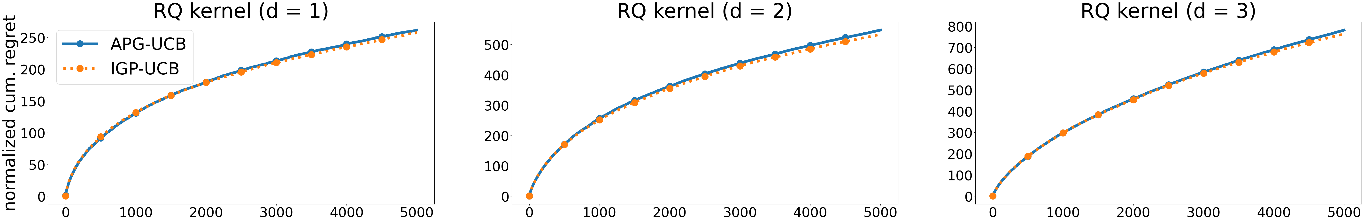
Figure 1: Normalized Cumulative Regret for RQ kernels.

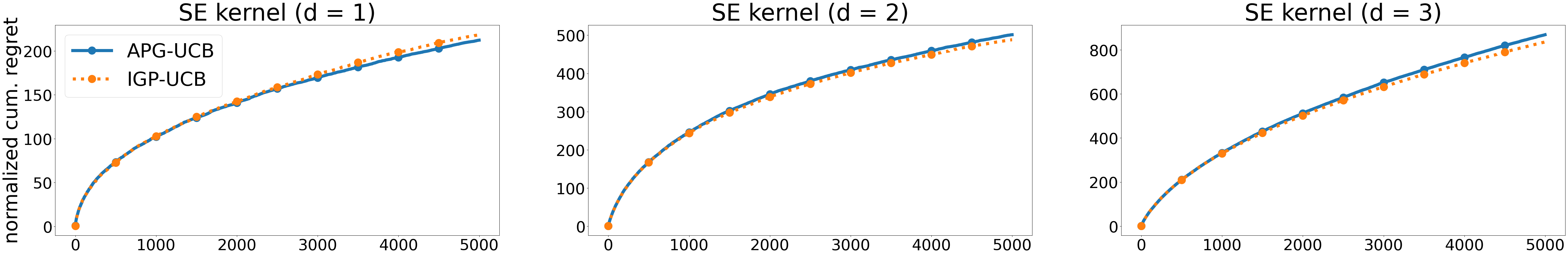
Figure 2: Normalized Cumulative Regret for SE kernels.

7 Discussion

So far, we have emphasized the advantages of our methods. In this section, we discuss limitations of our methods. Here, we focus on Theorem 13 with $q=1/2$ and Theorem 16. Since we do not see limitations if the kernel has infinite smoothness, in this section we assume the kernel is a Matérn kernel. In our theoretical results, $D_{q,\alpha}(T)$ plays a similar role as the information gain in the theoretical result of BBKB. If the kernel is a Matérn kernel with parameter $\nu$, then, by recent results on the information gain (vakili2021information), we have $\gamma_{T}=\widetilde{O}(T^{d/(d+2\nu)})$, which is a nearly optimal result by (Scarlett et al., 2017) and is slightly better than the upper bound of $D_{1/2,\alpha}(T)$. Therefore, in this case the regret upper bound $\widetilde{O}(\sqrt{T}T^{d/(2\nu)})$ of Theorem 13 is slightly worse than the regret upper bound $\widetilde{O}(\sqrt{T}T^{d/(d+2\nu)})$ of BBKB. In addition, similarly SupKernelUCB has nearly optimal regret upper bound if the kernel is Matérn, but regret upper bound of APG-PE is slightly worse in that case.

Inferiority of our method in the Matérn kernel case might be counter-intuitive since it is also proved that the convergence rate of the power function for Matérn kernel is optimal (c.f. Schaback (1995)) and Theorem 9 cannot be improved (Lattimore et al., 2020). We explain why a combination of optimal results leads to a non-optimal result. The results on the information gain depend on the eigenvalue decay of the Mercer operator rather than the decay of the power function in the $L^{\infty}$-norm as in this study. However these two notions are closely related. From the $n$-width theory (Pinkus, 2012, Chapter IV, Corollary 2.6), eigenvalue decay corresponds to the decay of the power function in the $L^{2}$-norm (or more precisely Kolmogorov $n$-width). The decay in the $L^{2}$-norm is derived from that in the $L^{\infty}$-norm. If the kernel is a Matérn kernel, using a localization trick called Duchon’s trick (Wendland, 1997), it can be possible to give a faster decay in the $L^{p}$-norm than that in the $L^{\infty}$-norm if $p<\infty$. Since the norm regarding the misspecified bandit problem is not a $L^{2}$ norm but a $L^{\infty}$ norm, we took the approach proposed in this paper.

8 Experiments

In this section, we empirically verify our theoretical results. We compare APG-UCB to IGP-UCB Chowdhury & Gopalan (2017) in terms of cumulative regret and running time for RQ and SE kernels in synthetic environments.

8.1 Environments

We assume the action set is a discretization of a cube $[0,1]^{d}$ for $d=1,2,3$. We take $\mathcal{A}$ so that $|\mathcal{A}|$ is about $1000$. More precisely, we define $\mathcal{A}$ by $\{i/m_{d}\mid i=0,1,\dots,m_{d}-1\}^{d}$ where $m_{1}=1000,m_{2}=30,m_{3}=10$. We randomly construct reward functions $f\in\mathcal{H}_{K}\left(\Omega\right)$ with $\|f\|_{\mathcal{H}_{K}\left(\Omega\right)}=1$ as follows. We randomly select points $\xi_{i}$ (for $1\leq i\leq m$) from $\mathcal{A}$ until $m\leq 300$ or $\|P_{V(\{\xi_{1},\dots,\xi_{m}\})}\|_{L^{\infty}(\mathcal{A})}<10^{-4}$ and compute orthonormal basis $\{\varphi_{1},\dots,\varphi_{m}\}$ of $V(\{\xi_{1},\dots,\xi_{m}\})$. Then, we define $f=\sum_{i=1}^{m}a_{i}\varphi_{i}$, where $[a_{1},\dots,a_{m}]\in\mathbb{R}^{m}$ is a random vector with unit norm. We take $l=0.3\sqrt{d}$ for the RQ kernel and $l=0.2\sqrt{d}$ for the SE kernel, because the diameter of the $d$-dimensional cube is $\sqrt{d}$. For each kernel, we generate $10$ reward functions as above and evaluate our proposed method and the existing algorithm for time interval $T=5000$ in terms of mean cumulative regret and total running time. We compute the mean of cumulative regret and running time for these 10 environments. We normalize cumulative regret so that normalized cumulative regret of uniform random policy corresponds to the line through origin with slope 1 in the figure. For simplicity, we assume the kernel, $B$, and $R$ are known to the algorithms. For the other parameters, we use theoretically suggested ones for both APG-UCB and IGP-UCB. Computation is done by Intel Xeon E5-2630 v4 processor with 128 GB RAM. In supplementary material, we explain the experiment setting in more detail and provide additional experimental results.

8.2 Results

We show the results for normalized cumulative regret in Figures 1 and 2. As suggested by the theoretical results, growth of the cumulative regret of these algorithms is $\widetilde{O}(\sqrt{T})$ ignoring a polylogarithmic factor. Although, convergence rate of the power function of SE kernels is slightly faster than that of RQ kernels (by remark of Theorem 4), empirical results of RQ kernels and SE kernels are similar. In both cases, APG-UCB has almost the same cumulative regret as that of IGP-UCB.

We also show (mean) total running time in Table 1, where we abbreviate APG-UCB as APG and IGP-UCB as IGP. For all dimensions, it took about from five to six thousand seconds for IGP-UCB to complete an experiment for one environment. As shown by the table and figures, running time of our methods is much shorter than that of IGP-UCB while it has almost the same regret as IGP-UCB.

Table 1: Total Running Time (in seconds).

	APG(RQ)	IGP(RQ)	APG(SE)	IGP(SE)
$d=1$	4.2e-01	5.7e+03	4.0e-01	5.7e+03
$d=2$	2.7e+00	5.1e+03	2.9e+00	5.1e+03
$d=3$	3.0e+01	5.7e+03	4.3e+01	5.7e+03

9 Conclusion

By reducing the RKHS bandit problem to the misspecified linear bandit problem, we provide the first general algorithm for the adversarial RKHS bandit problem and several efficient algorithms for the stochastic RKHS bandit problem. We provide cumulative regret upper bounds for them and empirically verify our theoretical results.

10 Acknowledgement

We would like to thank anonymous reviewers for suggestions that improved the paper. We also would like to thank Janmajay Singh and Takafumi J. Suzuki for valuable comments on the preliminarily version of the manuscript.

Appendix

In this appendix, we provide some results on Thompson Sampling based algorithms in §A, proofs of the results in §B, and detailed experimental setting and additional experimental results in §C.

Appendix A Additional Results for Thompson Sampling

A.1 Misspecified Linear Bandit Problem

We consider a modification of Thompson Sampling (Agrawal & Goyal, 2013). In $(t+1)$th round, we sample $\mu_{t}$ from the multinomial normal distribution $\mathcal{N}\left(\hat{\theta}_{t},\left(\beta(A_{t},\delta/2,\lambda)+\epsilon\psi_{t}\right)^{2}A_{t}^{-1}\right)$, and the modified algorithm selects $x\in\mathcal{A}$ that maximizes $\langle\mu_{t},\widetilde{x}\rangle$. Then the following result holds.

Proposition 18.

We assume that $\lambda\geq 1$. Then, with probability at least $1-\delta$, the modification of Thompson Sampling algorithm incurs regret upper bound by

$$\widetilde{O}\left(\sqrt{\log(|\mathcal{A}|)}\left\{D\sqrt{T}+\sqrt{DT\log(1/\delta)}+\log(1/\delta)\sqrt{T}+\left(DT+T\sqrt{D\log(1/\delta)}\right)\epsilon)\right\}\right)$$

We provide proof of the proposition in §B.4.

A.2 Thompson Sampling for the Stochastic RKHS Bandit Problem

We provide a result on a Thompson Sample based algorithm for the stochastic RKHS bandit problem.

Theorem 19.

We reduce the RKHS bandit problem to the misspecified linear bandit problem, and apply the modified Thompson Sampling introduced above with admissible error $\mathfrak{e}=\frac{\alpha}{T^{q}}$ with $q\geq 1/2$. We denote by $R_{\text{APG-TS}}(T)$ its regret and assume that $\lambda\geq 1$. Then with probability at least $1-\delta$, $R_{\text{APG-TS}}(T)$ is upper bounded by

$$\widetilde{O}\left(\sqrt{\log(|\mathcal{A}|)}\left(D_{q,\alpha}(T)\sqrt{T}+\sqrt{D_{q,\alpha}(T)T\log(1/\delta)}+\log(1/\delta)\sqrt{T})\right)\right).$$

The total computational complexity of the algorithm is given as $O(|\mathcal{A}|TD_{q,\alpha}^{2}(T)+TD_{q,\alpha}^{3}(T))$.

We provide proof of the theorem in §B.5.

Appendix B Proofs

We provide omitted proofs in the main article and §A.

B.1 Proof of Corollary 7

For completeness, we provide a proof of corollary 7.

Proof.

For simplicity, we consider only the infinite smoothness case. We use the same notation as in Theorem 6 and Algorithm 1. Denote by $D$ the number of points returned by the algorithm with error $\mathfrak{e}=\alpha/T^{q}$. Since the statement of the corollary is obvious if $D=1$, we assume $D>1$. Because the condition $\max_{x\in\widehat{\Omega}}P_{m}(x)<\alpha/T^{q}$ is satisfied only when $m\geq D$, we have $\alpha/T^{q}\leq\max_{x\in\widehat{\Omega}}P_{D-1}(x)$. If we run the algorithm with error $\mathfrak{e}=\max_{x\in\widehat{\Omega}}P_{D-1}(x)+\epsilon$ with sufficiently small $\epsilon>0$, then the algorithm returns $D-1$ points. Therefore by the theorem and the inequality above, we have

$$\alpha/T^{q}\leq\max_{x\in\widehat{\Omega}}P_{D-1}(x)<\hat{C_{1}}\exp\left(-\hat{C_{2}}(D-1)^{1/d}\right).$$

Ignoring constants other than $\alpha,T,q$, we have the assertion of the corollary. ∎

B.2 Proof of Proposition 8

For symmetric matrices $P,Q\in\mathbb{R}^{n\times n}$, we write $P\geq Q$ if and only if $P-Q$ is positive semi-definite, i.e., $x^{T}(P-Q)x\geq 0$ for all $x\in\mathbb{R}^{n}$. For completeness, we prove the following elementary lemma.

Lemma 20.

Let $P,Q\in\mathbb{R}^{n\times n}$ be symmetric matrices of size $n$ and assume that $0<P\leq Q$. Then we have $Q^{-1}\leq P^{-1}$.

Proof.

It is enough to prove the statement for $U^{\mathrm{T}}PU$ and $U^{\mathrm{T}}QU$ for some $U\in\mathrm{GL}_{n}(\mathbb{R})$, where $\mathrm{GL}_{n}(\mathbb{R})$ is the general linear group of size $n$. Since $P$ is positive definite, using Cholesky decomposition, one can prove that there exists $U\in\mathrm{GL}_{n}(\mathbb{R})$ such that $U^{\mathrm{T}}PU=1_{n}$ and $U^{\mathrm{T}}QU=\Lambda$ is a diagonal matrix. Then, the assumption implies that every diagonal entry of $\Lambda$ is greater than or equal to $1$. Now, the statement is obvious. ∎

Next, we prove that $\langle\widetilde{x},\theta_{t}\rangle+\|\widetilde{x}\|_{A_{t}^{-1}}(\beta_{t}+\epsilon\psi_{t})$ is a UCB up to a constant.

Lemma 21.

We assume $\lambda\geq 1$. Then, with probability at least $1-\delta$, we have

$$|\langle\widetilde{x},\theta_{t}\rangle-\langle\widetilde{x},\theta\rangle|\leq\|\widetilde{x}\|_{A_{t}^{-1}}(\beta_{t}+\epsilon\psi_{t}),$$

for any $t$ and $\widetilde{x}\in\mathbb{R}^{D}$.

Proof.

By proof of (Abbasi-Yadkori et al., 2011, Theorem 2), we have

$$|\langle\widetilde{x},\theta_{t}\rangle-\langle\widetilde{x},\theta\rangle| \leq\|\widetilde{x}\|_{A_{t}^{-1}}\left(\left\|\sum_{s=1}^{t}\widetilde{x}_{s}(\varepsilon_{s}+\omega(x_{s}))\right\|_{A_{t}^{-1}}+\lambda^{1/2}\|\theta\|\right)$$

$$\leq\|\widetilde{x}\|_{A_{t}^{-1}}\left(\left\|\sum_{s=1}^{t}\widetilde{x}_{s}\varepsilon_{s}\right\|_{A_{t}^{-1}}+\lambda^{1/2}\|\theta\|+\epsilon\sum_{s=1}^{t}\|\widetilde{x}_{s}\|_{A_{t}^{-1}}\right).$$

By the self-normalized concentration inequality (Abbasi-Yadkori et al., 2011), with probability at least $1-\delta$, we have

$$|\langle\widetilde{x},\theta_{t}\rangle-\langle\widetilde{x},\theta\rangle|\leq\|\widetilde{x}\|_{A_{t}^{-1}}\left(\beta_{t}+\epsilon\sum_{s=1}^{t}\|\widetilde{x}_{s}\|_{A_{t}^{-1}}\right).$$

Since $A_{s-1}\leq A_{s}$ for any $s$, by Lemma 20, we have $\sum_{s=1}^{t}\|\widetilde{x}_{s}\|_{A_{t}^{-1}}\leq\psi_{t}$. This completes the proof. ∎

Proof of Proposition 8.

We assume $\lambda\geq 1$. Let $x^{*}:=\operatorname{argmax}_{x\in\mathcal{A}}f(x)$ and $\left(x_{t}\right)_{t}$ be a sequence of arms selected by the algorithm. Denote by $E$ the event on which the inequality in Lemma 21 holds for all $t$ and $\widetilde{x}$. Then on event $E$, we have

$$f(x^{*})-f(x_{t}) \leq 2\epsilon+\langle\widetilde{x}^{*},\theta\rangle-\langle\widetilde{x}_{t},\theta\rangle$$

$$\leq 2\epsilon+\langle\widetilde{x}^{*},\theta_{t}\rangle+\|\widetilde{x}^{*}\|_{A_{t}^{-1}}(\beta_{t}+\epsilon\psi_{t})-\langle\widetilde{x}_{t},\theta\rangle$$

$$\leq 2\epsilon+\langle\widetilde{x}_{t},\theta_{t}\rangle+\|\widetilde{x}_{t}\|_{A_{t}^{-1}}(\beta_{t}+\epsilon\psi_{t})-\left(\langle\widetilde{x}_{t},\theta_{t}\rangle-\|\widetilde{x}_{t}\|_{A_{t}^{-1}}(\beta_{t}+\epsilon\psi_{t})\right)$$

$$=2\epsilon+2\|\widetilde{x}_{t}\|_{A_{t}^{-1}}(\beta_{t}+\epsilon\psi_{t}).$$

Therefore, on event $E$,

$$R(T) \leq 2\epsilon T+2\beta_{T}\sum_{t=1}^{T}\|\widetilde{x}_{t}\|_{A_{t-1}^{-1}}+2\epsilon\sum_{t=1}^{T}\|\widetilde{x}_{t}\|_{A_{t-1}^{-1}}\psi_{t}$$

$$\leq 2\epsilon T+2\beta_{T}\sqrt{T}\sqrt{\sum_{t=1}^{T}\|\widetilde{x}_{t}\|^{2}_{A_{t-1}^{-1}}}+2\epsilon\psi_{T}\sum_{t=1}^{T}\|\widetilde{x}_{t}\|_{A_{t-1}^{-1}}$$

$$=2\epsilon T+2\beta_{T}\sqrt{T}\sqrt{\sum_{t=1}^{T}\|\widetilde{x}_{t}\|^{2}_{A_{t-1}^{-1}}}+2\epsilon\left(\sum_{t=1}^{T}\|\widetilde{x}_{t}\|_{A_{t-1}^{-1}}\right)^{2}$$

$$\leq 2\epsilon T+2\beta_{T}\sqrt{T}\sqrt{\sum_{t=1}^{T}\|\widetilde{x}_{t}\|^{2}_{A_{t-1}^{-1}}}+2\epsilon T\left(\sum_{t=1}^{T}\|\widetilde{x}_{t}\|^{2}_{A_{t-1}^{-1}}\right).$$

By assumptions, we have $\|\widetilde{x}\|_{A_{t-1}^{-1}}\leq\|\widetilde{x}\|_{A_{0}^{-1}}=\lambda^{-1/2}\|\widetilde{x}\|_{2}\leq 1$ for any $x\in\mathcal{A}$. Therefore, by (Abbasi-Yadkori et al., 2011, Lemma 11), the following inequalities hold:

$$\sum_{t=1}^{T}\|\widetilde{x}_{t}\|^{2}_{A_{t-1}^{-1}}\leq 2\log(\det(\lambda^{-1}A_{t}))\leq 2D\log\left(1+\frac{T}{\lambda D}\right),\quad\beta_{t}\leq R\sqrt{D\log\left(1+\frac{T}{\lambda D}\right)+2\log(1/\delta)}+\sqrt{\lambda}B.$$ (1)

Thus, on event $E$, we have

$$R(T) \leq 2\beta_{T}\sqrt{T}\sqrt{2\log(\lambda^{-1}A_{T})}+2\epsilon T+4\epsilon T\log(\det(\lambda^{-1}A_{T}))$$

$$=\widetilde{O}\left(\epsilon T+(\sqrt{D}+\sqrt{1/\delta})\sqrt{DT}+\epsilon DT\right)$$

$$=\widetilde{O}\left(D\sqrt{T}+\sqrt{DT\log(1/\delta)}+\epsilon DT\right).$$

∎

B.3 Proof of Proposition 11

This proposition can be proved by adapting the standard proof of the adversarial linear bandit problem (Lattimore & Szepesvári, 2020; Bubeck & Cesa-Bianchi, 2012). We recall notation for the adversarial misspecified linear bandit problem and EXP3. Let $\mathcal{A}\ni x\mapsto\widetilde{x}\in\{\xi\in\mathbb{R}^{D}:\|\xi\|\leq 1\}$ be a map, $\{g_{t}\}_{t=1}^{T}$ be a sequence of reward functions on $\mathcal{A}$ such that $g_{t}(x)=\langle\theta_{t},\widetilde{x}\rangle+\omega_{t}(x)$ for $x\in\mathcal{A}$, where $\theta_{t}\in\mathbb{R}^{D}$, $\sup_{x\in\mathcal{A}}|g_{t}(x)|,\|\theta_{t}\|\leq B$, and $\sup_{x\in\mathcal{A}}|\omega_{t}(x)|\leq\epsilon$.

Let $\gamma\in(0,1)$ be an exploration parameter, $\eta>0$ a learning rate, and $\pi_{\mathrm{exp}}$ an exploitation distribution over $\mathcal{A}$. For a distribution $\pi$ over $\mathcal{A}$, we put $Q(\pi)=\sum_{x\in\mathcal{A}}\pi(x)\widetilde{x}\widetilde{x}^{\mathrm{T}}$. We define $\phi_{t}=g_{x}(x_{t})Q_{t}^{-1}\widetilde{x}_{t}$ and $\phi_{t}(x)=\langle\phi_{t},\widetilde{x}\rangle$ for $x\in\mathcal{A}$, where the matrix $Q_{t}$ can be computed from the past observations at round $t$ and is defined later. Let $q_{t}$ be a distribution over $\mathcal{A}$ such that $q_{t}(x)\sim\exp\left(\eta\sum_{s=1}^{t-1}\phi_{s}(x)\right)$ and put $p_{t}(x)=\gamma\pi_{\mathrm{exp}}(x)+(1-\gamma)q_{t}(x)$ for $x\in\mathcal{A}$. We assume that $Q(\pi_{\mathrm{exp}})$ is non-singular and define $Q_{t}=Q(p_{t})$. For a distribution $\pi$ over $\mathcal{A}$, we define $\Gamma(\pi)=\sup_{x\in\mathcal{A}}\widetilde{x}^{\mathrm{T}}Q(\pi_{\mathrm{exp}})^{-1}\widetilde{x}$ and in this section we assume $\Gamma(\pi)\leq D$.

Let $x_{*}=\operatorname{argmax}_{x\in\mathcal{A}}\sum_{t=1}^{T}g_{t}(x)$ be an optimal arm and regret is defined as $R(T)=\sum_{t=1}^{T}g_{t}(x_{*})-\sum_{t=1}^{T}g_{t}(x_{t})$. We have

$$\mathbf{E}\left[R(T)\right] =\mathbf{E}\left[\sum_{t=1}^{T}\left(\langle\theta_{t},\widetilde{x}_{*}\rangle-\langle\theta_{t},\widetilde{x}_{t}\rangle\right)\right]+\mathbf{E}\left[\sum_{t=1}^{T}\left(\omega_{t}(\widetilde{x}_{*})-\omega_{t}(\widetilde{x}_{t})\right)\right]$$

$$\leq 2\epsilon T+\mathbf{E}\left[\sum_{t=1}^{T}\left(\langle\theta_{t},\widetilde{x}_{*}\rangle-\langle\theta_{t},\widetilde{x}_{t}\rangle\right)\right].$$ (2)

We denote by $\mathcal{H}_{t-1}$ the sigma field generated by $x_{1},\dots,x_{t-1}$ and by $\mathbf{E}_{t-1}$ the conditional expectation conditioned on $\mathcal{H}_{t-1}$. We note that $p_{t}(x),q_{t}(x)$ for $x\in\mathcal{A}$ and $Q_{t}$ are $\mathcal{H}_{t-1}$-measurable but $\phi_{t}$ is not. Then we have

$$\mathbf{E}\left[\sum_{t=1}^{T}\langle\theta_{t},\widetilde{x}_{t}\rangle\right]=\mathbf{E}\left[\sum_{t=1}^{T}\mathbf{E}_{t-1}\left[\langle\theta_{t},\widetilde{x}_{t}\rangle\right]\right]=\mathbf{E}\left[\sum_{t=1}^{T}\sum_{x\in\mathcal{A}}p_{t}(x){\langle\theta_{t},\widetilde{x}\rangle}\right]$$

$$=\gamma\mathbf{E}\left[\sum_{t=1}^{T}\sum_{x\in\mathcal{A}}{\pi_{\mathrm{exp}}(x)\langle\theta,\widetilde{x}\rangle}\right]+(1-\gamma)\mathbf{E}\left[\sum_{t=1}^{T}\sum_{x\in\mathcal{A}}{q_{t}(x)\langle\theta_{t},\widetilde{x}\rangle}\right]$$

$$\geq-\gamma BT+(1-\gamma)S.$$ (3)

Here we used $|\langle\theta_{t},\widetilde{x}\rangle|\leq\|\theta_{t}\|\|\widetilde{x}\|\leq B$ and $S$ is defined as $\mathbf{E}\left[\sum_{t=1}^{T}\sum_{x\in\mathcal{A}}{q_{t}(x)\langle\theta_{t},\widetilde{x}\rangle}\right]$. Since $\sum_{t=1}^{T}\langle\theta_{t},\widetilde{x}_{*}\rangle\leq\gamma BT+(1-\gamma)\sum_{t=1}^{T}\langle\theta_{t},\widetilde{x}_{*}\rangle$, by inequalities (2), (3), we have

$$\mathbf{E}\left[R(T)\right]\leq 2\epsilon T+2\gamma BT+(1-\gamma)\left(\sum_{t=1}^{T}\langle\theta_{t},\widetilde{x}_{*}\rangle-S\right).$$ (4)

We decompose $S=S_{1}+S_{2}$, where

$$S_{1}=\mathbf{E}\left[\sum_{t=1}^{T}\sum_{x\in\mathcal{A}}{q_{t}(x)\langle\phi_{t},\widetilde{x}\rangle}\right],\quad S_{2}=\mathbf{E}\left[\sum_{t=1}^{T}\sum_{x\in\mathcal{A}}{q_{t}(x)\langle\theta_{t}-\phi_{t},\widetilde{x}\rangle}\right].$$

First, we bound $|S_{2}|$. To do this, we prove the following lemma.

Lemma 22.

For any $x\in\mathcal{A}$, the following inequality holds:

$$\left|\mathbf{E}_{t-1}\left[\langle\phi_{t}-\theta_{t},\widetilde{x}\rangle\right]\right|\leq\frac{\epsilon\Gamma(\pi_{\mathrm{exp}})}{\gamma}.$$

In particular, we have $\left|\mathbf{E}\left[\langle\phi_{t}-\theta_{t},\widetilde{x}\rangle\right]\right|\leq\frac{\epsilon\Gamma(\pi_{\mathrm{exp}})}{\gamma}$.

Proof.

We note that by conditioning on $\mathcal{H}_{t-1}$, randomness comes only from $x_{t}$. By definition of $\phi_{t}$, we have

$$\mathbf{E}_{t-1}\left[\langle\phi_{t},\widetilde{x}\rangle\right] =\mathbf{E}_{t-1}\left[\langle\left(\langle\theta_{t},\widetilde{x}_{t}\rangle+\omega_{t}(x_{t})\right)Q_{t}^{-1}\widetilde{x}_{t},\widetilde{x}\rangle\right]$$

$$=\mathbf{E}_{t-1}\left[\widetilde{x}^{\mathrm{T}}Q_{t}^{-1}\widetilde{x}_{t}\widetilde{x}_{t}^{\mathrm{T}}\theta_{t}\right]+\mathbf{E}_{t-1}\left[\omega_{t}(x_{t})\widetilde{x}^{\mathrm{T}}Q_{t}^{-1}\widetilde{x}_{t}\right]$$

$$=\langle\theta_{t},\widetilde{x}\rangle+\mathbf{E}_{t-1}\left[\omega_{t}(x_{t})\widetilde{x}^{\mathrm{T}}Q_{t}^{-1}\widetilde{x}_{t}\right].$$

Therefore,

$$\left|\mathbf{E}_{t-1}\left[\langle\phi_{t}-\theta_{t},\widetilde{x}\rangle\right]\right|\leq\epsilon\mathbf{E}_{t-1}\left[\|\widetilde{x}_{t}\|_{Q_{t}^{-1}}\|\widetilde{x}\|_{Q_{t}^{-1}}\right]\leq\frac{\epsilon}{\gamma}\mathbf{E}_{t-1}\left[\|\widetilde{x}_{t}\|_{Q(\pi_{\mathrm{exp}})^{-1}}\|\widetilde{x}\|_{Q(\pi_{\mathrm{exp}})^{-1}}\right]\leq\frac{\epsilon\Gamma(\pi_{\mathrm{exp}})}{\gamma}.$$

Here in the second inequality, we use $\gamma Q(\pi_{\mathrm{exp}})\leq Q_{t}$ and the last inequality follows from the definition of $\Gamma(\pi_{\mathrm{exp}})$. The second assertion follows from

$$\left|\mathbf{E}\left[\langle\phi_{t}-\theta_{t},\widetilde{x}\rangle\right]\right|\leq\mathbf{E}\left[\left|\mathbf{E}_{t-1}\left[\langle\phi_{t}-\theta_{t},\widetilde{x}\rangle\right]\right|\right]\leq\frac{\epsilon\Gamma(\pi_{\mathrm{exp}})}{\gamma}.$$

∎

By this lemma, we can bound $S_{2}$ as follows.

Lemma 23.

The following inequality holds:

$$|S_{2}|\leq\frac{\epsilon T\Gamma(\pi_{\mathrm{exp}})}{\gamma}.$$

Proof.

Since $q_{t}(x)$ is $\mathcal{H}_{t-1}$-measurable for any $x\in\mathcal{A}$, we have

$$S_{2}=\mathbf{E}\left[\sum_{t=1}^{T}\sum_{x\in\mathcal{A}}q_{t}(x)\mathbf{E}_{t-1}\left[\langle\theta_{t}-\phi_{t},\widetilde{x}\rangle\right]\right].$$

Therefore, we have

$$|S_{2}|\leq\mathbf{E}\left[\sum_{t=1}^{T}\sum_{x\in\mathcal{A}}q_{t}(x)\left|\mathbf{E}_{t-1}\left[\langle\theta_{t}-\phi_{t},\widetilde{x}\rangle\right]\right|\right]\leq\frac{\epsilon T\Gamma(\pi_{\mathrm{exp}})}{\gamma}.$$

Here we used Lemma 22 in the last inequality. ∎

Next, we introduce the following elementary lemma (c.f. Chatterji et al. (2019, Lemma 49)).

Lemma 24.

Let $\eta>0$ and $X$ be a random variable. We assume that $\eta X\leq 1$ almost surely. Then we have

$$\mathbf{E}\left[X\right]\geq\frac{1}{\eta}\log\left(\mathbf{E}\left[\exp(\eta X)\right]\right)-(e-2)\eta\mathbf{E}\left[X^{2}\right].$$

Proof.

By $\log(x)\leq x-1$ for $x>0$ and $\exp(y)\leq 1+y+(e-2)y^{2}$ for $y\leq 1$, we have

$$\log\mathbf{E}\left[\exp(\eta X)\right]\leq\mathbf{E}\left[\exp(\eta X)\right]-1\leq\mathbf{E}\left[\eta X+(e-2)\eta^{2}X^{2}\right].$$

∎

To apply the lemma with $X=\langle\phi_{t},\widetilde{x}\rangle$ and $\mathbf{E}=\mathbf{E}_{x\sim q_{t}}$, we prove the following:

Lemma 25.

Let $x\in\mathcal{A}$ and assume that $\gamma=\eta B\Gamma(\pi_{\mathrm{exp}})$. Then, we have $\eta|\langle\phi_{t},\widetilde{x}\rangle|\leq 1$.

Proof.

By definition of $\phi_{t}$, we have

$$\eta|g_{t}(x_{t})\widetilde{x}_{t}^{\mathrm{T}}Q_{t}^{-1}\widetilde{x}|\leq\eta B\|\widetilde{x}_{t}\|_{Q_{t}^{-1}}\|\widetilde{x}\|_{Q_{t}^{-1}}\leq\frac{\eta B\Gamma(\pi_{\mathrm{exp}})}{\gamma}.$$

Here, in the last inequality, we use $\gamma Q(\pi_{\mathrm{exp}})\leq Q_{t}$ and the definition of $\Gamma(\pi_{\mathrm{exp}})$. ∎

By Lemma 24 and Lemma 25, we obtain the following.

$$S_{1}\geq\frac{U_{1}}{\eta}-(e-2)\eta U_{2},$$ (5)

where $U_{1}$ and $U_{2}$ are given as

$$U_{1}=\mathbf{E}\left[\sum_{t=1}^{T}\log\left(\sum_{x\in\mathcal{A}}{q_{t}(x)\exp\left(\eta\langle\phi_{t},\widetilde{x}\rangle\right)}\right)\right],\quad U_{2}=\mathbf{E}\left[\sum_{t=1}^{T}\sum_{x\in\mathcal{A}}{q_{t}(x)\langle\phi_{t},\widetilde{x}\rangle^{2}}\right].$$

We bound $|U_{2}|$ as follows.

Lemma 26.

The following inequality holds:

$$|U_{2}|\leq\frac{B^{2}DT}{1-\gamma}.$$

Proof.

By definition of $\phi_{t}$, we have

$$\sum_{x\in\mathcal{A}}q_{t}(x)\langle\phi_{t},\widetilde{x}\rangle^{2}\leq B^{2}\sum_{x\in\mathcal{A}}q_{t}(x)\widetilde{x}_{t}^{\mathrm{T}}Q_{t}^{-1}\widetilde{x}\widetilde{x}^{\mathrm{T}}Q_{t}^{-1}\widetilde{x}_{t}=B^{2}\widetilde{x}_{t}Q_{t}^{-1}Q(q_{t})Q_{t}^{-1}\widetilde{x}_{t}$$

$$\leq\frac{B^{2}}{1-\gamma}\widetilde{x}_{t}^{\mathrm{T}}Q_{t}^{-1}\widetilde{x}_{t}.$$

Here the last inequality follows from $(1-\gamma)Q(q_{t})\leq Q_{t}$. Therefore,

$$\mathbf{E}\left[\sum_{x\in\mathcal{A}}\langle\phi_{t},\widetilde{x}\rangle^{2}\right]\leq\frac{B^{2}}{1-\gamma}\mathbf{E}\left[\widetilde{x}_{t}^{\mathrm{T}}Q_{t}^{-1}\widetilde{x}_{t}\right]=\frac{B^{2}}{1-\gamma}\mathbf{E}\left[\operatorname{Tr}\left(\widetilde{x}_{t}\widetilde{x}_{t}^{\mathrm{T}}Q_{t}^{-1}\right)\right]$$

$$=\frac{B^{2}}{1-\gamma}\mathbf{E}\left[\operatorname{Tr}\left(Q_{t}Q_{t}^{-1}\right)\right]=\frac{B^{2}D}{1-\gamma}.$$

Here the second equality follows from the fact that $Q_{t}$ is $\mathcal{H}_{t-1}$-measurable and the linearity of the trace. The assertion of the lemma follows from this. ∎

Next, we give a lower bound for $U_{1}$.

Lemma 27.

Let $x_{0}\in\mathcal{A}$ be any element. Then the following inequality holds:

$$U_{1}\geq\eta\mathbf{E}\left[\sum_{t=1}^{T}\langle\phi_{t},\widetilde{x}_{0}\rangle\right]-\log(|\mathcal{A}|).$$

Proof.

By definition of $q_{t}$, we have

$$U_{1} =\mathbf{E}\left[\sum_{t=1}^{T}\left\{\log\left(\sum_{x\in\mathcal{A}}\exp\left(\eta\sum_{s=1}^{t}\langle\phi_{s},\widetilde{x}\rangle\right)\right)-\log\left(\sum_{x\in\mathcal{A}}\exp\left(\eta\sum_{s=1}^{t-1}\langle\phi_{s},\widetilde{x}\rangle\right)\right)\right\}\right]$$

$$=\mathbf{E}\left[\log\left(\sum_{x\in\mathcal{A}}\exp\left(\eta\sum_{s=1}^{T}\langle\phi_{s},\widetilde{x}\rangle\right)\right)\right]-\log|\mathcal{A}|$$

$$=\eta\mathbf{E}\left[\sum_{t=1}^{T}\langle\phi_{t},\widetilde{x}_{0}\rangle\right]-\log|\mathcal{A}|.$$

∎

Proof of Proposition 11.

We assume $\gamma=\eta B\Gamma(\pi_{\mathrm{exp}})$. By (4), we have

$$\mathbf{E}\left[R(T)\right]\leq 2\epsilon T+2\gamma BT+(1-\gamma)\mathbf{E}\left[\sum_{t=1}^{T}\langle\theta_{t},\widetilde{x}_{*}\rangle\right]-(1-\gamma)S_{1}+(1-\gamma)|S_{2}|$$

By inequality (5), Lemma 23, and Lemma 27 with $x_{0}=x_{*}$, we have

$$\mathbf{E}\left[R(T)\right]\leq 2\epsilon T+2\gamma BT+(1-\gamma)\mathbf{E}\left[\sum_{t=1}^{T}\langle\theta_{t}-\phi_{t},\widetilde{x}_{*}\rangle\right]+\frac{1-\gamma}{\eta}\log|\mathcal{A}|+(e-2)\eta(1-\gamma)U_{2}+\frac{\epsilon T\Gamma(\pi_{\mathrm{exp}})}{\gamma}$$

$$\leq 2\epsilon T+2\gamma BT+\frac{\epsilon T\Gamma(\pi_{\mathrm{exp}})(1-\gamma)}{\gamma}+\frac{\log|\mathcal{A}|}{\eta}+(e-2)\eta B^{2}DT+\frac{\epsilon T\Gamma(\pi_{\mathrm{exp}})}{\gamma}$$

$$\leq 2\epsilon T+2\gamma BT+\frac{\log|\mathcal{A}|}{\eta}+(e-2)\eta B^{2}DT+\frac{2\epsilon T\Gamma(\pi_{\mathrm{exp}})}{\gamma}.$$

Here in the second inequality, we used Lemma 22 and Lemma 26. By $\gamma=\eta B\Gamma(\pi_{\mathrm{exp}})$ and $\Gamma(\pi_{\mathrm{exp}})\leq D$, we have

$$\mathbf{E}\left[R(T)\right]\leq 2\epsilon T+2B^{2}\eta T\Gamma(\pi_{\mathrm{exp}})+\frac{2\epsilon T}{B\eta}+\frac{\log|\mathcal{A}|}{\eta}+(e-2)B^{2}\eta DT$$

$$\leq 2\epsilon T+eB^{2}\eta DT+\frac{2\epsilon T}{B\eta}+\frac{\log|\mathcal{A}|}{\eta}.$$

∎

B.4 Proof of Proposition 18

We assume $\lambda\geq 1$. This can be proved by modifying the proof of (Agrawal & Goyal, 2013). Since most of their arguments can be directly applicable to our case, we omit proofs of some lemmas. Let $(\Psi,\operatorname{Pr},\mathcal{G})$ be the probability space on which all random variables considered here are defined, where $\mathcal{G}\subset 2^{\Psi}$ is a $\sigma$-algebra on $\Psi$. We put $x^{*}:=\operatorname{argmax}_{x\in\mathcal{A}}g(x)$ and for $t=1,2,\dots,T$ and $x\in\mathcal{A}$, we put $\Delta(x):=\langle\widetilde{x}^{*},\theta\rangle-\langle\widetilde{x},\theta\rangle$. We also put $v_{t}:=l_{t}:=\beta(A_{t-1},\delta/(2T),\lambda)+\epsilon\psi_{t-1}$ and $g_{t}:=\sqrt{4\log(|\mathcal{A}|t)}v_{t}+l_{t}$. In each round $t$, $\mu_{t-1}$ is sampled from the multinomial normal distribution $\mathcal{N}\left(\theta_{t-1},\left(\beta(A_{t-1},\delta/2,\lambda)+\epsilon\psi_{t}\right)^{2}A_{t-1}^{-1}\right)$. For $t=1,\dots,T$, we define $E_{t}$ by

$$E_{t}:=\left\{\psi\in\Psi:|\langle\widetilde{x},\theta_{t-1}\rangle-\langle\widetilde{x},\theta\rangle|\leq l_{t}\|\widetilde{x}\|_{A_{t-1}^{-1}},\quad\forall x\in\mathcal{A}\right\},$$

and define event $E^{\prime}_{t}$ by

$$E_{t}^{\prime}:=\left\{\psi\in\Psi:|\langle\widetilde{x},\mu_{t-1}\rangle-\langle\widetilde{x},\theta_{t-1}\rangle|\leq\sqrt{4\log(|\mathcal{A}|t)}v_{t}\|\widetilde{x}\|_{A_{t-1}^{-1}},\quad\forall x\in\mathcal{A}\right\}.$$

For an event $G$, we denote by $1_{G}$ the corresponding indicator function. Then by assumptions, we see that $E_{t}\in\mathcal{F}_{t-1}$, i.e., $1_{E_{t}}$ is $\mathcal{F}_{t-1}$-measurable. For a random variable $X$ on $\Psi$, we say “on event $E_{t}$, the conditional expectation (or conditional probability) $\mathbf{E}\left[X\mid\mathcal{F}_{t-1}\right]$ satisfies a property” if and only if $1_{E_{t}}\mathbf{E}\left[X\mid\mathcal{F}_{t-1}\right]=\mathbf{E}\left[1_{E_{t}}X\mid\mathcal{F}_{t-1}\right]$ satisfies the property for almost all $\psi\in\Psi$.

Then by Lemma 21 and the proof of (Agrawal & Goyal, 2013, Lemma 1), we have

Lemma 28.

$\operatorname{Pr}(E_{t})\geq 1-\frac{\delta}{2T}$ and $\operatorname{Pr}(E^{\prime}_{t}\mid\mathcal{F}_{t-1})\geq 1-1/t^{2}$ for all $t$.

We note that the proof of (Agrawal & Goyal, 2013, Lemma 2) works if $l_{t}\leq v_{t}$, i.e., we have the following lemma:

Lemma 29.

On event $E_{t}$, we have

$$\operatorname{Pr}\left(\langle\mu_{t},\widetilde{x}^{*}\rangle>\langle\theta,\widetilde{x}^{*}\rangle\mid\mathcal{F}_{t-1}\right)\geq p,$$

where $p=\frac{1}{4e\sqrt{\pi}}$.

The main differences of our proof and theirs lie in the definitions of $l_{t},v_{t},x^{*}$, and $\Delta(x)$ (they define $\Delta(x)$ as $\sup_{y\in\mathcal{A}}\langle\theta,\widetilde{y}\rangle-\langle\theta,\widetilde{x}\rangle$ and we consider $x^{*}=\operatorname{argmax}g(x)$ instead of $\operatorname{argmax}_{x}\langle\widetilde{x},\theta\rangle$). However, it can be verified that these differences do not matter in the arguments of Lemma 3, 4 in (Agrawal & Goyal, 2013). In fact, we can prove the following lemma in a similar way to the proof of (Agrawal & Goyal, 2013, Lemma 3).

Lemma 30.

We define $C(t)$ by $\{x\in\mathcal{A}:\Delta(x)>g_{t}\|\widetilde{x}\|_{A_{t-1}^{-1}}\}$. On event $E_{t}$, we have

$$\operatorname{Pr}(x\not\in C(t)\mid\mathcal{F}_{t-1})\geq p-\frac{1}{t^{2}}.$$

Here $p$ is given in Lemma 29.

Proof.

Because the algorithm selects $x\in\mathcal{A}$ that maximizes $\langle\widetilde{x},\mu_{t-1}\rangle$, if $\langle\widetilde{x}^{*},\mu_{t-1}\rangle>\langle\widetilde{x},\mu_{t-1}\rangle$ for all $x\in C(t)$, then we have $x_{t}\not\in C(t)$. Therefore, we have

$$\operatorname{Pr}(x_{t}\not\in C(t)\mid\mathcal{F}_{t-1})\geq\operatorname{Pr}\left(\langle\widetilde{x}^{*},\mu_{t-1}\rangle>\langle\widetilde{x},\mu_{t-1}\rangle,\forall x\in C(t)\mid\mathcal{F}_{t-1}\right).$$ (6)

By definitions of $C(t),E_{t}$, and $E_{t}^{\prime}$, on even $E_{t}\cap E_{t}^{\prime}$, we have $\langle\widetilde{x},\mu_{t-1}\rangle\leq\langle\widetilde{x},\theta\rangle+g_{t}\|\widetilde{x}\|_{A_{t-1}^{-1}}<\langle\widetilde{x}^{*},\theta\rangle$ for all $x\in C(t)$. Therefore, on $E_{t}\cap E_{t}^{\prime}$, if $\langle\widetilde{x}^{*},\mu_{t-1}\rangle>\langle\widetilde{x}^{*},\theta\rangle$, we have $\langle\widetilde{x}^{*},\mu_{t-1}\rangle>\langle\widetilde{x},\mu_{t-1}\rangle$ for all $x\in C(t)$. Thus we obtain the following inequalities:

$$\operatorname{Pr}(\langle\widetilde{x}^{*},\mu_{t-1}\rangle>\langle\widetilde{x},\mu_{t-1}\rangle,\quad\forall x\in C(t)\mid\mathcal{F}_{t-1})$$

$$\geq\operatorname{Pr}(\langle\widetilde{x}^{*},\mu_{t-1}\rangle>\langle\widetilde{x}^{*},\theta\rangle\mid\mathcal{F}_{t-1})-\operatorname{Pr}((E_{t}^{\prime})^{c}\mid\mathcal{F}_{t-1})$$

$$\geq p-1/t^{2}.$$

Here $(E_{t}^{\prime})^{c}$ is the complement of $E_{t}^{\prime}$ and we used Lemmas 28, 29 in the last inequality. By inequality (6), we have our assertion. ∎

We can also prove the following lemma in a similar way to the proof of (Agrawal & Goyal, 2013, Lemma 4).

Lemma 31.

On event $E_{t}$, we have

$$\mathbf{E}\left[\Delta(x_{t})\mid\mathcal{F}_{t-1}\right]\leq c_{1}g_{t}\mathbf{E}\left[\|x_{t}\|_{A_{t-1}^{-1}}\mid\mathcal{F}_{t-1}\right]+\frac{c_{2}g_{t}}{t^{2}},$$

where $c_{1}$ and $c_{2}$ are universal constants.

For $t=1,2,\dots,T$, define random variables $X_{t}$ and $Y_{t}$ by

$$X_{t}:=\Delta(x_{t})1_{E_{t}}-c_{1}g_{t}\|x_{t}\|_{A_{t-1}^{-1}}-\frac{c_{2}g_{t}}{t^{2}},\quad Y_{t}:=\sum_{s=1}^{t}X_{t}.$$

From Lemma 31, we can prove the following lemma.

Lemma 32.

The process $\{Y_{t}\}_{t=0,\dots,T}$ is a super-martingale process w.r.t. the filtration $\{\mathcal{F}_{t}\}_{t}$.

Proof of Proposition 18.

By Lemma 32 and $\|X_{t}\|\leq 2(B+\epsilon)+(c_{1}+c_{2})g_{t}$ (for all $t$), applying Azuma-Hoeffding inequality, we see that there exists an event $G$ with $\operatorname{Pr}(G)\geq 1-\delta/2$ such that on $G$, the following inequality holds:

$$\sum_{t=1}^{T}\Delta(x_{t})1_{E_{t}}\leq\sum_{t=1}^{T}c_{1}g_{t}\|\widetilde{x}_{t}\|_{A_{t-1}^{-1}}+\sum_{t=1}^{T}c_{2}g_{t}/t^{2}+\sqrt{\left(4T(B+\epsilon)^{2}+2(c_{1}+c_{2})^{2}\sum_{t=1}^{T}g_{t}^{2}\right)\log(2/\delta)}.$$

Since $g_{t}\leq g_{T}$ for any $t$, on the event $G$, we have

$$\sum_{t=1}^{T}\Delta(x_{t})1_{E_{t}}\leq c_{1}g_{T}\sqrt{T}\sqrt{\sum_{t=1}^{T}\|\widetilde{x}_{t}\|^{2}_{A_{t-1}^{-1}}}+c_{2}g_{T}\frac{\pi^{2}}{6}+\sqrt{T}\sqrt{\left(4(B+\epsilon)^{2}+2(c_{1}+c_{2})^{2}g_{T}^{2}\right)\log(2/\delta)}.$$

By inequalities (1), we have

$$\sqrt{\sum_{t=1}^{T}\|\widetilde{x}_{t}\|^{2}_{A_{t-1}^{-1}}} =\widetilde{O}(\sqrt{D}),\quad g_{T}=\widetilde{O}(\sqrt{\log(|\mathcal{A}|)}v_{T})=\widetilde{O}\left(\sqrt{|\log|\mathcal{A}|}(\sqrt{D}+\sqrt{\log(1/\delta)}+\epsilon\psi_{T})\right).$$

Since $\psi_{T}=\sum_{s=1}^{T}\|\widetilde{x}_{s}\|_{A_{s-1}^{-1}}\leq\sqrt{T}\sqrt{\sum_{s=1}^{T}\|\widetilde{x}_{s}\|^{2}_{A_{s-1}^{-1}}}=\widetilde{O}(\sqrt{DT})$, we obtain

$$g_{T}=\widetilde{O}\left(\sqrt{\log A}(\sqrt{D}+\sqrt{\log(1/\delta)}+\epsilon\sqrt{DT})\right).$$

Therefore, on the event $G$, we have

$$\sum_{t=1}^{T}\Delta(x_{t})1_{E_{t}}=\widetilde{O}\left(\sqrt{\log(|\mathcal{A}|)}\left\{D\sqrt{T}+\sqrt{DT\log(1/\delta)}+\log(1/\delta)\sqrt{T}+\left(DT+T\sqrt{D\log(1/\delta)}\right)\epsilon)\right\}\right).$$

Therefore, on event $\bigcap_{t=1}^{T}E_{t}\cap G$, we can upper bound the regret as follows:

$$R(T) =\sum_{t=1}^{T}\{g(x^{*})-g(x_{t})\}\leq\epsilon T+\sum_{t=1}^{T}\Delta(x_{t})1_{E_{t}}$$

$$=\widetilde{O}\left(\sqrt{\log(|\mathcal{A}|)}\left\{D\sqrt{T}+\sqrt{DT\log(1/\delta)}+\log(1/\delta)\sqrt{T}+\left(DT+T\sqrt{D\log(1/\delta)}\right)\epsilon)\right\}\right).$$

Since $\operatorname{Pr}(\bigcap_{t=1}^{T}E_{t}\cap G)\geq 1-\delta$, we have the assertion of the proposition. ∎

B.5 Proof of Theorem 13

Since Theorems 16, 19 can be proved in a similar way, we only provide proof of Theorem 13.

Let $\{\xi_{1},\dots,\xi_{D}\}$ and $N_{1},\dots,N_{D}$ be a sequence of points and Newton basis returned by Algorithm 2 with $\mathfrak{e}=\frac{\alpha}{T^{q}}$, where $D=D_{q,\alpha}(T)$ and $q\geq 1/2$.

We verify the assumptions of the (stochastic) misspecified linear bandit problem hold, i.e., we show there exists $\theta\in\mathbb{R}^{D}$ such that the following conditions are satisfied for $\widetilde{x}=[N_{1}(x),\dots,N_{D}(x)]^{\mathrm{T}}$ and $\theta$:

1. $\|\widetilde{x}\|_{2}\leq 1$.

2. If $x$ is a $\mathcal{A}$-valued random variable and $\mathcal{F}_{t}$-measurable, then $\widetilde{x}$ is $\mathcal{F}_{t}$-measurable .

3. $\|\theta\|_{2}\leq B$.

4. $\sup_{x\in\mathcal{A}}|f(x)-\langle\theta,\widetilde{x}\rangle|<\epsilon$, where $\epsilon=\alpha B/T^{q}$.

We put $X_{D}:=\{\xi_{1},\dots,\xi_{D}\}$. Then by definition, Newton basis $N_{1},\dots,N_{D}$ is a basis of $V(X_{D})$. We define $\theta_{1},\dots,\theta_{D}\in\mathbb{R}$ by $\Pi_{V(X_{D})}f=\sum_{i=1}^{D}\theta_{i}N_{i}$ and put $\theta=[\theta_{1},\dots,\theta_{D}]^{\mathrm{T}}$. Since Newton basis is an orthonormal basis of $V(X_{D})$, we have

$$\|\theta\|_{2}=\left\|\sum_{i=1}^{D}\theta_{i}N_{i}\right\|_{\mathcal{H}_{K}\left(\Omega\right)}=\left\|\Pi_{V(X_{D})}f\right\|_{\mathcal{H}_{K}\left(\Omega\right)}\leq\|f\|_{\mathcal{H}_{K}\left(\Omega\right)}\leq B.$$

By the orthonormality, we have $P_{V(X)}^{2}(x)=K(x,x)-\sum_{i=1}^{m}N_{i}^{2}(x)$ (c.f. Santin & Haasdonk (2017, Lemma 5)). Then by assumption, we have $\|\widetilde{x}\|_{2}^{2}=\sum_{i=1}^{m}N_{i}^{2}(x)=K(x,x)-P_{V(X_{D})}^{2}(x)\leq 1$. Since $N_{k}$ for $k=1,\dots,D$ is a linear combination of $K(\cdot,\xi_{1}),\dots,K(\cdot,\xi_{D})$ and $K$ is continuous, $x\mapsto\widetilde{x}$ is continuous. Therefore, $\widetilde{x}$ is $\mathcal{F}_{t}$-measurable if $x$ is $\mathcal{F}_{t}$-measurable. By definition of the P-greedy algorithm, we have $\sup_{x\in\mathcal{A}}P_{V(X_{D})}(x)<\frac{\alpha}{T^{q}}$. By this inequality and the definition of the power function, the following inequality holds:

$$\sup_{x\in\mathcal{A}}|f(x)-\langle\theta,\widetilde{x}\rangle|=\sup_{x\in\mathcal{A}}|f(x)-\left(\Pi_{V(X_{D})}f\right)(x)|\leq\|f\|\frac{\alpha}{T^{q}}\leq\frac{\alpha B}{T^{q}}.$$

Thus, one can apply results of a misspecified linear bandit problem with $\epsilon=\frac{\alpha B}{T^{q}}$. By applying Proposition 8, with probability at least $1-\delta$, the regret is upper bounded as follows:

$$R_{\text{APG-UCB}}(T)=\widetilde{O}\left(\sqrt{TD_{q,\alpha}(T)\log(1/\delta)}+D_{q,\alpha}(T)\sqrt{T}\right).$$

Since computing Newton basis requires $O(|\mathcal{A}|D^{2})$ time and total complexity of the modified LinUCB is given as $O(|\mathcal{A}|D^{2}T)$, we have the assertion of Theorem 13.

B.6 Proof of Theorem 17

For simplicity, by normalization, we assume $B=1$. We denote by $R_{\text{APG-EXP3{}}}(T)$ the cumulative regret that APG-EXP3 with $q=1$ and $\alpha=\log(|\mathcal{A}|)$ incurs up to time step $T$. We can reduce the adversarial RKHS bandit problem to the adversarial misspecified linear bandit problem as in §B.5. To apply Proposition 11, we need to prove that $\{\widetilde{x}|x\in\mathcal{A}\}$ spans $\mathbb{R}^{D}$. We denote by $X=\{X_{1},\dots,X_{D}\}$ the points returned by the $P$-greedy algorithm. Then, since $N_{1},\dots,N_{D}$ is a basis of $V(X)$ and $K$ is positive definite, $\mathrm{rank}\hskip 2.0pt(N_{i}(x))_{1\leq i\leq D,x\in\mathcal{A}}=\mathrm{rank}\hskip 2.0pt(K(x_{i},x))_{1\leq i\leq D,x\in\mathcal{A}}=D$. Therefore, $\{\widetilde{x}|x\in\mathcal{A}\}$ spans $\mathbb{R}^{D}$.

By Proposition 11, we have

$$\mathbf{E}\left[R_{\text{APG-EXP3{}}}(T)\right]\leq 2\epsilon T+e\eta DT+\frac{2\epsilon}{\eta}+\frac{\log(|\mathcal{A}|)}{\eta},$$

where $\epsilon=\frac{\log(|\mathcal{A}|)}{T}$ and $D=D_{1,\log(|\mathcal{A}|)}(T)$. Thus we have $\mathbf{E}\left[R_{\text{APG-EXP3{}}}(T)\right]\leq 2\log(|\mathcal{A}|)+e\eta DT+\frac{3\log(|\mathcal{A}|)}{\eta}.$ By taking $\eta=\sqrt{\frac{\log(|\mathcal{A}|)}{DT}}$, we have the assertion of the theorem.

B.7 Proof of Theorem 14

First, we prove that the $P$-greedy algorithm (Algorithm 1) also gives a uniform kernel approximation.

Lemma 33.

Let $N_{1},\dots,N_{D}$ be a Newton basis returned by the $P$-greedy algorithm 1 with error $\mathfrak{e}$ and $\widehat{\Omega}=\mathcal{A}$. For $x\in\mathcal{A}$, we put $\widetilde{x}:=[N_{1}(x),\dots,N_{D}(x)]^{\mathrm{T}}$. Then, we have $\sup_{x,y\in\mathcal{A}}|K(x,y)-\langle\widetilde{x},\widetilde{y}\rangle|\leq\mathfrak{e}.$

Proof.

We denote by $X$ the points returned by the $P$-greedy algorithm. Then, by definition of the Power function, we have

$$\left|h(x)-\left(\Pi_{V(X)}h\right)(x)\right|\leq\|h\|_{\mathcal{H}_{K}\left(\Omega\right)}\mathfrak{e},$$

for any $h\in\mathcal{H}_{K}\left(\Omega\right)$ and $x\in\mathcal{A}$. We take arbitrary $y\in\mathcal{A}$ and take $h=K(\cdot,y)$. Since $N_{1},\dots,N_{D}$ is an orthonormal basis of $V(X)$, we have

$$\left(\Pi_{V(X)}h\right)(x)=\sum_{i=1}^{D}\langle h,N_{i}\rangle_{\mathcal{H}_{K}\left(\Omega\right)}N_{i}(x)=\sum_{i=1}^{D}N_{i}(y)N_{i}(x)=\langle\widetilde{x},\widetilde{y}\rangle.$$

Here, in the second equality, we used the reproducing property. Since $\|h\|_{\mathcal{H}_{K}\left(\Omega\right)}\leq 1$ and $x,y$ are arbitrary, we have our assertion. ∎

Next, we introduce the following classical result on matrix eigenvalues.

Lemma 34 (a specail case of the Wielandt-Hoffman theorem Hoffman et al. (1953)).

Let $A,B\in\mathbb{R}^{n\times n}$ be symmetric matrices. Denote by $a_{1}\leq\dots\leq a_{n}$ and $b_{1}\leq\dots\leq b_{n}$ be the eigenvalues of $A$ and $B$ respectively. Then, we have $\sum_{i=1}^{n}|a_{i}-b_{i}|^{2}\leq\|A-B\|_{F}^{2},$ where $\|\cdot\|_{F}$ denotes the Frobenius norm.

By these lemmas, we can prove $\log\det\left(\lambda^{-1}A_{T}\right)$ is an approximation of the maximum information gain.

Lemma 35.

We apply APG-UCB with admissible error $\mathfrak{e}$ to the stochastic RKHS bandit, then following inequality holds:

$$\log\det\left(\lambda^{-1}A_{T}\right)\leq 2\gamma_{T}+\frac{\mathfrak{e}T^{3/2}}{\lambda}.$$

Proof.

We define a $T\times T$ matrix $\widetilde{K}_{T}$ as $(\langle\widetilde{x}_{i},\widetilde{x}_{j}\rangle)_{1\leq i,j\leq T}$. Since for any matrix $X\in\mathbb{R}^{n\times m}$, $\det(1_{n}+XX^{\mathrm{T}})=\det(1_{m}+X^{\mathrm{T}}X)$ holds, we have $\det(\lambda^{-1}A_{T})=\det\left(1_{T}+\lambda^{-1}\widetilde{K}_{T}\right)$. We denote by $\rho_{1}\leq\dots\leq\rho_{T}$ the eigenvalues of $K_{T}$ and $\widetilde{\rho}_{1}\leq\dots\leq\widetilde{\rho}_{T}$ those of $\widetilde{K}_{T}$. Then by the Wielandt-Hoffman theorem (Lemma 34), we have

$$\sqrt{\sum_{i=1}^{T}(\rho_{i}-\widetilde{\rho}_{i})^{2}}\leq\lambda^{-1}\|K_{T}-\widetilde{K}_{T}\|_{F}\leq\lambda^{-1}\mathfrak{e}T,$$ (7)

where the last inequality follows from Lemma 33. Thus, we have

$$\log\det\left(\lambda^{-1}A_{T}\right) =\log\det\left(1_{T}+\lambda^{-1}\widetilde{K}_{T}\right)=\sum_{i=1}^{T}\log(\widetilde{\rho}_{i})=\sum_{i=1}^{T}\log(\rho_{i})+\sum_{i=1}^{T}\log(\widetilde{\rho}_{i}/\rho_{i})$$

$$\leq\log\det(1_{T}+\lambda^{-1}K_{T})+\sum_{i=1}^{T}\frac{\widetilde{\rho}_{i}-\rho_{i}}{\rho_{i}}$$

$$\leq\log\det(1_{T}+\lambda^{-1}K_{T})+\sum_{i=1}^{T}|\widetilde{\rho}_{i}-\rho_{i}|$$

$$\leq\log\det(1_{T}+\lambda^{-1}K_{T})+\frac{\mathfrak{e}T^{3/2}}{\lambda}.$$

Here in the second inequality, we used $\rho_{i}\geq 1$ and in the third inequality, we used inequality (7) and the Cauchy-Schwartz inequality. Noting that $\log\det(1_{T}+\lambda^{-1}K_{T})\leq 2\gamma_{T}$ (Chowdhury & Gopalan, 2017), we have our assertion. ∎

We provide a more precise result than Theorem 14. We can prove the following by Proposition 8.

Proposition 36.

We assume that $\lambda^{-1}\log\left(\det(\lambda^{-1}A_{T})\right)\leq 2\gamma_{T}+\delta_{T}$, where $\delta_{T}=O(T^{a-q})$ with $a\in\mathbb{R}$ and $q$ is the parameter of APG-UCB. We also assume that $\delta_{T}=O(\gamma_{T})$ and $\lambda=1$. Then with probability at least $1-\delta$, the cumulative regret of APG-UCB is upper bounded by a function $b(T)$, where $b(T)$ is given as

$$b(T)=4\beta^{\text{IGP-UCB}}_{T}\sqrt{\gamma_{T}T}+O(\sqrt{T\gamma_{T}}T^{(a-q)/2}+\gamma_{T}T^{1-q}),$$ (8)

where $\beta^{\text{IGP-UCB}}_{T}$ is defined by $B+R\sqrt{2(\gamma_{T}+1+\log(1/\delta))}$.

Remark 37.

We note that the cumulative regret of IGP-UCB is upper bounded by $4\beta^{\text{IGP-UCB}}_{T}\sqrt{\gamma_{T}(T+2)}$ by the proof in (Chowdhury & Gopalan, 2017).

If $q>\max(a,1/2)$, then the first term $4\beta^{\text{IGP-UCB}}_{T}\sqrt{\gamma_{T}T}$ in (8) is the main term of $b(T)$. By Lemma 35, we can take $a=3/2$. Thus, we have the assertion of Theorem 14.

Appendix C Supplement to the Experiments

C.1 Experimental Setting

For each reward function $f$, we add independent Gaussian noise of mean $0$ and standard deviation $0.2\cdot\|f\|_{L^{1}(\mathcal{A})}$. We use the $L^{1}$-norm because even if we normalize $f$ so that $\|f\|_{\mathcal{H}_{K}\left(\Omega\right)}=1$, the values of the function $f$ can be small. As for the parameters of the kernels, we take $\mu=2d$ for the RQ kernel because the condition $\mu=\Omega(d)$ is required for positive definiteness. We take $l=0.3\sqrt{d}$ and $l=0.2\sqrt{d}$ if the kernel is RQ kernel and SE kernel respectively because the diameter of the $d$-dimensional cube is $\sqrt{d}$. As for the parameters of the algorithms, we take $B=1,\delta=10^{-3}$ and $R=0.2\cdot\left(\sum_{i=1}^{10}\|f_{i}\|_{L^{1}(\mathcal{A})}/10\right)$ for both algorithms, where $f_{1},\dots,f_{10}$ are the reward functions used for the experiment. We take $\lambda=1,\alpha=5\cdot 10^{-3},q=1/2$ for APG-UCB and $\lambda=1+2/T$ for IGP-UCB.

Since exact value of the maximum information gain is not known, when computing UCB for IGP-UCB, we modify IGP-UCB as follows. Using notation of (Chowdhury & Gopalan, 2017), IGP-UCB selects an arm $x$ maximizing $\mu_{t-1}(x)+\beta_{t}\sigma_{t-1}(x)$, where $\beta_{t}=B+R\sqrt{2(\gamma_{t-1}+1+\log(1/\delta))}$. Since exact value of $\gamma_{t-1}$ is not known, we use $\frac{1}{2}\ln\det(I+\lambda^{-1}K_{t-1})$ instead of $\gamma_{t-1}$. From their proof, it is easy to see that this modification of IGP-UCB have the same guarantee for the regret upper bound as that of IGP-UCB. In addition, by $\ln\det(I+\lambda^{-1}K_{t})=\sum_{s=1}^{t}\log(1+\lambda^{-1}\sigma_{s-1}^{2}(x_{s}))$, one can update $\ln\det(I+\lambda^{-1}K_{t})$ in $O(t^{2})$ time at each round if $K_{t}^{-1}$ is known. To compute the inverse of the regularized kernel matrix $K_{t}^{-1}$, we used a Schur complement of the matrix.

Computation was done by Intel Xeon E5-2630 v4 processor with 128 GB RAM. We computed UCB for each arm in parallel for both algorithms. For matrix-vector multiplication, we used efficient implementation of the dot product provided in https://github.com/dimforge/nalgebra/blob/dev/src/base/blas.rs.

C.2 Additional Experimental Results

As shown in the main article and §B.7, the error $\mathfrak{e}$ balances the computational complexity and cumulative regret, i.e., if $\mathfrak{e}$ is smaller, then the cumulative regret is smaller, but the computational complexity becomes larger. In this subsection, we provide additional experimental results by changing $\alpha$ with fixed $q=1/2$. We also show results for more complicated reward functions, i.e. $l=0.2\sqrt{d}$ for RQ kernels ($\mu$ is the same) and $l=0.1\sqrt{d}$ for SE kernels.

In Table 2, we show the number of points returned by the $P$-greedy algorithms for the RQ and SE kernels.

Table 2: The Number of Points Returned by the P-greedy Algorithm with $\epsilon=\frac{5\cdot 10^{-3}}{\sqrt{T}}.$

	RQ ($l=0.3\sqrt{d}$)	SE ($l=0.2\sqrt{d}$)	RQ ($l=0.2\sqrt{d}$)	SE ($l=0.1\sqrt{d}$)
$d=1$	18	15	23	25
$d=2$	105	108	188	283
$d=3$	376	457	725	994

In Figures 3, 4 and Tables 3, 4, we show the dependence on the parameter $\alpha$. In these figures, we denote APG-UCB with parameter $\alpha$ by APG-UCB($\alpha$).

In Figures 5, 6 and Tables 5, 6, we also show the dependence on the parameter $\alpha$ for more complicated functions.

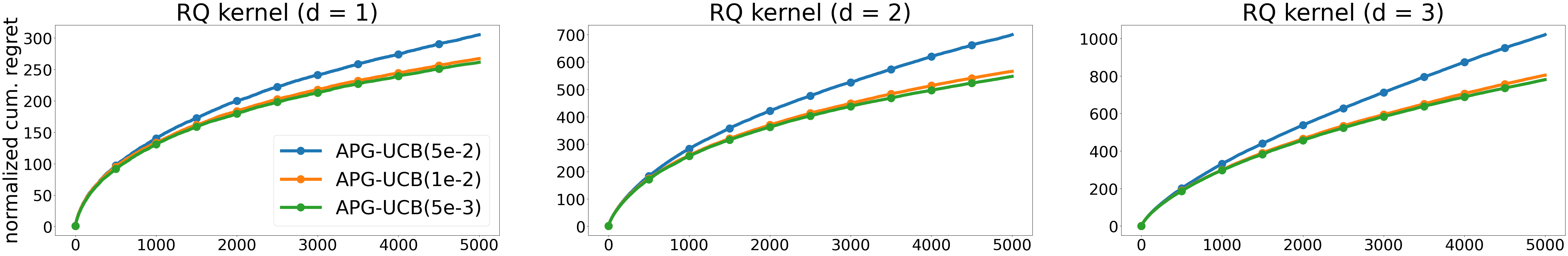
Figure 3: Normalized Cumulative Regret for RQ kernels with $l=0.3\sqrt{d}$.

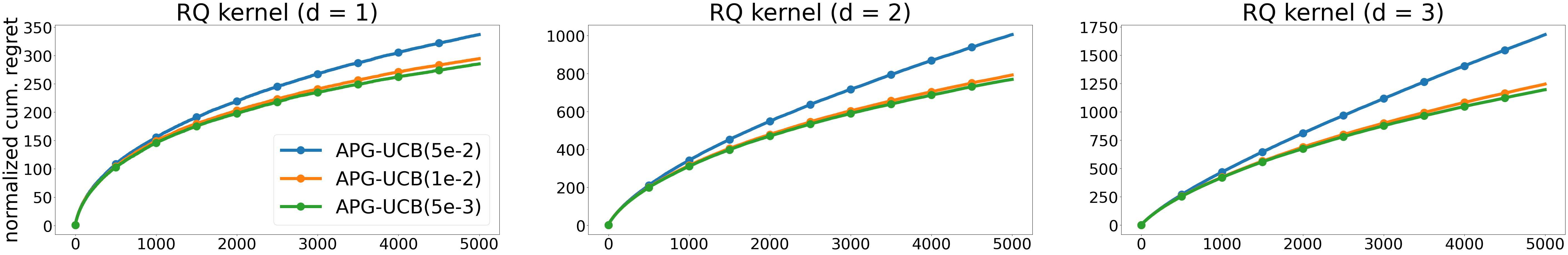
Figure 4: Normalized Cumulative Regret for RQ kernels with $l=0.2\sqrt{d}$.

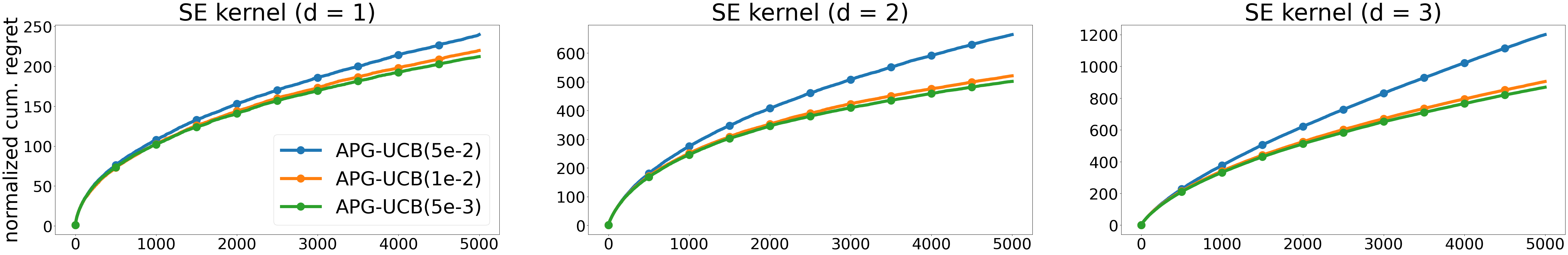
Figure 5: Normalized Cumulative Regret for SE kernels with $l=0.2\sqrt{d}$.

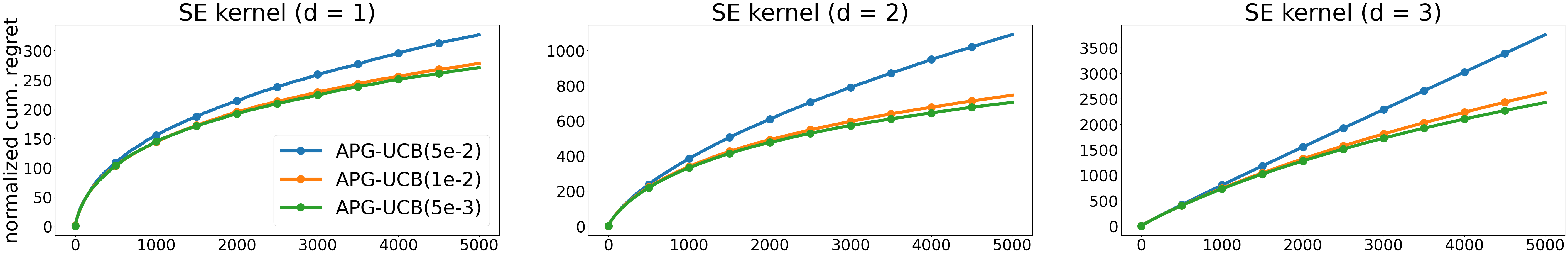
Figure 6: Normalized Cumulative Regret for SE kernels with $l=0.1\sqrt{d}$.

Table 3: Total Running Time for RQ Kernels with $l=0.3\sqrt{d}$.

	APG-UCB(5e-2)	APG-UCB(1e-2)	APG-UCB(5e-3)
d = 1 (RQ)	3.91e-01	4.06e-01	4.23e-01
d = 2 (RQ)	1.36e+00	2.39e+00	2.76e+00
d = 3 (RQ)	1.19e+01	2.40e+01	2.98e+01

Table 4: Total Running Time for SE Kernels with $l=0.2\sqrt{d}$.

	APG-UCB(5e-2)	APG-UCB(1e-2)	APG-UCB(5e-3)
d = 1 (SE)	3.84e-01	4.04e-01	4.02e-01
d = 2 (SE)	1.69e+00	2.59e+00	2.89e+00
d = 3 (SE)	2.13e+01	3.51e+01	4.30e+01

Table 5: Total Running Time for RQ Kernels with $l=0.2\sqrt{d}$.

	APG-UCB(5e-2)	APG-UCB(1e-2)	APG-UCB(5e-3)
d = 1 (RQ)	4.49e-01	4.84e-01	4.96e-01
d = 2 (RQ)	3.84e+00	6.01e+00	7.39e+00
d = 3 (RQ)	4.87e+01	8.76e+01	1.07e+02

Table 6: Total Running Time for SE Kernels with $l=0.1\sqrt{d}$.

	APG-UCB(5e-2)	APG-UCB(1e-2)	APG-UCB(5e-3)
d = 1 (SE)	4.72e-01	4.88e-01	5.08e-01
d = 2 (SE)	9.59e+00	1.40e+01	1.61e+01
d = 3 (SE)	1.77e+02	2.02e+02	2.02e+02

References

• Abbasi-Yadkori et al. (2011) Abbasi-Yadkori, Y., Pál, D., and Szepesvári, C. Improved algorithms for linear stochastic bandits. In Advances in Neural Information Processing Systems, pp. 2312–2320, 2011.
• Agrawal & Goyal (2013) Agrawal, S. and Goyal, N. Thompson sampling for contextual bandits with linear payoffs. In Proceedings of the 30th International Conference on Machine Learning, pp.  127–135, 2013.
• Auer (2002) Auer, P. Using confidence bounds for exploitation-exploration trade-offs. Journal of Machine Learning Research, 3(Nov):397–422, 2002.
• Bubeck & Cesa-Bianchi (2012) Bubeck, S. and Cesa-Bianchi, N. Regret analysis of stochastic and nonstochastic multi-armed bandit problems. Foundations and Trends in Machine Learning, 5(1):1–122, 2012.
• Calandriello et al. (2019) Calandriello, D., Carratino, L., Lazaric, A., Valko, M., and Rosasco, L. Gaussian process optimization with adaptive sketching: Scalable and no regret. In Conference on Learning Theory, pp.  533–557. PMLR, 2019.
• Calandriello et al. (2020) Calandriello, D., Carratino, L., Valko, M., Lazaric, A., and Rosasco, L. Near-linear time gaussian process optimization with adaptive batching and resparsification. In Proceedings of the 37th International Conference on Machine Learning, 2020.
• Chatterji et al. (2019) Chatterji, N., Pacchiano, A., and Bartlett, P. Online learning with kernel losses. In International Conference on Machine Learning, pp. 971–980. PMLR, 2019.
• Chowdhury & Gopalan (2017) Chowdhury, S. R. and Gopalan, A. On kernelized multi-armed bandits. In Proceedings of the 34th International Conference on Machine Learning, pp.  844–853, 2017. supplementary material.
• De Marchi et al. (2005) De Marchi, S., Schaback, R., and Wendland, H. Near-optimal data-independent point locations for radial basis function interpolation. Advances in Computational Mathematics, 23(3):317–330, 2005.
• DeVore et al. (2013) DeVore, R., Petrova, G., and Wojtaszczyk, P. Greedy algorithms for reduced bases in banach spaces. Constructive Approximation, 37(3):455–466, 2013.
• Hoffman et al. (1953) Hoffman, A., Wielandt, H., et al. The variation of the spectrum of a normal matrix. Duke Mathematical Journal, 20(1):37–39, 1953.
• Lattimore & Szepesvári (2020) Lattimore, T. and Szepesvári, C. Bandit Algorithm. Cambridge University Press, 2020.
• Lattimore et al. (2020) Lattimore, T., Szepesvari, C., and Weisz, G. Learning with good feature representations in bandits and in rl with a generative model. In Proceedings of the 37th International Conference on Machine Learning, 2020.
• Madych & Nelson (1992) Madych, W. and Nelson, S. Bounds on multivariate polynomials and exponential error estimates for multiquadric interpolation. Journal of Approximation Theory, 70(1):94–114, 1992.
• Müller (2009) Müller, S. Komplexität und Stabilität von kernbasierten Rekonstruktionsmethoden. PhD thesis, Fakultät für Mathematik und Informatik, Georg-August-Universität Göttingen, 2009.
• Müller & Schaback (2009) Müller, S. and Schaback, R. A newton basis for kernel spaces. Journal of Approximation Theory, 161(2):645–655, 2009.
• Mutny & Krause (2018) Mutny, M. and Krause, A. Efficient high dimensional bayesian optimization with additivity and quadrature fourier features. In Advances in Neural Information Processing Systems, pp. 9005–9016, 2018.
• Pazouki & Schaback (2011) Pazouki, M. and Schaback, R. Bases for kernel-based spaces. Journal of Computational and Applied Mathematics, 236(4):575–588, 2011.
• Pinkus (2012) Pinkus, A. N-widths in Approximation Theory, volume 7. Springer Science & Business Media, 2012.
• Rahimi & Recht (2008) Rahimi, A. and Recht, B. Random features for large-scale kernel machines. In Advances in Neural Information Processing Systems, pp. 1177–1184, 2008.
• Santin & Haasdonk (2017) Santin, G. and Haasdonk, B. Convergence rate of the data-independent $p$-greedy algorithm in kernel-based approximation. Dolomites Research Notes on Approximation, 10(Special_Issue), 2017.
• Scarlett et al. (2017) Scarlett, J., Bogunovic, I., and Cevher, V. Lower bounds on regret for noisy gaussian process bandit optimization. In Conference on Learning Theory, pp.  1723–1742, 2017.
• Schaback (1995) Schaback, R. Error estimates and condition numbers for radial basis function interpolation. Advances in Computational Mathematics, 3(3):251–264, 1995.
• Schaback & Wendland (2000) Schaback, R. and Wendland, H. Adaptive greedy techniques for approximate solution of large rbf systems. Numerical Algorithms, 24(3):239–254, 2000.
• Srinivas et al. (2010) Srinivas, N., Krause, A., Kakade, S., and Seeger, M. Gaussian process optimization in the bandit setting: no regret and experimental design. In Proceedings of the 27th International Conference on Machine Learning, pp.  1015–1022, 2010.
• Valko et al. (2013) Valko, M., Korda, N., Munos, R., Flaounas, I., and Cristianini, N. Finite-time analysis of kernelised contextual bandits. In Proceedings of the 29th Conference on Uncertainty in Artificial Intelligence, 2013.
• Wendland (1997) Wendland, H. Sobolev-type error estimates for interpolation by radial basis functions. Surface fitting and multiresolution methods, pp.  337–344, 1997.
• Wendland (2004) Wendland, H. Scattered data approximation, volume 17. Cambridge University Press, 2004.
• Wu & Schaback (1993) Wu, Z.-m. and Schaback, R. Local error estimates for radial basis function interpolation of scattered data. IMA Journal of Numerical Analysis, 13(1):13–27, 1993.