Reliable Over-the-Air Computation by Amplify-and-Forward Based Relay

Abstract

In typical sensor networks, data collection and processing are separated. A sink collects data from all nodes sequentially, which is very time consuming. Over-the-air computation, as a new diagram of sensor networks, integrates data collection and processing in one slot: all nodes transmit their signals simultaneously in the analog wave and the processing is done in the air. This method, although efficient, requires that signals from all nodes arrive at the sink, aligned in signal magnitude so as to enable an unbiased estimation. For nodes far away from the sink with a low channel gain, misalignment in signal magnitude is unavoidable. To solve this problem, in this paper, we investigate the amplify-and-forward based relay, in which a relay node amplifies signals from many nodes at the same time. We first discuss the general relay model and a simple relay policy. Then, a coherent relay policy is proposed to reduce relay transmission power. Directly minimizing the computation error tends to over-increase node transmission power. Therefore, the two relay policies are further refined with a new metric, and the transmission power is reduced while the computation error is kept low. In addition, the coherent relay policy helps to reduce the relay transmission power by half, to below the limit, which makes it one step ahead towards practical applications.

I Introduction

Many sensor nodes will be deployed to sense the environment so as to support context-aware applications in the future smart society. These sensors will be connected to the Internet via techniques such as NB-IoT and LoRa [1]. In the data collection process, generally, the sink node has to collect data from each node, one by one, which will take a long time when there are millions of nodes in the coverage of a sink node. In addition, many nodes share a common channel, and the increase in the number of nodes will lead to more transmission collisions.

On the other hand, in some tasks, people are only interested in the statistics of sensor data, e.g., the average temperature or moisture in an area, instead of their respective values. For these cases, it is possible to exploit a more efficient method called over-the-air computation (AirComp) [2]. Typically, all nodes simultaneously transmit their signals in the analog wave [3], and the data collection and processing are integrated in one slot. Then, their fusion (sum) is computed by the superposition of electromagnetic waves in the air, at the antenna of the sink. An essential feature of AirComp is the uncoded analog transmission, which seems inferior to digital transmissions. Actually, it is proved that the computation error in AirComp based estimation is exponentially smaller than the digital schemes when using the same amount of resources [4]. Besides the sum operation, AirComp can support any kind of nomographic functions [5, 6, 7], if only proper pre-processing is done at the sensor nodes and post-processing is done at the sink. Recently, deep AirComp is studied, using deep neural networks in the pre-processing and post-processing, which enables more advanced processing of sensor data [8].

To ensure an unbiased data fusion, it is required that signals from all nodes arrive at the sink, aligned in signal magnitude. This is usually achieved by transmission power control at sensor nodes [9, 10]. Specifically, each node uses a transmission power inversely proportional to the channel gain so as to mitigate the difference in channel gains. Obviously, for nodes far away from the sink with a low channel gain, even using the largest transmission power cannot equalize the channel, and the misalignment in signal magnitude unavoidably occurs under the constraint of transmission power, which can be regarded as an outage.

Path diversity by a relay is a conventional and effective method to reducing the outage probability. The decode-and-forward (DF) method applies codes to protect signals. Amplify-and-forward (AF) is simpler, where a relay node simply amplifies the received signal (together with noise). There have been many literature on relay for the unicast communication, either AF [11, 12], DF [13], or their comparison [14]. In addition, network coding-based relay also has been studied for the bidirectional communication [15] and the multiple access channel [16]. In the multiple access channel, compute-and-forward [17] works in a similar way as network coding, where a relay node decodes the linear combination of multiple received messages and forwards it towards the sink. The sink, with efficient equations of messages, can solve each message separately. But these relay methods cannot be directly applied to AirComp. Recently, intelligent reflecting surface (IRS) is suggested for AirComp [18], where a reflection surface, as a passive relay node, is used to shape the phase of each signal. This may be possible for the mmWave band (or higher frequencies) where electromagnetic wave can propagate directionally along desired paths, but it is difficult to apply IRS in a reflection-rich environment for the typical IoT frequency bands (e.g., 920MHz, 2.4GHz).

In this paper, we will investigate how to use relay, more specifically, AF-based relay, to improve the performance of AirComp. To the best of our knowledge, this is the first work on AF-based AirComp. AF is considered because signals in AirComp are transmitted in the analog wave. In the communication, the relay node will amplify signals from many nodes and forward them to the sink, and the whole process should try to ensure the alignment of signal magnitudes at the sink so as to reduce the computation error.

The contribution of this paper is three-fold, as follows:

• We first present the general relay model for AirComp, and investigate a simple relay (SimRelay) policy, in which a node either directly transmits its signal to the sink or via the relay, but not both. Then, we point out the problem: relay transmission power increases with the number of nodes that use the relay node.

• To reduce relay transmission power, we propose a coherent relay (CohRelay) policy, in which a node can divide its power to transmit its signal to both the relay and the sink, and the replicas of its signal are coherently combined together at the sink. We also investigate the impact of the number of nodes using the relay node.

• We discuss the tradeoff between computation error and transmission power. The computation error is composed of signal part and noise part. We find that directly minimizing the computation error may lead to a large increase in node transmission power when the noise part is dominant. Therefore, we further refine the relay policies, avoiding over-reducing the noise part. This has little impact on the computation error, but greatly reduces node transmission power.

Extensive simulation evaluations confirm the effectiveness of the proposed methods. Especially, CohRelay greatly reduces the relay transmission power to below the limit, which makes it one step ahead towards practical applications.

In the rest of this paper, in Sec.II, we review the AirComp model and previous work on improving its performance. Then, in Sec.III, we present the relay model for AirComp, and investigate two relay policies. With some simulation results, we illustrate the problem of over increase in node transmission power. Then, the two relay policies are refined and evaluated in Sec.IV. Finally, in Sec.V, we conclude this paper and point out future work.

II Related Work

Here, we review the AirComp method and previous solutions to channel fading.

II-A Basic over-the-air computation

We first introduce the basic AirComp model [9]. A sensor network is composed of $K$ sensor nodes and 1 sink. The sensing result at the $k_{th}$ node is represented by the signal $x_{k}\in[-v,v]\in\mathbb{C}$, which has zero mean and unit variance ($E(|x_{k}^{2}|)=1$). The sink will compute the sum of sensing data from all nodes. Both the nodes and the sink have a single antenna. To overcome channel fading, the $k_{th}$ node pre-amplifies its signal by a Tx-scaling factor $b_{k}\in\mathbb{C}$. The channel coefficient between sensor $k$ and the sink is $h_{k}\in\mathbb{C}$. The sink further applies a Rx-scaling factor $a\in\mathbb{C}$ to the received signal, as follows

$$s=a\cdot\left(\sum_{k=1}^{K}h_{k}b_{k}x_{k}+n\right),$$ (1)

where $n\in\mathbb{C}$ is the additive white Gaussian noise (AWGN) at the sink with zero mean and power being $\sigma^{2}$. It is assumed that channel coefficient $h_{k}$ is known by both node $k$ and the sink. Then, in a centralized way, the sink can always adjust $b_{k}$ to ensure that $h_{k}b_{k}$ is real and positive. Therefore, in the following, it is assumed that $h_{k}\in\mathbb{R^{+}}$, $b_{k}\in\mathbb{R^{+}}$, and $a\in\mathbb{\mathbb{R^{+}}}$ for the simplicity of analysis.

The computation error is defined as the mean squared error (MSE) between the received signal sum $s$ and the target signal $\sum_{k=1}^{K}x_{k}$, as follows (by using the facts that signals are independent of each other and independent of noise, $E(x_{k})=0$, $E(|x_{k}^{2}|)=1$)

$$MSE \negmedspace=\negmedspace E\left\{|s-\negmedspace\sum_{k=1}^{K}x_{k}|^{2}\right\}=\negmedspace\sum_{k=1}^{K}|ah_{k}b_{k}-1|^{2}+\sigma^{2}|a|^{2}.$$ (2)

With the maximal power constraint, $|b_{k}x_{k}|^{2}$ should be no more than $P^{\prime}$, the maximal power. Let $P_{max}$ denote $P^{\prime}/v^{2}$. Then, we have $b_{k}^{2}\leq P^{\prime}/v^{2}=P_{max}$. By sorting the channel coefficient ($h_{k}$) in the increasing order, the optimal solution (under the power constraint $|b_{k}|^{2}\leq P_{max},k=1,\cdots,K$) depends on a critical number, $i^{\star}$ [9]. A node whose index is below $i^{\star}$ uses the maximal power $P_{max}$, and otherwise uses a power inversely proportional to the channel gain. Then, the computation MSE is computed as follows:

$$MSE =\sum_{k=1}^{i^{\star}}|ah_{k}\sqrt{P_{max}}-1|^{2}+\sigma^{2}|a|^{2}.$$ (3)

This computation MSE may be caused by channel fading or noise. The former decides the error in the signal magnitude of $i^{\star}$ weak signals and the latter decides the term $\sigma^{2}|a|^{2}$.

II-B Previous improvement on AirComp

When some nodes are far away from the sink, the magnitudes of their signals cannot be aligned with that of other signals from nearer nodes. Some efforts have been devoted to solving this problem. The work in [9] studies the power control policy, aiming to minimize the computation error by jointly optimizing the transmission power and a receive scaling factor at the sink node. Generally, the principle of channel inversion is adopted. Specifically, with the common signal magnitude being $\alpha$ ($\alpha=1/a$), the transmission power of node $k$ is computed as $b_{k}=min\{\alpha/h_{k},\sqrt{P_{max}}\}$, being the former if $\alpha/h_{k}$ is below the power constraint, and otherwise, using the maximal power. In [10], the authors further consider the time-varying channel by regularized channel inversion, aiming at a better tradeoff between the signal-magnitude alignment and noise suppression. Antenna array was also investigated in [19, 20] to support vector-valued AirComp.

AirComp is an efficient solution in federated learning, where the model update is to be transmitted from each node to the common sink, aggregated there, and then sent back to each node for future data processing. Specific consideration on AirComp is also studied. Because information from some of the nodes is sufficient, node selection based on the channel gain is suggested in [21], although this does not apply to general AirComp where signals from all nodes are needed. Sery et al. further suggests precoding and scaling operations to gradually mitigate the effect of the noisy channel so as to facilitate the convergence of the learning process [22].

III AirComp with AF-based relay

A wireless signal attenuates as the propagation distance increases. With a single antenna, the effect of transmission power control in dealing with path loss and channel fading is limited. Therefore, we try to exploit relay, which has been proven to be effective in conventional unicast communications.

III-A System framework

The network consists of $K$ sensor nodes, a relay $r$ and a sink $d$. Sink $d$ will compute the sum of sensing data from all nodes, via the help of relay $r$. All nodes, relay $r$ and sink $d$ use a single antenna. Each node has a constraint of the maximal transmission power. But we assume that the relay has no constraint of transmission power, and investigate how much power is required for relaying signals. Nodes near to the sink can directly communicate with the sink, while nodes farther away can rely on the relay to help. Then, all nodes are divided into two groups. A node $k$ is either a neighbor of $r$ ($k\in N_{r}$) and will use relay $r$, or a non-neighbor of $r$ ($k\in N_{d}$) and will directly transmit its signal to sink $d$. Fig.1 shows an analogy to a conventional relay network. The difference is that there are more than one node in $N_{r}$ and $N_{d}$.

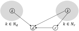
Figure 1: Relay for AirComp, an analogy to a conventional relay network.

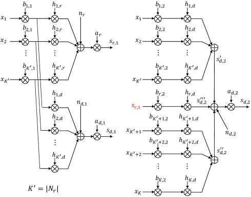
Figure 2: Detailed relay model for AirComp. $K$ sensor nodes each have a signal to send to the common sink. Nodes in $N_{r}$ transmit their signals to the sink via the relay, while nodes in $N_{d}$ directly transmit their signals to the sink.

We assume that (i) the sensor network is fixed without node mobility, and channel coefficients ($h_{k,r}\in\mathbb{C}$ and $h_{k,d}\in\mathbb{C}$, representing channel coefficients from node $k$ to relay $r$ and sink $d$, respectively) are constant within a period of time, (ii) each node (and relay $r$) knows channel coefficients of its links to sink $d$ and relay $r$, and (iii) channel coefficients of all links are known to sink $d$, which decides the node grouping policy (decides which nodes to use the relay) and other parameters.

Similar to the conventional AF method, the whole transmission is divided into two slots. But the transmission powers (Tx-scaling factor $b_{k,1}\in\mathbb{C}$ and $b_{k,2}\in\mathbb{C}$ in two time slots) are adjusted per node per slot. The detailed process is shown in Fig.2.

In the first slot, a neighbor node ($k\in N_{r}$) of relay $r$ transmits its signal using a Tx-scaling factor $b_{k,1}$. The signals received at relay $r$ and sink $d$ are

$$s_{r,1}=a_{r,1}\cdot\left(\sum_{k\in N_{r}}h_{k,r}b_{k,1}x_{k}+n_{r,1}\right),$$ (4)

$$s_{d,1}=a_{d,1}\cdot\left(\sum_{k\in N_{r}}h_{k,d}b_{k,1}x_{k}+n_{d,1}\right),$$ (5)

where $a_{r,1}\in\mathbb{C}$ and $a_{d,1}\in\mathbb{C}$ are Rx-scaling factors, and $n_{r,1}$ and $n_{d,1}$ are AWGN noises with zero mean and variance being $\sigma^{2}$.

In the second slot, all nodes transmit their signals to sink $d$, and node $k$ uses a Tx-scaling factor $b_{k,2}$. Meanwhile relay $r$ also forwards its received signal, using a Tx-scaling factor $b_{r,2}$. Signals arriving at sink $d$ are composed of 3 parts, as follows:

$$s^{\prime}_{d,2}=\sum_{k\in N_{r}}h_{k,d}b_{k,2}x_{k},$$ (6)

$$s^{\prime\prime}_{d,2}=\sum_{k\in N_{d}}h_{k,d}b_{k,2}x_{k},$$ (7)

$$s^{\prime\prime\prime}_{d,2}=h_{r,d}b_{r,2}s_{r,1},$$ (8)

where $s^{\prime}_{d,2}$ is the signal from $k\in N_{r}$, $s^{\prime\prime}_{d,2}$ is the signal from $k\in N_{d}$, and $s^{\prime\prime\prime}_{d,2}$ is the relayed signal. Then, the overall signal at the second slot is

$$s_{d,2}=a_{d,2}\cdot\left(s^{\prime}_{d,2}+s^{\prime\prime}_{d,2}+s^{\prime\prime\prime}_{d,2}+n_{d,2}\right),$$ (9)

where $a_{d,2}\in\mathbb{C}$ is a Rx-scaling factor, and $n_{d,2}$ is AWGN noise with zero mean and variance being $\sigma^{2}$.

Sink $d$ adds the signals received in the two slots. For a signal from a neighbor ($k\in N_{r}$) of relay $r$, its overall coefficient at the sink is

$$\beta_{k} =a_{d,1}h_{k,d}b_{k,1}+a_{d,2}h_{k,d}b_{k,2}$$

$$+a_{d,2}h_{r,d}b_{r,2}\cdot a_{r,1}h_{k,r}b_{k,1},k\in N_{r}.$$ (10)

Its first term corresponds to the signal directly received in the first slot, its second term corresponds to the signal directly received in the second slot, and its third term corresponds to the relayed signal.

For a signal from a node not a neighbor ( $k\in N_{d}$) of relay $r$, its coefficient at sink $d$ is

$$\beta_{k}=a_{d,2}h_{k,d}b_{k,2},k\in N_{d}.$$ (11)

The overall noise is

$$n_{a}=a_{d,1}n_{d,1}+a_{d,2}n_{d,2}+a_{d,2}h_{r,d}b_{r,2}\cdot a_{r,1}n_{r,1}.$$ (12)

All the parameters are to be solved by minimizing the following computation MSE (under the power constraint $|b_{k,1}|^{2}\leq P_{max},|b_{k,2}|^{2}\leq P_{max},k=1,\cdots,K$).

$$MSE \negmedspace=\negmedspace E\left\{|\sum_{k=1}^{K}\beta_{k}x_{k}\negmedspace+\negmedspace n_{a}\negmedspace-\negmedspace\sum_{k=1}^{K}x_{k}|^{2}\right\}\negmedspace=\negmedspace\sum_{k=1}^{K}|\beta_{k}-1|^{2}$$

$$+\sigma^{2}(|a_{d,1}|^{2}+|a_{d,2}|^{2}+|a_{d,2}h_{r,d}b_{r,2}a_{r,1}|^{2}).$$ (13)

It is difficult to directly solve this problem. In the following, we discuss its solution under several relay policies.

III-B Nodes grouping and relay transmission power

Different from a conventional relay method, relay $r$ has to amplify $|N_{r}|$ signals, and the overall signal to be relayed is

$$\sum_{k\in N_{r}}a_{r,1}h_{k,r}b_{k,1}x_{k}.$$ (14)

To ensure that all signals are aligned in magnitude at sink $d$, the magnitude of the relayed signals ($a_{d,2}h_{r,d}b_{r,2}\cdot a_{r,1}h_{k,r}b_{k,1}$, $k\in N_{r}$) should approach that of directly received signals ($a_{d,2}h_{k,d}b_{k,2}$, $k\in N_{d}$). Here, relay $r$ will use a Tx-scaling factor $b_{r,2}$ which depends on node transmission power ($b_{k,1}$), channel gains ($h_{r,d}$, $h_{k,r}$), and alignment with other nodes ($a_{d,2}$, $a_{r,1}$). The transmission power required at the relay node is

$$|b_{r,2}|^{2}\cdot\sum_{k\in N_{r}}|a_{r,1}h_{k,r}b_{k,1}|^{2}.$$ (15)

Obviously, the relay transmission power linearly increases with the number of nodes using the relay, which is a big problem. Therefore, it is impractical to use relay for all nodes.

To solve this problem, we propose that nodes far away from sink $d$ while near to relay $r$ should use the relay. Therefore, nodes are sorted in the ascending order of $|h_{k,d}|^{2}-|h_{k,r}|^{2}$, the difference of channel gain to sink $d$ and relay $r$. The top nodes will use relay $r$, and the percentage of nodes using relay $r$ is a parameter.

III-C Simple Relay Policy

We first consider a simple relay (SimRelay) policy. $s_{d,1}$ is neglected ($a_{d,1}=0$) and $s^{\prime}_{d,2}$ is not transmitted ($b_{k,2}=0,k\in N_{r}$). In other words, in the first slot, signals from $k\in N_{r}$ are sent to relay $r$, and in the second slot, signals from $k\in N_{d}$ are directly sent to sink $d$ and signals from $k\in N_{r}$ are forwarded to sink $d$ by relay $r$. This is the most simple relay method: the direct link is neglected once the relay is used.

With $a_{d,1}=0$, $b_{k,2}=0$ ($k\in N_{r}$), and $a_{d,2}h_{r,d}b_{r,2}=c$, the computation MSE in Eq.(13) can be rewritten as

$$MSE =\sum_{k\in N_{r}}|(ca_{r,1})h_{k,r}b_{k,1}-1|^{2}+\sigma^{2}|ca_{r,1}|^{2}$$

$$+\sum_{k\in N_{d}}|a_{d,2}h_{k,d}b_{k,2}-1|^{2}+\sigma^{2}|a_{d,2}|^{2}.$$ (16)

Because $c$ can be merged into $a_{r,1}$, we denote their product as $a^{\prime}_{r,1}=ca_{r,1}$, and the computation MSE can be computed as the sum of

$$MSE_{r} =\sum_{k\in N_{r}}|a^{\prime}_{r,1}h_{k,r}b_{k,1}-1|^{2}+\sigma^{2}|a^{\prime}_{r,1}|^{2},$$

$$MSE_{d} =\sum_{k\in N_{d}}|a_{d,2}h_{k,d}b_{k,2}-1|^{2}+\sigma^{2}|a_{d,2}|^{2}.$$ (17)

Because $MSE_{r}$ and $MSE_{d}$ depend on different nodes and different parameters, the relay problem is equivalent to two AirComp problems, one from $k\in N_{r}$ to relay $r$ in the first slot, and the other from $k\in N_{d}$ to sink $d$ in the second slot. Each can be solved by using the power control algorithm suggested in [9]. Because $b_{k,1}$ and $b_{k,2}$ can be adjusted to ensure $h_{k,r}b_{k,1}$ and $h_{k,d}b_{k,2}$ are positive real numbers, in the analysis, $h_{k,r}\in\mathbb{R^{+}}$, $h_{k,d}\in\mathbb{R^{+}}$, $b_{k,1}\in\mathbb{R^{+}}$, $b_{k,2}\in\mathbb{R^{+}}$, $a^{\prime}_{r,1}\in\mathbb{R^{+}}$, $a_{d,2}\in\mathbb{R^{+}}$ are assumed for the simplicity of analysis.

In SimRelay, relay $r$ has to amplify the whole signals from $|N_{r}|$ nodes, which requires much transmission power.

III-D Coherent Relay Policy

To reduce relay transmission power, we consider a coherent relay (CohRelay) policy. A node using relay divides its power into two parts, and transmits its signal twice. Sink $d$ receives two coherent copies of the same signal and adds them together.

In this case, $s_{d,1}$ is neglected ($a_{d,1}=0$) but $s^{\prime}_{d,2}$ ($k\in N_{r}$) is transmitted. Compared with SimRelay, the difference is that in the second slot, nodes $k\in N_{r}$ transmit their signals again. With $a_{d,1}=0$, $a_{d,2}h_{r,d}b_{r,2}=c$, and $a^{\prime}_{r,1}=ca_{r,1}$, the computation MSE in Eq.(13) can be rewritten as

$$MSE =\sum_{k\in N_{r}}|a_{d,2}h_{k,d}b_{k,2}+a^{\prime}_{r,1}h_{k,r}b_{k,1}-1|^{2}+\sigma^{2}|a^{\prime}_{r,1}|^{2}$$

$$+\sum_{k\in N_{d}}|a_{d,2}h_{k,d}b_{k,2}-1|^{2}+\sigma^{2}|a_{d,2}|^{2}.$$ (18)

Because $a_{d,2}$ also appears in the first sum, this cannot be simply divided into two AirComp problems like SimRelay. But $h_{k,r}\in\mathbb{R^{+}}$, $h_{k,d}\in\mathbb{R^{+}}$, $b_{k,1}\in\mathbb{R^{+}}$, $b_{k,2}\in\mathbb{R^{+}}$, $a^{\prime}_{r,1}\in\mathbb{R^{+}}$, $a_{d,2}\in\mathbb{R^{+}}$ can be assumed in the analysis. Then, $a_{d,2}h_{k,d}b_{k,2}$ in the first sum is a positive real number. Without this term, like SimRelay, an initial estimation of $a^{\prime}_{r,1}$ and $a_{d,2}$ can be computed, by minimizing $MSE_{r}$ and $MSE_{d}$ in Eq.(17), respectively.

Next consider the presence of $a_{d,2}h_{k,d}b_{k,2}$ in the first sum of Eq.(18). Assume originally some $a^{\prime}_{r,1}$ and $b_{k,1}$ make $a^{\prime}_{r,1}h_{k,r}b_{k,1}$ equal to 1.0 (or approach 1 under the maximal power constraint). If $b_{k,1}$ is fixed, the presence of $a_{d,2}h_{k,d}b_{k,2}$ (a positive number) makes it possible to use a smaller $a^{\prime}_{r,1}$ to make $a_{d,2}h_{k,d}b_{k,2}+a^{\prime}_{r,1}h_{k,r}b_{k,1}$ reach 1.0. Meanwhile, the term $\sigma^{2}|a^{\prime}_{r,1}|^{2}$ also decreases. In other words, it is possible to decrease $a^{\prime}_{r,1}$ in a certain range to reduce the first sum in Eq.(18). Therefore, a heuristic algorithm is to use the initial estimation of $a^{\prime}_{r,1}$ as a seed, and then gradually decrease it to find the minimum while fixing $a_{d,2}$ (ensuring the minimum of the second sum in Eq.(18)).

Actually, $b_{k,1}$ and $b_{k,2}$ depend on the setting of $a^{\prime}_{r,1}$ and $a_{d,2}$. In addition, to ensure a fair comparison with SimRelay, it is assumed that the overall power, $|b_{k,1}|^{2}+|b_{k,2}|^{2}=P$, should be no more than $P_{max}$. Then, the power allocation for $b_{k,1}$ and $b_{k,2}$ ($k\in N_{r}$) is to maximize the term $a_{d,2}h_{k,d}b_{k,2}+a^{\prime}_{r,1}h_{k,r}b_{k,1}$, under the power constraint. According to the Cauchy–Schwarz inequality [23]

$$\left((a^{\prime}_{r,1}h_{k,r})b_{k,1}+(a_{d,2}h_{k,d})b_{k,2}\right)^{2}$$

$$\leq\left((a^{\prime}_{r,1}h_{k,r})^{2}+(a_{d,2}h_{k,d})^{2}\right)\left(b_{k,1}^{2}+b_{k,2}^{2}\right),$$ (19)

and the equality holds if and only if

$$\frac{b_{k,1}}{a^{\prime}_{r,1}h_{k,r}}=\frac{b_{k,2}}{a_{d,2}h_{k,d}}=\rho_{k}.$$ (20)

Then, with $|b_{k,1}|^{2}+|b_{k,2}|^{2}=P\leq P_{max}$, $\rho_{k}$ can be computed as

$$\rho_{k}(P)=\frac{\sqrt{P}}{\sqrt{\left(a^{\prime}_{r,1}h_{k,r}\right)^{2}+\left(a_{d,2}h_{k,d}\right)^{2}}}.$$ (21)

On this basis, $b_{k,1}$ and $b_{k,2}$ are computed from Eq.(20), and the value of $a_{d,2}h_{k,d}b_{k,2}+a^{\prime}_{r,1}h_{k,r}b_{k,1}$ is computed as

$$\gamma_{k}(P) =\rho_{k}(P)\cdot\left((a^{\prime}_{r,1}h_{k,r})^{2}+(a_{d,2}h_{k,d})^{2}\right).$$ (22)

If $\gamma_{k}(P_{max})$ is greater than 1.0, setting $\gamma_{k}(P)=1$ can find $\rho_{k}(P)$ and the powers ($b_{k,1}$ and $b_{k,2}$) that lead to 0 error in the signal magnitude.

The whole process of finding optimal parameters and the corresponding computation MSE is described in Algorithm 1.

1:procedure FindParamForCohRelay($h_{k,r}$, $h_{k,d}$)

2:     Initialize $a_{d,2}$, by minimizing $MSE_{d}$ in Eq.(17)

3:     Initialize $a^{\prime}_{r,1}$, by minimizing $MSE_{r}$ in Eq.(17)

4:     $MSE_{rd}$ = OneIter($h_{k,r}$, $h_{k,d}$, $a^{\prime}_{r,1}$, $a_{d,2}$)

5:     while $True$ do $\triangleright$ Iteration

6:         $MSE^{\prime}_{rd}$ = OneIter($h_{k,r}$, $h_{k,d}$, $a^{\prime}_{r,1}\negmedspace-\negmedspace\delta$, $a_{d,2}$)

7:         if $MSE^{\prime}_{rd}<MSE_{rd}$ then

8:              $a^{\prime}_{r,1}\leftarrow a^{\prime}_{r,1}-\delta$ $\triangleright$ Update $a^{\prime}_{r,1}$

9:              $MSE_{rd}\leftarrow MSE^{\prime}_{rd}$

10:         else

11:              break

12:         end if

13:     end while

14:     return $MSE_{d}(a_{d,2})+MSE_{rd}$

15:end procedure

16:procedure OneIter($h_{k,r}$, $h_{k,d}$, $a^{\prime}_{r,1}$, $a_{d,2}$)

17:     for $k\in N_{r}$ do$\triangleright$ Iteration on $N_{r}$

18:         

19:         $\rho_{k}(P_{max})=\sqrt{P_{max}}/\sqrt{\left(a^{\prime}_{r,1}h_{k,r}\right)^{2}+\left(a_{d,2}h_{k,d}\right)^{2}}$

20:         $\gamma_{k}(P_{max})\negmedspace=\negmedspace\rho_{k}(P_{max})\cdot\left(\negmedspace\left(a^{\prime}_{r,1}h_{k,r}\right)^{2}\negmedspace+\negmedspace\left(a_{d,2}h_{k,d}\right)^{2}\negmedspace\right)$

21:         if $\gamma_{k}(P_{max})\geq 1$  then

22:              $\rho_{k}(P)=1/\left(\left(a^{\prime}_{r,1}h_{k,r}\right)^{2}+\left(a_{d,2}h_{k,d}\right)^{2}\right)$

23:              $b_{k,1}=\rho_{k}(P)\cdot a^{\prime}_{r,1}h_{k,r}$

24:              $b_{k,2}=\rho_{k}(P)\cdot a{}_{d,2}h_{k,d}$

25:              $e_{k}=0$

26:         else

27:              $b_{k,1}=\rho_{k}(P_{max})\cdot a^{\prime}_{r,1}h_{k,r}$

28:              $b_{k,2}=\rho_{k}(P_{max})\cdot a{}_{d,2}h_{k,d}$

29:              $e_{k}=1-\gamma_{k}(P_{max})$

30:         end if

31:     end for

32:     $MSE_{rd}=\sum_{k\in N_{r}}e_{k}^{2}+\sigma^{2}|a^{\prime}_{r,1}|^{2}$

33:     return $MSE_{rd}$

34:end procedure

Algorithm 1 Find optimal parameters and compute MSE.

In CohRelay, $a_{d,2}h_{k,d}b_{k,2}+a^{\prime}_{r,1}h_{k,r}b_{k,1}\approx 1$ so $a^{\prime}_{r,1}h_{k,r}b_{k,1}$ is less than 1. This helps to reduce the relay transmission power in Eq.15.

III-E Simulation Evaluation

Here, we evaluate the relay methods discussed in the previous sections, by comparing them with the AirComp method [9] that only exploits the direct link.

Figure 3 shows the simulation scenario. 50 sensor nodes are randomly and uniformly distributed in a rectangle area. The path loss model uses a hybrid free-space/two-ray model and each link experiences independent slow Rayleigh fading (channel gains are the same in two slots). We assume that the link $rd$ does not experience fading by properly selecting a relay node not in fading (the relay selection itself is left as future work). The noise level is -90dBm. It is assumed that both sink $d$ and relay $r$ amplifies the signal with a gain of 90dB. The simulation is run 10,000 times using the Matlab software. Main parameters are listed in Table I.

TABLE I: Main parameters for evaluation.

Term	Value
Area	400m x 200m
# nodes	50
Frequency	2.4GHz
Channel	Free-space/two-ray, Rayleigh fading
Power	$P_{max}=10$, $\sigma^{2}=1$

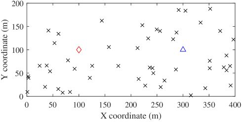
Figure 3: An illustration of simulation scenario with 50 nodes ($\times$) randomly distributed in a 400m x 200m area, 1 sink ($\diamondsuit$, (100, 100)) and 1 relay ($\triangle$, (300, 100)). Node deployment changes per evaluation.

Figure 4 shows the cumulative distribution functions (CDF) of computation MSE, average node transmission power and relay transmission power in different methods. Obviously, AirComp using only direct links has much larger computation MSE than relay methods. SimRelay and CohRelay have almost the same performance in reducing the computation MSE, but CohRelay has much smaller relay transmission power than SimRelay. Surprisingly, both CohRelay and SimRelay require more node transmission power than AirComp.

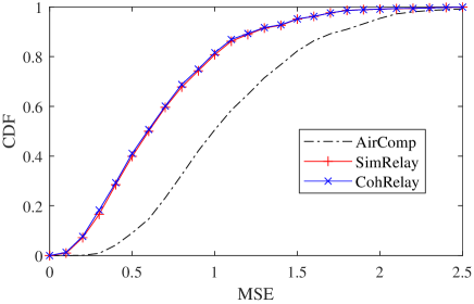
(a) CDF of computation MSE

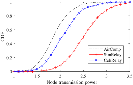
(b) CDF of average node transmission power

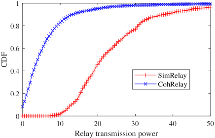
(c) CDF of relay transmission power

Figure 4: Cumulative distribution function of computation MSE, average node transmission power, and relay transmission power in different methods (30% nodes use relay).

IV Refinement of the Relay Methods

In the following, we analyze the computation MSE in CohRelay and refine the parameters. A similar analysis applies to SimRelay.

In Eq.(18), the computation MSE is composed of the signal part and the noise part. When reducing the computation MSE, at first mainly MSE of the signal part is reduced to align signal magnitudes. When MSE of the signal part gets small and the noise becomes dominant, MSE of the noise part is also reduced, which leads to smaller $a^{\prime}_{r,1}$ and $a_{d,2}$, and increased power ($b_{k,1}$ and $b_{k,2}$).

In the original AirComp, MSE of the noise part is $a^{2}\sigma^{2}$. To avoid over-reducing MSE of the noise part in CohRelay, we restrict $((a^{\prime}_{r,1})^{2}+d_{d,2}^{2})\sigma^{2}$ to be no less than $\gamma\cdot a^{2}\sigma^{2}$, where $\gamma$ is a parameter (later it is set to 1.0 based on simulation results). In addition, MSE of the signal part is not a continuous function. Actually it is a constant when $a^{\prime}_{r,1}$ and $a_{d,2}$ change within a range, because the variation is absorbed by adjusting $b_{k,1}$ and $b_{k,2}$, which change continuously. Then, a small decrease in the computation MSE may lead to a large increase in transmission power. To capture this feature, we consider a new metric, involving both the computation MSE and node transmission power (TxP), as follows, where $\theta$ is a parameter.

$$\underset{a^{\prime}_{r,1},a_{d,2},(a^{\prime}_{r,1})^{2}+a_{d,2}^{2}\geq\gamma\cdot a^{2}}{argmin}\theta\cdot MSE+(1-\theta)\cdot TxP,$$ (23)

$$TxP=\frac{1}{K}\sum_{k\in N_{r}\cup N_{d}}b_{k,1}^{2}+b_{k,2}^{2}.$$

With each candidate $a_{d,2}$ in a certain range, $a^{\prime}_{r,1}$ is computed from $\sqrt{\gamma\cdot a^{2}-a_{d,2}^{2}}$. With $a^{\prime}_{r,1}$ and $a_{d,2}$, transmission power ($b_{k,1}$, $b_{k,2}$) for node $k\in N_{r}$ is computed using the function OneIter in Algorithm 1. For node $k\in N_{d}$, $b_{k,2}$ is computed from $a_{d,2}$. Then, the computation MSE and average TxP are computed. Because their values are of the same order of magnitude, $\theta$ is set to 0.5.

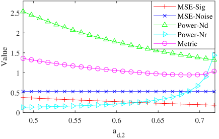
Figure 5: Variation of different metrics with $a_{d,2}$ ($\gamma=1.0$).

With this new metric, we evaluate MSEs of the signal part and the noise part, average transmission power of nodes in $N_{r}$ and $N_{d}$, and the metric in Eq.(23). The results are shown in Fig.5. MSE of noise part is kept constant, as expected. With the increase of $a_{d,2}$, transmission power of nodes in $N_{d}$ decreases. Meanwhile $a^{\prime}_{r,1}$ decreases, which leads to a quick increase in transmission power of nodes in $N_{r}$ when $a_{d,2}$ is large ($a^{\prime}_{r,1}$ is small). The overall MSE of the signal part decreases. Then, the metric, as a weighted sum of the overall MSE and average power, reaches a minimum somewhere, which prefers to use a smaller transmission power when the computation MSE has no significant change.

Next, we evaluate the computation MSE, node transmission power, and relay transmission power, by changing the parameter $\gamma$. Hereafter, the refined relay methods are renamed as SimRelay+ and CohRelay+, respectively. The results are shown in Fig.6. At $\gamma=200\%$, it is equivalent that noise at the relay and the sink are directly added together. When $\gamma$ decreases from 200% to 100%, MSE of the noise part is also reduced, so the overall MSE gradually decreases, meanwhile node and relay transmission power increases, although slowly. When $\gamma$ further decreases, the decrease in the computation MSE becomes smaller while the increase in node transmission power becomes larger. Therefore, in the following evaluation, $\gamma$ is set to 100%.

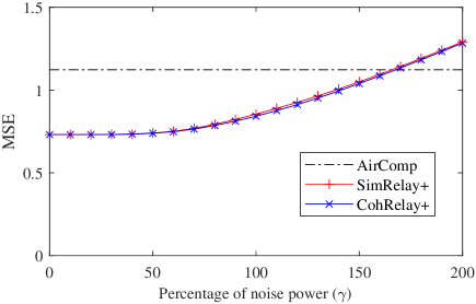
(a) Computation MSE

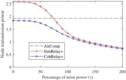
(b) Average node transmission power

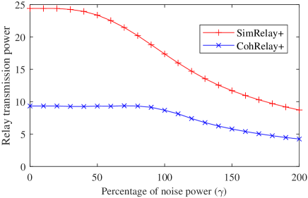
(c) Relay transmission power

Figure 6: Computation MSE, average node transmission power, and relay transmission power in different methods. (30% nodes use relay).

With $\gamma=100\%$, we re-evaluate the computation MSE, node and relay transmission power. The results are shown in Fig.7. The reduction of the computation MSE in CohRelay+ compared with AirComp, decreases from 35.6% (Fig.4(a)) to 25.0%. But the reduction of average node transmission power in CohRelay+ is greatly improved from -10.0% (Fig.4(b)) to 37.0%.

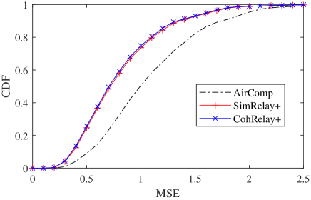
(a) CDF of computation MSE

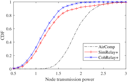
(b) CDF of average node transmission power

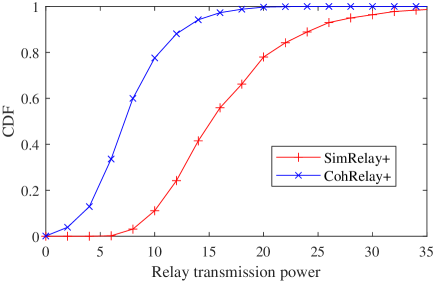
(c) CDF of relay transmission power

Figure 7: Cumulative distribution function of computation MSE, average node transmission power, and relay transmission power in different methods. (30% nodes use relay. $\gamma=100\%$).

We further investigate the impact of the percentage of nodes using relay. As shown in Fig.8, when only a small percentage of nodes use the relay, the reduction of the computation MSE is limited. Node transmission power is relatively large but the relay transmission power is small. When more nodes use relay, the computation MSE is further reduced, so is node transmission power, but relay transmission power increases. In all cases, CohRelay+ achieves almost the same (or a little smaller) computation MSE as SimRelay+, but reduces node transmission power, and especially reduces the relay transmission power by half or more when the percentage of nodes using relay is less than 30%. In this range, the relay transmission power in CohRelay+ is less than $P_{max}$, which makes it practical to use a relay node.

(a) Computation MSE

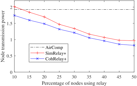
(b) Average node transmission power

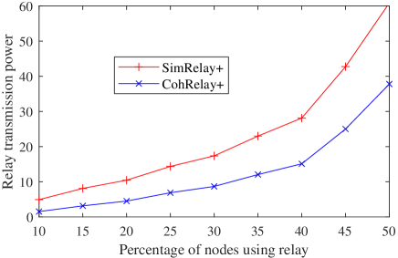
(c) Relay transmission power

Figure 8: Computation MSE, average node transmission power, and relay transmission power with respect to different percentages of nodes using the relay ($\gamma=100\%$).

In the above evaluation, node transmission power and relay transmission power are separately evaluated, and a relay is not used in AirComp. For a fair comparison, we further investigate the overall transmission power of all nodes and the relay. The result is shown in Fig.9. With the increase of the percentage of nodes using relay, the overall transmission power in SimRelay+ and CohRelay+ decreases at first, because using relay helps to reduce node transmission power, and then increases because of the large transmission power at the relay. When the percentage of nodes using relay is no more than 50%, CohRelay+ consumes less overall transmission power than AirComp.

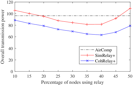
Figure 9: Overall transmission power of all nodes and the relay, under different percentages of nodes using the relay ($\gamma=100\%$).

In sum, using a relay, SimRelay+ and CohRelay+ reduce node transmission power and have a similar performance in reducing the computation MSE, compared with AirComp. This is achieved at the cost of one more slot, and potentially more transmission power. As for the overall transmission power, SimRelay+ may consume more power, but CohRelay+ always consume less power than AirComp in the typical range (the percentage of nodes using relay is less than 50%). Compared with SimRelay+, CohRelay+ reduces the relay transmission power by half or even more, to below the limit when the percentage of nodes using relay is no more than 30%, which facilitates the practical application of AirComp.

V Conclusion

AirComp greatly improves the efficiency of data collection and processing in sensor networks. But its performance is degraded when signals of nodes far away from the sink cannot arrive at the sink, aligned in signal magnitude. To address this problem, this paper investigates the amplify and forward based relay method, and discusses practical issues such as the large relay transmission power and the over-increase of node transmission power. As for the two relay polices, SimRelay+, being simple, effectively reduces the computation MSE and node transmission power. With coherent combination of direct signals and relayed signals, CohRelay+ further reduces the node transmission power and relay transmission power. Although it is impractical for all nodes to use the relay, CohRelay+ helps to reduce the computation MSE meanwhile keeping the relay transmission power below the limit by adjusting the percentage of nodes using relay. In the future, we will further study the relay selection problem.

References

- [1] R. S. Sinha, Y. Wei, and S.-H. Hwang, “A survey on LPWA technology: LoRa and NB-IoT,” ICT Express, vol. 3, no. 1, pp. 14 – 21, 2017. [Online]. Available: http://www.sciencedirect.com/science/article/pii/S2405959517300061
- [2] B. Nazer and M. Gastpar, “Computation over multiple-access channels,” IEEE Transactions on Information Theory, vol. 53, no. 10, pp. 3498–3516, 2007.
- [3] J. Xiao, S. Cui, Z. Luo, and A. J. Goldsmith, “Linear coherent decentralized estimation,” IEEE Transactions on Signal Processing, vol. 56, no. 2, pp. 757–770, 2008.
- [4] C.-Z. Lee, L. P. Barnes, and A. Ozgur, “Over-the-air statistical estimation,” in IEEE Globecom Proceedings, 2020.
- [5] R. C. Buck, “Approximate complexity and functional representation,” J. Math. Anal. Appl., vol. 70, pp. 280–298, 1979.
- [6] M. Goldenbaum, H. Boche, and S. Staczak, “Nomographic functions: Efficient computation in clustered gaussian sensor networks,” IEEE Transactions on Wireless Communications, vol. 14, no. 4, pp. 2093–2105, 2015.
- [7] O. Abari, H. Rahul, and D. Katabi, “Over-the-air function computation in sensor networks,” CoRR, vol. abs/1612.02307, 2016. [Online]. Available: http://arxiv.org/abs/1612.02307
- [8] H. Ye, G. Y. Li, and B.-H. F. Juang, “Deep over-the-air computation,” in IEEE Globecom Proceedings, 2020.
- [9] W. Liu, X. Zang, Y. Li, and B. Vucetic, “Over-the-air computation systems: Optimization, analysis and scaling laws,” IEEE Transactions on Wireless Communications, vol. 19, no. 8, pp. 5488–5502, 2020.
- [10] X. Cao, G. Zhu, J. Xu, and K. Huang, “Optimized power control for over-the-air computation in fading channels,” IEEE Transactions on Wireless Communications, vol. 19, no. 11, pp. 7498–7513, 2020.
- [11] Y. Zhao, R. Adve, and T. J. Lim, “Improving amplify-and-forward relay networks: Optimal power allocation versus selection,” in 2006 IEEE International Symposium on Information Theory, 2006, pp. 1234–1238.
- [12] S. Yang and J. Belfiore, “Towards the optimal amplify-and-forward cooperative diversity scheme,” IEEE Transactions on Information Theory, vol. 53, no. 9, pp. 3114–3126, 2007.
- [13] T. Wang, A. Cano, G. B. Giannakis, and J. N. Laneman, “High-performance cooperative demodulation with decode-and-forward relays,” IEEE Transactions on Communications, vol. 55, no. 7, pp. 1427–1438, 2007.
- [14] M. R. Souryal and B. R. Vojcic, “Performance of amplify-and-forward and decode-and-forward relaying in rayleigh fading with turbo codes,” in 2006 IEEE International Conference on Acoustics Speech and Signal Processing Proceedings, vol. 4, 2006, pp. IV–IV.
- [15] P. Popovski and H. Yomo, “Wireless network coding by amplify-and-forward for bi-directional traffic flows,” IEEE Communications Letters, vol. 11, no. 1, pp. 16–18, 2007.
- [16] S. Tang, J. Cheng, C. Sun, R. Miura, and S. Obana, “Joint channel and network decoding for XOR-based relay in multi-access channel,” IEICE Transactions on Communications, vol. Vol. E92-B, no. 11, pp. 3470–3477, 2009.
- [17] B. Nazer and M. Gastpar, “Compute-and-forward: Harnessing interference through structured codes,” IEEE Transactions on Information Theory, vol. 57, no. 10, pp. 6463–6486, 2011.
- [18] T. Jiang and Y. Shi, “Over-the-air computation via intelligent reflecting surfaces,” in 2019 IEEE Global Communications Conference (GLOBECOM), 2019, pp. 1–6.
- [19] G. Zhu and K. Huang, “MIMO over-the-air computation for high-mobility multimodal sensing,” IEEE Internet of Things Journal, vol. 6, no. 4, pp. 6089–6103, 2019.
- [20] D. Wen, G. Zhu, and K. Huang, “Reduced-dimension design of MIMO over-the-air computing for data aggregation in clustered IoT networks,” IEEE Transactions on Wireless Communications, vol. 18, no. 11, pp. 5255–5268, 2019.
- [21] M. M. Amiri and D. Gunduz, “Federated learning over wireless fading channels,” IEEE Transactions on Wireless Communications, vol. 19, no. 5, pp. 3546–3557, 2020.
- [22] T. Sery, N. Shlezinger, K. Cohen, and Y. C. Eldar, “COTAF: Convergent over-the-air federated learning,” in IEEE Globecom Proceedings, 2020.
- [23] J. M. Steele, The Cauchy-Schwarz Master Class: An Introduction to the Art of Mathematical Inequalities. New York: Cambridge University Press, 2004.