One-shot Learning for Temporal Knowledge Graphs

Abstract

Most real-world knowledge graphs are characterized by a long-tail relation frequency distribution where a significant fraction of relations occurs only a handful of times. This observation has given rise to recent interest in low-shot learning methods that are able to generalize from only a few examples. The existing approaches, however, are tailored to static knowledge graphs and not easily generalized to temporal settings, where data scarcity poses even bigger problems, e.g., due to occurrence of new, previously unseen relations. We address this shortcoming by proposing a one-shot learning framework for link prediction in temporal knowledge graphs. Our proposed method employs a self-attention mechanism to effectively encode temporal interactions between entities, and a network to compute a similarity score between a given query and a (one-shot) example. Our experiments show that the proposed algorithm outperforms the state of the art baselines for two well-studied benchmarks while achieving significantly better performance for sparse relations.

1 Introduction

Large scale knowledge graphs (KGs) have become a crucial component for performing various Natural Language Processing (NLP) tasks, including cross-lingual translation (Wang et al. 2018), Q&A (Yao and Van Durme 2014) and relational learning (Nickel et al. 2016). Despite being effective, KGs typically suffer from incompleteness; therefore automatic KG completion is crucial for the above reasoning tasks.

Previous methods of KG completion have traditionally focused on learning representations over static knowledge graphs such as YAGO (Kasneci et al. 2009) and WikiData (Vrandečić and Krötzsch 2014). Due to the rapid growth of event datasets, automatically extracted from news archives, there has also been a significant recent interest in learning for Temporal Knowledge Graphs (TKG). Recent attempts on learning over TKGs mostly focus on predicting either missing events (links between entities) for an observed timestamp  (Dasgupta, Ray, and Talukdar 2018; Garcia-Duran, Dumančić, and Niepert 2018; Leblay and Chekol 2018), or future timestamps by leveraging the temporal dependencies between entities (Trivedi et al. 2017; Jin et al. 2019).

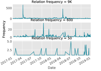
Figure 1: Distribution of three relations with different frequency over ICEWS Jan 2017-Jan 2019. The distribution of occurrences is highly heterogeneous.

Most of the existing KG completion methods rely on a sufficiently large number of training examples per relation. Unfortunately, most real-world KGs have a long-tail structure, so many relationships occur only a handful of times. Recent research has addressed the problem by developing efficient low-shot learning methods. Xiong et al. 2018 pioneered employing few-shot learning (FSL) to infer a link between two entities given only one training example, which is done by learning a matching metric over the embeddings extracted from the one-hop neighborhood of entities in the graph. Several followup works improving upon GMatching (Bose et al. 2019; Chen et al. 2019; Wang et al. 2019a, b) are also comprised of an encoder component extracting features for the meta learning component.

The data scarcity issue is exacerbated for temporal graphs, since the dynamic governing the evolution of those graphs might be highly non-stationary. First, new types of relationships/events might emerge that have not been observed before. Furthermore, even if a given relation has been observed frequently over some time interval, the distribution of occurrences over that interval might be highly inhomogeneous and bursty, as shown in Fig. 1. The existing methods, which are developed for static graphs, cannot account for such dynamics. First, their encoders are not able to incorporate the existing temporal dependencies between entities into the model. Second, their task definition in the FSL framework does not account for time constraints. Thus, we need novel low-shot learning approaches to accurately model TKGs.

We address this challenge by proposing a new model, Few-shot Temporal Attention Graph Learning (FTAG), to effectively infer the true entity pairs for a relation, given only one support entity pair. Our model learns a representations for entities by aggregating temporal information over neighborhoods. It employs a self-attention mechanism to sequentially extract an entity’s neighborhood information over time. Temporally adjacent events could convey useful information about the events that will happen in the future. Thus, self-attention, as a powerful tool for sequence modeling, has been used to extract a time-aware representation from the entity neighborhood. Then, the learned representation would be used to match a given support entity pair with a query entity pair and generate a similarity score proportional to the likelihood of the event.

Our contributions are summarized as follows:

• We introduce a one-shot learning framework for temporal knowledge graphs, which generalizes over existing low-shot techniques for static graphs.

• We propose a temporal neighborhood encoder with a self-attention mechanism that effectively extracts the temporally-resolved neighborhood information for each entity in the graph.

• We conduct extensive experiments with two popular real-world datasets and demonstrate the superiority of the proposed model over state of the art baselines.

• We construct two new publicly-available benchmarks for one-shot learning over temporal knowledge graphs.

2 Problem Formulation

We present the formal definition of a TKG and explore few-shot learning tasks for temporal link prediction.

2.1 Temporal Knowledge Graph Completion

A TKG can be represented as a set of quadruples $G=\{(s,r,o,t)|s,o\in\mathcal{E},r\in\mathcal{R}\}$, where $\mathcal{E}$ is the set of entities, $\mathcal{R}$ is the set of relations and $t$ is the timestamp. Graph completion for a static KG involves predicting new facts by either predicting an unseen object entity for a given subject and relation $(s,r,?)$ or predicting an unseen link between the subject and object entity $(s,?,o)$. In this work, we are interested in the former case, but at a particular timestamp $t$. More formally, we want to predict new events $(s,r,?,t)$ at time $t$ by ranking the true object entities higher than others by a scoring function $\mathcal{P}$, parameterized by a neural network and its value indicating the event likelihood. The key idea in modeling the temporal events is that an event likelihood depends on the events in the previous $\ell$ timesteps $\{t-\ell,\dots,t-2,t-1\}$. In Section 3.1 we explain in detail that how temporal information is encoded in our model.

2.2 Few-shot Learning and Episodic Training

Few-shot Learning (FSL) focuses on building and training a model with only a few labeled instances for each class. Meta-learning is a framework to address FSL where we incorporate a large set of tasks, and each task mimicks an N-way K-shot classification scenario. The aim is to leverage the shared information across the tasks to compensate for the scarcity of information about each task resulting from having few labeled data points.

The idea of episodic training for meta-learning is to match the training procedure with the inference at test time (Vinyals et al. 2016). More specifically, consider that we have a large set of tasks $\mathcal{T}$. Each episode consists of a subset of tasks $L$, sampled from $\mathcal{T}$, a support set $S$, and a batch $B$ both sampled from $L$. Note that both $S$ and $B$ are labeled examples, labels coming from $L$. The goal is to train a model that maps the few examples in the support set into a classifier. The probabilistic optimization objective for this problem can be formulated as:

$$\theta=\underset{\theta}{\operatorname*{arg\,max}}E_{L\sim\mathcal{T}}\Bigg{[}E_{S\sim L,B\sim L}\Bigg{[}\underset{(x,y)\in B}{\sum}\log P_{\theta}(y|x,S)\Bigg{]}\Bigg{]}.$$ (1)

We adopt the standard episodic training framework in Eq. (1) for the purpose of TKG completion.

2.3 Few-shot TKG Setup

As mentioned earlier, data scarcity is even a bigger problem in relational learning with TKGs. Few-shot episodic training has been proven to be effective to tackle this problem for static KGs (Xiong et al. 2018). We further extend the framework proposed by Xiong et al. 2018 for TKG completion.

Given a TKG, $G=\{(s,r,o,t)|s,o\in\mathcal{E},r\in\mathcal{R}\}$, the relations of $\mathcal{R}$ are divided into two groups based on their frequency: frequent relations $\mathcal{F}$ and sparse relations $\mathcal{T}$. The sparse relations are used to build the task set needed by the model for the episodic training. Each task is defined as a sparse relation $r\in\mathcal{T}$ and has its own training and test set, denoted as support and query set and defined as:

$$\begin{split}&S_{r}=\{(s_{0},r,o_{0},t_{0})|s_{0},o_{0}\in\mathcal{E}\}\\ &Q_{r}=\{(s_{q},r,o_{q},t_{q})|s_{q},o_{q}\in\mathcal{E}\},\end{split}$$ (2)

Where $S_{r}$ contains one labeled example. At each episode, one relation is selected at random and one quadruple containing that relation to form the support set. We can select the quadruples for the query set in two ways:

1. Random: At each episode, $m$ quadruples are selected randomly for the query set.

2. Time dependent: The quadruples of the query set are restricted by their distance from the support set timestamp:

   $$Q_{r}^{t}=\{(s_{q},r,o_{q},t_{q})|s_{q},o_{q}\in\mathcal{E},t_{q}\in[t_{0},t_{0}+w]\}$$ (3)

   Where $t_{0}$ is the support set timestamp. Figure 2(a) illustrates the time constraint used for selecting the query examples. More details on sampling procedure for the support and query set are provided in Section 3.3. The parameter $w$ is called the episode length.

The loss function $l_{\theta}$ at each episode optimizes a score function $\mathcal{P_{\theta}}$ such that for a given test query in $Q_{r}^{t}$, the true object entities are ranked higher than the others. The score function is a metric space learnt during the training, and the score represents the similarity between a test query and the support set representation. The final optimization loss is:

$$\mathcal{L}=E_{r\sim\mathcal{T}}\bigg{[}E_{Q_{r}^{t}\sim G,S_{r}^{t}\sim G}\bigg{[}l_{\theta}(Q_{r}^{t}|S_{r}^{t})\bigg{]}\bigg{]}$$ (4)

The relations in $\mathcal{T}$ are divided into mutually exclusive sets: $\mathcal{T}_{meta-train},\mathcal{T}_{meta-test},\mathcal{T}_{meta-val}$. From this, $meta_{train}$ is defined as:

$$meta_{train}=\{(s,r,o,t)|r\in\mathcal{T}_{meta-train}\}$$

$meta_{val}$ and $meta_{test}$ are defined similarly. To make the temporal setup more representative of the real world, we do not allow any time overlap between the quadruples in $meta_{train}$, $meta_{val}$ and $meta_{test}$. Figure 2(b) depicts the time split for $meta_{train}$, $meta_{val}$ and $meta_{test}$. To have the episodes in the training match with the inference, the split window for validation and test is equal to $w$.

(a) Query and support set construction

(b) Train, validation and test split across time

Figure 2: (a) The query set is selected from $[t_{i},t_{i}+w]$, with $t_{i}$ being the last quads timestamp in the support (b) There is no time overlap between quadruples in validation and test.

Finally, we assume that the model has access to a background knowledge graph defined as $G^{\prime}=\{(s,r,o,t)|s,o\in\mathcal{E},r\in\mathcal{F}\}$, and the entity set $\mathcal{E}$ is a closed set, i.e., there are no unseen entities during the inference time.

3 Model

(a) Neighborhood Encoder

(b) Similarity Network

Figure 3: Depiction of the main components of our model: (a) Temporal neighborhood encoder comprised of a snapshot encoder $f_{\eta}$ and the $Att$ modules; (b) Similarity score is computed via the inner product.

Our model is built upon two main fundamentals: (i) a representation for the support set and query instances to preserve the relational/sequential graph structure, and (ii) a metric to determine the similarity of the support set and a query instance. From this, our model consists of two main components (Figure 3), as follows:

Neighborhood Encoder. The neighborhood encoder represents the neighborhood information of a given entity $e$ as a $d$ dimensional vector $h_{e}$. It encodes the one-hop neighborhood structure during the past $\ell$ timesteps as a sequence. In Section 3.1 we explain the detail of obtaining a test query and support set representation via the encoder.

Similarity Network. A similarity function parameterized by a neural network, $\mathcal{M}(q,S))$, that outputs a scalar similarity score between the query instance $q$, and the support set $S$, where $q=(s_{q},r,o_{q},t)$ is a potential event and the similarity score is proportional to the likelihood of that event.

3.1 Neighborhood Encoder

For a given entity $e$, we define $\mathcal{N}^{r}_{\tau}(e)$ as the set of all adjacent entities connected to $e$ with relation $r$ at time $\tau$, and the temporal neighborhood $N(e)=\bigcup_{r\in\mathcal{F},\tau\in[t-\ell,t-1]}N^{r}_{\tau}(e)$. The neighborhood encoder is comprised of two parts: (i) function $f_{\eta}$ that encodes the one-hop neighborhood at a given timestamp $\tau$, and (ii) function $g$, that utilizes the output of function $f_{\eta}$, at previous timesteps, to generate a temporal neighborhood representation.

Snapshot Aggregation.

The snapshot aggregator $f_{\eta}$ aggregates local neighborhood information at a specific time $\tau$.

$$\begin{split}&f_{\eta}(N_{\tau}(e))=\\ &\sigma(\frac{1}{C_{e_{\tau}}}\sum_{r\in\mathcal{F}}\sum_{e_{j}\in N^{r}_{\tau}(e)}(W^{T}[v_{r}:v_{e_{j}}]+b))\\ &x_{\tau}^{e}=[f_{\eta}(N_{\tau}(e)):v_{e}],\end{split}$$ (5)

where $C_{e_{\tau}}$ is a normalizing factor, $v_{e_{j}}\in\mathbf{R}^{d\times 1}$, $v_{r}\in\mathbf{R}^{d\times 1}$are entity and relation representations, and $W\in\mathcal{R}^{2d\times d}$ and $b\in\mathcal{R}^{d\times 1}$ are model parameters to be learnt. $\sigma(.)$ is a nonlinear activation function ($Relu$ in our case).

Sequential Aggregation

Function $g$ aggregates the sequence of snapshots from previous $l$ timesteps $\{t-\ell,\dots,t-2,t-1\}$. We then use a transformer, as proposed in (Vaswani et al. 2017). This is an encoder-decoder model solely based on attention mechanism that proves to be powerful for modeling sequential data. Here, the encoder part, denoted as Att, is employed to effectively capture the time dependencies between the event sequences. The main component of Att function is a layer, made up of two sublayers:

Attention sublayer projects the input sequence to a query and a set of key-value vectors.

$$\begin{split}&\textrm{MultiHead}(Q,K,V)=[head_{1}:...:head_{h}]W^{O}\\ &head_{i}=\textrm{Attention}(QW_{i}^{Q},KW_{i}^{K},VW_{i}^{V}),\end{split}$$ (6)

where $W_{i}^{Q}\in\mathbf{R}^{d_{model}\times d_{k}}$ , $W_{i}^{K}\in\mathbf{R}^{d_{model}\times d_{k}}$ , $W_{i}^{V}\in\mathbf{R}^{d_{model}\times d_{v}}$, $W^{O}\in\mathbf{R}^{hd_{v}\times d_{model}}$ are parameter matrices, and $d_{model}$ is the input embedding dimension ($d_{model}=2d$ in our case).

Position wise sublayer is a fully connected feed-forward network, applied to each sequence position separately and identically.

$$FFN(x_{\tau})=\max(0,x_{\tau}W_{1}+b_{1})W_{2}+b_{2}.$$ (7)

The $\textit{Att}(x,n_{head},n_{layer})$ takes as input a sequence of neighborhood snapshot representations $x=\{x^{e}_{t-\ell},\dots,x^{e}_{t-1}\}$, the number of layers, and number of attention heads, and maps input sequence $x$ to a time-aware sequence output $z=[z_{t-\ell},\dots,z_{t-1}]$ as follows:

$$z=\textit{Att}(x,n_{head},n_{layer}))$$ (8)

Finally, the temporal neighborhood representation for $e$ at time $t$ is obtained by:

$$h_{e}=\sigma([z_{t-\ell}:\dots:z_{t-1}]W^{*}),$$ (9)

where $W^{*}\in\mathbf{R}^{2dl\times d_{out}}$ is a parameter matrix, $[:]$ is concatenation and $\sigma(.)$ is a nonlinear activation function ($Relu$ in our case). More detail on Att is provided in Appendix A.

3.2 Similarity Network

Given the Neighborhood encoder, every pair of subject and object $(s,o)$ can be represented as a vector $[h_{s}:v_{s}:h_{o}:v_{o}]$, where $h_{s}$ and $h_{o}$ are the temporal representations obtained from the neighborhood encoder and $v_{s}$ and $v_{o}$ are the embeddings for the subject and the object entities.

Given the support entity pair $(s_{0},o_{0})$ for a relation $r$, we learn the representation for similarity from the support and the query entity pair by two layers of fully connected layers:

$$\begin{split}&x^{(1)}=\sigma(W^{(1)}x+b^{(1)})\\ &x^{(2)}=W^{(2)}x^{(1)}+b^{(2)}\\ &\mathcal{M}(x)=x^{(2)}+x.\end{split}$$ (10)

The inner product is used to compute the similarity score between the support and query entity pair:

$$score=\mathcal{M}(s)^{T}.\mathcal{M}(q),$$ (11)

where $s=[h_{s_{0}}:v_{s_{0}}:h_{o_{0}}:v_{o_{0}}]$ and $q=[h_{s_{q}}:v_{s_{q}}:h_{o_{q}}:v_{o_{q}}]$. We use the dot product to output a similarity score between the support and query pair that corresponds to the likelihood of $s_{q}$ and $o_{q}$ being connected with $r$.

	GDELT				ICEWS
Model	H@1	H@5	H@10	MRR	H@1	H@5	H@10	MRR
TTransE	0.025	0.075	0.138	0.060	0.004	0.047	0.107	0.038
TATransE	0.062	0.200	0.362	0.151	0.084	0.238	0.418	0.168
ReNet	0.064	0.191	0.319	0.146	0.126	0.289	0.407	0.209
GMatching	0.007	0.037	0.067	0.028	0.062	0.156	0.233	0.113
FSRL	0.080	0.158	0.210	0.127	0.120	0.253	0.345	0.192
MetaR	.0.003	0.235	0.293	0.115	0.044	0.172	0.244	0.112
FTAG (Random)	0.228	0.416	0.525	0.331	0.191	0.479	0.641	0.325
FTAG (Time dependent)	0.234	0.441	0.578	0.345	0.170	0.519	0.743	0.323

Table 1: Hit@K results for one-shot learning on (i) one month of GDELT (Jan $2018$) and (ii) two years of ICEWS (Jan $2017$ - Jan $2019$) for relations in $\mathcal{T}_{meta-test}$. “Random” and “Time dependent” correspond to the query set selection method.

3.3 Loss Function and Training

Algorithm 1

function MakeTask($r,w,A_{r},n_{shots}$)

     $i\sim\textrm{Uniform}(1,|A_{r}|)$

     $S_{r}^{t}\leftarrow\{A_{r}[i]\}$

     $limit\leftarrow w+t_{j+1}$

     while $t_{j}<limit$ do

         Add $A_{r}[j]$ to $Q_{r}^{t}$

         $j\leftarrow j+1$      

     return $S_{r}^{t}$, $Q_{r}^{t}$

Input:

1: Meta training relations $\mathcal{T}$

2: $\forall r,A_{r}=\{(s_{i},r,o_{i},t_{i})\}$ $\triangleright$ $t_{i}$ are sorted

3: Background TKG $G^{\prime}$

4: Episode length $w$, Number of shots $n_{shots}$

for $i=1,2,\ldots N$ do

     Shuffle relations in $\mathcal{T}$

     Sample relation $r$ from $\mathcal{T}$

     $S_{r}^{t},Q_{r}^{t}\leftarrow$ MakeTask($r,w,A_{r},n_{shots}$)

     Sample $B^{+}$ from $Q_{r}^{t}$ and make $B^{-}$

     $\mathcal{L}\leftarrow\max(score^{-}-score^{+}\lambda,0)$

     $\theta\leftarrow\theta-\nabla\mathcal{L}$

return $\theta$

For a given relation $r$ and its support set $S_{r}^{t}=\{(s_{0},r,o_{0},t)\}$, we have a set of positive quadruples ($Q_{r}^{t^{+}}$) and construct the negative pairs ($Q_{r}^{t^{-}}$) by polluting the subject or object entities for each positive quadruple and the final query set is $Q_{r}^{t}=Q_{r}^{t^{-}}\bigcup Q_{r}^{t^{+}}$. We want the positive quadruples to be close to the final representation of the support set and the negatives to be as far as possible. The objective function that we optimize is a hinge loss, defined as:

$$\mathcal{L}=max(score^{-}-score^{+}+\lambda,0)$$ (12)

The $score^{+}$ and $score^{-}$ are similarity scores calculated over $Q_{r}^{t^{+}}$ and $Q_{r}^{t^{-}}$. We employ episodic training over the task set $\mathcal{T}$ to optimize the loss function. Algorithm 1 summarizes the time dependent selection to construct the query set and the episodic training algorithm.

4 Experiments

We evaluate our model on predicting new events for a relation by predicting the object entity $(s,r,?,t)$ and conduct qualitative and quantitative experiments on the model. This section includes the details of dataset and task construction, the proposed baselines, performance comparison and ablation studies on variations of our model.

4.1 Datasets

We use two datasets: Integrated Crisis Early Warning System (ICEWS) (Boschee et al. 2015) and Global Database of Events, Language, and Tone (GDELT) (Leetaru and Schrodt 2013). ICEWS and GDELT are two widely-used benchmarks for TKG completion tasks. Both are large geopolitical event datasets automatically extracted and coded from news archives. In both datasets, the CAMEO-coding scheme is used to represent the events. CAMEO codes are a set of predefined geopolitical interactions that constitute knowledge graph relations. Each dyadic event is represented as a timed interaction (CAMEO code) between two geopolitical actors (knowledge graph entities). ICEWS is updated on a daily basis and GDELT every 15 minutes. From these datasets, we construct two new benchmarks for one-shot relational learning over TKGs.

Our first dataset is constructed from two years of the ICEWS dataset, from Jan 2017 to Jan 2019. Events timestamps have daily granularity in ICEWS. We select the relations with frequency between 50 and 500 for the one-shot learning tasks and frequency higher than 500 as the background relations. Our second dataset includes one month of GDELT (Jan 2018). GDELT is much larger than ICEWS, since it is updated every 15 minutes, and the event timestamps have 15 minutes granularity. The low and high frequency thresholds for selecting tasks and background relations are 50 and 700, respectively, for the GDELT dataset. The rest of the dataset pre-processing is the same for both GDELT and ICEWS. Table 2 shows the statistics for both datasets.

Dataset	$\#$ Ents	$\#$ Rels	$\#$ Tasks	$\#$ Quads
ICEWS	2419	153	66/5/14	7535
GDELT	1549	204	50/5/14	10420

Table 2: Dataset statistics for two years of ICEWS($2017$-$2019$) and one month of GDELT (Jan 2018).$\#$Rels include all the meta relations and background relations, and $\#$Tasks is the number of relations in $\mathcal{T}_{meta-train}/\mathcal{T}_{meta-val}/\mathcal{T}_{meta-test}$.

	Setting			GDELT			ICEWS
Model	Att	Rand	MatchNet	H@1	H@10	MRR	H@1	H@10	MRR
M1				0.045	0.225	0.114	0.060	0.558	0.197
M2				0.133	0.504	0.243	0.105	0.518	0.220
M3				0.197	0.535	0.293	0.123	0.616	0.245
M4				0.169	0.491	0.265	0.138	0.654	0.269
FTAG (Random)				0.228	0.525	0.331	0.191	0.641	0.325
FTAG (Time dependent)				0.234	0.578	0.345	0.170	0.743	0.323

Table 3: Ablation study on different components of the model (i) one month of GDELT (Jan 2018) and (ii) two years of ICEWS (Jan 2017 - Jan 2019) for relations in $\mathcal{T}_{meta-test}$.

4.2 Baselines

There is no prior work on one-shot learning for temporal knowledge graphs. Therefore, we propose two different ways to evaluate our model:

1. One-shot training of existing TKG models To simulate the one-shot condition, we make a training set by adding all the quadruples of the background knowledge graph, as well as the quadruples of the meta-train. Per each relation in the meta-test and meta-val, we also include exactly one quadruple into the training set. We test the model on the exact same quadruples from meta-test. The TKG reasoning models used as baseline include: TADistMult (Garcia-Duran, Dumančić, and Niepert 2018), TTransE (Leblay and Chekol 2018) and ReNet (Jin et al. 2019).

2. FSL methods for static graphs: We collapse the temporal training graph into an unweighted static graph. An edge exists between two entities in the static graph if there is a corresponding edge in the temporal graph at any time. We use three state of the art static low-shot learning methods: GMatching (Xiong et al. 2018), FSRL (Zhang et al. 2020a), and MetaR (Chen et al. 2019). Unlike the first two, MetaR doesn’t incorporate any neighborhood information into its modeling, meaning that there is no difference between $(s,r,o,t_{i})$ and $(s,r,o,t_{j})$ in the test. In contrast, the one-hop neighborhood information provided for $(s,r,o,t_{i})$ is different than $(s,r,o,t_{j})$ during the test time of GMatching and FSRL.

4.3 Evaluation

We divide the dataset into train, validation, and test splits, as explained in Section 2.3 and visualized in Figure 2(b). We evaluate the models using Hit@(1/5/10) and Mean Reciprocal Rank (MRR). We use all the entities in the dataset to generate a list of potential candidates for ranking. For each method, the model with the best MRR on the validation set is selected for evaluation over the test set. Table 1 summarizes the results of prediction tasks on the ICEWS and GDELT datasets. The one-shot support example for $\mathcal{T}_{meta-test}$ is selected from the training period for the first set of baselines. For our method and the second set of baselines, it is possible to select a one-shot example from the test period. We also tested our method with the same one-shot example provided to the first three baselines, selected from the training period, but the difference was not significant. We run each method five times with a different random seed and report the average. Appendix B includes the details of hyperparameter selection and implementation.

Discussion. We observe in Table 1 that our model outperforms all the baselines. In particular, the improvement is significant for Hit@10. The episodic training used in our model provides more generalizability compared to the first set of baselines that use regular training. Our initial experiments show that the performance of these models are closer to the frequent relations and declines when evaluated over only sparse relations. Although the second set of baselines employ episodic training, these methods still fail to consider the temporal dependency between events, which is captured effectively by self-attention in our model.

4.4 Ablation Study

To demonstrate the importance of each component of our model, we conduct multiple ablation studies that evaluate the model from three main angles:

1. The temporal neighborhood encoder added by self-attention to the model: We disable the sequential encoder and feed all the neighbors of an entity in $\{t-\ell,\dots,t-1\}$ to the snapshot function $f_{\eta}$, as if they all happened at one timestamp (M1), shown in Table 3 as “Att”.

2. Query set selection method: According to Section 2.3, it can either be random or time dependent. “Rand” is checked in Table 3 if the selection method is random, and time dependent otherwise.

3. We analyze the effectiveness of the inner product to a more complicated model and add Matching Network (Xiong et al. 2018) to the query representation. It is shown as “MatchNet” in Table 3.

Table 3 summarizes the ablation study’s results, showing that the full pipeline of our proposed algorithm outperforms the other variations. M1 and M2 show the effectiveness of a sequential encoder, since disabling it cause a significant decline in the performance. It is worth noting that adding MatchNet helps to capture similarity information when the model is simple (M1 and M2). However, comparing FTAG/FTAG-R with M3 and M4 shows that, due to the lack of data, adding MatchNet will lead to overparameterizing the model and decreasing the performance, while self-attention is powerful enough to learn a representation that captures not only the temporal dependencies but also a similarity space that enables accurate prediction.

4.5 Performance Over Different Relations

In this section, we conduct experiments to evaluate the model performance over each relation separately. Table 4 shows relations in ICEWS test set by performance. Our model struggles on CAMEO codes “1831” and “1823,” which lie under a higher level CAMEO event “Assault” coded as “18.” Also, we manually inspected the test examples for “1823,” for which ReNet performs very well. Our inspection shows that ReNet tends to generate higher ranks for a quadruple $(s,r,o,t)$ if it has already seen many examples of $s$, $o$ being paired with any other relations. For example, (ISIS, 1831, Afghanistan) was the test example, and we found 30 matches for (ISIS, 183, Afghanistan) in the training set. It is worth noting that “1831” is a subcategory of “183” in the CAMEO-code scheme. This was the case for 4 out of 5 query examples of “1831.” The one query example that ReNet doesn’t perform well, (ISIS, 1831, Libya), the combination of $ISIS$ and any other $Libya$ related entities only appeared 7 times in the training data. The rank predicted by our model for this query is 14, while the ReNet rank is over 1,000. Our model doesn’t use the information from the edges in the background graph. Although ReNet leverages this information, it could become biased toward them. Therefore, designing a few-shot model that leverages this information and is able to generalize well over new edges remains a challenge for future work.

4.6 Performance over Time

Figure 4 visualizes the performance of our model over time for ICEWS dataset. Since relations selected for the task are very sparse, the number of query examples in one unit of time is very small. So we aggregated every 7 days. The y axis is the time difference between the query timestamp and its support example timestamp. Figure 4 shows that our model outperforms the best baseline over time.

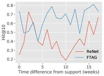
Figure 4: Model performance as the time between the prediction and the end date of the support set increases.

		Hit@10
CAMEO Code	Frequency	FTAG	ReNet
1044	52	0.300	0.600
1125	58	0.650	0.615
1311	64	0.567	0.000
186	71	0.533	0.250
1831	97	0.450	0.800
1122	121	0.757	0.667
011	128	0.600	0.000
0313	130	0.656	0.579
1823	143	0.133	0.286
1721	225	0.600	0.133
0312	273	0.800	0.714
063	283	0.688	0.364
0333	292	0.612	0.353
0332	348	0.785	0.463

Table 4: Hit@10 and MRR reported separately for each relation in the test tasks for ReNet and FTAG. The description of CAMEO codes is provided in Appendix E.

5 Related Work

Our work is particularly related to representation learning for temporal relational graphs, few-shot learning methods and recent developments of meta learning approaches for graphs.

Few-Shot Learning. An effective approach for few-shot learning is based on learning a similarity metric and a ranking function using training triples (Koch, Zemel, and Salakhutdinov 2015; Vinyals et al. 2016; Snell, Swersky, and Zemel 2017; Mishra et al. 2018). Siamese networks (Koch, Zemel, and Salakhutdinov 2015) use a pairwise loss to learn a metric between input representations in an embedding space and then use the learnt metric to perform nearest-neighbours separately. Matching networks (Vinyals et al. 2016) learn a function to embed input features in a low-dimensional space and then use cosine similarity in a kernel for classification. Prototypical networks (Snell, Swersky, and Zemel 2017) compute a prototype for each class in an embedding space and then classify an input using the distance to the prototypes in the embedding. SNAIL (Mishra et al. 2018) uses temporal convolution to aggregate information from past experiences and causal attention layers to select important information from past experiences. Another paradigm of few-shot learning includes optimization-based approaches that usually include a neural network to control and optimize the parameters of the main network. One example is MAML (Finn, Abbeel, and Levine 2017) that learns how to generalize with only a few examples and doing a few gradient updates.

Relation Learning for TKGs. The temporal nature of TKGs introduces a new piece of information, as well as a new challenge in learning representation for TKGs. To model the time information (Leblay and Chekol 2018; Garcia-Duran, Dumančić, and Niepert 2018; Dasgupta, Ray, and Talukdar 2018) embed the corresponding time by: encoding the time text by an RNN (Garcia-Duran, Dumančić, and Niepert 2018), low dimensional embedding vectors (Leblay and Chekol 2018) and hyper planes (Dasgupta, Ray, and Talukdar 2018). Other methods try to capture the temporal entities’ interactions by encoding them with a sequential model, such as (Trivedi et al. 2017) that represents events as the point processes, and (Jin et al. 2019) that aggregates the one-hop entity neighborhood at each timestamp by a pooling layer, and pass it to an RNN in an auto-regressive manner.

Few-shot Learning for Graphs. Few-shot learning for graphs has recently gained attention. Xiong et al. (Xiong et al. 2018) pioneered and proposed a few-shot learning framework for link prediction over the infrequent relations. They extract a representation for each entity from its one-hop neighborhood and learn a common similarity metric space. A number followup studies also combine local neighborhood structure (Zhang et al. 2020a; Du et al. 2019) or reasoning paths (Wang et al. 2019a; Lv et al. 2019) with a meta learning algorithm, such as MAML. Chen et al. (Chen et al. 2019) leverage the same framework, although they don’t use the local neighborhood structure. An adversarial procedure is used by Zhou et al. (Zhang et al. 2020b) to adopt features from high to low resource relations. Wang et al. (Wang et al. 2019b) extend the effort from infrequent relations to tackle the unpopular entities problem in KGs by integrating textual entity descriptions. Meta-Graph (Bose et al. 2019) is a gradient-based meta learning approach for graphs. It leverages higher-order gradients along with a learned graph signature function to generates a graph neural network initialization. These approaches all assume a static graph. To the best of our knowledge, we are the first to study few-shot learning for temporal knowledge graphs.

6 Conclusion and Future Work

We introduce a novel one-shot learning framework for temporal knowledge graphs to address the problem of infrequent relations in those graphs. Our model employs a self-attention mechanism to sequentially encode temporal dependencies among the entities, as well as a similarity network for assessing the similarity between a query and an example. Our experiments demonstrate that the proposed method outperforms existing state-of-the-art baselines in predicting new events for infrequent relations. In future work, we would like to generalize the current one-shot learning to a few-shot scenario. Another direction is extending our framework to handle emergent entities, a challenge since new entities will have fewer interactions and thus considerably sparser neighborhood information.

Appendix A Attention Encoder Details

The Attention function used in Equation 6 to calculate the attention score is called “Scaled Dot Product Attention” in (Vaswani et al. 2017) and defined as follows:

$$\textrm{Attention}(Q,K,V)=softmax\big{(}\frac{QK^{T}}{\sqrt{d_{k}}}\big{)}V$$ (13)

In order for the attention model to make use of sequential order, a positional encoding is added to the input embeddings.

$$\begin{split}&PE_{(pos,2i)}=sin(pos/10000^{2i/d_{model}})\\ &PE_{(pos,2i+1)}=cos(pos/10000^{2i/d_{model}}),\end{split}$$ (14)

Where $pos$ is the position and $i$ is the dimension. The purpose of positional encoding is to introduce to the model the information about relative or absolute position of each element in the sequence. The positional encoding has similar dimension as $d_{model}$.

Appendix B Hyperparameters

We select the relations with frequency between 50 and 500 for the one-shot learning tasks and frequency higher than 500 as the background relations for ICEWS dataset. The low and high frequency thresholds for selecting tasks and background relations are 50 and 700, respectively, for the GDELT dataset.The threshold for choosing the sparse relations should be selected such that the sparsity is preserved and also, we have enough data for training the model. We have selected the exact threshold values based on the prior work (Xiong et al. 2018) which also is based on the above rationale. GDELT is less sparse than ICEWS, so we increased the upper threshold to increase the number of tasks for the training.
We use a manual tuning approach to select the model hyperparameters, during which we keep all the parameters constant except one and we run the model with the selected hyperparameters 5 times and select the best model over the validation set using MRR metric.
The episode length $w$ chosen to construct the datasets for one-shot learning from GDELT and ICEWS is 120 time units (e.g. 120 days for ICEWS). The history period is 20 days for ICEWS and 10 time units (every 15 minutes) for GDELT. The embedding size for both datasets is $50$. We use one layer of multi-head attention with 4 heads. Number of heads is selected by hyperparameter search from 1 to 6. Attention inner dimension is 256. Attention parameters are similar for both datasets. The matching network performs 3 steps of matching. The loss margin is 10 for ICEWS and 18 for GDELT. We found out that increasing margin value affects the performance as it is depicted in Figure 5. The number of parameters for the model with this choice of hyperparameters is 1,380,656 for GDELT dataset and 1,469,056 for ICEWS. We use Adam optimizer with initial learning rate 0.001.

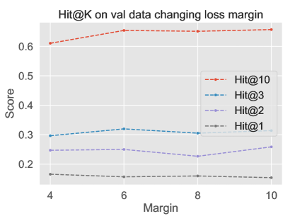
Figure 5: Model performance vs. the margin parameter.

Appendix C Model Selection

During model selection, we noticed that there is a trade off between optimizing Hit@K for the smaller versus higher $K$. MRR favors smaller $K$ because smaller ranks contribute more to MRR. So using MRR for model selection results in a model with higher HIT@1. Figure 6 show FTAG and ReNet performance for different $K$, with Hit@10 and MRR being used as the model selection metric. For ReNet, the validation set contains all the relations in the training set. This means that a model with the best Hit@10 doesn’t necessarily give the best Hit@10 over $\mathcal{T}_{meta-val}$. We also tried using the same validation set as our model, that only contain $\mathcal{T}_{meta-val}$. This resulted in lower accuracy and higher variance for ReNet.

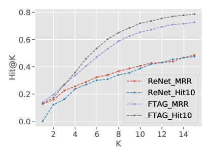
Figure 6: Hit@K for various values of K.

Appendix D Model Analysis

In this section we provide more insights on the shortcoming of the existing baselines and the justification about why our model outperforms these models. We compare our model against two categories of baselines:
TKG baselines: Regular TKG methods tend to get biased toward the frequent relations. We conducted some initial experiments to confirm it; We provided a training set containing all the relations to the model, and evaluated it on all the relations as well as sparse/frequent relations separately. The model performance (MRR/Hit@K) over all the relations was more close to the MRR/Hit@K for frequent relations and the MRR/Hit@K for sparse relations was much lower. The main difference between regular TKG models and our model is the episodic training framework, which enables our model to generalize well from only one example.

• TTransE/TATransE are translation based models which are not able to handle one-to-many/many-to-one relations. they map the timestamp in a quadruple (s, r, o, t) into a lower dimensional space and are not capable of extrapolation (i.e. forecasting the future events).

• ReNet: Same as our model, ReNet generates a time-aware representation for an entity by aggregating the local neighborhood at each timestamp using a pooling layer and feeding it to an RNN. In Section 4.5 we provide some insight on why and when the ReNet model outperforms our model.

FSL baselines:The main difference between our model and static FSL models is a temporal neighborhood aggregator. Temporal adjacent events could convey useful information about the events that will happen in the future and different timestamps can have different effects on future events. The multi-head self-attention module in our model captures this information. We did some experiments on history length that indicated that as we increased the history length upto some point, it helped to improve the model performance.

• GMatching uses a mean pooling layer to aggregate the entities and edges adjacent to the given entity.

• FSRL uses a weighted mean pooling layer with attention weights. The reason that FSRL works better than GMatching might be that a part of the temporal information is captured by attention weights.

• MetaR does not use the local neighborhood structure for extracting the embedding of a node.

To summarize, our model combines the benefits of both approaches: a self-attention to encode the temporal neighborhood information and a temporal task definition for episodic training, resulting in better performance over the baselines.

Appendix E CAMEO Code Description

Code	Description
1044	Demand change in institutions, regime
1125	Accuse of espionage, treason
1311	Threaten to reduce or stop aid
185	Assassinate
1831	Carry out suicide bombing
1122	Accuse of human rights abuses
011	Decline comment
0313	Express intent to cooperate on judicial matters)
1823	Kill by physical assault
1721	Impose restrictions on political freedoms
0312	Express intent to cooperate militarily
063	Engage in judicial cooperation
033	Express intent to provide humanitarian aid
0332	Express intent to provide military aid

Table 5: Mapping from CAMEO code to description.

Appendix F Implementation Detail

We implemented our solution using Pytorch. We run all the experiments on a CPU Intel(R) Xeon(R) Gold 5220 CPU @ 2.20GHz, and 53 GBs of memory. The eval function in trainer.py includes the details to calculate MRR and Hit@K metrics. The implementation and the dataset is available at https://github.com/AnonymousForReview

Appendix G Data Construction

We provide the details of two newly constructed baselines for one-shot learning over temporal knowledge graphs. We conducted the following steps over both GDELT and ICEWS dataset:

1. A pre-processing step to deduplicate the dataset records by Source Name (subject), Target Name (object), CAMEO Code (relation), and Event Date (timestamp).

2. We divide the relations into two groups: frequent and sparse by their frequency of occurrence in the main dataset. Relations occurring between 50 and 500 in ICEWS, and 70 and 700 for GDELT are considered “sparse.” Those occurring more than 500 times in ICEWS and more than 700 times in GDELT are considered frequent.

3. The quadruples of the main dataset are then split into two groups based on their relations. The quadruples containing frequent relations make background knowledge graph kept in pretrain.csv, and the quadruples containing sparse relations are kept for meta learning process (meta quadruples) kept in fewshot.txt

4. From the sparse relations, 5 are selected for meta-validation, 15 for meta-test and rest kept for meta-training.

5. We split the meta quadruples into meta-train, meta-validation, and meta-test not only based on their relations, but also based on the non-overlapping time split explained in Figure 2(b) of the paper.

Data Format Description

Each constructed dataset contains the following files: symbols2id.pkl. A dictionary containing ent2id, rel2id, and dt2id, which are the mapping from entities, relations and dates to IDs respectively.

id2symbol.pkl. A reverse mapping from IDs to symbols.

data2id.csv. A file containing all the quadruples after the deduplication step. The symbols are represented by their ids.

pretrain.csv. Contains the quadruples of the background knowledge graph.

fewshot.txt. Contains the meta quadruples in text format. Each line is a tab separated quadruple with the order $s,r,o,t$.

meta_train.pkl. A mapping from relations to meta quadruple IDs containing that relation. A quadruple ID indicates the line number corresponding to that quadruple in fewshot.txt. meta_test.pkl and meta_val.pkl are also created similarly, using meta-validation and meta-test relations.

hist_l_n. A folder containing the entities’ neighborhood information, with a maximum of $n$ neighbors at each snapshot and history length $l$. It includes the following files:

hist_o.pkl. The object neighborhood of meta quadruples in the fewshot.txt. The $i_{th}$ record corresponds to the quadruple in $i_{th}$ line of fewshot.txt.

hist_s.pkl. The subject neighborhood of meta quadruples in the fewshot.txt. The $i_{th}$ record corresponds to the quadruple in $i_{th}$ line of fewshot.txt.

.

References

- Boschee et al. (2015) Boschee, E.; Lautenschlager, J.; O’Brien, S.; Shellman, S.; Starz, J.; and Ward, M. 2015. Integrated Crisis Early Warning System (ICEWS) Coded Event Data. URL: https://dataverse. harvard. edu/dataverse/icews .
- Bose et al. (2019) Bose, A. J.; Jain, A.; Molino, P.; and Hamilton, W. L. 2019. Meta-Graph: Few shot Link Prediction via Meta Learning. arXiv preprint arXiv:1912.09867 .
- Chen et al. (2019) Chen, M.; Zhang, W.; Zhang, W.; Chen, Q.; and Chen, H. 2019. Meta Relational Learning for Few-Shot Link Prediction in Knowledge Graphs. In Proceedings of the 2019 Conference on Empirical Methods in Natural Language Processing and the 9th International Joint Conference on Natural Language Processing (EMNLP-IJCNLP), 4208–4217.
- Dasgupta, Ray, and Talukdar (2018) Dasgupta, S. S.; Ray, S. N.; and Talukdar, P. 2018. Hyte: Hyperplane-based temporally aware knowledge graph embedding. In Proceedings of the 2018 Conference on Empirical Methods in Natural Language Processing, 2001–2011.
- Du et al. (2019) Du, Z.; Zhou, C.; Ding, M.; Yang, H.; and Tang, J. 2019. Cognitive Knowledge Graph Reasoning for One-shot Relational Learning. arXiv preprint arXiv:1906.05489 .
- Finn, Abbeel, and Levine (2017) Finn, C.; Abbeel, P.; and Levine, S. 2017. Model-agnostic meta-learning for fast adaptation of deep networks. In Proceedings of the 34th International Conference on Machine Learning-Volume 70, 1126–1135.
- Garcia-Duran, Dumančić, and Niepert (2018) Garcia-Duran, A.; Dumančić, S.; and Niepert, M. 2018. Learning Sequence Encoders for Temporal Knowledge Graph Completion. In Proceedings of the 2018 Conference on Empirical Methods in Natural Language Processing, 4816–4821.
- Jin et al. (2019) Jin, W.; Jiang, H.; Qu, M.; Chen, T.; Zhang, C.; Szekely, P.; and Ren, X. 2019. Recurrent event network: Global structure inference over temporal knowledge graph. arXiv: 1904.05530 .
- Kasneci et al. (2009) Kasneci, G.; Ramanath, M.; Suchanek, F.; and Weikum, G. 2009. The YAGO-NAGA approach to knowledge discovery. ACM SIGMOD Record 37(4): 41–47.
- Koch, Zemel, and Salakhutdinov (2015) Koch, G.; Zemel, R.; and Salakhutdinov, R. 2015. Siamese neural networks for one-shot image recognition. In ICML deep learning workshop, volume 2. Lille.
- Leblay and Chekol (2018) Leblay, J.; and Chekol, M. W. 2018. Deriving validity time in knowledge graph. In Companion Proceedings of the The Web Conference 2018, 1771–1776. International World Wide Web Conferences Steering Committee.
- Leetaru and Schrodt (2013) Leetaru, K.; and Schrodt, P. A. 2013. GDELT: Global data on events, location, and tone. In ISA Annual Convention. Citeseer.
- Lv et al. (2019) Lv, X.; Gu, Y.; Han, X.; Hou, L.; Li, J.; and Liu, Z. 2019. Adapting Meta Knowledge Graph Information for Multi-Hop Reasoning over Few-Shot Relations. In Proceedings of the 2019 Conference on Empirical Methods in Natural Language Processing and the 9th International Joint Conference on Natural Language Processing (EMNLP-IJCNLP), 3367–3372.
- Mishra et al. (2018) Mishra, N.; Rohaninejad, M.; Chen, X.; and Abbeel, P. 2018. A Simple Neural Attentive Meta-Learner. In ICLR.
- Nickel et al. (2016) Nickel, M.; Murphy, K.; Tresp, V.; and Gabrilovich, E. 2016. A Review of Relational Machine Learning for Knowledge Graphs. Proceedings of the IEEE 1(104): 11–33.
- Snell, Swersky, and Zemel (2017) Snell, J.; Swersky, K.; and Zemel, R. 2017. Prototypical networks for few-shot learning. In Advances in Neural Information Processing Systems, 4077–4087.
- Trivedi et al. (2017) Trivedi, R.; Dai, H.; Wang, Y.; and Song, L. 2017. Know-evolve: Deep temporal reasoning for dynamic knowledge graphs. In Proceedings of the 34th International Conference on Machine Learning-Volume 70, 3462–3471. JMLR. org.
- Vaswani et al. (2017) Vaswani, A.; Shazeer, N.; Parmar, N.; Uszkoreit, J.; Jones, L.; Gomez, A. N.; Kaiser, Ł.; and Polosukhin, I. 2017. Attention is all you need. In Advances in neural information processing systems, 5998–6008.
- Vinyals et al. (2016) Vinyals, O.; Blundell, C.; Lillicrap, T.; Wierstra, D.; et al. 2016. Matching networks for one shot learning. In Advances in neural information processing systems, 3630–3638.
- Vrandečić and Krötzsch (2014) Vrandečić, D.; and Krötzsch, M. 2014. Wikidata: a free collaborative knowledgebase. Communications of the ACM 57(10): 78–85.
- Wang et al. (2019a) Wang, H.; Xiong, W.; Yu, M.; Guo, X.; Chang, S.; and Wang, W. Y. 2019a. Meta Reasoning over Knowledge Graphs. arXiv preprint arXiv:1908.04877 .
- Wang et al. (2019b) Wang, Z.; Lai, K.; Li, P.; Bing, L.; and Lam, W. 2019b. Tackling Long-Tailed Relations and Uncommon Entities in Knowledge Graph Completion. In Proceedings of the 2019 Conference on Empirical Methods in Natural Language Processing and the 9th International Joint Conference on Natural Language Processing (EMNLP-IJCNLP), 250–260.
- Wang et al. (2018) Wang, Z.; Lv, Q.; Lan, X.; and Zhang, Y. 2018. Cross-lingual knowledge graph alignment via graph convolutional networks. In Proceedings of the 2018 Conference on Empirical Methods in Natural Language Processing, 349–357.
- Xiong et al. (2018) Xiong, W.; Yu, M.; Chang, S.; Guo, X.; and Wang, W. Y. 2018. One-Shot Relational Learning for Knowledge Graphs. In Proceedings of the 2018 Conference on Empirical Methods in Natural Language Processing, 1980–1990.
- Yao and Van Durme (2014) Yao, X.; and Van Durme, B. 2014. Information extraction over structured data: Question answering with freebase. In Proceedings of the 52nd Annual Meeting of the Association for Computational Linguistics (Volume 1: Long Papers), 956–966.
- Zhang et al. (2020a) Zhang, C.; Yao, H.; Huang, C.; Jiang, M.; Li, Z.; and Chawla, N. V. 2020a. Few-Shot Knowledge Graph Completion. In International Joint Conference on Artificial Intelligence.
- Zhang et al. (2020b) Zhang, N.; Deng, S.; Sun, Z.; Chen, J.; Zhang, W.; and Chen, H. 2020b. Relation Adversarial Network for Low Resource Knowledge Graph Completion. In Proceedings of The Web Conference 2020, 1–12.