An Inertial Block Majorization Minimization Framework for
Nonsmooth Nonconvex Optimization

Abstract

In this paper, we introduce TITAN, a novel inerTIal block majorizaTion minimizAtioN framework for nonsmooth nonconvex optimization problems. To the best of our knowledge, TITAN is the first framework of block-coordinate update method that relies on the majorization-minimization framework while embedding inertial force to each step of the block updates. The inertial force is obtained via an extrapolation operator that subsumes heavy-ball and Nesterov-type accelerations for block proximal gradient methods as special cases. By choosing various surrogate functions, such as proximal, Lipschitz gradient, Bregman, quadratic, and composite surrogate functions, and by varying the extrapolation operator, TITAN produces a rich set of inertial block-coordinate update methods. We study sub-sequential convergence as well as global convergence for the generated sequence of TITAN. We illustrate the effectiveness of TITAN on two important machine learning problems, namely sparse non-negative matrix factorization and matrix completion.

Keywords: inertial method, block coordinate method, majorization minimization, surrogate functions, sparse non-negative matrix factorization, matrix completion

1 Introduction

In this paper, we consider the following nonsmooth nonconvex optimization problem

$$\min_{x} F(x):=f(x_{1},\ldots,x_{m})+\sum_{i=1}^{m}g_{i}(x_{i})$$ (1)

such that $$x_{i}\in\mathcal{X}_{i}\text{ for }i\in[m]=\{1,\ldots,m\},$$

where $\mathcal{X}_{i}\subseteq\mathbb{E}_{i}$ is a closed convex set of a finite dimensional real linear space $\mathbb{E}_{i}$, $x$ can be decomposed into $m$ blocks $x=(x_{1},\ldots,x_{m})$ with $x_{i}\in\mathcal{X}_{i}$, $f:\mathbb{E}_{1}\times\ldots\times\mathbb{E}_{m}\to\mathbb{R}$ is a lower semi-continuous function that can possibly be nonsmooth nonconvex, and $g_{i}(\cdot)$ is a proper and lower semi-continuous function (possibly with extended values). We assume $\mathbf{dom}\,g_{i}\cap\mathcal{X}_{i}$ is a non-empty closed set and $F$ is bounded from below. We denote $\mathcal{X}:=\prod_{i=1}^{m}\mathcal{X}_{i}$. Problem (1) is equivalent to the following optimization problem

$$\begin{array}[]{ll}\min\limits_{x\in\mathbb{E}}\Phi(x):=F(x)+\sum\limits_{i=1}^{m}\mathcal{I}_{\mathcal{X}_{i}}(x_{i}),\end{array}$$ (2)

where $\mathcal{I}_{\mathcal{X}_{i}}(\cdot)$, for $i\in[m]$, is the indicator function of $\mathcal{X}_{i}$. Hence, it makes sense to consider the optimality condition $0\in\partial\Phi(x^{*})$ for Problem (1), that is, $x^{*}$ is a critical point of $\Phi$. Note that $\Phi(x)=F(x)$ when $\mathcal{X}_{i}=\mathbb{E}_{i}$. Throughout the paper we assume the following.

Assumption 1

We have

$$\partial\Phi(x)=\left\{\partial_{x_{1}}(F(x)+\mathcal{I}_{\mathcal{X}_{1}}(x_{1}))\right\}\times\ldots\times\left\{\partial_{x_{m}}(F(x)+\mathcal{I}_{\mathcal{X}_{m}}(x_{m}))\right\}.$$

This assumption is satisfied when $f$ is a sum of a continuously differentiable function and a block separable function, see Attouch et al. 2010, Proposition 2.1.

1.1 Applications

Some remarkable applications of Problem (1) include nonnegative matrix factorization (see Gillis 2020), sparse dictionary learning (see Aharon et al. 2006; Xu and Yin 2016), and “$l_{p}$-norm” regularized sparse regression problems with $0\leq p<1$ (see Blumensath and Davies, 2009; Natarajan, 1995). In this paper, we will illustrate our new proposed algorithmic framework (TITAN, Algorithm 1 in Section 2) on the following two machine learning problems.

Sparse Non-negative Matrix Factorization (Sparse NMF).

We consider the following sparse NMF problem, see Peharz and Pernkopf (2012),

$$\min_{U,V}\Big{\{}\frac{1}{2}\|M-UV\|^{2}:U\in\mathbb{R}^{\mathbf{m}\times\mathbf{r}}_{+},V\in\mathbb{R}^{\mathbf{r}\times\mathbf{n}}_{+},\|U_{:,i}\|_{0}\leq s\text{ for }i\in[{{\color[rgb]{0,0,0}\mathbf{r}}}]\Big{\}},$$ (3)

where $M\in\mathbb{R}^{\mathbf{m}\times\mathbf{n}}_{+}$ is a data matrix, $\mathbf{r}$ is a given positive integer, $U_{:,i}$ denotes the $i$-th column of $U$ and $\|U_{:,i}\|_{0}$ denotes the number of non-zero entries of $U_{:,i}$. Problem (3) is an instance of Problem (1) with $U\in\mathcal{X}_{1}=\mathbb{R}^{\mathbf{m}\times\mathbf{r}}$, $V\in\mathcal{X}_{2}=\mathbb{R}^{\mathbf{r}\times\mathbf{n}}$, $f(U,V)=\frac{1}{2}\|M-UV\|^{2}$, $g_{1}(\cdot)$ is the indicator function of the closed nonconvex set $\{U:U\in\mathbb{R}^{\mathbf{m}\times\mathbf{r}}_{+},\|U_{:,i}\|_{0}\leq s\text{ for }i\in[{{\color[rgb]{0,0,0}\mathbf{r}}}]\}$, and $g_{2}(\cdot)$ is the indicator function of the closed convex set $\{V:V\in\mathbb{R}^{\mathbf{r}\times\mathbf{n}}_{+}\}$.

We note that $g_{1}$ is nonconvex while $g_{2}$ is convex.

Matrix Completion Problem (MCP).

We consider the following MCP

$$\min_{U\in\mathbb{R}^{\mathbf{m}\times\mathbf{r}},V\in\mathbb{R}^{\mathbf{r}\times\mathbf{n}}}\biggl{\{}\frac{1}{2}\|\mathcal{P}(A-UV)\|_{F}^{2}+\mathcal{R}(U,V)\biggr{\}},$$ (4)

where $A\in\mathbb{R}^{\mathbf{m}\times\mathbf{n}}$ is a given data matrix, $\mathcal{R}$ is a regularization term, and $\mathcal{P}(Z)_{ij}=Z_{ij}$ if $A_{ij}$ is observed and is equal to $0$ otherwise. The MCP (4) is one of the workhorse approaches in recommendation system; see Koren et al. (2009); Dacrema et al. (2019); Rendle et al. (2019). Other applications of the MCP include sensor network localization (Biswas et al. 2006), social network analysis (Kim and Leskovec 2011), and image processing (Liu et al. 2013). For $\mathcal{R}(U,V)$, we will use the exponential regularization (see, e.g., Bradley and Mangasarian 1998), namely $\mathcal{R}=\phi\circ r$, where $\phi$ and $r$ are given by

$$\begin{array}[]{ll}\phi(U,V)&=\lambda\Big{(}\sum_{ij}\big{(}1-\exp(-\theta u_{ij})\big{)}+\sum_{ij}\big{(}1-\exp(-\theta v_{ij})\big{)}\Big{)},\\ r(U,V)&=(r_{1}(U),r_{2}(V))=(|U|,|V|),\end{array}$$ (5)

where $u_{ij}$ is the entry of $U$ at position $(i,j)$, $|U|$ is component-wise absolute value of $U$, and $\lambda$ and $\theta$ are tuning parameters. Problem (4) is an instance of Problem (1) with $U\in\mathcal{X}_{1}=\mathbb{R}^{\mathbf{m}\times\mathbf{r}}$, $V\in\mathcal{X}_{2}=\mathbb{R}^{\mathbf{r}\times\mathbf{n}}$, $g_{i}=0$ for $i=1,2$, and $f(U,V)=\psi(U,V)+\phi(r(U,V))$, where $\psi(U,V):=\frac{1}{2}\|\mathcal{P}(A-UV)\|_{F}^{2}$ is the data-fitting term.

We note that $\mathcal{R}$ is nonsmooth and the proximal mappings of the functions $U\mapsto\mathcal{R}(U,V)$ and $V\mapsto\mathcal{R}(U,V)$ do not have closed forms (see more details in Section 6.2). Hence, the subproblems of proximal alternating linearized minimization method (see Bolte et al. 2014) and its inertial versions (see Ochs et al. 2014; Xu and Yin 2013, 2017; Pock and Sabach 2016; Hien et al. 2020) do not have closed forms when solving the MCP.

1.2 Related works

Our new proposed algorithmic framework (TITAN, Algorithm 1 in Section 2) relies on block-coordinate update methods based on majorization minimization, and the addition of inertial force. In the next two paragraphs, we briefly summarize previous works on these topics.

Block-coordinate update methods

Block coordinate descent (BCD) methods are standard approaches to solve the nonsmooth nonconvex problem (1). Starting with a given initial point, BCD updates one block of variables at a time while fixing the values of the other blocks. Typically, there are three main types of BCD methods: classical BCD (see Grippo and Sciandrone 2000; Hildreth 1957; Powell 1973; Tseng 2001), proximal BCD (see Grippo and Sciandrone 2000; Razaviyayn et al. 2013; Xu and Yin 2013), and proximal gradient BCD (see Beck and Tetruashvili 2013; Bolte et al. 2014; Razaviyayn et al. 2013; Tseng and Yun 2009). Let us briefly describe these three types of BCD methods. Fixing $x_{j}$ for $j\in\{1,\ldots,m\}\setminus\{i\}$, let us call the function $x_{i}\mapsto f(x)$ a block $i$ function of $f$. The classical BCD methods alternatively minimize the block $i$ functions of the objective. These methods fail to converge for some nonconvex problems, see for example Powell (1973). The proximal BCD methods improve the classical BCD methods by coupling the block $i$ objective functions with a proximal term. Considering Problem (1) with $m=2$, the authors in Attouch et al. (2010) proved the global convergence of the generated sequence of the proximal BCD methods to a critical point of $F$, which is assumed to satisfy the Kurdyka-Łojasiewicz (KL) property, see Kurdyka (1998); Bolte et al. (2007). The proximal gradient BCD methods minimize a standard proximal linearization of the objective function, that is, they linearize $f$, which is assumed to be smooth, and take a proximal step (which can involve Bregman divergences) on the nonsmooth part $g$. Using the KL property of $F$, Bolte et al. (2014) proved the global convergence of the proximal gradient BCD for solving Problem (1) when each block function of $f$ is assumed to be Lipschitz smooth. When the block functions are relative smooth (Bauschke et al. 2017; Lu et al. 2018), Ahookhosh et al. (2019); Hien and Gillis (2021); Teboulle and Vaisbourd (2020) prove the global convergence.

The BCD methods presented in the previous paragraph belong to a more general framework that was proposed in Razaviyayn et al. (2013), and named the block successive upper-bound minimization algorithm (BSUM). BSUM for one block problem is closely related to the majorization-minimization algorithm. BSUM updates one block $i$ of $x$ by minimizing an upper-bound approximation function (also known as a majorizer, or a surrogate function) of the corresponding block $i$ objective function. BSUM recovers proximal BCD when the proximal surrogate functions are chosen, and it recovers proximal gradient BCD when the Lipschitz gradient surrogate or Bregman surrogate functions are chosen, see Section 4 and Mairal (2013) for examples of surrogate functions. Considering the nonsmooth nonconvex Problem (1) with $g=0$, the authors in Razaviyayn et al. (2013) established sub-sequential convergence for the generated sequence of BSUM under some suitable assumptions. When $f$ and $g$ are convex functions, the iteration complexity of BSUM with respect to the optimality gap $F(x^{k})-F(x^{*})$, where $x^{*}$ is the optimal solution of (1), was studied in Hong et al. (2017). We note that global convergence for the generated sequence of BSUM for solving nonsmooth nonconvex Problem (1) was not studied in Razaviyayn et al. (2013).

Inertial methods

In the convex setting, the gradient descent (GD) method is known to have suboptimal convergence rate. To accelerate the convergence of the GD method, Polyak (1964) proposed the heavy ball method for solving the convex optimization problem $\min_{x\in\mathbb{R}^{n}}f(x)$ by adding an inertial force to the gradient direction using $\alpha^{k}(x^{k}-x^{k-1})$, where $x^{k}$ is the current iterate, $x^{k-1}$ is the previous iterate, and $\alpha^{k}$ is an extrapolation parameter. In fact, the heavy ball update is given by $x^{k+1}=x^{k}-\beta_{k}\nabla f(x^{k})+\alpha_{k}(x^{k}-x^{k-1})$, where $\beta_{k}$ is the step size. Later, in a series of works, Nesterov (1983, 1998, 2004, 2005) proposed the well-known accelerated fast gradient methods. While extrapolation is not used to calculate the gradients as in the heavy ball method, Nesterov acceleration uses it to evaluate the gradients as well as adding the inertial force: denoting the extrapolation point $\bar{x}^{k}=x^{k}+\alpha_{k}(x^{k}-x^{k-1})$, Nesterov’s acceleration has the form $x^{k+1}=x^{k}-\beta_{k}\nabla f(\bar{x}^{k})+\alpha_{k}(x^{k}-x^{k-1})$. The spirit of using inertial terms to accelerate first-order methods has been brought to nonconvex problems. In the nonconvex setting, the heavy ball acceleration type was used in Zavriev and Kostyuk (1993); Ochs et al. (2014); Ochs (2019), the Nesterov acceleration type was used in Xu and Yin (2013, 2017). Interestingly, using two different extrapolation points, one is for evaluating gradients and another one is for adding the inertial force, was also considered, by Pock and Sabach (2016) and Hien et al. (2020). Sub-sequential and global convergence of some specific inertial BCD methods for nonconvex problems have been established when $F$ is assumed to have the KL property, see, e.g.,  Ahookhosh et al. (2020); Hien et al. (2020); Ochs (2019); Xu and Yin (2013, 2017). To the best of our knowledge, applying acceleration strategies to the general BSUM framework has not been studied in the literature.

1.3 Contribution

First, we propose TITAN, a novel inertial block majorization minimization framework for solving the nonsmooth nonconvex problem (1). TITAN updates one block of $x$ at a time by choosing a surrogate function (see Definition 1 and Section 4) for the corresponding block objective function, embedding inertial force to this surrogate function and then minimizing the obtained inertial surrogate function. The novelty of TITAN lies in how we control the inertial force. Specifically, we use an extrapolation operator that can be wisely chosen depending on specific assumptions considered for Problem (1) to produce various types of acceleration; see Section 4 for examples.

Then, we study sub-sequential convergence as well as global convergence for TITAN, which unifies the convergence analysis of many acceleration algorithms that TITAN subsumes. TITAN can be thought of as BSUM with extrapolation. However, it is important noting that the objective function of Problem (1) includes a separable nonsmooth function $g=\sum_{i=1}^{m}g_{i}$ that is very important to model the regularizers of many practical optimization problems, and we only require $g$ to be lower semi-continuous. We note that Assumption 2 (B4) of Razaviyayn et al. (2013) on the continuity of the block surrogate functions of the objective $F$ over the joint variables could be violated for Problem (1) when $g$ is not continuous but only lower semi-continuous. The sparse NMF problem (3) presented in Section 1.1 is such a case since $g_{1}$ will be the indicator function of a closed nonconvex set. And as such the analysis in Razaviyayn et al. (2013) is not applicable to Problem (1). Furthermore, when no extrapolation is applied and $g=0$, TITAN becomes BSUM. Hence, the global convergence established for TITAN with suitable assumptions can be applied to derive the global convergence for BSUM, which was not studied in Razaviyayn et al. (2013).

Finally, we illustrate the effectiveness of TITAN on the two applications presented in Section 1.1, namely sparse NMF and the MCP. Applying TITAN to sparse NMF illustrates the benefit of using inertial terms in BCD methods. The deployment of TITAN in solving the MCP illustrates the advantages of using suitable surrogate functions. Specifically, we will use a composite surrogate function for the MCP. Compared to the typical proximal gradient BCD method, each minimization step of TITAN has a closed-form solution while each proximal gradient step does not. In our experiments, TITAN outperforms the proximal gradient BCD method (also known as proximal alternating linearized minimization), being at least 4 times faster on three widely used data sets.

1.4 Organization of the paper

In the next section, we present TITAN with cyclic block update rule. In Section 3, we establish the subsequential and global convergence for TITAN. In Section 4, we employ various surrogate functions and wisely choose the extrapolation operators to derive specific accelerated BCD methods. In particular, we recover the inertial block proximal algorithm of Hien et al. (2020) in Section 4.1. In Section 4.2.1, we recover the Nesterov type acceleration of Xu and Yin (2013, 2017) and the acceleration algorithm that uses two different extrapolation points of Hien et al. (2020). In Section 4.2.2, we use TITAN to derive a multiblock version for the inertial gradient with Hessian damping proposed by Adly and Attouch (2020). In Section 4.3 and Section 4.4 we use TITAN to derive heavy-ball type inertial block coordinate algorithms for Bregman and quadratic surrogates. Furthermore, we employ TITAN to derive new inertial block coordinate methods for composite surrogates in Section 4.5. To the best of our knowledge, the inertial block coordinate methods in Sections 4.2.2 and 4.5 and their convergence analysis are new. We extend TITAN to allow essentially cyclic rule in choosing the block to update in Section 5. In Section 6, we report the numerical results of TITAN applied on the sparse NMF and the MCP. We conclude the paper in Section 7.

2 Inertial Block Alternating Majorization Minimization

In this section, we introduce TITAN, an inertial block alternating majorization-minimization framework, with cyclic update rule. The description of TITAN is given in Algorithm 1.

0:  Choose $x^{-1},x^{0}\in\mathcal{X}$ ($x^{-1}$ can be chosen equal to $x^{0}$).

0:  $x^{k}$ that approximately solves (1).

1:  for $k=0,1,\ldots$ do

2:     for  $i=1,...,m$ do

3:        Choose a block $i$ surrogate function $u_{i}$ of $f$ and an extrapolation $\mathcal{G}^{k}_{i}(x^{k}_{i},x^{k-1}_{i})$. See Section 2.1 for the conditions on $u_{i}$ and $\mathcal{G}^{k}_{i}(x^{k}_{i},x^{k-1}_{i})$, and Section 2.2 for general choices for $u_{i}$ and $\mathcal{G}_{i}^{k}(x^{k}_{i},x^{k-1}_{i})$.

4:         Update block $i$ by

$${{\color[rgb]{0,0,0}x^{k+1}_{i}}}\;\in\;\operatorname*{argmin}_{x_{i}\in\mathcal{X}_{i}}u_{i}(x_{i},x^{k,i-1})-\langle\mathcal{G}^{k}_{i}(x^{k}_{i},x^{k-1}_{i}),x_{i}\rangle+g_{i}(x_{i}).$$ (6)

5:     end for

6:  end for

Algorithm 1 TITAN with cyclic update to solve Problem (1)

At the $k$-th iteration, we cyclically update each block while fixing the values of the other blocks. In Algorithm 1 and throughout the paper, we use the notation

$${{\color[rgb]{0,0,0}x^{k,0}=x^{k}}},\quad x^{k,i}=(x^{k+1}_{1},\ldots,x^{k+1}_{i},x^{k}_{i+1},\ldots,x^{k}_{m})\,\text{ for }i\in[m],\quad\text{ and }\,x^{k+1}=x^{k,m}.$$

To update block $i$ at the $k$-th iteration, we first need to choose a block $i$ surrogate function $u_{i}$ of $f$, which is defined below.

Definition 1 (Block surrogate function)

A function $u_{i}:\mathcal{X}_{i}\times\mathcal{X}\to\mathbb{R}$ is called a block $i$ surrogate function of $f$ if $u_{i}(x_{i},y)$ is continuous in $y$ and lower semi-continuous in $x_{i}$, and the following conditions are satisfied:

• $u_{i}(y_{i},y)=f(y)$ for all $y\in\mathcal{X}$,

• $u_{i}(x_{i},y)\geq f(x_{i},y_{\neq i})$ for all $x_{i}\in\mathcal{X}_{i}$ and $y\in\mathcal{X}$, where

  $$f(x_{i},y_{\neq i}):=f(y_{1},\ldots,y_{i-1},x_{i},y_{i+1},\ldots,y_{m}).$$

  The block approximation error is defined as $h_{i}(x_{i},y):=u_{i}(x_{i},y)-f(x_{i},y_{\neq i})$.

Then, we solve the sub-problem (6) in which the block surrogate function is equipped with an inertial force via the extrapolation operator $\mathcal{G}_{i}^{k}$. In the following, we give a simple example for the choice of $u_{i}$ and $\mathcal{G}_{i}^{k}$. More examples and a discussion in the context of TITAN are provided in Section 4.

Example 1

Given a continuous function $f:\mathbb{E}_{1}\times\ldots\times\mathbb{E}_{m}\to\mathbb{R}$, we can take the block surrogate functions as $u_{i}(x_{i},y)=f(x_{i},y_{\neq i})+\frac{\rho_{i}}{2}\|x_{i}-y_{i}\|^{2},$ where $\rho_{i}$ is a positive scalar, and take the extrapolations as $\mathcal{G}_{i}^{k}(x^{k}_{i},x^{k-1}_{i})=\rho_{i}\beta_{i}^{k}(x_{i}^{k}-x_{i}^{k-1})$, where $\beta_{i}^{k}$ are extrapolation parameters. The update (6) becomes

$$\begin{array}[]{ll}\operatorname*{argmin}\limits_{x_{i}\in\mathcal{X}_{i}}f(x_{i},x^{k,i-1}_{\neq i})+\frac{\rho_{i}}{2}\|x_{i}-(x^{k}_{i}+\beta_{i}^{k}(x_{i}^{k}-x_{i}^{k-1}))\|^{2}+g_{i}(x_{i}),\end{array}$$

which has the form of an inertial proximal method. In Section 4.1, we will discuss a more general form of this choice ($\rho_{i}$ will be allowed to vary along with the updates of the blocks) and provide the details of its use in the context of TITAN.

2.1 Conditions for TITAN

First note that TITAN is a generic scheme. The surrogate functions $u_{i}$ of TITAN must satisfy the following assumption (see Lemma 2 below for some sufficient conditions for Assumption 2 to be satisfied).

Assumption 2

[Bound of approximation error]

• For $i\in[m]$, given $y\in\mathcal{X}$, there exists a function $x_{i}\mapsto\bar{h}_{i}(x_{i},y)$ such that $\bar{h}_{i}(\cdot,y)$ is continuously differentiable at $y_{i}$, $\bar{h}_{i}(y_{i},y)=0$ and $\nabla_{x_{i}}\bar{h}_{i}(y_{i},y)=0$, and the block approximation error $x_{i}\mapsto h_{i}(x_{i},y)$ satisfies

  $$h_{i}(x_{i},y)\leq\bar{h}_{i}(x_{i},y)\;\text{ for all }\;x_{i}\in\mathcal{X}_{i}.$$ (7)

Together with Assumption 2, we also need the following additional condition on the generated sequence $\{x^{k}\}$. Once the formulas of surrogate functions $u_{i}$ as well as the extrapolation $\mathcal{G}_{i}^{k}$ are specified, TITAN generates a sequence, which must satisfy the following nearly sufficiently decreasing property (NSDP):

$$F(x^{k,i-1})+\frac{\gamma_{i}^{k}}{2}\|x_{i}^{k}-x^{k-1}_{i}\|^{2}\geq F(x^{k,i})+\frac{\eta_{i}^{k}}{2}\|x_{i}^{k+1}-x^{k}_{i}\|^{2},k=0,1,\ldots$$ (NSDP)

where $\gamma_{i}^{k}\geq 0$ and $\eta_{i}^{k}>0$ may depend on the extrapolation parameters used in $\mathcal{G}_{i}^{k}$ and the parameters used to construct $u_{i}$, and the formulas of these sequences are known once $u_{i}$ and $\mathcal{G}_{i}^{k}$ are specified. In Section 2.2, we will provide sufficient conditions on $u_{i}$ and $\mathcal{G}_{i}^{k}$ that make (NSDP) satisfied.

The following lemma provides some sufficient conditions for Assumption 2 to be satisfied. It will be used to verify Assumption 2 for the block surrogate functions that will be given in Section 4.

Lemma 2

Assumption 2 is satisfied when one of the following two conditions holds:

• the block error $h_{i}(\cdot,y)$ is continuously differentiable at $y_{i}$ and $\nabla_{x_{i}}h_{i}(y_{i},y)=0$,

• $h_{i}(x_{i},y)\leq\upsilon_{i}\|x_{i}-y_{i}\|^{1+\epsilon_{i}}$ for some $\epsilon_{i}>0$ and $\upsilon_{i}>0$.

Proof  In the first case, we take $\bar{h}_{i}(x_{i},y)=h_{i}(x_{i},y)$, and in the second case, we take $\bar{h}_{i}(x_{i},y)=\upsilon_{i}\|x_{i}-y_{i}\|^{1+\epsilon_{i}}$.  

2.2 General choices for $u_{i}$ and $\mathcal{G}_{i}^{k}$ such that the NSDP condition is satisfied

Let us discuss the parameters $\gamma_{i}^{k}$ and $\eta_{i}^{k}$ in (NSDP). In Section 4, we provide their explicit formulas in some specific examples of TITAN which correspond to specific choices of $u_{i}$ and $\mathcal{G}_{i}^{k}$. The following theorem is a cornerstone to characterize the general choices of $u_{i}$ and $\mathcal{G}_{i}^{k}$ that satisfy the (NSDP). The two important parameters in Theorem 3 to compute $\gamma_{i}^{k}$ and $\eta_{i}^{k}$ of (NSDP) are $\rho_{i}^{(y)}$ of Condition 2 (or $\rho_{i}^{(y)}$ of Condition 3) and $A^{k}_{i}$ of Condition 1.

Theorem 3

Suppose $\mathcal{G}^{k}_{i}$ satisfies the following Condition 1 and $u_{i}$ satisfies the following Condition 2.

Condition 1

There exists a sequence $\{A^{k}_{i}\}_{i\in[m],k\geq 0}$ such that the extrapolation operator $\mathcal{G}^{k}_{i}$ satisfies $\|\mathcal{G}^{k}_{i}(x_{i}^{k},x_{i}^{k-1})\|\leq A^{k}_{i}\|x_{i}^{k}-x_{i}^{k-1}\|$ for $i\in[m]$ and $k\geq 0$.

Condition 2

Given $y\in\mathcal{X}$, there exists a positive constant $\rho_{i}^{(y)}$ (which may depend on $y$) such that the block $i$ approximation error satisfies the inequality

$$\begin{array}[]{ll}h_{i}(x_{i},y)\geq\frac{\rho_{i}^{(y)}}{2}\|x_{i}-y_{i}\|^{2}\;\text{ for all }\;x_{i}\in\mathcal{X}_{i}.\end{array}$$

Then the (NSDP) holds with

$$\begin{array}[]{ll}\gamma^{k}_{i}=\frac{(A^{k}_{i})^{2}}{\nu\rho^{(x^{k,i-1})}_{i}},\qquad\eta^{k}_{i}=(1-\nu)\rho^{(x^{k,i-1})}_{i},\end{array}$$ (8)

where $0<\nu<1$ is a constant. For notation succinctness, we denote $\rho_{i}^{k}=\rho^{(x^{k,i-1})}_{i}$.

Equation (NSDP) also holds with $\gamma^{k}_{i}$ and $\eta^{k}_{i}$ given in (8) if Condition 1 holds and the following condition 3 holds with $y=x^{k,i-1}$.

Condition 3

Given $y\in\mathcal{X}$, the function $x_{i}\mapsto u_{i}(x_{i},y)+g_{i}(x_{i})$ is $\rho^{(y)}_{i}$-strongly convex.

Proof  In this proof, we denote $y=x^{k,i-1}$. Let us consider the first case: Condition 1 and Condition 2 hold. We have

$$\begin{array}[]{ll}u_{i}(x^{k+1}_{i},y)=f(x^{k+1}_{i},y_{\neq i})+h_{i}(x^{k+1}_{i},y)\geq f(x^{k+1}_{i},y_{\neq i})+\frac{\rho^{k}_{i}}{2}\|x^{k+1}_{i}-x^{k}_{i}\|^{2}.\end{array}$$ (9)

On the other hand, it follows from (6) that, for all $x_{i}\in\mathcal{X}_{i}$, we have

$$u_{i}(x^{k+1}_{i},y)+g_{i}(x^{k+1}_{i})\leq u_{i}(x_{i},y)-\langle\mathcal{G}^{k}_{i}(x^{k}_{i},x^{k-1}_{i}),x_{i}-x^{k+1}_{i}\rangle+g_{i}(x_{i}).$$ (10)

Choosing $x_{i}=x^{k}_{i}$ in (10), we get the following inequality from (10) and (9):

$$\begin{array}[]{ll}&u_{i}(x_{i}^{k},y)+g_{i}(x_{i}^{k})-\langle\mathcal{G}^{k}_{i}(x^{k}_{i},x^{k-1}_{i}),x^{k}_{i}-x^{k+1}_{i}\rangle\\ &\qquad\geq f(x^{k+1}_{i},y_{\neq i})+g_{i}(x^{k+1}_{i})+\frac{\rho_{i}^{k}}{2}\|x_{i}^{k}-x^{k+1}_{i}\|^{2}.\end{array}$$ (11)

Since $u_{i}(x_{i}^{k},y)=f(y)$, and recalling that $F(x)=f(x_{1},\ldots,x_{m})+\sum_{i=1}^{m}g_{i}(x_{i})$, and $f(x_{i},y_{\neq i})=f(y_{1},\ldots,y_{i-1},x_{i},y_{i+1},\ldots,y_{m})$, we derive from (11) that

$$\begin{array}[]{ll}F(x^{k,i-1})-\left\langle{\mathcal{G}^{k}_{i}(x^{k}_{i},x^{k-1}_{i})},{x^{k}_{i}-x^{k+1}_{i}}\right\rangle\geq F(x^{k,i})+\frac{\rho^{k}_{i}}{2}\|x_{i}^{k+1}-x^{k}_{i}\|^{2}.\end{array}$$ (12)

From Young’s inequality, we have

$$\begin{array}[]{ll}A^{k}_{i}\|x^{k}_{i}-x^{k-1}_{i}\|\|x^{k+1}_{i}-x^{k}_{i}\|\leq\frac{\nu\rho^{k}_{i}}{2}\|x^{k+1}_{i}-x^{k}_{i}\|^{2}+\frac{(A^{k}_{i})^{2}}{2\nu\rho^{k}_{i}}\|x^{k}_{i}-x^{k-1}_{i}\|^{2}.\end{array}$$

Hence, from (12) and Requirement 1, we obtain

$$\begin{array}[]{ll}F(x^{k,i})+\frac{(1-\nu)\rho^{k}_{i}}{2}\|x^{k+1}_{i}-x^{k}_{i}\|^{2}\leq F(x^{k,i-1})+\frac{(A^{k}_{i})^{2}}{2\nu\rho^{k}_{i}}\|x^{k}_{i}-x^{k-1}_{i}\|,\end{array}$$

which gives the result.

Let us now consider the second case, when Conditions 1 and 3 hold. Let $\tilde{u}_{i}(x_{i},y)=u_{i}(x_{i},y)+g_{i}(x_{i})$. It follows from the optimality conditions of (6) that

$$\left\langle{\mathbf{s}_{i}(x^{k+1}_{i})-\mathcal{G}^{k}_{i}(x^{k}_{i},x^{k-1}_{i})},{x^{k}_{i}-x^{k+1}_{i}}\right\rangle\geq 0,$$ (13)

where $\mathbf{s}_{i}(x^{k+1}_{i})$ is a subgradient of $\tilde{u}_{i}(\cdot,y)$ at $x^{k+1}_{i}$. Since $\tilde{u}_{i}(\cdot,y)$ is strongly convex, we have $\tilde{u}_{i}(x_{i}^{k},y)\geq\tilde{u}_{i}(x^{k+1}_{i},y)+\left\langle{\mathbf{s}_{i}(x^{k+1}_{i})},{x_{i}^{k}-x^{k+1}_{i}}\right\rangle+\frac{\rho_{i}^{k}}{2}\|x_{i}^{k}-x^{k+1}_{i}\|^{2}.$ Together with (13) and noting that $u_{i}(x^{k+1}_{i},y)\geq f(x^{k+1}_{i},y_{\neq i})$, we get (11). The result follows using the same proof as in the first case.  
Let us provide a sufficient condition for Condition 2.

Lemma 4

If $h_{i}(\cdot,y)$ is $\rho^{(y)}_{i}$-strongly convex and is differentiable at $y_{i}$, and $\nabla_{i}h_{i}(y_{i},y)=0$, then we have $h_{i}(x_{i},y)\geq\frac{\rho_{i}^{(y)}}{2}\|x_{i}-y_{i}\|^{2}.$

Proof  The result follows from the definition of $\rho^{(y)}_{i}$-strong convexity, that is,

$$h_{i}(x_{i},y)\geq h_{i}(y_{i},y)+\left\langle{\nabla_{i}h_{i}(y_{i},y)},{x_{i}-y_{i}}\right\rangle+\frac{\rho^{(y)}_{i}}{2}\|x_{i}-y_{i}\|^{2},$$

the assumption $\nabla_{i}h_{i}(y_{i},y)=0$, and the property $h_{i}(y_{i},y)=0$ from Definition 1.  
In Section 4, we will provide the explicit formulas of $A_{i}^{k}$ in some specific examples. Note that $A_{i}^{k}$ may depend on the iterates. Condition 2 is always satisfied for the regularized block $i$ surrogate function that has the form $u_{i}(x_{i},y)+\frac{\rho_{i}^{(y)}}{2}\|x_{i}-y_{i}\|^{2}$, where $u_{i}(x_{i},y)$ is any block $i$ surrogate function of $f$.

3 Convergence analysis

In this section, we will study sub-sequential convergence as well as global convergence of TITAN. Let us recall that TITAN is a generic framework, for which Assumption 2 and the (NSDP) must be satisfied to obtain our convergence guarantees. To guarantee a sub-sequential convergence, we need the following additional conditions.

Condition 4

(i) For $k=0,1,\ldots$, we have

$$\gamma_{i}^{k+1}\leq C\eta_{i}^{k}$$ (14)

for some constant $0<C<1$.

(ii) There exists a positive number $\underline{l}$ such that $\min_{i,k}\big{\{}\frac{\eta^{k}_{i}}{2}\big{\}}\geq\underline{l}$.

Proposition 5

Let $\{x^{k}\}$ be the sequence generated by TITAN, that is, Algorithm 1. Suppose that the parameters of TITAN are chosen such that Condition 4 (i) holds. Let $\eta_{i}^{-1}=\gamma_{i}^{0}/C$. Then the following statements hold.

(A) For any $K>1$, we have

$$\begin{array}[]{ll}F(x^{K})+(1-C)\sum\limits_{k=0}^{K-1}\sum\limits_{i=1}^{m}\frac{\eta_{i}^{k}}{2}\|x^{k+1}_{i}-x^{k}_{i}\|^{2}\leq F(x^{0})+C\sum\limits_{i=1}^{m}\frac{\eta^{-1}_{i}}{2}\|x^{0}_{i}-x^{-1}_{i}\|^{2}.\end{array}$$ (15)

(B) If Condition 4 (ii) is also satisfied, then we have

$$\sum_{k=0}^{+\infty}\sum_{i=1}^{m}\|x^{k+1}_{i}-x^{k}_{i}\|^{2}<+\infty.$$

Proof  (A) It follows from (NSDP) and (14) that, for $k=0,1,\ldots$, we have

$$\begin{array}[]{ll}F(x^{k,i})+\frac{\eta^{k}_{i}}{2}\|x^{k+1}_{i}-x^{k}_{i}\|^{2}\leq F(x^{k,i-1})+C\frac{\eta^{k-1}_{i}}{2}\|x^{k}_{i}-x^{k-1}_{i}\|^{2}.\end{array}$$ (16)

Note that $\sum_{i=1}^{m}(F(x^{k,i})-F(x^{k,i-1}))=F(x^{k+1})-F(x^{k})$. Summing Inequality (16) over $i=1,...,m$ gives

$$\begin{array}[]{ll}F(x^{k+1})+\sum\limits_{i=1}^{m}\frac{\eta^{k}_{i}}{2}\|x^{k+1}_{i}-x^{k}_{i}\|^{2}\leq F(x^{k})+C\sum\limits_{i=1}^{m}\frac{\eta^{k-1}_{i}}{2}\|x^{k}_{i}-x^{k-1}_{i}\|^{2}.\end{array}$$ (17)

Summing up Inequality (17) from $k=0$ to $K-1$, we obtain

$$\begin{array}[]{ll}&F(x^{0})+\sum\limits_{i=1}^{m}C\frac{\eta^{-1}_{i}}{2}\|x^{0}_{i}-x^{-1}_{i}\|^{2}\\ &\qquad\geq F(x^{K})+C\sum\limits_{i=1}^{m}\frac{\eta^{K-1}_{i}}{2}\|x^{K}_{i}-x^{K-1}_{i}\|^{2}+(1-C)\sum\limits_{k=0}^{K-1}\sum\limits_{i=1}^{m}\frac{\eta^{k}_{i}}{2}\|x^{k+1}_{i}-x^{k}_{i}\|^{2},\end{array}$$

which gives the result.

(B) The result is a direct consequence of the inequality (15).  

3.1 Sub-sequential Convergence

Let us now prove sub-sequential convergence of TITAN. We will assume that the generated sequence $\{x^{k}\}$ is bounded which is a standard assumption, see Attouch and Bolte (2009); Attouch et al. (2010, 2013); Bolte et al. (2007). From Inequality (15) in Proposition 5, we have that the boundedness of $\{x^{k}\}$ is satisfied for bounded-level set functions $F$. We will also assume $\|\mathcal{G}^{k}_{i}(x^{k}_{i},x^{k-1}_{i})\|$ goes to 0 when $k$ goes to $\infty$. This assumption will be satisfied if Condition 1 is satisfied and $A^{k}_{i}$ is bounded for the bounded sequence $\{x^{k}\}$. Indeed, from Proposition 5(B), $\|x^{k}_{i}-x^{k-1}_{i}\|$ converges to 0 when $k$ goes to $\infty$. Hence, if $\|\mathcal{G}^{k}_{i}(x^{k}_{i},x^{k-1}_{i})\|\leq A^{k}_{i}\|x_{i}^{k}-x^{k-1}_{i}\|$ and $A^{k}_{i}$ is bounded, then $\|\mathcal{G}^{k}_{i}(x^{k}_{i},x^{k-1}_{i})\|$ goes to 0.

Theorem 6 (Sub-sequential convergence)

Suppose Condition 4 is satisfied for TITAN. We further assume that the generated sequence $\{x^{k}\}$ by Algorithm 1 is bounded     and $\|\mathcal{G}^{k}_{i}(x^{k}_{i},x^{k-1}_{i})\|$ goes to 0 when $k$ goes to $\infty$. Then every limit point $x^{*}$ of $\{x^{k}\}$ is a critical point of $\Phi$.

Proof  Suppose a subsequence $\{x^{k_{n}}\}$ of $\{x^{k}\}$ converges to $x^{*}\in\mathcal{X}$ (we remark that $x^{k+1}_{i}$ lies in $\mathbf{dom}\,g_{i}\cap\mathcal{X}_{i}$ for all $k\geq 0$, $i\in[m]$). Proposition 5(B) implies that $x^{k_{n}-1}\to x^{*}$ and $x^{k_{n}+1}\to x^{*}$. Choosing $x_{i}=x^{*}_{i}$ and $k=k_{n}$ in (10), we obtain

$$\begin{array}[]{ll}&u_{i}(x^{k_{n}+1}_{i},x^{k_{n},i-1})+g_{i}(x^{k_{n}+1}_{i})\\ &\qquad\leq u_{i}(x_{i}^{*},x^{k_{n},i-1})-\langle\mathcal{G}^{k_{n}}_{i}(x^{k_{n}}_{i},x^{k_{n}-1}_{i}),x^{*}_{i}-x^{k_{n}+1}_{i}\rangle+g_{i}(x^{*}_{i}).\end{array}$$ (18)

Note that $x^{k_{n},i-1}\to x^{*}$ and $u_{i}(x_{i},y)$ is continuous in $y$. Hence, we derive from (18) that

$$\limsup_{n\to\infty}u_{i}(x^{k_{n}+1}_{i},x^{k_{n},i-1})+g_{i}(x^{k_{n}+1}_{i})\leq u_{i}(x_{i}^{*},x^{*})+g_{i}(x^{*}).$$

Furthermore, $u_{i}(x_{i},y)+g_{i}(x_{i})$ is lower semi-continuous. Hence, $u_{i}(x^{k_{n}+1}_{i},x^{k_{n},i-1})+g_{i}(x^{k_{n}+1}_{i})$ converges to $u_{i}(x_{i}^{*},x^{*})+g_{i}(x_{i}^{*})$. We then choose $k=k_{n}$ in (10) and let $n\to\infty$ to obtain

$$u_{i}(x^{*}_{i},x^{*})+g_{i}(x_{i}^{*})\leq u_{i}(x_{i},x^{*})+g_{i}(x_{i})\;\text{ for all }\;x_{i}\in\mathcal{X}_{i}.$$

Note that $u_{i}(x^{*}_{i},x^{*})=f(x^{*})$ and $u_{i}(x_{i},x^{*})=f(x_{i},x^{*}_{\neq i})+h_{i}(x_{i},x^{*})$. Therefore, for all $x_{i}\in\mathcal{X}_{i}$, we have

$$\begin{split}F(x^{*})&\leq F(x_{1}^{*},\ldots,x_{i-1}^{*},x_{i},x_{i+1}^{*},\ldots,x_{m}^{*})+h_{i}(x_{i},x^{*})\\ &\leq F(x_{1}^{*},\ldots,x_{i-1}^{*},x_{i},x_{i+1}^{*},\ldots,x_{m}^{*})+\bar{h}_{i}(x_{i},x^{*}),\end{split}$$ (19)

where we have used Assumption 2. Inequality (19) shows that, for $i=1,\ldots,m$, $x_{i}^{*}$ is a minimizer of the problem

$$\min_{x_{i}\in\mathcal{X}_{i}}F(x_{1}^{*},\ldots,x_{i-1}^{*},x_{i},x_{i+1}^{*},\ldots,x_{m}^{*})+\bar{h}_{i}(x_{i},x^{*}).$$ (20)

The result follows from the optimality condition of (20) and $\nabla_{i}\bar{h}_{i}(x^{*}_{i},x^{*})=0$.

 

Remark 7

Considering the case $\mathcal{X}=\mathbb{E}:=\mathbb{E}_{1}\times\ldots\times\mathbb{E}_{m}$, the assumption that Inequality (7) is satisfied for all $x_{i}\in\mathbb{E}_{i}$ can be relaxed to that for any given bounded subset of $\mathbb{E}_{i}$, $i\in[m]$, Inequality (7) is satisfied for any $x_{i}$ in this bounded subset. In other words, we relax the global bound for the block approximation error to the “local” bound. Note that Inequality (7) was not used before the proof of Theorem 6, it was not required in the proof of Proposition 5. On the other hand, we assume that the generated sequence of TITAN is bounded (see the discussion at the beginning of Section 3 for a sufficient condition on this boundedness assumption). Hence, we can consider Inequality (7) in the closed bounded convex set $\bar{\mathcal{X}}$ that contains the generated sequence of TITAN and contains limit points $x^{*}$ as interior points. We repeat the proof of Theorem 6 to obtain the first inequality of (19): for all $x_{i}\in\mathbb{E}_{i}$,

$$F(x^{*})\leq F(x_{1}^{*},\ldots,x_{i-1}^{*},x_{i},x_{i+1}^{*},\ldots,x_{m}^{*})+h_{i}(x_{i},x^{*}).$$

This inequality implies that for all $x_{i}\in\bar{\mathcal{X}}_{i}$, we have the second inequality of (19). Consequently, $x_{i}^{*}$ is a minimizer of Problem (20) with $\mathcal{X}_{i}$ being replaced by $\bar{\mathcal{X}}_{i}$. Note that $x_{i}^{*}$ is in the interior of $\bar{\mathcal{X}}_{i}$. Hence, the subsequential convergence to a critical point of $F$ also holds for the relaxed condition.

3.2 Global Convergence

A global convergence recipe was proposed by Attouch et al. (2010, 2013); Bolte et al. (2014) for proximal BCD (that is, when the proximal surrogate function is used; see also Section 4.1) and proximal gradient BCD methods (that is, when the Lipschitz gradient surrogate function is used; see also Sections 4.2) for solving nonsmooth nonconvex problems; see also Section 1.2. The recipe was extended in Ochs (2019) and (Hien et al., 2020, Theorem 2) to deal with the accelerated algorithms, which may produce non-monotone sequences of objective function values. For completeness, we provide (Hien et al., 2020, Theorem 2), which will be used to prove the global convergence of TITAN, in Appendix B. In order to achieve the global convergence of the generated sequence, we need the following additional assumption.

Assumption 3

(i) For any $x,z\in\mathcal{X}$, we have

$$\begin{split}\partial_{x_{i}}\big{(}f(x)+g_{i}(x_{i})+\mathcal{I}_{\mathcal{X}_{i}}(x_{i})\big{)}=\partial_{x_{i}}f(x)+\partial_{x_{i}}\big{(}g_{i}(x_{i})+\mathcal{I}_{\mathcal{X}_{i}}(x_{i})\big{)},\\ \partial_{x_{i}}\big{(}u_{i}(x_{i},z)+g_{i}(x_{i})+\mathcal{I}_{\mathcal{X}_{i}}(x_{i})\big{)}=\partial_{x_{i}}u_{i}(x_{i},z)+\partial_{x_{i}}\big{(}g_{i}(x_{i})+\mathcal{I}_{\mathcal{X}_{i}}(x_{i})\big{)}.\end{split}$$ (21)

(ii) For any bounded subset of $\mathcal{X}$ and any $x,z$ in this subset, for $\mathbf{s}_{i}\in\partial_{x_{i}}u_{i}(x,z)$, there exists $\mathbf{t}_{i}\in\partial_{x_{i}}f(x)$ such that

$$\|\mathbf{s}_{i}-\mathbf{t}_{i}\|\leq B_{i}\|x-z\|$$

for some constant $B_{i}$ that may depends on the subset.

We make the following remarks for Assumption 3.

• We note that when $g_{i}=0$ and $\mathcal{X}_{i}=\mathbb{E}_{i}$ then Assumption 3 (i) is satisfied. Let us give another simple sufficient condition that makes Assumption 3 (i) hold: if the functions $x_{i}\mapsto f(x)$ and $x_{i}\mapsto u_{i}(x_{i},z)$ are strictly differentiable then Assumption 3 (i) is satisfied (Rockafellar and Wets, 1998, Exercise 10.10). We refer the readers to Rockafellar and Wets (1998) (Corollary 10.9) for a more general sufficient condition for Assumption 3 (i).

• It is important noting that the constants $B_{i}$ of Assumption 3 (ii) do not influence how to choose the parameters for TITAN, their existence is just for the purpose of proving the global convergence of the generated sequence. More specifically, as we assume that the generated sequence $\{x^{k}\}$ is bounded, in the proof of Theorem 8, we only work on a bounded set that contains $\{x^{k}\}$.

• Assumption 3 (ii) is naturally satisfied when the function $f(\cdot)$ and the surrogate functions $u_{i}(\cdot,\cdot)$ are continuously differentiable, $\nabla_{x_{i}}u_{i}(x_{i},x)=\nabla_{x_{i}}f(x)$, and $\nabla_{x_{i}}u_{i}(\cdot,\cdot)$ is Lipschitz continuous on any bounded subsets of $\mathcal{X}_{i}\times\mathcal{X}$ since in this case we have $\nabla_{x_{i}}u_{i}(x,z)-\nabla_{x_{i}}f(x)=\nabla_{x_{i}}\big{(}u_{i}(x,z)-u_{i}(x_{i},x)\big{)}$. We note that all the surrogate functions given in Sections 4.1–4.4 satisfy Assumption 3 when $f$ has Lipschitz continuous gradient on bounded subsets of $\mathcal{X}$. We refer the readers to (Hien et al., 2022, Section 3) for an example of nonsmooth $f$ that satisfies Assumption 3 (ii).

Theorem 8 (Global convergence)

Suppose the parameters of TITAN are chosen such that Condition 4 is satisfied. Furthermore, we assume that, the block surrogate functions $u_{i}(x_{i},y)$ is continuous on the joint variable $(x_{i},y)$, Assumption 3 holds, Condition 1 holds with bounded $A^{k}_{i}$, $\Phi$ is a KL function (see Appendix A), and together with the existence of $\underline{l}$, we also assume there exists $\overline{l}>0$ such that $\max_{i,k}\big{\{}\frac{\eta^{k}_{i}}{2}\big{\}}\leq\overline{l}.$ Suppose one of the following two conditions hold.

1. Condition (14) is satisfied with some $C$ satisfying $C<{\underline{l}}/{\overline{l}}$.

2. We use a restarting regime for TITAN, that is, if $F(x^{k+1})\geq F(x^{k})$ then we re-do the $k$-iteration with $\mathcal{G}^{k}_{i}=0$ (that is, no extrapolation is used). When restarting happens, we suppose that (NSDP) is satisfied with $\gamma_{i}^{k}=0$, for $i\in[m]$.

Then the whole generated sequence $\{x^{k}\}$ of Algorithm 1, which is assumed to be bounded, converges to a critical point $x^{*}$ of $\Phi$.

Proof  See Appendix C.1.  

We make some remarks to end this section.

Remark 9 (Convergence rate)

As long as a global convergence (see Theorem 8) is guaranteed, we can derive a convergence rate for the generated sequence using the same technique as in the proof of Attouch and Bolte (2009) (Theorem 2). We refer the reader to (Hien et al., 2020, Theorem 3) and (Xu and Yin, 2013, Theorem 2.9) for some examples of using the technique of (Attouch and Bolte, 2009, Theorem 2) to derive the convergence rate and omit the details of the proof for the convergence rate for TITAN. The type of the convergence rate depends on the value of the KŁ exponent $a$, where $\xi(s)=cs^{1-a}$ for some constant $c$ in Definition 16. In particular, if $a=0$ then TITAN converges after a finite number of steps. If $a\in(0,1/2]$ then TITAN has linear convergence, that is, there exists $k_{0}>0$, $\omega_{1}>0$ and $\omega_{2}\in[0,1)$ such that $\|x^{k}-x^{*}\|\leq\omega_{1}\omega_{2}^{k}$ for all $k\geq k_{0}$. And if $a\in(1/2,1)$ then TITAN has sublinear convergence, that is, there exists $k_{0}>0$ and $\omega_{1}>0$ such that $\|x^{k}-x^{*}\|\leq\omega_{1}k^{-(1-a)/(2a-1)}$ for all $k\geq k_{0}$. Determining the value of $a$ is out of the scope of this paper.

Remark 10 (With or without restarting steps?)

If we target a global convergence guarantee and to avoid the restarting step (which could be expensive when the objective function is expensive to evaluate), TITAN without restarting steps is recommended when the bounds $\underline{l}$ and $\overline{l}$ are easy to estimate ( then $C$ in Condition (14) also needs to satisfy $C<{\underline{l}}/{\overline{l}}$). If the values of the parameters $\eta_{i}^{k}$ vary along with the block updates, it is in general not easy to estimate the bounds $\underline{l}$ and $\overline{l}$. In that case, TITAN with a restarting regime is recommended to guarantee a global convergence. It is important to note that TITAN always guarantees a sub-sequential convergence with or without restarting steps.

4 Some TITAN Accelerated Block Coordinate Methods

In order to guarantee a subsequential convergence, TITAN must choose the parameters that satisfy the conditions in Theorem 6, which include Assumption 2, the (NSDP), the condition $\|\mathcal{G}^{k}_{i}(x^{k}_{i},x^{k-1}_{i})\|\to 0$ and Condition 4. As noted in the first paragraph of Section 3.1, the condition $\|\mathcal{G}^{k}_{i}(x^{k}_{i},x^{k-1}_{i})\|\to 0$ is satisfied by the extrapolation satisfying Condition 1 with bounded $A_{i}^{k}$. Theorem 3 characterizes some general properties of $u_{i}$ and $\mathcal{G}_{i}^{k}$ that make the (NSDP) hold, and it determines the corresponding values of $\eta_{i}^{k}$ and $\gamma_{i}^{k}$ when Condition 1 is satisfied, along with Condition 2 or 3. Once $\eta_{i}^{k}$ and $\gamma_{i}^{k}$ are determined (such as in (8)), the condition in (14) helps choose the appropriate extrapolation parameters to guarantee a subsequential convergence.

In the following, we consider some important block surrogate functions from the literature (more examples can be found in Mairal (2013)), and derive several specific instances of TITAN. We verify Assumption 2 using Lemma 2, and provide the formulas of $\eta_{i}^{k}$ and $\gamma_{i}^{k}$ using Theorem 3. TITAN recovers many inertial methods from the literature; see Section 4.1–4.4. TITAN with Lipschitz gradient surrogates combined with an inertial gradient with Hessian damping of Adly and Attouch (2020) gives us a new inertial block coordinate method; see Section 4.2.2. In Section 4.5, we use TITAN to derive new inertial methods when composite surrogates are used. The method proposed in Section 4.5 will be applied to solve the matrix completion problem in Section 6.2.

4.1 TITAN with proximal surrogate function

The proximal surrogate function, which has been used for example in Attouch and Bolte (2009); Attouch et al. (2013); Hien et al. (2020), has the following form

$$\begin{array}[]{ll}u_{i}(x_{i},y)=f(x_{i},y_{\neq i})+\frac{\rho^{(y)}_{i}}{2}\|x_{i}-y_{i}\|^{2},\end{array}$$

where $f$ is a lower semi-continuous function and $\rho^{(y)}_{i}>0$ is a scalar.

Verifying Assumption 2.

We have $h_{i}(x_{i},y)=\frac{\rho^{(y)}_{i}}{2}\|x_{i}-y_{i}\|^{2}$. Hence, Assumptions 2 and Condition 2 are satisfied.

Choosing $\mathcal{G}_{i}^{k}$ and determining $A^{k}_{i}$.

Let us choose $\mathcal{G}_{i}^{k}(x^{k}_{i},x^{k-1}_{i})=\rho_{i}^{k}\beta_{i}^{k}(x_{i}^{k}-x_{i}^{k-1})$, where $\beta_{i}^{k}$ are some extrapolation parameters and $\rho_{i}^{k}=\rho^{(x^{k,i-1})}_{i}$. We have $A^{k}_{i}=\rho_{i}^{k}\beta_{i}^{k}$. The minimization problem in the update (6) becomes

$$\begin{array}[]{ll}\min\limits_{x_{i}\in\mathcal{X}_{i}}f(x_{i},x^{k,i-1}_{\neq i})+\frac{\rho^{k}_{i}}{2}\|x_{i}-(x^{k}_{i}+\beta_{i}^{k}(x_{i}^{k}-x_{i}^{k-1}))\|^{2}+g_{i}(x_{i}).\end{array}$$

Verifying the (NSDP).

The formulas of $\eta_{i}^{k}$ and $\gamma_{i}^{k}$ are determined as in Theorem 3, and the (NSDP) is thus satisfied. Specifically, $\gamma_{i}^{k}=\frac{(A^{k}_{i})^{2}}{\nu\rho_{i}^{k}}=(\beta_{i}^{k})^{2}\rho_{i}^{k}/\nu$ and $\eta_{i}^{k}=(1-\nu)\rho_{i}^{k}$. Hence, when we choose the parameters $\beta_{i}^{k}$ and $\rho_{i}^{k}$ such that $(\beta_{i}^{k+1})^{2}\rho_{i}^{k+1}/\nu\leq C(1-\nu)\rho_{i}^{k}$ and $\rho_{i}^{k}\geq\epsilon$ for some constants $\epsilon>0$, $0<\nu,C<1$, then Condition 4 is satisfied.

When we choose $\rho_{i}^{k}=\rho$ for all $i,k$, then we can take $\underline{l}=\overline{l}=(1-\nu)\rho$ so that the first condition of Theorem 8 holds, and (14) becomes $\beta_{i}^{k+1}\leq\sqrt{\nu(1-\nu)C}$. The global convergence is then guaranteed without restarting steps.

This TITAN scheme recovers the inertial block proximal algorithm and the convergence results of Hien et al. (2020) for Problem (1).

4.2 TITAN with Lipschitz gradient surrogates

The Lipschitz gradient surrogate function, which has been used for example in Xu and Yin (2013, 2017); Hien et al. (2020), has the form

$$\begin{array}[]{ll}u_{i}(x_{i},y)=f(y)+\langle\nabla_{i}f(y),x_{i}-y_{i}\rangle+\frac{\kappa_{i}L^{(y)}_{i}}{2}\|x_{i}-y_{i}\|^{2},\end{array}$$

where $\kappa_{i}\geq 1$, the block function $x_{i}\mapsto f(x_{i},y_{\neq i})$ is differentiable and $\nabla_{i}f(x_{i},y_{\neq i})$ is $L_{i}^{(y)}$-Lipschitz continuous. Note that $L^{(y)}_{i}$ may depend on $y$. The block approximation error $h_{i}$ for this case is

$$h_{i}(x_{i},y)=f(y)+\langle\nabla_{i}f(y),x_{i}-y_{i}\rangle+\frac{\kappa_{i}L^{(y)}_{i}}{2}\|x_{i}-y_{i}\|^{2}-f(x_{i},y_{\neq i}).$$

Verifying Assumption 2.

We have

$$\nabla_{x_{i}}h_{i}(x_{i},y)=\kappa_{i}L^{(y)}_{i}(x_{i}-y_{i})+\nabla_{i}f(y)-\nabla_{i}f(x_{i},y_{\neq i}),$$

so that $\nabla_{x_{i}}h_{i}(y_{i},y)=0$. Hence, Assumption 2 is satisfied with $\bar{h}_{i}(x_{i},y)=h_{i}(x_{i},y)$.

Choosing $\mathcal{G}_{i}^{k}$ and determining $A^{k}_{i}$.

We will consider two variants of $\mathcal{G}_{i}^{k}$: the choice in (22) that leads to inertial block proximal gradient methods, see Section 4.2.1, and the choice in (25) that leads to block proximal gradient algorithms with Hessian damping, see Section 4.2.2.

Verifying the (NSDP).

Consider the case when $g_{i}(x_{i})$ is a nonconvex function. As $\nabla_{i}f(x_{i},y_{\neq i})$ is $L_{i}^{(y)}$-Lipschitz continuous, we have $x_{i}\mapsto\frac{L_{i}^{(y)}}{2}\|x_{i}\|^{2}-f(x_{i},y_{\neq i})$ is convex, see Zhou (2018). Hence, we always have $x_{i}\mapsto h_{i}(x_{i},y)$ is a $(\kappa_{i}-1)L_{i}^{(y)}$-strongly convex function. In this case, we need to choose $\kappa_{i}>1$, and Condition 2 is satisfied with $\rho_{i}^{(y)}=(\kappa_{i}-1)L_{i}^{(y)}$. If $g_{i}(x_{i})$ is convex then we have $x_{i}\mapsto u_{i}(x_{i},y)+g_{i}(x_{i})$ is a $\kappa_{i}L_{i}^{(y)}$-strongly convex function; as such, in this case we can choose $\kappa_{i}=1$ and Condition 3 is satisfied with $\rho_{i}^{(y)}=L_{i}^{(y)}$.

In the following, we consider two specific choices for $\mathcal{G}_{i}^{k}$, one leads to the inertial block proximal gradient method (Section 4.2.1), the other leads to the Hessian damping algorithm (Section 4.2.2). We then determine the corresponding values of $A^{k}_{i}$ and check Condition 4. Taking $y=x^{k,i-1}$, the corresponding formulas of $\eta_{i}^{k}$ and $\gamma_{i}^{k}$ will be determined as in Theorem 3, and hence the (NSDP) is thus satisfied for both algorithms.

4.2.1 Deriving inertial block proximal gradient methods

Let us consider the case $\nabla_{i}f(x_{i},y_{\neq i})$ is $L_{i}^{(y)}$-Lipschitz continuous over $\mathbb{E}_{i}$, and take

$$\mathcal{G}_{i}^{k}(x^{k}_{i},x^{k-1}_{i})=\nabla_{i}f(x^{k,i-1})-\nabla_{i}f(\bar{x}^{k}_{i},x^{k,i-1}_{\neq i})+\kappa_{i}L_{i}^{k}\beta^{k}_{i}(x^{k}_{i}-x^{k-1}_{i}),$$ (22)

where $\bar{x}^{k}_{i}=x^{k}_{i}+\tau_{i}^{k}(x^{k}_{i}-x^{k-1}_{i})$, $\tau_{i}^{k}$ and $\beta_{i}^{k}$ are some extrapolation parameters, and $L_{i}^{k}=L_{i}^{(x^{k,i-1})}$. The update in (6) becomes

$$\begin{array}[]{ll}&\operatorname*{argmin}\limits_{x_{i}\in\mathcal{X}_{i}}f(x^{k,i-1})+\left\langle{\nabla_{i}f(x^{k,i-1})},{x_{i}-x^{k}_{i}}\right\rangle+\frac{\kappa_{i}L_{i}^{k}}{2}\|x_{i}-x^{k}_{i}\|^{2}\\ &\qquad-\Big{\langle}\nabla_{i}f(x^{k,i-1})-\nabla_{i}f(\bar{x}^{k}_{i},x^{k,i-1}_{\neq i})+\kappa_{i}L_{i}^{k}\beta^{k}_{i}(x^{k}_{i}-x^{k-1}_{i}),x_{i}\Big{\rangle}+g_{i}(x_{i})\\ &=\operatorname*{argmin}\limits_{x_{i}\in\mathcal{X}_{i}}\left\langle{\nabla_{i}f(\bar{x}^{k}_{i},x^{k,i-1}_{\neq i})},{x_{i}}\right\rangle+g_{i}(x_{i})+\frac{\kappa_{i}L_{i}^{k}}{2}\big{\|}x_{i}-(x^{k}_{i}+\beta_{i}^{k}(x^{k}_{i}-x^{k-1}_{i}))\big{\|}^{2}.\end{array}$$

We now determine the values of $A^{k}_{i}$ in Condition 1. We consider the following situations.

General case.

In general when no convexity is assumed for the block functions of $f$, we have

$$\|\mathcal{G}_{i}^{k}(x^{k}_{i},x^{k-1}_{i})\|\leq L^{k}_{i}(\tau_{i}^{k}+\kappa_{i}\beta^{k}_{i})\|x^{k}_{i}-x^{k-1}_{i}\|$$

Hence, we can take $A_{i}^{k}=L^{k}_{i}(\tau_{i}^{k}+\kappa_{i}\beta^{k}_{i})$. Let us recall that $\rho_{i}^{k}=(\kappa_{i}-1)L_{i}^{k}$, $\kappa_{i}>1$, when no convexity is assumed for $g_{i}$ and $\rho_{i}^{k}=L_{i}^{k}$, $\kappa_{i}=1$, when $g_{i}$ is convex; see the above paragraph “Verifying the (NSDP)”. The formulas of $\gamma_{i}^{k}$ and $\eta_{i}^{k}$ are then determined as in (8) of Theorem 3, and Condition 4 (i) tells us how to choose the extrapolation parameters $\beta_{i}^{k}$ and $\tau_{i}^{k}$. Specifically, $(L^{k+1}_{i})^{2}(\tau_{i}^{k+1}+\kappa_{i}\beta_{i}^{k+1})^{2}\leq C\nu\rho_{i}^{k+1}(1-\nu)\rho_{i}^{k}$. Regarding the first condition of Theorem 8, we see that estimating the values of $\overline{l}$ depends on estimating the bound for $L^{k}_{i}$ which highly depends on the problem at hand. As mentioned in Remark 10, a restarting step is necessary for a global convergence guarantee when the bound cannot be estimated.

The block function $f(\cdot,x^{k,i-1}_{\neq i})$ is convex.

We can get a tighter value for $A_{i}^{k}$. Specifically, if we choose $\beta_{i}^{k}\geq\tau_{i}^{k}$, then the function

$$x_{i}\mapsto\xi(x_{i})=\frac{1}{2}\kappa_{i}L_{i}^{k}\frac{\beta_{i}^{k}}{\tau_{i}^{k}}(x_{i})^{2}-f(x_{i},x^{k,i-1}_{\neq i})$$

is convex, and it has $\big{(}\kappa_{i}L_{i}^{k}\frac{\beta_{i}^{k}}{\tau_{i}^{k}}\big{)}$-Lipschitz gradient. Therefore, we get

$$\begin{array}[]{ll}\|\nabla\xi(\bar{x}_{i}^{k})-\nabla\xi(x_{i}^{k})\|\leq\kappa_{i}L_{i}^{k}\frac{\beta_{i}^{k}}{\tau_{i}^{k}}\|\bar{x}_{i}^{k}-x_{i}^{k}\|=\kappa_{i}L_{i}^{k}\beta_{i}^{k}\|x_{i}^{k}-x_{i}^{k-1}\|.\end{array}$$

On the other hand, we see that

$$\begin{array}[]{ll}\nabla\xi(\bar{x}_{i}^{k})-\nabla\xi(x_{i}^{k})&=\kappa_{i}L_{i}^{k}\frac{\beta_{i}^{k}}{\tau_{i}^{k}}\bar{x}_{i}^{k}-\nabla_{i}f(\bar{x}_{i}^{k},x^{k,i-1}_{\neq i})-\kappa_{i}L_{i}^{k}\frac{\beta_{i}^{k}}{\tau_{i}^{k}}x_{i}^{k}+\nabla_{i}f(x^{k,i-1})\\ &=\mathcal{G}_{i}^{k}(x^{k}_{i},x^{k-1}_{i}).\end{array}$$

Hence, in this case, we can take $A_{i}^{k}=\kappa_{i}L^{k}_{i}\beta_{i}^{k}$. The condition in (14) becomes $(\kappa_{i}L^{k+1}_{i}\beta_{i}^{k+1})^{2}\leq C\nu\rho^{k+1}_{i}(1-\nu)\rho_{i}^{k}$, where $\rho_{i}^{k}=(\kappa_{i}-1)L_{i}^{k}$, $\kappa_{i}>1$, when no convexity is assumed for $g_{i}$ and $\rho_{i}^{k}=L_{i}^{k}$, $\kappa_{i}=1$, when $g_{i}$ is convex. Similarly to the previous case, we see that estimating the value of $\overline{l}$ depends on estimating the upper bound for $L_{i}^{k}$. If such a bound is too difficult to estimate, then a restarting step is necessary to have a global convergence.

This TITAN scheme recovers the accelerated methods and their convergence results in the literature as follows.

• If we use $\mathcal{G}_{i}^{k}$ in (22) and choose $\beta_{i}^{k}=\tau_{i}^{k}$ then we recover the Nesterov type acceleration as in Xu and Yin (2013, 2017).

• If we use $\mathcal{G}_{i}^{k}$ in (22) and let $\beta_{i}^{k}\neq\tau_{i}^{k}$ and $\beta_{i}^{k}\geq\tau_{i}^{k}$ then the update in (6) uses two different extrapolation points as in Hien et al. (2020).

It is important noting that we can also recover the heavy-ball type acceleration by choosing $\mathcal{G}_{i}^{k}(x^{k}_{i},x^{k-1}_{i})=\kappa_{i}L_{i}^{k}\beta^{k}_{i}(x^{k}_{i}-x^{k-1}_{i})$, and, for this case, we can assume $\nabla_{i}f(x_{i},y_{\neq i})$ is $L_{i}^{(y)}$-Lipschitz continuous over $\mathcal{X}_{i}$ (not necessary to be over $\mathbb{E}_{i}$).

Remark 11

We have derived the values of $\eta_{i}^{k}$ and $\gamma_{i}^{k}$ using Theorem 3, and specific values of $A^{k}_{i}$ and $\rho_{i}^{k}$ of Theorem 3 were given. We have analyzed the following cases: (i) the functions $f$ and $g_{i}$’s are nonconvex, (ii) the block functions of $f$ are convex but the $g_{i}$’s are not, and (iii) the function $f$ is nonconvex but the functions $g_{i}$’s are convex.

When $F$ possesses the strong property that the block functions of $f$ are convex and the $g_{i}$’s are convex, we can obtain better values for $\gamma_{i}^{k}$ and $\eta_{i}^{k}$ that allow larger extrapolation parameters based on Condition (14). Let us choose $\mathcal{G}_{i}^{k}$ as in (22). It was established in the proof in (Hien et al., 2020, Remark 3) that

$$F(x^{k,i-1})+\frac{L^{k}_{i}}{2}\big{(}(\tau_{i}^{k})^{2}+\frac{(\beta_{i}^{k}-\tau_{i}^{k})^{2}}{\nu}\big{)}\|x_{i}^{k}-x^{k-1}_{i}\|^{2}\geq F(x^{k,i})+\frac{(1-\nu)L^{k}_{i}}{2}\|x_{i}^{k+1}-x^{k}_{i}\|^{2},$$ (23)

where $0<\nu<1$ is a constant. Hence, in this case, the (NSDP) is satisfied with

$$\gamma^{k}_{i}=L^{k}_{i}\Big{(}(\tau_{i}^{k})^{2}+\frac{(\beta_{i}^{k}-\tau_{i}^{k})^{2}}{\nu}\Big{)},\quad\eta^{k}_{i}=(1-\nu)L^{k}_{i}.$$ (24)

Note that if we choose $\beta_{i}^{k}=\tau_{i}^{k}$, then the (NSDP) is satisfied with

$$\gamma^{k}_{i}=L^{k}_{i}(\tau_{i}^{k})^{2},\quad\eta^{k}_{i}=L^{k}_{i},$$

see also (Xu and Yin, 2013, Lemma 2.1).

4.2.2 Inertial block proximal gradient algorithm with Hessian damping

Let us take

$$\mathcal{G}_{i}^{k}=\alpha_{i}^{k}\big{(}\nabla_{i}f(x^{k-1}_{i},x^{k,i-1}_{\neq i}\big{)}-\nabla_{i}f(x^{k,i-1}))+\kappa_{i}L_{i}^{k}\beta_{i}^{k}(x_{i}^{k}-x_{i}^{k-1}),$$ (25)

where $\alpha_{i}^{k}$ and $\beta_{i}^{k}$ are some extrapolation parameters. The problem in (6) becomes

$$\begin{array}[]{ll}&\operatorname*{argmin}\limits_{x_{i}}f(x^{k,i-1})+\left\langle{\nabla_{i}f(x^{k,i-1})},{x_{i}-x^{k}_{i}}\right\rangle+\frac{\kappa_{i}L_{i}^{k}}{2}\|x_{i}-x^{k}_{i}\|^{2}\\ &\qquad-\Big{\langle}\alpha_{i}^{k}\big{(}\nabla_{i}f(x^{k-1}_{i},x^{k,i-1}_{\neq i})-\nabla_{i}f(x^{k,i-1})\big{)}+\kappa_{i}L_{i}^{k}\beta_{i}^{k}(x_{i}^{k}-x_{i}^{k-1}),x_{i}\Big{\rangle}+g_{i}(x_{i})\\ &=\operatorname*{argmin}\limits_{x_{i}}\left\langle{\nabla_{i}f(x^{k,i-1})+\alpha_{i}^{k}\big{(}\nabla_{i}f(x^{k,i-1})-\nabla_{i}f(x^{k-1}_{i},x^{k,i-1}_{\neq i})\big{)}},{x_{i}}\right\rangle+g_{i}(x_{i})\\ &\qquad\qquad\qquad\qquad+\frac{\kappa_{i}L_{i}^{k}}{2}\big{\|}x_{i}-(x^{k}_{i}+\beta_{i}^{k}(x^{k}_{i}-x^{k-1}_{i}))\big{\|}^{2}.\end{array}$$

To determine the values of $A^{k}_{i}$ in Condition 1, let us consider the following two situations:

• In the general case when no convexity is assumed for $f(\cdot,x^{k,i-1}_{\neq i})$, we have

  $$\|\mathcal{G}_{i}^{k}(x_{i}^{k},x_{i}^{k-1})\|\leq L^{k}_{i}(\alpha_{i}^{k}+\kappa_{i}\beta_{i}^{k})\|x^{k}_{i}-x^{k-1}_{i}\|.$$

  Hence, we take $A^{k}_{i}=L^{k}_{i}(\alpha_{i}^{k}+\kappa_{i}\beta_{i}^{k})$.

• If the block function $f(\cdot,x^{k,i-1}_{\neq i})$ is convex, we choose $\alpha_{i}^{k}\leq\kappa_{i}\beta_{i}^{k}$ to guarantee the convexity of the function $x_{i}\mapsto\xi(x_{i})=\frac{1}{2}\kappa_{i}L_{i}^{k}\beta_{i}^{k}(x_{i})^{2}-\alpha_{i}^{k}f(x_{i},x^{k,i-1}_{\neq i})$. Note that $\xi(x_{i})$ has $\kappa_{i}L_{i}^{k}\beta_{i}^{k}$-Lipschitz gradient. Hence, similarly to Section 4.2.1, we can take $A_{i}^{k}=\kappa_{i}L_{i}^{k}\beta_{i}^{k}$.

The condition in (14) becomes $(A^{k+1}_{i})^{2}\leq C\nu\rho_{i}^{k+1}(1-\nu)\rho_{i}^{k}$, where $\rho_{i}^{k}=(\kappa_{i}-1)L_{i}^{k}$, $\kappa_{i}>1$, when no convexity is assumed for $g_{i}$ and $\rho_{i}^{k}=L_{i}^{k}$, $\kappa_{i}=1$, when $g_{i}$ is convex. Furthermore, if the upper bound of $L_{i}^{k}$ is too difficult to estimate, using restarting step is recommended to have a global convergence guarantee.

With this TITAN scheme, we obtain an inertial block proximal gradient algorithm with the corrective term $\nabla_{i}f(x^{k,i-1})-\nabla_{i}f(x^{k-1}_{i},x^{k,i-1}_{\neq i})$ which is related to the discretization of the Hessian-driven damping term; see Adly and Attouch (2020). When $g_{i}(x_{i})=0$, the update in (6) becomes

$$x^{k+1}_{i}=x_{i}^{k}+\beta_{i}^{k}(x_{i}^{k}-x_{i}^{k-1})-\frac{1}{\kappa_{i}L_{i}^{k}}\Big{(}\nabla_{i}f(x^{k,i-1})+\alpha_{i}^{k}\big{(}\nabla_{i}f(x^{k,i-1})-\nabla_{i}f(x^{k-1}_{i},x^{k,i-1}_{\neq i})\big{)}\Big{)},$$

which has the form of the inertial gradient algorithm with Hessian damping of Adly and Attouch (2020).

4.3 TITAN with Bregman surrogates

The Bregman surrogate for relative smooth functions, which has been used for example in Ahookhosh et al. (2019); Hien and Gillis (2021); Teboulle and Vaisbourd (2020), has the form

$$u_{i}(x_{i},y)=f(y)+\langle\nabla_{i}f(y),x_{i}-y_{i}\rangle+\kappa_{i}L^{(y)}_{i}D_{\varphi^{(y)}_{i}}(x_{i},y_{i}),$$

where $\kappa_{i}\geq 1$, the block function $x_{i}\mapsto f(x_{i},y_{\neq i})$ is differentiable, $\varphi^{(y)}_{i}$ is a differentiable convex function such that the function $x_{i}\mapsto L^{(y)}_{i}\varphi^{(y)}_{i}(x_{i})-f(x_{i},y_{\neq i})$ is convex, and $D_{\varphi^{(y)}_{i}}$ is the block Bregman divergence associated with $\varphi^{(y)}_{i}$ defined by

$$D_{\varphi^{(y)}_{i}}(x_{i},v_{i})=\varphi^{(y)}_{i}(x_{i})-[\varphi^{(y)}_{i}(v_{i})+\langle\nabla\varphi^{(y)}_{i}(v_{i}),x_{i}-v_{i}\rangle].$$ (26)

It is assumed that $\varphi^{(y)}_{i}$ is a $\rho_{\varphi^{(y)}_{i}}$-strongly convex function on $\mathbb{E}_{i}$ and its gradient is Lipschitz continuous on bounded subsets of $\mathbb{E}_{i}$.

Verifying Assumption 2.

The block approximation error $h_{i}$ for this case is

$$h_{i}(x_{i},y)=f(y)+\langle\nabla_{i}f(y),x_{i}-y_{i}\rangle+\kappa_{i}L^{(y)}_{i}D_{\varphi^{(y)}_{i}}(x_{i},y_{i})-f(x_{i},y_{\neq i}).$$

We thus have

$$\nabla_{x_{i}}h_{i}(x_{i},y)=\kappa_{i}L^{(y)}_{i}(\nabla\varphi^{(y)}_{i}(x_{i})-\nabla\varphi^{(y)}_{i}(y_{i}))+\nabla_{i}f(y)-\nabla_{i}f(x_{i},y_{\neq i}).$$

Hence, Assumption 2 is satisfied with $\bar{h}_{i}(x_{i},y)=h_{i}(x_{i},y)$.

Choosing $\mathcal{G}_{i}^{k}$ and determining $A^{k}_{i}$.

Let us consider when a weak inertial force is used: $\mathcal{G}_{i}^{k}(x^{k}_{i},x^{k-1}_{i})=\beta_{i}^{k}(x_{i}^{k-1}-x_{i}^{k})$, where $\beta_{i}^{k}$ are some extrapolation parameters. In this case, we have $A^{k}_{i}=\beta_{i}^{k}$. This case recovers the block inertial Bregman proximal algorithm in Ahookhosh et al. (2020).

Verifying the (NSDP).

We use Theorem 3 to determine the values of $\eta_{i}^{k}$ and $\gamma_{i}^{k}$ of the (NSDP). Similarly to Section 4.2, if $g_{i}(x_{i})$ is convex then $x_{i}\mapsto u_{i}(x_{i},y)+g_{i}(x_{i})$ is a $\kappa_{i}L^{(y)}_{i}\rho_{\varphi_{i}}$-strongly convex function. In this case we can choose $\kappa_{i}=1$ and Condition 3 is satisfied with $\rho_{i}^{(y)}=L^{(y)}_{i}\rho_{\varphi^{(y)}_{i}}$. Considering the case when no convexity is assumed for $g_{i}$, as we have $h_{i}(\cdot,y)$ is a $(\kappa_{i}-1)L^{(y)}_{i}\rho_{\varphi^{(y)}_{i}}$-strongly convex function, we need to choose $\kappa_{i}>1$, and Condition 2 is satisfied with $\rho_{i}^{(y)}=(\kappa_{i}-1)L^{(y)}_{i}\rho_{\varphi^{(y)}_{i}}$. Taking $y=x^{k,i-1}$, the formulas of $\eta_{i}^{k}$ and $\gamma_{i}^{k}$ are determined as in Theorem 3.

Therefore, when weak inertial force is used, the condition (14) becomes $(\beta_{i}^{k+1})^{2}\leq C\nu\rho_{i}^{k+1}(1-\nu)\rho_{i}^{k}$. If we further assume that $L_{i}^{(y)}=L_{i}$, for $i=1,\ldots,m$ (that is, $L_{i}^{(y)}$ is independent of $y$, see Ahookhosh et al. (2020)) then the first condition of Theorem 8 can be verified, that leads to a global convergence without restarting steps.

In the following, we propose another method to choose $\mathcal{G}_{i}^{k}$ that leads to a new inertial algorithm when Bregman surrogates are used.

Heavy ball type acceleration with back-tracking.

Let us choose

$$\mathcal{G}_{i}^{k}(x^{k}_{i},x^{k-1}_{i})=\kappa_{i}L_{i}^{k}(\nabla\varphi^{k}_{i}(\bar{x}^{k}_{i})-\nabla\varphi^{k}_{i}(x^{k}_{i})),$$

where $\varphi^{k}_{i}=\varphi^{(x^{k,i-1})}_{i}$, $\bar{x}^{k}_{i}=x^{k}_{i}+\tau_{i}^{k}(x^{k}_{i}-x^{k-1}_{i})$ with $\tau_{i}^{k}$ being extrapolation parameters. Recall we assume that $\varphi^{k}_{i}(\cdot)$ is strongly convex and differentiable on $\mathbb{E}_{i}$, and hence $\nabla\varphi^{k}_{i}(\bar{x}^{k}_{i})$ is well-defined. The update (6) becomes

$$\begin{array}[]{l}\operatorname*{argmin}\limits_{x_{i}}\left\langle{\nabla_{i}f(x^{k,i-1})},{x_{i}-x^{k}_{i}}\right\rangle+g_{i}(x_{i})+\kappa_{i}L_{i}^{k}\big{(}\varphi^{k}_{i}(x_{i})-\langle\nabla\varphi^{k}_{i}(\bar{x}^{k}_{i}),x_{i}-\bar{x}_{i}^{k}\rangle-\varphi^{k}_{i}(\bar{x}_{i}^{k})\big{)}\\ \quad=\operatorname*{argmin}\limits_{x_{i}}\left\langle{\nabla_{i}f(x^{k,i-1})},{x_{i}-x^{k}_{i}}\right\rangle+g_{i}(x_{i})+{{\color[rgb]{0,0,0}\kappa_{i}L_{i}^{k}}}D_{\varphi^{k}_{i}}(x_{i},\bar{x}_{i}^{k}),\end{array}$$

which has the form of a heavy ball acceleration of Polyak (1964). Note that we do not assume that $\nabla\varphi_{i}^{k}$ is globally Lipschitz continuous. Therefore, we propose to apply line-search to determine the extrapolation parameter $\tau_{i}^{k}$ as follows. Starting with $\tau_{i}^{k}=1$, we decrease $\tau_{i}^{k}$ by multiplying it with a constant $\bar{\tau}<1$ until the following condition is satisfied

$$\kappa_{i}L_{i}^{k}\|\nabla\varphi^{k}_{i}(\bar{x}^{k}_{i})-\nabla\varphi^{k}_{i}(x^{k}_{i})\|^{2}\leq C\|x^{k}_{i}-x^{k-1}_{i}\|^{2}\rho_{i}^{k}\rho_{i}^{k+1}.$$

This process terminates after a finite number of steps as we assume $\nabla\varphi_{i}^{k}(x_{i})$ is Lipschitz continuous on any given bounded sets of $\mathbb{E}_{i}$. Then the condition in (14) is satisfied with $A^{k}_{i}=\frac{\|\nabla\varphi^{k}_{i}(\bar{x}^{k}_{i})-\nabla\varphi^{k}_{i}(x^{k}_{i})\|}{\|x^{k}_{i}-x^{k-1}_{i}\|}$. Since $\nabla\varphi_{i}^{k}(\cdot)$ is Lipschitz continuous on any given bounded subsets, we have $A^{k}_{i}$ is bounded over the bounded set that contains the generated sequence.

4.4 TITAN with quadratic surrogates

The quadratic surrogate, which has been used for example in Chouzenoux et al. (2016); Ochs (2019), has the following form

$$u_{i}(x_{i},y)=f(y)+\langle\nabla_{i}f(y),x_{i}-y_{i}\rangle+\frac{\kappa_{i}}{2}(x_{i}-y_{i})^{T}H^{(y)}_{i}(x_{i}-y_{i}),$$ (27)

where $\kappa_{i}\geq 1$, $f$ is twice differentiable and $H^{(y)}_{i}$ is a positive definite matrix such that $(H^{(y)}_{i}-\nabla_{i}^{2}f(x_{i},y_{\neq i}))$ is positive definite ($H^{(y)}_{i}$ may depend on $y$).

Taking $y=x^{k,i-1}$, we note that the quadratic surrogate is a special case of the Bregman surrogate (Section 4.3) with $\varphi^{k}_{i}(x)=x_{i}^{T}H^{k}_{i}x_{i}$, $L_{i}^{k}=1$ and $\rho_{\varphi_{i}^{k}}$ being the smallest eigenvalue of $H_{i}^{k}$. However, it is important noting that the kernel function $\varphi_{i}^{k}(x_{i})=\left\langle{x_{i}},{H_{i}^{k}x_{i}}\right\rangle$ is globally $\|H_{i}^{k}\|$-Lipschitz smooth. Therefore, we can recover the heavy ball type acceleration as in Section 4.3 but without back-tracking for the extrapolation parameters as follows. We choose $G_{i}^{k}$ as

$$\mathcal{G}_{i}^{k}(x^{k}_{i},x^{k-1}_{i})=\kappa_{i}(H^{k}_{i}(\bar{x}^{k}_{i})-H^{k}_{i}(x^{k}_{i}))=\kappa_{i}\tau_{i}^{k}H^{k}_{i}(x_{i}^{k}-x_{i}^{k-1}),$$

where $\bar{x}^{k}_{i}=x^{k}_{i}+\tau_{i}^{k}(x_{i}^{k}-x_{i}^{k-1})$. In this case, $A_{i}^{k}=\kappa_{i}\tau_{i}^{k}\|H^{k}_{i}\|$. The update in (6) has the form of a heavy ball acceleration

$$\operatorname*{argmin}_{x_{i}}\left\langle{\nabla_{i}f_{i}(x^{k}_{i})},{x_{i}-x^{k}_{i}}\right\rangle+g_{i}(x_{i})+\frac{\kappa_{i}}{2}(x_{i}-\bar{x}_{i}^{k})^{T}H_{i}^{k}(x_{i}-\bar{x}_{i}^{k}).$$

The condition in (14) for this case is $(\kappa_{i}\tau_{i}^{k+1}\|H_{i}^{k+1}\|)^{2}\leq C\nu\rho_{i}^{k+1}(1-\nu)\rho_{i}^{k}$, where $\rho_{i}^{k}=(\kappa_{i}-1)\lambda_{\min}(H_{i}^{k})$, $\kappa_{i}>1$, if no convexity is assumed for $g_{i}$, and $\rho_{i}^{k}=\lambda_{\min}(H_{i}^{k})$, $\kappa_{i}=1$, if $g_{i}$ is convex. The upper bound of $\lambda_{\min}(H_{i}^{k})$ highly depends on specific applications. In case this bound is not easy to estimate, a restarting step can be used to have global convergence.

4.5 TITAN with composite surrogates

In this section, we derive new inertial algorithms when using composite surrogates. Suppose $f$ has the form

$$f(x)=\psi(x)+\phi(r(x)),$$ (28)

where

• $\psi:\mathcal{X}\to\mathbb{R}$ is a nonsmooth nonconvex function, and let us denote $u_{i}^{\psi}(x_{i},y)$, for $i\in[m]$, to be block surrogate functions of $\psi$,

• $r=(r_{1},...,r_{m})$, where $r_{i}:\mathcal{X}_{i}\to\mathcal{Y}_{i}\subset\mathbb{F}_{i}$ are Lipschitz continuous (that is, $\|r_{i}(x_{i})-r_{i}(y_{i})\|\leq L_{r_{i}}\|x_{i}-y_{i}\|$ for $x_{i},y_{i}\in\mathcal{X}_{i}$) and $\mathbb{F}_{i}$ ($i=1,\ldots,m$) are finite dimensional real linear spaces, and

• $\phi:\mathcal{Y}:=\mathcal{Y}_{1}\times...\times\mathcal{Y}_{m}\to\mathbb{R}_{+}$ is a continuously differentiable and block-wise concave function with Lipschitz gradient.

There are several practical problems in machine learning that minimize an objective function of the form (28); see for example Bradley and Mangasarian (1998); Fan and Li (2001); Phan and Le Thi (2019). We will provide an example with the MCP in Section 6.

Considering $f$ of the form (28), we propose to use the following composite block surrogate functions:

$$u_{i}(x_{i},y)=u_{i}^{\psi}(x_{i},y)+\phi(r(y))+\langle\nabla_{i}\phi(r(y)),r_{i}(x_{i})-r_{i}(y_{i})\rangle.$$

Since the block function of $\phi$ is concave, we have

$$(\phi\circ r)(x_{i},y_{\neq i})\leq\phi(r(y))+\langle\nabla_{i}\phi(r(y)),r_{i}(x_{i})-r_{i}(y_{i})\rangle,$$ (29)

where $\langle\nabla_{i}\phi(r(y))$ is the gradient of $\phi$ at $r(y)$ with respect to block $i$.

Verifying Assumption 2.

Let us assume the block surrogate functions $u_{i}^{\psi}(\cdot,\cdot)$ of $\psi(\cdot)$ satisfy Assumption 2. We prove that the block surrogate functions $u_{i}$ of $f$ also satisfy Assumption 2. Indeed, we have

$$h_{i}(x_{i},y)=u_{i}(x_{i},y)-f_{\neq i}(x_{i},y)$$

$$=u^{\psi}_{i}(x_{i},y)-\psi(x_{i},y_{\neq i})+\phi(r(y))+\langle\nabla_{i}\phi(r(y)),r_{i}(x_{i})-r_{i}(y_{i})\rangle-\phi\circ r(x_{i},y_{\neq i}).$$

Moreover, as we assume $\nabla_{i}\phi$ is Lipschitz continuous, we have

$$\phi(r(y))+\langle\nabla_{i}\phi(r(y)),r_{i}(x_{i})-r_{i}(y_{i})\rangle-(\phi\circ r)(x_{i},y_{\neq i})\leq\frac{L_{i}^{\phi}}{2}\|r_{i}(x_{i})-r_{i}(y_{i})\|^{2},$$

for some constant $L_{i}^{\phi}$. Therefore, we obtain

$$\begin{array}[]{ll}h_{i}(x_{i},y)&\leq u^{\psi}_{i}(x_{i},y)-\psi(x_{i},y_{\neq i})+\frac{L_{i}^{\phi}}{2}\|r_{i}(x_{i})-r_{i}(y_{i})\|^{2}\\ &\leq u^{\psi}_{i}(x_{i},y)-\psi(x_{i},y_{\neq i})+\frac{L_{i}^{\phi}(L_{r_{i}})^{2}}{2}\|x_{i}-y_{i}\|^{2},\end{array}$$ (30)

where we use the Lipschitz continuity of $r_{i}(\cdot)$ in the last inequality. Since $u_{i}^{\psi}(\cdot,\cdot)$ satisfies Assumption 2, it follows from (30) that $u_{i}(\cdot,\cdot)$ satisfies Assumption 2.

Choosing $\mathcal{G}_{i}^{k}$ and determining $A_{i}^{k}$.

The values of $A^{k}_{i}$ of Theorem 3 depends on how we choose block surrogate functions for $\psi$, and how we choose $\mathcal{G}_{i}^{k}$. Specific examples and their corresponding values of $A^{k}_{i}$ that were presented in Section 4.2, Section 4.3 and Section 4.4 can be used for $\psi$.

Verifying the (NSDP).

Let us determine the values of $\rho_{i}^{k}$ of Theorem 3 for the two cases (i) $u_{i}^{\psi}$ satisfies Condition 2, and (ii) $u_{i}^{\psi}(\cdot,y)$ satisfies Condition 3 and $x_{i}\mapsto\langle\nabla_{i}\phi(r(y)),r_{i}(x_{i})\rangle$ is convex. For the first case, we see that $u_{i}(x_{i},y)$ also satisfies Condition 2. Indeed, it follows from Inequality (29) that

$$h_{i}(x_{i},y)\geq u_{i}^{\psi}(x_{i},y)-\psi(x_{i},y_{\neq i})\geq\frac{\rho_{i}^{(y)}}{2}\|x_{i}-y_{i}\|^{2}.$$

For the second case, we see that $u_{i}(x_{i},y)+g_{i}(x_{i})$ is also a $\rho_{i}^{y}$-strongly convex function. The formulas of $\eta_{i}^{k}$ and $\gamma_{i}^{k}$ are then determined as in Theorem 3 and the condition in (14) tells us how to choose the corresponding extrapolation parameters such that a subsequential convergence is guaranteed.

Remark 12

Let us consider the case when $g_{i}(x_{i})$ and $x_{i}\mapsto\langle\nabla_{i}\phi(r(y)),r_{i}(x_{i})\rangle$, for $i\in[m]$, are convex, $\psi(x)$ is a block-wise convex function, and its block functions $x_{i}\mapsto\psi(x_{i},y_{\neq i})$ are continuously differentiable with $L_{i}^{(y)}$-Lipschitz gradient. We choose the Lipschitz gradient surrogate for $\psi$, and $\mathcal{G}_{i}^{k}$ as in (22). Let $y=x^{k,i-1}$ and $L_{i}^{k}=L_{i}^{(x^{k,i-1})}$. Using the same technique as in the proof of (Hien et al., 2020, Remark 3), we get the following inequality (note that we can also take $F=\psi(x)+\sum_{i=1}^{m}\big{(}\langle\nabla_{i}\phi(r(y)),r_{i}(x_{i})\rangle+g_{i}(x_{i})\big{)}$ in (23) to obtain the result):

$$\begin{array}[]{ll}&\psi(x^{k,i-1})+\langle\nabla_{i}\phi(r(y)),r_{i}(x_{i}^{k})\rangle+g_{i}(x^{k}_{i})+\frac{L^{k}_{i}}{2}\big{(}(\tau_{i}^{k})^{2}+\frac{(\beta_{i}^{k}-\tau_{i}^{k})^{2}}{\nu}\big{)}\|x_{i}^{k}-x^{k-1}_{i}\|^{2}\\ &\geq\psi(x^{k,i})+\langle\nabla_{i}\phi(r(y)),r_{i}(x_{i}^{k+1})\rangle+g_{i}(x^{k+1}_{i})+\frac{(1-\nu)L^{k}_{i}}{2}\|x_{i}^{k+1}-x^{k}_{i}\|^{2}.\end{array}$$

Together with (29), we obtain

$$\begin{array}[]{ll}&\psi(x^{k,i-1})+\phi(r(y))+g_{i}(x^{k}_{i})+\frac{L^{k}_{i}}{2}\big{(}(\tau_{i}^{k})^{2}+\frac{(\beta_{i}^{k}-\tau_{i}^{k})^{2}}{\nu}\big{)}\|x_{i}^{k}-x^{k-1}_{i}\|^{2}\\ &\geq\psi(x^{k,i})+(\phi\circ r)(x^{k+1}_{i},y_{\neq i})+g_{i}(x^{k+1}_{i})+\frac{(1-\nu)L^{k}_{i}}{2}\|x_{i}^{k+1}-x^{k}_{i}\|^{2}.\end{array}$$ (31)

Moreover, recall that $F(x)=\psi(x)+\phi(r(x))+\sum_{i=1}^{m}g_{i}(x_{i})$. Therefore, Inequality (31) recovers Inequality (23), and we can take $\eta_{i}^{k}$ and $\gamma_{i}^{k}$ as in (24).

5 Extension to essentially cyclic rule

In this section, we extend TITAN to allow the essentially cyclic rule in the block updates ; see e.g., Xu and Yin (2017); Tseng (2001); Hong et al. (2017); Latafat et al. (2022). Instead of cyclically updating the $m$ blocks as in Algorithm 1, the updated block of variables, $i_{k}\in[m]$, is randomly or deterministically chosen. The essentially cyclic rule with interval $T\geq m$ imposes that each of the $m$ blocks is at least updated once every $T$ steps. Starting with two initial points $x^{-1}$ and $x^{0}$, at iteration $k$, $k\geq 0$, TITAN with essentially cyclic rule will update $x^{k}$ as follows:

$$x^{k+1}_{i_{k}}\in\operatorname*{argmin}_{x_{i_{k}}\in\mathcal{X}_{i_{k}}}\biggl{\{}u_{i_{k}}(x_{i_{k}},x^{k})-\langle\mathcal{G}^{k}_{i_{k}}(x^{k}_{i_{k}},x^{prev}_{i_{k}}),x_{i_{k}}\rangle+g_{i_{k}}(x_{i_{k}})\biggr{\}},$$ (32)

and set $x^{k+1}_{a}=x^{k}_{a}$ for all $a\neq{i_{k}}$. Here we use $x^{prev}_{i_{k}}$ to denote the value of block $i_{k}$ before it was updated to $x^{k}_{i_{k}}$. To simplify the presentation of our upcoming analysis, we use the following notations:

• Starting from $x^{0}$, we split the generated sequence $\{x^{k}\}$ into partitions of $T$ consecutive iterates. We denote $\mathbf{x}^{k}$ the last iterate in every partition, that is, $\mathbf{x}^{k}=x^{kT}$ for $k\geq 0$. We denote $\mathbf{x}^{-1}=x^{-1}$.

• $\mathbf{x}^{k,j}$ for $j\in[T]$ are the points within the sequence $\{x^{k}\}$ lying between $\mathbf{x}^{k}$ and $\mathbf{x}^{k+1}$, that is, $\mathbf{x}^{k,j}=x^{kT+j}$.

• Since a block may not be updated in some consecutive iterations, we denote $\bar{\mathbf{x}}^{k,l}_{i}$ the value of block $i$ after it has been updated $l$ times with the $k$-th partition

  $$[\mathbf{x}^{k},\mathbf{x}^{k,1},\ldots,\mathbf{x}^{k,T-1},\mathbf{x}^{k+1}=\mathbf{x}^{k,T}].$$

  In other words, $\bar{\mathbf{x}}^{k,l}_{i}$ records the value of the $i$-th block when it is actually updated. The previous value of block $i$ before it is updated to $\bar{\mathbf{x}}^{k,l}_{i}$ ( which is $x_{i}^{k,j}$ for some $j$) is $\bar{\mathbf{x}}^{k,l-1}_{i}$ (which is $x_{i}^{k,j-1}$). Correspondingly, we use $d^{k}_{i}$ to denote the total number of times the $i$-th block is updated during the $k$-th partition.

• $\mathbf{x}^{k}_{prev}$ stores the previous values of the blocks of $\mathbf{x}^{k}$, that is, $(\mathbf{x}^{k+1}_{prev})_{i}=\bar{\mathbf{x}}_{i}^{k,d_{i}^{k}-1}$.

Using these notations, we express the generated sequence $\{x^{n}\}_{n\geq 0}$ as the following sequence $\{\mathbf{x}^{k,j}\}_{k\geq 0,j=0,\ldots,T-1}$:

$$\ldots,\mathbf{x}^{k}=\mathbf{x}^{k,0},\mathbf{x}^{k,1},\ldots,\mathbf{x}^{k,T-1},\mathbf{x}^{k+1}=\mathbf{x}^{k,T},\ldots$$ (33)

So $x^{n}=\mathbf{x}^{k,j}$ with $k=\lfloor\frac{n}{T}\rfloor$ being the largest integer number that does not exceed $\frac{n}{T}$. Let us now translate the (NSDP) using this notation. The inequality (NSDP) for updating block $i$ in the $k$-th partition becomes

$$F(\mathbf{x}^{k,j-1})+\frac{\gamma^{(\mathbf{x}^{k,j-1})}_{i}}{2}\|\mathbf{x}^{k,j-1}_{i}-x_{i}^{prev}\|^{2}\geq F(\mathbf{x}^{k,j})+\frac{\eta^{(\mathbf{x}^{k,j-1})}_{i}}{2}\|\mathbf{x}^{k,j}_{i}-\mathbf{x}_{i}^{k,j-1}\|^{2}.$$ (34)

Note that $x^{prev}_{i}$, $\mathbf{x}_{i}^{k,j-1}$ and $\mathbf{x}_{i}^{k,j}$ are three consecutive points of $\{\bar{\mathbf{x}}^{k,l}_{i}\}_{l=-1,\ldots,d_{i}^{k}}$. We remark that $\bar{\mathbf{x}}^{k,-1}_{i}=(\mathbf{x}^{k}_{prev})_{i}$. So if $\mathbf{x}_{i}^{k,j-1}$ is $\bar{\mathbf{x}}^{k,l-1}_{i}$ then $\bar{\mathbf{x}}^{k,l-2}_{i}=x^{prev}_{i}$ and $\bar{\mathbf{x}}^{k,l}_{i}=\mathbf{x}_{i}^{k,j}$. Inequality (34) is rewritten as

$$F(\mathbf{x}^{k,j-1})+\frac{\bar{\gamma}^{k,l-1}_{i}}{2}\|\bar{\mathbf{x}}^{k,l-1}_{i}-\bar{\mathbf{x}}^{k,l-2}_{i}\|^{2}\geq F(\mathbf{x}^{k,j})+\frac{\bar{\eta}^{k,l-1}_{i}}{2}\|\bar{\mathbf{x}}^{k,l}_{i}-\bar{\mathbf{x}}^{k,l-1}_{i}\|^{2},$$ (35)

where $\bar{\eta}^{k,l-1}_{i}=\eta^{(\mathbf{x}^{k,j-1})}_{i}$ and $\bar{\gamma}^{k,l-1}_{i}=\gamma^{(\mathbf{x}^{k,j-1})}_{i}$. All the convergence results so far still hold for TITAN with the essentially cyclic update rule. For example, the following proposition has the same essence as Proposition 5.

Proposition 13

Considering TITAN with essentially cyclic rule, let $\{\mathbf{x}^{k,l}\}$ be the generated sequence of TITAN, see (33). Assume that the parameters are chosen such that the conditions in (35)(or its equivalent form in (34)), and Assumption 2 is satisfied. Furthermore, suppose for $k=0,1,\ldots$ and $l\in[d^{k}_{i}]$, we have

$$\bar{\gamma}_{i}^{k,l}\leq C{\bar{\eta}}_{i}^{k,l-1},$$ (36)

for some constant $0<C<1$. Let $\bar{\eta}_{i}^{0,-1}=\bar{\gamma}_{i}^{0,0}/C$.

(A) We have

$$F(\mathbf{x}^{K})+(1-C)\sum_{k=0}^{K-1}\sum_{i=1}^{m}\sum_{l=1}^{d_{i}^{k}}\frac{{\bar{\eta}}_{i}^{k,l-1}}{2}\|\bar{\mathbf{x}}^{k,l}_{i}-\bar{\mathbf{x}}^{k,l-1}_{i}\|^{2}\leq F(\mathbf{x}^{0})+C\sum_{i=1}^{m}\frac{{\bar{\eta}}_{i}^{0,-1}}{2}\|\mathbf{x}^{0}_{i}-\mathbf{x}^{-1}_{i}\|^{2}.$$ (37)

(B) If there exists positive number $\underline{l}$ such that $\min_{i,k,l}\big{\{}\frac{{\bar{\eta}}_{i}^{k,l}}{2}\big{\}}\geq\underline{l}$, then

$$\sum_{k=0}^{+\infty}\sum_{i=1}^{m}\sum_{l=1}^{d^{k}_{i}}\|\bar{\mathbf{x}}^{k,l}_{i}-\bar{\mathbf{x}}^{k,l-1}_{i}\|^{2}<+\infty.$$

Proof  See Appendix C.2  

A subsequence $\{x^{k_{n}}\}$ of $\{x^{n}\}_{n\geq 0}$ when being expressed as $\mathbf{x}^{k,l}$ (see (33)) is $\{\mathbf{x}^{\bar{k}_{n},l_{n}}\}$ with $\bar{k}_{n}=\lfloor\frac{k_{n}}{T}\rfloor$ and $l_{n}=k_{n}-T\lfloor\frac{k_{n}}{T}\rfloor$. We derive from Proposition 13 that if $\bar{\mathbf{x}}^{k,l_{k}}_{i}$ converges to $x_{i}^{*}$ as $k$ goes to 0, then $\bar{\mathbf{x}}^{k,l}_{i}$ also converges to $x_{i}^{*}$ for $l=1,\ldots,d_{i}^{k}$. From this fact, we use the same technique in the proof of Theorem 6 to establish the subsequential convergence. We omit the details here.

For the global convergence, we follow the the proof of Theorem 8 (see Appendix C.1). To do so, we need to define the following potential function

$$\Phi^{\delta}(x,y):=\Phi(x)+\sum_{i=1}^{m}\frac{\delta_{i}}{2}\|x_{i}-y_{i}\|^{2},$$

define the following auxiliary sequence

$$\begin{array}[]{ll}\varphi_{k}^{2}=\sum\limits_{i=1}^{m}\sum\limits_{l=0}^{d_{i}^{k}}\frac{1}{2}\|\bar{\mathbf{x}}_{i}^{k,l}-\bar{\mathbf{x}}_{i}^{k,l-1}\|^{2}=\sum\limits_{i=1}^{m}\sum\limits_{l=1}^{d_{i}^{k}}\frac{1}{2}\|\bar{\mathbf{x}}_{i}^{k,l}-\bar{\mathbf{x}}_{i}^{k,l-1}\|^{2}+\frac{1}{2}\|\mathbf{x}^{k}-\mathbf{x}^{k}_{prev}\|^{2},\end{array}$$

and let $\mathbf{z}^{k}=(\mathbf{x}^{k},\mathbf{x}_{prev}^{k})$. Then, we have

$$\begin{array}[]{ll}\Phi^{\delta}(\mathbf{z}^{k})-\Phi^{\delta}(\mathbf{z}^{k+1})=F(\mathbf{x}^{k})-F(\mathbf{x}^{k+1})+\sum\limits_{i=1}^{m}\frac{\delta_{i}}{2}\|\mathbf{x}^{k}_{i}-(\mathbf{x}_{prev}^{k})_{i}\|^{2}-\sum\limits_{i=1}^{m}\frac{\delta_{i}}{2}\|\mathbf{x}^{k+1}_{i}-(\mathbf{x}_{prev}^{k+1})_{i}\|^{2}.\end{array}$$

Similarly to Theorem 8 we assume there exists $\overline{l}$ such that $\max_{i,k,l}\big{\{}\frac{{\bar{\eta}}_{i}^{k,l}}{2}\big{\}}\leq\overline{l}$. Then, as for Theorem 8, we can prove that the whole sequence $\{\mathbf{x}^{k}\}$ converges to $x^{*}$ in the following two cases: $C<\underline{l}/\overline{l}$, or applying restarting steps for (32). Hence each sequence $\{\mathbf{x}^{k}_{i}\}_{k\geq 0}$ converges to $x_{i}^{*}$ for $i\in[m]$. Finally, note that

$$\begin{array}[]{ll}\|\mathbf{x}^{k,j-1}-x^{*}\|^{2}&\leq(T-j+2)\big{(}\sum_{a=j-1}^{T-1}\|\mathbf{x}^{k,a}-\mathbf{x}^{k,a+1}\|^{2}+\|\mathbf{x}^{k+1}-x^{*}\|^{2}\big{)}\\ &\leq(T-j+2)\big{(}\sum_{i=1}^{m}\sum_{l=1}^{d^{k}_{i}}\|\bar{\mathbf{x}}_{i}^{k,l-1}-\bar{\mathbf{x}}_{i}^{k,l}\|^{2}+\|\mathbf{x}^{k+1}-x^{*}\|^{2}\big{)}.\end{array}$$

Together with Proposition 13(B) it implies that the whole sequence $\{x^{k}\}$ converges.

6 Numerical results

In this section, we apply TITAN to the sparse NMF (3) and the MCP (4). All tests are preformed using Matlab R2019a on a PC 2.3 GHz Intel Core i5 of 8GB RAM. The code is available from https://github.com/nhatpd/TITAN.

6.1 Sparse Non-negative Matrix Factorization

Let us consider the sparse NMF problem (3), with two blocks of variables: $x_{1}=U$ and $x_{2}=V$. The functions $\nabla_{U}f(U,V)=(UV-M)V^{T}$ and $\nabla_{V}f(U,V)=U^{T}(UV-M)$ are Lipschitz continuous with constants $L_{1}=\|VV^{T}\|$ and $L_{2}=\|U^{T}U\|$, respectively. Hence we choose the block Lipschitz surrogate for $f$ as in Section 4.2. Let us also choose the Nesterov-type acceleration as in Section 4.2.1. The corresponding update in (6) for $U$ is

$$U^{k+1}=\operatorname*{argmin}_{U}\left\langle{\nabla_{U}f(\bar{U}^{k},V^{k})},{U}\right\rangle+\frac{\kappa_{1}L_{1}^{k}}{2}\|U-\bar{U}^{k}\|^{2}+g_{1}(U),$$

where $\kappa_{1}>1$ is a constant, $\bar{U}^{k}=U^{k}+\beta_{1}^{k}(U^{k}-U^{k-1})$, $L_{1}^{k}=\|V^{k}(V^{k})^{T}\|$, and the corresponding update for $V$ is

$$\begin{array}[]{ll}V^{k+1}&=\operatorname*{argmin}_{V}\left\langle{\nabla_{V}f(U^{k+1},\bar{V}^{k})},{V}\right\rangle+\frac{L_{2}^{k}}{2}\|V-\bar{V}^{k}\|^{2}+g_{2}(V)\\ &=\big{[}\bar{V}^{k}-\frac{1}{L_{2}^{k}}\nabla_{V}f(U^{k+1},\bar{V}^{k})\big{]}_{+},\end{array}$$

where $\bar{V}^{k}=V^{k}+\beta_{2}^{k}(V^{k}-V^{k-1})$, $L_{2}^{k}=\|(U^{k+1})^{T}U^{k+1}\|$ and $[a]_{+}$ denotes $\max\{a,0\}$. It was shown in Bolte et al. (2014) that the update of $U$ has the form

$$U^{k+1}=\mathcal{T}_{s}\Big{(}\big{[}\bar{U}^{k}-\frac{1}{\kappa_{1}L_{1}^{k}}\nabla_{U}f(\bar{U}^{k},V^{k})\big{]}_{+}\Big{)},$$

where $\mathcal{T}_{s}(a)$ keeps the $s$ largest values of $a$ and sets the remaining values of $a$ to zero.

Let us now determine $\eta_{i}^{k}$ and $\gamma_{i}^{k}$ for $i=1,2$, of Condition (14). Note that $f(\cdot,V)$, $f(U,\cdot)$ and $g_{2}(\cdot)$ are convex functions but $g_{1}(\cdot)$ is nonconvex. It follows from Section 4.2.1 that $\rho^{k}_{1}(V)=(\kappa_{1}-1)L_{1}^{k}$ and $A^{k}_{1}=\kappa_{1}\beta_{1}^{k}L_{1}^{k}$ for the block $U$ surrogate functions. Applying Theorem 3, we get $\eta_{i}^{k}$ and $\gamma_{i}^{k}$, and the condition (14) for block $U$ becomes $\beta_{1}^{k}\leq\frac{\kappa_{1}-1}{\kappa_{1}}\sqrt{\frac{C\nu_{1}(1-\nu_{1})L_{1}^{k-1}}{L_{1}^{k}}},$ where $0<C,\nu_{1}<1$. Considering block $V$, as both $f(U,\cdot)$ and $g_{2}(\cdot)$ are convex, it follows from Remark 11 that $\gamma_{2}^{k}=L_{2}^{k}(\beta_{i}^{k})^{2}$ and $\eta_{2}^{k}=L_{2}^{k}$. Hence, the condition (14) for block $V$ becomes $\beta_{2}^{k}\leq\sqrt{\frac{CL_{2}^{k-1}}{L_{2}^{k}}},$ where $0<C<1$. In our experiments, we choose

$$\begin{array}[]{ll}&C=0.9999^{2},\mu_{0}=1,\mu_{k}=\frac{1}{2}(1+\sqrt{1+4\mu_{k-1}^{2}}),\nu_{1}=1/2,\\ &\beta_{1}^{k}=\min\Big{\{}\frac{\mu_{k-1}-1}{\mu_{k}},\frac{\kappa_{1}-1}{\kappa_{1}}\sqrt{\frac{C\nu_{1}(1-\nu_{1})L_{1}^{k-1}}{L_{1}^{k}}}\Big{\}},\beta_{2}^{k}=\min\Big{\{}\frac{\mu_{k-1}-1}{\mu_{k}},\sqrt{\frac{CL_{2}^{k-1}}{L_{2}^{k}}}\Big{\}}.\end{array}$$

Since TITAN also works with essentially cyclic rule, in our experiment, we update $U$ several times before updating $V$ and vice versa. As explained in Gillis and Glineur (2012), repeating update $U$ or $V$ accelerates the algorithm compared to the cyclic update since the terms $VV^{T}$ and $MV^{T}$ in the gradient of $U$ (resp. the terms $U^{T}U$ and $U^{T}M$ in the gradient of $V$) do not need to be re-evaluated hence the next evaluation of the gradient only requires $O(\mathbf{m}\mathbf{r}^{2})$ (resp. $O(\mathbf{n}\mathbf{r}^{2})$) operations in the update of $U$ (resp. $V$) compared to $O(\mathbf{m}\mathbf{n}\mathbf{r})$ of the cyclic update. In our experiments, we use $\kappa_{1}=1.0001$ and use “TITAN - $\kappa=1.0001$” to denote the respective TITAN algorithm. As we do not use restarting, the TITAN algorithm guarantees a sub-sequential convergence. To verify the effect of inertial terms, we compare our TITAN algorithms with its non-inertial version, which is the proximal alternating linearized minimization (PALM) proposed in Bolte et al. (2014).

It is worth mentioning iPALM which is another inertial version of PALM proposed by Pock and Sabach (2016). We observe from Section 5.1 of the paper that iPALM with dynamic inertial parameters much outperforms other variants of iPALM that use constant inertial parameters, and iPALM using constant inertial parameters just perform similarly to PALM. However, the convergence analysis of Pock and Sabach (2016) does not support the setting of iPALM with dynamic inertial parameters. As our main purpose of this section is to verify the effect of inertial terms of our TITAN algorithms (note that the inertial parameters $\beta_{1}^{k}$ and $\beta_{2}^{k}$ of TITAN are dynamic, and we still have convergence guarantee), we will only report the performance of TITAN algorithms and PALM in the following.

Dense facial images data sets

In the first experiment, we test the algorithms on four facial image data sets: Frey (1965 images of dimension $28\times 20$), CBCL (2429 images of dimension 19 $\times$ 19), Umist (575 images of dimension $92\times 112$), and ORL (400 images of dimension $92\times 112$). We choose $\mathbf{r}=25$ and take a sparsity of $s$ equal to 0.25$\mathbf{r}$, that is, each column of $U$ contains at most 25% non-zero entries. For each data set, we run all the algorithms 20 times, use the same initialization each time for all algorithms which is generated by the Matlab commands $W=rand(\mathbf{m},\mathbf{r})$ and $H=rand(\mathbf{r},\mathbf{n})$, and run each algorithm for 100 seconds for the Frey and CBCL data sets, and 300 seconds for the Umist and ORL data sets. We define the relative error as $\|M-UV\|_{F}/\|M\|_{F}$. Figure 1 reports the evolution with respect to time of the average values of $E(k):=\|M-U^{k}V^{k}\|_{F}/\|M\|_{F}-e_{\min}$, where $e_{\min}$ is the smallest value of all the relative errors in all runs. Table 1 reports the average and the standard deviation (std) of the relative errors.

Frey	CBCL
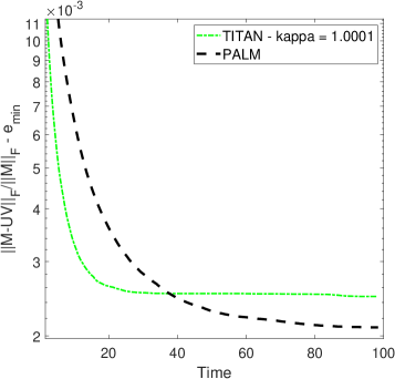
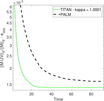
Umist	ORL

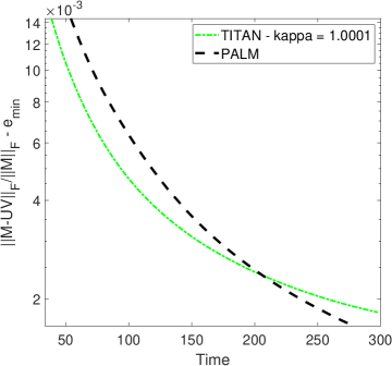
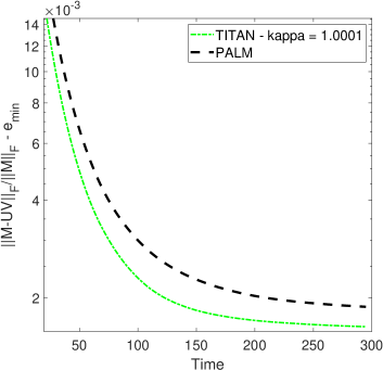
Figure 1: TITAN and PALM applied on sparse NMF. The plots show the evolution of the average value of $E(k)$ with respect to time on the image data sets.

Table 1: Average and std of relative errors obtained by TITAN and PALM applied on sparse NMF (3). Bold values correspond to the best results for each data set.

Data set	Method	mean $\pm$ std
Frey	PALM	$\mathbf{1.4901\,10^{-1}\pm 1.0342\,10^{-3}}$
	TITAN - $\kappa=1.0001$	$1.4939\,10^{-1}\pm 1.0448\,10^{-3}$
cbclim	PALM	$1.1955\,10^{-1}\pm 7.4322\,10^{-4}$
	TITAN - $\kappa=1.0001$	$\mathbf{1.1939\,10^{-1}\pm 7.1868\,10^{-4}}$
Umist	PALM	$\mathbf{1.2002\ 10^{-1}\pm 8.1340\,10^{-4}}$
	TITAN - $\kappa=1.0001$	$1.2031\,10^{-1}\pm 9.3527\,10^{-4}$
ORL	PALM	$1.9108\,10^{-1}\pm 6.5507\,10^{-4}$
	TITAN - $\kappa=1.0001$	$\mathbf{1.9084\,10^{-1}\pm 8.4325\,10^{-4}}$

We observe that TITAN - $\kappa=1.0001$ converges initially faster than PALM for all data sets. In term of the accuracy of the final solutions, TITAN - $\kappa=1.0001$ provides better relative errors on average for the CBCL and ORL data sets, while PALM for the Frey and Umist data sets. This is expected since sparse NMF is a hard nonconvex problem, and hence different algorithms converge towards different critical points with different objective function values (even if they are initialized with the same solution).

Sparse document data sets

In the second experiment, we test the two algorithms on six sparse document data sets: classic, sports, reviews, hitech, k1b and tr11, see Zhong and Ghosh (2005). We choose $\mathbf{r}=25$, $s=0.25\mathbf{r}$, run all algorithms 20 times, use the same random initialization for all algorithms in each run, and run each algorithm for 100 seconds. Figure 2 reports the evolution with respect to time of the average values of $E(k)$. Table 2 reports the average and the standard deviation (std) of the relative errors.

classic	sports
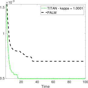
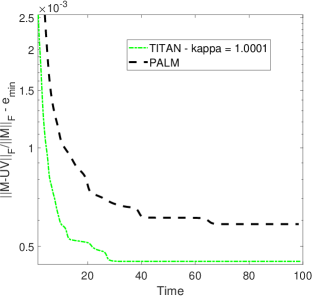
reviews	hitech
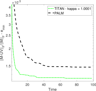
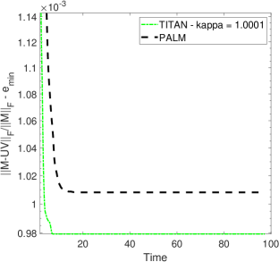
k1b	tr11

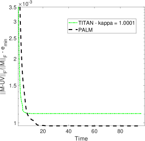
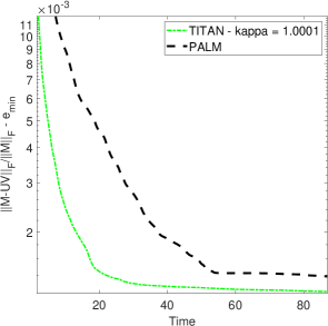
Figure 2: TITAN and PALM applied on sparse NMF. The plots show the evolution of the average value of $E(k)$ with respect to time on the sparse document data sets.

Table 2: Average and std of relative errors obtained by TITAN and PALM applied on sparse NMF (3). Bold values correspond to the best results for each data set.

Data set	Method	mean $\pm$ std
classic	PALM	$8.9160\,10^{-1}\pm 7.4522\,10^{-4}$
	TITAN - $\kappa=1.0001$	$\mathbf{8.9145\,10^{-1}\pm 3.1633\,10^{-4}}$
sports	PALM	$8.1190\,10^{-1}\pm 4.3938\,10^{-4}$
	TITAN - $\kappa=1.0001$	$\mathbf{8.1177\,10^{-1}\pm 2.9569\,10^{-4}}$
reviews	PALM	$8.0803\ 10^{-1}\pm 5.6695\,10^{-4}$
	TITAN - $\kappa=1.0001$	$\mathbf{8.0779\,10^{-1}\pm 7.0906\,10^{-4}}$
hitech	PALM	$8.6305\,10^{-1}\pm 5.5024\,10^{-4}$
	TITAN - $\kappa=1.0001$	$\mathbf{8.6302\,10^{-1}\pm 6.2594\,10^{-4}}$
k1b	PALM	$\mathbf{8.1829\ 10^{-1}\pm 6.1890\,10^{-4}}$
	TITAN - $\kappa=1.0001$	$8.1842\,10^{-1}\pm 7.5261\,10^{-4}$
tr11	PALM	$1.4768\ 10^{-1}\pm 7.4810\,10^{-4}$
	TITAN - $\kappa=1.0001$	$\mathbf{1.4752\,10^{-1}\pm 5.3136\,10^{-4}}$

We again observe that TITAN - $\kappa=1.0001$ converges on average faster than PALM in all data sets. In terms of the relative errors of the final solutions computed within the allotted time, TITAN - $\kappa=1.0001$ performs on average better than PALM, except for the k1b data set.

6.2 Matrix Completion Problem

In this section, we illustrate the advantages of using block surrogate functions by deploying TITAN for the MCP (4), as explained in Section 4.5. As for sparse NMF, we use two blocks of variables, $x_{1}=U$ and $x_{2}=V$. Since $\psi(U,V)$ is continuously differentiable and $\mathcal{R}(U,V)$ is a block separable function, $F$ (in this case $F=f$) satisfies the condition in (1). Moreover, $\phi$ is block-wise concave and differentiable with Lipschitz gradient on $\mathbb{R}^{\mathbf{m}\times\mathbf{n}}_{+}$. Hence, we select the composite surrogate function for $f=\psi+\phi\circ r$ as in Section 4.5, in which we will choose block surrogate functions for $\psi$ as follows. Since $\nabla_{U}\psi(U,V)=-\mathcal{P}(A-UV)V^{T}$ and $\nabla_{V}\psi(U,V)=-U^{T}\mathcal{P}(A-UV)$ are Lipschitz continuous with constants $L_{1}=\|VV^{T}\|$ and $L_{2}=\|U^{T}U\|$, respectively, we choose the block surrogate functions $u_{i}^{\psi}$, $i=1,2$, for $\psi$ to be the block Lipschitz gradient surrogate functions as in Section 4.2. Assumption 2 is then satisfied; see Section 4.5.

Let us choose the Nesterov-type acceleration. The update in (6) for $U$ is

$$\begin{split}U^{k+1}\in\operatorname*{argmin}_{U}\left\langle{\nabla_{U}\psi(\bar{U}^{k},V^{k})},{U}\right\rangle+\frac{L_{1}^{k}}{2}\|U-\bar{U}^{k}\|^{2}+\langle\nabla_{U}\phi(r(U^{k},V^{k})),|U|\rangle,\end{split}$$ (38)

where $\nabla_{U}\phi(r(U^{k},V^{k}))=\lambda\theta\left(\exp(-\theta\|u_{ij}^{k}\|)\right)$, $L_{1}^{k}=\|V^{k}(V^{k})^{T}\|$, $\bar{U}^{k}=U^{k}+\beta_{1}^{k}(U^{k}-U^{k-1})$. The solution of (38) is given by

$$U^{k+1}=\mathcal{S}_{1/L_{1}^{k}}\left(P^{k},\nabla_{U}\phi\left(r\left(U^{k},V^{k}\right)\right)\right),$$ (39)

where $P^{k}=\bar{U}^{k}-\frac{1}{L_{1}^{k}}\nabla_{U}\psi(\bar{U}^{k},V^{k})$, and $\mathcal{S}_{\tau}$ is the soft-thresholding operator with parameter $\tau$, that is,

$$\mathcal{S}_{\tau}(P,W)_{ij}=[|p_{ij}|-\tau w_{ij}]_{+}\text{sign}(p_{ij}).$$ (40)

Similarly ,the update for $V$ is given by

$$V^{k+1}=\mathcal{S}_{1/L_{2}^{k}}\left(Q^{k},\nabla_{V}\phi\left(r\left(U^{k+1},V^{k}\right)\right)\right),$$ (41)

where $L_{2}^{k}=\|(U^{k+1})^{T}U^{k+1}\|$, $Q^{k}=\bar{V}^{k}-\frac{1}{L_{2}^{k}}\nabla_{V}\psi(U^{k+1},\bar{V}^{k})$ and $\bar{V}^{k}=V^{k}+\beta^{k}_{2}(V^{k}-V^{k-1})$.

Let us now determine $\eta_{i}^{k}$ and $\gamma_{i}^{k}$, for $i=1,2$, of Condition (14). Note that $x_{i}\mapsto\langle\nabla_{i}\phi(r(y)),r_{i}(x_{i})\rangle$ are convex. Furthermore, $\psi(U,V)$ is a block-wise convex function. Therefore, it follows from Remark 12 that we can take $\eta_{i}^{k}$ and $\gamma_{i}^{k}$ as in (24). Note that $\tau_{i}^{k}=\beta_{i}^{k}$, since we choose Nesterov-type acceleration. Condition (14) becomes $\beta_{i}^{k}\leq\sqrt{{CL_{i}^{k-1}}/{L_{i}^{k}}},$ where $0<C<1$. In our experiments, we choose

$$\begin{array}[]{ll}C=0.9999^{2},\mu_{0}=1,\mu_{k}=\frac{1}{2}(1+\sqrt{1+4\mu_{k-1}^{2}}),\\ \beta_{i}^{k}=\min\Big{\{}\frac{\mu_{k}-1}{\mu_{k}},\sqrt{{CL_{i}^{k-1}}/{L_{i}^{k}}}\Big{\}}.\end{array}$$ (42)

We compare three algorithms: (1) TITAN without extrapolation, that is, $\beta_{i}^{k}=0$ for all $k$, which is denoted by TITAN-NO, (2) TITAN with extrapolation, that is, $\beta_{i}^{k}$ are chosen as in (42), which is denoted by TITAN-EXTRA, and (3) PALM that alternatively updates $U$ and $V$ by solving the following sub-problems

$$\begin{array}[]{ll}\min\limits_{U}\left\langle{\nabla_{U}\psi(U^{k},V^{k})},{U}\right\rangle+\frac{L_{1}(V^{k})}{2}\|U-U^{k}\|^{2}+\lambda\sum_{ij}\Big{(}1-\exp(-\theta|u_{ij}|)\Big{)},\\ \min\limits_{V}\left\langle{\nabla_{V}\psi(U^{k+1},V^{k})},{V}\right\rangle+\frac{L_{2}(U^{k+1})}{2}\|V-V^{k}\|^{2}+\lambda\sum_{ij}\Big{(}1-\exp(-\theta|v_{ij}|)\Big{)}.\end{array}$$

These sub-problems can be separated into one-dimensional nonconvex problems

$$\min_{x\in\mathbb{R}}\frac{1}{2}\|x-v\|^{2}-\gamma\exp(-\theta|x|).$$ (43)

Although the solutions to these subproblems can be computed via the Lambert $W$ function (Corless et al., 1996), it does not have a closed-form solution. To the best of our knowledge, TITAN is the only framework that allows to use extrapolation while having closed-form updates to solve this particular matrix completion formulation.

In our experiments, all the algorithms start from the same initial point $(U^{0},V^{0})$, where $U^{0}$ is an $\mathbf{m}\times\mathbf{r}$ orthogonal matrix whose range approximates the range of $\mathcal{P}(A)$, which is computed by a power method (Halko et al., 2011, Algorithm 4.1) with $\mathbf{r}$ iterations and a tolerance $10^{-6}$. The initial matrix $V^{0}$ is determined by $V^{0}=\mathbf{V}^{T}$ with $U\Sigma V^{T}$ being the singular value decomposition of $(U^{0})^{T}\mathcal{P}(A)$, i.e., $U\Sigma V^{T}=(U^{0})^{T}\mathcal{P}(A)$. We choose $\lambda=0.1$ and $\theta=5$. We note that we do not optimize numerical results by tweaking the parameters as this is beyond the scope of this work. Rather, we simply chose the parameters that are typically used in the literature, see, e.g., Bradley and Mangasarian (1998). It is important noting that we evaluate the algorithms on the same models. We carried out the experiments on the two most widely used data sets in the field of recommendation systems, MovieLens and Netflix, which contain ratings of different users. The characteristics of the data sets are given in Table 3. We respectively choose $\mathbf{r}=5,8$, and $13$ for MovieLens 1M, 10M, and Netflix data set. We randomly picked 70% of the observed ratings for training and the rest for testing. The process was repeated twenty times. We run each algorithm 20, 200, and 3600 seconds for MovieLens 1M, 10M, and Netflix data sets, respectively. We are interested in the root mean squared error on the test set: $RMSE=\sqrt{\|\mathcal{P}_{T}(A-UV)\|^{2}/N_{T}}$, where $\mathcal{P}_{T}(Z)_{ij}=Z_{ij}$ if $A_{ij}$ belongs to the test set and $0$ otherwise, $N_{T}$ is the number of ratings in the test set. We plotted the curves of the average value of RMSE and the objective function value versus training time in Figure 3, and report the average and the standard deviation of the RMSE and the objective function value in Table 4.

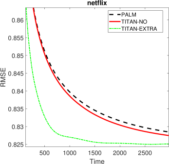
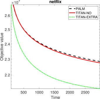
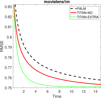
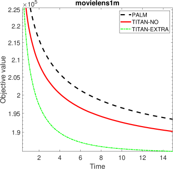
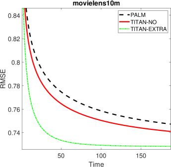
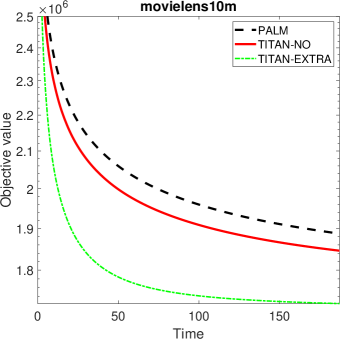
Figure 3: TITAN and PALM applied on the MCP (4). Evolution of the average value of the RMSE on the test set and the objective function value with respect to time.

Table 3: The number of users, items, and ratings used in each data set.

Data set		#users	#items	#ratings
MovieLens	1M	6,040	3,449	999,714
	10M	69,878	10,677	10,000,054
Netflix		480,189	17,770	100,480,507

Table 4: Comparison of TITAN and PALM applied on the MCP (4): RMSE and final objective function values obtained within the allotted time. Bold values indicate the best results for each data set.

Data set	Method	RMSE	Objective value
		mean $\pm$ std	(mean $\pm$ std)$\times 10^{-5}$
MovieLens 1M	PALM	0.7550 $\pm$ 0.0016	1.9155 $\pm$ 0.0088
	TITAN-NO	0.7514 $\pm$ 0.0013	1.8879 $\pm$ 0.0066
	TITAN-EXTRA	0.7509 $\pm$ 0.0008	1.8483 $\pm$ 0.0038
MovieLens 10M	PALM	0.7462 $\pm$ 0.0006	18.8038 $\pm$ 0.0348
	TITAN-NO	0.7402 $\pm$ 0.0006	18.4027 $\pm$ 0.0375
	TITAN-EXTRA	0.7283 $\pm$ 0.0005	17.2277 $\pm$ 0.0236
Netflix	PALM	0.8274 $\pm$ 0.0006	226.4846 $\pm$ 1.1898
	TITAN-NO	0.8265 $\pm$ 0.0006	225.4806 $\pm$ 1.1808
	TITAN-EXTRA	0.8250 $\pm$ 0.0004	210.4999 $\pm$ 0.3569

We observe that TITAN-EXTRA converges the fastest on all the data sets, providing a significant acceleration of TITAN-NO: as shown on Table 5, TITAN-EXTRA is at least 4 times faster than TITAN-NO on the three data sets. TITAN-EXTRA achieves not only the best final objective function values but also the best RMSE on the test set. This illustrates the usefulness of the inertial terms. Moreover, TITAN-NO performs better PALM on the three data sets which illustrates the usefulness of properly choosing the surrogate function. Recall that TITAN-NO and TITAN-EXTRA are two new algorithms for the MCP (4), which are specific instances of the TITAN framework.

data set	TITAN-EXTRA	TITAN-NO	acceleration
	lead time (s)	total time (s)	factor
netflix	674.91	3000	4.44
movielens1m	3.8	15	3.94
movielens10m	28.67	200	6.97

Table 5: TITAN lead time compared to TITAN-NO to obtain the same objective function value within the allotted time.

7 Conclusion

We have proposed and analysed TITAN, a novel inertial block majorization-minimization algorithmic framework. TITAN unifies many inertial block coordinate descent methods, while allowing to derive new highly efficient algorithms, as illustrated in Section 6.2 on the MCP. We proved sub-sequential convergence of TITAN under mild assumptions and global convergence of TITAN under some stronger assumptions. We applied TITAN to sparse NMF and the MCP to illustrate the benefit of using inertial terms in BCD methods, and of using proper surrogate functions. Especially, the way we choose the surrogate functions and the corresponding extrapolation operators to derive TITAN-based algorithms for the MCP illustrated the advantages of using TITAN compared to the typical proximal BCD methods. Our future research direction include the development of TITAN-based algorithms for solving specific practical problems, for which using typical proximal BCD methods is not efficient (in particular when a closed-form for the subproblems in each block of variables does not exist).

A Preliminaries of nonconvex nonsmooth optimization

Let $g:\mathbb{E}\to\mathbb{R}\cup\{+\infty\}$ be a proper lower semicontinuous function.

Definition 14

• For each $x\in{\rm dom}\,g,$ we denote $\hat{\partial}g(x)$ as the Frechet subdifferential of $g$ at $x$ which contains vectors $v\in\mathbb{E}$ satisfying

  $$\liminf_{y\neq x,y\to x}\frac{1}{\left\|y-x\right\|}\left(g(y)-g(x)-\left\langle v,y-x\right\rangle\right)\geq 0.$$

  If $x\not\in{\rm dom}\>g,$ then we set $\hat{\partial}g(x)=\emptyset.$

• The limiting-subdifferential $\partial g(x)$ of $g$ at $x\in{\rm dom}\>g$ is defined as follows.

  $$\partial g(x):=\left\{v\in\mathbb{E}:\exists x^{k}\to x,\,g\big{(}x^{k}\big{)}\to g(x),\,v^{k}\in\hat{\partial}g\big{(}x^{k}\big{)},\,v^{k}\to v\right\}.$$

Definition 15

We call $x^{*}\in\rm{dom}\,F$ a critical point of $F$ if $0\in\partial F\left(x^{*}\right).$

We note that if $x^{*}$ is a local minimizer of $F$ then $x^{*}$ is a critical point of $F$.

Definition 16

A function $\phi(x)$ is said to have the KL property at $\bar{x}\in{\rm dom}\,\partial\,\phi$ if there exists $\eta\in(0,+\infty]$, a neighborhood $U$ of $\bar{x}$ and a concave function $\xi:[0,\eta)\to\mathbb{R}_{+}$ that is continuously differentiable on $(0,\eta)$, continuous at $0$, $\xi(0)=0$, and $\xi^{\prime}(s)>0$ for all $s\in(0,\eta),$ such that for all $x\in U\cap[\phi(\bar{x})<\phi(x)<\phi(\bar{x})+\eta],$ we have

$$\xi^{\prime}\left(\phi(x)-\phi(\bar{x})\right)\,\operatorname*{dist}\left(0,\partial\phi(x)\right)\geq 1.$$ (44)

$\operatorname*{dist}\left(0,\partial\phi(x)\right)=\min\left\{\|y\|:y\in\partial\phi(x)\right\}$. If $\phi(x)$ has the KL property at each point of ${\rm dom}\,\partial\phi$ then $\phi$ is a KL function.

Many nonconvex nonsmooth functions in practical applications belong to the class of KL functions, for examples, real analytic functions, semi-algebraic functions, and locally strongly convex functions, see Bochnak et al. (1998); Bolte et al. (2014).

B Global convergence recipe

Let us recall Theorem 2 of Hien et al. (2020).

Theorem 17

(Hien et al., 2020, Theorem 2) Let $\Phi:\mathbb{R}^{N}\to(-\infty,+\infty]$ be a proper and lower semicontinuous function which is bounded from below. Let $\mathcal{A}$ be a generic algorithm which generates a bounded sequence $\left\{z^{k}\right\}$ by $z^{0}\in\mathbb{R}^{N}$, $z^{k+1}\in\mathcal{A}(z^{k})$, $k=0,1,\ldots$ Assume that there exist positive constants $\rho_{1},\rho_{2}$ and $\rho_{3}$ and a non-negative sequence $\left\{\varphi_{k}\right\}_{k\in\mathbb{N}}$ such that the following conditions are satisfied:

• Sufficient decrease property:

  $$\rho_{1}\|z^{k}-z^{k+1}\|^{2}\leq\rho_{2}\varphi_{k}^{2}\leq\Phi(z^{k})-\Phi(z^{k+1}),k=0,1,\ldots$$

• Boundedness of subgradient:

  $$\|\omega^{k+1}\|\leq\rho_{3}\varphi_{k},\omega^{k}\in\partial\Phi(z^{k})\;\text{ for }\;k=0,1,\ldots$$

• KL property: $\Phi$ is a KL function.

• A continuity condition: If a subsequence $\{z^{k_{n}}\}$ converges to $\bar{z}$ then $\Phi(z^{k_{n}})$ converges to $\Phi(\bar{z})$ as $n$ goes to $\infty$.

Then we have $\sum_{k=1}^{\infty}\varphi_{k}<\infty$, and $\{z^{k}\}$ converges to a critical point of $\Phi$.

C Technical proofs

In this section, we provide the proofs for Theorem 8 and Proposition 13.

C.1 Proof of Theorem 8

Let $x^{*}$ be a limit point of $x^{k}$. From Theorem 6 we have $x^{*}$ is a critical point of $\Phi$. As the generated sequence $\{x^{k}\}$ is assumed to be bounded, in the following, we only work on the bounded set that contains $\{x^{k}\}$.

Case 1: $C<\underline{l}/\overline{l}$. Define $\Phi^{\delta}(x,y):=\Phi(x)+\sum_{i=1}^{m}\frac{\delta_{i}}{2}\|x_{i}-y_{i}\|^{2}.$ Let $z^{k}=(x^{k},x^{k-1})$ and $\varphi_{k}^{2}=\frac{1}{2}\|x^{k+1}-x^{k}\|^{2}+\frac{1}{2}\|x^{k}-x^{k-1}\|^{2}$ . We verify the conditions of Theorem 17 for $\Phi^{\delta}(x^{k},x^{k-1})$ with $\delta_{i}=(\underline{l}+C\overline{l})/2$.

(B1) Sufficient decrease property. From Inequality (17), we have

$$F(x^{k+1})+\underline{l}\|x^{k+1}-x^{k}\|^{2}\leq F(x^{k})+C\overline{l}\|x^{k}-x^{k-1}\|^{2}.$$

Hence, $\Phi^{\delta}(z^{k})-\Phi^{\delta}(z^{k+1})\geq(\underline{l}-C\overline{l})\varphi_{k}^{2}$.

(B2) Boundedness of subgradient. We note that

$$\partial_{x}\Phi^{\delta}(x,y)=\partial\Phi(x)+[\delta_{i}(x_{i}-y_{i})|_{i=1,\ldots,m}],\quad\partial_{y}\Phi^{\delta}(x,y)=[\delta_{i}(y_{i}-x_{i})|_{i=1,\ldots,m}].$$ (45)

Writing the optimality condition for (6), we have

$$\mathcal{G}^{k}_{i}(x^{k}_{i},x^{k-1}_{i})\in\partial_{x_{i}}\big{(}u_{i}(x_{i}^{k+1},x^{k,i-1})+\mathcal{I}_{\mathcal{X}_{i}}(x_{i}^{k+1})+g_{i}(x_{i}^{k+1})\big{)}.$$

Hence, by Assumption 3 (i), there exist $\mathbf{s}_{i}^{k}\in\partial_{x_{i}}u_{i}(x_{i}^{k+1},x^{k,i-1})$ and $\mathbf{v}_{i}^{k}\in\mathcal{\partial}(I_{\mathcal{X}_{i}}(x_{i}^{k+1})+g_{i}(x_{i}^{k+1}))$ such that

$$\mathcal{G}^{k}_{i}(x^{k}_{i},x^{k-1}_{i})=\mathbf{s}^{k}_{i}+\mathbf{v}_{i}^{k}.$$

As we assume Assumption 3 (ii) holds, there exists $\mathbf{t}_{i}^{k}\in\partial_{x_{i}}f(x^{k+1})$ such that

$$\|\mathbf{s}_{i}^{k}-\mathbf{t}_{i}^{k}\|\leq B_{i}\|x^{k+1}-x^{k,i-1}\|.$$

We note that $\mathbf{t}_{i}^{k}+\mathbf{v}_{i}^{k}\in\partial_{x_{i}}\Phi(x^{k+1})$ by Assumption 3 (i). On the other hand,

$$\|\mathbf{t}_{i}^{k}+\mathbf{v}_{i}^{k}\|=\|\mathbf{t}_{i}^{k}-\mathbf{s}_{i}^{k}+\mathbf{s}_{i}^{k}+\mathbf{v}_{i}^{k}\|\leq B_{i}\|x^{k+1}-x^{k,i-1}\|+A^{k}_{i}\|x^{k}_{i}-x^{k-1}_{i}\|,$$

which implies the boundedness of the subgradient since $A^{k}_{i}$ is bounded.

(B3) KL property. As $\Phi$ is a KL function, $\Phi^{\delta}$ is also a KL function.

(B4) A continuity condition. Suppose $z^{k_{n}}\to z^{*}$. From Proposition 5, we have that if $x^{k_{n}}$ converges to $x^{*}$ then $x^{k_{n}-1}$ also converges to $x^{*}$. Hence $z^{*}=(x^{*},x^{*})$. On the other hand, we can derive from (10) that, for $i\in[m]$, $u_{i}(x_{i}^{k_{n}},x^{k_{n}-1,i-1})+g_{i}(x_{i}^{k_{n}})$ converges to $u_{i}(x_{i}^{*},x^{*})+g_{i}(x_{i}^{*})$. As we assume $u_{i}(\cdot,\cdot)$ is continuous we have $u_{i}(x_{i}^{k_{n}},x^{k_{n}-1,i-1})$ converges to $u_{i}(x_{i}^{*},x^{*})=f(x^{*})$. Hence, $g_{i}(x_{i}^{k_{n}})\to g_{i}(x_{i}^{*})$. We then have $F(x^{k_{n}})=f(x^{k_{n}})+\sum g_{i}(x^{k_{n}}_{i})$ converges to $F(x^{*})$, which leads to $\Phi^{\delta}(z^{k_{n}+1})$ converges to $\Phi^{\delta}(z^{*})$

Applying Theorem 17, we get $0\in\partial\Phi^{\delta}(x^{*},x^{*})$, which leads to $0\in\partial\Phi(x^{*})$.

Case 2: With restart. We use the technique in the proof of (Bolte et al., 2014, Theorem 1) with some modification. A restarting step would be taken when $F(x^{k+1})\geq F(x^{k})$. When restarting happens, Condition (NSDP) is assumed to be satisfied with $\gamma_{i}^{k}=0$, we thus have

$$F(x^{k+1})+\sum_{i=1}^{m}\frac{\eta_{i}^{k}}{2}\|x_{i}^{k+1}-x_{i}^{k}\|^{2}\leq F(x^{k}).$$ (46)

Hence, we have

$$F(x^{k+1})+\sum_{i=1}^{m}\frac{\eta_{i}^{k}}{2}\|x_{i}^{k+1}-x_{i}^{k}\|^{2}\leq F(x^{k})+\hat{C}\sum_{i=1}^{m}\frac{\eta_{i}^{k-1}}{2}\|x_{i}^{k}-x_{i}^{k-1}\|^{2},$$ (47)

where $\hat{C}=C$ in normal situation as in Inequality (17) and $\hat{C}=0$ when restarting happens. Thus the result in Proposition 5 does not change. Exactly as for the proof of the continuity condition (B4) above (the first case), we can show that $F(x^{k_{n}})\to F(x^{*})$. Since $F(x^{k})$ is non-increasing we have $F(x^{k})\to F(x^{*})$. This also means $\Phi(x)$ is constant on the set $\Omega$ of all limit points of $x^{k}$. From Proposition 5, we have $\|x^{k}-x^{k-1}\|\to 0$. Hence, (Bolte et al., 2014, Lemma 5) yields that $\Omega$ is a compact and connected set.

Let us recall that restarting happens when $F(x^{k+1})\geq F(x^{k})$ and when it happens Inequality (46) holds. Therefore, as long as $x^{k+1}\neq x^{k}$, $F(x^{k})$ is strictly decreasing (that is $F(x^{k+1})<F(x^{k})$). Hence, if there exists an integer $\bar{k}$ such that $F(x^{\bar{k}})=F(x^{*})$ then we have $F(x^{k})=F(x^{*})$ and $x^{k}=x^{\bar{k}}$ for all $k\geq\bar{k}$. So this case is trivial.

Let us consider $F(x^{k})>F(x^{*})$ for all $k$. Then there exists a positive integer $k_{0}$ such that $F(x^{k})<F(x^{*})+\eta$ for all $k>k_{0}$. On the other hand, there exists a positive integer $k_{1}$ such that ${\rm dist}(x^{k},\Omega)<\varepsilon$ for all $k>k_{1}$. Applying (Bolte et al., 2014, Lemma 6) we have

$$\xi^{\prime}\big{(}\Phi\left(x^{k}\right)-\Phi(x^{*})\big{)}\operatorname*{dist}\big{(}0,\partial\Phi(x^{k})\big{)}\geq 1,\text{for any}\,k>\mathbf{k}:=\max\{k_{0},k_{1}\}.$$ (48)

On the other hand, exactly as for Case 1 without restarting step, we can prove that $\exists\varpi>0$ such that for some $\omega^{k+1}\in\partial\Phi(x^{k+1})$ we have $\|\omega^{k+1}\|\leq\varpi\varphi_{k}\leq\frac{\varpi}{\sqrt{2}}(\|x^{k+1}-x^{k}\|+\|x^{k}-x^{k-1}\|).$ Therefore, it follows from (48) that

$$\begin{array}[]{ll}\xi^{\prime}\big{(}\Phi\left(x^{k}\right)-\Phi(x^{*})\big{)}(\|x^{k+1}-x^{k}\|+\|x^{k}-x^{k-1}\|)\geq\frac{\sqrt{2}}{\varpi}\end{array}$$ (49)

From Inequality (47) and noting that $\bar{C}\leq C$, we get

$$\begin{array}[]{ll}\Phi(x^{k})-\Phi(x^{k+1})\geq\sum_{i=1}^{m}\frac{\eta_{i}^{k}}{2}\|x_{i}^{k+1}-x_{i}^{k}\|^{2}-C\sum_{i=1}^{m}\frac{\eta_{i}^{k-1}}{2}\|x_{i}^{k}-x_{i}^{k-1}\|^{2}\end{array}$$ (50)

Denote $A_{i,j}=\xi(\Phi(x^{i})-\Phi(x^{*}))-\xi(\Phi(x^{j})-\Phi(x^{*}))$. From the concavity of $\xi$ we get $A_{k,k+1}\geq\xi^{\prime}\big{(}\Phi\left(x^{k}\right)-\Phi(x^{*})\big{)}\big{(}\Phi(x^{k})-\Phi(x^{k+1})\big{)}$. Together with (49) and (50) we get

$$\sum_{i=1}^{m}\frac{\eta_{i}^{k}}{2}\|x_{i}^{k+1}-x_{i}^{k}\|^{2}\leq C\sum_{i=1}^{m}\frac{\eta_{i}^{k-1}}{2}\|x_{i}^{k}-x_{i}^{k-1}\|^{2}+\frac{\varpi}{\sqrt{2}}A_{k,k+1}(\|x^{k+1}-x^{k}\|+\|x^{k}-x^{k-1}\|)$$ (51)

Denote $\Upsilon^{k}=\sum_{i=1}^{m}\frac{\eta_{i}^{k}}{2}\|x_{i}^{k+1}-x_{i}^{k}\|^{2}$. Using inequality $\sqrt{a+b}\leq\sqrt{a}+\sqrt{b}$ and $\sqrt{ab}\leq ta+b/4t$, for $t>0$, from (51) we get

$$\begin{array}[]{ll}\sqrt{\Upsilon^{k}}&\leq\sqrt{C\Upsilon^{k-1}}+\sqrt{\frac{\varpi A_{k,k+1}}{\sqrt{2}}(\|x^{k+1}-x^{k}\|+\|x^{k}-x^{k-1}\|)}\\ &\leq\sqrt{C\Upsilon^{k-1}}+\frac{(1-\sqrt{C})\sqrt{\underline{l}}}{3}(\|x^{k+1}-x^{k}\|+\|x^{k}-x^{k-1}\|)+\frac{3\varpi A_{k,k+1}}{4\sqrt{2}\sqrt{\underline{l}}(1-\sqrt{C})}\end{array}$$

Summing up this inequality from $k=\mathbf{k}+1$ to $K$ we obtain

$$\sqrt{\Upsilon^{K}}+\sum_{k=\mathbf{k}+1}^{K-1}(1-\sqrt{C})\sqrt{\Upsilon^{k}} \leq\sqrt{C\Upsilon^{\mathbf{k}}}+\frac{(1-\sqrt{C})\sqrt{\underline{l}}}{3}\sum_{k=\mathbf{k}+1}^{K}(\|x^{k+1}-x^{k}\|+\|x^{k}-x^{k-1}\|)$$

$$\qquad\qquad+\frac{3\varpi}{4\sqrt{2}\sqrt{\underline{l}}(1-\sqrt{C})}A_{\mathbf{k}+1,K+1}.$$

On the other hand, we note that $\sqrt{\Upsilon^{k}}\geq\sqrt{\underline{l}}\|x^{k+1}-x^{k}\|$. Therefore, we get

$$\frac{2}{3}(1-\sqrt{C})\sqrt{\underline{l}}\sum_{k=\mathbf{k}+1}^{K}\|x^{k+1}-x^{k}\|\leq\frac{(1-\sqrt{C})\sqrt{\underline{l}}}{3}\sum_{k=\mathbf{k}+1}^{K}\|x^{k}-x^{k-1}\|+\frac{3\varpi A_{\mathbf{k}+1,K+1}}{4\sqrt{2}\sqrt{\underline{l}}(1-\sqrt{C})},$$

which implies that $\sum_{k=\mathbf{k}+1}^{K}\|x^{k+1}-x^{k}\|\leq\|x^{\mathbf{k}+1}-x^{\mathbf{k}}\|+\frac{9\varpi}{4\sqrt{2}(1-\sqrt{C})^{2}\underline{l}}A_{\mathbf{k},K+1}.$ Hence, $\sum_{k=1}^{\infty}\|x^{k+1}-x^{k}\|<+\infty$. The result follows.

C.2 Proof of Proposition 13

Let us prove Statement (A). Statement (B) of Proposition 13 is a consequence of Statement (A). From Inequality (35) we get

$$F(\mathbf{x}^{k,j})+\frac{\bar{\eta}^{k,l-1}_{i}}{2}\|\bar{\mathbf{x}}^{k,l}_{i}-\bar{\mathbf{x}}^{k,l-1}_{i}\|^{2}\leq F(\mathbf{x}^{k,j-1})+\frac{C\bar{\eta}^{k,l-2}_{i}}{2}\|\bar{\mathbf{x}}^{k,l-1}_{i}-\bar{\mathbf{x}}^{k,l-2}_{i}\|^{2}.$$ (52)

Summing up Inequality (52) from $j=1$ to $T$ we obtain

$$F(\mathbf{x}^{k+1})+\sum_{i=1}^{m}\sum_{l=1}^{d_{i}^{k}}\frac{\bar{\eta}^{k,l-1}_{i}}{2}\|\bar{\mathbf{x}}^{k,l}_{i}-\bar{\mathbf{x}}^{k,l-1}_{i}\|^{2}\leq F(\mathbf{x}^{k})+C\sum_{i=1}^{m}\sum_{l=1}^{d_{i}^{k}}\frac{\bar{\eta}^{k,l-2}_{i}}{2}\|\bar{\mathbf{x}}^{k,l-1}_{i}-\bar{\mathbf{x}}^{k,l-2}_{i}\|^{2}.$$

Therefore,

$$\begin{split}&F(\mathbf{x}^{k+1})+C\sum_{i=1}^{m}\frac{\bar{\eta}_{i}^{k,d^{k}_{i}-1}}{2}\|\bar{\mathbf{x}}^{k,d^{k}_{i}}_{i}-\bar{\mathbf{x}}^{k,d^{k}_{i}-1}_{i}\|^{2}+(1-C)\sum_{i=1}^{m}\sum_{l=1}^{d_{i}^{k}}\frac{\bar{\eta}_{i}^{k,l-1}}{2}\|\bar{\mathbf{x}}^{k,l}_{i}-\bar{\mathbf{x}}^{k,l-1}_{i}\|^{2}\\ &\qquad\leq F(\mathbf{x}^{k})+C\sum_{i=1}^{m}\frac{\bar{\eta}_{i}^{k,-1}}{2}\|\bar{\mathbf{x}}^{k,0}_{i}-\bar{\mathbf{x}}^{k,-1}_{i}\|^{2}.\end{split}$$ (53)

Note that $\bar{\mathbf{x}}^{k,0}_{i}=\bar{\mathbf{x}}^{k-1,d_{i}^{k-1}}_{i}$, $\bar{\mathbf{x}}^{k,-1}_{i}=\bar{\mathbf{x}}^{k-1,d_{i}^{k-1}-1}_{i}=(\mathbf{x}^{k-1}_{prev})_{i}$ and $\bar{\eta}_{i}^{k+1,-1}=\bar{\eta}_{i}^{k,d_{i}^{k}}$. Hence, from (53) we obtain

$$\begin{split}&F(\mathbf{x}^{k+1})+C\sum_{i=1}^{m}\frac{\bar{\eta}_{i}^{k+1,-1}}{2}\|\mathbf{x}^{k+1}_{i}-(\mathbf{x}^{k+1}_{prev})_{i}\|^{2}+(1-C)\sum_{i=1}^{m}\sum_{l=1}^{d_{i}^{k}}\frac{\bar{\eta}_{i}^{k,l-1}}{2}\|\bar{\mathbf{x}}^{k,l}_{i}-\bar{\mathbf{x}}^{k,l-1}_{i}\|^{2}\\ &\qquad\leq F(\mathbf{x}^{k})+C\sum_{i=1}^{m}\bar{\eta}_{i}^{k,-1}\|\mathbf{x}^{k}_{i}-(\mathbf{x}^{k}_{prev})_{i}\|^{2}.\end{split}$$ (54)

Summing up Inequality (54) from $k=0$ to $K-1$ we get

$$\begin{array}[]{ll}&F(\mathbf{x}^{K})+C\sum\limits_{i=1}^{m}\frac{\bar{\eta}_{i}^{K,-1}}{2}\|\mathbf{x}^{K}_{i}-(\mathbf{x}^{K}_{prev})_{i}\|^{2}+(1-C)\sum_{k=0}^{K-1}\sum\limits_{i=1}^{m}\sum\limits_{l=1}^{d_{i}^{k}}\frac{\bar{\eta}_{i}^{k,l-1}}{2}\|\bar{\mathbf{x}}^{k,l}_{i}-\bar{\mathbf{x}}^{k,l-1}_{i}\|^{2}\\ &\qquad\leq F(\mathbf{x}^{0})+C\sum\limits_{i=1}^{m}\frac{\bar{\eta}_{i}^{0,-1}}{2}\|\mathbf{x}^{0}_{i}-(\mathbf{x}^{0}_{prev})_{i}\|^{2},\end{array}$$

which gives the result.

References

- Adly and Attouch (2020) S. Adly and H. Attouch. Finite convergence of proximal-gradient inertial algorithms combining dry friction with Hessian-driven damping. SIAM Journal on Optimization, 30(3):2134–2162, 2020. doi: 10.1137/19M1307779. URL https://doi.org/10.1137/19M1307779.
- Aharon et al. (2006) M. Aharon, M. Elad, A. Bruckstein, et al. K-svd: An algorithm for designing overcomplete dictionaries for sparse representation. IEEE Transactions on signal processing, 54(11):4311, 2006.
- Ahookhosh et al. (2019) M. Ahookhosh, L. T. K. Hien, N. Gillis, and P. Patrinos. Multi-block Bregman proximal alternating linearized minimization and its application to sparse orthogonal nonnegative matrix factorization. arXiv:1908.01402, 2019.
- Ahookhosh et al. (2020) M. Ahookhosh, L. T. K. Hien, N. Gillis, and P. Patrinos. A block inertial Bregman proximal algorithm for nonsmooth nonconvex problems with application to symmetric nonnegative matrix tri-factorization. arXiv:2003.03963, 2020.
- Attouch and Bolte (2009) H. Attouch and J. Bolte. On the convergence of the proximal algorithm for nonsmooth functions involving analytic features. Mathematical Programming, 116(1):5–16, Jan 2009. ISSN 1436-4646. doi: 10.1007/s10107-007-0133-5. URL https://doi.org/10.1007/s10107-007-0133-5.
- Attouch et al. (2010) H. Attouch, J. Bolte, P. Redont, and A. Soubeyran. Proximal alternating minimization and projection methods for nonconvex problems: An approach based on the Kurdyka-Łojasiewicz inequality. Mathematics of Operations Research, 35(2):438–457, 2010. doi: 10.1287/moor.1100.0449. URL https://doi.org/10.1287/moor.1100.0449.
- Attouch et al. (2013) H. Attouch, J. Bolte, and B. F. Svaiter. Convergence of descent methods for semi-algebraic and tame problems: proximal algorithms, forward–backward splitting, and regularized gauss–seidel methods. Mathematical Programming, 137(1):91–129, Feb 2013.
- Bauschke et al. (2017) H. H. Bauschke, J. Bolte, and M. Teboulle. A descent lemma beyond Lipschitz gradient continuity: First-order methods revisited and applications. Mathematics of Operations Research, 42(2):330–348, 2017. doi: 10.1287/moor.2016.0817. URL https://doi.org/10.1287/moor.2016.0817.
- Beck and Tetruashvili (2013) A. Beck and L. Tetruashvili. On the convergence of block coordinate descent type methods. SIAM Journal on Optimization, 23:2037–2060, 2013.
- Biswas et al. (2006) P. Biswas, T.-C. Lian, T.-C. Wang, and Y. Ye. Semidefinite programming based algorithms for sensor network localization. ACM Trans. Sen. Netw., 2(2):188–220, 2006.
- Blumensath and Davies (2009) T. Blumensath and M. E. Davies. Iterative hard thresholding for compressed sensing. Applied and Computational Harmonic Analysis, 27(3):265 – 274, 2009. ISSN 1063-5203. doi: https://doi.org/10.1016/j.acha.2009.04.002. URL http://www.sciencedirect.com/science/article/pii/S1063520309000384.
- Bochnak et al. (1998) J. Bochnak, M. Coste, and M-F. Roy. Real Algebraic Geometry. Springer, 1998.
- Bolte et al. (2007) J. Bolte, A. Daniilidis, and A. Lewis. The Łojasiewicz inequality for nonsmooth subanalytic functions with applications to subgradient dynamical systems. SIAM Journal on Optimization, 17(4):1205–1223, 2007. doi: 10.1137/050644641.
- Bolte et al. (2014) J. Bolte, S. Sabach, and M. Teboulle. Proximal alternating linearized minimization for nonconvex and nonsmooth problems. Mathematical Programming, 146(1):459–494, Aug 2014.
- Bradley and Mangasarian (1998) P. S. Bradley and O. L. Mangasarian. Feature selection via concave minimization and support vector machines. In Proceeding of international conference on machine learning ICML’98, 1998.
- Chouzenoux et al. (2016) E. Chouzenoux, J.-C. Pesquet, and A. Repetti. A block coordinate variable metric forward–backward algorithm. Journal of Global Optimization, 66:457–485, 2016.
- Corless et al. (1996) R. M. Corless, G. H. Gonnet, D. E. G. Hare, D. J. Jeffrey, and D. E. Knuth. On the lambertw function. Advances in Computational Mathematics, 5, 1996.
- Dacrema et al. (2019) M. F. Dacrema, P. Cremonesi, and D. Jannach. Are we really making much progress? a worrying analysis of recent neural recommendation approaches. In Proceedings of the 13th ACM Conference on Recommender Systems, pages 101–109, 2019.
- Fan and Li (2001) J. Fan and R. Li. Variable selection via nonconcave penalized likelihood and its oracle properties. J. Amer. Stat. Ass., 96(456):1348–1360, 2001.
- Gillis (2020) N. Gillis. Nonnegative Matrix Factorization. SIAM, Philadelphia, 2020. doi: 10.1137/1.9781611976410.
- Gillis and Glineur (2012) N. Gillis and F. Glineur. Accelerated multiplicative updates and hierarchical als algorithms for nonnegative matrix factorization. Neural Computation, 24(4):1085–1105, 2012.
- Grippo and Sciandrone (2000) L. Grippo and M. Sciandrone. On the convergence of the block nonlinear gauss–seidel method under convex constraints. Operations Research Letters, 26(3):127 – 136, 2000. ISSN 0167-6377. doi: https://doi.org/10.1016/S0167-6377(99)00074-7. URL http://www.sciencedirect.com/science/article/pii/S0167637799000747.
- Halko et al. (2011) N. Halko, P. G. Martinsson, and J. A. Tropp. Finding structure with randomness: Probabilistic algorithms for constructing approximate matrix decompositions. SIAM Review, 53(2):217–288, 2011.
- Hien and Gillis (2021) L. T. K. Hien and N. Gillis. Algorithms for nonnegative matrix factorization with the Kullback-Leibler divergence. Journal of Scientific Computing, (87):93, 2021.
- Hien et al. (2020) L. T. K. Hien, N. Gillis, and P. Patrinos. Inertial block proximal method for non-convex non-smooth optimization. In Thirty-seventh International Conference on Machine Learning (ICML), 2020.
- Hien et al. (2022) L. T. K. Hien, D. N. Phan, and N. Gillis. Inertial alternating direction method of multipliers for non-convex non-smooth optimization. Computational Optimization and Applications, 2022.
- Hildreth (1957) C. Hildreth. A quadratic programming procedure. Naval Research Logistics Quarterly, 4(1):79–85, 1957. doi: 10.1002/nav.3800040113. URL https://onlinelibrary.wiley.com/doi/abs/10.1002/nav.3800040113.
- Hong et al. (2017) M. Hong, X. Wang, M. Razaviyayn, and Z.-Q. Luo. Iteration complexity analysis of block coordinate descent methods. Mathematical Programming, 163:85–114, 2017.
- Kim and Leskovec (2011) M. Kim and J. Leskovec. The network completion problem: Inferring missing nodes and edges in networks. In Proceedings of the 11th International Conference on Data Mining, pages 47–58, 2011.
- Koren et al. (2009) Y. Koren, R. Bell, and C. Volinsky. Matrix factorization techniques for recommender systems. Computer, 42(8):30–37, 2009.
- Kurdyka (1998) K. Kurdyka. On gradients of functions definable in o-minimal structures. Annales de l’Institut Fourier, 48(3):769–783, 1998. doi: 10.5802/aif.1638. URL http://http://www.numdam.org/item/AIF_1998__48_3_769_0.
- Latafat et al. (2022) P. Latafat, A. Themelis, and P. Patrinos. Block-coordinate and incremental aggregated proximal gradient methods for nonsmooth nonconvex problems. Mathematical Programming, 193:195–224, 2022.
- Liu et al. (2013) G. Liu, Z. Lin, S. Yan, J. Sun, Y. Yu, and Y. Ma. Robust recovery of subspace structures by low-rank representation. IEEE Transactions on Pattern Analysis and Machine Intelligence, 35(1):171–184, 2013.
- Lu et al. (2018) H. Lu, R. M. Freund, and Y. Nesterov. Relatively smooth convex optimization by first-order methods, and applications. SIAM Journal on Optimization, 28(1):333–354, 2018.
- Mairal (2013) J. Mairal. Optimization with first-order surrogate functions. In Proceedings of the 30th International Conference on International Conference on Machine Learning - Volume 28, ICML’13, pages 783–791. JMLR.org, 2013.
- Natarajan (1995) B. Natarajan. Sparse approximate solutions to linear systems. SIAM Journal on Computing, 24(2):227–234, 1995. doi: 10.1137/S0097539792240406. URL https://doi.org/10.1137/S0097539792240406.
- Nesterov (1983) Y. Nesterov. A method of solving a convex programming problem with convergence rate O. Soviet Mathematics Doklady, 27(2), 1983.
- Nesterov (1998) Y. Nesterov. On an approach to the construction of optimal methods of minimization of smooth convex functions. Ekonom. i. Mat. Metody, 24:509–517, 1998.
- Nesterov (2004) Y. Nesterov. Introductory lectures on convex optimization: A basic course. Kluwer Academic Publ., 2004.
- Nesterov (2005) Yu. Nesterov. Smooth minimization of non-smooth functions. Math. Prog., 103(1):127–152, 2005.
- Ochs (2019) P. Ochs. Unifying abstract inexact convergence theorems and block coordinate variable metric ipiano. SIAM Journal on Optimization, 29(1):541–570, 2019. doi: 10.1137/17M1124085. URL https://doi.org/10.1137/17M1124085.
- Ochs et al. (2014) P. Ochs, Y. Chen, T. Brox, and T. Pock. iPiano: Inertial proximal algorithm for nonconvex optimization. SIAM Journal on Imaging Sciences, 7(2):1388–1419, 2014. doi: 10.1137/130942954. URL https://doi.org/10.1137/130942954.
- Peharz and Pernkopf (2012) R. Peharz and F. Pernkopf. Sparse nonnegative matrix factorization with ℓ0-constraints. Neurocomputing, 80:38 – 46, 2012. ISSN 0925-2312. doi: https://doi.org/10.1016/j.neucom.2011.09.024. URL http://www.sciencedirect.com/science/article/pii/S0925231211006370. Special Issue on Machine Learning for Signal Processing 2010.
- Phan and Le Thi (2019) D. N. Phan and H. A. Le Thi. Group variable selection via regularization and application to optimal scoring. Neural Networks, 118:220 – 234, 2019.
- Pock and Sabach (2016) T. Pock and S. Sabach. Inertial proximal alternating linearized minimization (iPALM) for nonconvex and nonsmooth problems. SIAM Journal on Imaging Sciences, 9(4):1756–1787, 2016. doi: 10.1137/16M1064064. URL https://doi.org/10.1137/16M1064064.
- Polyak (1964) B.T. Polyak. Some methods of speeding up the convergence of iteration methods. USSR Computational Mathematics and Mathematical Physics, 4(5):1 – 17, 1964. ISSN 0041-5553. doi: https://doi.org/10.1016/0041-5553(64)90137-5. URL http://www.sciencedirect.com/science/article/pii/0041555364901375.
- Powell (1973) M. J. D. Powell. On search directions for minimization algorithms. Mathematical Programming, 4(1):193–201, Dec 1973. ISSN 1436-4646.
- Razaviyayn et al. (2013) M. Razaviyayn, M. Hong, and Z. Luo. A unified convergence analysis of block successive minimization methods for nonsmooth optimization. SIAM Journal on Optimization, 23(2):1126–1153, 2013. doi: 10.1137/120891009.
- Rendle et al. (2019) S. Rendle, L. Zhang, and Y. Koren. On the difficulty of evaluating baselines: A study on recommender systems. arXiv preprint arXiv:1905.01395, 2019.
- Rockafellar and Wets (1998) R. Tyrrell Rockafellar and Roger J.-B. Wets. Variational Analysis. Springer Verlag, Heidelberg, Berlin, New York, 1998.
- Teboulle and Vaisbourd (2020) M. Teboulle and Y. Vaisbourd. Novel proximal gradient methods for nonnegative matrix factorization with sparsity constraints. SIAM Journal on Imaging Sciences, 13(1):381–421, 2020. doi: 10.1137/19M1271750. URL https://doi.org/10.1137/19M1271750.
- Tseng (2001) P. Tseng. Convergence of a block coordinate descent method for nondifferentiable minimization. Journal of Optimization Theory and Applications, 109(3):475–494, Jun 2001.
- Tseng and Yun (2009) P. Tseng and S. Yun. A coordinate gradient descent method for nonsmooth separable minimization. Mathematical Programming, 117(1):387–423, Mar 2009.
- Xu and Yin (2013) Y. Xu and W. Yin. A block coordinate descent method for regularized multiconvex optimization with applications to nonnegative tensor factorization and completion. SIAM Journal on Imaging Sciences, 6(3):1758–1789, 2013. doi: 10.1137/120887795. URL https://doi.org/10.1137/120887795.
- Xu and Yin (2016) Y. Xu and W. Yin. A fast patch-dictionary method for whole image recovery. Inverse Problems & Imaging, 10:563, 2016. ISSN 1930-8337. doi: 10.3934/ipi.2016012.
- Xu and Yin (2017) Y. Xu and W. Yin. A globally convergent algorithm for nonconvex optimization based on block coordinate update. Journal of Scientific Computing, 72(2):700–734, Aug 2017.
- Zavriev and Kostyuk (1993) S.K. Zavriev and F.V. Kostyuk. Heavy-ball method in nonconvex optimization problems. Computational Mathematics and Modeling, 1993.
- Zhong and Ghosh (2005) S. Zhong and J. Ghosh. Generative model-based document clustering: a comparative study. Knowledge and Information Systems, 8(3):374–384, 2005.
- Zhou (2018) Xingyu Zhou. On the fenchel duality between strong convexity and lipschitz continuous gradient, 2018. arXiv:1803.06573.