Abstract

In order to construct accurate proposers for Metropolis-Hastings Markov Chain Monte Carlo, we integrate ideas from probabilistic graphical models and neural networks in an open-source framework we call Lightweight Inference Compilation (LIC). LIC implements amortized inference within an open-universe declarative probabilistic programming language (PPL). Graph neural networks are used to parameterize proposal distributions as functions of Markov blankets, which during “compilation” are optimized to approximate single-site Gibbs sampling distributions. Unlike prior work in inference compilation (IC), LIC forgoes importance sampling of linear execution traces in favor of operating directly on Bayesian networks. Through using a declarative PPL, the Markov blankets of nodes (which may be non-static) are queried at inference-time to produce proposers Experimental results show LIC can produce proposers which have less parameters, greater robustness to nuisance random variables, and improved posterior sampling in a Bayesian logistic regression and $n$-schools inference application.

1 Background

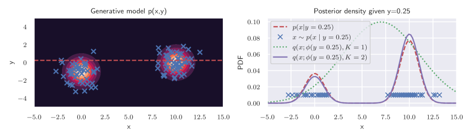
Figure 1: Intuition for Lightweight Inference Compilation (LIC). LIC uses samples $(x_{i},y_{i})\overset{\text{iid}}{\sim}p$ (blue “x” in left) drawn from the joint density $p(x,y)$ to approximate the expected inclusive KL-divergence $\mathbb{E}_{p(y)}D_{\text{KL}}(p(x\mid y)\;\|\;q(x;\phi(y)))$ between the posterior $p(x\mid y)$ and the LIC proposal distribution $q(x;\phi(y))$. For an observation $y=0.25$ (dashed red line in left), the posterior $p(x\mid y=0.25)$ (dashed red line in right) is “approximated” by samples “close” to $y$ (blue “x” in right) to form an empirical inclusive KL-divergence minimized by LIC. As inclusive KL-divergence encourages a mass-covering / mean-seeking fit, the resulting proposal distribution $q(x;\phi(y=0.25),K=1)$ (green dotted line in right) when using a single ($K=1$) Gaussian proposal density covers both modes and can successfully propose moves which cross between the two mixture components. Using a 2-component ($K=2$) GMM proposal density results in $q(x;\phi(y=0.25),K=2)$ (purple solid line in right) which captures both the bi-modality of the posterior as well as the low probability region between the two modes. As a result of sampling the generative model, LIC can discover both posterior modes and their appropriate mixture weights (whereas other state of the art MCMC samplers fail, see fig. 3).

Deriving and implementing samplers has traditionally been a high-effort and application-specific endeavour (Porteous et al.,, 2008; Murray et al.,, 2010), motivating the development of general-purpose probabilistic programming languages (PPLs) where a non-expert can specify a generative model (i.e. joint distribution) $p(\vec{x},\vec{y})$ and the software automatically performs inference to sample latent variables $\vec{x}$ from the posterior $p(\vec{x}\mid\vec{y})$ conditioned on observations $\vec{y}$. While exceptions exist, modern general-purpose PPLs typically implement variational inference (Bingham et al.,, 2019), importance sampling (Wood et al.,, 2014; Le et al.,, 2017), or Monte Carlo Markov Chain (MCMC, Wingate et al., (2011); Tehrani et al., (2020)).

Our work focuses on MCMC. More specifically, we target lightweight Metropolis-Hastings (LMH, Wingate et al., (2011)) within a recently developed declarative PPL called beanmachine (Tehrani et al.,, 2020). The performance of Metropolis-Hastings critically depends on the quality of the proposal distribution used, which is the primary goal of LIC. LIC makes the following contributions:

1. We present a novel implementation of inference compilation (IC) within an open-universe declarative PPL which combines Markov blanket structure with graph neural network architectures

2. We describe how to handle novel data encountered at run-time which was not observed during compilation, which is an issue faced by any implementation of IC supporting open-universe models.

3. We demonstrate LIC’s ability to escape local modes, improved robustness to nuisance random variables, and improvements over state-of-the-art methods across a number of metrics in two industry-relevant applications

1.1 Declarative Probabilistic Programming

To make Bayesian inference accessible to non-exports, PPLs provide user-friendly primitives in high-level programming languages for abstraction and composition in model representation (Goodman,, 2013; Ghahramani,, 2015). Existing PPLs can be broadly classified based on the representation inference is performed over, with declarative PPLs (Lunn et al.,, 2000; Plummer et al.,, 2003; Milch et al.,, 2007; Tehrani et al.,, 2020) performing inference over Bayesian graphical networks and imperative PPLs conducting importance sampling (Wood et al.,, 2014) or MCMC (Wingate et al.,, 2011) on linearized execution traces. Because an execution trace is a topological sort of an instantiated Bayesian network, declarative PPLs preserve additional model structure such as Markov blanket relationships which are lost in imperative PPLs.

Definition 1.1.

The Markov Blanket $\operatorname{MB}(x_{i})$ of a node $x_{i}$ is the minimal set of random variables such that

$$p(x_{i}\mid\vec{x}_{-i},\vec{y}) =p(x_{i}\mid\operatorname{MB}(x_{i}))$$ (1)

In a Bayesian network, $\operatorname{MB}(x_{i})$ consists of the parents, children, and children’s parents of $x_{i}$ (Pearl,, 1987).

1.2 Inference Compilation

Amortized inference (Gershman and Goodman,, 2014) refers to the re-use of initial up-front learning to improve future queries. In context of Bayesian inference (Marino et al.,, 2018; Zhang et al.,, 2018) and IC (Paige and Wood,, 2016; Weilbach et al.,, 2019; Harvey et al.,, 2019), this means using acceleration performing multiple inferences over different observations $\vec{y}$ to amortize a one-time “compilation time.” While compilation in both trace-based IC (Paige and Wood,, 2016; Le et al.,, 2017; Harvey et al.,, 2019) and LIC consists of drawing forward samples from the generative model $p(\vec{x},\vec{y})$ and training neural networks to minimize inclusive KL-divergence, trace-based IC uses the resulting neural network artifacts to parameterize proposal distributions for importance sampling while LIC uses them for MCMC proposers.

1.3 Lightweight Metropolis Hastings

LMH (Wingate et al., (2011); Ritchie et al., 2016b ) updates random variables within a probabilistic model one at a time according to a Metropolis-Hastings rule while keeping all the other variables fixed. While a number of choices for proposal distribution exist, the single-site Gibbs sampler which proposes from eq. 1 enjoys a 100% acceptance probability (Pearl,, 1987) and provides a good choice when available (Lunn et al.,, 2000; Plummer et al.,, 2003). Unfortunately, outside of discrete models they are oftentimes intractable to directly sample so another proposal distribution must be used. LIC seeks to approximate these single-site Gibbs distributions using tractable neural network approximations.

1.4 Related Works

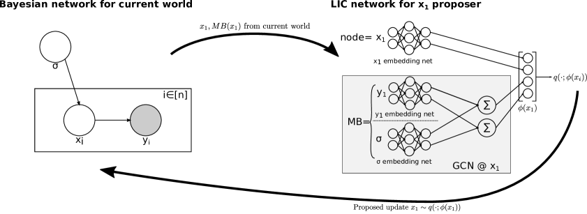
Figure 2: The Markov blankets in the Bayesian network for eq. 3 (left, expressed in plate notation) are available in a declarative PPL, and are used as inputs to LIC. The LIC proposer for node $x_{1}$ (right) is obtained by first performing neural network embedding of $x_{1}$ and every node in its Markov blanket, followed by a graph convolutional network aggregation over the Markov blanket of $x_{1}$. The resulting vectors are then combined to yield a parameter vector $\phi(x_{1})$ for a proposal distribution $q(\cdot;\phi(x_{1}))$ which is then sampled for proposing an update within Metropolis-Hastings.

Prior work on IC in imperative PPLs can be broadly classified based on the order in which nodes are sampled. “Backwards” methods approximate an inverse factorization, starting at observations and using IC artifacts to propose propose parent random variables. Along these lines, Paige and Wood, (2016) use neural autoregressive density estimators but heuristically invert the model by expanding parent sets. Webb et al., (2018) proposes a more principled approach utilizing minimal I-maps and demonstrate that minimality of inputs to IC neural networks can be beneficial; an insight also exploited through LIC’s usage of Markov blankets. Unfortunately, model inversion is not possible in universal PPLs (Le et al.,, 2017).

The other group of “forwards” methods operate in the same direction as the probabilistic model’s dependency graph. Starting at root nodes, these methods produce inference compilation artifacts which map an execution trace’s prefix to a proposal distribution. In Ritchie et al., 2016a , a user-specified model-specific guide program parameterizes the proposer’s architecture and results in more interpretable IC artifacts at the expense of increased user effort. Le et al., (2017) automates this by using a recurrent neural network (RNN) to summarize the execution prefix while constructing a node’s proposal distribution. This approach suffers from well-documented RNN limitations learning long distance dependencies (Hochreiter,, 1998), requiring mechanisms like attention (Harvey et al.,, 2019) to avoid degradation in the presence of long execution trace prefixes (e.g. when nuisance random variables are present).

With respect to prior work, LIC is most similar to the attention-based extension (Harvey et al.,, 2019) of Le et al., (2017). Both methods minimize inclusive KL-divergence empirically approximated by samples from the generative model $p(\vec{x},\vec{y})$, and both methods use neural networks to produce a parametric proposal distribution from a set of inputs sufficient for determining a node’s posterior distribution. However, important distinctions include (1) LIC’s use of a declarative PPL implies Markov blanket relationships are directly queryable and ameliorates the need for also learning an attention mechanism, (2) LIC uses a graph neural network to summarize the Markov blanket rather than a RNN over the execution trace prefix, and (3) LIC can handle open-universe models where novel random variables are encountered at inference time and no embedding network exists.

2 Lightweight Inference Compilation

2.1 Architecture

Figure 2 shows a sketch of LIC’s architecture. For every latent node $x_{i}$, LIC constructs a mapping $(x_{i},\operatorname{MB}(x_{i}))\mapsto\phi(x_{i})$ parameterized by feedforward and graph neural networks to produce a parameter vector $\phi(x_{i})$ for a parametric density estimator $q(\cdot;\phi(x_{i}))$. Every node $x_{i}$ has feedforward “node embedding network” used to map the value of the underlying random variable into a vector space of common dimensionality. The set of nodes in the Markov blanket are then summarized to a fixed-length vector following section 2.1.1, and a feedforward neural network ultimately maps the concatenation of the node’s embedding with its Markov blanket summary to proposal distribution parameters $\phi(x_{i})$.

2.1.1 Dynamic Markov Blanket embeddings

Because a node’s Markov blanket may vary in both its size and elements (e.g. in a GMM, a data point’s component membership may change during MCMC), $\operatorname{MB}(x_{i})$ is a non-static set of vectors (albeit all of the same dimension after node embeddings are applied) and a feed-forward network with fixed input dimension is unsuitable for computing a fixed-length proposal parameter vector $\phi(x_{i})$. Furthermore, Markov blankets (unlike execution trace prefixes) are unordered sets and lack a natural ordering hence use of a RNN as done in Le et al., (2017) is inappropriate. Instead, LIC draws motivation from graph neural networks (Scarselli et al.,, 2008; Dai et al.,, 2016) which have demonstrated superior results in representation learning Bruna et al., (2013) and performs summarization of Markov Blankets following Kipf and Welling, (2016) by defining

$$\phi(x_{i})=\sigma\left(\matr{W}\underset{x_{j}\in\text{MB}(x_{i})}{\square}\frac{1}{\sqrt{\lvert\text{MB}(x_{i})\rvert\lvert\text{MB}(x_{j})\rvert}}f_{j}(x_{j})$$

where $f_{j}(x_{j})$ denotes the output of the node embedding network for node $x_{j}$ when provided its current value as an input, $\square$ is any differentiable permutation-invariant function (summation in LIC’s case), and $\sigma$ is an activation function.

2.1.2 Parameterized density estimation

The resulting parameter vectors $\phi(x_{i})$ of LIC are ultimately used to parameterize proposal distributions $q(x_{i};\phi(\operatorname{MB}(x_{i})))$ for MCMC sampling. For discrete $x_{i}$, LIC directly estimates logit scores over the support. For continuous $x_{i}$, LIC transforms continuous $x_{i}$ to unconstrained space following Carpenter et al., (2017) and models the density using a Gaussian mixture model (GMM). Note that although more sophisticated density estimators such as masked autoregressive flows (Kingma et al.,, 2016; Papamakarios et al.,, 2017) can equally be used.

2.2 Objective Function

To “compile” LIC, parameters are optimized to minimize the inclusive KL-divergence between the posterior distributions and inference compilation proposers: $D_{\text{KL}}(p(\vec{x}\mid\vec{y})\;\|\;q(\vec{x}\mid\vec{y};\phi))$. Consistent with Le et al., (2017), observations $\vec{y}$ are sampled from the marginal distribution $p(\vec{y})$, but note that this may not be representative of observations $\vec{y}$ encountered at inference. The resulting objective function is given by

$$\mathbb{E}_{p(\vec{y})}\left[D_{\text{KL}}(p(\vec{x}\mid\vec{y})\;\|\;q(\vec{x}\mid\vec{y};\phi))\right]$$ (2)

$$=\mathbb{E}_{p(\vec{x},\vec{y})}\left[\log\frac{p(\vec{x}\mid\vec{y})}{q(\vec{x}\mid\vec{y};\phi)}\right]$$

$$\propto\mathbb{E}_{p(\vec{x},\vec{y})}\left[-\log q(\vec{x}\mid\vec{y};\phi)\right]$$

$$\approx\sum_{i=1}^{N}-\log q(\vec{x}\mid\vec{y};\phi),\qquad(\vec{x},\vec{y})\overset{\text{iid}}{\sim}p(\vec{x},\vec{y})$$

$$\eqqcolon\mathcal{L}(\phi)$$

where we have neglected a conditional entropy term independent of $\phi$ and performed Monte-Carlo approximation to an expectation. The intuition for this objective is shown in Figure 1, which shows how samples from $p(\vec{x},\vec{y})$ (left) form an empirical joint approximation where “slices” (at $y=0.25$ in fig. 1) yield posterior approximations which the objective is computed over (right).

2.2.1 Open-universe support / novel data at runtime

Because the number of random variables in an open-universe probabilistic can be unbounded, it is impossible for any finite-time training procedure which relies on sampling the generative model $p(\vec{x},\vec{y})$ to encounter all possible random variables. As a consequence, any implementation of IC within a universal PPL must address the issue of novel data encountered at inference time. This issue is not explicitly addressed in prior work (Le et al.,, 2017; Harvey et al.,, 2019). In LIC’s case, if a node $x_{i}$ does not have an existing LIC artifact $x_{i}\mapsto\phi(x_{i})$ then we fall back to proposing from the parent-conditional prior $q(x_{i};\operatorname{MB}(x_{i}),\phi_{i})=p(x_{i}\mid\operatorname{Pa}(x_{i}))$ (i.e. ancestral sampling).

3 Experiments

To validate LIC’s competitiveness, we conducted experiments benchmarking a variety of desired behaviors and relevant applications. In particular:

• Training on samples from the joint distribution $p(\vec{x},\vec{y})$ should enable discovery of distant modes, so LIC samplers should be less likely to to get “stuck” in a local mode. We validate this in section 3.1 using a GMM mode escape experiment, where we see LIC escape not only escape a local mode but also yield accurate mixture component weights.

• When there is no approximation error (i.e. the true posterior density is within the family of parametric densities representable by LIC), we expect LIC to closely approximate the posterior at least for the range of observations $\vec{y}$ sampled during compilation (eq. 2) with high probability under the prior $p(\vec{y})$. Section 3.2 shows this is indeed the case in a conjugate Gaussian-Gaussian model where a closed form expression for the posterior is available.

• Because Markov blankets can be explicitly queried, we expect LIC’s performance to be unaffected by the presence of nuisance random variables (i.e. random variables which extend the execution trace but are statistically independent from the observations and queried latent variables). This is confirmed in section 3.3 using the probabilistic program from Harvey et al., (2019), where we see trace-based IC suffering an order of magnitude increase in model parameters and compilation time while yielding an effective sample size almost $5\times$ smaller (Figure 5).

• To verify LIC yields competitive performance in applications of interest, we benchmark LIC against other state-of-the-art MCMC methods on a Bayesian logistic regression problem (section 3.4) and on a generalization of the classical eight schools problem (Rubin,, 1981) called $n$-schools (section 3.5) which is used in production at a large internet company for Bayesian meta-analysis Sutton and Abrams, (2001). We find that LIC exceeds the performance of adaptive random walk Metropolis-Hastings (Garthwaite et al.,, 2016) and Newtonian Monte Carlo (Arora et al.,, 2020) and yields comparable performance to NUTS (Hoffman and Gelman,, 2014) despite being implemented in an interpreted (Python) versus compiled (C++) language.

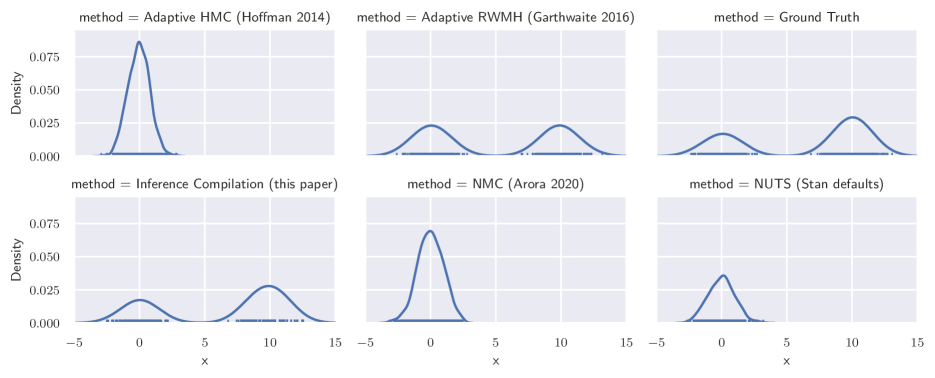
Figure 3: When sampling the bi-modal posterior density from fig. 1, only inference compilation (IC, this paper) and adaptive step-size random walk Metropolis-Hastings (Adaptive RWMH, Garthwaite et al., (2016)) are able to recover both posterior modes. Whereas RWMH’s posterior samples erroneously assign approximately equal probability to both modes, IC’s samples faithfully reproduce the ground truth and yields higher probability for the mode at $x=10$ than the mode at $x=0$.

3.1 GMM mode escape

Consider the multi-modal posterior resulting from conditioning on $y=0.25$ in the 2-dimensional GMM in fig. 1, which is comprised of two Gaussian components with greater mixture probability on the right-hand component and a large energy barrier separating the two components. Because LIC is compiled by training on samples from the joint distribution $p(x,y)$, it is reasonable to expect LIC’s proposers to assign high probability to values for the latent variable $x$ from both modes. In contrast, uncompiled methods such as random walk Metropolis-Hastings (RWMH) and NUTS may encounter difficulty crossing the low-probability energy barrier and be unable to escape the basin of attraction of the mode closest to their initialization.

This intuition is confirmed in fig. 3, which illustrates kernel density estimates of 1,000 posterior samples obtained by a variety of MCMC algorithms as well as ground truth samples. HMC with adaptive step size (Hoffman and Gelman,, 2014), NMC, and NUTS with the default settings as implemented in Stan (Carpenter et al.,, 2017) are all unable to escape the mode they are initialized in. While both LIC and RWMH with adaptive step size escape the local mode, RWMH’s samples erroneously imply equal mixture component probabilities whereas LIC’s samples faithfully reproduce a higher component probability for the right-hand mode.

3.2 Conjugate Gaussian-Gaussian Model

We next consider a Gaussian likelihood with a Gaussian mean prior, a conjugate model with closed-form posterior given by:

$$x\sim\mathcal{N}(0,\sigma_{x}), \qquad y\sim\mathcal{N}(x,\sigma_{y})$$ (3)

$$\Pr[x\mid y,\sigma_{x},\sigma_{y}] \sim\mathcal{N}\left(\frac{\sigma_{y}^{-2}}{\sigma_{x}^{-2}+\sigma_{y}^{-2}}y,\frac{1}{\sigma_{x}^{-2}+\sigma_{y}^{-2}}\right)$$

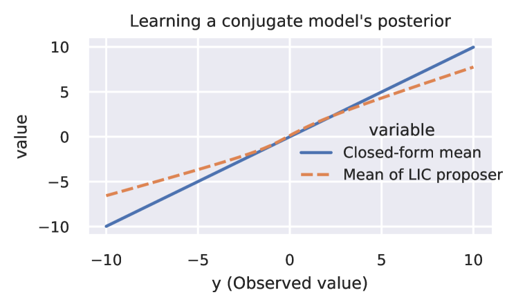
Figure 4: In a conjugate normal-normal model, LIC’s proposal distribution mean (dashed orange line) closely follows the closed-form posterior mean (blue solid line) across a wide range of observed values $y$.

There is minimal approximation error because the posterior density is in the same family as LIC’s GMM proposal distributions and the relationship between the Markov blanket $\operatorname{MB}(x)=\{y\}$ and the posterior mean is a linear function easily approximated (locally) by neural networks. As a result, we expect LIC’s proposal distribution to provide a good approximation to the true posterior and LIC to approximately implement a direct posterior sampler.

To confirm this behavior, we trained LIC with a $K=1$ component GMM proposal density on 1,000 samples and show the resulting LIC proposer’s mean as the observed value $y$ varies in fig. 4. Here $\sigma_{x}=2$ and $\sigma_{y}=0.1$, so the marginal distribution of $y$ (i.e. the observations sampled during compilation in eq. 2) is Gaussian with mean $0$ and standard deviation $\sqrt{\sigma_{x}^{2}+\sigma_{y}^{2}}\approx 2.0025$. Consistent with our expectations, LIC provides a good approximation to the true posterior for observed values $y$ well-represented during training (i.e. with high probability under the marginal $p(y)$). While LIC also provides a reasonable proposer by extrapolation to less represented observed values $y$, it is clear from fig. 4 that the approximation is less accurate. This motivates future work into modifying the forward sampling distribution used to approximate eq. 2 (e.g. “inflating” the prior) as well as adapting LIC towards the distribution of observations $y$ used at inference time.

3.3 Robustness to Nuisance Variables

An important innovation of LIC is its use of a declarative PPL and ability to query for Markov blanket relationships so that only statistically relevant inputs are utilized when constructing proposal distributions. To validate this yields significant improvement over prior work in IC, we reproduced an experiment from Harvey et al., (2019) where nuisance random variables (i.e. random variables which are statistically independent from the queried latent variables/observations whose only purpose is to extend the execution trace) are introduced and the impact on system performance is measured. As trace-based inference compilation utilizes the execution trace prefix to summarize program state, extending the trace of the program with nuisance random variables typically results in degradation of performance due to difficulties encountered by RNN in capturing long range dependencies as well as the production of irrelevant neural network embedding artifacts.

We reproduce trace-based IC as described in Le et al., (2017) using the author-provided PyProb software package, and implement Program 1 from Harvey et al., (2019) with the source code illustrated in LABEL:lst:pyprob where 100 nuisance random variables are added. Note that although nuisance has no relationship to the remainder of the program, the line number where they are instantiated has a dramatic impact on performance. By extending the trace between where x and y are defined, trace-based IC’s RNNs degrade due to difficulty learning a long-range dependency(Hochreiter,, 1998) between the two variables. For LIC, the equivalent program expressed in the beanmachine declarative PPL (Tehrani et al.,, 2020) is shown in LABEL:lst:bm. In this case, the order in which random variable declarations appear is irrelevant as all permutations describe the same probabilistic graphical model.

⬇

1def magnitude(obs):

2 x = sample(Normal(0, 10))

3 for _ in range(100):

4 nuisance = sample(Normal(0, 10))

5 y = sample(Normal(0, 10))

6 observe(

7 obs**2,

8 likelihood=Normal(x**2 + y**2, 0.1))

9 return x

Listing 1: A version of Program 1 from Harvey et al., (2019) to illustrate nuisance random variables

⬇

1class NuisanceModel:

2 @random_variable

3 def x(self):

4 return dist.Normal(0, 10)

5 @random_variable

6 def nuisance(self, i):

7 return dist.Normal(0, 10)

8 @random_variable

9 def y(self):

10 return dist.Normal(0, 10)

11 @random_variable

12 def noisy_sq_length(self):

13 return dist.Normal(self.x()**2 + self.y()**2, 0.1)

Listing 2: The equivalent program in beanmachine, where independencies are explicit in program specification

Figure 5 compares the results between LIC and trace-based IC (Le et al.,, 2017) for this nuisance variable model. Both pyprob’s defaults (1 layer 4 dimension sample embedding, 64 dimension address embedding, 8 dimension distribution type embedding, 10 component GMM proposer, 1 layer 512 dimension LSTM) and LIC’s defaults (used for all experiments in this paper, 1 layer 4 dimension node embedding, 3 layer 8 dimension Markov blanket embedding, 1 layer node proposal network) with a 10 component GMM proposer are trained on 10,000 samples and subsequently used to draw 100 posterior samples. Although model size is not directly comparable due differences in model architecture, pyprob’s resulting models were over $7\times$ larger than those of LIC. Furthermore, despite requiring more than $10\times$ longer time to train, the resulting sampler produced by pyprob yields an effective sample size almost $5\times$ smaller than that produced by LIC.

	# params	compile time	ESS
LIC (this paper)	3,358	44 sec.	49.75
Le et al., (2017)	21,952	472 sec.	10.99

Figure 5: Number of parameters, compilation time (10,000 samples), and effective sample size (100 samples) for inference compilation in declarative (beanmachine, this work) versus imperative (pyprob, Le et al., (2017)) PPLs

3.4 Bayesian Logistic Regression

Consider a Bayesian logistic regression model over $d$ covariates with prior $\vec{\beta}\sim\mathcal{N}_{d+1}(\vec{0}_{d+1},\operatorname{diag}(10,2.5\vec{1}_{d}))$ and likelihood $y_{i}\mid\vec{x}_{i}\overset{\text{iid}}{\sim}\text{Bernoulli}(\sigma(\vec{\beta}^{\top}\vec{x}_{i}))$ where $\sigma(t)=(1+e^{-t})^{-1}$ is the logistic function. This model is appropriate in a wide range of classification problems where prior knowledge about the regression coefficients $\vec{\beta}$ are available.

Figure 6(a) shows the results of performing inference using LIC compared against other MCMC inference methods. All methods yield similar predictive log-likelihoods on held-out test data, but LIC and NUTS yield significantly higher ESS and $\widehat{R}$s closer to $1.0$ suggesting better mixing and more effective sampling.

Figure 6: Results drawing 100 samples across 10 chains (after 1,000 burn-in / adaptation / compilation samples) on two Bayesian inference problems. The top row of each subfigure aggregates over the 10 chains the (left to right) compilation time (time to instantiate the Python class, includes neural network training for LIC and Stan’s C++ codegen and compilation for NUTS), inference time (time from invoking infer() to when sampling terminates), and the predictive log-likelihood (PLL) on held-out test data. The bottom row aggregates over both the 10 chains as well as over all latent variables the (left to right) estimated expected sample size (ESS, higher is better, Geyer, (2011)) and the rank normalized $\widehat{R}$ diagnostic (Rhat, closer to $1$ is better, Vehtari et al., (2020)).

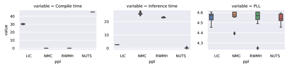
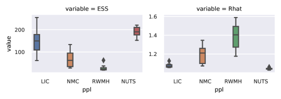
(a) Bayesian logistic regression ($2000$ rows, $10$ features). Both LIC and Stan (NUTS) amortize the upfront compilation cost with accelerated inference times. LIC achieves comparable PLL to NUTS Hoffman and Gelman, (2014) and other methods, and yields ESS comparable to NUTS and higher than any other method. The $\widehat{R}$ of LIC is close to $1$ (similar to NUTS and lower than all other methods).

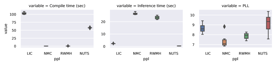
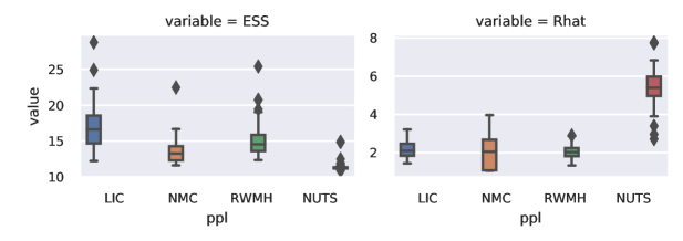
(b) n-schools (1000 schools, 8 states, 5 districts, 5 types). Again, increased compilation times are offset by accelerated inference times. In this case, LIC achieves comparable PLL to NUTS while simultaneously producing higher ESS and lower $\widehat{R}$, suggesting that the resulting posterior samples are less autocorrelated and provide a more accurate posterior approximation.

3.5 n-Schools

The eight schools model (Rubin,, 1981) is a Bayesian hierarchical model originally used to model the effectiveness of schools at improving SAT scores. $n$-schools is a generalization of this model from $8$ to $n$ possible treatments, and is used at a large internet company for performing Bayesian meta-analysis Sutton and Abrams, (2001) to estimate effect sizes across a range of industry-specific applications. Let $K$ denote the total number of schools, $n_{j}$ the number of districts/states/types, and $j_{k}$ the district/state/type of school $k$.

$$\beta_{0} \sim\text{StudentT}(3,0,10)$$

$$\tau_{i} \sim\text{HalfCauchy}(\sigma_{i})\qquad\text{for}~{}i\in[\text{district},\text{state},\text{type}]$$

$$\beta_{i,j} \sim\mathcal{N}(0,\tau_{i})\qquad\text{for}~{}i\in[\text{district},\text{state},\text{type}],j\in[n_{i}]$$

$$y_{k} \sim\mathcal{N}(\beta_{0}+\sum_{i}\beta_{i,j_{k}},\sigma_{k})$$

Figure 6(b) presents results in a format analogous to section 3.4. Here, we see that while both LIC and NUTS yield higher PLLs (with NUTS outperforming LIC in this case), LICs ESS is significantly higher than other compared methods. Additionally, the $\widehat{R}$ of NUTS is also larger than the other methods which suggests that even after 1,000 burn-in samples NUTS has still not properly mixed.

4 Conclusion

We introduced Lightweight Inference Compilation (LIC) for building high quality single-site proposal distributions to accelerate Metropolis-Hastings MCMC. LIC utilizes declarative probabilistic programming to retain graphical model structure and graph neural networks to approximate single-site Gibbs sampling distributions. To our knowledge, LIC is the first proposed method for inference compilation within an open-universe declarative probabilistic programming language and an open-source implementation will be released in early 2021. Compared to prior work, LIC’s use of Markov blankets resolves the need for attention to handle nuisance random variances and yields posterior sampling comparable to state-of-the-art MCMC samplers such as NUTS and adaptive RWMH.

References

- Arora et al., (2020) Arora, N. S., Tehrani, N. K., Shah, K. D., Tingley, M., Li, Y. L., Torabi, N., Noursi, D., Masouleh, S. A., Lippert, E., and Meijer, E. (2020). Newtonian monte carlo: single-site mcmc meets second-order gradient methods. arXiv preprint arXiv:2001.05567.
- Bingham et al., (2019) Bingham, E., Chen, J. P., Jankowiak, M., Obermeyer, F., Pradhan, N., Karaletsos, T., Singh, R., Szerlip, P., Horsfall, P., and Goodman, N. D. (2019). Pyro: Deep universal probabilistic programming. The Journal of Machine Learning Research, 20(1):973–978.
- Bruna et al., (2013) Bruna, J., Zaremba, W., Szlam, A., and LeCun, Y. (2013). Spectral networks and locally connected networks on graphs. arXiv preprint arXiv:1312.6203.
- Carpenter et al., (2017) Carpenter, B., Gelman, A., Hoffman, M. D., Lee, D., Goodrich, B., Betancourt, M., Brubaker, M., Guo, J., Li, P., and Riddell, A. (2017). Stan: A probabilistic programming language. Journal of statistical software, 76(1).
- Dai et al., (2016) Dai, H., Dai, B., and Song, L. (2016). Discriminative embeddings of latent variable models for structured data. In International conference on machine learning, pages 2702–2711.
- Garthwaite et al., (2016) Garthwaite, P. H., Fan, Y., and Sisson, S. A. (2016). Adaptive optimal scaling of metropolis–hastings algorithms using the robbins–monro process. Communications in Statistics-Theory and Methods, 45(17):5098–5111.
- Gershman and Goodman, (2014) Gershman, S. and Goodman, N. (2014). Amortized inference in probabilistic reasoning. In Proceedings of the annual meeting of the cognitive science society, volume 36.
- Geyer, (2011) Geyer, C. (2011). Introduction to markov chain monte carlo. Handbook of markov chain monte carlo, 20116022:45.
- Ghahramani, (2015) Ghahramani, Z. (2015). Probabilistic machine learning and artificial intelligence. Nature, 521(7553):452–459.
- Goodman, (2013) Goodman, N. D. (2013). The principles and practice of probabilistic programming. ACM SIGPLAN Notices, 48(1):399–402.
- Harvey et al., (2019) Harvey, W., Munk, A., Baydin, A. G., Bergholm, A., and Wood, F. (2019). Attention for inference compilation. arXiv preprint arXiv:1910.11961.
- Hochreiter, (1998) Hochreiter, S. (1998). The vanishing gradient problem during learning recurrent neural nets and problem solutions. International Journal of Uncertainty, Fuzziness and Knowledge-Based Systems, 6(02):107–116.
- Hoffman and Gelman, (2014) Hoffman, M. D. and Gelman, A. (2014). The no-u-turn sampler: adaptively setting path lengths in hamiltonian monte carlo. J. Mach. Learn. Res., 15(1):1593–1623.
- Kingma et al., (2016) Kingma, D. P., Salimans, T., Jozefowicz, R., Chen, X., Sutskever, I., and Welling, M. (2016). Improved variational inference with inverse autoregressive flow. In Advances in neural information processing systems, pages 4743–4751.
- Kipf and Welling, (2016) Kipf, T. N. and Welling, M. (2016). Semi-supervised classification with graph convolutional networks. arXiv preprint arXiv:1609.02907.
- Le et al., (2017) Le, T. A., Baydin, A. G., and Wood, F. (2017). Inference compilation and universal probabilistic programming. In Artificial Intelligence and Statistics, pages 1338–1348.
- Lunn et al., (2000) Lunn, D. J., Thomas, A., Best, N., and Spiegelhalter, D. (2000). Winbugs-a bayesian modelling framework: concepts, structure, and extensibility. Statistics and computing, 10(4):325–337.
- Marino et al., (2018) Marino, J., Yue, Y., and Mandt, S. (2018). Iterative amortized inference. arXiv preprint arXiv:1807.09356.
- Milch et al., (2007) Milch, B., Marthi, B., Russell, S., Sontag, D., Ong, D. L., and Kolobov, A. (2007). 1 blog: Probabilistic models with unknown objects. Statistical relational learning, page 373.
- Murray et al., (2010) Murray, I., Adams, R., and MacKay, D. (2010). Elliptical slice sampling. In Proceedings of the thirteenth international conference on artificial intelligence and statistics, pages 541–548.
- Paige and Wood, (2016) Paige, B. and Wood, F. (2016). Inference networks for sequential monte carlo in graphical models. In International Conference on Machine Learning, pages 3040–3049.
- Papamakarios et al., (2017) Papamakarios, G., Pavlakou, T., and Murray, I. (2017). Masked autoregressive flow for density estimation. In Advances in Neural Information Processing Systems, pages 2338–2347.
- Pearl, (1987) Pearl, J. (1987). Evidential reasoning using stochastic simulation of causal models. Artificial Intelligence, 32(2):245–257.
- Plummer et al., (2003) Plummer, M. et al. (2003). Jags: A program for analysis of bayesian graphical models using gibbs sampling. In Proceedings of the 3rd international workshop on distributed statistical computing, volume 124, pages 1–10. Vienna, Austria.
- Porteous et al., (2008) Porteous, I., Newman, D., Ihler, A., Asuncion, A., Smyth, P., and Welling, M. (2008). Fast collapsed gibbs sampling for latent dirichlet allocation. In Proceedings of the 14th ACM SIGKDD international conference on Knowledge discovery and data mining, pages 569–577.
- (26) Ritchie, D., Horsfall, P., and Goodman, N. D. (2016a). Deep amortized inference for probabilistic programs. arXiv preprint arXiv:1610.05735.
- (27) Ritchie, D., Stuhlmüller, A., and Goodman, N. (2016b). C3: Lightweight incrementalized mcmc for probabilistic programs using continuations and callsite caching. In Artificial Intelligence and Statistics, pages 28–37.
- Rubin, (1981) Rubin, D. B. (1981). Estimation in parallel randomized experiments. Journal of Educational Statistics, 6(4):377–401.
- Scarselli et al., (2008) Scarselli, F., Gori, M., Tsoi, A. C., Hagenbuchner, M., and Monfardini, G. (2008). The graph neural network model. IEEE Transactions on Neural Networks, 20(1):61–80.
- Sutton and Abrams, (2001) Sutton, A. J. and Abrams, K. R. (2001). Bayesian methods in meta-analysis and evidence synthesis. Statistical methods in medical research, 10(4):277–303.
- Tehrani et al., (2020) Tehrani, N., Arora, N. S., Li, Y. L., Shah, K. D., Noursi, D., Tingley, M., Torabi, N., Masouleh, S., Lippert, E., Meijer, E., and et al. (2020). Bean machine: A declarative probabilistic programming language for efficient programmable inference. In The 10th International Conference on Probabilistic Graphical Models.
- Vehtari et al., (2020) Vehtari, A., Gelman, A., Simpson, D., Carpenter, B., Bürkner, P.-C., et al. (2020). Rank-normalization, folding, and localization: An improved for assessing convergence of mcmc. Bayesian Analysis.
- Webb et al., (2018) Webb, S., Golinski, A., Zinkov, R., Siddharth, N., Rainforth, T., Teh, Y. W., and Wood, F. (2018). Faithful inversion of generative models for effective amortized inference. In Advances in Neural Information Processing Systems, pages 3070–3080.
- Weilbach et al., (2019) Weilbach, C., Beronov, B., Harvey, W., and Wood, F. (2019). Efficient inference amortization in graphical models using structured continuous conditional normalizing flows.
- Wingate et al., (2011) Wingate, D., Stuhlmüller, A., and Goodman, N. (2011). Lightweight implementations of probabilistic programming languages via transformational compilation. In Proceedings of the Fourteenth International Conference on Artificial Intelligence and Statistics, pages 770–778.
- Wood et al., (2014) Wood, F., Meent, J. W., and Mansinghka, V. (2014). A new approach to probabilistic programming inference. In Artificial Intelligence and Statistics, pages 1024–1032.
- Zhang et al., (2018) Zhang, C., Bütepage, J., Kjellström, H., and Mandt, S. (2018). Advances in variational inference. IEEE transactions on pattern analysis and machine intelligence, 41(8):2008–2026.