Observer-based predictor
for a SIR model with delays

Abstract

We propose an observer for a SIR epidemic model. The observer is then uplifted into a predictor to compensate for time delays in the input and the output. Tuning criteria are given for tuning gains of the predictor, while the estimation-error stability is ensured using Lyapunov-Krasovskii functionals. The predictor’s performance is evaluated in combination with a time-optimal control. We show that the predictor nearly recovers the performance level of the delay-free system.

1 Introduction

Epidemics are a good example of how reality challenges researchers, offering the opportunity to show the strength of existing techniques and develop new ones in fields as varied as medicine, biology, computational sciences, and mathematical system theory.

Epidemiological models have been primarily used for prediction purposes, while mitigation policies are usually decided based on exhaustive simulations. From the perspective of control theory, an epidemic is viewed as a dynamical system with controlled variables. Its model is an instrument for designing a control action that will achieve the desired outcome. Depending on the context, different assumptions on the model and other control objectives can be formulated. Most works focus on vaccination or treatment policies, with the goals expressed in an optimal-control framework [22]. In the context of the current covid pandemic, with vaccines unavailable at present, attention is shifting towards intervention policies based on social distancing measures. Considering the dramatic effect that extended lockdowns have on people and countries economies, a minimum-time control using social distancing measures and considering hospital capacity restrictions was recently presented for the SIR model [1].

The SIR model, which we also consider in this paper, is arguably the simplest epidemiological model. However, it already exhibits many of the nonlinear characteristics that are present in more elaborate models. We make the model more realistic by adding features such as inaccurate and partial state measurements, and input and measurement delays. In recent months, delays in measurements and policy implementation have proved to be critical in the success or failure of government strategies. The former correspond to the time taken for the tests to be carried out, processed, verified, and made available in centralized databases. The latter correspond to the time it takes the population to adopt restrictions such as quarantine, social distancing habits, and mask use.

Due to the prevalence of delays in the feedback loops of control systems and the associated detrimental effects on performance, input and output delays have received sustained attention in the past decades. Some early strategies for compensating the delays are the Smith controller [23], the transformation-based reduction approach [2], and the time-domain predictor-based designs [16]. Based on present state information, predictors based on Cauchy’s formula provide the state ahead of time [3]. They were formally shown to ensure closed-loop stability [14], but their practical implementation reveals instabilities due to neutral phenomena related to the integrals’ discretization in Cauchy’s formula. These issues inspired new proposals such as filtered predictors [18, 13], and truncated predictors [24]. If the present state is not entirely measurable, it can be replaced by an estimation, provided that the system is observable [11].

A recent approach to the compensation of delays consists of modifying an observer to predict future states. It was first introduced for the case of full-state information [19] and later extended to the partial information scenario [15]. This approach, called observer-predictor, suffers from some drawbacks: It loses the exact nature of predictions obtained with Cauchy’s formula and requires the inclusion of extra sub-predictors designed via LMI techniques. However, it has significant advantages: The observer has the same structure as the system (modulo an output injection term), thus avoiding integrals in the prediction formulae. Also, it is readily applicable to the case of partial state information in observable systems, especially when observers are readily available. Systems with state delays [25] or nonlinear systems [7] can be modified easily to successfully compensate for input or output delays.

To tackle the complexity due to partial state availability, delay, and measurement errors, we resort to a wide array of tools available to specialists in the field of control of dynamical systems. For the control, we use a recent optimal law [1]. The objective is not to steer the epidemics towards a desired equilibrium. Instead, the aim is to track an optimal trajectory. As a result, the dynamics for the estimation error are time-varying and time-delayed. The stability of such dynamics is addressed from both the perspective of classical frequency-domain quasipolynomial analysis [20, 17], and from the perspective of time-domain Lyapunov-Krasowskii analysis [9, 8]. In particular, the system’s time-varying nature is taken into account by embedding the system into a model with polytopic uncertainty [4, 10].

In Section 2, we introduce the SIR model and discuss the issues we want to overcome. An ad hoc change of variable allows designing an observer addressing incomplete state information for the delay-free system. In Section 3, this observer is developed into an observer-based predictor for the system with input and output delays. The next two sections are devoted to tuning the observer: A simple criterion to tune the observer gains is given in Section 4, and conditions for the stability of the prediction error dynamics are given in Section 5. The impact of measurement errors is discussed in Section 6. We conclude with some remarks. We show the validity of our approach by discussing a SIR case study along with the paper, which is of interest in its own right.

Allow us to recall some standard notation used in the literature of time-delay systems.

Notation.

$PC([-\eta,0],\mathbb{R}^{n})$ is the set of piece-wise continuous functions defined on the interval $[-\eta,0]$. Consider a time-delay differential equation

$$\dot{\varepsilon}(\tau)=f(\tau,\varepsilon(\tau),\varepsilon(\tau-\eta(\tau)))\;.$$ (1)

The time-varying delay, $\eta(\tau)$, is bounded by $0<\eta(\tau)\leq\bar{\eta}$. Given an initial function $\varphi\in PC([-\eta(0),0],\mathbb{R}^{n})$ the solution is denoted by $\varepsilon(\tau,\varphi)$. The restriction of $\varepsilon(\tau,\varphi)$ on the interval $[\tau-\eta(\tau),\tau]$ is denoted by

$$\varepsilon_{\tau}(\varphi):\theta\mapsto\varepsilon(\tau+\theta,\varphi)\;,\quad\theta\in[-\eta(\tau),0]\;.$$

We will make use of the trivial function $0_{\bar{\eta}}:\theta\mapsto 0$, $\theta\in[-\bar{\eta},0]$. We use the Euclidean norm $\|\cdot\|$ for vectors and the corresponding induced norm for matrices. For $\varphi\in PC([-\eta,0],\mathbb{R}^{n})$ we use the norm

$$\|\varphi\|_{\eta}=\underset{\theta\in[-\eta,0]}{\sup}\|\varphi(\theta)\|\;.$$

The notation $Q>0$ means that the symmetric matrix $Q$ is positive definite.

2 Problem statement

We consider a state-space SIR model

$$\frac{\mathrm{d}}{\mathrm{d}t}S(t) =-\beta(t-h_{1})S(t)I(t)$$

$$\frac{\mathrm{d}}{\mathrm{d}t}I(t) =(\beta(t-h_{1})S(t)-\gamma)I(t)$$

$$y(t) =I(t-h_{2})\;.$$

Here, $S>0$, $I>0$ denote the susceptible and the infected, respectively. The model is normalized, hence $S+I\leq 1$. The transmission rate, $\beta\in[\beta_{\min},\beta_{\max}]$ with $\beta_{\max}>\beta_{\min}>0$, can be controlled by applying social distancing measures, but such measures take effect $h_{1}$ units of time later. The only information available at time $t$ is the number of infected people at time $t-h_{2}$. The recovery/death rate, $\gamma>0$, and the time delays, $h_{1},h_{2}$, are assumed to be known.

The are of course more sophisticated models. It is possible to include exposed individuals (infected but not infectious), to distinguish between symptomatic and asymptomatic, dead and recovered, etc. However, for epidemics the parameters of which have large levels of uncertainty, such as covid-19, a simple model with fewer parameters is preferable, as long as it is able to reproduce the main features of the epidemics (hospital saturation, lock-down effects, herd immunity, and so forth). A simpler model is also preferable when the objective is to devise decision strategies, rather that simulating long-term behavior.

Using only the history of $y$, we wish to produce predictions $\hat{S},\hat{I}$ such that

$$\lim_{t\to\infty}(\hat{S}(t)),\hat{I}(t))=(S(t+h_{1}),I(t+h_{1}))\;.$$

Our motivation is that, if we have a feedback $\beta^{*}(S,I)$ that is known to perform correctly on the system without delays, we can set $\beta=\beta^{*}(\hat{S},\hat{I})$ and expect to recover a similar performance.

For concreteness, we consider the optimal-time control strategy described by Angulo et al [1]. For the SIR model, the basic (unmitigated) reproduction number is computed as $R_{0}=\beta_{\max}/\gamma$, while the controlled (mitigated) reproduction number is $R_{c}=\beta_{\min}/\gamma$. Suppose that the health system capacity of a given city is limited to $I_{\max}$ infected people. The strategy that ensures $I(t)\leq I_{\max}$ and achieves herd immunity in a minimal time is

$$\beta^{\star}(S,I)=\begin{cases}\beta_{\max}&\text{if $I<\Phi(S)$ or $S\leq 1/R_{0}$}\\ \beta_{\min}&\text{otherwise}\end{cases}$$ (2)

with

$$\Phi(S)=\begin{cases}I_{\max}+\frac{1}{R_{c}}\ln\left(\frac{S}{S^{\star}}\right)-(S-S^{\star})&\text{if $S^{\star}\leq S\leq 1$}\\ I_{\max}&\text{if $\frac{1}{R_{0}}\leq S\leq S^{\star}$}\end{cases}$$

and

$$S^{\star}=\min\left\{\frac{1}{R_{c}},1\right\}\;.$$

We consider a recovery rate $\gamma=1/7$ with time units given in days [1]. For illustration purposes, we consider the case of Mexico City. The number of ICU beds is such that $I_{\max}=12.63\times 10^{-3}$ (see [1]). We take the reproduction numbers as $R_{0}=1.7$ and $R_{c}=1.1$ . This gives

$$\beta_{\max}=1.7/7\quad\text{and}\quad\beta_{\max}=1.1/7\;.$$

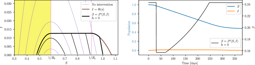
Figure 1: Phase-plane of the model under the optimal feedback law (2) (left). The trajectory with thick line is depicted on the right (blue and orange, scale shown on the left axis). The control action is also included (black, scale shown on the right axis).

The optimal response, achieved with full state-feedback in the absence of delays, is shown in Fig. 1. The optimal strategy is to allow the epidemic to run free until it reaches the sliding curve $I=\Phi(S)$. The state is then driven along this curve towards the region of herd immunity (yellow rectangle) where the intervention finally stops.

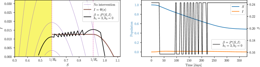
Figure 2: Trajectory corresponding to the feedback law (2) subject to a delay of $h_{1}=3$ days that ultimately results in chattering.

Suppose now that there is a delay of $h_{1}=3$ days in the control action. Fig. 2 confirms the appearance of the so-called chattering effect, which should not be surprising given the discontinuous nature of (2). We can expect the performance of the closed-loop system to deteriorate even further when only the number of infected people is available for measurement, and when such measurements are also subject to important delays. The objective of the predictor, developed in the following section, is to mitigate these unfavorable effects.

3 Observer-based predictor

To attain our objective we follow the approach in which an observer for the delay-free system is constructed in a first step, and then developed into a predictor in a second one [19, 25, 6].

3.1 Delay-free observer

We begin by making the temporary assumption $h_{1}=h_{2}=0$. Note that, by setting $x_{1}=\ln(y)$ and $x_{2}=S$, we obtain the model

$$\frac{\mathrm{d}}{\mathrm{d}t}x_{1}(t) =\beta(t)x_{2}(t)-\gamma$$

$$\frac{\mathrm{d}}{\mathrm{d}t}x_{2}(t) =\beta(t)\rho(x(t))$$

with $\rho(x)=-x_{2}e^{x_{1}}$. The main advantage over the original model is that the first equation is affine in the state. We can then write the simple observer

$$\frac{\mathrm{d}}{\mathrm{d}t}\breve{x}_{1}(t) =\beta(t)\left(\breve{x}_{2}(t)+\alpha_{1}(x_{1}(t)-\breve{x}_{1}(t))\right)-\gamma$$

$$\frac{\mathrm{d}}{\mathrm{d}t}\breve{x}_{2}(t) =\beta(t)\left(\rho(\breve{x}(t))+\alpha_{2}(x_{1}(t)-\breve{x}_{1}(t))\right)\;,$$

where $\alpha_{1},\alpha_{2}$ will be defined below (Proposition 1). Consider the error $\tilde{x}=x-\breve{x}$. By using the expansion

$$\rho(\breve{x})=\rho(x)+\begin{pmatrix}-x_{2}e^{x_{1}}&-e^{x_{1}}\end{pmatrix}\tilde{x}+\mathcal{O}(\|\tilde{x}\|^{2})\;,$$

we can write the error dynamics as

$$\frac{\mathrm{d}}{\mathrm{d}t}\begin{pmatrix}\tilde{x}_{1}(t)\\ \tilde{x}_{2}(t)\end{pmatrix}=\beta(t)A(t)\begin{pmatrix}\tilde{x}_{1}(t)\\ \tilde{x}_{2}(t)\end{pmatrix}+\mathcal{O}(\|\tilde{x}(t)\|^{2})$$ (3)

with

$$A(t)=\begin{pmatrix}-\alpha_{1}&1\\ -\alpha_{2}-S(t)I(t)&-I(t)\end{pmatrix}\;.$$

Note that, since we are linearizing the estimation error around a trajectory (rather than an equilibrium), the linearized system is time-varying. Fortunately, we can ensure its stability with a simple quadratic Lyapunov function.

Proposition 1.

Set

$$\alpha_{2}>\frac{\alpha_{1}^{2}+1}{4\sqrt{2}\alpha_{1}-1}\;,\quad\alpha_{1}>\frac{1}{4\sqrt{2}}\;.$$ (4)

Then (3) is quadratically stable.

Proof.

Consider the candidate Lyapunov function $V(\tilde{x})=\tilde{x}^{\top}P\tilde{x}$ with $P=P^{\top}>0$ the solution of the Lyapunov equation

$$P\begin{pmatrix}-\alpha_{1}&1\\ -\alpha_{2}&0\end{pmatrix}+\begin{pmatrix}-\alpha_{1}&-\alpha_{2}\\ 1&0\end{pmatrix}P=-\begin{pmatrix}1&0\\ 0&1\end{pmatrix}\;,$$

that is,

$$P=\frac{1}{2\alpha_{1}\alpha_{2}}\begin{pmatrix}\alpha_{2}^{2}+\alpha_{2}&-\alpha_{1}\alpha_{2}\\ -\alpha_{1}\alpha_{2}&\alpha_{1}^{2}+\alpha_{2}+1\end{pmatrix}\;.$$

The time-derivative of $V$ along the trajectories of (3) is

$$\dot{V}(\tilde{x}(t))=-\frac{\beta(t)}{2\alpha_{1}\alpha_{2}}\tilde{x}^{\top}(t)Q(S(t),I(t))\tilde{x}(t)+\mathcal{O}(\|\tilde{x}(t)\|^{3})$$

with

$$Q(S,I)=\begin{pmatrix}2(1-SI)\alpha_{1}\alpha_{2}&(\alpha_{1}^{2}+\alpha_{2}+1)SI-\alpha_{1}\alpha_{2}I\\ (\alpha_{1}^{2}+\alpha_{2}+1)SI-\alpha_{1}\alpha_{2}I&2\left(\alpha_{1}\alpha_{2}+(\alpha_{1}^{2}+\alpha_{2}+1)I\right)\end{pmatrix}\;.$$

The restrictions $(S,I)\in[0,1]^{2}$, $S+I\leq 1$ imply that $SI\leq 1/4$, so the first leading principal minor of $Q(S,I)$, $2(1-SI)\alpha_{1}\alpha_{2}$, is strictly positive. Regarding the second leading principal minor, we have

$$|Q(S,I)|=\alpha_{1}^{2}\alpha_{2}^{2}\left(4(1-SI)-I^{2}\right)+\alpha_{1}\alpha_{2}(\alpha_{1}^{2}+\alpha_{2}+1)(4-2SI)I\\ -(\alpha_{1}^{2}+\alpha_{2}+1)^{2}S^{2}I^{2}\;.$$

Using again $SI\leq 1/4$ we obtain the bound

$$|Q(S,I)|\geq 2\alpha_{1}^{2}\alpha_{2}^{2}-\frac{1}{16}(\alpha_{1}^{2}+\alpha_{2}+1)^{2}\;.$$

Finally, the condition (4) ensures that $|Q(S,I)|>0$, so that $V$ is indeed a Lyapunov function. ∎

In the original coordinates, the observer takes the form

$$\frac{\mathrm{d}}{\mathrm{d}t}\breve{S}(t) =-\beta(t)\left(\breve{S}(t)\breve{I}(t)-\alpha_{2}\ln\left(\frac{y(t)}{\breve{I}(t)}\right)\right)$$ (5)

$$\frac{\mathrm{d}}{\mathrm{d}t}\breve{I}(t) =\left(\beta(t)\breve{S}(t)-\gamma+\beta(t)\alpha_{1}\ln\left(\frac{y(t)}{\breve{I}(t)}\right)\right)\breve{I}(t)\;.$$

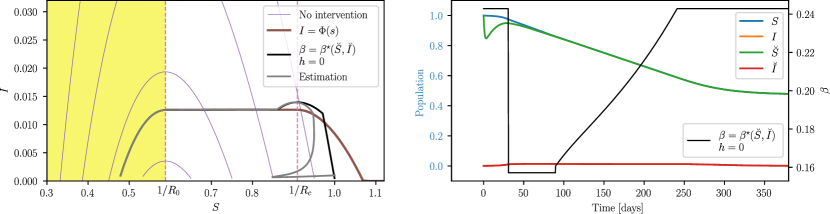
Figure 3: True and estimated trajectories under the feedback law $\beta=\beta^{\star}(\breve{S},\breve{I})$, with no delays.

A simulation of the observer’s performance is shown in Fig. 3. The observer gains, $\alpha^{\top}=\begin{pmatrix}\alpha_{1}&\alpha_{2}\end{pmatrix}=\begin{pmatrix}4&1\end{pmatrix}$ were chosen to satisfy (4). At first, the incidence of infection exceeds $I_{\max}$ by about 11 %, but then the epidemics behave as desired.

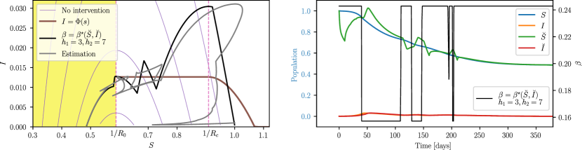
Figure 4: True and estimated trajectories under the feedback law $\beta=\beta^{\star}(\breve{S},\breve{I})$ with $h_{1}=3$ and $h_{2}=7$ days.

Consider again the input delay $h_{1}=3$ days, and suppose now there is a measurement delay of $h_{2}=7$ days [5]. The combined effect of both delays is disastrous. As illustrated in Fig. 4, the hospital capacity is exceeded by 140 %. This motivates the design of the predictor presented in the sequel.

3.2 Predictor

Let us rewrite the observer in the original coordinates and remove the zero-delays assumption. This gives the predictor

$$\frac{\mathrm{d}}{\mathrm{d}t}\hat{S}(t) =-\beta(t)\left(\hat{S}(t)\hat{I}(t)-\alpha_{2}\ln\left(\frac{y(t)}{\hat{I}(t-h)}\right)\right)$$ (6)

$$\frac{\mathrm{d}}{\mathrm{d}t}\hat{I}(t) =\left(\beta(t)\hat{S}(t)-\gamma+\beta(t)\alpha_{1}\ln\left(\frac{y(t)}{\hat{I}(t-h)}\right)\right)\hat{I}(t)$$

with $h=h_{1}+h_{2}$. Considering that $y(t)=I(t-h_{2})$, the error variables

$$\tilde{x}_{1}(t) =\ln\left(\frac{I(t)}{\hat{I}(t-h_{1})}\right)$$ (7)

$$\tilde{x}_{2}(t) =S(t)-\hat{S}(t-h_{1})$$

evolve according to the dynamics

$$\begin{aligned} \frac{\mathrm{d}}{\mathrm{d}t}\tilde{x}_{1}(t)&=\beta(t-h_{1})\left(S(t)-\hat{S}(t-h_{1})-\alpha_{1}\ln\left(\frac{I(t-h)}{\hat{I}(t-h-h_{1})}\right)\right)\\ \frac{\mathrm{d}}{\mathrm{d}t}\tilde{x}_{2}(t)&=\beta(t-h_{1})\Bigg{(}-\alpha_{2}\ln\left(\frac{I(t-h)}{\hat{I}(t-h-h_{1})}\right)+\hat{S}(t-h_{1})\hat{I}(t-h_{1})-S(t)I(t)\Bigg{)}\end{aligned}\;.$$ (8)

Since $\hat{I}(t-h_{1})=e^{-\tilde{x}_{1}(t)}I(t)$ and $\hat{S}(t-h_{1})=S(t)-\tilde{x}_{2}(t)$, we have

$$\frac{\mathrm{d}}{\mathrm{d}t}\tilde{x}_{1}(t) =\beta(t-h_{1})\left(-\alpha_{1}\tilde{x}_{1}(t-h)+\tilde{x}_{2}(t)\right)$$ (9)

$$\frac{\mathrm{d}}{\mathrm{d}t}\tilde{x}_{2}(t) =\beta(t-h_{1})\left(-\alpha_{2}\tilde{x}_{1}(t-h)+\psi(S(t),I(t),\tilde{x}(t))\right)$$

with

$$\psi(S,I,\tilde{x})=((S-\tilde{x}_{2})e^{-\tilde{x}_{1}}-S)I\;.$$ (10)

System (9) can be written in the general form

$$\frac{\mathrm{d}}{\mathrm{d}t}\tilde{x}(t)=\beta(t-h_{1})\left[A_{0}(t)\tilde{x}(t)+A_{1}\tilde{x}(t-h)+G(t,\tilde{x}(t))\tilde{x}(t)\right]$$ (11)

where the matrices are defined by

$$A_{0}(t)=\begin{pmatrix}0&1\\ -S(t)I(t)&-I(t)\end{pmatrix}\;,\quad A_{1}=\begin{pmatrix}-\alpha_{1}&0\\ -\alpha_{2}&0\end{pmatrix}$$ (12)

and

$$G(t,\tilde{x})=\begin{pmatrix}0&0\\ G_{21}(t,\tilde{x})&G_{22}(t,\tilde{x})\end{pmatrix}=\mathcal{O}(\|\tilde{x}\|)$$

with

$$\begin{aligned} G_{21}(t,\tilde{x})&=-S(t)I(t)\frac{e^{-\tilde{x}_{1}}+\tilde{x}_{1}-1}{\tilde{x}_{1}}\\ G_{22}(t,\tilde{x})&=-I(t)(e^{-\tilde{x}_{1}}-1)\end{aligned}\;.$$ (13)

Since $\beta$ multiplies all the right-hand side of (11), we can do away with it by rescaling time, much in the spirit of perturbation theory [12, Ch. 10]. Define the new time-scale

$$\tau=g(t)=\int_{0}^{t}\beta(s-h_{1})\mathrm{d}s\;.$$

Since $\beta$ is strictly positive, $g$ is strictly increasing, invertible and $\tau$ is indeed a time-scale. Let us define the new state $\varepsilon(\tau)=\tilde{x}(g^{-1}(\tau))$ and note that, by the Inverse Function Theorem, we have

$$\frac{\mathrm{d}}{\mathrm{d}\tau}g^{-1}(\tau)=\frac{1}{\frac{\mathrm{d}}{\mathrm{d}t}g(t)}\Bigg{|}_{t=g^{-1}(\tau)}=\frac{1}{\beta(t-h_{1})}\Bigg{|}_{t=g^{-1}(\tau)}\;.$$ (14)

Applying the chain rule and (14), we see that the new state evolves according to

$$\frac{\mathrm{d}}{\mathrm{d}\tau}\varepsilon(\tau)=\frac{1}{\beta(t-h_{1})}\frac{\mathrm{d}}{\mathrm{d}t}\tilde{x}(t)\Big{|}_{t=g^{-1}(\tau)}\;,$$

that is,

$$\dot{\varepsilon}(\tau)=B_{0}(\tau)\varepsilon(\tau)+B_{1}\varepsilon(\tau-\eta(\tau))+H(\tau,\varepsilon(\tau))\varepsilon(\tau)$$ (15)

with

$$B_{0}(\tau)=A_{0}(g^{-1}(\tau))\;,\quad B_{1}=A_{1}\;,\quad H(\tau,\varepsilon)=G(g^{-1}(\tau),\varepsilon)$$

and

$$\eta(\tau)=\tau-g(g^{-1}(\tau)-h)\;.$$

The last equation follows from the condition

$$\varepsilon(\tau-\eta(\tau))=\varepsilon(g(g^{-1}(\tau)-h))=\tilde{x}(g^{-1}(\tau)-h))\;.$$

Observe that $\beta_{\min}h\leq\tau-g(t-h)=\int_{t-h}^{t}\beta(s-h_{1})\mathrm{d}s\leq\beta_{\max}h$, so the time-varying delay is bounded by

$$\beta_{\min}h\leq\eta(\tau)\leq\beta_{\max}h=\bar{\eta}\;.$$

4 Tuning the predictor gains

There are two main difficulties in establishing the stability of (15): The time-varying nature of $B_{0}$, and the presence of the delayed state. The former difficulty will be addressed by formulating (15) in the framework of polytopic differential inclusions [4, Ch. 5]. In order to do so, we will focus on the state-space rectangle $[0,1]\times[0,\bar{I}]$, where $I_{\max}\leq\bar{I}\leq 1$. When the state is restricted to such rectangle, $B_{0}$ varies within a fixed polytope of matrices, i.e.,

$$B_{0}(t)\in\operatorname{Co}\{C_{1},C_{2},C_{3}\}\;,$$ (16)

where

$$C_{1}=\begin{pmatrix}0&1\\ 0&0\end{pmatrix}\;,\quad C_{2}=\begin{pmatrix}0&1\\ 0&-\bar{I}\end{pmatrix}\;,\quad C_{3}\begin{pmatrix}0&1\\ -\bar{I}&-\bar{I}\end{pmatrix}$$

and $\operatorname{Co}$ stands for convex closure, that is,

$$\operatorname{Co}\{C_{1},C_{2},C_{3}\}=\left\{\sum_{i=1}^{3}c_{i}\cdot C_{i}\mid c_{i}\geq 0,\,\sum_{i=1}^{3}c_{i}=1\right\}\;.$$

An obvious necessary condition for the stability of the polytopic model (15)-(16) is the stability of its linearized vertices,

$$\dot{\varepsilon}(\tau)=C_{i}\varepsilon(\tau)+B_{1}\varepsilon(\tau-\bar{\eta})\;,\quad i=1,2,3.$$

The characteristic equations of the vertices are

$$\begin{aligned} p_{1}(s)&=s^{2}+\left(s\alpha_{1}+\alpha_{2}\right)e^{-\bar{\eta}s}\\ p_{2}(s)&=s^{2}+\left((s+\bar{I})\alpha_{1}+\alpha_{2}\right)e^{-\bar{\eta}s}+s\bar{I}\\ p_{3}(s)&=s^{2}+\left((s+\bar{I})\alpha_{1}+\alpha_{2}\right)e^{-\bar{\eta}s}+(s+1)\bar{I}\end{aligned}\;.$$ (17)

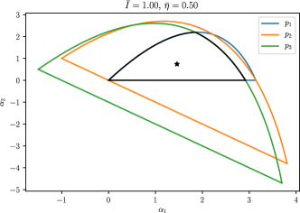
Figure 5: Stability/instability boundaries of the quasipolynomials (17) in the space of parameters $(\alpha_{1},\alpha_{2})$ for $\bar{I}=1$ and $\bar{\eta}=0.5$. The boundary of the intersection of the three regions is depicted in black.

We will work out the stability/instability boundaries of these quasipolynomials in the space of parameters $(\alpha_{1},\alpha_{2})$. According to the D-partition method [20], these boundaries correspond to roots crossing the imaginary axis of the complex plane. When the crossing root is real ($s=0$), the boundaries are

$$p_{1}:\quad\alpha_{2} =0$$

$$p_{2}:\quad\alpha_{2} =-\alpha_{1}\bar{I}$$

$$p_{3}:\quad\alpha_{2} =-(\alpha_{1}+1)\bar{I}\;.$$

If a crossing root is imaginary $(s=j\omega)$, the boundaries satisfy

$$p_{1} :\quad\begin{pmatrix}\omega\sin(\omega\bar{\eta})&\cos(\omega\bar{\eta})\\ \omega\cos(\omega\bar{\eta})&-\sin(\omega\bar{\eta})\end{pmatrix}\alpha=\begin{pmatrix}\omega^{2}\\ 0\end{pmatrix}$$

$$p_{2} :\quad\begin{pmatrix}\omega\sin(\omega\bar{\eta})+\bar{I}\cos(\omega\bar{\eta})&\cos(\omega\bar{\eta})\\ \omega\cos(\omega\bar{\eta})-\bar{I}\sin(\omega\bar{\eta})&-\sin(\omega\bar{\eta})\end{pmatrix}\alpha=\begin{pmatrix}\omega^{2}\\ -\omega\bar{I}\end{pmatrix}$$

$$p_{3} :\quad\begin{pmatrix}\omega\sin(\omega\bar{\eta})+\bar{I}\cos(\omega\bar{\eta})&\cos(\omega\bar{\eta})\\ \omega\cos(\omega\bar{\eta})-\bar{I}\sin(\omega\bar{\eta})&-\sin(\omega\bar{\eta})\end{pmatrix}\alpha=\begin{pmatrix}\omega^{2}-\bar{I}\\ -\omega\bar{I}\end{pmatrix}$$

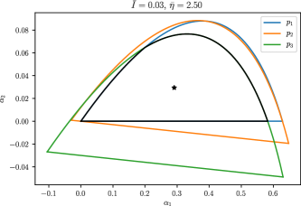
Figure 6: Stability/instability boundaries of the quasipolynomials (17) in the space of parameters $(\alpha_{1},\alpha_{2})$ for $\bar{I}=0.03$ and $\bar{\eta}=2.5$. The boundary of the intersection of the three regions is depicted in black.

The form and disposition of the stability regions depend on $\bar{\eta}$ and $\bar{I}$. Figure 5 shows their boundaries for a relatively small delay, $\bar{\eta}=0.5$, and the largest incidence, $\bar{I}=1$. Figure 6 shows the boundaries of the stability regions for a larger delay, $\bar{\eta}=2.5$, but a smaller incidence, $\bar{I}=0.03$. Since stability of the three vertices is a necessary condition for the stability of (15)-(16), we require $\alpha$ to be placed at the intersection of the three regions (boundaries drawn in black), for example, at an approximate centroid of the intersection (marked with $\star$).

5 Stability of the predictor

Setting $\alpha$ as described in the previous section, i.e., at the intersection of the stability regions, only ensures that a necessary condition for stability is satisfied. We will now exploit the polytopic nature of (3) and the fact that stabilty is ensured by the existence of a Lyapunov-Krasowskii functional that is common to all the vertices of the polytope.

We will begin by summarizing a general assertion from the book by Fridman [8].

Lemma 1.

Consider the candidate Lyapunov-Krasowskii functional

$$V(\varepsilon_{\tau})=\varepsilon^{\top}(\tau)P\varepsilon(\tau)+\int_{\tau-\bar{\eta}}^{\tau}\varepsilon^{T}(s)S\varepsilon(s)\mathrm{d}s+\bar{\eta}\int_{-\bar{\eta}}^{0}\int_{\tau+\theta}^{\tau}\dot{\varepsilon}^{\top}(s)R\dot{\varepsilon}(s)\mathrm{d}s\mathrm{d}\theta$$ (18)

with $P>0$, $R\geq 0$ and $S\geq 0$. Define

$$E(\tau)=\begin{pmatrix}\varepsilon(\tau)&\dot{\varepsilon}(\tau)&\varepsilon(\tau-\bar{\eta})&\varepsilon(\tau-\eta(\tau))\end{pmatrix}^{\top}\;.$$

The time derivative of $V$ satisfies

$$\dot{V}(\varepsilon_{\tau})\leq E(\tau)^{\top}\begin{pmatrix}S-R&P&0&R\\ \star&\bar{\eta}^{2}R&0&0\\ \star&\star&-(S+R)&0\\ \star&\star&\star&-2R\end{pmatrix}E(\tau)\;,$$ (19)

where the terms $\star$ are such that the overall matrix is symmetric.

The lemma is easily proved by differentiating $V$ and applying Jensen’s lemma [8, Ch. 3].

Theorem 1.

Let

$$Q(C;P,R,S,P_{2},P_{3})=\\ \begin{pmatrix}C^{T}P_{2}+P_{2}^{T}C+S-R&P-P_{2}^{T}+C^{T}P_{3}&0&P_{2}^{T}B_{1}+R\\ \star&-P_{3}-P_{3}^{T}+\bar{\eta}^{2}R&0&P_{3}^{T}B_{1}\\ \star&\star&-(S+R)&R\\ \star&\star&\star&-2R\end{pmatrix}\;,$$ (20)

where $C,P,R,S,P_{2}$ and $P_{3}$ are $2\times 2$ matrices. Suppose that there exists $P>0$, $R\geq 0$, $S\geq 0$ and $P_{2}$, $P_{3}$ such that

$$Q(C_{i},P,R,S,P_{2},P_{3})<0\;,\quad i=1,2,3\;.$$ (21)

Then, the trivial solution of the observer error-dynamics (15) is asymptotically stable.

Proof.

The proof follows the descriptor approach [8], but we pay special attention to the nonlinear terms in (15) and incorporate the time-varying nature of the system. Consider again (18) and note that, for any $P_{2},P_{3}\in\mathbb{R}^{2\times 2}$,

$$2\left(\varepsilon(\tau)^{\top}P_{2}^{\top}+\dot{\varepsilon}(\tau)^{\top}P_{3}^{\top}\right)\cdot\big{(}B_{0}(\tau)\varepsilon(\tau)+B_{1}\varepsilon(\tau-\eta(\tau))\\ +H(\tau,\varepsilon(\tau))\varepsilon(\tau)-\dot{\varepsilon}(\tau)\big{)}=0$$

or, in matrix form,

$$E(\tau)^{\top}\begin{pmatrix}B_{0}(\tau)^{\top}P_{2}+P_{2}^{\top}B_{0}(\tau)&-P_{2}^{\top}+B_{0}(\tau)^{\top}P_{3}&0&P_{2}^{\top}B_{1}\\ \star&-P_{3}-P_{3}^{\top}&0&P_{3}^{\top}B_{1}\\ \star&\star&0&0\\ \star&\star&\star&0\\ \end{pmatrix}E(\tau)\\ +2\left(\varepsilon(\tau)^{\top}P_{2}^{\top}+\dot{\varepsilon}(\tau)^{\top}P_{3}^{\top}\right)\cdot H(\tau,\varepsilon(\tau))\cdot\varepsilon(\tau)=0\;.$$ (22)

Observe that

$$2\left(\varepsilon(\tau)^{\top}P_{2}^{\top}+\dot{\varepsilon}(\tau)^{\top}P_{3}^{\top}\right)\cdot H(\tau,\varepsilon(\tau))\cdot\varepsilon(\tau)=\mathcal{O}(\|E(\tau)\|^{3})\;,$$

so adding (22) to (19) gives

$$\dot{V}(\varepsilon_{\tau})\leq-E^{\top}(\tau)Q(B_{0}(t);P,R,S,P_{2},P_{3})E(\tau)+\mathcal{O}(\|E(\tau)\|^{3})\;.$$

Because of (16), there exists continuous real-valued functions $c_{i}$ such that

$$B_{0}(\tau)=\sum_{i=1}^{3}c_{i}(\tau)C_{i}\;,\quad c_{i}(\tau)\geq 0\;,\quad\sum_{i=1}^{3}c_{i}(\tau)\equiv 1\;.$$

Since $C$ appears affinely in (20), we have [8, Remark 3.6]

$$\dot{V}(\varepsilon_{\tau})\leq-\sum_{i=1}^{3}c_{i}(\tau)E^{\top}(\tau)Q(C_{i};P,R,S,P_{2},P_{3})E(\tau)+\mathcal{O}(\|E(\tau)\|^{3})\;.$$

By (21), the derivative of $V$ is negative definite in a neighborhood of the origin and asymptotic stability follows. ∎

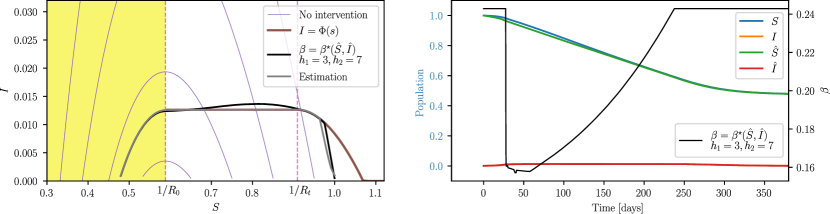
Figure 7: True and estimated trajectories under the feedback law $\beta=\beta^{\star}(\hat{S},\hat{I})$, with $h_{1}=3$ and $h_{2}=7$ days.

For our example, we take a conservative approach and set

$$\bar{\eta}=5>(h_{1}+h_{2})\beta_{\max}=2.4$$

and $\bar{I}=30\times 10^{-3}$ (recall that $I_{\max}=12.63\times 10^{-3}$). The gain $\alpha=\begin{pmatrix}0.115&0.005\end{pmatrix}$ lays within the intersection of the stability regions of $p_{1}$, $p_{2}$ and $p_{3}$.

The LMI (21) was solved using SCS [21]. A solution is

$$P=\begin{pmatrix}51.1&-140.6\\ -140.6&979.2\end{pmatrix}\;,\quad R=S=\begin{pmatrix}16.3&-0.6\\ -0.6&3.3\end{pmatrix}$$

and

$$P_{2}=P_{3}=\begin{pmatrix}42.3&-85.3\\ -140.5&984.4\end{pmatrix}\;,$$

so the prediction error converges to zero asymptotically. This is illustrated in Fig. 7. The hospital capacity is now exceeded by only 7.8 %.

6 On the effect of measurement errors

A frequent situation in epidemics is poor output variable measurement, mainly due to underregistration. A sound assumption is that the output is proportional to the measured variable, $I(t-h_{2})$. The proportion may be time-varying but always less than 1. It is described as

$$y(t)=I(t-h_{2})m(t-h_{2})$$

with

$$m(t)\in[1-\delta,1]\;,\quad 0\leq\delta<1\;.$$ (23)

The logarithmic term in the prediction error dynamics (8) is now

$$\ln\left(\frac{y(t-h_{1})}{\hat{I}(t-h-h_{1})}\right)=\ln\left(\frac{I(t-h)m(t-h)}{\hat{I}(t-h-h_{1})}\right)\\ =\ln\left(\frac{I(t-h)}{\hat{I}(t-h-h_{1})}\right)+\ln(m(t-h))\;.$$

Define $d(t)=\ln(m(t))$ and observe that, by (23), is such that $\left|d(t)\right|\leq\bar{d}$ with

$$\bar{d}=\ln\left(\frac{1}{1-\delta}\right)\;.$$

The prediction error now has the dynamics

$$\dot{\varepsilon}(\tau)=B_{0}(\tau)\varepsilon(\tau)+B_{1}\varepsilon(\tau-\eta(\tau))+H(\tau,\varepsilon(\tau))\varepsilon(\tau)-\alpha d(\tau-\eta(\tau))\;.$$ (24)

To analyze the effect of the measurement error on the system response, we compute the time derivative of the functional (18), now along the trajectories of system (24). Following the same steps as in the proof of Theorem 1, we obtain

$$\dot{V}(\varepsilon_{\tau})\leq-\sum_{i=1}^{3}c_{i}(\tau)E^{\top}(\tau)Q(C_{i};P,R,S,P_{2},P_{3})E(\tau)\\ -2\left(\varepsilon(\tau)^{\top}P_{2}^{\top}+\dot{\varepsilon}(\tau)^{\top}P_{3}^{\top}\right)\alpha d(\tau-\eta(\tau))+\mathcal{O}(\|E(\tau)\|^{3})\;.$$

From the order relation

$$2\left(\varepsilon(\tau)^{\top}P_{2}^{\top}+\dot{\varepsilon}(\tau)^{\top}P_{3}^{\top}\right)\alpha d(\tau-\eta(\tau))=\mathcal{O}(\bar{d}\cdot\|E(\tau)\|)$$

we conclude that, for $\bar{d}$ small enough, the solutions are ultimately bounded with ultimate bound proportional to $\bar{d}$.

We now simulate the effects of the measurement noise described above. We take $\delta=0.5$ and define $m(t)$ a random variable with a beta distribution. We perform simulations for the predictor and the observer (see Fig. 8). The measurement errors result in a higher number of infected people. The poor performance of the observer had already been established. Noise simply makes it worse. In the case of the predictor, the increment is relatively low if we take into account the high amplitude of the error.

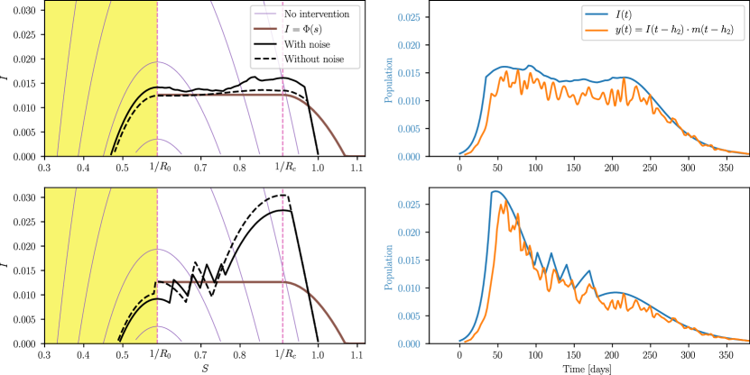
Figure 8: Closed-loop trajectories using the predictor (6) (top) and the observer (5) (bottom). Simulations were performed with and without measurement errors.

7 Conclusions

We have presented a predictor for systems with large input delays. The predictor is designed using the observer-predictor methodology introduced in the past years. In contrast with existing proposals, we present simple tuning criteria for ensuring the simultaneous stability of the polytopic model’s vertices. The stability of the complete polytopic model is then established formally with the help of a Lyapunov-Krasovskii functional. The functional can also be used to assess the sensitivity of the predictor with respect to error measurements. It is worthy of mentioning that it can also be used to find estimates of the domain of attraction, robustness bounds for the delay, and parameter uncertainties, among other problems of interest.

Our current research concerns the extension of the present results, obtained for two-dimensional systems, to $n$-dimensional ones, and to apply them to the study of more elaborated epidemic models involving states such as vaccinated individuals and asymptomatic ones.

References

• [1] Marco Tulio Angulo, Fernando Castaños, Jorge X. Velasco-Hernandez, and Jaime A. Moreno. A simple criterion to design optimal nonpharmaceutical interventions for epidemic outbreaks. medRxiv, 2020.
• [2] Zvi Artstein. Linear systems with delayed controls: a reduction. IEEE Transactions on Automatic control, 27(4):869–879, 1982.
• [3] R. E. Bellman and K. L. Cooke. Differential-difference equations. Academic Press, New York, 1963.
• [4] Stephen Boyd, Laurent El Ghaoui, Eric Feron, and Venkataramanan Balakrishnan. Linear Matrix Inequalities in System and Control Theory. Society for Industrial and Applied Mathematics, Philadelphia, 1994.
• [5] Marcos A. Capistran, Antonio Capella, and J. Andres Christen. Forecasting hospital demand during covid-19 pandemic outbreaks, 2020. arXiv.
• [6] E. Estrada-Sánchez, M. Velasco-Villa, and H. Rodríguez-Cortés. Prediction-based control for nonlinear systems with input delay. Mathematical Problems in Engineering, 2017.
• [7] I. Estrada-Sánchez, M. Velasco-Villa, and H. Rodríguez-Cortés. prediction based control for nonlinear systems with input delay. Mathematical Problems in Engineering, (October):Article ID 7415418, 2017.
• [8] Emilia Fridman. Introduction to Time-Delay Systems, Analysis and Control. Birkhäuser, 2014.
• [9] Keqin Gu, Jie Chen, and Vladimir L Kharitonov. Stability of time-delay systems. Springer Science & Business Media, 2003.
• [10] Yong He, Min Wu, Jin-Hua She, and Guo-Ping Liu. Parameter-dependent lyapunov functional for stability of time-delay systems with polytopic-type uncertainties. IEEE Transactions on Automatic control, 49(5):828–832, 2004.
• [11] Iasson Karafyllis and Miroslav Krstic. Stabilization of nonlinear delay systems using approximate predictors and high-gain observers. Automatica, 49(12):3623 – 3631, 2013.
• [12] Hasan K. Khalil. Nonlinear Systems. Prentice-Hall, Upper Saddle River, New Jersey, 1996.
• [13] Vladimir L Kharitonov. Predictor-based controls: the implementation problem. Differential Equations, 51(13):1675–1682, 2015.
• [14] Miroslav Krstic and Andrey Smyshlyaev. Boundary control of PDEs: A course on backstepping designs, volume 16. Siam, 2008.
• [15] V. Lechappe, E. Moulay, and F. Plestan. Prediction-based control for lti systems with uncertain time-varying delays and partial state knowledge. International Journal of Control, 91(6):1403–1414, 2018.
• [16] Andrzej Manitius and A Olbrot. Finite spectrum assignment problem for systems with delays. IEEE Transactions on Automatic Control, 24(4):541–552, 1979.
• [17] Wim Michiels and Silviu-Iulian Niculescu. Stability and Stabilization of Time-Delay Systems. Society for Industrial and Applied Mathematics, 2007.
• [18] Sabine Mondié and Wim Michiels. Finite spectrum assignment of unstable time-delay systems with a safe implementation. IEEE Transactions on Automatic Control, 48(12):2207–2212, 2003.
• [19] Majdeddin Najafi, Saeed Hosseinnia, Farid Sheikholeslam, and Mohammad Karimadini. Closed-loop control of dead time systems via sequential sub-predictors. International Journal of Control, 86(4):599–609, 2013.
• [20] J. Neimark. D-subdivisions and spaces of quasipolynomials. Prikl., Mat. Meh, 13:349–380, 1949.
• [21] B. O’Donoghue, E. Chu, N. Parikh, and S. Boyd. Conic optimization via operator splitting and homogeneous self-dual embedding. Journal of Optimization Theory and Applications, 169(3):1042–1068, June 2016.
• [22] Oluwaseun Sharomi and Tufail Malik. Optimal control in epidemiology. Annals of Operations Research, 251:55–71, 2017.
• [23] Otto JM Smith. A controller to overcome dead time. ISA J., 6:28–33, 1959.
• [24] Bin Zhou, Zongli Lin, and Guang-Ren Duan. Truncated predictor feedback for linear systems with long time-varying input delays. Automatica, 48(10):2387–2399, 2012.
• [25] Bin Zhou, Qingsong Liu, and Frédéric Mazenc. Stabilization of linear systems with both input and state delays by observer-predictors. Automatica, 83:368–377, 2017.