Adaptive Extra-Gradient Methods
for Min-Max Optimization and Games

Abstract.

We present a new family of min-max optimization algorithms that automatically exploits the geometry of the gradient data observed at earlier iterations to perform more informative extra-gradient steps in later ones. Thanks to this adaptation mechanism, the proposed methods automatically detect whether the problem is smooth or not, without requiring any prior tuning by the optimizer. As a result, the algorithm simultaneously achieves order-optimal convergence rates, i.e., it converges to an $\varepsilon$-optimal solution within $\operatorname{\mathcal{O}}(1/\varepsilon)$ iterations in smooth problems, and within $\operatorname{\mathcal{O}}(1/\varepsilon^{2})$ iterations in non-smooth ones. Importantly, these guarantees do not require any of the standard boundedness or Lipschitz continuity conditions that are typically assumed in the literature; in particular, they apply even to problems with singularities (such as resource allocation problems and the like). This adaptation is achieved through the use of a geometric apparatus based on Finsler metrics and a suitably chosen mirror-prox template that allows us to derive sharp convergence rates for the methods at hand.

1. Introduction

The surge of recent breakthroughs in generative adversarial networks [21], robust reinforcement learning [45], and other adversarial learning models [30] has sparked renewed interest in the theory of min-max optimization problems and games. In this broad setting, it has become empirically clear that, ceteris paribus, the simultaneous training of two (or more) antagonistic models faces drastically new challenges relative to the training of a single one. Perhaps the most prominent of these challenges is the appearance of cycles and recurrent (or even chaotic) behavior in min-max games. This has been studied extensively in the context of learning in bilinear games, in both continuous [44, 34, 17] and discrete time [13, 35, 20, 19], and the methods proposed to overcome recurrence typically focus on mitigating the rotational component of min-max games.

The method with the richest history in this context is the extra-gradient (EG) algorithm of Korpelevich [26] and its variants. The extra-gradient (EG) algorithm exploits the Lipschitz smoothness of the problem and, if coupled with a Polyak–Ruppert averaging scheme, it achieves an $\operatorname{\mathcal{O}}(1/T)$ rate of convergence in smooth, convex-concave min-max problems [38]. This rate is known to be tight [37, 43] but, in order to achieve it, the original method requires the problem’s Lipschitz constant to be known in advance. If the problem is not Lipschitz smooth (or the algorithm is run with a vanishing step-size schedule), the method’s rate of convergence drops to $\operatorname{\mathcal{O}}(1/\sqrt{T})$.

Our contributions.

Our aim in this paper is to provide an algorithm that automatically adapts to smooth / non-smooth min-max problems and games, and achieves order-optimal rates in both classes without requiring any prior tuning by the optimizer. In this regard, we propose a flexible algorithmic scheme, which we call AdaProx, and which exploits gradient data observed at earlier iterations to perform more informative extra-gradient steps in later ones. Thanks to this mechanism, and to the best of our knowledge, AdaProx is the first algorithm that simultaneously achieves the following:

1. An $\operatorname{\mathcal{O}}\big{(}1/\sqrt{T}\big{)}$ convergence rate in non-smooth problems and $\operatorname{\mathcal{O}}(1/T)$ in smooth ones.

2. Applicability to min-max problems and games where the standard boundedness / Lipschitz continuity conditions required in the literature do not hold.

3. Convergence without prior knowledge of the problem’s parameters (e.g., whether the problem’s defining vector field is smooth or not, its smoothness modulus if it is, etc.).

Our proposed method achieves the above by fusing the following ingredients: itn) a family of local norms – a Finsler metric – capturing any singularities in the problem at hand; itn) a suitable mirror-prox template; and itn) an adaptive step-size policy in the spirit of Rakhlin & Sridharan [48]. We also show that, under a suitable coherence assumption, the sequence of iterates generated by the algorithm converges, thus providing an appealing alternative to iterate averaging in cases where the method’s “last iterate” is more appropriate (for instance, if using AdaProx to solve non-monotone problems).

Related work.

There have been several works improving on the guarantees of the original extra-gradient/mirror-prox template. We review the most relevant of these works below; for convenience, we also tabulate these contributions in Table 1. Because many of these works appear in the literature on variational inequalities [16], we also use this language in the sequel.

In unconstrained problems with an operator that is locally Lipschitz continuous (but not necessarily globally so), the golden ratio algorithm (GRAAL) [32] achieves convergence without requiring prior knowledge of the problem’s Lipschitz parameter. However, golden ratio algorithm (GRAAL) provides no rate guarantees for non-smooth problems – and hence, a fortiori, no interpolation guarantees either. By contrast, such guarantees are provided in problems with a bounded domain by the generalized mirror-prox (GMP) algorithm of Stonyakin et al. [52] under the umbrella of Hölder continuity. Still, nothing is known about the convergence of GRAAL /  generalized mirror-prox (GMP) in problems with singularities (i.e., when the problem’s defining vector field blows up at a boundary point of the problem’s domain).

Another method that simultaneously achieves an $\operatorname{\mathcal{O}}(1/\sqrt{T})$ rate in non-smooth problems and an $\operatorname{\mathcal{O}}(1/T)$ rate in smooth ones is the recent algorithm of Bach & Levy [2]. The Bach–Levy (BL) algorithm employs an adaptive, AdaGrad-like step-size policy which allows the method to interpolate between the two regimes – and this, even with noisy gradient feedback. On the negative side, the BL algorithm requires a bounded domain with a (Bregman) diameter that is known in advance; as a result, its theoretical guarantees do not apply to problems with an unbounded domain. In addition, the BL algorithm makes crucial use of operator boundedness and Lipschitz continuity; extending the BL method beyond this standard framework is a highly non-trivial endeavor which formed a big part of this paper’s motivation.

Operators with singularities were treated in a recent series of papers [1, 18, 53] by means of a “Bregman continuity” or “Lipschitz-like” condition in the spirit of Bauschke et al. [4] and Lu et al. [29]. Albeit different, the adaptive methods presented in [1, 18] are both order-optimal in the smooth case, without requiring any knowledge of the problem’s smoothness modulus. On the other hand, like GRAAL – but unlike GMP – they do not provide any rate interpolation guarantees between smooth and non-smooth problems. Finally, the method of [53] provides an “inexact model” framework that unifies the approach of [18] and [52], providing rate interpolation in the Hölder case and convergence in problems with singularities; however, in problems with an unbounded domain, it still requires an initial guess of a compact set containing a solution.

	EG [26, 38]	GRAAL [32]	GMP [52]	AMP [1, 18]	BL [2]	AdaProx [ours]
Param. Agnostic	✗	✓	Partial	✓	Partial	✓
Rate Interpolation	✗	✗	✓	✗	✓	✓
Unb. Domain	✗	✓	✗	✗	✗	✓
Singularities	✗	✗	✗	✓	✗	✓

Table 1. Overview of related work. For the purposes of this table, “parameter-agnostic” means that the method does not require prior knowledge of the parameters of the problem it was designed to solve (Lipschitz modulus, domain diameter, etc.); “rate interpolation” means that the algorithm’s convergence rate is $\operatorname{\mathcal{O}}(1/T)$ or $\operatorname{\mathcal{O}}\big{(}1/\sqrt{T}\big{)}$ in smooth / non-smooth problems respectively; “unbounded domain” is self-explanatory; and, finally, “singularities” means that the problem’s defining vector field may blow up at a boundary point of the problem’s domain.

2. Problem Setup and Blanket Assumptions

We begin in this section by reviewing some basics for min-max problems and games.

2.1. Min-max / Saddle-point problems

A min-max game is a saddle-point problem of the form

$$\min_{\theta\in\Theta}\max_{\phi\in\Phi}\mathcal{L}(\theta,\phi)$$ (SP)

where $\Theta$, $\Phi$ are convex subsets of some ambient real space and $\mathcal{L}\colon\Theta\times\Phi\to\mathbb{R}$ is the problem’s loss function. In the game-theoretic interpretation of (SP), the player controlling $\theta$ seeks to minimize $\mathcal{L}(\theta,\phi)$ for any value of the maximization variable $\phi$, while the player controlling $\phi$ seeks to maximize $\mathcal{L}(\theta,\phi)$ for any value of the minimization variable $\theta$. Accordingly, solving (SP) consists of finding a Nash equilibrium (NE), i.e., an action profile $(\theta^{\ast},\phi^{\ast})\in\Theta\times\Phi$ such that

$$\mathcal{L}(\theta^{\ast},\phi)\leq\mathcal{L}(\theta^{\ast},\phi^{\ast})\leq\mathcal{L}(\theta,\phi^{\ast})\quad\text{for all $\theta\in\Theta$, $\phi\in\Phi$}.$$ (1)

By the minimax theorem of von Neumann [54], Nash equilibria are guaranteed to exist when $\Theta,\Phi$ are compact and $\mathcal{L}$ is convex-concave (i.e., convex in $\theta$ and concave in $\phi$). Much of our paper is motivated by the question of calculating a Nash equilibrium $(\theta^{\ast},\phi^{\ast})$ of (SP) in the context of von Neumann’s theorem; we expand on this below.

2.2. Games

Going beyond the min-max setting, a continuous game in normal form is defined as follows: First, consider a finite set of players $\mathcal{N}=\{1,\dotsc,N\}$, each with their own action space $\mathcal{K}_{i}\in\mathbb{R}^{d_{i}}$ (assumed convex but possibly not closed). During play, each player selects an action $x_{i}$ from $\mathcal{K}_{i}$ with the aim of minimizing a loss determined by the ensemble $x\coloneqq(x_{i};x_{-i})\coloneqq(x_{1},\dotsc,x_{N})$ of all players’ actions. In more detail, writing $\mathcal{K}\coloneqq\prod_{i}\mathcal{K}_{i}$ for the game’s total action space, we assume that the loss incurred by the $i$-th player is $\ell_{i}(x_{i};x_{-i})$, where $\ell_{i}\colon\mathcal{K}\to\mathbb{R}$ is the player’s loss function.

In this context, a Nash equilibrium is any action profile $x^{\ast}\in\mathcal{K}$ that is unilaterally stable, i.e.,

$$\ell_{i}(x^{\ast}_{i};x^{\ast}_{-i})\leq\ell_{i}(x_{i};x^{\ast}_{-i})\quad\text{for all $x_{i}\in\mathcal{K}_{i}$ and all $i\in\mathcal{N}$}.$$ (NE)

If each $\mathcal{K}_{i}$ is compact and $\ell_{i}$ is convex in $x_{i}$, existence of Nash equilibria is guaranteed by the theorem of Debreu [14]. Given that a min-max problem can be seen as a two-player zero-sum game with $\ell_{1}=\mathcal{L}$, $\ell_{2}=-\mathcal{L}$, von Neumann’s theorem may in turn be seen as a special case of Debreu’s; in the sequel, we describe a first-order characterization of Nash equilibria that encapsulates both.

In most cases of interest, the players’ loss functions are individually subdifferentiable on a subset $\mathcal{X}$ of $\mathcal{K}$ with $\operatorname{ri}\mathcal{K}\subseteq\mathcal{X}\subseteq\mathcal{K}$ [49, 22]. This means that there exists a (possibly discontinuous) vector field $V_{i}\colon\mathcal{X}\to\mathbb{R}^{d_{i}}$ such that

$$\ell_{i}(x^{\prime}_{i};x_{-i})\geq\ell_{i}(x_{i};x_{-i})+\langle V_{i}(x),x^{\prime}_{i}-x_{i}\rangle$$ (2)

for all $x\in\mathcal{X}$, $x^{\prime}\in\mathcal{K}$ and all $i\in\mathcal{N}$ [22]. In the simplest case, if $\ell_{i}$ is differentiable at $x$, then $V_{i}(x)$ can be interpreted as the gradient of $\ell_{i}$ with respect to $x_{i}$. The raison d’être of the more general definition (2) is that it allows us to treat non-smooth loss functions that are common in machine learning (such as $L^{1}$-regularized losses). We make this distinction precise below:

1. If there is no continuous vector field $V_{i}(x)$ satisfying (2), the game is called non-smooth.

2. If there is a continuous vector field $V_{i}(x)$ satisfying (2), the game is called smooth.

Remark.

We stress here that the adjective “smooth” refers to the game itself: for instance, if $\ell(x)=\lvert x\rvert$ for $x\in\mathbb{R}$, the game is not smooth and any $V$ satisfying (2) is discontinuous at $0$. In this regard, the above boils down to whether the (individual) subdifferential of each $\ell_{i}$ admits a continuous selection.

2.3. Resource allocation and equilibrium problems

The notion of a Nash equilibrium captures the unilateral minimization of the players’ individual loss functions. In many pratical cases of interest, a notion of equilibrium is still relevant, even though it is not necessarily attached to the minimization of individual loss functions. Such problems are known as “equilibrium problems” [16, 27]; to avoid unnecessary generalities, we focus here on a relevant problem that arises in distributed computing architectures (such as GPU clusters and the like).

To state the problem, consider a distributed computing grid consisting of $N$ parallel processors that serve demands arriving at a rate of $\rho$ per unit of time (measured e.g., in flop/s). If the maximum processing rate of the $i$-th node is $\mu_{i}$ (without overclocking), and jobs are buffered and served on a first-come, first-served (FCFS) basis, the mean time required to process a unit demand at the $i$-th node is given by the Kleinrock M/M/1 response function $\tau_{i}(x_{i})=1/(\mu_{i}-x_{i})$, where $x_{i}$ denotes the node’s load [6]. Accordingly, the set of feasible loads that can be processed by the grid is $\mathcal{X}\coloneqq\{(x_{1},\dotsc,x_{N}):0\leq x_{i}<\mu_{i},x_{1}+\dotsm+x_{N}=\rho\}$.

In this context, a load profile $x^{\ast}\in\mathcal{X}$ is said to be balanced if no infinitesimal process can be better served by buffering it at a different node [42]; formally, this amounts to the so-called Wardrop equilibrium condition

$$\tau_{i}(x_{i}^{\ast})\leq\tau_{j}(x_{j}^{\ast})\quad\text{for all $i,j\in\mathcal{N}$ with $x^{\ast}_{i}>0$}.$$ (WE)

We note here a crucial difference between (WE) and (NE): if we view the grid’s computing nodes as “players”, the constraint $\sum_{i}x_{i}=\rho$ means that there is no allowable unilateral deviation $(x_{i}^{\ast};x_{-i}^{\ast})\mapsto(x_{i};x_{-i}^{\ast})$ with $x_{i}\neq x_{i}^{\ast}$. As a result, (NE) is meaningless as a requirement for this equilibrium problem.

As we discuss below, this resource allocation problem will require the full capacity of our framework.

2.4. Variational inequalities

Importantly, all of the above problems can be restated as a variational inequality of the form

$$\text{Find $x^{\ast}\in\mathcal{X}$ such that}\;\;\langle V(x^{\ast}),x-x^{\ast}\rangle\geq 0\;\;\text{for all $x\in\mathcal{X}$}.$$ (VI)

In the above, $\mathcal{X}$ is a convex subset of $\mathbb{R}^{d}$ (not necessarily closed) that represents the problem’s domain. The problem’s defining vector field $V\colon\mathcal{X}\to\mathbb{R}^{d}$ is then given as follows: In min-max problems and games, $V$ is any field satisfying (2); otherwise, in equilibrium problems of the form (WE), the components of $V$ are $V_{i}=\tau_{i}$ (we leave the details of this verification to the reader).

This equivalent formulation is quite common in the literature on min-max / equilibrium problems [16, 15, 33, 27], and it is often referred to as the “vector field formulation” [3, 9, 24]. Its usefulness lies in that it allows us to abstract away from the underlying game-theoretic complications (multiple indices, individual subdifferentials, etc.) and provides a unifying framework for a wide range of problems in machine learning, signal processing, operations research, and many other fields [16, 50]. For this reason, our analysis will focus almost exclusively on solving (VI), and we will treat $V$ and $\mathcal{X}\subseteq\mathbb{R}^{d}$, $d=\sum_{i}d_{i}$, as the problem’s primitive data.

2.5. Merit functions and monotonicity

A widely used assumption in the literature on equilibrium problems and variational inequalities is the monotonicity condition

$$\langle V(x)-V(x^{\prime}),x-x^{\prime}\rangle\geq 0\quad\text{for all $x,x^{\prime}\in\mathcal{X}$}.$$ (MC)

In single-player games, monotonicity is equivalent to convexity of the optimizer’s loss function; in min-max games, it is equivalent to $\mathcal{L}$ being convex-concave [27]; etc. In the absence of monotonicity, approximating an equilibrium is PPAD-hard [12], so we will state most of our results under (MC).

Now, to assess the quality of a candidate solution $\hat{x}\in\mathcal{X}$, we will employ the restricted merit function

$$\operatorname{Gap}_{\mathcal{C}}(\hat{x}) =\sup\nolimits_{x\in\mathcal{C}}\langle V(x),\hat{x}-x\rangle,$$ (3)

where the “test domain” $\mathcal{C}$ is a nonempty convex subset of $\mathcal{X}$ [40, 25, 16]. The motivation for this is provided by the following proposition:

Proposition 1.

Let $\mathcal{C}$ be a nonempty convex subset of $\mathcal{X}$. Then: itn) $\operatorname{Gap}_{\mathcal{C}}(\hat{x})\geq 0$whenever $\hat{x}\in\mathcal{C}$; and itn) if $\operatorname{Gap}_{\mathcal{C}}(\hat{x})=0$ and $\mathcal{C}$ contains a neighborhood of $\hat{x}$, then $\hat{x}$ is a solution of (VI).

Proposition 1 generalizes an earlier characterization by Nesterov [40] and justifies the use of $\operatorname{Gap}_{\mathcal{C}}(x)$ as a merit function for (VI); to streamline our presentation, we defer the proof to the paper’s supplement. Moreover, to avoid trivialities, we will also assume that the solution set $\mathcal{X}^{\ast}$ of (VI) is nonempty and we will reserve the notation $x^{\ast}$ for solutions of (VI). Together with monotonicity, this will be our only blanket assumption.

3. The Extra-Gradient Algorithm and its Limits

Perhaps the most widely used solution method for games and variational inequalities is the extra-gradient (EG) algorithm of Korpelevich [26] and its variants [47, 48, 31]. This algorithm has a rich history in optimization, and it has recently attracted considerable interest in the fields of machine learning and AI, see e.g., [13, 19, 35, 9, 23, 24, 36] and references therein.

In its simplest form, for problems with closed domains, the algorithm proceeds recursively as

$$X_{t+1/2}=\operatorname{\Pi}(X_{t}-\gamma_{t}V_{t}),\qquad X_{t+1}=\operatorname{\Pi}(X_{t}-\gamma_{t}V_{t+1/2}),$$ (EG)

where $\operatorname{\Pi}(x)=\operatorname*{arg\,min}_{x^{\prime}\in\mathcal{X}}\lVert x^{\prime}-x\rVert$ is the Euclidean projection on $\mathcal{X}$, $V_{t}\coloneqq V(X_{t})$ for $t=1,3/2,\dotsc$, and $\gamma_{t}>0$, is the method’s step-size. Then, running (EG) for $T$ iterations, the algorithm returns the “ergodic average”

$$\bar{X}_{T}=\frac{\sum_{t=1}^{T}\gamma_{t}X_{t+1/2}}{\sum_{t=1}^{T}\gamma_{t}}.$$ (4)

In this setting, the main guarantees for (EG) date back to [38] and can be summarized as follows:

1. For non-smooth problems (discontinuous $V$): Assume $V$ is bounded, i.e., there exists some $M>0$ such that

   $$\lVert V(x)\rVert\leq M\quad\text{for all $x\in\mathcal{X}$}.$$ (BD)

   Then, if (EG) is run with a step-size of the form $\gamma_{t}\propto 1/\sqrt{t}$, we have

   $$\operatorname{Gap}_{\mathcal{C}}(\bar{X}_{T})=\operatorname{\mathcal{O}}\big{(}1/\sqrt{T}\big{)}.$$ (5)

2. For smooth problems (continuous $V$): Assume $V$ is $L$-Lipschitz continuous, i.e.,

   $$\lVert V(x)-V(x^{\prime})\rVert\leq L\lVert x-x^{\prime}\rVert\quad\text{for all $x,x^{\prime}\in\mathcal{X}$}.$$ (LC)

   Then, if (EG) is run with a constant step-size $\gamma<1/L$, we have

   $$\operatorname{Gap}_{\mathcal{C}}(\bar{X}_{T})=\operatorname{\mathcal{O}}(1/T).$$ (6)

Remark.

In the above, $\lVert\cdot\rVert$ is tacitly assumed to be the standard Euclidean norm. Non-Euclidean considerations will play a crucial role in the sequel, but they are not necessary for the moment.

Importantly, the distinction between smooth and non-smooth problems cannot be lifted: the bounds (5) and (6) are tight in their respective problem classes and they cannot be improved without further assumptions [37, 43]. Moreover, we should also note the following:

1. The algorithm changes drastically from the non-smooth to the smooth case: non-smoothness requires $\gamma_{t}\propto 1/\sqrt{t}$, but such a step-size cannot achieve a fast $\operatorname{\mathcal{O}}(1/T)$ rate.

2. If (EG) is run with a constant step-size, $L$ must be known in advance; otherwise, running (EG) with an ill-adapted step-size ($\gamma>1/L)$ could lead to non-convergence.

We illustrate this failure of (EG) in Fig. 1. As we discussed in the introduction, our aim in the sequel will be to provide a single, adaptive algorithm that simultaneously achieves the following: itn) an order-optimal $\operatorname{\mathcal{O}}\big{(}1/\sqrt{T}\big{)}$ convergence rate in non-smooth problems and $\operatorname{\mathcal{O}}(1/T)$ in smooth ones; itn) convergence in problems where the boundedness / Lipschitz continuity conditions (BD) / (LC) no longer hold; and itn) achieves all this without prior knowledge of the problem’s parameters.

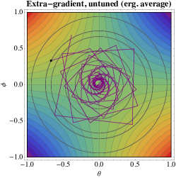
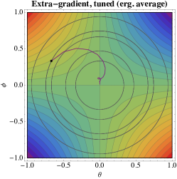
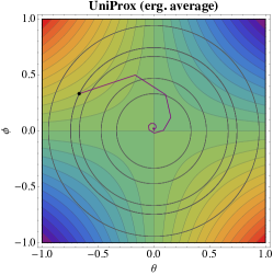
Figure 1. The behavior of (EG) in the bilinear min-max problem $\mathcal{L}(\theta,\phi)=\theta\phi$ with $\theta,\phi\in[-1,1]$. Given the clipping at $[-1,1]$, this problem is smooth with $L=1$; instead, in the unconstrained case, both (BD) and (LC) fail. Still, even in the constrained case, running (EG) with a step-size only slightly above the $1/L$ bound ($L=1$, $\gamma=1.04$) results in a dramatic convergence failure (left plot). Tuning the step-size of (EG) resolves this problem (center), but a constant step-size makes the algorithm unnecessarily conservative towards the end. The proposed AdaProx algorithm automatically exploits previous gradient data to perform more informative extra-gradient steps in later ones, thus achieving faster convergence without tuning.

4. Rate Interpolation: the Euclidean Case

As a prelude to our main result, we provide in this section an adaptive version of (EG) that achieves the “best of both worlds” in the Euclidean setting of Section 3, i.e., an $\operatorname{\mathcal{O}}\big{(}1/\sqrt{T}\big{)}$ convergence rate in problems satisfying (BD), and an $\operatorname{\mathcal{O}}(1/T)$ rate in problems satisfying (LC). Our starting point is the observation that, if the sequence $X_{t}$ produced by (EG) converges to a solution of (VI), the difference

$$\delta_{t}\coloneqq\lVert V_{t+1/2}-V_{t}\rVert=\lVert V(X_{t+1/2})-V(X_{t})\rVert$$ (7)

must itself become vanishingly small if $V$ is (Lipschitz) continuous. On the contrary, if $V$ is discontinuous, this difference may remain bounded away from zero (consider for example the $L^{1}$ loss $\ell(x)=\lvert x\rvert$ near $0$). Based on this observation, we consider the adaptive step-size policy:

$$\gamma_{t+1}=1\Big{/}\sqrt{1+\textstyle\sum_{s=1}^{t}\delta_{s}^{2}}.$$ (8)

The intuition behind (8) is as follows: If $V$ is not smooth and $\liminf_{t\to\infty}\delta_{t}>0$, then $\gamma_{t}$ will vanish at a $\Theta\big{(}1/\sqrt{t}\big{)}$ rate, which is the optimal step-size schedule for problems satisfying (BD) but not (LC). Instead, if $V$ satisfies (LC) and $X_{t}$ converges to a solution $x^{\ast}$ of (VI), it is plausible to expect that the infinite series $\sum_{t}\delta_{t}^{2}$ is summable, in which case the step-size $\gamma_{t}$ will not vanish as $t\to\infty$. Furthermore, since $\delta_{t}$ is defined in terms of successive gradient differences, it automatically exploits the variation of the gradient data observed up to time $t$, so it can be expected to adjust to the “local” Lipschitz constant of $V$ around a solution $x^{\ast}$ of (VI).

Our step-size policy and motivation are similar in spirit to the “predictable sequence” approach of [48]. color=DodgerBlue!20!LightGray,author=PM]Is this ok?
However, making our reasoning precise (especially the summability of $\sum_{t}\delta_{t}^{2}$ in the smooth case) involves considerable conceptual and technical difficulties that we present in detail in the supplement. For now, we only state (without proof) our main result for problems satisfying (BD) or (LC).

Theorem 1.

Suppose $V$ satisfies (MC), let $\mathcal{C}$ be a compact neighborhood of a solution of (VI), and let $0pt=\sup_{x\in\mathcal{C}}\lVert X_{1}-x\rVert^{2}$. If (EG) is run with the adaptive step-size policy (8), we have:

a) If $$V \operatorname{Gap}_{\mathcal{C}}(\bar{X}_{T})=\operatorname{\mathcal{O}}\left(\frac{0pt+4M^{3}+\log(1+4M^{2}T)}{\sqrt{T}}\right).\hskip 51.6665pt$$ satisfies (BD): (9a)

b) If $$V \operatorname{Gap}_{\mathcal{C}}(\bar{X}_{T})=\operatorname{\mathcal{O}}\left(0pt\big{/}T\right).$$ satisfies (LC): (9b)

Theorem 1 (which is proved in the sequel as a special case of Theorem 2) should be compared to the corresponding results of Bach & Levy [2]. In the non-smooth case, [2] provides a bound of the form $\tilde{\operatorname{\mathcal{O}}}(\alpha MD/\sqrt{T})$ with $D^{2}=\frac{1}{2}\max_{x\in\mathcal{X}}\lVert x\rVert^{2}-\frac{1}{2}\min_{x\in\mathcal{X}}\lVert x\rVert^{2}$ (recall that [2] only treats problems with a bounded domain), and $\alpha=\max\{M/M_{0},M_{0}/M\}$ where $M_{0}$ is an initial estimate of $M$. The worst-case value of $\alpha$ is $\operatorname{\mathcal{O}}(M)$ when good estimates are not readily available; in this regard, (9a) essentially replaces the $\operatorname{\mathcal{O}}(D)$ constant of Bach & Levy [2] by $\operatorname{\mathcal{O}}(M)$. Since $D=\infty$ in problems with an unbounded domain, Theorem 1 provides a significant improvement in this regard.

In terms of $L$, the smooth guarantee of Bach & Levy [2] is $\tilde{\operatorname{\mathcal{O}}}(\alpha^{2}LD^{2}/T)$, so the multiplicative constant in the bound also becomes infinite in problems with an unbounded domain. In our case, $D^{2}$ is replaced by $0pt$ (which is also finite) times an addiitional multiplicative constant which is increasing in $M$ and $L$ (but is otherwise asymptotic, so it is not included in the statement of Theorem 1). This removes an additional limitation in the results of Bach & Levy [2]; going beyond this improvement, in the next sections we drop even the Euclidean regularity requirements (BD)/(LC), and we provide a corresponding rate interpolation result that does not require either condition.

5. Finsler Regularity

To motivate our analysis outside the setting of (BD)/(LC), consider the vector field

$$V_{i}(x)=(\mu_{i}-x_{i})^{-1}+\lambda\operatorname{\mathds{1}}\{x_{i}>0\},\quad i=1,\dotsc,N,$$ (10)

which corresponds to the distributed computing problem of Section 2.3 plus a regularization term designed to limit the activation of computing nodes at low loads. Clearly, we have $\lVert V(x)\rVert\to\infty$ whenever $x_{i}\to 0^{+}$, so (BD) and (LC) both fail (the latter even if $\lambda=0$). On the other hand, if we consider the “local” norm $\lVert v\rVert_{x,\ast}=\sum_{i=1}^{d}(\mu_{i}-x_{i})\,\lvert v_{i}\rvert$, we have $\lVert V(x)\rVert_{x,\ast}\leq d+\lambda\sum_{i=1}^{d}\mu_{i}$, so $V$ is bounded relative to $\lVert\cdot\rVert_{x,\ast}$. This observation motivates the use of a local – as opposed to global – norm, which we define formally as follows:

Definition 1.

A Finsler metric on a convex subset $\mathcal{X}$ of $\mathbb{R}^{d}$ is a continuous function $F\colon\mathcal{X}\times\mathbb{R}^{d}\to\mathbb{R}_{+}$ which satisfies the following properties for all $x\in\mathcal{X}$ and all $z,z^{\prime}\in\mathbb{R}^{d}$:

1. Subadditivity: $F(x;z+z^{\prime})\leq F(x;z)+F(x;z^{\prime})$.

2. Absolute homogeneity: $F(x;\lambda z)=\lvert\lambda\rvert F(x;z)$ for all $\lambda\in\mathbb{R}$.

3. Positive-definiteness: $F(x;z)\geq 0$ with equality if and only if $z=0$.

Given a Finsler metric on $\mathcal{X}$, the induced primal / dual local norms on $\mathcal{X}$ are respectively defined as

$$\lVert z\rVert_{x}=F(x;z)\quad\text{and}\quad\lVert v\rVert_{x,\ast} =\max\{\langle v,z\rangle:F(x;z)=1\}$$ (11)

for all $x\in\mathcal{X}$ and all $z,v\in\mathbb{R}^{d}$. We will also say that a Finsler metric on $\mathcal{X}$ is regular when $\lVert v\rVert_{x^{\prime},\ast}/\lVert v\rVert_{x,\ast}=1+\operatorname{\mathcal{O}}(\lVert x^{\prime}-x\rVert_{x})$ for all $x,x^{\prime}\in\mathcal{X}$, $v\in\mathbb{R}^{d}$. Finally, for simplicity, we will also assume in the sequel that $\lVert\cdot\rVert_{x}\geq\nu\lVert\cdot\rVert$ for some $\nu>0$ and all $x\in\mathcal{X}$ (this last assumption is for convenience only, as the norm could be redefined to $\lVert\cdot\rVert_{x}\leftarrow\lVert\cdot\rVert_{x}+\nu\lVert\cdot\rVert$ without affecting our theoretical analysis).

When $\mathcal{X}$ is equipped with a regular Finsler metric as above, we will say that it is a Finsler space.

Example 5.1.

Let $F(x;z)=\lVert z\rVert$ where $\lVert\cdot\rVert$ denotes the reference norm of $\mathcal{X}=\mathbb{R}^{d}$. Then the properties of Definition 1 are satisfied trivially. $\blacktriangleleft$

Example 5.2.

For a more interesting example of a Finsler structure, consider the set $\mathcal{X}=(0,1]^{d}$ and the metric $\lVert z\rVert_{x}=\max_{i}\lvert z_{i}\rvert/x_{i}$, $z\in\mathbb{R}^{d}$, $x\in\mathcal{X}$. In this case $\lVert v\rVert_{x,\ast}=\sum_{i=1}^{d}x_{i}\lvert v_{i}\rvert$ for all $v\in\mathbb{R}^{d}$, and the only property of Definition 1 that remains to be proved is that of regularity. To that end, we have

$$\textstyle\lVert v\rVert_{x^{\prime},\ast}-\lVert v\rVert_{x,\ast}\leq\sum_{i=1}^{d}\lvert v_{i}\rvert\cdot\lvert x^{\prime}_{i}-x_{i}\rvert=\sum_{i=1}^{d}x_{i}\lvert v_{i}\rvert\cdot\lvert x^{\prime}_{i}-x_{i}\rvert/x_{i}\leq\lVert v\rVert_{x,\ast}\cdot\lVert x^{\prime}-x\rVert_{x}.$$ (12)

Hence, by dividing by $\lVert v\rVert_{x,\ast}$, we readily get $\lVert v\rVert_{x^{\prime},\ast}/\lVert v\rVert_{x,\ast}\leq 1+\lVert x-x^{\prime}\rVert_{x}$ i.e., $\lVert\cdot\rVert_{x}$ is regular in the sense of Definition 1. As we discuss in the sequel, this metric plays an important role for distributed computing problems of the form presented in Section 2.3. $\blacktriangleleft$

With all this in hand, we will say that a vector field $V\colon\mathcal{X}\to\mathbb{R}^{d}$ is

1. Metrically bounded if there exists some $M>0$ such that

   $$\lVert V(x)\rVert_{x,\ast}\leq M\quad\text{for all $x\in\mathcal{X}$}.$$ (MB)

2. Metrically smooth if there exists some $L>0$ such that

   $$\lVert V(x^{\prime})-V(x)\rVert_{x,\ast}\leq L\lVert x^{\prime}-x\rVert_{x^{\prime}}\quad\text{for all $x^{\prime},x\in\mathcal{X}$}.$$ (MS)

The notion of metric boundedness/smoothness extends that of ordinary boundedness/Lipschitz continuity to a Finsler context; note also that, even though neither side of (MS) is unilaterally symmetric under the change $x\leftrightarrow x^{\prime}$, the condition (MS) as a whole is. Our next example shows that this extension is proper, i.e., (BD)/(LC) may both fail while (MB)/(MS) both hold:

Example 5.3.

Consider the change of variables $x_{i}\rightsquigarrow 1-x_{i}/\mu_{i}$ in the resource allocation problem of Section 2.3. Then, writing $V_{i}(x)=-(1/x_{i})-\lambda\operatorname{\mathds{1}}\{x_{i}<1\}$ for the transformed field (10) under this change of variables, we readily get $V_{i}(x)\to-\infty$ as $x_{i}\to 0^{+}$; as a result, both (BD) and (LC) fail to hold for any global norm on $\mathbb{R}^{d}$. Instead, under the local norm $\lVert z\rVert_{x}=\max_{i}\lvert z\rvert_{i}/x_{i}$, we have:

1. For all $\lambda\geq 0$, $V$ satisfies (MB) with $M=d(1+\lambda)$: $\lVert V(x)\rVert_{x,\ast}\leq\sum_{i=1}^{d}x_{i}\cdot(1/x_{i}+\lambda)=d(1+\lambda)$.

2. For $\lambda=0$, $V$ satisfies (MS) with $L=d$: indeed, for all $x,x^{\prime}\in\mathcal{X}$, we have

   $$\lVert V(x^{\prime})-V(x)\rVert_{x,\ast}=\sum\nolimits_{i=1}^{d}x_{i}\left\lvert\frac{1}{x^{\prime}_{i}}-\frac{1}{x_{i}}\right\rvert=\sum\nolimits_{i=1}^{d}\frac{\lvert x^{\prime}_{i}-x_{i}\rvert}{x^{\prime}_{i}}\leq d\max\nolimits_{i}\frac{\lvert x^{\prime}_{i}-x_{i}\rvert}{x^{\prime}_{i}}=d\lVert x^{\prime}-x\rVert_{x^{\prime}}.$$ (13)

6. The AdaProx Algorithm and its Guarantees

The method.

We are now in a position to define a family of algorithms that is capable of interpolating between the optimal smooth/non-smooth convergence rates for solving (VI) without requiring either (BD) or (LC). To do so, the key steps in our approach will be to (it n) equip $\mathcal{X}$ with a suitable Finsler structure (as in Section 5); and (it n) replace the Euclidean projection in (EG) with a suitable “Bregman proximal” step that is compatible with the chosen Finsler structure on $\mathcal{X}$.

We begin with the latter (assuming that $\mathcal{X}$ is equipped with an arbitrary Finsler structure):

Definition 2.

We say that $h:\mathbb{R}^{d}\to\mathbb{R}\cup\{\infty\}$ is a Bregman-Finsler function on $\mathcal{X}$ if:

1. $h$ is convex, lower semi-continuous (l.s.c.), $\operatorname{cl}(\operatorname{dom}h)=\operatorname{cl}(\mathcal{X})$, and $\operatorname{dom}\partial h=\mathcal{X}$.

2. The subdifferential of $h$ admits a continuous selection $\nabla h(x)\in\partial h(x)$ for all $x\in\mathcal{X}$.

3. $h$ is strongly convex, i.e., there exists some $K>0$ such that

   $$h(x^{\prime})\geq h(x)+\langle\nabla h(x),x^{\prime}-x\rangle+\tfrac{K}{2}\lVert x^{\prime}-x\rVert^{2}_{x}$$ (14)

   for all $x\in\mathcal{X}$ and all $x^{\prime}\in\operatorname{dom}h$.

The Bregman divergence induced by $h$ is defined for all $x\in\mathcal{X}$, $x^{\prime}\in\operatorname{dom}h$ as

$$D(x^{\prime},x)=h(x^{\prime})-h(x)-\langle\nabla h(x),x^{\prime}-x\rangle$$ (15)

and the associated prox-mapping is defined for all $x\in\mathcal{X}$ and $y\in\mathbb{R}^{d}$ as

$$P_{x}(y)=\operatorname*{arg\,min}\nolimits_{x^{\prime}\in\mathcal{X}}\{\langle y,x-x^{\prime}\rangle+D(x^{\prime},x)\}.$$ (16)

Definition 2 is fairly technical, so some clarifications are in order. First, to connect this definition with the Euclidean setup of Section 4, the prox-mapping (16) should be seen as the Bregman equivalent of a Euclidean projection step, i.e., $\operatorname{\Pi}(x+y)\leftrightsquigarrow P_{x}(y)$. Second, a key difference between Definition 2 and other definitions of Bregman functions in the literature [7, 10, 5, 25, 39, 40, 51, 8] is that $h$ is assumed strongly convex relative to a local norm – not a global norm. This “locality” will play a crucial role in allowing the proposed methods to adapt to the geometry of the problem. For concreteness, we provide below an example that expands further on Examples 5.2 and 5.3:

Example 6.1.

Consider the local norm $\lVert z\rVert_{x}=\max_{i}\lvert z_{i}\rvert/x_{i}$ on $\mathcal{X}=(0,1]^{d}$ and let $h(x)=\sum_{i=1}^{d}1/x_{i}$ on $(0,1]^{d}$. We then have

$$D(x^{\prime},x)=\sum_{i=1}^{d}\bigg{[}\frac{1}{x^{\prime}_{i}}-\frac{1}{x_{i}}+\frac{x^{\prime}_{i}-x_{i}}{x_{i}^{2}}\bigg{]}=\sum_{i=1}^{d}\frac{(x^{\prime}_{i}-x_{i})^{2}}{x_{i}^{2}x^{\prime}_{i}}\geq\sum_{i=1}^{d}(1-x^{\prime}_{i}/x_{i})^{2}\geq\lVert x^{\prime}-x\rVert^{2}_{x}$$ (17)

i.e., $h$ is $1$-strongly convex relative to $\lVert\cdot\rVert_{x}$ on $\mathcal{X}$. $\blacktriangleleft$

With all this is in place, the extra-gradient method can be adapted to our current setting as follows:

$$X_{t+1/2} =P_{X_{t}}(-\gamma_{t}V_{t}) \qquad\delta_{t} =\lVert V_{t+1/2}-V_{t}\rVert_{X_{t+1/2},\ast}$$ (AdaProx)

$$X_{t+1} =P_{X_{t}}(-\gamma_{t}V_{t+1/2}) \qquad\gamma_{t+1} =1\Big{/}\sqrt{1+\textstyle\sum_{s=1}^{t}\delta_{s}^{2}}$$

with $V_{t}=V(X_{t})$, $t=1,3/2,\dotsc$, as in Section 3. In words, this method builds on the template of (EG) by (it n) replacing the Euclidean projection with a mirror step; (it n) replacing the global norm in (8) with a dual Finsler norm evaluated at the algorithm’s leading state $X_{t+1/2}$. The first of these two steps is the main ingredient of the mirror-prox (MP) algorithm of Nemirovski [38]; the name “AdaProx” has beeen chosen precisely because the proposed method can be seen as a mirror-prox method that adapts between the smooth and non-smooth regimes.

Convergence speed.

With all this in hand, our main result for AdaProx can be stated as follows:

Theorem 2.

Suppose $V$ satisfies (MC), let $\mathcal{C}$ be a compact neighborhood of a solution of (VI), and set $0pt=\sup_{x\in\mathcal{C}}D(x,X_{1})$ Then, the AdaProx algorithm enjoys the guarantees:

a) If $$V \operatorname{Gap}_{\mathcal{C}}(\bar{X}_{T})=\operatorname{\mathcal{O}}\left(\frac{0pt+M^{3}(1+1/K)^{2}+\log(1+4M^{2}(1+2/K)^{2}T)}{\sqrt{T}}\right).$$ satisfies (MB): (18a)

b) If $$V \operatorname{Gap}_{\mathcal{C}}(\bar{X}_{T})=\operatorname{\mathcal{O}}\left(0pt\big{/}T\right).$$ satisfies (MS): (18b)

For the constants that appear in Eq. 18, we refer the reader to the discussion following Theorem 1 (of course, since Theorem 1 is a special case of Theorem 2, it is not surprising that the same remarks apply). As for the proof of Theorem 2, it is quite intricate, so we defer it to the paper’s supplement. We only mention here that its key element is the determination of the asymptotic behavior of the adaptive step-size policy $\gamma_{t}$ in the non-smooth and smooth regimes, i.e., under (MB) and (MS) respectively. At a very high level, (MB) guarantees that the difference sequence $\delta_{t}$ is bounded, which implies in turn that $\sum_{t=1}^{T}\gamma_{t}=\Omega(\sqrt{T})$ and eventually yields the bound (18a) for the algorithm’s ergodic average $\bar{X}_{T}$. On the other hand, if (MS) kicks in, we have the following finer result:

Lemma 1.

Assume $V$ satisfies (MS). Then, itn) $\gamma_{t}$decreases monotonically to a strictly positive limit $\gamma_{\infty}=\lim_{t\to\infty}\gamma_{t}>0$; and itn) the sequence $\delta_{t}$ is square summable: in particular, $\sum_{t=1}^{\infty}\delta_{t}^{2}=1/\gamma_{\infty}^{2}-1$.

By means of this lemma (which we prove in the paper’s supplement), it follows that $\sum_{t=1}^{T}\gamma_{t}\geq\gamma_{\infty}T=\Omega(T)$. Because the algorithm’s rate of convergence is controlled by this quantity, it ultimately follows that AdaProx enjoys an $\operatorname{\mathcal{O}}(1/T)$ rate of convergence under (MS). However, the details of the ensuing calculations are quite complicated, so we defer them to the supplement.

Trajectory convergence.

In complement to Theorem 2, we also provide a trajectory convergence result that governs the actual iterates of the AdaProx algorithm:

Theorem 3.

Suppose that $\langle V(x),x-x^{\ast}\rangle<0$ whenever $x^{\ast}$ is a solution of (VI) and $x$ is not. If, in addition, $V$ satisfies (MB) or $\eqref{eq:MS}$, the iterates $X_{t}$ of AdaProx converge to a solution of (VI).

The importance of this result is that, in many practical applications (especially in non-monotone problems), it is more common to harvest the “last iterate” of the method ($X_{t}$) rather than its ergodic average ($\bar{X}_{T}$); as such, Theorem 3 provides a certain justification for this design choice.

The proof of Theorem 3 relies on non-standard arguments, so we relegate it to the supplement. Structurally, the first step is to show that $X_{t}$ visits any neighborhood of a solution point $x^{\ast}\in\mathcal{X}^{\ast}$ infinitely often (this is where the coherence assumption $\langle V(x),x-x^{\ast}\rangle$ is used). The second is to use this trapping property in conjunction with a suitable “energy inequality” to establish convergence via the use of a quasi-Fejér technique as in [11]; this part is detailed in a separate appendix.

7. Numerical Experiments

We conclude in this section with a numerical illustration of the convergence properties of AdaProx in two different settings: itn) bilinear min-max games; and itn) a simple Wasserstein GAN in the spirit of Daskalakis et al. [13] with the aim of learning an unknown covariance matrix.

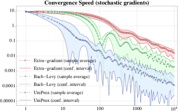
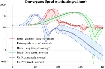
Figure 2. Numerical comparison between the extra-gradient (EG), Bach–Levy (BL) and AdaProx algorithms (red circles, green squares and blue triangles respectively). The figure on the left shows the methods’ convergence in a $100\times 100$ bilinear game; the one on the right shows the methods’ convergence in a non-convex/non-concave covariance learning problem. In both cases, the parameters of the EG and BL algorithms have been tuned with a grid search (AdaProx has no parameters to tune). All curves have been averaged over $S=100$ sample runs, and the $95\%$ confidence interval is indicated by the shaded area.

Bilinear min-max games.

For our first set of experiments, we consider a min-max game of the form of the form $\mathcal{L}(\theta,\phi)=(\theta-\theta^{\ast})^{\top}A(\phi-\phi^{\ast})$ with $\theta,\phi\in\mathbb{R}^{100}$ and $A\in\mathbb{R}^{100}\times\mathbb{R}^{100}$ (drawn i.i.d. component-wise from a standard Gaussian). To test the convergence of AdaProx beyond the “full gradient” framework, we ran the algorithm with stochastic gradient signals of the form $V_{t}=V(X_{t})+U_{t}$ where $U_{t}$ is drawn i.i.d. from a centered Gaussian distribution with unit covariance matrix. We then plotted in Fig. 2 the squared gradient norm $\lVert V(\bar{X}_{T})\rVert^{2}$ of the method’s ergodic average $\bar{X}_{T}$ after $T$ iterations (so values closer to zero are better). For benchmarking purposes, we also ran the extra-gradient (EG) and Bach–Levy (BL) algorithms [2] with the same random seed for the simulated gradient noise. The step-size parameter of the EG algorithm was chosen as $\gamma_{t}=0.025/\sqrt{t}$, whereas the BL algorithm was run with diameter and gradient bound estimation parameters $D_{0}=.5$ and $M_{0}=2.5$ respectively (both determined after a hyper-parameter search since the only theoretically allowable values are $D_{0}=M_{0}=\infty$; interestingly, very large values for $D_{0}$ and $M_{0}$ did not yield good results). The experiment was repeated $S=100$ times, and AdaProx gave consistently faster rates.

Covariance matrix learning.

Going a step further, we also considered the covariance learning game

$$\mathcal{L}(\theta,\phi)=\operatorname{\mathbb{E}}_{x\sim\mathcal{N}(0,\Sigma)}[x^{\top}\theta x]-\operatorname{\mathbb{E}}_{z\sim\mathcal{N}(0,I)}[z^{\top}\theta^{\top}\phi\theta z],\qquad\theta,\phi\in\mathbb{R}^{d}\times\mathbb{R}^{d}.$$ (19)

The goal here is to generate data drawn from a centered Gaussian distribution with unknown covariance $\Sigma$; in particular, this model follows the Wasserstein GAN formulation of Daskalakis et al. [13] with generator and discriminator respectively given by $G(z)=\theta z$ and $D(x)=x^{\top}\phi x$ (no clipping). For the experiments, we took $d=100$, a mini-batch of $m=128$ samples per update, and we ran the EG, BL and AdaProx algorithms as above, tracing the square norm of $V$ as a measure of convergence. Since the problem is non-monotone, there are several disjoint equilibrium components so the algorithms’ behavior is considerably more erratic; however, after this initial warm-up phase, AdaProx again gave the faster convergence rates.

Appendix A Properties of the restricted gap function

In this appendix, we discuss the basic properites of the restricted merit function $\operatorname{Gap}_{\mathcal{C}}$ introduced in (3). For completeness, we provide the proof of Proposition 1,which itself is an extension of a similar result by Nesterov [40]:

Proof of Proposition 1.

Let $x^{\ast}\in\mathcal{X}$ be a solution of (VI) so $\langle V(x^{\ast}),x-x^{\ast}\rangle\geq 0$ for all $x\in\mathcal{X}$. Then, by monotonicity, we get:

$$\langle V(x),x^{\ast}-x\rangle \leq\langle V(x)-V(x^{\ast}),x^{\ast}-x\rangle+\langle V(x^{\ast}),x^{\ast}-x\rangle$$

$$=-\langle V(x^{\ast})-V(x),x^{\ast}-x\rangle-\langle V(x^{\ast}),x-x^{\ast}\rangle\leq 0,$$ (A.1)

so $\operatorname{Gap}_{\mathcal{C}}(x^{\ast})\leq 0$. On the other hand, if $x^{\ast}\in\mathcal{C}$, we also get $\operatorname{Gap}(x^{\ast})\geq\langle V(x^{\ast}),x^{\ast}-x^{\ast}\rangle=0$, so we conclude that $\operatorname{Gap}_{\mathcal{C}}(x^{\ast})=0$.

For the converse statement, assume that $\operatorname{Gap}_{\mathcal{C}}(\hat{x})=0$ for some $\hat{x}\in\mathcal{C}$ and suppose that $\mathcal{C}$ contains a neighborhood of $\hat{x}$ in $\mathcal{X}$. First, we claim that the following inequality holds:

$$\langle V(x),x-\hat{x}\rangle\geq 0\quad\text{for all $x\in\mathcal{C}$}.$$ (A.2)

Indeed, assume to the contrary that there exists some $x_{1}\in\mathcal{C}$ such that

$$\langle V(x_{1}),x_{1}-\hat{x}\rangle<0.$$ (A.3)

This would then give

$$0=\operatorname{Gap}_{\mathcal{C}}(\hat{x})\geq\langle V(x_{1}),\hat{x}-x_{1}\rangle>0,$$ (A.4)

which is a contradiction. Now, we further claim that $\hat{x}$ is a solution of (VI),i.e.,:

$$\langle V(\hat{x}),x-\hat{x}\rangle\geq 0 x\in\mathcal{X}$$ for all . (A.5)

If we suppose that there exists some $z_{1}\in\mathcal{X}$ such that $\langle V(\hat{x}),z_{1}-\hat{x}\rangle<0$, then, by the continuity of $V$, there exists a neighborhood $U^{\prime}$ of $\hat{x}$ in $\mathcal{X}$ such that

$$\langle V(x),z_{1}-x\rangle<0\quad\text{for all $x\in U^{\prime}$}.$$ (A.6)

Hence, assuming without loss of generality that $U^{\prime}\subset U\subset\mathcal{C}$ (the latter assumption due to the assumption that $\mathcal{C}$ contains a neighborhood of $\hat{x}$), and taking $\lambda>0$ sufficiently small so that $x=\hat{x}+\lambda(z_{1}-\hat{x})\in U^{\prime}$, we get that $\langle V(x),x-\hat{x}\rangle=\lambda\langle V(x),z_{1}-\hat{x}\rangle<0$, in contradiction to (A.2). We conclude that $\hat{x}$ is a solution of (VI), as claimed. ∎

Appendix B Properties of Bregman functions and proximal mappings

In this appendix, we present some basic facts about Bregman functions and proximal mappings. Similar results exist in the literature in different contexts (see e.g., [40, 41, 25] and references therein), but given that many of our results rely on the use of local – as opposed to global – norms, we provide here complete statements and proofs. We then have the following basic lemma connecting the above notions:

Lemma B.1.

Let $h$ be a Bregman function on $\mathcal{X}$. Then, for all $p\in\operatorname{dom}h$, $x\in\operatorname{dom}\partial h$ and all $y\in\partial h(x)$, we have

$$\langle\nabla h(x),x-p\rangle\leq\langle y,x-p\rangle.$$ (B.1)

Proof.

By a simple continuity argument, it is sufficient to show that the inequality holds for the relative interior $\operatorname{ri}\mathcal{X}$ of $\mathcal{X}$. In order to show this, pick a base point $p\in\operatorname{ri}\mathcal{X}$, and let

$$\phi(t)=h(x+t(p-x))-[h(x)+\langle y,t(p-x)\rangle]\quad\text{for all $t\in[0,1]$}.$$ (B.2)

Since, $h$ is strongly convex and $y\in\partial h(x)$ due to the first equivalence, it follows that $\phi(t)\geq 0$ with equality if and only if $t=0$. Since, $\psi(t)=\langle\nabla h(x+t(p-x))-y,p-x\rangle$ is a continuous selection of subgradients of $\phi$ and both $\phi$ and $\psi$ are continuous over $[0,1]$, it follows that $\phi$ is continuously differentiable with $\phi^{\prime}=\psi$ on $[0,1]$. Hence, with $\phi$ convex and $\phi(t)\geq 0=\phi(0)$ for all $t\in[0,1]$, we conclude that $\phi^{\prime}(0)=\langle\nabla h(x)-y,p-x\rangle\geq 0$ and thus we obtain the result. ∎

The basic ingredient for establishing connections in the Bregman framework is a generalization of the rule of cosines which is known in the literature as the “three-point identity” [10] and will be the main tool for deriving the main estimations for our analysis. Being more precise, we have the following lemma:

Lemma B.2.

Let $h$ be a Bregman function on $\mathcal{X}$. Then, for all $p\in\mathcal{X}$ and all $x,x^{\prime}\in\mathcal{X}^{\circ}$, we have:

$$D(p,x^{\prime})=D(p,x)+D(x,x^{\prime})+\langle\nabla h(x^{\prime})-\nabla h(x),x-p\rangle$$ (B.3)

The proof of this lemma follows as in the classic Bregman case [10] so we omit it and proceed to derive some key bounds for the Bregman divergence before and after a mirror step:

Proposition B.1.

Let $h$ be a local Bregman function with strong convexity modulus $K>0$. Fix some $p\in\mathcal{X}$ and let $x^{+}=P_{x}(v)$ for some $x\in\mathcal{X}^{\circ}$ and $v\in\mathbb{R}^{d}$. We then have:

$$D(p,x^{+})\leq D(p,x)-D(x^{+},x)+\langle v,x^{+}-p\rangle$$ (B.4)

Proof.

By the three-point identity established in Lemma B.2, we get:

$$D(p,x)=D(p,x^{+})+D(x^{+},x)+\langle\nabla h(x)-\nabla h(x^{+}),x^{+}-p\rangle$$ (B.5)

By rearranging the terms we get:

$$D(p,x^{+})=D(p,x)-D(x^{+},x)+\langle\nabla h(x^{+})-\nabla h(x),x^{+}-p\rangle$$ (B.6)

Due to (B.1) and the fact that $x^{+}=P_{x}(v)$ so $\nabla h(x)+v\in\partial h(x^{+})$, we get the result. ∎

Thanks to the above estimations, we obtain the following inequalities relating the Bregman divergence between two prox-steps:

Proposition B.2.

Let $h$ be a Bregman function compatible on $\mathcal{X}$. Letting $x^{+}_{1}=P_{x}(v_{1})$ and $x^{+}_{2}=P_{x}(v_{2})$, we have:

$$D(p,x^{+}_{2}) \leq D(p,x)+\langle v_{2},x^{+}_{1}-p\rangle+[\langle v_{2},x^{+}_{2}-x^{+}_{1}\rangle-D(x^{+}_{2},x)]$$ (B.7a)

$$\leq D(p,x)+\langle v_{2},x^{+}_{1}-p\rangle+\langle v_{2}-v_{1},x^{+}_{2}-x^{+}_{1}\rangle-D(x^{+}_{2},x^{+}_{1})-D(x^{+}_{1},x).$$ (B.7b)

Proof.

For the first inequality, by applying Proposition B.1 for $x^{+}_{2}=P_{x}(v_{2})$, we get:

$$D(p,x^{+}_{2}) \leq D(p,x)-D(x^{+}_{2},x)+\langle v_{2},x^{+}_{2}-p\rangle$$

$$=D(p,x)+\langle v_{2},x^{+}_{1}-p\rangle+[\langle v_{2},x^{+}_{2}-x^{+}_{1}\rangle-D(x^{+}_{2},x)]$$ (B.8)

For the second inequality, we need to bound $\langle v_{2},x^{+}_{2}-x^{+}_{1}\rangle-D_{h}(x^{+}_{2},x)$. In particular, applying again Proposition B.1 for $p=x^{+}_{2}$, we get:

$$D(x^{+}_{2},x^{+}_{1})\leq D(x^{+}_{2},x)+\langle v_{1},x^{+}_{1}-x^{+}_{2}\rangle-D(x^{+}_{1},x)$$ (B.9)

and hence:

$$D(x^{+}_{2},x)\geq D(x^{+}_{2},x^{+}_{1})+D(x^{+}_{1},x)-\langle v_{1},x^{+}_{1}-x^{+}_{2}\rangle.$$ (B.10)

So, combining the above inequalities we get:

$$\langle v_{2},x^{+}_{2}-x^{+}_{1}\rangle-D(x^{+}_{2},x)\leq\langle v_{2},x^{+}_{2}-x^{+}_{1}\rangle-D(x^{+}_{2},x^{+}_{1})-D(x^{+}_{1},x)-\langle v_{1},x^{+}_{2}-x^{+}_{1}\rangle$$ (B.11)

and thus we get the second inequality as well. ∎

Appendix C Main bounds and energy inequality

In this appendix, we shall provide the bound of the variation of the operators, i.e.,

$$\lVert V(X_{t+1/2})-V(X_{t})\rVert^{2}_{X_{t},\ast}$$ (C.1)

that lies in the core of our analysis. To begin with, we recall that $(\mathcal{X},\lVert\cdot\rVert_{x})$ is a regular Finsler space, i.e., $\lVert v\rVert_{x,\ast}/\lVert v\rVert_{x^{\prime},\ast}=1+\operatorname{\mathcal{O}}(\lVert x-x^{\prime}\rVert_{x})$. However, in what follows we shall assume the more general condition:

$$\lVert v\rVert_{x,\ast}/\lVert v\rVert_{x^{\prime},\ast}\leq 1+\beta\left[\lVert x-x^{\prime}\rVert_{x}+\lVert x-x^{\prime}\rVert_{x^{\prime}}\right] \beta>0$$ for some (C.2)

Remark 1.

It is straightforward for one to observe that a regular Finsler space satisfies (C.2) for $\beta=1$.

Owning this regularity geometrical property for the problem’s domain we shall proceed into showing that

$$\lVert V(X_{t+1/2})-V(X_{t})\rVert^{2}_{X_{t},\ast}$$ (C.3)

is uniformly bounded. More precisely, we have the following lemma.

Lemma C.1.

Suppose that $V$ satisfies (MB). Then, the sequence $\lVert V(X_{t+1/2})-V(X_{t})\rVert^{2}_{X_{t},\ast}$ is bounded. In particular, the following inequality holds:

$$\lVert V(X_{t+1/2})-V(X_{t})\rVert^{2}_{X_{t},\ast}\leq C^{2}$$ (C.4)

with $C=2M+\beta\frac{4M}{K}$.

Proof.

It suffices to show that: $\lVert V(X_{t+1/2})-V(X_{t})\rVert_{X_{t+1/2},\ast}$ is bounded. More precisely, by the triangle inequality we have:

$$\lVert V(X_{t+1/2})-V(X_{t})\rVert_{X_{t+1/2},\ast}\leq\lVert V(X_{t+1/2})\rVert_{X_{t+1/2},\ast}+\lVert V(X_{t})\rVert_{X_{t+1/2},\ast}$$ (C.5)

Let us now bound the (RHS) part of (C.5) term by term. In particular, we have:

• For the first term $\lVert V(X_{t+1/2})\rVert_{X_{t+1/2},\ast}$ we readily get due to (MB):

  $$\lVert V(X_{t+1/2})\rVert_{X_{t+1/2},\ast}\leq M$$ (C.6)

• For the second term $\lVert V(X_{t})\rVert_{X_{t+1/2},\ast}$, we have:

  $$\lVert V(X_{t})\rVert_{X_{t+1/2},\ast}\leq\lVert V(X_{t})\rVert_{X_{t},\ast}+\beta\left[\lVert X_{t}-X_{t+1/2}\rVert_{X_{t}}+\lVert X_{t}-X_{t+1/2}\rVert_{X_{t+1/2}}\right]\\ \leq M+\beta\left[\lVert X_{t}-X_{t+1/2}\rVert_{X_{t}}+\lVert X_{t}-X_{t+1/2}\rVert_{X_{t+1/2}}\right]$$ (C.7)

  Therefore, it suffices to show that the quantity $\lVert X_{t}-X_{t+1/2}\rVert_{X_{t}}+\lVert X_{t}-X_{t+1/2}\rVert_{X_{t+1/2}}$ is bounded from above. Indeed, we have:

  $$D(X_{t},X_{t+1/2})+D(X_{t+1/2},X_{t}) =\langle\nabla h(X_{t})-\nabla h(X_{t+1/2}),X_{t}-X_{t+1/2}\rangle$$

  $$\leq\gamma_{t}\langle V(X_{t}),X_{t}-X_{t+1/2}\rangle$$

  $$\leq M\gamma_{t}\lVert X_{t}-X_{t+1/2}\rVert_{X_{t}}$$

  where the last inequality is obtained due to (MB). Moreover, due to (14) we get:

  $$D(X_{t},X_{t+1/2})+D(X_{t+1/2},X_{t}) \leq\gamma_{t}M\sqrt{\frac{2}{K}D(X_{t+1/2},X_{t})}$$

  $$\leq M\sqrt{\frac{2}{K}\left[D(X_{t},X_{t+1/2})+D(X_{t+1/2},X_{t})\right]}$$

  which yields

  $$D(X_{t},X_{t+1/2})+D(X_{t},X_{t+1/2})\leq\frac{2M^{2}}{K}$$ (C.8)

  Hence, due to the local strong convexity (14) of $h$, we get:

  $$\frac{K}{2}\left[\lVert X_{t}-X_{t+1/2}\rVert_{X_{t}}^{2}+\lVert X_{t}-X_{t+1/2}\rVert_{X_{t+1/2}}^{2}\right]\leq\frac{2M^{2}}{K}$$ (C.9)

  which in turn implies that:

  $$\lVert X_{t}-X_{t+1/2}\rVert_{X_{t}}\leq\frac{2M}{K} \lVert X_{t}-X_{t+1/2}\rVert_{X_{t+1/2}}\leq\frac{2M}{K}$$ and (C.10)

  and so,

  $$\lVert X_{t}-X_{t+1/2}\rVert_{X_{t}}+\lVert X_{t}-X_{t+1/2}\rVert_{X_{t+1/2}}\leq\frac{4M}{K}$$ (C.11)

  Moreover, by combining (C.7) and (C.11) we get:

  $$\lVert V(X_{t})\rVert_{X_{t+1/2},\ast}\leq M+\beta\frac{4M}{K}$$ (C.12)

Summarizing, (C.5) combined with (C.7) and (C.12) yields:

$$\lVert V(X_{t+1/2})-V(X_{t})\rVert_{X_{t+1/2},\ast}\leq 2M+\beta\frac{4M}{K}$$ (C.13)

and hence the result follows. ∎

We now proceed to prove the energy inequality stated in Lemma C.2.

Lemma C.2.

For all $x\in\mathcal{X}$, the iterates $X_{t}$ of AdaProx satisfy the recursive bound:

$$D(x,X_{t+1})\leq D(x,X_{t})-\gamma_{t}\langle V(X_{t+1/2}),X_{t+1/2}-x\rangle+\gamma_{t}\langle V(X_{t+1/2})-V(X_{t}),X_{t+1}-X_{t+1/2}\rangle\\ -D(X_{t+1},X_{t+1/2})-D(X_{t+1/2},X_{t})$$ (C.14)

Proof.

The result follows directly by setting $X_{1}^{+}=X_{t+1/2}$, $X_{2}^{+}=X_{t+1}$, $x=X_{t}$, $v_{1}=-\gamma_{t}V(X_{t})$ and $v_{2}=-\gamma_{t}V(X_{t+1/2})$ in Proposition B.2. ∎

Appendix D Rate interpolation guarantees

In this appendix, we provide the proof of the the regime-agnostic rate interpolation guarantees of the UniProx. In order, to provide the necessary the respective rates we shall provide an intermediate result concerning the case of (MS). Formally, we have the following lemma.

Lemma D.1.

Assume $V$ satisfies (MS) and $X_{t},X_{t+1/2}$ are the iterates of AdaProx. Then, the following hold:

1. $\gamma_{t}\to\inf_{t\in\mathbb{N}}\gamma_{t}=\gamma_{\infty}>0$

2. The sequence $\lVert V(X_{t+1/2})-V(X_{t})\rVert^{2}_{X_{t+1/2},\ast}$ is summable. In particular, we have:

   $$\sum_{t=1}^{+\infty}\lVert V(X_{t+1/2})-V(X_{t})\rVert^{2}_{X_{t+1/2},\ast}=\frac{1}{\gamma_{\infty}^{2}}-1$$ (D.1)

Proof.

Since $\gamma_{t}$ is decreasing and bounded from below ($\gamma_{t}\geq 0$), then we readily obtain that its limit exists and more precisely we have:

$$\lim_{t\to+\infty}\gamma_{t}=\inf_{t\in\mathbb{N}}\gamma_{t}=\gamma_{\infty}\geq 0$$ (D.2)

Let us now assume that $\gamma_{\infty}=0$. Then, by recalling (C.14):

$$D(p,X_{t+1})\leq D(p,X_{t})-\gamma_{t}\langle V(X_{t+1/2}),X_{t+1/2}-p\rangle+\gamma_{t}\langle V(X_{t+1/2})-V(X_{t}),X_{t+1}-X_{t+1/2}\rangle\\ -D(X_{t+1/2},X_{t})-D(X_{t+1},X_{t+1/2})$$ (D.3)

By rearranging the above and telescoping $t=1,\dotsc,T$ we get:

$$\sum_{t=1}^{T}\gamma_{t}\langle V(X_{t+1/2}),X_{t+1/2}-p\rangle\leq D(p,X_{1})+\sum_{t=1}^{T}\gamma_{t}\langle V(X_{t+1/2})-V(X_{t}),X_{t+1}-X_{t+1/2}\rangle\\ -\sum_{t=1}^{T}D(X_{t+1/2},X_{t})-\sum_{t=1}^{T}D(X_{t+1},X_{t+1/2})$$ (D.4)

whereas, by applying Fenchel-Young inequality to the above we readily get:

$$\sum_{t=1}^{T}\gamma_{t}\langle V(X_{t+1/2}),X_{t+1/2}-p\rangle\leq D(p,X_{1})+\frac{1}{2K}\sum_{t=1}^{T}\gamma_{t}^{2}\lVert V(X_{t+1/2})-V(X_{t})\rVert^{2}_{X_{t+1/2},\ast}\\ +\frac{K}{2}\sum_{t=1}^{T}\lVert X_{t+1}-X_{t+1/2}\rVert_{X_{t+1/2}}^{2}-\sum_{t=1}^{T}D(X_{t+1/2},X_{t})-\sum_{t=1}^{T}D(X_{t+1},X_{t+1/2})$$ (D.5)

and by considering that by (14):

$$\frac{K}{2}\sum_{t=1}^{T}\lVert X_{t+1}-X_{t+1/2}\rVert^{2}_{X_{t+1/2}}-\sum_{t=1}^{T}D(X_{t+1},X_{t+1/2})\leq 0$$ (D.6)

we finally obtain:

$$\sum_{t=1}^{T}\gamma_{t}\langle V(X_{t+1/2}),X_{t+1/2}-p\rangle\leq D(p,X_{1})+\frac{1}{2K}\sum_{t=1}^{T}\gamma_{t}^{2}\lVert V(X_{t+1/2})-V(X_{t})\rVert^{2}_{X_{t+1/2},\ast}\\ -\sum_{t=1}^{T}D(X_{t+1/2},X_{t})$$ (D.7)

Therefore, by the definition (MS) we have:

$$\sum_{t=1}^{T}\gamma_{t}\langle V(X_{t+1/2}),X_{t+1/2}-p\rangle\leq D(p,X_{1})+\frac{1}{2K}\sum_{t=1}^{T}\gamma_{t}^{2}\lVert V(X_{t+1/2})-V(X_{t})\rVert^{2}_{X_{t+1/2},\ast}\\ -\frac{K}{2L^{2}}\sum_{t=1}^{T}\lVert V(X_{t+1/2})-V(X_{t})\rVert_{X_{t+1/2},\ast}^{2}$$ (D.8)

which becomes:

$$\sum_{t=1}^{T}\gamma_{t}\langle V(X_{t+1/2}),X_{t+1/2}-p\rangle\leq D(p,X_{1})+\sum_{t=1}^{T}\left[\frac{\gamma_{t}^{2}}{2K}-\frac{K}{4L^{2}}\right]\lVert V(X_{t+1/2})-V(X_{t})\rVert^{2}_{X_{t+1/2},\ast}\\ -\frac{K}{4L^{2}}\sum_{t=1}^{T}\lVert V(X_{t+1/2})-V(X_{t})\rVert_{X_{t+1/2},\ast}^{2}$$ (D.9)

Now, by setting $p=x^{\ast}$ with $x^{\ast}$ being a solution of (VI) and using the fact that $\langle V(X_{t+1/2}),X_{t+1/2}-x^{\ast}\rangle\geq 0$ and $D(x^{\ast},X_{1})\leq D^{\prime}$ (by the compatibility of $h$), we obtain:

$$\frac{K}{4L^{2}}\sum_{t=1}^{T}\lVert V(X_{t+1/2})-V(X_{t})\rVert^{2}_{X_{t+1/2},\ast}\leq D^{\prime}+\sum_{t=1}^{T}\left[\frac{\gamma_{t}^{2}}{2K}-\frac{K}{4L^{2}}\right]\lVert V(X_{t+1/2})-V(X_{t})\rVert^{2}_{X_{t+1/2},\ast}$$ (D.10)

Moreover, by observing that the quantity $\left[\frac{\gamma_{t}^{2}}{2K}-\frac{K}{4L^{2}}\right]\leq 0$, whenever $\gamma_{t}\leq\sqrt{2}K/2L$ and since we assumed that $\gamma_{t}\to 0$, there exists some $t_{0}\in\mathbb{N}$ such that:

$$\left[\frac{\gamma_{t}^{2}}{2K}-\frac{K}{4L^{2}}\right]\leq 0\;\;\text{for all}\;\;t\geq t_{0}$$ (D.11)

Therefore, (D.10) becomes:

$$\frac{1}{\gamma_{T+1}}-1=\sum_{t=1}^{T}\lVert V(X_{t+1/2})-V(X_{t})\rVert^{2}_{X_{t+1/2},\ast}\leq D^{\prime}+\sum_{t=1}^{t_{0}}\left[\frac{\gamma_{t}^{2}}{2K}-\frac{K}{4L^{2}}\right]\lVert V(X_{t+1/2})-V(X_{t})\rVert^{2}_{X_{t+1/2},\ast}$$ (D.12)

In addition, since $1/\gamma_{T+1}\to+\infty$, by the fact that $\gamma_{t}\to 0$, this yields that:

$$+\infty\leq D^{\prime}+\sum_{t=1}^{t_{0}}\left[\frac{\gamma_{t}^{2}}{2K}-\frac{K}{4L^{2}}\right]\lVert V(X_{t+1/2})-V(X_{t})\rVert^{2}_{X_{t+1/2},\ast}$$ (D.13)

which is a contradiction. Hence, we get that:

$$\lim_{t\to+\infty}\gamma_{t}=\inf_{t\in\mathbb{N}}\gamma_{t}=\gamma_{\infty}>0$$ (D.14)

In order to prove our second claim, we first recall the definition of $\gamma_{t}$:

$$\gamma_{t}=\frac{1}{\sqrt{1+\sum_{j=1}^{t-1}\lVert V(X_{t+1/2})-V(X_{t})\rVert_{X_{t+1/2,\ast}}^{2}}}$$ (D.15)

whereas by developing and rearranging we have:

$$\sum_{j=1}^{t-1}\lVert V(X_{t+1/2})-V(X_{t})\rVert_{X_{t+1/2,\ast}}^{2}=\frac{1}{\gamma_{t}^{2}}-1$$ (D.16)

Hence, by taking limits on both sides we get:

$$\sum_{t=1}^{+\infty}\lVert V(X_{t+1/2})-V(X_{t})\rVert_{X_{t+1/2,\ast}}^{2}=\lim_{t\to+\infty}\sum_{j=1}^{t-1}\lVert V(X_{t+1/2})-V(X_{t})\rVert_{X_{t+1/2,\ast}}^{2}=\frac{1}{\gamma_{\infty}^{2}}-1$$ (D.17)

where $0\leq\frac{1}{\gamma_{\infty}^{2}}-1<+\infty$, since $0<\gamma_{\infty}\leq 1$ and therefore the result follows. ∎

Proof of Theorem 2.

By recalling (C.14) we have:

$$D(p,X_{t+1})\leq D(p,X_{t})-\gamma_{t}\langle V(X_{t+1/2}),X_{t+1/2}-p\rangle+\gamma_{t}\langle V(X_{t+1/2})-V(X_{t}),X_{t+1}-X_{t+1/2}\rangle\\ -D(X_{t+1/2},X_{t})-D(X_{t+1},X_{t+1/2})$$ (D.18)

We start our analysis rearranging (C.14). In particular, by telescoping $t=1,\dotsc,T$ we get:

$$\sum_{t=1}^{T}\gamma_{t}\langle V(X_{t+1/2}),X_{t+1/2}-p\rangle\leq D(p,X_{1})+\sum_{t=1}^{T}\gamma_{t}\langle V(X_{t+1/2})-V(X_{t}),X_{t+1}-X_{t+1/2}\rangle\\ -\sum_{t=1}^{T}D(X_{t+1/2},X_{t})-\sum_{t=1}^{T}D(X_{t+1},X_{t+1/2})$$ (D.19)

On the other hand, since $V$ is monotone, we readily get:

$$\gamma_{t}\langle V(p),X_{t+1/2}-p\rangle\leq\gamma_{t}\langle V(X_{t+1/2}),X_{t+1/2}-p\rangle$$ (D.20)

Thus, combining (D.20) and (D.19), dividing by $\sum_{t=1}^{T}\gamma_{t}$ and setting $\bar{X}_{T}=\left[\sum_{t=1}^{T}\gamma_{t}\right]^{-1}\sum_{t=1}^{T}\gamma_{t}X_{t+1/2}$ we get:

$$\langle V(p),\bar{X}_{T}-p\rangle\leq D(p,X_{1})+\sum_{t=1}^{T}\gamma_{t}\langle V(X_{t+1/2})-V(X_{t}),X_{t+1}-X_{t+1/2}\rangle-\sum_{t=1}^{T}D(X_{t+1/2},X_{t})\\ -\sum_{t=1}^{T}D(X_{t+1},X_{t+1/2})$$ (D.21)

whereas, by applying Fenchel-Young inequality to the above we readily get:

$$\langle V(p),\bar{X}_{T}-p\rangle\leq D(p,X_{1})+\frac{1}{2K}\sum_{t=1}^{T}\gamma_{t}^{2}\lVert V(X_{t+1/2})-V(X_{t})\rVert^{2}_{X_{t+1/2},\ast}+\frac{K}{2}\sum_{t=1}^{T}\lVert X_{t+1}-X_{t+1/2}\rVert_{X_{t+1/2}}^{2}\\ -\sum_{t=1}^{T}D(X_{t+1/2},X_{t})-\sum_{t=1}^{T}D(X_{t+1},X_{t+1/2})$$ (D.22)

Thus, if $\mathcal{C}$ is a compact neighbourhood of the solution set $\mathcal{X}^{\ast}$, considering that by (14):

$$\frac{K}{2}\sum_{t=1}^{T}\lVert X_{t+1}-X_{t+1/2}\rVert^{2}_{X_{t+1/2}}-\sum_{t=1}^{T}D(X_{t+1},X_{t+1/2})\leq 0$$ (D.23)

and taking suprema on both sides, yields:

$$\operatorname{Gap}_{\mathcal{C}}(\bar{X}_{T})\leq\left[\sum_{t=1}^{T}\gamma_{t}\right]^{-1}(\sup_{p\in\mathcal{C}}D(p,X_{1})+\frac{1}{2K}\sum_{t=1}^{T}\gamma_{t}^{2}\lVert V(X_{t+1/2})-V(X_{t})\rVert^{2}_{X_{t+1/2},\ast}\\ -\sum_{t=1}^{T}D(X_{t+1/2},X_{t}))$$ (D.24)

Case 1: Convergence under (MB).

Therefore, in order to determine the convergence speed of $\overline{X}_{T}$ under (MB), we shall examine the asymptotic behaviour of each term of the nominator on the (RHS) of (D.31). In particular, we have the following:

• For the first term: we readily get by the compactness of $\mathcal{C}$,

  $$\sup_{p\in\mathcal{C}}D(p,X_{1})\leq D^{\prime} D^{\prime}>0$$ for some constant . (D.25)

  by the compatibility of the regularizer $h$.

• For the second term: $\sum_{t=1}^{T}\gamma_{t}^{2}\lVert V(X_{t+1/2})-V(X_{t})\rVert_{X_{t+1/2}}^{2}$, we have:

  $$\sum_{t=1}^{T}\gamma_{t}^{2}\lVert V(X_{t+1/2})-V(X_{t})\rVert_{X_{t+1/2}}^{2}=\sum_{t=1}^{T}(\gamma_{t}^{2}-\gamma_{t+1}^{2})\lVert V(X_{t+1/2})-V(X_{t})\rVert_{X_{t+1/2}}^{2}\\ +\sum_{t=1}^{T}\gamma_{t+1}^{2}\lVert V(X_{t+1/2})-V(X_{t})\rVert_{X_{t+1/2}}^{2}$$ (D.26)

  Hence, $\gamma_{t}$ is non-increasing and therefore $(\gamma_{t}^{2}-\gamma_{t+1}^{2}\geq 0)$, and $\gamma_{t}\leq 1$ the above becomes:

  $$\sum_{t=1}^{T}\gamma_{t}^{2}\lVert V(X_{t+1/2})-V(X_{t})\rVert_{X_{t+1/2}}^{2} \leq C^{2}+\sum_{t=1}^{T}\gamma_{t+1}\lVert V(X_{t+1/2})-V(X_{t})\rVert_{X_{t+1/2}}^{2}$$

  $$\leq C^{2}+\sum_{t=1}^{T}\frac{\lVert V(X_{t+1/2})-V(X_{t})\rVert_{X_{t+1/2}}^{2}}{1+\sum_{j=1}^{t}\lVert V(X_{t+1/2})-V(X_{t})\rVert_{X_{t+1/2}}^{2}}$$

  $$\leq C^{2}+1+\log(1+\sum_{t=1}^{T}\lVert V(X_{t+1/2})-V(X_{t})\rVert_{X_{t+1/2}}^{2})$$

  with the last inequality being obtained by Lemma F.1 which combined with (MB) yields:

  $$\sum_{t=1}^{T}\gamma_{t}^{2}\lVert V(X_{t+1/2})-V(X_{t})\rVert_{X_{t+1/2}}^{2}\leq C^{2}+1+\log(1+C^{2}T)$$ (D.27)

Finally, for $\sum_{t=1}^{T}\gamma_{t}$, we have the following upper-bound

$$\sum_{t=1}^{T}\gamma_{t}=\sum_{t=1}^{T}\frac{1}{\sqrt{1+\sum_{j=1}^{t-1}\lVert V(X_{t+1/2})-V(X_{t})\rVert_{X_{t+1/2,\ast}}^{2}}}\geq\sum_{t=1}^{T}\frac{1}{\sqrt{1+tC^{2}}}$$ (D.28)

which yields:

$$\sum_{t=1}^{T}\gamma_{t}=\Omega(\sqrt{T})\;\;\text{and}\;\;\sum_{t=1}^{T}\gamma_{t}\to+\infty$$ (D.29)

Now, by combining (D.25), (D.27) and (D.29) we readily get that under (MB) we get that:

$$\operatorname{Gap}_{\mathcal{C}}(\bar{X}_{T})=\operatorname{\mathcal{O}}(1/\sqrt{T}).$$ (D.30)

Case 2: Convergence under (MS).

We now suppose that $V$ satisfies (MS) condition. By applying Lemma D.1 along with :

$$\sum_{t=1}^{T}\gamma_{t}\langle V(X_{t+1/2}),X_{t+1/2}-p\rangle\leq D(p,X_{1})+\frac{1}{2K}\sum_{t=1}^{T}\gamma_{t}^{2}\lVert V(X_{t+1/2})-V(X_{t})\rVert^{2}_{X_{t+1/2},\ast}\\ -\sum_{t=1}^{T}D(X_{t+1/2},X_{t})$$ (D.31)

by examining the asymptotic behaviour term by term, we get:

• For the first term $D(x^{\ast},X_{1})$, since $x^{\ast}\in\operatorname{dom}V=\operatorname{dom}h$ and $X_{1}\in\operatorname{dom}\partial h$, we have:

  $$D(x^{\ast},X_{1})<+\infty$$ (D.32)

• For the second term $\sum_{t=1}^{T}\gamma_{t}^{2}\lVert V(X_{t+1/2})-V(X_{t})\rVert_{X_{t+1/2},\ast}^{2}$we have:

  $$\sum_{t=1}^{T}\gamma_{t}^{2}\lVert V(X_{t+1/2})-V(X_{t})\rVert_{X_{t+1/2},\ast}^{2}\leq\sum_{t=1}^{T}\lVert V(X_{t+1/2})-V(X_{t})\rVert_{X_{t+1/2},\ast}^{2}$$ (D.33)

  and by applying Lemma D.1 we have:

  $$\sum_{t=1}^{T}\gamma_{t}^{2}\lVert V(X_{t+1/2})-V(X_{t})\rVert_{X_{t+1/2},\ast}^{2}\leq\frac{1}{\gamma_{\infty}^{2}}-1$$ (D.34)

  with $\gamma_{\infty}=\inf_{t}\gamma_{t}>0$.

Finally, by applying Lemma D.1 once more by considering $\gamma_{\infty}=\inf_{t\in\mathbb{N}}\gamma_{t}>0$ we have:

$$\sum_{t=1}^{T}\gamma_{t}\geq\gamma_{\infty}\sum_{t=1}^{T}1=\gamma_{\infty}T$$ (D.35)

which yields:

$$\sum_{t=1}^{T}\gamma_{t}=\Omega(T)$$ (D.36)

and the result follows. ∎

Appendix E Last iterate’s convergence analysis

In this appendix, we establish the convergence of the sequence generated by (AdaProx), i.e., its so-called last iterate. In particular, we show that the actual iterates (before averaging) of AdaProx converge towards the solution set $\mathcal{X}^{\ast}$.This result comprises of two parts: first we extract convergent subsequences of $X_{t},X_{t+1/2}$ to the said set; then we apply the "trapping" argument described in Section 6 .

Lemma E.1.

Suppose that $V$ satisfies (MB) (respectively (MS)) and $X_{t},X_{t+1/2}$ are the iterates of AdaProx. Then, the following hold:

1. $\lVert X_{t+1/2}-X_{t}\rVert\to 0$ while $t\to+\infty$

2. $\max\{D(X_{t+1/2},X_{t}),D(X_{t},X_{t+1/2})\}\leq\frac{2M^{2}}{K}\gamma_{t}^{2}$

Proof.

For the proof of the first claim, we shall treat the cases of (MB) and (MS) individually.

Case 1: Under (MB) condition.

Since $\gamma_{t}$ is decreasing and bounded from below, then we readily obtain that. its limit exists and more precisely:

$$\lim_{t\to+\infty}\gamma_{t}=\gamma_{\infty}\geq 0$$ (E.1)

We shall distinguish two individual cases:

• $\gamma_{\infty}>0$: By recalling the definition of the adaptive step-size:

  $$\gamma_{t}=\frac{1}{\sqrt{1+\sum_{j=1}^{t-1}\lVert V(X_{j+1/2})-V(X_{j})\rVert_{X_{j+1/2}}^{2}}}$$ (E.2)

  whereas by rearranging and developing we have:

  $$\sum_{j=1}^{t-1}\lVert V(X_{j+1/2})-V(X_{j})\rVert_{X_{j+1/2}}^{2}=\frac{1}{\gamma_{t}^{2}}-1$$ (E.3)

  Therefore, by taking limits on both sides:

  $$\sum_{t=1}^{+\infty}\lVert V(X_{j+1/2})-V(X_{j})\rVert_{X_{j+1/2}}^{2}=\lim_{t\to+\infty}\frac{1}{\gamma_{t}^{2}}-1=\frac{1}{\gamma_{\infty}^{2}}-1\geq 0$$ (E.4)

  Hence, by recalling (C.14) we have:

  $$\sum_{t=1}^{T}D(X_{t+1/2},X_{t}) \leq D(x^{\ast},X_{1})+\sum_{t=1}^{T}\gamma_{t}^{2}\lVert V(X_{t+1/2})-V(X_{t})\rVert_{X_{t+1/2}}^{2}$$

  $$\leq D(x^{\ast},X_{1})+\sum_{t=1}^{T}\lVert V(X_{t+1/2})-V(X_{t})\rVert_{X_{t+1/2}}^{2}$$

  which in turn by (E.4) yields $\sum_{t=1}^{+\infty}D(X_{t+1/2},X_{t})<+\infty$ and hence $D(X_{t+1/2},X_{t})\to 0$. Moreover, by applying (14):

  $$\frac{K}{2}\lVert X_{t+1/2}-X_{t}\rVert^{2}_{X_{t}}\leq D(X_{t+1/2},X_{t})$$ (E.5)

  Now, by recalling $\mu\lVert\cdot\rVert\leq\lVert\cdot\rVert_{x}$, we get:

  $$\lVert X_{t+1/2}-X_{t}\rVert^{2}\leq\frac{1}{\mu^{2}}\lVert X_{t+1/2}-X_{t}\rVert^{2}_{X_{t}}$$ (E.6)

  and the result follows.

• $\gamma_{\infty}=0$: By the prox-step, we get:

  $$\langle\nabla h(X_{t})-\nabla h(X_{t+1/2}),X_{t}-X_{t+1/2}\rangle\leq\gamma_{t}\langle V(X_{t}),X_{t}-X_{t+1/2}\rangle\\ \leq\gamma_{t}\lVert V(X_{t})\rVert_{X_{t},\ast}\lVert X_{t}-X_{t+1/2}\rVert_{X_{t}}$$ (E.7)

  On the other hand, we have:

  $$\langle\nabla h(X_{t})-\nabla h(X_{t+1/2}),X_{t}-X_{t+1/2}\rangle=D(X_{t},X_{t+1/2})+D(X_{t+1/2},X_{t})$$ (E.8)

  Thus, we get by (14):

  $$D(X_{t},X_{t+1/2})+D(X_{t+1/2},X_{t}) \leq\gamma_{t}\lVert V(X_{t})\rVert_{X_{t},\ast}\lVert X_{t}-X_{t+1/2}\rVert_{X_{t}}$$

  $$\leq\gamma_{t}M\sqrt{\frac{2}{K}\left[D(X_{t},X_{t+1/2})+D(X_{t+1/2},X_{t})\right]}$$

  where the last inequality is obtained due to (MB); which in turn yields:

  $$D(X_{t},X_{t+1/2})+D(X_{t+1/2},X_{t})\leq\frac{2M^{2}}{K}\gamma_{t}^{2}$$ (E.9)

  So, a fortiori we have:

  $$D(X_{t},X_{t+1/2})\leq\frac{2M^{2}}{K}\gamma_{t}^{2}$$ (E.10)

  Moreover, by (14):

  $$\frac{K}{2}\lVert X_{t+1/2}-X_{t}\rVert^{2}_{X_{t+1/2}}\leq D(X_{t},X_{t+1/2})\leq\frac{2M^{2}}{K}\gamma_{t}^{2}$$ (E.11)

  Now, by recalling $\mu\lVert\cdot\rVert\leq\lVert\cdot\rVert_{x}$, we get:

  $$\lVert X_{t+1/2}-X_{t}\rVert^{2}\leq\frac{1}{\mu^{2}}\lVert X_{t+1/2}-X_{t}\rVert^{2}_{X_{t}}$$ (E.12)

  and the result follows since we assumed that $\gamma_{t}\to 0$.

Case 2: Under (MS) condition.

Following similar reasoning as above, we have:

$$\sum_{t=1}^{T}D(X_{t+1/2},X_{t}) \leq D(x^{\ast},X_{1})+\sum_{t=1}^{T}\gamma_{t}^{2}\lVert V(X_{t+1/2})-V(X_{t})\rVert_{X_{t+1/2},\ast}^{2}$$

$$\leq D(x^{\ast},X_{1})+\sum_{t=1}^{T}\lVert V(X_{t+1/2})-V(X_{t})\rVert_{X_{t+1/2},\ast}^{2}$$

which by taking limits on both sides and by applying Lemma D.1 we get that:

$$\sum_{t=1}^{+\infty}D(X_{t+1/2},X_{t})<+\infty$$ (E.13)

Therefore, $D(X_{t+1/2},X_{t})\to 0$, whereas by applying (14) we obtain:

$$\frac{K}{2}\lVert X_{t+1/2}-X_{t}\rVert^{2}_{X_{t}}\leq D(X_{t+1/2},X_{t})$$ (E.14)

Now, by recalling $\mu\lVert\cdot\rVert\leq\lVert\cdot\rVert_{x}$, we get:

$$\lVert X_{t+1/2}-X_{t}\rVert^{2}\leq\frac{1}{\mu^{2}}\lVert X_{t+1/2}-X_{t}\rVert^{2}_{X_{t}}$$ (E.15)

and the result follows.
On the other hand, for the second claim, we have by the prox-step:

$$D(X_{t},X_{t+1/2})+D(X_{t+1/2},X_{t}) \leq\gamma_{t}\langle V(X_{t}),X_{t+1/2}-X_{t}\rangle$$

$$\leq\gamma_{t}M\lVert X_{t+1/2}-X_{t}\rVert_{X_{t}}$$

Therefore, by following the same reasoning with the first claim, we get:

$$D(X_{t},X_{t+1/2})+D(X_{t+1/2},X_{t})\leq\frac{2M^{2}}{K}\gamma_{t}^{2}$$ (E.16)

and hence since $D(\cdot,\cdot)\geq 0$, we have:

$$D(X_{t+1/2},X_{t})\leq\frac{2M^{2}}{K}\gamma_{t}^{2}\;\;\text{and}\;\;D(X_{t},X_{t+1/2})\leq\frac{2M^{2}}{K}\gamma_{t}^{2}$$ (E.17)

and so the result follows ∎

Remark 2.

We shall point out that (1) in Lemma E.1 establishes the convergence with respect to the global ambient reference norm of $\mathbb{R}^{d}$.

Proposition E.1.

Suppose that $V$ satisfies (MB) (respectively (MS)). Then, the iterates $X_{t},X_{t+1/2}$ of AdaProx possess convergent subsequences towards the equilibrium set $\mathcal{X}^{\ast}$.

Proof.

By Lemma E.1, it suffices to show that $X_{t+1/2}$ possesses such a subsequence. Assume to the contrary that it does not. That implies that:

$$\liminf_{t}\operatorname{dist}(X_{t+1/2},\mathcal{X}^{\ast})=\delta>0$$ (E.18)

which in turn yields,

$$\liminf_{t}\langle V(X_{t+1/2}),X_{t+1/2}-x^{\ast}\rangle=c>0$$ (E.19)

Now, by setting $p=x^{\ast}$ for some $x^{\ast}\in\mathcal{X}^{\ast}$ in (C.14), we get:

$$D(x^{\ast},X_{t+1}) \leq D(x^{\ast},X_{t})-\gamma_{t}\langle V(X_{t+1/2}),X_{t+1/2}-x^{\ast}\rangle+\gamma_{t}^{2}\lVert V(X_{t+1/2})-V(X_{t})\rVert_{X_{t+1/2}}^{2}$$

$$\leq D(x^{\ast},X_{t})-c\gamma_{t}+\gamma_{t}^{2}\lVert V(X_{t+1/2})-V(X)\rVert_{X_{t+1/2}}^{2}$$

whereas by telescoping $t=1,\dotsc,T$ we obtain:

$$D(x^{\ast},X_{T})\leq D(x^{\ast},X_{1})-\sum_{t=1}^{T}\gamma_{t}\left[c-\dfrac{\sum_{t=1}^{T}\gamma_{t}^{2}\lVert V(X_{t+1/2})-V(X_{t})\rVert^{2}_{X_{t+1/2},\ast}}{\sum_{t=1}^{T}\gamma_{t}}\right]$$ (E.20)

Having this established this general setting, we shall examine the asymptotic behaviour term by term for each regularity case individually, which in both cases shall lead to a contradiction.

Case 1: Under (MB) condition.

• For the first term: $\sum_{t=1}^{T}\gamma_{t}$, due to (AdaProx) we have by (D.29) that:

  $$\sum_{t=1}^{T}\gamma_{t}\to+\infty \sum_{t=1}^{T}\gamma_{t}=\Omega(\sqrt{T})$$ and (E.21)

• For the second term $\dfrac{\sum_{t=1}^{T}\gamma_{t}^{2}\lVert V(X_{t+1/2})-V(X_{t})\rVert^{2}_{X_{t+1/2},\ast}}{\sum_{t=1}^{T}\gamma_{t}}$, we first examine the denominator. In particular, due to (AdaProx) we get:

  $$\sum_{t=1}^{T}\gamma_{t}^{2}\lVert V(X_{t+1/2})-V(X_{t})\rVert^{2}_{X_{t+1/2},\ast}=\sum_{t=1}^{T}\dfrac{\lVert V(X_{t+1/2})-V(X_{t})\rVert^{2}_{X_{t+1/2},\ast}}{1+\sum_{j=1}^{t-1}\lVert V(X_{j+1/2})-V(X_{j})\rVert^{2}_{X_{j+1/2},\ast}}$$ (E.22)

  which by recalling (D.27) we obtain:

  $$\sum_{t=1}^{T}\gamma_{t}^{2}\lVert V(X_{t+1/2})-V(X_{t})\rVert^{2}_{X_{t+1/2},\ast}=\operatorname{\mathcal{O}}(\log T)$$ (E.23)

  So, by combining (E.21) and (E.23) we readily obtain:

  $$\dfrac{\sum_{t=1}^{T}\gamma_{t}^{2}\lVert V(X_{t+1/2})-V(X_{t})\rVert^{2}_{X_{t+1/2},\ast}}{\sum_{t=1}^{T}\gamma_{t}}\to 0 T\to+\infty$$ while (E.24)

Therefore, by letting $T\to+\infty$, the inequality (E.20) yields $D(x^{\ast},X_{T})\to-\infty$, contradiction.

Case 2: Under (MS) condition.

Examining the asymptotic behaviour of (E.20) term by term under the light of (MS) condition we get the following:

• For $\sum_{t=1}^{T}\gamma_{t}$, (MS) guarantees by (D.36):

  $$\sum_{t=1}^{T}\gamma_{t}=\Omega(T)\;\;\text{and}\;\;\sum_{t=1}^{T}\gamma_{t}\to+\infty$$ (E.25)

• For $\frac{\sum_{t=1}^{T}\gamma_{t}^{2}\lVert V(X_{t+1/2})-V(X_{t})\rVert^{2}_{X_{t+1/2,\ast}}}{\sum_{t=1}^{T}\gamma_{t}}$, (D.1) guarantees:

  $$\sum_{t=1}^{T}\gamma_{t}^{2}\lVert V(X_{t+1/2})-V(X_{t})\rVert^{2}_{X_{t+1/2,\ast}}=\operatorname{\mathcal{O}}(1)$$ (E.26)

  which combined with (D.36) gives us:

  $$\frac{\sum_{t=1}^{T}\gamma_{t}^{2}\lVert V(X_{t+1/2})-V(X_{t})\rVert^{2}_{X_{t+1/2,\ast}}}{\sum_{t=1}^{T}\gamma_{t}}\to 0$$ (E.27)

Therefore, y letting $T\to+\infty$, the inequality (E.20) yields that $D(x^{\ast},X_{T})\to-\infty$, a contradiction. ∎

Having all this at hand, we are finally in the position to prove the main result of this section; namely the convergence of the actual iterates of the method. For that we will need an intermediate lemma that shall allow us to pass from a convergent subsequence to global convergence (see also [11], [46]).

Lemma E.2.

Let $\chi\in(0,1]$, $(\alpha_{t})_{t\in\mathbb{N}}$, $(\beta_{t})_{t\in\mathbb{N}}$ non-negative sequences and $(\varepsilon_{t})_{t\in\mathbb{N}}\in l^{1}(\mathbb{N})$ such that $t=1,2,\dotsc$:

$$\alpha_{t+1}\leq\chi\alpha_{t}-\beta_{t}+\varepsilon_{t}$$ (E.28)

Then, $\alpha_{t}$ converges.

Proof.

First, one shows that $\alpha_{t\in\mathbb{N}}$ is a bounded sequence. Indeed, one can derive directly that:

$$\alpha_{t+1}\leq\chi^{t+1}\alpha_{0}+\sum_{k=0}^{t}\chi^{t-k}\varepsilon_{k}$$ (E.29)

Hence, $(\alpha_{t})_{t\in\mathbb{N}}$ lies in $[0,\alpha_{0}+\varepsilon]$, with $\varepsilon=\sum_{t=0}^{+\infty}\varepsilon_{t}$. Now, one is able to extract a convergent subsequence $(\alpha_{k_{t}})_{t\in\mathbb{N}}$, let say $\lim_{t\to+\infty}\alpha_{k_{t}}=\alpha\in[0,\alpha_{0}+\varepsilon]$ and fix $\delta>0$. Then, one can find some $t_{0}$ such that $\alpha_{k_{t_{0}}}-\alpha<\frac{\delta}{2}$ and $\sum_{m>t_{k_{t_{0}}}}\varepsilon_{m}<\frac{\delta}{2}$. That said, we have:

$$0\leq\alpha_{t}\leq\alpha_{k_{t_{0}}}+\sum_{m>t_{k_{t_{0}}}}\varepsilon_{m}<\frac{\delta}{2}+\alpha+\frac{\delta}{2}=\alpha+\delta$$ (E.30)

Hence, $\limsup_{t}\alpha_{t}\leq\liminf_{t}\alpha_{t}+\delta$. Since, $\delta$ is chosen arbitrarily the result follows. ∎

Proof of Theorem 3.

Once more, we shall treat each regularity class individually.

Case 1: Under (MB) condition.

For the (MB), b y denoting $\lim_{t\to+\infty}\gamma_{t}=\gamma_{\infty}$ case we shall consider two cases for the asymptotic behaviour of the step-size $\gamma_{t}$.

• $\gamma_{\infty}>0$: By recalling the definition of $\gamma_{t}$:

  $$\gamma_{t}=\frac{1}{\sqrt{1+\sum_{j=1}^{t-1}\lVert V(X_{j+1/2})-V(X_{j})\rVert_{X_{j+1/2}}^{2}}}$$ (E.31)

  whereas by rearranging we get:

  $$\sum_{j=1}^{t-1}\lVert V(X_{j+1/1})-V(X_{j})\rVert^{2}_{X_{j+1/2}}=\frac{1}{\gamma_{t}^{2}}-1$$ (E.32)

  and hence:

  $$\sum_{t=1}^{+\infty}\lVert V(X_{t+1/1})-V(X_{t})\rVert^{2}_{X_{t+1/2}}=\frac{1}{\gamma_{\infty}^{2}}-1<+\infty$$ (E.33)

  Therefore, by recalling (C.14), we have for solution of (VI), $x^{\ast}\in\mathcal{X}$

  $$D(x^{\ast},X_{t+1})\leq D(x^{\ast},X_{t})-\gamma_{t}\langle V(X_{t+1/2}),X_{t+1/2}-x^{\ast}\rangle+\gamma_{t}^{2}\lVert V(X_{t+1/2})-V(X_{t})\rVert_{t+1/2,\ast}^{2}$$ (E.34)

  which enables us to directly apply Lemma E.2 for $\alpha_{t}=D(x^{\ast},X_{t})$, $\beta_{t}=\gamma_{t}\langle V(X_{t+1/2}),X_{t+1/2}-x^{\ast}\rangle$ and $\varepsilon_{t}=\gamma_{t}^{2}\lVert V(X_{t+1/2})-V(X_{t})\rVert_{X_{t+1/2},\ast}^{2}$.

• $\gamma_{\infty}=0$: Fix an equilibrium $x^{\ast}\in\mathcal{X}^{\ast}$ and consider the "Bregman zone":

  $$D_{\varepsilon}=\{x\in\mathcal{X}:D(x^{\ast},x)<\varepsilon\}$$ (E.35)

  By the assumption for the regularizer $h$, it follows that there exists some $\delta>0$ such that:

  $$B_{\delta}=\{x\in\mathcal{X}:\lVert x^{\ast}-x\rVert<\delta\}$$ (E.36)

  is contained in $D_{\varepsilon}$. Hence, by regularity assumption for the (3), it follows that:

  $$\langle V(x),x-x^{\ast}\rangle\geq c>0 c\equiv c(\varepsilon)>0 x\notin D_{\varepsilon}$$ for some and for all , (E.37)

  in particular, for all $x\in D_{2\varepsilon}\setminus D_{\varepsilon}$. Assume now that $x^{\ast}$ is a limit point of $X_{t}$, i.e., $X_{t}\in D_{2\varepsilon}$ for infinitely many $t\in\mathbb{N}$. Now, by the prox-step, we get: and hence,

  $$\gamma_{t}\langle V(X_{t}),X_{t}-x^{\ast}\rangle\leq\langle\nabla h(X_{t})-\nabla h(X_{t+1/2}),X_{t}-x^{\ast}\rangle$$ (E.38)

  whereas by Lemma B.2 and after rearranging we get:

  $$D(x^{\ast},X_{t+1/2}) \leq D(x^{\ast},X_{t})-\gamma_{t}\langle V(X_{t}),X_{t}-x^{\ast}\rangle+D(X_{t},X_{t+1/2})$$

  $$\leq D(x^{\ast},X_{t})-\gamma_{t}\langle V(X_{t}),X_{t}-x^{\ast}\rangle+\max\{D(X_{t},X_{t+1/2}),D(X_{t},X_{t+1/2})\}$$

  Therefore due to Lemma E.1 we obtain:

  $$D(x^{\ast},X_{t+1/2})\leq D(x^{\ast},X_{t})-\gamma_{t}\langle V(X_{t}),X_{t}-x^{\ast}\rangle+\frac{2M^{2}}{K}\gamma_{t}^{2}$$ (E.39)

  We consider two cases:

  1. $X_{t}\in D_{2\varepsilon}\setminus D_{\varepsilon}$: Then, $\langle V(X_{t}),X_{t}-x^{\ast}\rangle\geq c>0$. So,

     $$D(x^{\ast},X_{t+1/2})\leq D(x^{\ast},X_{t})-c\gamma_{t}+\frac{2M^{2}}{K}\gamma_{t}^{2}$$ (E.40)

     Now, provided that $\frac{2M^{2}\gamma_{t}^{2}}{K}\leq c\gamma_{t}$ or equivalently $\gamma_{t}\leq\frac{cK}{2M^{2}}$. we get: $D(x^{\ast},X_{t+1/2})\leq 2\varepsilon$.

  2. $X_{t}\in D_{\varepsilon}$: Then, in this case we have:

     $$D(x^{\ast},X_{t+1/2})\leq D(x^{\ast},X_{t})+\frac{2M^{2}}{K}\gamma_{t}^{2}$$ (E.41)

     Again, provided that $\frac{2M^{2}}{K}\gamma_{t}^{2}\leq\varepsilon$ or equivalently $\gamma_{t}\leq\frac{\sqrt{2\varepsilon K}}{2M}$ we get $D(x^{\ast},X_{t+1/2})\leq 2\varepsilon$

  Therefore, by summarizing the above we get that if $\gamma_{t}\leq\min\{\frac{\sqrt{2\varepsilon K}}{2M},\frac{cK}{2M^{2}}\}$, we have that $X_{t+1/2}\in D_{2\varepsilon}$ whenever $X_{t}\in D_{2\varepsilon}$. Going further, due to Proposition B.2 by setting $p=x^{\ast}$, $x_{1}=X_{t+1/2}$, $x_{2}^{+}=X_{t+1}$, $x=X_{t}$, $v_{1}=-\gamma_{t}V(X_{t+1/2})$ and $v_{2}=-\gamma_{t}V(X_{t+1/2})$ we get:

  $$D(x^{\ast},X_{t+1})\leq D(x^{\ast},X_{t})-\gamma_{t}\langle V(X_{t+1/2}),X_{t+1/2}-x^{\ast}\rangle+\gamma_{t}\langle V(X_{t+1/2})-V(X_{t}),X_{t+1}-X_{t+1/2}\rangle\\ -D(X_{t+1},X_{t+1/2})-D(X_{t+1/2},X_{t})$$ (E.42)

  whereas by applying Fenchel’s inequality we obtain:

  $$D(x^{\ast},X_{t+1})\leq D(x^{\ast},X_{t})-\gamma_{t}\langle V(X_{t+1/2}),X_{t+1/2}-x^{\ast}\rangle+\frac{\gamma_{t}^{2}}{2K}\lVert V(X_{t+1/2})-V(X_{t})\rVert_{X_{t+1/2},\ast}^{2}\\ +\frac{K}{2}\lVert X_{t+1}-X_{t+1/2}\rVert_{X_{t+1/2}}^{2}-D(X_{t+1},X_{t+1/2})-D(X_{t+1/2},X_{t})$$ (E.43)

  Now, since $\frac{K}{2}\lVert X_{t+1}-X_{t+1/2}\rVert_{X_{t+1/2}}^{2}-D(X_{t+1},X_{t+1/2})\leq 0$ by (14) we get:

  $$D(x^{\ast},X_{t+1})\leq D(x^{\ast},X_{t})-\gamma_{t}\langle V(X_{t+1/2}),X_{t+1/2}-x^{\ast}\rangle+\frac{\gamma_{t}^{2}}{2K}\lVert V(X_{t+1/2})-V(X_{t})\rVert_{X_{t+1/2},\ast}^{2}$$ (E.44)

  which, in turn, by (C.13) the above yields:

  $$D(x^{\ast},X_{t+1})\leq D(x^{\ast},X_{t})-\gamma_{t}\langle V(X_{t+1/2}),X_{t+1/2}-x^{\ast}\rangle+\frac{C^{2}}{2K}\gamma_{t}^{2}$$ (E.45)

  with $C=2M+\beta\frac{4M}{K}$. Recall that $X_{t+1/2}\in D_{2\varepsilon}$ by our previous claim. We now consider the following two cases:

  1. $X_{t+1/2}\in D_{2\varepsilon}\setminus D_{\varepsilon}$: In this case: $\langle V(X_{t+1/2}),X_{t+1/2}-x^{\ast}\rangle\geq c>0$, so,

     $$D(x^{\ast},X_{t+1})\leq D(x^{\ast},X_{t})-c\gamma_{t}+\frac{C^{2}}{2K}\gamma_{t}^{2}$$ (E.46)

     which holds provided that $\frac{C^{2}\gamma_{t}^{2}}{2K}\leq c\gamma_{t}$ or equivalently $\gamma_{t}\leq\frac{2cK}{C^{2}}$,

  2. $X_{t+1/2}\in D_{\varepsilon}$: First recall that:

     $$D(X_{t+1/2},X_{t+1})+D(X_{t+1},X_{t+1/2})\leq\frac{2\gamma_{t}^{2}}{K}\lVert V(X_{t+1/2})-V(X_{t})\rVert^{2}_{X_{t+1/2},\ast}\leq\frac{2\gamma_{t}^{2}}{K}C^{2}$$ (E.47)

     Therefore, we get that:

     $$\lVert X_{t+1}-X_{t+1/2}\rVert^{2}\leq\frac{4\mu^{2}C^{2}}{K^{2}}\gamma_{t}^{2}$$ (E.48)

     Now, let us define the following:

     $$D_{\varepsilon}(\alpha)=\max\{D(x^{\ast},x):\operatorname{dist}(x,D_{\varepsilon}(x^{\ast}))<\alpha\}$$ (E.49)

     Clearly, $D_{\varepsilon}(\alpha)$ is continuous relative to $\alpha$ and $\lim_{\alpha\to 0^{+}}D_{\varepsilon}(\alpha)=\varepsilon$. Therefore, we have:

     $$D_{\varepsilon}(\alpha)\leq\varepsilon \alpha\leq\alpha^{\ast} \alpha^{\ast}$$   for all with sufficiently small. (E.50)

     Moreover, due to (E.48), we conclude that $D(x^{\ast},X_{t+1})\leq 2\varepsilon$, provided that $\gamma_{t}\leq\frac{\alpha^{\ast}}{2\mu C}{K}$.

  We conclude that $X_{t+1}\in U_{2\varepsilon}$ provided that $X_{t}\in D_{2\varepsilon}$ and $\gamma_{t}\leq\min\{\frac{2cK}{M^{2}},\frac{\sqrt{2\varepsilon K}}{2M},\frac{\alpha^{\ast}}{2\mu C}{K}\}$. Since, $\gamma_{t}\to 0$ and $X_{t}\in D_{2\varepsilon}$ infinitely often (due to Proposition E.1) we conclude that $X_{t}\in D_{2\varepsilon}$ for all sufficiently large $t$. With $\varepsilon>0$ being arbitrary, the result follows.

Case 2: Under (MS) condition.

By plugging in $\alpha_{t}=D(x^{\ast},X_{t})$, $\beta_{t}=\gamma_{t}\langle V(X_{t+1/2},X_{t+1/2}-x^{\ast}\rangle$ and $\varepsilon_{t}=\gamma_{t}^{2}\lVert V(X_{t+1/2})-V(X_{t})\rVert^{2}_{X_{t+1/2},\ast}$ in Lemma E.2 and combine it with Lemma D.1, we get $\inf_{x^{\ast}\in\mathcal{X}^{\ast}}\lVert x^{\ast},X_{t}\rVert$ converges. Thus, the result follows by applying Proposition E.1 ∎

Appendix F Properties of Numerical Sequences

In this appendix, we provide the necessary inequality of numerical sequences. This inequality is due to Bach & Levy [2] and Levy et al. [28] and will play an indispensable role for establishing the last iterate convergence and universality of our method.

Lemma F.1.

For all non-negative numbers $\alpha_{1},\dotsc\alpha_{t}$, the following inequality holds:

$$\sum_{t=1}^{T}\dfrac{\alpha_{t}}{1+\sum_{i=1}^{t}\alpha_{i}}\leq 1+\log(1+\sum_{t=1}^{T}\alpha_{t})$$ (F.1)

Proof.

The lemma will proved by induction. The induction base $T=1$ holds, since:

$$\frac{\alpha_{1}}{1+\alpha_{1}}\leq 1\leq 1+\log(1+\alpha_{1})$$ (F.2)

Assume now that the lemma holds for $T-1$. Then, we are left to show that it also holds for $T$. Indeed, by the induction hypothesis, we get:

$$\sum_{t=1}^{T}\dfrac{\alpha_{t}}{1+\sum_{i=1}^{t}\alpha_{i}}\leq 1+\log(1+\sum_{t=1}^{T-1}\alpha_{t})+\frac{\alpha_{T}}{1+\sum_{t=1}^{T}\alpha_{t}}$$ (F.3)

Thus, in order to complete the induction it suffices to show that:

$$1+\log(1+\sum_{t=1}^{T-1}\alpha_{t})+\frac{\alpha_{T}}{1+\sum_{t=1}^{T}\alpha_{t}}\leq 1+\log(1+\sum_{t=1}^{T}\alpha_{t})$$ (F.4)

By denoting $x=\alpha_{T}/(1+\sum_{t=1}^{T-1}\alpha_{t})$, the above equation is equivalent:

$$\log(x+1)-\frac{x}{1+x}\geq 0$$ (F.5)

which can be straighforwardly checked since $H(x)=\log(x+1)-\frac{x}{1+x}\geq 0$ for all $x\geq 0$. Therefore, the result follows. ∎

References

- Antonakopoulos et al. [2019] Kimon Antonakopoulos, E. Veronica Belmega, and Panayotis Mertikopoulos. An adaptive mirror-prox algorithm for variational inequalities with singular operators. In NeurIPS ’19: Proceedings of the 33rd International Conference on Neural Information Processing Systems, 2019.
- Bach & Levy [2019] Francis Bach and Kfir Yehuda Levy. A universal algorithm for variational inequalities adaptive to smoothness and noise. In COLT ’19: Proceedings of the 32nd Annual Conference on Learning Theory, 2019.
- Balduzzi et al. [2018] David Balduzzi, Sebastien Racaniere, James Martens, Jakob Foerster, Karl Tuyls, and Thore Graepel. The mechanics of -player differentiable games. In ICML ’18: Proceedings of the 35th International Conference on Machine Learning, 2018.
- Bauschke et al. [2017] Heinz H. Bauschke, Jérôme Bolte, and Marc Teboulle. A descent lemma beyond Lipschitz gradient continuity: First-order methods revisited and applications. Mathematics of Operations Research, 42(2):330–348, May 2017.
- Beck & Teboulle [2003] Amir Beck and Marc Teboulle. Mirror descent and nonlinear projected subgradient methods for convex optimization. Operations Research Letters, 31(3):167–175, 2003.
- Bertsekas & Gallager [1992] Dimitri P. Bertsekas and Robert Gallager. Data Networks. Prentice Hall, Englewood Cliffs, NJ, 2 edition, 1992.
- Bregman [1967] Lev M. Bregman. The relaxation method of finding the common point of convex sets and its application to the solution of problems in convex programming. USSR Computational Mathematics and Mathematical Physics, 7(3):200–217, 1967.
- Bubeck [2015] Sébastien Bubeck. Convex optimization: Algorithms and complexity. Foundations and Trends in Machine Learning, 8(3-4):231–358, 2015.
- Chavdarova et al. [2019] Tatjana Chavdarova, Gauthier Gidel, François Fleuret, and Simon Lacoste-Julien. Reducing noise in GAN training with variance reduced extragradient. In NeurIPS ’19: Proceedings of the 33rd International Conference on Neural Information Processing Systems, 2019.
- Chen & Teboulle [1993] Gong Chen and Marc Teboulle. Convergence analysis of a proximal-like minimization algorithm using Bregman functions. SIAM Journal on Optimization, 3(3):538–543, August 1993.
- Combettes [2001] Patrick L. Combettes. Quasi-Fejérian analysis of some optimization algorithms. In Dan Butnariu, Yair Censor, and Simeon Reich (eds.), Inherently Parallel Algorithms in Feasibility and Optimization and Their Applications, pp. 115–152. Elsevier, New York, NY, USA, 2001.
- Daskalakis et al. [2009] Constantinos Daskalakis, Paul W. Goldberg, and Christos H. Papadimitriou. The complexity of computing a Nash equilibrium. SIAM Journal on Computing, 39(1):195–259, 2009.
- Daskalakis et al. [2018] Constantinos Daskalakis, Andrew Ilyas, Vasilis Syrgkanis, and Haoyang Zeng. Training GANs with optimism. In ICLR ’18: Proceedings of the 2018 International Conference on Learning Representations, 2018.
- Debreu [1952] Gérard Debreu. A social equilibrium existence theorem. Proceedings of the National Academy of Sciences of the USA, 38(10):886–893, October 1952.
- Facchinei & Kanzow [2007] Francisco Facchinei and Christian Kanzow. Generalized Nash equilibrium problems. 4OR, 5(3):173–210, September 2007.
- Facchinei & Pang [2003] Francisco Facchinei and Jong-Shi Pang. Finite-Dimensional Variational Inequalities and Complementarity Problems. Springer Series in Operations Research. Springer, 2003.
- Flokas et al. [2019] Lampros Flokas, Emmanouil Vasileios Vlatakis-Gkaragkounis, and Georgios Piliouras. Poincaré recurrence, cycles and spurious equilibria in gradient-descent-ascent for non-convex non-concave zero-sum games. In NeurIPS ’19: Proceedings of the 33rd International Conference on Neural Information Processing Systems, 2019.
- Gasnikov et al. [2019] A.V. Gasnikov, P.E. Dvurechensky, F.S. Stonyakin, and A.A. Titov. An adaptive proximal method for variational inequalities. Computational Mathematics and Mathematical Physics, 59:836–841, 2019.
- Gidel et al. [2019a] Gauthier Gidel, Hugo Berard, Gaëtan Vignoud, Pascal Vincent, and Simon Lacoste-Julien. A variational inequality perspective on generative adversarial networks. In ICLR ’19: Proceedings of the 2019 International Conference on Learning Representations, 2019a.
- Gidel et al. [2019b] Gauthier Gidel, Reyhane Askari Hemmat, Mohammad Pezehski, Rémi Le Priol, Gabriel Huang, Simon Lacoste-Julien, and Ioannis Mitliagkas. Negative momentum for improved game dynamics. In AISTATS ’19: Proceedings of the 22nd International Conference on Artificial Intelligence and Statistics, 2019b.
- Goodfellow et al. [2014] Ian J. Goodfellow, Jean Pouget-Abadie, Mehdi Mirza, Bing Xu, David Warde-Farley, Sherjil Ozair, Aaron Courville, and Yoshua Bengio. Generative adversarial nets. In NIPS ’14: Proceedings of the 28th International Conference on Neural Information Processing Systems, 2014.
- Hiriart-Urruty & Lemaréchal [2001] Jean-Baptiste Hiriart-Urruty and Claude Lemaréchal. Fundamentals of Convex Analysis. Springer, Berlin, 2001.
- Hsieh et al. [2019] Yu-Guan Hsieh, Franck Iutzeler, Jérôme Malick, and Panayotis Mertikopoulos. On the convergence of single-call stochastic extra-gradient methods. In NeurIPS ’19: Proceedings of the 33rd International Conference on Neural Information Processing Systems, pp. 6936–6946, 2019.
- Hsieh et al. [2020] Yu-Guan Hsieh, Franck Iutzeler, Jérôme Malick, and Panayotis Mertikopoulos. Explore aggressively, update conservatively: Stochastic extragradient methods with variable stepsize scaling. https://arxiv.org/abs/2003.10162, 2020.
- Juditsky et al. [2011] Anatoli Juditsky, Arkadi Semen Nemirovski, and Claire Tauvel. Solving variational inequalities with stochastic mirror-prox algorithm. Stochastic Systems, 1(1):17–58, 2011.
- Korpelevich [1976] G. M. Korpelevich. The extragradient method for finding saddle points and other problems. Èkonom. i Mat. Metody, 12:747–756, 1976.
- Laraki et al. [2019] Rida Laraki, Jérôme Renault, and Sylvain Sorin. Mathematical Foundations of Game Theory. Universitext. Springer, 2019.
- Levy et al. [2018] Kfir Yehuda Levy, Alp Yurtsever, and Volkan Cevher. Online adaptive methods, universality and acceleration. In NeurIPS ’18: Proceedings of the 32nd International Conference of Neural Information Processing Systems, 2018.
- Lu et al. [2018] Haihao Lu, Robert M. Freund, and Yurii Nesterov. Relatively-smooth convex optimization by first-order methods and applications. SIAM Journal on Optimization, 28(1):333–354, 2018.
- Madry et al. [2018] Aleksander Madry, Aleksandar Makelov, Ludwig Schmidt, Dimitris Tsipras, and Adrian Vladu. Towards deep learning models resistant to adversarial attacks. In ICLR ’18: Proceedings of the 2018 International Conference on Learning Representations, 2018.
- Malitsky [2015] Yura Malitsky. Projected reflected gradient methods for monotone variational inequalities. SIAM Journal on Optimization, 25(1):502–520, 2015.
- Malitsky [2019] Yura Malitsky. Golden ratio algorithms for variational inequalities. Mathematical Programming, 2019.
- Mertikopoulos & Zhou [2019] Panayotis Mertikopoulos and Zhengyuan Zhou. Learning in games with continuous action sets and unknown payoff functions. Mathematical Programming, 173(1-2):465–507, January 2019.
- Mertikopoulos et al. [2018] Panayotis Mertikopoulos, Christos H. Papadimitriou, and Georgios Piliouras. Cycles in adversarial regularized learning. In SODA ’18: Proceedings of the 29th annual ACM-SIAM Symposium on Discrete Algorithms, 2018.
- Mertikopoulos et al. [2019] Panayotis Mertikopoulos, Bruno Lecouat, Houssam Zenati, Chuan-Sheng Foo, Vijay Chandrasekhar, and Georgios Piliouras. Optimistic mirror descent in saddle-point problems: Going the extra (gradient) mile. In ICLR ’19: Proceedings of the 2019 International Conference on Learning Representations, 2019.
- Mokhtari et al. [2019] Aryan Mokhtari, Asuman Ozdaglar, and Sarath Pattathil. Convergence rate of for optimistic gradient and extra-gradient methods in smooth convex-concave saddle point problems. https://arxiv.org/pdf/1906.01115.pdf, 2019.
- Nemirovski [1992] Arkadi Semen Nemirovski. Information-based complexity of linear operator equations. Journal of Complexity, 8(2):153–175, 1992.
- Nemirovski [2004] Arkadi Semen Nemirovski. Prox-method with rate of convergence for variational inequalities with Lipschitz continuous monotone operators and smooth convex-concave saddle point problems. SIAM Journal on Optimization, 15(1):229–251, 2004.
- Nemirovski et al. [2009] Arkadi Semen Nemirovski, Anatoli Juditsky, Guanghui Lan, and Alexander Shapiro. Robust stochastic approximation approach to stochastic programming. SIAM Journal on Optimization, 19(4):1574–1609, 2009.
- Nesterov [2007] Yurii Nesterov. Dual extrapolation and its applications to solving variational inequalities and related problems. Mathematical Programming, 109(2):319–344, 2007.
- Nesterov [2009] Yurii Nesterov. Primal-dual subgradient methods for convex problems. Mathematical Programming, 120(1):221–259, 2009.
- Nisan et al. [2007] Noam Nisan, Tim Roughgarden, Éva Tardos, and V. V. Vazirani (eds.). Algorithmic Game Theory. Cambridge University Press, 2007.
- Ouyang & Xu [2019] Yuyuan Ouyang and Yangyang Xu. Lower complexity bounds of first-order methods for convex-concave bilinear saddle-point problems. Mathematical Programming, 2019. URL https://doi.org/10.1007/s10107-019-01420-0.
- Piliouras & Shamma [2014] Georgios Piliouras and Jeff S. Shamma. Optimization despite chaos: Convex relaxations to complex limit sets via Poincaré recurrence. In SODA ’14: Proceedings of the 25th annual ACM-SIAM Symposium on Discrete Algorithms, 2014.
- Pinto et al. [2017] Lerrel Pinto, James Davidson, Rahul Sukthankar, and Abhinav Gupta. Robust adversarial reinforcement learning. In ICML ’17: Proceedings of the 34th International Conference on Machine Learning, 2017.
- Polyak [1987] Boris Teodorovich Polyak. Introduction to Optimization. Optimization Software, New York, NY, USA, 1987.
- Popov [1980] Leonid Denisovich Popov. A modification of the Arrow–Hurwicz method for search of saddle points. Mathematical Notes of the Academy of Sciences of the USSR, 28(5):845–848, 1980.
- Rakhlin & Sridharan [2013] Alexander Rakhlin and Karthik Sridharan. Optimization, learning, and games with predictable sequences. In NIPS ’13: Proceedings of the 27th International Conference on Neural Information Processing Systems, 2013.
- Rockafellar [1970] Ralph Tyrrell Rockafellar. Convex Analysis. Princeton University Press, Princeton, NJ, 1970.
- Scutari et al. [2010] Gesualdo Scutari, Francisco Facchinei, Daniel Pérez Palomar, and Jong-Shi Pang. Convex optimization, game theory, and variational inequality theory in multiuser communication systems. IEEE Signal Process. Mag., 27(3):35–49, May 2010.
- Shalev-Shwartz [2011] Shai Shalev-Shwartz. Online learning and online convex optimization. Foundations and Trends in Machine Learning, 4(2):107–194, 2011.
- Stonyakin et al. [2018] Fedor Stonyakin, Alexander Gasnikov, Pavel Dvurechensky, Mohammad Alkousa, and Alexander Titov. Generalized mirror prox for monotone variational inequalities: Universality and inexact oracle. https://arxiv.org/abs/1806.05140, 2018.
- Stonyakin et al. [2019] Fedor Stonyakin, Alexander Gasnikov, Alexander Tyurin, Dmitry Pasechnyuk, Artem Agafonov, Pavel Dvurechensky, Darina Dvinskikh, Alexey Kroshnin, and Victorya Piskunova. Inexact model: A framework for optimization and variational inequalities. https://arxiv.org/abs/1902.00990, 2019.
- von Neumann [1928] John von Neumann. Zur Theorie der Gesellschaftsspiele. Mathematische Annalen, 100:295–320, 1928. Translated by S. Bargmann as “On the Theory of Games of Strategy” in A. Tucker and R. D. Luce, editors, Contributions to the Theory of Games IV, volume 40 of Annals of Mathematics Studies, pages 13-42, 1957, Princeton University Press, Princeton.