Block Gram-Schmidt algorithms and their stability properties

Abstract

Block Gram-Schmidt algorithms serve as essential kernels in many scientific computing applications, but for many commonly used variants, a rigorous treatment of their stability properties remains open. This work provides a comprehensive categorization of block Gram-Schmidt algorithms, particularly those used in Krylov subspace methods to build orthonormal bases one block vector at a time. Known stability results are assembled, and new results are summarized or conjectured for important communication-reducing variants. Additionally, new block versions of low-synchronization variants are derived, and their efficacy and stability are demonstrated for a wide range of challenging examples. Numerical examples are computed with a versatile Matlab package hosted at https://github.com/katlund/BlockStab, and scripts for reproducing all results in the paper are provided. Block Gram-Schmidt implementations in popular software packages are discussed, along with a number of open problems. An appendix containing all algorithms type-set in a uniform fashion is provided.

1 Introduction

Given a matrix $\bm{\mathcal{X}}\in\mathbb{R}^{m\times n}$, $m\gg n$, we treat block Gram-Schmidt (BGS) algorithms that return an “economic” QR factorization

$$\bm{\mathcal{X}}=\bm{\mathcal{Q}}\mathcal{R},$$

where $\bm{\mathcal{Q}}\in\mathbb{R}^{m\times n}$ has orthonormal columns which span the same space as the columns of $\bm{\mathcal{X}}$ and $\mathcal{R}\in\mathbb{R}^{n\times n}$ is upper triangular with positive diagonal entries.

There are many applications in which block Gram-Schmidt algorithms are more suitable than their single-vector counterparts. Block Krylov subspace methods (KSMs), based on underlying block Arnoldi/Lanczos procedures, are widely used for solving clustered eigenvalue problems (in which the block size is chosen based on the number of eigenvalues in a cluster) as well as linear systems with multiple right-hand sides. For seminal work in this area, see, e.g., Golub and Underwood [1], Stewart [2], and O’Leary [3]. Block approaches can also have an advantage from a performance standpoint, as they replace BLAS-2 (i.e., vector-wise) operations with the more cache-friendly BLAS-3 (i.e., matrix-wise) operations; see, e.g., the work of Baker, Dennis, and Jessup [4].

Block-partitioning strategies are also a key component in new algorithms designed to reduce communication in high-performance computing (HPC). The $s$-step (or, communication-avoiding) Arnoldi/GMRES algorithms are based on a block orthogonalization strategy in which inter-block orthogonalization is accomplished via a BGS method; for details see [5, Section 8] and the references therein. There is also recent work by Grigori, Moufawad, and Nataf on “enlarged” KSMs, which are a special case of block KSMs [6]; here the block size is based on a partitioning of the problem and is designed to reduce communication cost.

Implicit in all formulations of BGS is the choice of an intra-block orthogonalization scheme, to which we refer throughout as the IntraOrtho or “muscle” of a BGS “skeleton.” An IntraOrtho is any routine that takes a tall and skinny matrix (i.e., block vector) $\bm{X}\in\mathbb{R}^{m\times s}$ and returns an economic QR factorization $\bm{Q}R=\bm{X}$, with $\bm{Q}\in\mathbb{R}^{m\times s}$ and $R\in\mathbb{R}^{s\times s}$ . Popular choices include classical Gram-Schmidt (with reorthogonalization), modified Gram-Schmidt, Householder-based QR (HouseQR), Tall-Skinny QR (TSQR) [7], and Cholesky-based QR (CholQR). Backward stability analyses for all these algorithms are well established and understood, and they are foundational for the analysis of BGS methods; see, e.g., [8, 9, 10, 11, 12, 13], and especially the survey by Leon, Björck, and Gander [14].

On the other hand, stability analysis for BGS, especially in the form of block Arnoldi, is either non-existent or applies only to a small set of special cases. We focus on the loss of orthogonality among the computed basis vectors as the primary measure of stability. To be precise, we let $\bar{\bm{\mathcal{Q}}}\in\mathbb{R}^{m\times n}$ and $\bar{\mathcal{R}}\in\mathbb{R}^{n\times n}$ denote the computed versions of $\bm{\mathcal{Q}}\in\mathbb{R}^{m\times n}$, $\mathcal{R}\in\mathbb{R}^{n\times n}$ for a given algorithm, where $\bm{\mathcal{Q}}\mathcal{R}=\bm{\mathcal{X}}$ is the QR decomposition of $\bm{\mathcal{X}}$ in exact arithmetic. We define loss of orthogonality as the quantity

$$\left\lVert I_{n}-\bar{\bm{\mathcal{Q}}}^{T}\bar{\bm{\mathcal{Q}}}\right\rVert,$$ (1)

for some norm $\left\lVert\cdot\right\rVert$. We take $\left\lVert\cdot\right\rVert$ to be the Euclidean norm, unless otherwise noted. This quantity often plays an important role in down-stream applications, such as the analysis of (block) GMRES/Arnoldi methods.

Letting $\varepsilon$ denote the unit roundoff, we seek bounds on (1) in terms of $\mathcal{O}\left(\varepsilon\right)$ and $\kappa(\bm{\mathcal{X}})$, which we define as the 2-norm condition number of $\bm{\mathcal{X}}$ or ratio between its largest and smallest singular values. We say that an algorithm is unconditionally stable if (1) is bounded by $\mathcal{O}\left(\varepsilon\right)$ for any matrix $\bm{\mathcal{X}}$. In contrast, we say an algorithm is conditionally stable if the bound on (1) is in terms of $\kappa(\bm{\mathcal{X}})$ or only holds with some constraint on $\kappa(\bm{\mathcal{X}})$. Note that this use differs from the notion of “conditional (backward) stability” often used in the literature.

Another quantity that plays an important role in stability studies is the relative residual:

$$\frac{\left\lVert\bar{\bm{\mathcal{Q}}}\bar{\mathcal{R}}-\bm{\mathcal{X}}\right\rVert}{\left\lVert\bm{\mathcal{X}}\right\rVert}.$$ (2)

We take for granted that all algorithms considered here (with the exception of, perhaps, CGSS+rpl, BCGSS+rpl, BMGS-CWY and BMGS-ICWY) produce a residual bounded by $\mathcal{O}\left(\varepsilon\right)$.

A quantity that features strongly in the stability analysis of CGS-based algorithms is what we call the relative Cholesky residual,

$$\frac{\left\lVert\bm{\mathcal{X}}^{T}\bm{\mathcal{X}}-\bar{\mathcal{R}}^{T}\bar{\mathcal{R}}\right\rVert}{\left\lVert\bm{\mathcal{X}}\right\rVert^{2}},$$ (3)

which measures how closely an algorithm approximates the Cholesky decomposition of $\bm{\mathcal{X}}^{T}\bm{\mathcal{X}}$.

Recent work by Barlow [15], as well as important results by Barlow and Smoktunowicz [16], Vanderstraeten [17], and Jalby and Philippe [18], appear to be the only rigorous stability treatments of BGS. Some of the most influential papers on block Krylov subspace methods devote little or no attention to the stability analysis of the underlying block Arnoldi algorithm, and implicitly, BGS, routine. Consider, for example, the following highly cited books and papers, most of which implicitly or explicitly use an algorithm derived from the block modified Gram-Schmidt skeleton, referred to here as BMGS and given as Algorithm 8:

• 1980: O’Leary [3] proposes block Conjugate Gradients (BCG) for solving linear systems with multiple right-hand sides. Although BCG is not necessarily derived from BMGS, O’Leary makes a recommendation relevant to this conversation, namely, that either a “QR algorithm or a modified Gram-Schmidt algorithm” be used as an IntraOrtho.

• 1993: Sadkane [19] uses a block Arnoldi (Algorithm 1 in that text) that is based on BMGS to compute the leading eigenpairs of large sparse unsymmetric matrices. The “QR method on CRAY2” is specified as the IntraOrtho, presumably a Householder-based QR (HouseQR) routine.

• 1996: Simoncini and Gallopoulos [20] use a block Arnoldi algorithm as a part of block GMRES but they do not provide pseudocode or specify what is used as the IntraOrtho.

• 2003: Saad [21] provides block Arnoldi routines based on both block Classical (Algorithm 6.22) and block Modified (Algorithm 6.23) Gram-Schmidt, with the IntraOrtho specified only as a “QR factorization,” again presumably HouseQR.

• 2005: Morgan [22] uses Ruhe’s variant of block Arnoldi (see, e.g., [21, Algorithm 6.24]) to implement block GMRES and block QMR and recommends full reorthogonalization (line (7) of Block-GMRES-DR) to increase stability, because good eigenvalue approximations are needed for deflation. Ruhe’s block Arnoldi variant is not attuned for BLAS-3 operations.

• 2006: Baker, Dennis, and Jessup [4] propose a variant of block GMRES tuned to minimize memory movement. They use no reorthogonalization, and their block Arnoldi (lines 4-11 in Figure 1: B-LGMRES$(m,k)$) is based on BMGS with “QR factorization” specified as the IntraOrtho (probably a memory-sensitive version of HouseQR).

• 2007: Gutknecht [23] discusses a number of important theoretical properties of block KSMs, particularly the issue of rank deficiency among columns of computed basis vectors. Block Arnoldi (Algorithm 9.1) is based on BMGS and again, only a “QR factorization” is specified as the IntraOrtho, presumably HouseQR.

The intention of this list is merely to highlight a hidden danger: often, block Gram-Schmidt algorithms are used in applications without a full specification of the algorithm and without an accompanying stability analysis. To our knowledge, no one has formally proven stability bounds for BMGS with HouseQR, and yet the numerical linear algebra community (and beyond) has been using this algorithm ubiquitously for decades. Even worse, it is known that BMGS with, for example, MGS, can suffer from steep orthogonality loss (see [18], our Section 3, as well as Section 4.5).

Our goal with the present work is to unify the literature on BGS algorithms in a common language to clarify what is known and what is unknown in terms of their numerical behavior. Our contributions are as follows:

• We provide a classification of existing variants of BGS algorithms within a unifying framework, based on a “skeleton-muscle” analogy first proposed by Hoemmen [24];

• We assemble existing stability bounds and note commonly used skeleton-muscle combinations for which analysis remains open;

• We derive a new block generalization of a low-synchronization algorithm of Świrydowicz, et al. [25];

• We give new insights into the mechanism by which stability is improved in block low-synchronization variants and also demonstrate the incompatibility between different classes of low-synchronization skeletons and muscles;

• We show how the results of Jalby and Philippe can be adapted to give bounds on the loss of orthogonality for BMGS combined with an unconditionally stable IntraOrtho (such as HouseQR or TSQR); and

• Using our versatile, publicly-available Matlab package developed to accompany this work, we perform extensive numerical experiments on various skeleton-muscle combinations for a variety of well-known test problems.

The rest of the paper proceeds as follows. In Section 2 we discuss the history and communication properties of all the BGS skeletons we have identified. Some of them are new, in particular, we derive a new block generalization of one of the low-synchronization algorithms by Świrydowicz, et al. [25]. Sections 3 and 4 treat stability properties in more detail. Section 3 contains heatmaps that allow for a quick comparison of many BGS variants all at once for a fixed matrix, while Section 4 focuses on one skeleton at a time and how its stability is affected across different IntraOrthos and condition numbers. We give an overview of known mixed-precision BGS algorithms in Section 5. In Section 6, we examine which variants of BGS are implemented in well-known software. We conclude the survey in Section 7 and identify open problems and future directions. A and B contain pseudocode and Matlab scripts, respectively, for algorithms not included in the main text, and C contains Matlab command line calls for reproducing the plots in Sections 3 and 4.

2 Block Gram-Schmidt variants and a skeleton-muscle analogy

We assume that the matrix $\bm{\mathcal{X}}\in\mathbb{R}^{m\times n}$, $m\gg n$ is partitioned into a set of $p$ block vectors, each of size $m\times s$ ($n=ps$), i.e.,

$$\bm{\mathcal{X}}=[\bm{X}_{1}\,|\,\bm{X}_{2}\,|\,\cdots\,|\,\bm{X}_{p}],$$

and that a block Gram-Schmidt (BGS) algorithm returns an “economic” QR factorization $\bm{\mathcal{X}}=\bm{\mathcal{Q}}\mathcal{R}$, where $\bm{\mathcal{Q}}=[\bm{Q}_{1}\,|\,\bm{Q}_{2}\,|\,\cdots\,|\,\bm{Q}_{p}]\in\mathbb{R}^{m\times n}$ has the same block-partitioned structure as $\bm{\mathcal{X}}$, and $\mathcal{R}\in\mathbb{R}^{n\times n}$ can also be thought of as a $p\times p$ matrix with matrix-valued entries of size $s\times s$.

To simplify complex indexing, we first note that matrices like $\bm{\mathcal{Q}}$ and $\mathcal{R}$ have implicit tensor structure: $\bm{\mathcal{Q}}$ can be viewed as a third-order tensor, being a vector of block vectors, and $\mathcal{R}$ as a fourth-order tensor, being a matrix of matrices. None of the algorithms we consider requires further partitioning explicitly, so when we index $\bm{\mathcal{Q}}$ or $\mathcal{R}$, we are always referring to the corresponding contiguous block component, be it an $m\times s$ block vector or $s\times s$ block entry, respectively. This is best demonstrated by some examples:

$$\bm{\mathcal{Q}}_{1:j}=[\bm{Q}_{1}\,|\,\cdots\,|\,\bm{Q}_{j}]\in\mathbb{R}^{m\times sj}.$$

where $1:j=\{1,2,\dots,j\}$ is an indexing vector. Similarly,

$$\mathcal{R}_{1:j,k}=\begin{bmatrix}R_{1,k}\\ R_{2,k}\\ \vdots\\ R_{j,k}\\ \end{bmatrix}\in\mathbb{R}^{sj\times s}.$$

For all Cholesky-based algorithms, we let $R=\texttt{chol}(A)$ denote an algorithm that takes a symmetric, numerically positive-definite matrix $A\in\mathbb{R}^{s\times s}$ and returns an upper triangular matrix $R\in\mathbb{R}^{s\times s}$.

We focus on scenarios where $\bm{\mathcal{X}}$ is a set of block vectors that may not all be available at once, as is the case in block Arnoldi or block KSMs, wherein the set of block vectors is built by successively applying an operator $A$ to previously generated basis vectors. As such, we only consider BGS variants that do not require access to all of $\bm{\mathcal{X}}$ at once; in particular, we do not examine methods like CAQR from [26]. We further require that BGS algorithms work left-to-right– i.e., only information from the first $k$ block vectors of $\bm{\mathcal{Q}}$ and $\bm{\mathcal{X}}$ is necessary for generating $\bm{Q}_{k+1}$– and that they feature BLAS-3 operations. We also note that $p$ (the number of block vectors) may not be known a priori, as is the case in block KSMs, which will continue iterating until the specified convergence criterion is met.

Although we do not examine the performance of BGS methods in detail here, we do touch on their asymptotic communication properties, because they are crucial in a number of high-performance applications. In a simplified setting, the cost of an algorithm can be modeled in terms of the required computation, or number of floating point operations performed, and the required communication. By communication, we mean the movement of data, both between levels of the memory hierarchy in sequential implementations and between parallel processors in parallel implementations. It is well established that communication and, in particular, synchronization between parallel processors, is the dominant cost (in terms of both time and energy) in large-scale settings; see, e.g., Bienz et al. [27]. It is therefore of interest to understand the potential trade-offs between the numerical properties of loss of orthogonality and stability in finite precision and the cost of communication in terms of number of messages and number of words moved.

There are a multitude of viable BGS algorithms which can all be succinctly described via the skeleton-muscle analogy from Hoemmen’s thesis [24]. We thoroughly wear out this metaphor and attempt to identify all viable skeleton and muscle options that have been considered before in the literature, as well as propose a few new ones.

Table 1: Acronyms for algorithms. For the block version of a Gram-Schmidt method, just add a “B” prefix.

CGS	classical Gram-Schmidt
CGS-P	CGS, Pythagorean variant
CGS+	CGS, run twice
CGSI+	CGS with inner reorthogonalization
CGSI+LS	CGSI+, low-synchronization variant
CGSS+	CGS with selective reorthogonalization
CGSS+rpl	CGS with selective reorthogonalization and replacement
MGS	modified Gram-Schmidt
MGS+	MGS run twice
MGSI+	MGS with inner reorthogonalization
MGS-SVL	MGS with Schreiber-Van-Loan reformulation
MGS-LTS	MGS with lower triangular solve
MGS-ICWY	MGS with inverse compact WY
MGS-CWY	MGS with compact WY
HouseQR	QR via Householder reflections
GivensQR	QR via Givens rotations
TSQR	Tall-Skinny QR
CholQR	Cholesky QR
mCholQR	mixed-precision Cholesky QR
CholQR+	CholQR run twice
ShCholQR++	shifted Cholesky QR with two stages of reorthogonalization

The analogy is best understood via the literal meanings of skeleton and muscle in mammals. Without muscles, we would be motionless bags of organs and bones. Muscles provide the tension needed to stand, propel forward, grasp objects, and push things. In much the same way, a BGS routine without an IntraOrtho specified is like a skeleton without muscles. However, just as we can still learn much about the human body by looking at bones, we can learn much from BGS skeletons without being distracted by the details of a specific IntraOrtho. In the following sections, we examine the history, development, and communication properties of two classes of BGS: classical and modified. Unless otherwise noted, single-column versions of block algorithms can be obtained by setting $s=1$ and replacing $\texttt{IntraOrtho}\left(\cdot\right)$ with $\left\lVert\cdot\right\rVert$.

Before proceeding, some comments about notation are warranted: throughout the text, we will describe a skeleton with a specific muscle choice as $\texttt{BGS}\circ\texttt{IntraOrtho}$, where BGS is a general skeleton, IntraOrtho is a general muscle, and $\circ$ stands for composition. We also use our own naming system for algorithms, rather than what is proposed in their paper of origin, due to suffixes like “2” being used inconsistently to denote reorthogonalization, BLAS2-featuring, or simply a second version of an algorithm. In general, we use the suffix $+$ to denote a reorthogonalized variant. A summary of acronyms used throughout the paper is provided in Table 1.

2.1 Block classical Gram-Schmidt skeletons

2.1.1 Block Classical Gram-Schmidt (BCGS)

The BCGS algorithm is a straightforward generalization of CGS obtained by replacing vectors with block vectors and norms with IntraOrthos; see Algorithm 1. BCGS is especially attractive in massively parallel settings because it passes $O(p)$ fewer messages asymptotically than block Modified Gram-Schmidt (BMGS). See [24, Table 2.4] and also discussions in [5, 7, 26] for more details regarding the communication properties of BCGS.

Algorithm 1 $[\bm{\mathcal{Q}},\mathcal{R}]=\texttt{BCGS}(\bm{\mathcal{X}})$

1:  Allocate memory for $\bm{\mathcal{Q}}$ and $\mathcal{R}$

2:  $[\bm{Q}_{1},R_{11}]=\texttt{IntraOrtho}\left(\bm{X}_{1}\right)$

3:  for $k=1,\ldots,p-1$ do

4:     $\mathcal{R}_{1:k,k+1}=\bm{\mathcal{Q}}_{1:k}^{T}\bm{X}_{k+1}$

5:     $\bm{W}=\bm{X}_{k+1}-\bm{\mathcal{Q}}_{1:k}\mathcal{R}_{1:k,k+1}$

6:     $[\bm{Q}_{k+1},R_{k+1,k+1}]=\texttt{IntraOrtho}\left(\bm{W}\right)$

7:  end for

8:  return  $\bm{\mathcal{Q}}=[\bm{Q}_{1},\ldots,\bm{Q}_{p}]$, $\mathcal{R}=(R_{jk})$

By itself, BCGS is not often considered a viable skeleton, especially not prior to its use in communication-avoiding Krylov subspace methods [7]. This is likely due to the fact that BCGS inherits many of the bad stability properties of CGS. In particular, like CGS, the loss of orthogonality for BCGS can be worse than quadratic in terms of $\kappa(\bm{\mathcal{X}})$; see Section 4.1. To overcome this issue for CGS, Smoktunowicz et al. [28] introduced a variant of CGS in which the diagonal entries of the $R$-factor are computed via the Pythagorean theorem. The resulting algorithm (CGS-P) has $\mathcal{O}\left(\varepsilon\right)\kappa^{2}(\bm{\mathcal{X}})$, as long as $\mathcal{O}\left(\varepsilon\right)\kappa^{2}(\bm{\mathcal{X}})<1$, which can be a steep limitation for many practical applications.

A similar correction is possible for BCGS, but a block generalization of the Pythagorean theorem, stated in the following theorem (see also [29]), is needed instead.

Theorem 1.

Let full-rank block vectors $\bm{X},\bm{Y},\bm{Z}\in\mathbb{R}^{n\times s}$ be such that $\bm{X}=\bm{Y}+\bm{Z}$ and $\bm{Y}\perp\bm{Z}$ in the block sense, i.e., the spaces spanned by the columns of $\bm{Y}$ and $\bm{Z}$ are orthogonal to each other. Then

$$\bm{X}^{T}\bm{X}=\bm{Y}^{T}\bm{Y}+\bm{Z}^{T}\bm{Z}.$$ (4)

In particular, if $\bm{X}=\bm{Q}R$, $\bm{Y}=\bm{U}S$, and $\bm{Z}=\bm{V}T$ are economic QR decompositions (i.e., $\bm{Q},\bm{U},\bm{V}\in\mathbb{R}^{n\times s}$ are orthonormal, and $R,S,T\in\mathbb{R}^{s\times s}$ are upper triangular), then

$$R^{T}R=S^{T}S+T^{T}T.$$ (5)

We call the resulting algorithm BCGSP (i.e., BCGS with a block Pythagorean correction). Using Theorem 1, we can derive two BCGS-P variants, one based on (4), which we call BCGS-PIP (for “Pythagorean inner product”), and one based on (5), which we call BCGS-PIO (for “Pythagorean intra-orthogonalization”). These variants are shown in Algorithms 2 and 3, respectively. Stability analysis for both BCGS-P variants can be found in [29]; see also Section 4.1. We note that the communication requirements of BCGS-P can be made asymptotically comparable to those of BCGS, as long as the steps computing inner products or intra-orthogonalizations are coupled appropriately. We note that an algorithm equivalent to BCGS-PIP was developed in [30, Figure 2].

Algorithm 2 $[\bm{\mathcal{Q}},\mathcal{R}]=\texttt{BCGS-PIP}(\bm{\mathcal{X}})$

1:  Allocate memory for $\bm{\mathcal{Q}}$ and $\mathcal{R}$

2:  $[\bm{Q}_{1},R_{11}]=\texttt{IntraOrtho}\left(\bm{X}_{1}\right)$

3:  for $k=1,\ldots,p-1$ do

4:     $\begin{bmatrix}\mathcal{R}_{1:k,k+1}\\ \mathcal{Z}_{k+1}\end{bmatrix}=[\bm{\mathcal{Q}}_{1:k}\,\,\bm{X}_{k+1}]^{T}\bm{X}_{k+1}$

5:     $R_{k+1,k+1}=\texttt{chol}(\mathcal{Z}_{k+1}-\mathcal{R}_{1:k,k+1}^{T}\mathcal{R}_{1:k,k+1})$

6:     $\bm{W}=\bm{X}_{k+1}-\bm{\mathcal{Q}}_{1:k}\mathcal{R}_{1:k,k+1}$

7:     $\bm{Q}_{k+1}=\bm{W}R_{k+1,k+1}^{-1}$

8:  end for

9:  return  $\bm{\mathcal{Q}}=[\bm{Q}_{1},\ldots,\bm{Q}_{p}]$, $\mathcal{R}=(R_{jk})$

Algorithm 3 $[\bm{\mathcal{Q}},\mathcal{R}]=\texttt{BCGS-PIO}(\bm{\mathcal{X}})$

1:  Allocate memory for $\bm{\mathcal{Q}}$ and $\mathcal{R}$

2:  $[\bm{Q}_{1},R_{11}]=\texttt{IntraOrtho}\left(\bm{X}_{1}\right)$

3:  for $k=1,\ldots,p-1$ do

4:     $\mathcal{R}_{1:k,k+1}=\bm{\mathcal{Q}}_{1:k}^{T}\bm{X}_{k+1}$

5:     $\left[\sim,\begin{bmatrix}T_{k+1}&\\ &P_{k+1}\end{bmatrix}\right]=\texttt{IntraOrtho}\left(\begin{bmatrix}\bm{X}_{k+1}&\\ &\mathcal{R}_{1:k,k+1}\end{bmatrix}\right)$

6:     $R_{k+1,k+1}=\texttt{chol}(T_{k+1}^{T}T_{k+1}-P_{k+1}^{T}P_{k+1})$

7:     $\bm{W}=\bm{X}_{k+1}-\bm{\mathcal{Q}}_{1:k}\mathcal{R}_{1:k,k+1}$

8:     $\bm{Q}_{k+1}=\bm{W}R_{k+1,k+1}^{-1}$

9:  end for

10:  return  $\bm{\mathcal{Q}}=[\bm{Q}_{1},\ldots,\bm{Q}_{p}]$, $\mathcal{R}=(R_{jk})$

2.1.2 BCGS with reorthogonalization

It is well known that reorthogonalization can stabilize CGS; see, e.g., [31]. We note that there are essentially two reorthogonalization approaches: simply running the algorithm twice (CGS+) and performing each inner loop twice in a row (CGSI+, where the I stands for “inner loop”). While the two approaches differ in floating-point arithmetic, they satisfy the same error bounds and have the same asymptotic communication cost. In particular, they achieve $\mathcal{O}\left(\varepsilon\right)$ loss of orthogonality, formulated as the “twice is enough” principle in [32], and double the communication cost of CGS. A variant of CGSI+ that selectively chooses whether or not to run an inner loop twice is called CGSS+ (the extra ‘S’ for “selective”), which can reduce the total number of floating-point operations, usually at the expense of increased communication due to the norm computations used to determine which vectors to reorthogonalize. Many different selection criteria have been proposed; see, e.g., [33, 34, 14, 35, 17].

Reorthogonalization techniques can be easily generalized to block algorithms. BCGSI+ (Algorithm 4) has received increasing attention in recent years and was analyzed in detail by Barlow and Smoktunowicz in 2013 [16]. We explore some additional stability properties in Section 4.2.

As an aside, note that running an IntraOrtho twice on each vector in BCGS would generally not salvage orthogonality the way BCGS+ and BCGSI+ do. The problem is that even with an incredibly stable muscle, BCGS itself is unstable as a skeleton; see Section 4.1 for more details, in particular, the behavior of $\texttt{BCGS}\circ\texttt{HouseQR}$.

Algorithm 4 $[\bm{\mathcal{Q}},\mathcal{R}]=\texttt{BCGSI+}(\bm{\mathcal{X}})$

1:  Allocate memory for $\bm{\mathcal{Q}}$ and $\mathcal{R}$

2:  $[\bm{Q}_{1},R_{11}]=\texttt{IntraOrtho}\left(\bm{X}_{1}\right)$

3:  for $k=1,\ldots,p-1$ do

4:     $\mathcal{R}_{1:k,k+1}^{(1)}=\bm{\mathcal{Q}}_{1:k}^{T}\bm{X}_{k+1}$ % first BCGS step

5:     $\bm{W}=\bm{X}_{k+1}-\bm{\mathcal{Q}}_{1:k}\mathcal{R}_{1:k,k+1}^{(1)}$

6:     $[\widehat{\bm{Q}},R_{k+1,k+1}^{(1)}]=\texttt{IntraOrtho}\left(\bm{W}\right)$

7:     $\mathcal{R}_{1:k,k+1}^{(2)}=\bm{\mathcal{Q}}_{1:k}^{T}\widehat{\bm{Q}}$ % second BCGS step

8:     $\bm{W}=\widehat{\bm{Q}}-\bm{\mathcal{Q}}_{1:k}\mathcal{R}_{1:k,k+1}^{(2)}$

9:     $[\bm{Q}_{k+1},R_{k+1,k+1}^{(2)}]=\texttt{IntraOrtho}\left(\bm{W}\right)$

10:     $\mathcal{R}_{1:k,k+1}=\mathcal{R}_{1:k,k+1}^{(1)}+\mathcal{R}_{1:k,k+1}^{(2)}R_{k+1,k+1}^{(1)}$ % combine both steps

11:     $R_{k+1,k+1}=R_{k+1,k+1}^{(2)}R_{k+1,k+1}^{(1)}$

12:  end for

13:  return  $\bm{\mathcal{Q}}=[\bm{Q}_{1},\ldots,\bm{Q}_{p}]$, $\mathcal{R}=(R_{jk})$

2.1.3 BCGS with selective replacement and reorthogonalization

Reorthogonalization is not enough to recover stability for some (pathologically bad) matrices. In response to such situations, Stewart [36] developed what we call CGS with Selective Reorthogonalization and Replacement (CGSS+rpl, Algorithm 15), which replaces low-quality vectors with random ones of the same magnitude. He also developed a block variant (BCGSS+rpl, Algorithm 5), designed to work specifically with CGSS+rpl as its muscle.

One of the primary reasons Stewart developed this variant was to account for orthogonalization faults, which may occur when applying an IntraOrtho twice to the same block vector, possibly causing the norm of some columns to drop drastically due to extreme cancellation error and therefore lose orthogonality with respect to the columns of previously computed orthogonal block vectors. Hoemmen describes this situation as “naive reorthogonalization” in Section 2.4.7 of his thesis [24] and provides a theoretical example in Appendix C.2 therein.

Both algorithms are highly technical and are perhaps best understood via the body of Matlab code accompanying this paper, especially the functions cgs_step_sror and bcgs_step_sror, which are reproduced in B. These routines are in fact the core of the algorithms and perform a careful reorthogonalization step that checks the quality of the reorthogonalization via a series of before-and-after norm comparisons and replaces reorthogonalized vectors with random ones if the quality is not satisfactory. The subroutine cgs_step_sror additionally replaces identically zero vectors with random ones of small norm, an essential feature that is not explicitly mentioned in Stewart’s paper [36] but is present in his Matlab implementations. This feature is key in ensuring that CGSS+rpl and BCGSS+rpl can handle severely rank-deficient matrices, i.e., that they return a full-rank, orthogonal $\bm{\mathcal{Q}}$ while passing rank deficiency onto $\mathcal{R}$.

A major downside to CGSS+rpl is that it can be as expensive as HouseQR, due to the many norm computations and the potential for more than two orthogonalization steps per vector. BCGSS+rpl suffers the same fate and is generally ill-suited to high-performance contexts, because the frequent column-wise norm computations create communication bottlenecks.

It is also possible to formulate such an algorithm based on MGS; see, e.g., [24, Algorithm 13]). We do not explore this further here, however, because there is little practical benefit from the communication point-of-view.

Algorithm 5 $[\bm{\mathcal{Q}},\mathcal{R}]=\texttt{BCGSS+rpl}(\bm{\mathcal{X}},\delta)$

1:  Allocate memory for $\bm{\mathcal{Q}}$ and $\mathcal{R}$

2:  $[\bm{Q}_{1},\sim,R_{11}]=\texttt{bcgs\_step\_sror}(\bm{0},\bm{X}_{1},\delta)$

3:  for $k=1,\ldots,p-1$ do

4:     $[\bm{Q}_{k+1},\mathcal{R}_{1:k,k+1},R_{k+1,k+1}]=\texttt{bcgs\_step\_sror}(\bm{\mathcal{Q}}_{1:k},\bm{X}_{k+1},\delta)$

5:  end for

6:  return  $\bm{\mathcal{Q}}=[\bm{Q}_{1},\ldots,\bm{Q}_{s}]$, $\mathcal{R}=(R_{jk})$

2.1.4 One-sync BCGSI+ (BCGSI+LS)

Recently, a number of low-synchronization variants of Gram-Schmidt have been proposed [25]. Here, a synchronization point refers to a global reduction which requires $\log P$ time to complete for $P$ processors or MPI ranks. This occurs with operations such as inner products and norms because large vectors are often stored and operated on in a distributed fashion.

CGSI+ (if implemented like Algorithm 4 with $s=1$) has up to four synchronization points per column, while Algorithm 3 from [25]– which we denote here as CGSI+LS, where “LS” stands for “low-synchronization”– has just one per column. See Algorithm 6. Note that it is formulated a bit differently from the presentation in [25]; in particular, lines 21-23 introduce a single final synchronization point necessary for orthogonalizing the last column.

Algorithm 6 $[\bm{Q},R]=\texttt{CGSI+LS}(\bm{X})$

1:  Allocate memory for $\bm{Q}$ and $R$

2:  $\bm{u}=\bm{x}_{1}$

3:  for $k=2,\ldots s$ do

4:     if $k=2$ then

5:        $[r_{k-1,k-1}^{2}\,\,\rho]=\bm{u}^{T}[\bm{u}\,\,\bm{x}_{k}]$

6:     else if $k>2$ then

7:        $\begin{bmatrix}\bm{w}&\bm{z}\\ \omega&\zeta\end{bmatrix}=[\bm{Q}_{1:k-2}\,\,\bm{u}]^{T}[\bm{u}\,\,\bm{x}_{k}]$

8:        $[r_{k-1,k-1}^{2}\,\,\rho]=[\omega\,\,\zeta]-\bm{w}^{T}[\bm{w}\,\,\bm{z}]$

9:     end if

10:     $r_{k-1,k}=\rho/r_{k-1,k-1}$

11:     if $k=2$ then

12:        $\bm{q}_{k-1}=\bm{u}/r_{k-1,k-1}$

13:     else if $k>2$ then

14:        $R_{1:k-2,k-1}=R_{1:k-2,k-1}+\bm{w}$

15:        $R_{1:k-2,k}=\bm{z}$

16:        $\bm{q}_{k-1}=(\bm{u}-\bm{Q}_{1:k-2}\bm{w})/r_{k-1,k-1}$

17:     end if

18:     $\bm{u}=\bm{x}_{k}-\bm{Q}_{1:k-1}R_{1:k-1,k}$

19:  end for

20:  $\begin{bmatrix}\bm{w}\\ \omega\end{bmatrix}=[\bm{Q}_{1:s-1}\,\,\bm{u}]^{T}\bm{u}$

21:  $r_{s,s}^{2}=\omega-\bm{w}^{T}\bm{w}$

22:  $R_{1:s-1,s}=R_{1:s-1,s}+\bm{w}$

23:  $\bm{q}_{s}=(\bm{u}-\bm{Q}_{1:s-1}\bm{w})/r_{s,s}$

24:  return  $\bm{Q}=[\bm{q}_{1},\ldots,\bm{q}_{s}]$, $R=(r_{jk})$

Note that CGSI+LS differs from Cholesky-based QR approaches such as CholQR, which has a single synchronization point for the entire algorithm. Reorthogonalized CholQR (CholQR+) [12] and shifted and reorthogonalized CholQR (ShCholQR++) [13] require two and three total synchronization points, respectively. See Algorithms 20-22 to compare details.

The low-synchronization algorithms from [25] are based on two ideas. The first is to compute a strictly lower triangular matrix $L$ (i.e., with zeros on the diagonal) one row or block of rows at a time in a single global reduction to account for all the inner products needed in the current iteration. Each row $L_{k-1,1:k-2}=(\bm{Q}_{1:k-2}^{T}\bm{q}_{k-1})^{T}$ is obtained one at a time within the current step. The second idea is to lag the normalization step and merge it into this single reduction.

Ruhe [37] observed that MGS and CGS could be interpreted as Gauss-Seidel and Gauss-Jacobi iterations, respectively, for solving the normal equations where the associated orthogonal projector is given as

$$I-\bm{Q}_{1:k-1}T_{1:k-1,1:k-1}\bm{Q}_{1:k-1}^{T},\mbox{ for }T_{1:k-1,1:k-1}\approx(\bm{Q}_{1:k-1}^{T}\bm{Q}_{1:k-1})^{-1}$$

For CGSI+LS, the matrix $T$ would be given iteratively by the following (originally deduced in [25]):

$$T_{1:k-1,1:k-1}=I-L_{1:k-1,1:k-1}-L_{1:k-1,1:k-1}^{T}.$$

Another way to think of what CGSI+LS does per step is the following: one can split the auxiliary matrix $T_{1:k-1,1:k-1}$ into two parts and apply them across two iterations. The lower triangular matrix $I-L_{1:k-1,1:k-1}$ is applied first, followed by a lagged correction

$$R_{1:k-2,k-1}=R_{1:k-2,k-1}+\bm{w},\quad\bm{w}=-L_{k-1,1:k-2}^{T},$$

which is a delayed reorthogonalization step in the next iteration; see line 14 in Algorithm 6, but note that normalization there is delayed. Thus, the notion of reorthogonalization is modified and occurs “on-the-fly,” as opposed to requiring a complete second pass of the algorithm. We emphasize, however, that $T$ and $L$ are not computed explicitly in Algorithm 6.

A block generalization of Algorithm 6 is rather straightforward; see Algorithm 7. One only has to be careful with the diagonal entries of $\mathcal{R}$, which are now $s\times s$ matrices. In particular, line 5 from Algorithm 6 must be replaced with a Cholesky factorization, and instead of dividing by $r_{k-1}$ in lines 10, 12, and 16, it is necessary to invert either $R_{k-1,k-1}$ or its transpose; compare with lines 10, 12, and 16 of Algorithm 7. Note that line 10 in particular is tricky: by combining previous quantities, it holds that

$$P=\bm{U}^{T}\bm{X}_{k}\mbox{ or }\bm{U}^{T}\big{(}I-\bm{\mathcal{Q}}_{1:k-2}\bm{\mathcal{Q}}_{1:k-2}^{T}\big{)}\bm{X}_{k},$$

so we must apply $R_{k-1,k-1}^{-T}$ from the left in order to properly scale the $\bm{U}$ “hidden” in $P$.

Our block generalization in Algorithm 7 is essentially the same as [30, Figure 3]. There are no existing theoretical studies on the stability of BCGSI+LS. However, it is clear that unlike BCGSI+, BCGSI+LS is not guaranteed to exhibit $\mathcal{O}\left(\varepsilon\right)$ loss of orthogonality even with an unconditionally stable IntraOrtho, likely due to the delayed operations; see Sections 3 and 4.4.

Algorithm 7 $[\bm{\mathcal{Q}},\mathcal{R}]=\texttt{BCGSI+LS}(\bm{\mathcal{X}})$

1:  Allocate memory for $\bm{\mathcal{Q}}$ and $\mathcal{R}$

2:  $\bm{U}=\bm{X}_{1}$

3:  for $k=2,\ldots p$ do

4:     if $k=2$ then

5:        $[R_{k-1,k-1}^{T}R_{k-1,k-1}\,\,P]=\bm{U}^{T}[\bm{U}\,\,\bm{X}_{k}]$

6:     else if $k>2$ then

7:        $\begin{bmatrix}\bm{W}&\bm{Z}\\ \Omega&Z\end{bmatrix}=[\bm{\mathcal{Q}}_{1:k-2}\,\,\bm{U}]^{T}[\bm{U}\,\,\bm{X}_{k}]$

8:        $[R_{k-1,k-1}^{T}R_{k-1,k-1}\,\,P]=[\Omega\,\,Z]-\bm{W}^{T}[\bm{W}\,\,\bm{Z}]$

9:     end if

10:     $R_{k-1,k}=R_{k-1,k-1}^{-T}P$

11:     if $k=2$ then

12:        $\bm{Q}_{k-1}=\bm{U}R_{k-1,k-1}^{-1}$

13:     else if $k>2$ then

14:        $\mathcal{R}_{1:k-2,k-1}=\mathcal{R}_{1:k-2,k-1}+\bm{W}$

15:        $\mathcal{R}_{1:k-2,k}=\bm{Z}$

16:        $\bm{Q}_{k-1}=(\bm{U}-\bm{\mathcal{Q}}_{1:k-2}\bm{W})R_{k-1,k-1}^{-1}$

17:     end if

18:     $\bm{U}=\bm{X}_{k}-\bm{\mathcal{Q}}_{1:k-1}\mathcal{R}_{1:k-1,k}$

19:  end for

20:  $\begin{bmatrix}\bm{W}\\ \Omega\end{bmatrix}=[\bm{\mathcal{Q}}_{1:s-1}\,\,\bm{U}]^{T}\bm{U}$

21:  $R_{s,s}^{T}R_{s,s}=\Omega-\bm{W}^{T}\bm{W}$

22:  $\mathcal{R}_{1:s-1,s}=\mathcal{R}_{1:s-1,s}+\bm{W}$

23:  $\bm{Q}_{s}=(\bm{U}-\bm{\mathcal{Q}}_{1:s-1}\bm{W})R_{s,s}^{-1}$

24:  return  $\bm{\mathcal{Q}}=[\bm{Q}_{1},\ldots,\bm{Q}_{s}]$, $\mathcal{R}=(R_{jk})$

2.2 Block modified Gram-Schmidt skeletons

2.2.1 Block Modified Gram-Schmidt (BMGS)

Much like BCGS, BMGS is obtained through a straightforward replacement of the column vectors of MGS with block vectors; see Algorithm 8. An initial stability study can be found in [18], and the algorithm was perhaps first considered in a high-performance setting by Vital [38].

A quick comparison between Algorithms 1 and 8 reveals that BMGS has many more synchronization points than BCGS and therefore suffers from higher communication demands. Specifically, BCGS has just one (block) inner product per block vector, whereas BMGS splits this up into $k$ smaller (still block) inner products for the $(k+1)$st block vector. At the same time, it is precisely this strategy that generally makes BMGS more stable than BCGS, which we discuss in more detail in Section 4.5.

Algorithm 8 $[\bm{\mathcal{Q}},\mathcal{R}]=\texttt{BMGS}(\bm{\mathcal{X}})$

1:  Allocate memory for $\bm{\mathcal{Q}}$ and $\mathcal{R}$

2:  $[\bm{Q}_{1},R_{11}]=\texttt{IntraOrtho}\left(\bm{X}_{1}\right)$

3:  for $k=1,\ldots,p-1$ do

4:     $\bm{W}=\bm{X}_{k+1}$

5:     for $j=1,\ldots,k$ do

6:        $R_{j,k+1}=\bm{Q}_{j}^{T}\bm{W}$

7:        $\bm{W}=\bm{W}-\bm{Q}_{j}R_{j,k+1}$

8:     end for

9:     $[\bm{Q}_{k+1},R_{k+1,k+1}]=\texttt{IntraOrtho}\left(\bm{W}\right)$

10:  end for

11:  return  $\bm{\mathcal{Q}}=[\bm{Q}_{1},\ldots,\bm{Q}_{p}]$, $\mathcal{R}=(R_{jk})$

2.2.2 Low-sync BMGS variants

Although increases in floating-point operations or communication often correlate with better stability properties, several new low-synchronization variants of MGS have been developed recently that appear to challenge this maxim. We describe all four such variants here and show how they can be turned into block algorithms. A full stability analysis for most of these algorithms remains open, but we outline a path forward in Section 4.6.

Low-sync MGS variants

Recall that CGS (Algorithm 1 with $s=1$) has two synchronization points per vector, namely the inner product in line 4 and the norm (IntraOrtho) in line 6, while MGS (Algorithm 8 with $s=1$) has a linearly increasing number of $k+1$ synchronization points per vector, where $k$ increases linearly with the vector index. The core steps of these algorithms can be expressed as the application of a projector or a sequence of projectors on the “next” vector:

$$\texttt{CGS}: \quad(I-\bm{Q}_{1:k}\bm{Q}_{1:k}^{T})\bm{x}_{k+1}$$ (6)

$$\texttt{MGS}: \quad(I-\bm{q}_{k}\bm{q}_{k}^{T})\cdots(I-\bm{q}_{1}\bm{q}_{1}^{T})\bm{x}_{k+1}$$ (7)

It is well known that the application of the single projector (6) is unstable, but breaking it up like in (7) improves stability. A third option would be to compute CGS’s projector slightly differently, for example, by “cushioning” it with a correction matrix $C_{k}\in\mathbb{R}^{s\times s}$:

$$(I-\bm{Q}_{1:k}C_{k}\bm{Q}_{1:k}^{T})\bm{x}_{k+1}.$$

An algorithm built from such projectors would then communicate like CGS. The challenge, then, is to find $C_{k}$ so that orthogonality is lost like $\mathcal{O}\left(\varepsilon\right)\kappa(\bm{\mathcal{X}})$ or better. The matrix $T$ from Section 2.1.4 would be one such candidate.

Recently, four such algorithms have been developed. The first two (MGS-SVL and MGS-LTS) only seek to eliminate the increasing number of inner products and have two synchronization points per vector; the latter two (MGS-ICWY and MGS-CWY) use a technique called “normalization lagging,” introduced by Kim and Chronopoulos (1992) [39], in order to bring the number of synchronization points per vector down to one:

• MGS-SVL [15, Func. 3.1]: Barlow calls this variant “MGS2.” We prefer the suffix “SVL” for “Schreiber and Van Loan,” on whose work [40] the development of this algorithm is largely based. See Algorithm 16 in A.

• MGS-LTS [25, Alg. 4]: This variant is not assigned a name in [25]; it is designated only as “Algorithm 4.” We refer to it with the suffix “LTS” in this note, which stands for “Lower Triangular Solve,” due to how the correction matrix is handled. See Algorithm 17 in A.

• MGS-CWY [25, Alg. 6]: The suffix here stands for “Compact WY,” and the algorithm turns out to be the one-sync version of MGS-SVL. See Algorithm 18 in A.

• MGS-ICWY [25, Alg. 5]: The suffix here stands for “Inverse Compact WY,” referring to an alternative formulation of the MGS projector (7). It turns out that MGS-ICWY is the one-sync version of MGS-LTS. See Algorithm 19 in A.

The differences between the four algorithms are highlighted in red.

The forms of the projectors for these variants are quite similar, although the correction matrix itself is different for all algorithms, especially in floating-point arithmetic:

$$\texttt{MGS-SVL},\texttt{MGS-CWY}: \quad(I-\bm{Q}_{1:k}T_{1:k,1:k}^{T}\bm{Q}_{1:k}^{T})\bm{x}_{k+1}$$ (8)

$$\texttt{MGS-LTS},\texttt{MGS-ICWY}: \quad(I-\bm{Q}_{1:k}T_{1:k,1:k}^{-T}\bm{Q}_{1:k}^{T})\bm{x}_{k+1}$$ (9)

The projector for MGS-CWY has the same form as that of MGS-SVL, because both represent the product of rank-one elementary projectors as a recursively constructed triangular matrix $T$. The same is true for MGS-ICWY and MGS-LTS; see, e.g., Walker [41] and the technical report by Sun [42]. To see how MGS-CWY and MGS-SVL share the same form of projector directly from the algorithms, start with MGS-CWY, and assume $k>1$. Then from line 14 of Algorithm 18, we have that

$$\bm{u} =\bm{w}-\bm{Q}_{:,1:k}R_{1:k,k+1}$$

$$=\bm{w}-\bm{Q}_{:,1:k}T_{1:k,1:k}^{T}\begin{bmatrix}\bm{r}\\ \rho/r_{k,k}\end{bmatrix}\mbox{, from line 12}$$

$$=\bm{w}-\bm{Q}_{:,1:k}T_{1:k,1:k}^{T}\begin{bmatrix}\bm{Q}_{1:k-1}^{T}\bm{w}\\ \bm{u}^{T}\bm{w}/r_{k,k}\end{bmatrix}\mbox{, from line 9}$$

$$=\bm{x}_{k+1}-\bm{Q}_{:,1:k}T_{1:k,1:k}^{T}\bm{Q}_{1:k}^{T}\bm{x}_{k+1}\mbox{, from lines 13 and 5}.$$

By similar means, MGS-LTS and MGS-ICWY can be related.

We also note that MGS-SVL and MGS-CWY use only matrix-matrix multiplication to apply their correction matrices, while MGS-LTS and MGS-ICWY use lower triangular solves. Depending on how these kernels are implemented, one variant may be preferred over another in practice. The $T^{T}$ matrix comes from the $(2,2)$ block of the transposed Householder matrix $U^{T}$ described by Barlow; see [15], equation (2.17) on page 1262.

Block generalizations

Block generalizations of both MGS-SVL (Algorithm 9) and MGS-LTS (Algorithm 10) are quite straightforward. In [15], BMGS-SVL appears as MGS3 and BMGS_H with IntraOrthos MGS-SVL (Algorithm 16) and HouseQR (i.e., Householder-based QR, as in, e.g., [43]), respectively. BMGS-LTS as a BGS variant is new, as far as we are aware.

One quirk about these low-sync variants is that, unlike BCGS or BMGS, they require an IntraOrtho that produces a $T$-factor, in addition to $\bm{Q}$ and $R$. For algorithms that do not explicitly produce such a factor, one must assume that $T=I$. This correction matrix is necessary to ensuring the stability of the overall algorithm. Furthermore, there is a kind of compatibility requirement between $T$-producing IntraOrthos and low-sync skeletons: combinations like $\texttt{BMGS}\circ\texttt{MGS-SVL}$ or $\texttt{BMGS-SVL}\circ\texttt{MGS-LTS}$, for example, may not produce the expected stability behavior. We explore this issue further in Section 3.

It is also possible to derive block generalizations of MGS-CWY and MGS-ICWY that are still one-sync and mostly stable; see [30, Figure 3]. Instead of the implied square root in line 7 of Algorithms 18 and 19, a Cholesky factorization is needed to recover the block diagonal entry $R_{k,k}$. The computation of $\bm{Q}_{k}$ is then completed by inverting the $s\times s$ upper triangular matrix $R_{k,k}$. As with BCGSI+LS (cf. Section 2.1.4), one has to take care about when to apply $R_{k,k}^{-1}$ or $R_{k,k}^{-T}$: line 12 of both Algorithms 11 and 12 require applying $R_{k,k}^{-T}$ to properly scale the “hidden” $\bm{U}$ in $P$. Note that both the Cholesky factorization and matrix inverse can be computed locally, because $s$ is small. The final orthogonalization in lines 16-17 of Algorithms 18 and 19 can be replaced by an IntraOrtho or another Cholesky factorization; we opt for an IntraOrtho in line 16 of Algorithms 11 and 12.

For further discussion of the stability properties of these low-sync block methods, see Section 4.6.

Algorithm 9 $[\bm{\mathcal{Q}},\mathcal{R},\mathcal{T}]=\texttt{BMGS-SVL}(\bm{\mathcal{X}})$

1:  Allocate memory for $\bm{\mathcal{Q}}$, $\mathcal{R}$, and $\mathcal{T}$

2:  $[\bm{Q}_{1},R_{11},T_{11}]=\texttt{IntraOrtho}\left(\bm{X}_{1}\right)$

3:  for $k=1,\ldots,p-1$ do

4:     $\mathcal{R}_{1:k,k+1}={\color[rgb]{1,0,0}\mathcal{T}_{1:k,1:k}^{T}}\big{(}\bm{\mathcal{Q}}_{1:k}^{T}\bm{X}_{k+1}\big{)}$

5:     $\bm{W}=\bm{X}_{k+1}-\bm{\mathcal{Q}}_{1:k}\mathcal{R}_{1:k,k+1}$

6:     $[\bm{Q}_{k+1},R_{k+1,k+1},T_{k+1,k+1}]=\texttt{IntraOrtho}\left(\bm{W}\right)$

7:     $\mathcal{T}_{1:k,k+1}=-\mathcal{T}_{1:k,1:k}\big{(}\bm{\mathcal{Q}}_{1:k}^{T}\bm{Q}_{k+1}\big{)}T_{k+1,k+1}$

8:  end for

9:  return  $\bm{\mathcal{Q}}=[\bm{Q}_{1},\ldots,\bm{Q}_{p}]$, $\mathcal{R}=(R_{jk})$, $\mathcal{T}=(T_{jk})$

Algorithm 10 $[\bm{\mathcal{Q}},\mathcal{R},\mathcal{T}]=\texttt{BMGS-LTS}(\bm{X})$

1:  Allocate memory for $\bm{\mathcal{Q}}$, $\mathcal{R}$, and $\mathcal{T}$

2:  $[\bm{Q}_{1},R_{11},T_{11}]=\texttt{IntraOrtho}\left(\bm{X}_{1}\right)$

3:  for $k=1,\ldots,p-1$ do

4:     $\mathcal{R}_{1:k,k+1}={\color[rgb]{1,0,0}\mathcal{T}_{1:k,1:k}^{-T}}\big{(}\bm{\mathcal{Q}}_{1:k}^{T}\bm{X}_{k+1}\big{)}$

5:     $\bm{W}=\bm{X}_{k+1}-\bm{\mathcal{Q}}_{1:k}\mathcal{R}_{1:k,k+1}$

6:     $[\bm{Q}_{k+1},R_{k+1,k+1},T_{k+1,k+1}]=\texttt{IntraOrtho}\left(\bm{W}\right)$

7:     $\mathcal{T}_{1:k,k+1}=\big{(}\bm{\mathcal{Q}}_{1:k}^{T}\bm{Q}_{k+1}\big{)}T_{k+1,k+1}$

8:  end for

9:  return  $\bm{\mathcal{Q}}=[\bm{Q}_{1},\ldots,\bm{Q}_{p}]$, $\mathcal{R}=(R_{jk})$, $\mathcal{T}=(T_{jk})$

Algorithm 11 $[\bm{\mathcal{Q}},\mathcal{R},\mathcal{T}]=\texttt{BMGS-CWY}(\bm{\mathcal{X}})$

1:  Allocate memory for $\bm{\mathcal{Q}}$ and $\mathcal{R}$

2:  $\mathcal{T}=I_{n}$

3:  $\bm{U}=\bm{X}_{1}$

4:  for $k=1,\ldots,p-1$ do

5:     $\bm{W}=\bm{X}_{k+1}$

6:     if $k=1$ then

7:        $\begin{bmatrix}R_{k,k}^{T}R_{k,k}&P\end{bmatrix}=\bm{U}^{T}[\bm{U}\,\,\bm{W}]$ % recover $R_{k,k}$ with chol

8:     else if $k>1$ then

9:        $\begin{bmatrix}\bm{T}&\bm{R}\\ R_{k,k}^{T}R_{k,k}&P\end{bmatrix}=[\bm{\mathcal{Q}}_{1:k-1}\,\,\bm{U}]^{T}[\bm{U}\,\,\bm{W}]$ % recover $R_{k,k}$ with chol

10:        $\mathcal{T}_{1:k-1,k}={\color[rgb]{1,0,0}-\mathcal{T}_{1:k-1,1:k-1}(\bm{T}R_{k,k}^{-1})}$

11:     end if

12:     $\mathcal{R}_{1:k,k+1}={\color[rgb]{1,0,0}\mathcal{T}_{1:k,1:k}^{T}}\begin{bmatrix}\bm{R}\\ R_{k,k}^{-T}P\end{bmatrix}$

13:     $\bm{Q}_{k}=\bm{U}R_{k,k}^{-1}$

14:     $\bm{U}=\bm{W}-\bm{\mathcal{Q}}_{:,1:k}\mathcal{R}_{1:k,k+1}$

15:  end for

16:  $[\bm{Q}_{p},R_{p,p}]=\texttt{IntraOrtho}\left(\bm{U}\right)$

17:  return  $\bm{\mathcal{Q}}=[\bm{Q}_{1},\ldots,\bm{Q}_{p}]$, $\mathcal{R}=(R_{jk})$, $\mathcal{T}=(T_{jk})$

Algorithm 12 $[\bm{\mathcal{Q}},\mathcal{R},\mathcal{T}]=\texttt{BMGS-ICWY}(\bm{\mathcal{X}})$

1:  Allocate memory for $\bm{\mathcal{Q}}$ and $\mathcal{R}$

2:  $\mathcal{T}=I_{n}$

3:  $\bm{U}=\bm{X}_{1}$

4:  for $k=1,\ldots,p-1$ do

5:     $\bm{W}=\bm{X}_{k+1}$

6:     if $k=1$ then

7:        $\begin{bmatrix}R_{k,k}^{T}R_{k,k}&P\end{bmatrix}=\bm{U}^{T}[\bm{U}\,\,\bm{W}]$ % recover $R_{k,k}$ with chol

8:     else if $k>1$ then

9:        $\begin{bmatrix}\bm{T}&\bm{R}\\ R_{k,k}^{T}R_{k,k}&P\end{bmatrix}=[\bm{\mathcal{Q}}_{1:k-1}\,\,\bm{U}]^{T}[\bm{U}\,\,\bm{W}]$ % recover $R_{k,k}$ with chol

10:        $\mathcal{T}_{1:k-1,k}={\color[rgb]{1,0,0}\bm{T}R_{k,k}^{-1}}$

11:     end if

12:     $\mathcal{R}_{1:k,k+1}={\color[rgb]{1,0,0}\mathcal{T}_{1:k,1:k}^{-T}}\begin{bmatrix}\bm{R}\\ R_{k,k}^{-T}P\end{bmatrix}$

13:     $\bm{Q}_{k}=\bm{U}R_{k,k}^{-1}$

14:     $\bm{U}=\bm{W}-\bm{\mathcal{Q}}_{:,1:k}\mathcal{R}_{1:k,k+1}$

15:  end for

16:  $[\bm{Q}_{p},R_{p,p}]=\texttt{IntraOrtho}\left(\bm{U}\right)$

17:  return  $\bm{\mathcal{Q}}=[\bm{Q}_{1},\ldots,\bm{Q}_{p}]$, $\mathcal{R}=(R_{jk})$, $\mathcal{T}=(T_{jk})$

2.2.3 Dynamic BMGS (DBMGS)

Dynamic BMGS is essentially BMGS with variable block sizes determined adaptively in order to reduce the condition numbers of block vectors to be orthogonalized. Vanderstraeten first proposed DBMGS in 2000, particularly with MGS in mind as the IntraOrtho [17]. The communication costs associated with this approach can be expected to be somewhere between that of MGS (i.e., with a block size of 1) and that of BMGS using the specified maximum block size, depending on the numerical properties of the input data. We will not devote further discussion to DBMGS here, because we assume that the block partitioning of $\bm{\mathcal{X}}$ is fixed a priori. However, a stability analysis of DBMGS would greatly inform that of adaptive $s$-step algorithms [44].

3 Skeleton stability in terms of muscle stability: overview

Viewing BGS algorithms through the skeleton-muscle framework begs the following questions:

1. If we use an unconditionally stable muscle, what is the best a skeleton can do?

2. What are the minimum requirements on the muscle such that a given skeleton is stable?

To answer either question, it will be helpful to keep in mind the stability properties of different muscles, summarized in Table 2. Additionally, we summarize known and conjectured results for block algorithms in Table 3. For the specific assumptions on the muscles that lead to these stability bounds, see the exposition in Section 4.

Table 2: Upper bounds on the loss of orthogonality in the $\bar{\bm{Q}}$ factor for various IntraOrthos, along with proof references. Note that all conditions have hidden constants in terms of polynomials of the dimensions $m$ and $s$. A superscript dagger ^† indicates that the result is conjectured based on numerical observations, but not yet proven.

IntraOrtho	$\left\lVert I-\bar{\bm{Q}}^{T}\bar{\bm{Q}}\right\rVert_{2}$	Assumption on $\kappa(\bm{X})$	Reference(s)
CGS	$\mathcal{O}\left(\varepsilon\right)\kappa^{n-1}(\bm{X})$	$\mathcal{O}\left(\varepsilon\right)\kappa(\bm{X})<1$	[45]
CGS-P	$\mathcal{O}\left(\varepsilon\right)\kappa^{2}(\bm{X})$	$\mathcal{O}\left(\varepsilon\right)\kappa^{2}(\bm{X})<1$	[28]
CholQR	$\mathcal{O}\left(\varepsilon\right)\kappa^{2}(\bm{X})$	$\mathcal{O}\left(\varepsilon\right)\kappa^{2}(\bm{X})<1$	[12]
MGS	$\mathcal{O}\left(\varepsilon\right)\kappa(\bm{X})$	$\mathcal{O}\left(\varepsilon\right)\kappa(\bm{X})<1$	[8]
MGS-SVL	$\mathcal{O}\left(\varepsilon\right)\kappa(\bm{X})$	$\mathcal{O}\left(\varepsilon\right)\kappa(\bm{X})<1$	[15]
MGS-LTS	$\mathcal{O}\left(\varepsilon\right)\kappa(\bm{X})^{\dagger}$	$\mathcal{O}\left(\varepsilon\right)\kappa(\bm{X})<1^{\dagger}$	conjecture [25]
MGS-CWY	$\mathcal{O}\left(\varepsilon\right)\kappa(\bm{X})^{\dagger}$	$\mathcal{O}\left(\varepsilon\right)\kappa(\bm{X})<1^{\dagger}$	conjecture [25]
MGS-ICWY	$\mathcal{O}\left(\varepsilon\right)\kappa(\bm{X})^{\dagger}$	$\mathcal{O}\left(\varepsilon\right)\kappa(\bm{X})<1^{\dagger}$	conjecture [25]
CholQR+	$\mathcal{O}\left(\varepsilon\right)$	$\mathcal{O}\left(\varepsilon\right)\kappa^{2}(\bm{X})<1$	[12]
CGSI+	$\mathcal{O}\left(\varepsilon\right)$	$\mathcal{O}\left(\varepsilon\right)\kappa(\bm{X})<1$	[31, 16, 46]
CGSS+	$\mathcal{O}\left(\varepsilon\right)$	$\mathcal{O}\left(\varepsilon\right)\kappa(\bm{X})<1$	[33, 34]
CGSI+LS	$\mathcal{O}\left(\varepsilon\right)^{\dagger}$	$\mathcal{O}\left(\varepsilon\right)\kappa(\bm{X})<1^{\dagger}$	conjecture [25]
MGS+	$\mathcal{O}\left(\varepsilon\right)$	$\mathcal{O}\left(\varepsilon\right)\kappa(\bm{X})<1$	[18, 47]
MGSI+	$\mathcal{O}\left(\varepsilon\right)$	$\mathcal{O}\left(\varepsilon\right)\kappa(\bm{X})<1$	[34, 48]
ShCholQR++	$\mathcal{O}\left(\varepsilon\right)$	$\mathcal{O}\left(\varepsilon\right)\kappa(\bm{X})<1$	[13]
CGSS+rpl	$\mathcal{O}\left(\varepsilon\right)^{\dagger}$	none†	conjecture [36]
HouseQR	$\mathcal{O}\left(\varepsilon\right)$	none	[10, Sec. 19.3]
GivensQR	$\mathcal{O}\left(\varepsilon\right)$	none	[10, Sec. 19.6]
TSQR	$\mathcal{O}\left(\varepsilon\right)$	none	[26, 49]

Table 3: Upper bounds on the loss of orthogonality in the $\bar{\bm{\mathcal{Q}}}$ factor for BGS skeletons composed with unconditionally stable IntraOrthos, along with proof references. Note that all conditions have hidden constants in terms of the dimensional parameters $m$, $n$, and $s$. A superscript dagger ^† indicates that the result is conjectured but lacks a rigorous proof.

BGS	$\left\lVert I-\bar{\bm{\mathcal{Q}}}^{T}\bar{\bm{\mathcal{Q}}}\right\rVert_{2}$	Assumption on $\kappa(\bm{\mathcal{X}})$	Reference(s)
BCGS	$\mathcal{O}\left(\varepsilon\right)\kappa^{n-1}(\bm{\mathcal{X}})^{\dagger}$	$\mathcal{O}\left(\varepsilon\right)\kappa(\bm{\mathcal{X}})<1^{\dagger}$	conjecture
BCGS-P	$\mathcal{O}\left(\varepsilon\right)\kappa^{2}(\bm{\mathcal{X}})$	$\mathcal{O}\left(\varepsilon\right)\kappa^{2}(\bm{\mathcal{X}})<1$	[29]
BMGS	$\mathcal{O}\left(\varepsilon\right)\kappa(\bm{\mathcal{X}})$	$\mathcal{O}\left(\varepsilon\right)\kappa(\bm{\mathcal{X}})<1$	[18], here
BMGS-SVL	$\mathcal{O}\left(\varepsilon\right)\kappa(\bm{\mathcal{X}})$	$\mathcal{O}\left(\varepsilon\right)\kappa(\bm{\mathcal{X}})<1$	[15]
BMGS-LTS	$\mathcal{O}\left(\varepsilon\right)\kappa(\bm{\mathcal{X}})^{\dagger}$	$\mathcal{O}\left(\varepsilon\right)\kappa(\bm{\mathcal{X}})<1^{\dagger}$	conjecture, here
BMGS-CWY	$\mathcal{O}\left(\varepsilon\right)\kappa^{2}(\bm{\mathcal{X}})^{\dagger}$	$\mathcal{O}\left(\varepsilon\right)\kappa^{2}(\bm{\mathcal{X}})<1^{\dagger}$	conjecture, here
BMGS-ICWY	$\mathcal{O}\left(\varepsilon\right)\kappa^{2}(\bm{\mathcal{X}})^{\dagger}$	$\mathcal{O}\left(\varepsilon\right)\kappa^{2}(\bm{\mathcal{X}})<1^{\dagger}$	conjecture, here
BCGSI+	$\mathcal{O}\left(\varepsilon\right)$	$\mathcal{O}\left(\varepsilon\right)\kappa(\bm{\mathcal{X}})<1$	[16]
BCGSS+rpl	$\mathcal{O}\left(\varepsilon\right)^{\dagger}$	none†	conjecture [36]
BCGSI+LS	$\mathcal{O}\left(\varepsilon\right)\kappa^{2}(\bm{\mathcal{X}})^{\dagger}$	$\mathcal{O}\left(\varepsilon\right)\kappa^{2}(\bm{\mathcal{X}})<1^{\dagger}$	conjecture, here

To demonstrate stability properties for multiple skeleton-muscle combinations at once, we build heat-maps for a number of test matrices $\bm{\mathcal{X}}\in\mathbb{R}^{m\times ps}$, where $m=10000$ (number of rows), $p=50$ (number of block vectors), and $s=10$ (columns per block vector). Additional matrix properties are given in Table 4. All heat-map plots are run in Matlab 2019b on the r3d3 login node of the Sněhurka cluster, which consists of an Intel Xeon Processor E5-2620 with 15MB cache 2.00 GHz and operating system 18.04.4 LTS. Our code is publicly available at https://github.com/katlund/BlockStab. Our test problems include:

• rand_uniform: The entries of $\bm{\mathcal{X}}$ are drawn randomly from the uniform distribution via the rand command in Matlab.

• rand_normal: The entries of $\bm{\mathcal{X}}$ are drawn randomly from the normal distribution via the randn command in Matlab.

• rank_def: $\bm{\mathcal{X}}$ is first generated like rand_normal. Then the first block vector is set to 100 times the last block vector, i.e., $\bm{X}_{1}=100\bm{X}_{p}$, to ensure that the matrix is numerically rank-deficient and badly scaled.

• laeuchli: $\bm{\mathcal{X}}$ is a Läuchli matrix of the form

  $$\bm{\mathcal{X}}=\begin{bmatrix}1&1&\cdots&1\\ \eta&&&\\ &\eta&&\\ &&\ddots&\\ &&&\eta\end{bmatrix},\quad\eta\in(\varepsilon,\sqrt{\varepsilon}),$$

  where $\eta$ is drawn randomly from a scaled uniform distribution. This matrix is interesting, because columns are only barely linearly independent.

• monomial: A diagonal $m\times m$ operator $A$ with evenly distributed eigenvalues in $(\frac{1}{10},10)$ is defined, and $p$ vectors $\bm{v}_{k}$, $k=1,\ldots,p$, are randomly generated from the uniform distribution and normalized. The matrix $\bm{\mathcal{X}}$ is then defined as the concatenation of $p$ block vectors

  $$\bm{X}_{k}=[\bm{v}_{k}\,|\,A\bm{v}_{k}\,|\,\cdots\,|\,A^{s-1}\bm{v}_{k}].$$

• s-step: $\bm{\mathcal{X}}$ is built similarly to monomial, but now $\bm{v}_{k}$ is the normalized version of $A^{s-1}\bm{v}_{k-1}$.

• newton: $\bm{\mathcal{X}}$ is built like s-step but with Newton polynomials instead of monomials.

• stewart: $\bm{\mathcal{X}}=\bm{\mathcal{U}}\Sigma\bm{\mathcal{V}}^{T}$, where $\bm{\mathcal{U}}$ and $\bm{\mathcal{V}}$ are random unitary matrices and the diagonal of $\Sigma$ is the geometric sequence from $1$ to $10^{-20}$. The first and 25th columns of $\bm{\mathcal{X}}$ are the same, and the 35th column is identically zero.

• stewart_extreme: $\bm{\mathcal{X}}=\bm{\mathcal{U}}\Sigma\bm{\mathcal{V}}^{T}$, where $\bm{\mathcal{U}}$ and $\bm{\mathcal{V}}$ are random unitary matrices and the first half of the diagonal of $\Sigma$ is the geometric sequence from $1$ to $10^{-10}$, while the second half is identically zero.

Table 4: Matrix properties. Note that singular values are computed via svd after $\bm{\mathcal{X}}$ is explicitly formed. When exact values are known, which is the case with the smallest singular value of rank_def, and all the singular values of stewart and stewart_extreme, those values are listed instead.

Matrix ID	$\sigma_{1}$	$\sigma_{n}$	$\kappa(\bm{\mathcal{X}})$
rand_uniform	1.12e+03	2.25e+01	4.96e+01
rand_normal	1.22e+02	7.77e+01	1.46e+00
rank_def	1.02e+04	0	Inf
laeuchli	2.24e+01	2.02e-11	1.11e+12
monomial	2.32e+08	3.04e-04	7.63e+11
s-step	2.08e+01	3.21e-17	6.50e+17
newton	3.15e+00	7.77e-04	4.06e+03
stewart	1	1e-20	1e+20
stewart_extreme	1	0	Inf

Note that while stewart and stewart_extreme are taken from [36], matrices like these have been used to study stability properties in Gram-Schmidt algorithms perhaps as early as Hoffman [34]. However, as we shall see, only Stewart’s algorithm BCGSS+rpl and a couple variations of BCGSI+ are consistently robust enough to reliably factor these matrices. We therefore believe the names stewart and stewart_extreme are well earned.

For each matrix, two heat-maps are produced – one for loss of orthogonality and one for relative residual – allowing for a quick and straightforward comparison of all methods at once. The colorbars indicate the value range. Note that BCGSS+rpl is only compatible with CGSS+ and CGSS+rpl, so a NaN is returned for all other combinations. Note also that BCGSS+rpl and CGSS+rpl are denoted as ‘BCGSS+R’ and ‘CGSS+R’, respectively, in the axis labels. To demonstrate the effect of replacement, CGSS+ has a replacement tolerance $\delta=0$, while CGSS+rpl has $\delta=100$, which Stewart [36] notes is relatively “aggressive.” BMGS-SVL and BMGS-LTS have similar behavior, so we only include the former; likewise for BMGS-CWY and BMGS-ICWY. Recall that BCGSI+LS does not require an IntraOrtho, and BMGS-CWY only at the last step, so the reported values are identical for their columns. A NaN value is also returned when algorithms using Cholesky (CholQR, CholQR+, ShCholQR++, BCGSI+LS, and BMGS-CWY) encounter a matrix that is not numerically positive definite, because Matlab’s built-in chol throws an error.

3.1 rand_uniform and rand_normal

These tests serve primarily as sanity checks. In comparing Figures 1 and 2, there is little difference overall among the algorithms for either matrix. The only noticeable differences arise for rand_uniform (Figure 1) where we see that BCGS algorithms lose the most orthogonality, while BCGSI+ the least; indeed, there is an order of magnitude difference between the two columns. Other small differences can be seen for the muscles CGSI+LS and MGS-CWY in Figure 2; for all methods they perform slightly worse.

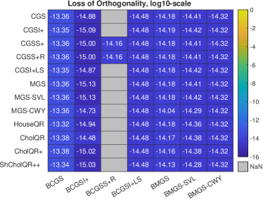
Figure 1: Measurements for rand_uniform

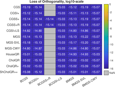
Figure 2: Measurements for rand_normal

3.2 rank_def

In Figure 3, we see that only the skeletons with reorthogonalization are robust enough to handle the matrix. It is further interesting to note that BCGSI+ performs nearly the same regardless of IntraOrtho.

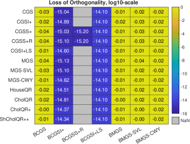
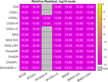
Figure 3: Measurements for rank_def

3.3 laeuchli

The Läuchli matrix reveals many interesting nuances. We first note in Figure 4 that for all algorithms that run to completion, except BCGSI+ with CGS, MGS, MGS-SVL, and MGS-CWY, the relative residual exceeds double precision. This is due to the nature of the Läuchli matrix itself: because entries are either zero or close to $\varepsilon$, there is a high rate of cancellation. Incidentally, this same cancellation is the reason that neither CholQR nor CholQR+ are viable IntraOrthos, and BCGSI+LS and BMGS-CWY are not viable skeletons: $\bm{X}_{1}^{T}\bm{X}_{1}$ is within $\mathcal{O}\left(\varepsilon\right)$ of a matrix of all ones, which is not strictly positive definite and therefore violates the requirements in Matlab’s chol.

The other interesting point relates to the correction matrix $T$ of MGS-SVL. Both BCGSI+ and BMGS suffer a total loss of orthogonality with MGS-SVL, but BMGS-SVL does not, since the BMGS-SVL skeleton was designed to incorporate this $T$ matrix from the MGS-SVL muscle. There is an easy fix for BCGSI+ and BMGS: we can incorporate the $T$ output of MGS-SVL into both algorithms by replacing every action of $\bm{Q}_{k}$ with $\bm{Q}_{k}T_{kk}$. The second loss of orthogonality table in Figure 4 demonstrates the outcome, with a “T” suffix denoting the altered algorithms. With the T-fix, both $\texttt{BCGSI+T}\circ\texttt{MGS-SVL}$ and $\texttt{BMGS-T}\circ\texttt{MGS-SVL}$ perform as well as $\texttt{BMGS-SVL}\circ\texttt{MGS-SVL}$; in fact, $\texttt{BCGSI+T}\circ\texttt{MGS-SVL}$ matches the others in residual too. (Note that BCGS with the T-fix would reproduce BMGS-SVL.) We note also that, even though MGS-SVL and MGS-CWY are based on the same projector, BMGS-SVL does not work with the muscle MGS-CWY; orthogonality is completely lost.

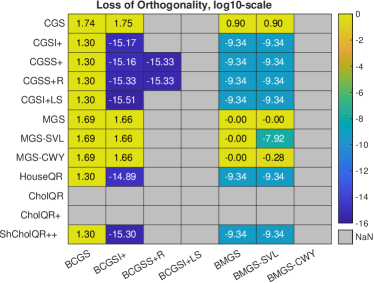
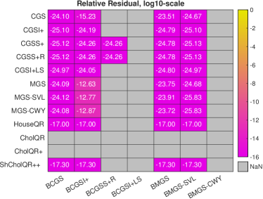
Figure 4: Measurements for laeuchli

3.4 monomial

The monomial matrix also reveals a few interesting properties. In Figure 5 we now see that all Cholesky-based methods can run, but they all lose quite a bit of orthogonality. Also, CGS in particular struggles across the board. We again see that $\texttt{BCGSI+}\circ\texttt{MGS-SVL}$ (and also $\texttt{BCGSI+}\circ\texttt{MGS-CWY}$) does not perform as well as other variants of BCGSI+; however, the T-fix will not provide any benefit here, because $\texttt{BCGSI+}\circ\texttt{MGS-SVL}$ is already as stable as $\texttt{BMGS-SVL}\circ\texttt{MGS-SVL}$.

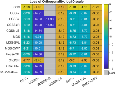
Figure 5: Measurements for monomial

3.5 s-step and newton

The s-step and newton matrices simulate behavior one would encounter when implementing s-step Krylov subspace methods; see, e.g., [5, 50, 24]. The s-step matrix is poorly conditioned, as expected, because a monomial is used to build the basis; for these particular parameters and test matrix it is even numerically singular. The newton matrix simulates what would happen when Newton polynomials are used instead, which leads to much better conditioning. It is interesting that only BCGSS+rpl is capable of factoring the s-step matrix; not even $\texttt{BCGSI+}\circ\texttt{HouseQR}$ is capable. One the other hand, both one-sync methods (BCGSI+LS and BMGS-CWY) factor newton satisfactorily, almost to full precision.

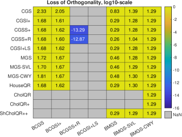
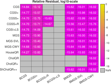
Figure 6: Measurements for s-step

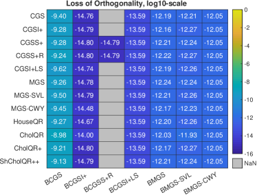
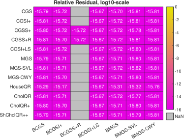
Figure 7: Measurements for newton

3.6 stewart

Stewart [36] purposefully designed his algorithms to be robust for pathologically bad matrices, and the results in Figure 8 demonstrate the failure of most algorithms for such matrices. Because of the identically zero column, nearly all methods encounter a NaN at some point after division of $0$ by $0$, which then spoils the rest of the algorithm. The only methods robust enough for such situations is Stewart’s own algorithm, $\texttt{BCGSS+rpl}\circ\texttt{CGSS+rpl}$, its variant without replacement, and BCGSI+ with Stewart’s IntraOrthos and HouseQR.

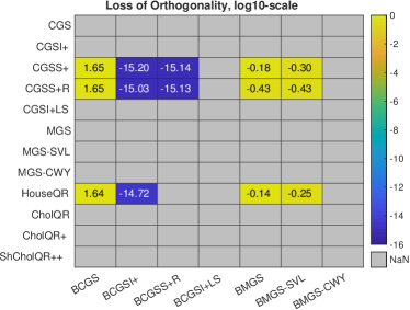
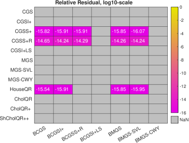
Figure 8: Measurements for stewart

3.7 stewart_extreme

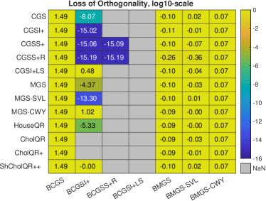
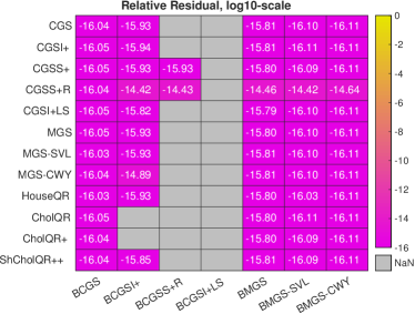
Figure 9: Measurements for stewart_extreme

This matrix in our collection demonstrates the utility of aggressive replacement. Figure 9 collects the results for stewart_extreme.

For both BCGSI+ and BCGSS+rpl we can see how aggressive replacement can make a significant difference. The only algorithms capable of achieving $\mathcal{O}\left(\varepsilon\right)$ loss of orthogonality in this case are BCGSS+rpl with CGSS+ and CGSS+rpl, and BCGSI+ with CGSS+, CGSS+rpl, and CGSI+. It is unclear why for this particular case $\texttt{BCGSI+}\circ\texttt{CGSI+}$ exhibits better orthogonality than $\texttt{BCGSI+}\circ\texttt{HouseQR}$.

Looking closely at Algorithm 4, we see that BCGSI+ does not reorthogonalize the first block vector in line 2, likely because this is not done for the column-wise algorithm, where it is unnecessary. By simply rerunning IntraOrtho for the first block vector (denoted “BCGSI+1” in Figure 9), we can reduce the loss of orthogonality to $\mathcal{O}\left(\varepsilon\right)$ for some muscles. Notably both the one-sync methods– CGSI+LS and MGS-CWY– still struggle, and CholQR still cannot run to completion.

This example highlights a problem that remains unaddressed in [13] for ShCholQR++: when $\bm{X}$ contains a column very close to the zero vector. In this situation, the bounds for the shift $\sigma$ may be too stringent to allow $\bm{X}^{T}\bm{X}+\sigma I_{s}$ to be numerically positive definite. In the stewart_extreme example, setting $\sigma=\left\lVert\bm{X}\right\rVert_{2}^{2}$ allows $\texttt{BCGSI+}\circ\texttt{ShCholQR++}$ to run to completion with $\mathcal{O}\left(10^{-12}\right)$ loss of orthogonality and $\mathcal{O}\left(10^{-17}\right)$ residual. It seems that the upper bound $\sigma\leq\frac{1}{100}\left\lVert\bm{X}\right\rVert_{2}^{2}$ is more likely an artifact of the analysis and that a larger bound may in fact be tolerable. To be fully robust, ShCholQR++ should be written to allow for an automatically tuned bound based on whether the shifted Gramian is found to be positive definite enough for chol to run. This remains a topic of future work.

We note that this trick of reorthogonalizing the first block vector has even better results for other test problems we tried. For both monomial and laeuchli, if we reorthogonalize the first block vector then BCGSI+ with any of the tested muscles provides $\mathcal{O}\left(\varepsilon\right)$ loss of orthogonality. We do not display these tests here, but see a related discussion in Section 4.2.

Overall, the experiments in this section give indication that different skeletons have very different requirements on the muscle. For BCGS, the choice of muscle makes little difference. This is because BCGS is itself unstable as a skeleton, so there is no benefit to using, say, HouseQR instead of CGS (as long as the constraints on condition number are satisfied to make the muscle viable). In constrast, the reorthogonalization in BCGSI+ stablizes the skeleton, and thus the quality of the IntraOrtho will have a greater affect on the resulting stability. This is also true for BMGS and variants like BMGS-SVL. We elaborate on these details in the following section.

4 Skeleton stability in terms of muscle stability: details

We now consider the stability of each skeleton in more detail. We utilize a common plot format, wherein stability quantities like loss of orthogonality or relative residual are plotted against varying condition numbers. We refer to such plots as $\kappa$-plots, where $\kappa$ refers to the fact that we study stability with respect to changes in condition number. The simplest version of these plots takes a series of matrices $\bm{\mathcal{X}}_{t}=\bm{\mathcal{U}}\Sigma_{t}\mathcal{V}^{T}\in\mathbb{R}^{m\times ps}$, where $\bm{\mathcal{U}}\in\mathbb{R}^{m\times ps}$ is orthonormal, $\Sigma_{t}\in\mathbb{R}^{ps\times ps}$ is a diagonal matrix whose entries are drawn from the logarithmic interval $10^{[-t,0]}$, and $\mathcal{V}\in\mathbb{R}^{ps\times ps}$ is unitary. We also consider glued $\kappa$-plots, where the matrices are instead built as the “glued” matrices from [28]; see C for how they are generated. The monomial matrices from Section 3 also lend themselves to $\kappa$-plots, because varying condition numbers can be induced by varying block sizes. All $\kappa$-plots are run in Matlab 9.8.0.1451342 (R2020a) Update 5. We provide the command-line calls for each figure in C.

4.1 BCGS

Using similar techniques as for CGS, we conjecture that the loss of orthogonality in $\texttt{BCGS}\circ\texttt{IntraOrtho}$ can be bounded as

$$\left\lVert I-\bar{\bm{\mathcal{Q}}}^{T}\bar{\bm{\mathcal{Q}}}\right\rVert_{2}\leq\mathcal{O}\left(\varepsilon\right)\kappa(\bm{\mathcal{X}})^{n-1}$$

as long as $\mathcal{O}\left(\varepsilon\right)\kappa(\bm{\mathcal{X}})<1$. A full proof that the BCGS $P$-variants have $\mathcal{O}\left(\varepsilon\right)\kappa^{2}(\bm{\mathcal{X}})$ loss of orthogonality and $\mathcal{O}\left(\varepsilon\right)$ relative Cholesky residual as long as $\mathcal{O}\left(\varepsilon\right)\kappa(\bm{\mathcal{X}})<1/2$ is given in [29]. These bounds hold as long as $\texttt{IntraOrtho}(\bm{X})$ satisfies

$$\bar{R}^{T}\bar{R}=\bm{X}^{T}\bm{X}+E,\quad\left\lVert E\right\rVert\leq\mathcal{O}\left(\varepsilon\right)\left\lVert\bm{X}\right\rVert^{2},$$ (10)

and

$$\bar{\bm{Q}}\bar{R}=\bm{X}+\bm{D},\quad\left\lVert\bm{D}\right\rVert\leq\mathcal{O}\left(\varepsilon\right)(\left\lVert\bm{X}\right\rVert+\left\lVert\bar{\bm{Q}}\right\rVert\left\lVert\bar{R}\right\rVert).$$ (11)

We note that these constraints on the IntraOrtho are relatively relaxed, and are satisfied by almost any reasonable choice of IntraOrtho, from CholQR to HouseQR. Indeed, in Figure 10, we see that both BCGS-PIP and BCGS-PIO (as well as BCGS) behave similarly for both CholQR and HouseQR. We also note that it is clear that BCGS (without the Pythagorean fix) does not satisfy the $\mathcal{O}\left(\varepsilon\right)\kappa^{2}{\bm{\mathcal{X}}}$ bound on loss of orthogonality; as the relative Cholesky residual departs from $\mathcal{O}\left(\varepsilon\right)$, the loss of orthogonality follows suit.

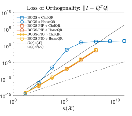
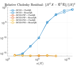
Figure 10: glued $\kappa$-plots for P-variants of BCGS.

4.2 BCGSI+

Barlow and Smoktunowicz prove an $\mathcal{O}\left(\varepsilon\right)$ loss of orthogonality for BCGSI+ and an unconditionally stable IntraOrtho, as long as $\mathcal{O}\left(\varepsilon\right)\kappa(\bm{\mathcal{X}})<1$ [16]. The key to their approach is to first obtain bounds for the following subproblem: given a near left-orthogonal matrix $\bm{\mathcal{U}}\in\mathbb{R}^{m\times t}$ and a matrix $\bm{B}\in\mathbb{R}^{m\times s}$, find an $\bm{S}\in\mathbb{R}^{t\times s}$, $R\in\mathbb{R}^{s\times s}$ upper triangular, and $\bm{Q}$ left orthogonal such that

$$\bm{B}=\bm{\mathcal{U}}\bm{S}_{\bm{B}}+\bm{Q}_{\bm{B}}R_{\bm{B}}\mbox{ and }\bm{\mathcal{U}}^{T}\bm{Q}_{\bm{B}}\approx 0.$$ (12)

This subproblem is present at every step of BCGSI+, as long as the previous step has produced a near-left orthogonal matrix $\bm{\mathcal{U}}$. With the unconditionally stable IntraOrtho guaranteeing that $\bm{Q}_{1}$ (see line 2 in Algorithm 4) is near left-orthogonal, induction over bounds on the subproblem leads to the desired result.

One potential drawback to Barlow and Smoktunowicz’s approach is the a posteriori assumption that $\mathcal{O}\left(\varepsilon\right)\left\lVert\bm{B}\right\rVert\left\lVert\bar{R}_{\bm{B}}^{-1}\right\rVert<1$, where $\bar{R}_{\bm{B}}$ is the computed version of $R_{\bm{B}}$ from the subproblem (12); see [16, Equation (3.27)]. In addition to simplifying the proof, the authors argue that such an assumption is useful in practice, because the computed quantities can be measured on the fly.

Figure 11 displays standard $\kappa$-plots for BCGSI+ in comparison to BCGS for muscles CGS, MGS, and HouseQR. It is tempting to conclude that the skeletons’ loss of orthogonality is independent of the muscle, but recalling the results for laeuchli and monomial matrices in Sections 3.3 and 3.4 (both of which satisfy $\mathcal{O}\left(\varepsilon\right)\kappa(\bm{\mathcal{X}})<1$; cf. Table 4), it is clear that we may need an unconditionally stable IntraOrtho for some tough matrices. Figure 12 shows $\kappa$-plots generated using laeuchli matrices. Indeed, here we see highlighted the different ways that BCGS and BCGSI+ are affected by the IntraOrtho. Whereas BCGS behaves the same regardless of what IntraOrtho is used, BCGSI+ is much more sensitive.

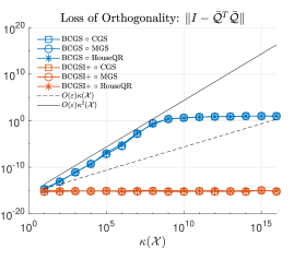
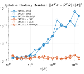
Figure 11: standard $\kappa$-plots for BCGSI+, in comparison to BCGS.

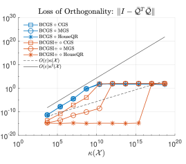
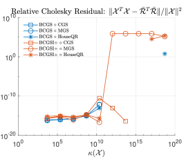
Figure 12: Laeuchli $\kappa$-plots for BCGSI+, in comparison to BCGS.

4.3 BCGSS+rpl

Although Stewart’s development of BCGSS+rpl [36] is largely driven by stability considerations, a rigorous proof is lacking. We conjecture that for any $\bm{\mathcal{X}}$, even those with rank deficiency, we have $\mathcal{O}\left(\varepsilon\right)$ loss of orthogonality, up to a small constant accounting for the replacement tolerance $\delta$.

This conjecture is based largely on numerical results from both Stewart’s paper [36] and our own studies in Section 3, wherein a clear trade-off between loss of orthogonality and relative residual seems to be driven largely by $\delta$. It is also clear that the orthogonalization fault step, designed precisely to avoid situations leading to instability, plays an important role. A successful stability analysis for BCGSS+rpl of course also depends on one for CGSS+rpl.

4.4 BCGSI+LS

Rigorous stability analysis for the low-sync algorithms from [25], especially their block versions, remains open. We can, however, formulate some conjectures.

In Figure 13, we see that indicate that BCGSI+LS remains relatively stable, especially its relative Cholesky residual. The loss of orthogonality for BCGSI+LS begins to deviate gradually from $\mathcal{O}\left(\varepsilon\right)$ in Figure 13. However, looking at the more challenging laeuchli matrix problems in Figure 14, we see that the loss of orthogonality can be much more significant, exceeding $\mathcal{O}\left(\varepsilon\right)\kappa(\bm{\mathcal{X}})$. Based on these results, we conjecture that BCGSI+LS satisfies the bound $\mathcal{O}\left(\varepsilon\right)\kappa^{2}(\bm{\mathcal{X}})$ as long as $\mathcal{O}\left(\varepsilon\right)\kappa^{2}(\bm{\mathcal{X}})<1$ (due to the use of chol within the algorithm). This conjecture is stated in Table 3; a formal proof remains future work. The norm lagging and delayed reorthogonalization seems to have a much more significant effect in BCGSI+LS versus CGSI+LS.

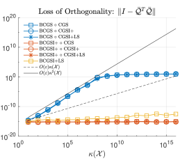
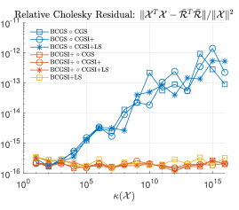
Figure 13: standard $\kappa$-plots for low-sync BCGSI+LS, in comparison to those of BCGS and BCGSI+.

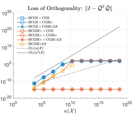
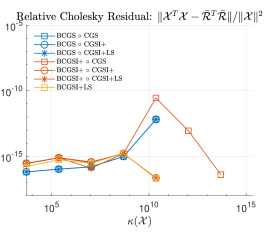
Figure 14: laeuchli $\kappa$-plots for low-sync BCGSI+LS, in comparison to those of BCGS and BCGSI+.

4.5 BMGS

What appears to be the earliest study on the stability of a block Gram-Schmidt method was conducted by Jalby and Philippe in 1991 [18]. They focus on $\texttt{BMGS}\circ\texttt{MGS}$ and $\texttt{BMGS}\circ\texttt{MGS+}$, and note how the underlying CGS-like nature of BMGS makes it prone to instability. To see this, observe that lines 4-8 of Algorithm 8 can be written more succinctly (in exact arithmetic) as

$$\bm{W}=(I-\bm{Q}_{k}\bm{Q}_{k}^{T})\cdots(I-\bm{Q}_{1}\bm{Q}_{1}^{T})\bm{X}_{k+1}.$$ (13)

Because each $\bm{Q}_{j}$, $j=1,\ldots,k$, here is a tall-and-skinny matrix, the projector $I-\bm{Q}_{j}\bm{Q}_{j}^{T}$ is equivalent to a step of CGS. The authors demonstrate this intuition rigorously with MGS as the IntraOrtho to arrive at the following bound for the loss of orthogonality:

$$\left\lVert I-\bar{\bm{\mathcal{Q}}}^{T}\bar{\bm{\mathcal{Q}}}\right\rVert_{2}\leq\mathcal{O}\left(\varepsilon\right)C\left\lVert\bm{\mathcal{X}}\right\rVert_{\text{F}}\left\lVert\mathcal{R}^{-1}\right\rVert_{2}\leq\mathcal{O}\left(\varepsilon\right)\kappa^{2}(\bm{\mathcal{X}}),$$ (14)

wherein the second inequality follows because $C\leq O(\kappa(\bm{\mathcal{X}}))$ and we have $\left\lVert\bm{\mathcal{X}}\right\rVert_{\text{F}}\left\lVert\mathcal{R}^{-1}\right\rVert_{2}\leq O(\kappa(\bm{\mathcal{X}}))$. The authors further show that the constant $C$ becomes $O(1)$ if MGS is replaced by MGS+, thus giving the MGS-like bound

$$\left\lVert I-\bar{\bm{\mathcal{Q}}}^{T}\bar{\bm{\mathcal{Q}}}\right\rVert_{2}\leq\mathcal{O}\left(\varepsilon\right)\kappa(\bm{\mathcal{X}}).$$ (15)

Barlow [15] conjectures that $\texttt{BMGS}\circ\texttt{HouseQR}$ is as stable as MGS but does not prove so explicitly. A careful look at Jalby and Philippe’s proof for their Theorem 4.1 reveals that there is not much to prove; in fact, the very same observation they used to derive (15) holds for any IntraOrtho that is unconditionally stable.

We sketch the proof of this here. At the top of page 1062 of [18], the Jalby and Philippe directly apply MGS bounds from [8] and define the constant $C=\max_{1\leq k\leq p-1}\left\lVert\bm{W}_{k}\right\rVert_{\text{F}}\left\lVert R_{\bm{W}_{k}}^{-1}\right\rVert_{2}$, where $\bm{W}_{k}$ corresponds to the block vector computed up to line 8 of Algorithm 8, and $R_{\bm{W}_{k}}$ its upper triangular factor from an exact QR decomposition. The intermediate constants $\left\lVert\bm{W}_{k}\right\rVert_{\text{F}}\left\lVert R_{\bm{W}_{k}}^{-1}\right\rVert_{2}$ are absent for any unconditionally stable IntraOrtho. Tracking $C$ all the way through the proof of [18, Theorem 4.1] (by which (14) holds) verifies that, without changing any other lines in their text, we would obtain (15) for $\texttt{BMGS}\circ\texttt{IntraOrtho}$, assuming IntraOrtho is unconditionally stable.

We remark that, to our knowledge, the present work is the first to state bounds for BMGS with an unconditionally stable IntraOrtho (such as HouseQR or TSQR), despite the ubiquity of $\texttt{BMGS}\circ\texttt{HouseQR}$ in practice. More precise bounds for particular IntraOrthos remain open, but can be easily derived on a case-by-case basis from the transparent analysis in [18].

Because $\texttt{BMGS}\circ\texttt{HouseQR}$ behaves essentially like MGS, we conjecture that results analogous to those by Paige, Rozložník, and Strakoš [11] hold for block GMRES, which is usually implemented with $\texttt{BMGS}\circ\texttt{HouseQR}$. To be more specific, the loss of orthogonality in $\texttt{BMGS}\circ\texttt{HouseQR}$ is tolerable when the end application is the solution of a linear system via the GMRES method.

Figure 15 demonstrates the BMGS behavior for a variety of muscles and their reorthogonalized variants again for both standard $\kappa$-plots (left) and laeuchli $\kappa$-plots (right). For the standard $\kappa$-plots, all variants behave the same, giving better orthogonality than indicated by (14). For the laeuchli $\kappa$-plots, we do observe behavior like (14) here for the IntraOrthos that do not have $\mathcal{O}\left(\varepsilon\right)$ loss of orthogonality (CGS, MGS, and CholQR). Indeed, this example demonstrates that an unconditionally stable muscle is really necessary to guarantee $\mathcal{O}\left(\varepsilon\right)\kappa(\bm{\mathcal{X}})$ loss of orthogonality.

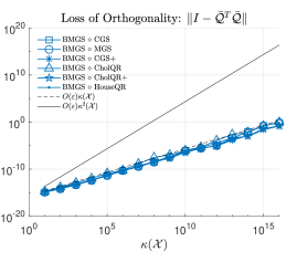
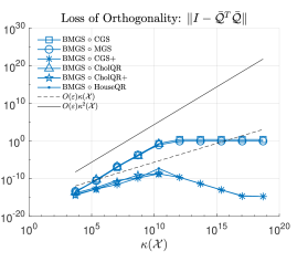
Figure 15: $\kappa$-plots for BMGS. (a) standard $\kappa$-plot. (b) laeuchli $\kappa$-plot.

(a)	(b)

4.6 Low-sync BMGS variants

To date, we are only aware of Barlow’s stability analysis of MGS-SVL and BMGS-SVL for low-synchronization BMGS variants [15]. Indeed, it appears that Barlow was even unaware that his algorithms could take on so many other forms, particularly the work by Świrydowicz et al. [25].

Barlow’s analysis relies heavily on the Sheffield observation and Schreiber-van-Loan reformulation– what is sometimes also referred to as the “augmented” problem– for the stability analysis of BMGS-SVL; see, in particular, [15, Section 4]. The following quantities play key roles:

$$\Delta_{\mathcal{T}\SS} :=\bar{\mathcal{T}}\SS-I,$$

$$\Delta_{\bar{\bm{\mathcal{Q}}}\bar{\mathcal{R}}} :=\bar{\bm{\mathcal{Q}}}\bar{\mathcal{R}}-\bm{\mathcal{X}},\mbox{ and }$$

$$\Gamma_{\mathcal{T}\mathcal{R}} :=(I-\bar{\mathcal{T}})\bar{\mathcal{R}}.$$

The matrix $\SS\in\mathbb{R}^{n\times n}$ is an exact quantity that does not explicitly arise in the computation. Although it has several equivalent formulations in exact arithmetic (see especially page 1261 in [15]), it is apparently defined as the upper triangular part of the exact multiplication between $\bar{\bm{\mathcal{Q}}}^{T}$ and $\bar{\bm{\mathcal{Q}}}$, i.e.,

$$\SS:=\texttt{triu}(\bar{\bm{\mathcal{Q}}}^{T}\bar{\bm{\mathcal{Q}}}).$$

In exact arithmetic, $\SS=\mathcal{T}^{-1}$, hence why the measure $\Delta_{\mathcal{T}\SS}$ bears significance.

For $\texttt{BMGS-SVL}\circ\texttt{IntraOrtho}$, Barlow shows that

$$\left\lVert\Delta_{\mathcal{T}\SS}\right\rVert_{\text{F}} \leq\mathcal{O}\left(\varepsilon\right),$$ (16)

$$\left\lVert\Delta_{\bar{\bm{\mathcal{Q}}}\bar{\mathcal{R}}}\right\rVert_{\text{F}} \leq\mathcal{O}\left(\varepsilon\right)\left\lVert\bm{\mathcal{X}}\right\rVert_{\text{F}},\mbox{ and }$$ (17)

$$\left\lVert\Gamma_{\mathcal{T}\mathcal{R}}\right\rVert_{\text{F}} \leq\mathcal{O}\left(\varepsilon\right)\left\lVert\bm{\mathcal{X}}\right\rVert_{\text{F}},$$ (18)

as long as $[\bar{\bm{Q}},\bar{R},\bar{T}]=\texttt{IntraOrtho}\left(\bm{X}\right)$ satisfies the triad

$$\Delta_{TS} :=\bar{T}S-I_{s},\quad\left\lVert\Delta_{TS}\right\rVert_{\text{F}}\leq\mathcal{O}\left(\varepsilon\right);$$ (19)

$$\Delta_{\bar{\bm{Q}}\bar{R}} :=\bar{\bm{Q}}\bar{R}-\bm{X},\quad\left\lVert\Delta_{\bar{\bm{Q}}\bar{R}}\right\rVert_{\text{F}}\leq\mathcal{O}\left(\varepsilon\right)\left\lVert\bm{X}\right\rVert_{\text{F}};\mbox{ and }$$ (20)

$$\Gamma_{TR} :=(I_{s}-\bar{T})\bar{R},\quad\left\lVert\Gamma_{TR}\right\rVert_{\text{F}}\leq\mathcal{O}\left(\varepsilon\right)\left\lVert\bm{X}\right\rVert_{\text{F}}$$ (21)

where $S:=\texttt{triu}(\bar{\bm{Q}}^{T}\bar{\bm{Q}})$ and $S=T^{-1}$ in exact arithmetic.

Equation (17) already gives the usual residual bound, and Barlow additionally shows that it holds at every step of BMGS. To arrive at bounds for loss of orthogonality, he further shows that (16)-(18) imply

$$\left\lVert I-\bar{\bm{\mathcal{Q}}}^{T}\bar{\bm{\mathcal{Q}}}\right\rVert_{\text{F}}\leq\mathcal{O}\left(\varepsilon\right)\left\lVert\bm{\mathcal{X}}\right\rVert_{\text{F}}\left\lVert\mathcal{R}^{-1}\right\rVert,$$

Recalling (from, e.g., [8]) that $\left\lVert\bm{\mathcal{X}}\right\rVert_{\text{F}}\left\lVert\mathcal{R}^{-1}\right\rVert\leq O(\kappa(\bm{\mathcal{X}}))$, this latter condition can be satisfied only if $\bm{\mathcal{X}}$ is sufficiently far from a rank-deficient matrix, i.e., if $\mathcal{O}\left(\varepsilon\right)\kappa(\bm{\mathcal{X}})<1$. We then have that

$$\left\lVert I-\bar{\bm{\mathcal{Q}}}^{T}\bar{\bm{\mathcal{Q}}}\right\rVert_{\text{F}}\leq\mathcal{O}\left(\varepsilon\right)\kappa(\bm{\mathcal{X}}),$$

and thanks to norm equivalence, we obtain the bounds reported in Table 3.

At first glance through A, it may seem that the MGS low-sync variants are the only muscles designed to produce a $T$ matrix. Upon further investigation of how Barlow uses the quantities $\Delta_{TS}$, $\Delta_{\bar{\bm{Q}}\bar{R}}$, and $\Gamma_{TR}$, it becomes clear that actually all other IntraOrthos implicitly produce $\bar{T}\equiv I$. This is important for composing BMGS-SVL and BMGS-LTS with other muscles, because they explicitly update the block diagonal entries of $\mathcal{T}$ with outputs from the IntraOrtho.

It then holds for these muscles that

$$\left\lVert\Delta_{TS}\right\rVert_{\text{F}}\equiv\left\lVert\texttt{triu}(I-\bar{\bm{Q}}^{T}\bar{\bm{Q}})\right\rVert_{\text{F}}\leq\left\lVert I-\bar{\bm{Q}}^{T}\bar{\bm{Q}}\right\rVert_{\text{F}},$$

and

$$\left\lVert\Gamma_{TR}\right\rVert_{\text{F}}=0.$$

Is is thus clear that (19)-(21) are satisfied by any IntraOrtho with $\mathcal{O}\left(\varepsilon\right)$ loss of orthogonality and relative residual (such as CGSI+), and thus (16)-(18) hold. Note that although MGS-SVL does not have $\mathcal{O}\left(\varepsilon\right)$ loss of orthogonality, it still satisfies (19)-(21) as long as $\bar{R}$ is assumed to be nonsingular; this is proved directly by Barlow (see [15, Section 4.2]). We conjecture that Barlow’s framework could be easily repurposed to prove rigorous stability bounds for MGS-LTS and BMGS-LTS. A full stability analysis for MGS-LTS, MGS-CWY, and MGS-ICWY and their block variants is the subject of ongoing work.

In Figure 16, we focus on just the BMGS-SVL skeleton and its one-sync version, BMGS-CWY, paired with all four “T”-variants as muscles as well as HouseQR. Standard $\kappa$-plots are on the left and laeuchli $\kappa$-plots are on the right. For the standard $\kappa$-plots, the behavior of all variants is nearly identical, achieving $\mathcal{O}\left(\varepsilon\right)$ loss of orthogonality. The more challenging laeuchli matrices are more discerning, allowing us to draw two main conclusions. First, the T-variant skeletons and muscles are not “mix-and-match”; BMGS-SVL works with MGS-SVL, but in combination with other T-variant muscles, the loss of orthogonality exceeds the $\mathcal{O}\left(\varepsilon\right)\kappa(\bm{\mathcal{X}})$ bound. Second, as with BCGSI+LS (cf. Section 4.4), normalization lagging in BMGS-CWY can lead to complete loss of orthogonality. Here, BMGS-CWY loses orthogonality completely after $\mathcal{O}\left(\varepsilon\right)\kappa^{2}(\bm{\mathcal{X}})$ exceeds 1, even when combined with an unconditionally stable muscle like HouseQR.

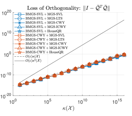
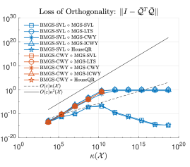
Figure 16: $\kappa$-plots for low-sync variants of BMGS. (a) standard $\kappa$-plot. (b) laeuchli $\kappa$-plot.

(a)	(b)

5 Mixed-precision approaches

Due to the trend of commercially available mixed-precision hardware and its potential to provide computational time and energy savings, there is a growing interest in the use of mixed precision within numerical linear algebra routines. We comment briefly on existing efforts towards mixed-precision orthogonalization schemes.

In [51], a mixed-precision Cholesky QR factorization (mCholQR) is studied, in which some intermediate computations are performed at double the working precision. The authors prove that in such a mixed-precision setting, the loss of orthogonality depends only linearly (rather than quadratically) on the condition number of the input matrix under the assumption (as in CholQR) that $\mathcal{O}\left(\varepsilon\right)\kappa^{2}(\bm{X})<1$ (cf. Table 2).

Building on this work, in [52], the authors propose using the mCholQR of [51] as the IntraOrtho within BGS. The paper does not contain a formal error analysis, but various numerical experiments are performed to examine the loss of orthogonality and residual error when mCholQR is combined with BMGS and BCGS. The experiments suggest that in some cases the numerical stability of the $\texttt{BMGS}\circ\texttt{mCholQR}$ variants can be maintained to the same level of MGS if reorthogonalization is used.

We note also that in [53], the finite-precision behavior of HouseQR and its blocked variants is analyzed in various mixed-precision settings. The potential performance benefits of mixed precision make the study of the stability properties of mixed-precision BGS variants of great interest going forward.

6 Software Frameworks

In the following, we highlight which variants of BGS are implemented in well-known software packages.

To our knowledge, the Trilinos Library, in particular the Belos package, provides the most opportunity for the user to select among various orthogonalization schemes to be used within Krylov subspace methods. Belos currently contains implementations of TSQR, iterated CGS and MGS, and CGSS+. For block Krylov subspace methods, Belos implements various BGS methods. For example, in block GMRES, the user may choose between block versions of iterated CGS and MGS, and CGSS+, the default being block iterated CGS. A recent presentation [54] on the Trilinos Library presents experiments with communication-avoiding ($s$-step) GMRES using $\texttt{CGS}\circ\texttt{CholQR}$ as well as a “low-sync CGS” with CholQR+ as the IntraOrtho. We also note that $s$-step GMRES with low-sync block Gram-Schmidt orthogonalization algorithms including BCGS-PIP, BMGS-ICWY, and BCGSI+LS is described in the recent paper by Yamazaki et al. [30]. The authors demonstrate significant parallel scaling improvements over the previous Trilinos implementations of these KSM algorithms and lower time-to-solution for the iterative solver. The implementation of communication-avoiding Krylov subspace methods and associated block orthogonalization schemes, in particular low-synch variants, is a goal of the ongoing Exascale Computing Project PEEKS effort.

Block variants of GMRES, CG, break-down free CG and recycling GCRO Krylov solvers have all been implemented recently in PETSc as described in the paper by Jolivet et al. [55]. The authors also describe blocked eigensolvers employed within the PETSc software framework that are based on SLEPc. These employ the Locally Optimal Block Preconditioned Conjugate Gradient (LOBPCG) algorithm due to Knyazev [56] and the Contour Integral Spectrum Slicing method (CISS) of Sakurai and Suguria [57].

For prototype algorithms and testing routines for stability conjectures, we direct the reader to the Matlab package developed in conjunction with this survey, hosted at https://github.com/katlund/BlockStab.

7 Conclusions and outlook

The take-home lesson of stability studies is always the same, but often forgotten: be careful, because the finite precision universe can behave in exceptionally undesirable ways, especially if you have only analyzed your method in exact arithmetic. At the same time, when an algorithm works well “most of the time,” there are probably good reasons, and we should be realistic about the statistical likelihood that something catastrophic may occur, especially if the algorithm is providing massive benefit in other ways.

Sometimes, however, stability may be a stringent requirement for a software pipeline. This is especially true if eigenvalue estimates are needed anywhere [2]. Lately, Krylov subspace methods, and particularly block Krylov subspace methods, form an important component in matrix function approximations, which often use eigenvalue estimations to accelerate convergence [58, 59, 60, 61, 62]. Other applications where reliable eigenvalue estimates are needed include Krylov subspace recycling and spectral deflation [63, 64].

It is also worth exploring whether the low-sync BGS variants – BCGSI+LS, BMGS-SVL, BMGS-LTS, BMGS-CWY, BMGS-ICWY– coupled with muscles such as TSQR or ShCholQR++, provide similar communication benefits as $\texttt{BCGS}\circ\texttt{TSQR}$ but with better stability properties. This is especially relevant for $s$-step KSMs, which rely on the low communication of BCGS but can also suffer from its instability.

Although our focus has been on the stability properties of block orthogonalization routines, an overarching goal is to be able to say something about the backward stability of block (and $s$-step) variants of GMRES methods. Paige, Rozložník, and Strakoš have proven that (non-block) GMRES with MGS orthogonalization is backward stable, despite loss of orthogonality of the Arnoldi basis vectors due to the finite precision MGS computation [11]. It remains an open problem, even in the non-blocked case, to determine the level to which orthogonality can be lost in the finite precision orthogonalization routine while still obtaining a backward stable GMRES solution. Further, theoretical treatment of the backward stability of block Arnoldi/GMRES methods is entirely lacking from the literature. We hope that the present work provides a path forward in this direction, and a detailed application of the BGS results compiled here to block GMRES and methods like $s$-step GMRES remains as future work. The natural next step is an examination of the least-squares problem for block upper Hessenberg matrices. Work by Gutknecht and Schmelzer [65] may prove relevant, as well as the low-rank update formulation devised in [61] for matrix functions.

Appendix A Pseudocode for muscles

Algorithm 13 $[\bm{Q},R]=\texttt{CGS}(\bm{X})$

1:  $\bm{Q}=\bm{X}$

2:  for $k=1,\ldots,n$ do

3:     $R_{1:k-1,k}=\bm{Q}_{:,1:k-1}^{T}\bm{X}_{:,k}$

4:     $\bm{Q}_{:,k}=X_{:,k}-\bm{Q}_{:,1:k-1}R_{1:k-1,k}$

5:     $R_{k,k}=\|\bm{Q}_{:,k}\|$

6:     $\bm{Q}_{:,k}=\bm{Q}_{:,k}/R_{k,k}$

7:  end for

8:  return  $\bm{Q}$, $R$

Algorithm 14 $[\bm{Q},R]=\texttt{MGS}(\bm{X})$

1:  $\bm{Q}=\bm{X}$

2:  for $k=1,\ldots,n$ do

3:     $R_{k,k}=\|\bm{Q}_{:,k}\|$

4:     $\bm{Q}_{:,k}=\bm{Q}_{:,k}/R_{k,k}$

5:     $R_{k,k+1:n}=Q_{:,k}^{T}Q_{:,k+1:n}$

6:     $Q_{:,k+1:n}=Q_{:,k+1:n}-Q_{:,k}R_{k,k+1:n}$

7:  end for

8:  return  $\bm{Q}$, $R$

Algorithm 15 $[\bm{Q},\bm{R}]=\texttt{CGSS+rpl}(\bm{X},\delta)$

1:  Allocate memory for $\bm{Q}$ and $R$

2:  $[\bm{q}_{1},\sim,r_{11}]=\texttt{cgs\_step\_sror}(\bm{0},\bm{x}_{1},\delta)$

3:  for $k=1,\ldots,s-1$ do

4:     $[\bm{q}_{k+1},R_{1:k,k+1},r_{k+1,k+1}]=\texttt{cgs\_step\_sror}(\bm{Q}_{1:k},\bm{x}_{k+1},\delta)$

5:  end for

6:  return  $\bm{Q}=[\bm{q}_{1},\ldots,\bm{q}_{s}]$, $R=(r_{jk})$

Algorithm 16 $[\bm{Q},R,T]=\texttt{MGS-SVL}(\bm{X})$

1:  Allocate memory for $\bm{Q}$ and $R$

2:  $T=I_{s}$

3:  $r_{11}=\left\lVert\bm{x}_{1}\right\rVert$; $\bm{q}_{1}=\bm{x}_{1}/r_{11}$

4:  for $k=1,\ldots,s-1$ do

5:     $\bm{w}=\bm{x}_{k+1}$

6:     $R_{1:k,k+1}={\color[rgb]{1,0,0}T_{1:k,1:k}^{T}}\big{(}\bm{Q}_{1:k}^{T}\bm{w}\big{)}$

7:     $\bm{w}=\bm{w}-\bm{Q}_{1:k}R_{1:k,k+1}$

8:     $r_{k+1,k+1}=\left\lVert\bm{w}\right\rVert$

9:     $\bm{q}_{k+1}=\bm{w}/r_{k+1,k+1}$

10:     $T_{1:k,k+1}=-T_{1:k,1:k}\big{(}\bm{Q}_{1:k}^{T}\bm{q}_{k+1}\big{)}$

11:  end for

12:  return  $\bm{Q}=[\bm{q}_{1},\ldots,\bm{q}_{s}]$, $R=(r_{jk})$, $T=(t_{jk})$

Algorithm 17 $[\bm{Q},R,T]=\texttt{MGS-LTS}(\bm{X})$

1:  Allocate memory for $\bm{Q}$ and $R$

2:  $T=I_{s}$

3:  $r_{11}=\left\lVert\bm{x}_{1}\right\rVert$; $\bm{q}_{1}=\bm{x}_{1}/r_{11}$

4:  for $k=1,\ldots,s-1$ do

5:     $\bm{w}=\bm{x}_{k+1}$

6:     $R_{1:k,k+1}={\color[rgb]{1,0,0}T_{1:k,1:k}^{-T}}\big{(}\bm{Q}_{1:k}^{T}\bm{w}\big{)}$

7:     $\bm{w}=\bm{w}-\bm{Q}_{1:k}R_{1:k,k+1}$

8:     $r_{k+1,k+1}=\left\lVert\bm{w}\right\rVert$

9:     $\bm{q}_{k+1}=\bm{w}/r_{k+1,k+1}$

10:     $T_{1:k,k+1}=\bm{Q}_{1:k}^{T}\bm{q}_{k+1}$

11:  end for

12:  return  $\bm{Q}=[\bm{q}_{1},\ldots,\bm{q}_{s}]$, $R=(r_{jk})$, $T=(t_{jk})$

Algorithm 18 $[\bm{Q},R,T]=\texttt{MGS-CWY}(\bm{X})$

1:  Allocate memory for $\bm{Q}$ and $R$

2:  $T=I_{s}$

3:  $\bm{u}=\bm{x}_{1}$

4:  for $k=1,\ldots,s-1$ do

5:     $\bm{w}=\bm{x}_{k+1}$

6:     if $k=1$ then

7:        $\begin{bmatrix}r_{k,k}^{2}&\rho\end{bmatrix}=\bm{u}^{T}[\bm{u}\,\,\bm{w}]$

8:     else if $k>1$ then

9:        $\begin{bmatrix}\bm{t}&\bm{r}\\ r_{k,k}^{2}&\rho\end{bmatrix}=[\bm{Q}_{1:k-1}\,\,\bm{u}]^{T}[\bm{u}\,\,\bm{w}]$

10:        $T_{1:k-1,k}={\color[rgb]{1,0,0}-T_{1:k-1,1:k-1}(\bm{t}/r_{k,k})}$

11:     end if

12:     $R_{1:k,k+1}={\color[rgb]{1,0,0}T_{1:k,1:k}^{T}}\begin{bmatrix}\bm{r}\\ \rho/r_{k,k}\end{bmatrix}$

13:     $\bm{q}_{k}=\bm{u}/r_{k,k}$

14:     $\bm{u}=\bm{w}-\bm{Q}_{:,1:k}R_{1:k,k+1}$

15:  end for

16:  $r_{s,s}=\left\lVert\bm{u}\right\rVert$

17:  $\bm{q}_{s}=\bm{u}/r_{s,s}$

18:  return  $\bm{Q}=[\bm{q}_{1},\ldots,\bm{q}_{s}]$, $R=(r_{jk})$, $T=(t_{jk})$

Algorithm 19 $[\bm{Q},R,T]=\texttt{MGS-ICWY}(\bm{X})$

1:  Allocate memory for $\bm{Q}$ and $R$

2:  $T=I_{s}$

3:  $\bm{u}=\bm{x}_{1}$

4:  for $k=1,\ldots,s-1$ do

5:     $\bm{w}=\bm{x}_{k+1}$

6:     if $k=1$ then

7:        $\begin{bmatrix}r_{k,k}^{2}&\rho\end{bmatrix}=\bm{u}^{T}[\bm{u}\,\,\bm{w}]$

8:     else if $k>1$ then

9:        $\begin{bmatrix}\bm{t}&\bm{r}\\ r_{k,k}^{2}&\rho\end{bmatrix}=[\bm{Q}_{1:k-1}\,\,\bm{u}]^{T}[\bm{u}\,\,\bm{w}]$

10:        $T_{1:k-1,k}={\color[rgb]{1,0,0}\bm{t}/r_{k,k}}$

11:     end if

12:     $R_{1:k,k+1}={\color[rgb]{1,0,0}T_{1:k,1:k}^{-T}}\begin{bmatrix}\bm{r}\\ \rho/r_{k,k}\end{bmatrix}$

13:     $\bm{q}_{s}=\bm{u}/r_{s,s}$

14:     $\bm{u}=\bm{w}-\bm{Q}_{:,1:k}R_{1:k,k+1}$

15:  end for

16:  $r_{s,s}=\left\lVert\bm{u}\right\rVert$

17:  $\bm{q}_{s}=\bm{u}/r_{s,s}$

18:  return  $\bm{Q}=[\bm{q}_{1},\ldots,\bm{q}_{s}]$, $R=(r_{jk})$, $T=(t_{jk})$

Algorithm 20 $[\bm{Q},R]=\texttt{CholQR}(\bm{X})$

1:  $X=\bm{X}^{T}\bm{X}$

2:  if $X$ is positive definite then

3:     $R=\texttt{chol}(X)$

4:     $\bm{Q}=\bm{X}R^{-1}$

5:  else

6:     return  $\bm{Q}=\texttt{NaN}$, $R=\texttt{NaN}$

7:  end if

8:  return  $\bm{Q}$, $R$

Algorithm 21 $[\bm{Q},R]=\texttt{CholQR+}(\bm{X})$

1:  $[\bm{Q},R^{(1)}]=\texttt{CholQR}(\bm{X})$

2:  $[\bm{Q},R^{(2)}]=\texttt{CholQR}(\bm{Q})$

3:  $R=R^{(2)}R^{(1)}$

4:  return  $\bm{Q}$, $R$

Algorithm 22 $[\bm{Q},R]=\texttt{ShCholQR++}(\bm{X})$

1:  Define shift $\sigma=11(ms+s(s+1))\varepsilon\left\lVert\bm{X}\right\rVert_{2}^{2}$

2:  $R^{(1)}=\texttt{chol}(\bm{X}^{T}\bm{X}+\sigma I_{s})$

3:  $\bm{Q}=\bm{X}(R^{(1)})^{-1}$

4:  $[\bm{Q},R^{(2)}]=\texttt{CholQR+}(\bm{Q})$

5:  $R=R^{(2)}R^{(1)}$

Appendix B Matlab code for routines in BCGSS+rpl and CGSS+rpl

ΨΨfunction [y, r, rho, northog] = cgs_step_sror(Q, x, nu, rpltol)
ΨΨ% [y, r, rho, northog] = CGS_STEP_SROR(Q, x, nu, rpltol) orthogonalizes x
ΨΨ% against the columns of Q using the the Classical Gram-Schmidt method.
ΨΨ% Reorthogonalization is performed as necessary to ensure orthogonality.
ΨΨ% Specifically, given an orthonormal matrix Q and a vector x, the function
ΨΨ% returns a vectors y and r, and a scalar rho satisfying
ΨΨ%
ΨΨ% (*)   x = Q*r + rho*y
ΨΨ%
ΨΨ% where y is a normalized vector orthogonal to the column space of Q.
ΨΨ% The matrix Q may have zero columns.
ΨΨ%
ΨΨ% The optional argument nu is the norm of the original value of x, to be
ΨΨ% used when x has been subject to previous orthogonalizaton steps.  If
ΨΨ% nu is absent or is less than or equal to norm(x), is is set to norm(x).
ΨΨ%
ΨΨ% The optional argument rlptol controls when the current vector y is
ΨΨ% replaced by a random vector.  Its default value is 1.  If it is set
ΨΨ% to a value greater than one, the relation (*) will be compromised
ΨΨ% somewhat, but the number of orthogonalizations may be decreased.
ΨΨ%
ΨΨ% The optional output argument northog, if present, contains the number
ΨΨ% of orthogonalizations.
ΨΨ%
ΨΨ% Originally written by G. W. Stewart, 2008. Modified by Kathryn Lund,
ΨΨ% 2020.
ΨΨ
ΨΨ%%
ΨΨ% Initialize
ΨΨ[n, nq] = size(Q);
ΨΨr = zeros(nq, 1);
ΨΨnux = norm(x);
ΨΨif nargout >= 4
ΨΨnorthog = 0;
ΨΨend
ΨΨ
ΨΨ% If Q has no columns, return normalized x if x~=0, otherwise return a
ΨΨ% normalized random vector.
ΨΨif nq == 0
ΨΨif nux == 0
ΨΨy = rand(n,1)-0.5;
ΨΨy = y/norm(y);
ΨΨrho = 0;
ΨΨelse
ΨΨy = x/nux;
ΨΨrho = nux;
ΨΨend
ΨΨreturn
ΨΨend
ΨΨ
ΨΨ%  If required, intitalize the optional arguments nu and rpltol.
ΨΨif nargin < 3
ΨΨnu = nux;
ΨΨelse
ΨΨif nu < nux
ΨΨnu = nux;
ΨΨend
ΨΨend
ΨΨ
ΨΨif nargin < 4
ΨΨrpltol = 1;
ΨΨend
ΨΨ
ΨΨ% If norm(x)==0, set it to a nonzero vector and proceed, noting the fact in
ΨΨ% the flag zeronorm.
ΨΨif nux ~= 0
ΨΨzeronorm = false;
ΨΨy = x/nux;
ΨΨnu = nu/nux;
ΨΨelse
ΨΨzeronorm = true;
ΨΨy = rand(n,1) - 0.5;
ΨΨy = y/norm(y);
ΨΨnu = 1;
ΨΨend
ΨΨ
ΨΨ% Main orthogonalization loop.
ΨΨnu1 = nu;
ΨΨwhile true
ΨΨif nargout == 4
ΨΨnorthog = northog + 1;
ΨΨend
ΨΨs = Q’*y;
ΨΨr = r + s;
ΨΨy = y - Q*s;
ΨΨnu2 = norm(y);
ΨΨ
ΨΨ% Return if y is orthogonal.
ΨΨif nu2 > 0.5*nu1
ΨΨbreak
ΨΨend
ΨΨ
ΨΨ% Continue orthogonalizing if nu2 is not too small.
ΨΨif nu2 > rpltol*nu*eps
ΨΨnu1 = nu2;
ΨΨelse % Replace y by a random vector.
ΨΨnu = nu*eps;
ΨΨnu1 = nu;
ΨΨy = rand(n,1) - 0.5;
ΨΨy = nu*y/norm(y);
ΨΨend
ΨΨend
ΨΨ
ΨΨ% Calculate rho and normalize y.
ΨΨif ~zeronorm
ΨΨrho = norm(y);
ΨΨy = y/rho;
ΨΨrho = rho*nux;
ΨΨr = r*nux;
ΨΨelse
ΨΨy = y/norm(y);
ΨΨr = zeros(nq, 1);
ΨΨrho = 0;
ΨΨend
Ψ

ΨΨfunction [Y, R12, R22] = bcgs_step_sror(QQ, X, rpltol)
ΨΨ% [Y, R12, R22] = BCGS_STEP_SROR(QQ, X, rpltol) returns an orthonormal
ΨΨ% matrix Y whose columns lie in the orthogonal complement of the column
ΨΨ% space of QQ, a matrix R12, and an upper triangular matrix R22 satisfying
ΨΨ%
ΨΨ% (*)   X = QQ*R12 + Y*R22.
ΨΨ%
ΨΨ% The optional argument rpltol has a default value of 1.  Increasing it,
ΨΨ% say to 100, may improve performance, but will degrade the accuracy of the
ΨΨ% relation (*).
ΨΨ%
ΨΨ% Originally written by G. W. Stewart, 2008.  Modified by Kathryn Lund,
ΨΨ% 2020.
ΨΨ
ΨΨ%%
ΨΨ%  Initialization.
ΨΨreorth = false;
ΨΨif nargin < 3
ΨΨΨrpltol = 1;
ΨΨelse
ΨΨΨΨif rpltol < 1
ΨΨΨΨΨΨrpltol = 1;
ΨΨΨΨend
ΨΨend

ΨΨs = size(X,2);
ΨΨsk = size(QQ,2);

ΨΨnu = zeros(1,s);
ΨΨfor k = 1:s
ΨΨΨnu(k) = norm(X(:,k));
ΨΨend

ΨΨ%  Beginning of the first orthogonalization step.  Project Y
ΨΨ%  onto the orthogonal complement of Q.
ΨΨR12 = QQ’*X;
ΨΨY = X - QQ*R12;
ΨΨR22 = zeros(s);

ΨΨ%  Orthogonalize the columns of Y.
ΨΨfor k = 1:s
ΨΨΨΨ[yk, r, rho] = cgs_step_sror(Y(:,1:k-1), Y(:,k), nu(k), rpltol);
ΨΨΨΨY(:,k) = yk;
ΨΨΨΨR22(1:k-1,k) = r;
ΨΨΨΨR22(k,k) = rho;
ΨΨΨΨif rho <= 0.5*nu(k)
ΨΨΨΨΨΨreorth = true;
ΨΨΨΨend
ΨΨend

ΨΨ%  Return if Q has zero columns.
ΨΨif sk == 0 || ~reorth
ΨΨΨ return
ΨΨend

ΨΨ% Beginning of the reorthogonalization.  Project Y onto the orthogonal
ΨΨ% complement of Q.
ΨΨS12 = QQ’*Y;
ΨΨY = Y - QQ*S12;

ΨΨ% Orthogonalize the columns of Y.
ΨΨS22 = zeros(s);
ΨΨfor k = 1:s
ΨΨΨΨ[yk, r, sig] = cgs_step_sror(Y(:,1:k-1), Y(:,k), 1, rpltol);

ΨΨΨΨif sig < 0.5
ΨΨΨΨ% The result, yk, is not satisfactorily orthogonal.  Perform an
ΨΨΨΨ% unblocked orthogonalization against Q and the previous columns of Y.
ΨΨΨΨΨΨ[yk, r, sig] = cgs_step_sror([QQ, Y(:,1:k-1)], Y(:,k), rpltol);
ΨΨΨΨΨΨS12(:,k) = S12(:,k) + r(1:sk);
ΨΨΨΨΨΨr = r(sk+1:sk+k-1);
ΨΨΨΨend
ΨΨΨΨY(:,k) = yk;
ΨΨΨΨS22(1:k-1,k) = r;
ΨΨΨΨS22(k,k) = sig;
ΨΨend

ΨΨR12 = R12 + S12*R22;
ΨΨR22 = S22*R22;
ΨΨend
Ψ

Appendix C Glued matrices and command-line calls

Glued matrices are generated by the following Matlab code, modified from [28]:

Ψfunction A = CreateGluedMatrix(m, p, s, r, t)
Ψ% Example 2 matrix from [Smoktunowicz et al., 2006]. Generates a glued
Ψ% matrix of size m x ps, with parameters r and t specifying the powers of
Ψ% the largest condition number of the first stage and second stages of the
Ψ% matrix, respectively:
Ψ%
Ψ% Stage 1: A = U * Sigma * V’
Ψ%
Ψ% Stage 2: A = A * kron(I, Sigma_block) * kron(I, V_block)
Ψ
Ψ%%
Ψn = p * s;
ΨU = orth(randn(m,n));
ΨV = orth(randn(n,m));
ΨSigma = diag(logspace(0, r, n));
ΨA = U * Sigma * V’;
Ψ
ΨSigma_block = diag(logspace(0, t, s));
ΨV_block = orth(randn(s,s));
Ψ
Ψind = 1:s;
Ψfor i = 1:p
ΨΨA(:,ind) = A(:,ind) * Sigma_block * V_block’;
ΨΨind = ind + s;
Ψend
Ψend
Ψ

All the heat-maps in Section 3 can be reproduced with the code hosted at https://github.com/katlund/BlockStab and the following commands:

XXdim = [10000 50 10];
mat = {’rand_uniform’, ’rand_normal’, ’rank_def’, ’laeuchli’,...
    ’monomial’, ’stewart’, ’stewart_extreme’, ’hilbert’,...
    ’s-step’, ’newton’};
skel = {’BCGS’, ’BCGS_IRO’, ’BCGS_SROR’, ’BCGS_IRO_LS’,...
    ’BMGS’, ’BMGS_SVL’, ’BMGS_CWY’};
musc = {’CGS’, ’CGS_IRO’, ’CGS_SRO’, ’CGS_SROR’,...
    ’CGS_IRO_LS’, ’MGS’, ’MGS_SVL’, ’MGS_CWY’, ’HouseQR’,...
    ’CholQR’, ’CholQR_RO’, ’Sh_CholQR_RORO’};
rpltol = 100;
verbose = 1;
MakeHeatmap(XXdim, mat, skel, musc, rpltol, verbose)

All the $\kappa$-plots in Section 4 can also be easily reproduced; see Table 5.

Table 5: Command-line calls for $\kappa$-plots

Figure	Code
10	GluedBlockKappaPlot([1000 50 4], 1:8, ...
	{’BCGS’, ’BCGS_PIP’, ’BCGS_PIO’}, ...
	{’CholQR’, ’HouseQR’})
11	BlockKappaPlot([100 20 2], -(1:16), ...
	{’BCGS’, ’BCGS_IRO’}, ...
	{’CGS’, ’MGS’, ’HouseQR’})
12	LaeuchliBlockKappaPlot([1000 100 5], ...
	logspace(-1,-16,10), ...
	{’BCGS’, ’BCGS_IRO’}, ...
	{’CGS’, ’MGS’, ’HouseQR’})
13	BlockKappaPlot([100 20 2], -(1:16), ...
	{’BCGS’, ’BCGS_IRO’, ’BCGS_IRO_LS’}, ...
	{’CGS’, ’CGS_IRO’, ’CGS_IRO_LS’})
14	LaeuchliBlockKappaPlot([1000 120 2], ...
	logspace(-1,-16,10), ...
	{’BCGS’, ’BCGS_IRO’, ’BCGS_IRO_LS’}, ...
	{’CGS’, ’CGS_IRO’, ’CGS_IRO_LS’})
15	BlockKappaPlot([100 20 2], -(1:16), ’BMGS’, ...
	{’CGS’, ’MGS’, ’CGS_RO’, ...
	’CholQR’, ’Cholqr_RO’, ’HouseQR’})
	LaeuchliBlockKappaPlot([1000 120 2], ...
	logspace(-1,-16,10), ’BMGS’, ...
	{’CGS’, ’MGS’, ’CGS_RO’, ...
	’CholQR’, ’Cholqr_RO’, ’HouseQR’})
16	BlockKappaPlot([100 20 2], -(1:16), ...
	{’BMGS_SVL’, ’BMGS_CWY’}, ...
	{’MGS_SVL’, ’MGS_LTS’, ...
	’MGS_CWY’, ’MGS_ICWY’, ’HouseQR’})
	LaeuchliBlockKappaPlot([1000 120 2], ...
	logspace(-1,-16,10), ...
	{’BMGS_SVL’, ’BMGS_CWY’}, ...
	{’MGS_SVL’, ’MGS_LTS’, ...
	’MGS_CWY’, ’MGS_ICWY’, ’HouseQR’})

References

- [1] G. H. Golub, R. Underwood, The block Lanczos method for computing eigenvalues, in: Math. Softw. III Proc. a Symp. Conduct. by Math. Res. Center, Univ. Wisconsin-Madison, Academic Press, New York, 1977, pp. 361–377.
-
[2]
G. W. Stewart,
A
Krylov-Schur algorithm for large eigenproblems, SIAM J. Matrix Anal. Appl.
23 (3) (2001) 601–614.
doi:10.1137/S0895479800371529.
URL http://epubs.siam.org/doi/abs/10.1137/S0895479800371529 -
[3]
D. P. O’Leary, The block
conjugate gradient algorithm and related methods, Linear Algebra Appl.
29 (1980) (1980) 293–322.
doi:10.1016/0024-3795(80)90247-5.
URL https://doi.org/10.1016/0024-3795(80)90247-5 - [4] A. H. Baker, J. M. Dennis, E. R. Jessup, On improving linear solver performance: a block variant of GMRES, SIAM J. Sci. Comput. 27 (5) (2006) 1608–1626. doi:10.1137/040608088.
- [5] G. Ballard, E. C. Carson, J. W. Demmel, M. Hoemmen, N. Knight, O. Schwartz, Communication lower bounds and optimal algorithms for numerical linear algebra, Acta Numer. 23 (2014) (2014) 1–155. doi:10.1017/S0962492914000038.
- [6] L. Grigori, S. Moufawad, F. Nataf, Enlarged Krylov subspace conjugate gradient methods for reducing communicaiton, SIAM J. Matrix Anal. Appl. 37 (2) (2016) 744–773. doi:10.1137/140989492.
- [7] J. W. Demmel, L. Grigori, M. Hoemmen, J. Langou, Communication-optimal parallel and sequential QR and LU factorizations, Tech. rep., University of California, Berkeley (2008). arXiv:0808.2664.
- [8] Å. Björck, Solving linear least squares problems by Gram-Schmidt orthogonalization, BIT 7 (1967) 1–21.
- [9] Å. Björck, C. C. Paige, Loss and Recapture of Orthogonality in the Modified Gram–Schmidt Algorithm, SIAM J. Matrix Anal. Appl. 13 (1) (1992) 176–190. doi:10.1137/0613015.
- [10] N. J. Higham, Accuracy and Stability of Numerical Algorithms, 2nd Edition, Society for Industrial and Applied Mathematics, Philadelphia, 2002.
- [11] C. C. Paige, M. Rozložník, Z. Strakoš, Modified Gram-Schmidt (MGS), least squares, and backward stability of MGS-GMRES, SIAM J. Matrix Anal. Appl. 28 (1) (2006) 264–284. doi:10.1137/050630416.
- [12] Y. Yamamoto, Y. Nakatsukasa, Y. Yanagisawa, T. Fukaya, Roundoff error analysis of the Cholesky QR2 algorithm, Electron. Trans. Numer. Anal. 44 (2015) 306–326.
- [13] T. Fukaya, R. Kannan, Y. Nakatsukasa, Y. Yamamoto, Y. Yanagisawa, Shifted Cholesky QR for computing the QR factorization of ill-conditioned matrices, SIAM J. Sci. Comput. 42 (1) (2020) A477–A503. doi:10.1137/18M1218212.
- [14] S. J. Leon, Å. Björck, W. Gander, Gram-Schmidt orthogonalization: 100 years and more, Numer. Linear Algebr. with Appl. 20 (2013) 492–532. arXiv:arXiv:1112.5346v3, doi:10.1002/nla.
- [15] J. L. Barlow, Block modified Gram-Schmidt algorithms and their analysis, SIAM J. Matrix Anal. Appl. 40 (4) (2019) 1257–1290.
- [16] J. L. Barlow, A. Smoktunowicz, Reorthogonalized block classical Gram-Schmidt, Numer. Math. 123 (2013) 395–423. doi:10.1007/s00211-012-0496-2.
- [17] D. Vanderstraeten, An accurate parallel block Gram-Schmidt algorithm without reorthogonalization, Numer. Linear Algebr. with Appl. 7 (2000) 219–236. doi:10.1002/1099-1506(200005)7:4<219::AID-NLA196>3.0.CO;2-L.
-
[18]
W. Jalby, B. Philippe,
Stability analysis and
improvement of the block Gram-Schmidt algorithm, SIAM J. Sci. Comput.
12 (5) (1991) 1058–1073.
doi:10.1137/0912056.
URL https://epubs.siam.org/doi/abs/10.1137/0912056 - [19] M. Sadkane, Block-Arnoldi and Davidson methods for unsymmetric large eigenvalue problems, Numer. Math. 64 (1) (1993) 195–211. doi:10.1007/BF01388687.
- [20] V. Simoncini, E. Gallopoulos, Convergence properties of block GMRES and matrix polynomials, Linear Algebra Appl. 247 (1996) 97–119. doi:10.1016/0024-3795(95)00093-3.
- [21] Y. Saad, Iterative methods for sparse linear systems, 2nd Edition, SIAM, Philadelphia, 2003.
- [22] R. B. Morgan, Restarted block-GMRES with deflation of eigenvalues, Appl. Numer. Math. 54 (2) (2005) 222–236. doi:10.1016/j.apnum.2004.09.028.
- [23] M. H. Gutknecht, Block Krylov space methods for linear systems with multiple right-hand sides: An introduction, in: A. H. Siddiqi, I. S. Duff, O. Christensen (Eds.), Mod. Math. Model. Methods Algorithms Real World Syst., Anamaya, New Delhi, 2007, pp. 420–447.
- [24] M. Hoemmen, Communication-avoiding Krylov subspace methods, Ph.D. thesis, Department of Computer Science, University of California at Berkeley (2010).
- [25] K. Świrydowicz, J. Langou, S. Ananthan, U. Yang, S. Thomas, Low synchronization Gram–Schmidt and generalized minimal residual algorithms, Num. Lin. Alg. Appl. 28 (2) (2021) e2343.
-
[26]
J. W. Demmel, L. Grigori, M. Hoemmen, J. Langou,
Communication-optimal
parallel and sequential QR and LU factorizations, SIAM J. Sci. Comput.
34 (1) (2012) A206–A239.
doi:10.1137/080731992.
URL https://epubs.siam.org/doi/abs/10.1137/080731992 - [27] A. Bienz, W. Gropp, L. Olson, Node-aware improvements to allreduce, in: Proceedings of the 2019 IEEE/ACM Workshop on Exascale MPI (ExaMPI), Association for Computing Machinery, 2019.
- [28] A. Smoktunowicz, J. L. Barlow, J. Langou, A note on the error analysis of classical Gram-Schmidt, Numer. Math. 105 (2) (2006) 299–313. doi:10.1007/s00211-006-0042-1.
- [29] E. Carson, K. Lund, M. Rozložník, The stability of block variants of classical Gram-Schmidt, SIAM J. Matrix Anal. Appl. (in press) (2021).
- [30] I. Yamazaki, S. Thomas, M. Hoemmen, E. G. Boman, K. Świrydowicz, J. J. Eilliot, Low-synchronization orthogonalization schemes for -step and pipelined Krylov solvers in Trilinos, in: Proceedings of the SIAM Conference on Parallel Processing 2020, Seattle WA, 2020, contributed paper.
- [31] N. N. Abdelmalek, Round off error analysis for Gram-Schmidt method and solution of linear least squares problems, BIT 11 (1971) 345–368. doi:10.1007/BF01939404.
-
[32]
B. N. Parlett,
The Symmetric
Eigenvalue Problem, SIAM, Philadelphia, 1998.
doi:10.1137/1.9781611971163.
URL https://epubs.siam.org/doi/abs/10.1137/1.9781611971163 - [33] J. W. Daniel, W. B. Gragg, L. Kaufman, G. W. Stewart, Reorthogonalization and Stable Algorithms for Updating the Gram-Schmidt QR Factorization, Math. Comput. 30 (136) (1976) 772. doi:10.2307/2005398.
- [34] W. Hoffmann, Iterative algorithms for Gram-Schmidt orthogonalization, Computing 41 (4) (1989) 335–348. doi:10.1007/BF02241222.
- [35] G. W. Stewart, Matrix Algorithms Volume 1: Basic Decompositions, SIAM, Philadelphia, 1998.
-
[36]
G. W. Stewart, Block
Gram-Schmidt orthogonalization, SIAM J. Sci. Comput. 31 (1) (2008)
761–775.
doi:10.1137/070682563.
URL https://epubs.siam.org/doi/abs/10.1137/070682563 - [37] A. Ruhe, Numerical aspects of Gram-Schmidt orthogonalization of vectors, Linear Algebra and its Applications 52 (1983) 591–601.
- [38] B. Vital, Étude de quelques méthodes de résolution de problèmes linéaires de grande taille sur multiprocesseur, Ph.D. thesis, Université de Rennes (1990).
- [39] S. K. Kim, A. T. Chronopoulos, An efficient parallel algorithm for extreme eigenvalues of sparse nonsymmetric matrices, International Journal of Supercomputer Applications 6 (1) (1992) 98–111.
- [40] R. Schreiber, C. Van Loan, A Storage-Efficient Representation for Products of Householder Transformations, SIAM J. Sci. Stat. Comput. 10 (1) (1989) 53–57. doi:10.1137/0910005.
- [41] H. F. Walker, Implementation of the GMRES method using Householder transformations, SIAM Journal on Scientific and Statistical Computing 9 (1) (1988) 152–163.
- [42] X. Sun, Aggregations of elementary transformations., Tech. Rep. Technical Report DUKE-TR-1996-03, Duke University (1996).
- [43] G. H. Golub, C. F. van Loan, Matrix Computations, 4th Edition, Johns Hopkins University Press, Baltimore, 2013. doi:10.1063/1.3060478.
-
[44]
E. C. Carson, An Adaptive s-step
Conjugate Gradient Algorithm with Dynamic Basis Updating, Appl. Math. To
appear (2020).
arXiv:1908.04081.
URL http://arxiv.org/abs/1908.04081 - [45] A. Kiełbasiński, Analiza numeryczna algorytmu ortogonałizacji Grama-Schmidta, Ser. III Mat. Stosow. II (1974) 15–35.
- [46] L. Giraud, J. Langou, M. Rozložník, J. Van Den Eshof, Rounding error analysis of the classical Gram-Schmidt orthogonalization process, Numer. Math. 101 (2005) 87–100. doi:10.1007/s00211-005-0615-4.
- [47] L. Giraud, J. Langou, When modified Gram-Schmidt generates a well-conditioned set of vectors, IMA J. Numer. Anal. 22 (4) (2002) 521–528. doi:10.1093/imanum/22.4.521.
-
[48]
W. Gander, Algorithms
for the QR-decomposition, Tech. Rep. 80-02, April 1980, Seminar für
Angewandte Mathematik, Eidgenössische Technische Hochschule (1980).
URL http://people.inf.ethz.ch/gander/papers/qrneu.pdf - [49] D. Mori, Y. Yamamoto, S. L. Zhang, Backward error analysis of the AllReduce algorithm for householder QR decomposition, Jpn. J. Ind. Appl. Math. 29 (1) (2012) 111–130. doi:10.1007/s13160-011-0053-x.
- [50] E. C. Carson, Communication-Avoiding Krylov Subspace Methods in Theory and Practice, Ph.D. thesis, Department of Computer Science, University of California, Berkeley (2015).
- [51] I. Yamazaki, S. Tomov, J. Dongarra, Mixed-precision Cholesky QR factorization and its case studies on multicore CPU with multiple GPUs, SIAM J. Sci. Comput. 37 (3) (2015) C307–C330.
- [52] I. Yamazaki, S. Tomov, J. Kurzak, J. Dongarra, J. L. Barlow, Mixed-precision block gram schmidt orthogonalization, Proc. ScalA 2015 6th Work. Latest Adv. Scalable Algorithms Large-Scale Syst. - Held conjunction with SC 2015 Int. Conf. High Perform. Comput. Networking, Storage Anal. (2015). doi:10.1145/2832080.2832082.
- [53] L. M. Yang, A. Fox, G. Sanders, Mixed-precision analysis of Householder QR algorithms (2019). arXiv:1912.06217.
- [54] I. Yamazaki, M. Hoemmen, Communication-avoiding & pipelined Krylov solvers in Trilinos, SIAM Conference on Computational Science and Engineering, Spokane, Washington, presentation (2019).
- [55] P. Jolivet, J. E. Roman, S. Zampini, KSPHPDDM and PCHPDDM: extending PETSc with advanced Krylov methods and robust multilevel overlapping Schwarz preconditioners, in review (2020).
- [56] A. V. Knyazev, Toward the optimal preconditioned eigensolver: Locally optimal block preconditioned conjugate gradient method, SIAM Journal on Scientific Computing 23 (2) (2001) 517–541.
- [57] T. Sakurai, S. H., A projection method for generalized eigenvalue problems using numerical integration, Journal of Computational and Applied Mathematics 159 (1) (2003) 119–128.
-
[58]
M. Eiermann, O. G. Ernst, S. Güttel,
Deflated restarting for
matrix functions, SIAM J. Matrix Anal. Appl. 32 (2) (2011) 621–641.
doi:10.1137/090774665.
URL http://link.aip.org/link/?SJMAEL/32/621/1 - [59] A. Frommer, S. Güttel, M. Schweitzer, Efficient and stable Arnoldi restarts for matrix functions based on quadrature, SIAM J. Matrix Anal. Appl. 35 (2) (2014) 661–683.
- [60] A. Frommer, S. Güttel, M. Schweitzer, Convergence of restarted Krylov subspace methods for Stieltjes functions of matrices, SIAM J. Matrix Anal. Appl. 35 (4) (2014) 1602–1624. doi:10.1137/140973463.
- [61] A. Frommer, K. Lund, D. B. Szyld, Block Krylov subspace methods for functions of matrices II: Modified block FOM, SIAM J. Matrix Anal. Appl. To appear (2020).
- [62] S. Güttel, Rational Krylov approximation of matrix functions: Numerical methods and optimal pole selection, GAMM Mitteilungen 36 (1) (2013) 8–31. doi:10.1002/gamm.201310002.
- [63] M. L. Parks, E. De Sturler, G. Mackey, D. D. Johnson, S. Maiti, Recycling Krylov subspaces for sequences of linear systems, SIAM J. Sci. Comput. 28 (5) (2006) 1651–1674. doi:10.1137/040607277.
- [64] M. L. Parks, K. M. Soodhalter, D. B. Szyld, A block recycled GMRES method with investigations into aspects of solver performance, Tech. rep., Department of Mathematics, Temple University (2016). arXiv:arXiv:1604.01713.
- [65] M. H. Gutknecht, T. Schmelzer, Updating the QR decomposition of block tridiagonal and block Hessenberg matrices, Appl. Numer. Math. 58 (6) (2008) 871–883. doi:10.1016/j.apnum.2007.04.010.