Combination of Deep Speaker Embeddings for Diarisation

Abstract

Significant progress has recently been made in speaker diarisation after the introduction of d-vectors as speaker embeddings extracted from neural network (NN) speaker classifiers for clustering speech segments. To extract better-performing and more robust speaker embeddings, this paper proposes a c-vector method by combining multiple sets of complementary d-vectors derived from systems with different NN components. Three structures are used to implement the c-vectors, namely 2D self-attentive, gated additive, and bilinear pooling structures, relying on attention mechanisms, a gating mechanism, and a low-rank bilinear pooling mechanism respectively. Furthermore, a neural-based single-pass speaker diarisation pipeline is also proposed in this paper, which uses NNs to achieve voice activity detection, speaker change point detection, and speaker embedding extraction. Experiments and detailed analyses are conducted on the challenging AMI and NIST RT05 datasets which consist of real meetings with 4–10 speakers and a wide range of acoustic conditions. For systems trained on the AMI training set, relative relative speaker error rate (SER) reductions of 13% and 29% are obtained by using c-vectors instead of d-vectors on the AMI dev and eval sets respectively, and a relative SER reduction of 15% in SER is observed on RT05, which shows the robustness of the proposed methods. By incorporating VoxCeleb data into the training set, the best c-vector system achieved 7%, 17% and 16% relative SER reduction compared to the d-vector on the AMI dev, eval and RT05 sets respectively.

Combining deep speaker embedding (window-level d-vector) extraction systems using 2D self-attentive, gated additive and bilinear pooling methods. The best-performing structure for combination is obtained by stacking a 2D self-attentive and a bilinear pooling structures.

A complete single pass neural network-based diarisation pipeline is introduced, which includes neural voice activity detection, neural change point detection, a deep speaker embedding extraction system and spectral clustering.

Experiments on both the AMI and the NIST RT05 evaluation sets showed that our proposed methods can produce state-of-the-art results for the very challenging multi-speaker (with 4–10 speakers) meeting diarisation task.

We use the AMI dataset based on the official speech recognition partition with the audio recorded by multiple distance microphones (MDM) since this is a more realistic setup for meeting transcription than many different setups used by previous AMI based studies. Although this makes our results not directly comparable to those from the previous papers, we think our system still shows superior performance, since the results shown in Table 11 are the lowest diarisation error rates with the same training data, and the realistic setup we used can increase the difficulty of the task. With this set-up, our best combination method achieved 13%, 29% and 15% relative SER reductions on the AMI dev, eval and RT05 sets respectively compared to the better individual system.

Further reductions to all systems in DER were found using VoxCeleb and VoxCeleb2 data for training. Moreover, using extra training data, our best combination method achieved 7%, 17% and 16% relative SER reductions on the AMI dev, eval and RT05 sets respectively compared to the best individual system.

This paper significantly extends work in on our previous conference paper (Sun et al., 2019). Compared to our previous paper

• Almost all of the combination structures are newly proposed and not included in (Sun et al., 2019), apart from the first type of 2D self-attentive method defined in Eqn. (4).

• Sun et al. (2019) only performed the experiments on the AMI data with manual segmentation, while this paper explores to use both manual and automatic segmentation. The neural diarisation pipeline is newly introduced in this paper, although the neural VAD structure was proposed in (Wang et al., 2016).

• None of the results given in this paper, for both AMI and RT05, appeared in (Sun et al., 2019) or (Wang et al., 2016). The NIST RT05 evaluation set was not used in our previous papers and confirms our main results on another standard task.

1 Introduction

Multi-party interactions such as meetings and conversations is one of the most important tasks for many speech and language applications. Speaker diarisation, the task of finding “who spoke when” in a multi-speaker audio stream, is critical for such applications, and has received increasing attention in recent years. Speaker diarisation typically involves splitting the audio stream into many speaker homogeneous segments based on the detected voice activity and speaker change points, and clustering those segments into groups that correspond to the same speaker. Recent systems often implement the clustering step by first converting each variable-length segment into a fixed-length vector representing the speaker identity, referred to as a speaker embedding, and then performing clustering based on these vectors. Speaker embedding are also widely used in other spoken language processing tasks, such as speaker recognition, speech recognition, and speech synthesis (Chung et al., 2018a; Cui et al., 2017; Fu et al., 2019).

Traditionally, i-vectors obtained using Gaussian mixture models (Dehak et al., 2011) are the most widely used speaker embeddings that have been applied to speaker diarisation (Shum et al., 2011, 2013; Sell and Garcia-Romero, 2014, 2015). With the development of deep learning, d-vectors (Variani et al., 2014) have been proposed as deep speaker embeddings derived as the output from a hidden layer of a neural network (NN) for classifying the training set speakers at the frame-level. It has been shown that d-vectors can outperform i-vectors in both speaker recognition (Variani et al., 2014; Heigold et al., 2016) and speaker diarisation (Milner and Hain, 2016). By using a pooling function across time in an input window covering for instance 200 frames, d-vectors can be extracted at the window level (Garcia-Romero et al., 2017; Snyder et al., 2018; Zhu et al., 2018). In addition, NNs can be applied to other diarisation components, such as voice activity detection (VAD) (Zhang and Wu, 2013; Hughes and Mierle, 2013; Wang et al., 2016) and speaker change point detection (CPD) (Gupta, 2015). Recently, NNs have also been used to replace the clustering algorithm (Zhang et al., 2019a; Li et al., 2021; Wang et al., 2020).

Although the use of more powerful NNs often leads to more expressive d-vectors, different model structures have different innate strengths and weaknesses. Therefore, it is desiarble to derive better speaker embeddings by combining d-vectors extracted using different NN systems (Sun et al., 2019). In this paper, the c-vector approach which refers to the combination of deep speaker embeddings is proposed. Three different methods are explored for d-vector combination: namely 2D self-attentive; gated additive; and bilinear pooling structures. Combination structures can be jointly optimised with all d-vector extraction systems to be combined. The multi-head self-attentive structure (Lin et al., 2017) is used as the temporal pooling function to generate d-vectors for all systems at the window-level throughout this paper. If a second self-attentive structure is applied to integrate d-vectors from different systems, the combination method becomes a 2-dimensional (2D) self-attentive one. The gated additive structure uses the gating mechanism (Hochreiter and Schmidhuber, 1997) which sums d-vectors whose individual elements are scaled with different and dynamic scaling factors. Bilinear pooling, on the other hand, integrates d-vectors based on the outer product (Tenenbaum and Freeman, 2000), where a multiplication of every pair of elements from two vectors is calculated for the combination. Bilinear pooling provides rich factor interactions between speaker embedding models in a multiplicative way in contrast to the aforementioned combination methods. The bilinear pooling structure in this paper is based on the low-rank bilinear pooling method (Kim et al., 2017), which uses a low-rank approximation and the Hadamard product to reduce the number of parameters and calculations. Moreover, the low-rank bilinear pooling technique is modified by adding residual connections, which improves the training stability and the resulted c-vector performance.

To show the effectiveness of c-vectors, both time-delay neural networks (TDNNs) (Waibel et al., 1989; Peddinti et al., 2015) and high order recurrent neural networks (HORNNs) (Zhang and Woodland, 2018) are selected as example feed-forward and recurrent NN structures to generate complementary d-vectors for combination. In addition to combination methods, a neural-based single pass diarisation pipeline is also proposed in this paper which uses NNs for VAD, CPD, and speaker embedding extraction. Spectral clustering is used (Luxburg, 2007; Ning et al., 2006; Shum et al., 2013) to cluster the speaker embeddings throughout the paper, which can be extended to a full neural pipeline if neural clustering (Li et al., 2021; Wang et al., 2020) is used.

The remainder of this paper is organised as follows. Section 2 reviews related work. Section 3 introduces the proposed speaker diarisation pipeline and Section 4 describes the combination methods in detail. Sections 5 and 6 present the experimental setup and results. Finally, the conclusions are given in Section 7.

2 Related work

Speaker diarisation is a long-standing research topic and is often applied to data with long audio streams, such as telephone conversations, meetings (Zhu et al., 2005a), and broadcasts (Barras et al., 2006). (Anguera et al., 2012) provides an excellent review of the research problem and early work on speaker diarisation. Although many speaker diarisation systems have been developed, most pipelines start with a VAD component which finds speech segments in the audio stream. Traditional VADs use the zero-crossing rate, energy constraints, or a phone recogniser (Savoji, 1989; Sinha et al., 2005; Tranter et al., 2004), while more recent systems have used NNs to classify speech and non-speech (Zhang and Wu, 2013; Hughes and Mierle, 2013; Wang et al., 2016).

After obtaining regions of audio containing speech, CPD can be applied to divide the initial speech segments into speaker homogeneous segments. CPD methods often fall into three categories: model-based methods, distance-based methods, and hybrid methods (Cettolo et al., 2005; Malegaonkar et al., 2007; Castaldo et al., 2008). Recent studies focus on model-based CPD using NNs with different structures, such as feed-forward (Gupta, 2015), convolutional (Hruz and Zajic, 2017), and recurrent (India and Hernando, 2017) models. For clustering speech segments, some early studies used the Bayesian information criterion for bottom-up clustering (Chen and Gopalakrishnan, 1998; Wooters and Huijbregts, 2007; Nguyen et al., 2009; Zhu et al., 2005b), while the others use top-down approaches using hidden Markov models (Meignier et al., 2006; Fox et al., 2011) for joint optimisation of segmentation and clustering.

When clustering speaker homogeneous segments into a number of speaker clusters, it is also convenient to first convert each variable-length segment into a fixed-length vector representation, which allows common clustering algorithms, such as $k$-means, spectral clustering (Ning et al., 2006), and agglomerative clustering (Sinha et al., 2005; Zhu et al., 2005b) to be used. Although early studies on speaker adaptation with cluster adaptive training and eigenvoices (Gales, 2000) explored vector speaker representations, the i-vector method which is based on joint factor analysis in the total variability space, became the most widely used before deep learning (Dehak et al., 2011). Clustering i-vectors based on the cosine distance has been widely adopted in diarisation systems (Shum et al., 2011; Sell and Garcia-Romero, 2014; Garcia-Romero and Espy-Wilson, 2011; Senoussaoui et al., 2014). Furthermore, variational Bayes methods are often used to refine the i-vector-based clustering results or segment boundaries (Kenny et al., 2010; Prazak and Silovsky, 2011; Shum et al., 2013; Sell and Garcia-Romero, 2015).

With the advent of deep learning, d-vectors (Variani et al., 2014) have been used to replace i-vectors. In addition to feed-forward deep neural networks (DNNs) (Hinton et al., 2012), recurrent and convolutional models have also been applied to extract d-vectors at the frame-level (Variani et al., 2014; Yella and Stolcke, 2015; Heigold et al., 2016; Cyrta et al., 2017; Wang et al., 2018b). To convert a variable length segment into a fixed-length vector using frame-level d-vectors, a temporal pooling function, such as the mean and standard deviation (Garcia-Romero et al., 2017; Diez et al., 2019; Wang et al., 2018c), attention mechanisms (Chowdhury et al., 2018; Zhu et al., 2018; Sun et al., 2019; Shi et al., 2020), and their combination (Okabe et al., 2018), have been used, which also enables joint training over entire segments.

To address the mismatch between training and test, innovative loss functions, such as end-to-end losses (Heigold et al., 2016; Wan et al., 2018; Diez et al., 2019) and angular softmax losses (Liu et al., 2017; Wang et al., 2018a; Deng et al., 2019; Huang et al., 2018; Liu et al., 2019; Yu et al., 2019; Fathullah et al., 2020) has been used to train speaker embeddings. In some recent research, clustering can either be merged with prior stages for joint optimisation (Fujita et al., 2019; Zhang et al., 2019a; Narayanaswamy et al., 2019; Akira-Miasato Filho et al., 2018; Lin et al., 2019), or combined with discriminative training (Li et al., 2021).

System combination for speaker diarisation has been actively studied, including system fusion at either the output score level (Ferras et al., 2016; Park and Georgy, 2018; Xie et al., 2019; Chen et al., 2019) or the speaker embedding level (Senior and Lopez-Moreno, 2014; Bhattacharya et al., 2018). Specifically, Senior and Lopez-Moreno (2014) and Bhattacharya et al. (2018) fuse an i-vector with a d-vector using a fully-connected (FC) layer and an attention mechanism respectively. Chen et al. (2019) averages scores from two systems with different NN structures for d-vector extraction. Pal et al. (2020b) concatenates continuous and discrete latent variables from a generative adversarial network.

3 Speaker diarisation pipeline

The diarisation pipeline used in this paper is shown in Fig. 1 which has four components: VAD, CPD, speaker embedding extraction, and clustering.

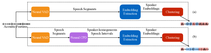
Figure 1: Illustration of the speaker diarisation system. Path (a) denotes the window-level clustering pipeline. Path (b) denotes the full pipeline with the CPD component, which leads to the speaker-homogeneous segment-level clustering results.

Given an input audio stream, VAD detects audio segments containing speech which are then further processed by the CPD component and split into speaker homogeneous segments. A speaker embedding is extracted for each of these segments using an NN model. Finally, a spectral clustering algorithm is used to group similar speaker embeddings and assign one speaker label to all segments within each group. In this paper, all components, except for the clustering algorithm based on cosine similarity, use neural networks. Alternatively, if each speech segment from VAD is split into multiple windows with the same length, speaker clustering and label assignment can be performed directly on such windows. This is referred to as window-level clustering which bypasses the CPD stage as shown in Fig. 1.

3.1 Neural VAD and CPD

The VAD and CPD models are both built as NN-based frame-level binary classifiers and described below:

• The VAD model is a DNN which consists of seven FC layers with ReLU activation functions. The key strength of the DNN structure is the use of a large input window covering 55 consecutive frames (27 on each side), which provides sufficient information for high performance speech and non-speech classification (Wang et al., 2016).

• The CPD model, as shown in Fig. 2, uses a ReLU recurrent neural network (RNN) model to encode past and future input into two separate vectors respectively which are then fused into one vector using the Hadamard product followed by a softmax FC layer classifying speaker change or non-change. By viewing the RNN output vectors as speaker representations corresponding to the past and future audio segments, the Hadamard product and the output layer can be seen as making decisions on the change of speaker identity by comparing the speaker representations before and after the current time.

  To further improve the ability of the RNN to extract speaker representations, speaker embeddings instead of raw acoustic features are used as the input to the RNN model. As shown in Fig. 2, a TDNN trained to classify the training set speakers is used to extract the frame-level d-vectors which are fed into the RNN. The whole CPD model including the TDNN, the RNN, and the output layer are then jointly trained to perform speaker change/non-change classification.

.

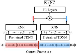
Figure 2: Proposed neural CPD structure to distinguish speaker change (C) and non-change (NC) points. The TDNN and the RNN on both sides of the current time share the same parameters. $\odot$ represents the Hadamard product.

After VAD, the original input audio stream is split into many variable length segments that may or may not contain speech, and each speech segment may have multiple speakers. Such speech segments can be directly used for speaker clustering, as shown by the dotted line in Fig. 1, or further split by the CPD model into speaker-homogeneous segments before the speaker embedding extraction and clustering stages.

3.2 Speaker embedding extraction

In this paper, Speaker embeddings, including both d-vectors and the proposed c-vectors, are the penultimate layer outputs of an NN trained to perform classification among training set speakers. In both training and test, each variable length speech segment is first split into multiple fixed-length windows with a certain amount of overlap, and a speaker embedding is then extracted from each window. At test-time, the speaker embeddings are used as input vectors to the clustering algorithm. The detailed model structures for speaker embedding extraction are presented later in Section 4.

3.3 Clustering

A modified spectral clustering (Wang et al., 2018b) approach based on the cosine distance, together with a post-processing stage, is used to cluster speaker embeddings. Spectral clustering is first performed on window-level speaker embeddings where the number of clusters is determined by the maximum eigenvalue drop-off (Luxburg, 2007), and is set to be greater than one. Next, if CPD is used, variable-length speech segments after CPD are treated as speaker-homogeneous, and each segment is assigned to a cluster whose centroid has the smallest cosine distance to the average of the window-level speaker embeddings from this segment. Otherwise, a window-level speaker-homogeneous assumption is made, and different input windows of the same speech segment are allowed to be assigned to different cluster labels. For visualisation, 2D plots using t-distributed stochastic neighbour embedding (t-SNE) for dimensionality reduction is shown in Fig. 3 where sub-figure (1) corresponds to Path (a) in Fig. 1 and and sub-figures (1), (2) and (3) together show the process of Path (b) in Fig. 1. Boundaries between two clusters are changed due to cluster assignment.

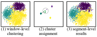
Figure 3: t-SNE 2D plots showing the clustering process of a meeting TS3004d from the AMI corpus. Each dot represents one speaker embedding extracted from a 2 second window. The three diamonds represent centroids of three clusters. Sub-figure (1) shows the window-level clustering results based on speaker embeddings, which corresponds to the results produced by Path (a) in Fig. 1. Performing the steps in sub-figures (1), (2) and (3) sequentially corresponds to the process in Path (b) in Fig. 1. Sub-figure (2) shows the procedure for cluster assignment where dots in the circle belong to the same speaker-homogeneous segment and the arrow points to the assigned cluster. A neural CPD is required to generate the speaker-homogeneous segments. Sub-figure (3) shows the clustering results at the speaker-homogeneous segment-level.

4 Combination of deep speaker embeddings

This section describes the three proposed structures to combine the window-level d-vectors for c-vector extraction using an attention mechanism, a gating mechanism, and a bilinear pooling mechanism. Window-level d-vectors are derived from multiple complementary neural network structures to obtain an enhanced speaker embedding with improved performance. A multi-head self-attentive structure with a modified penalty term is used as the temporal pooling function to derive the window-level d-vectors. Similar to the extraction procedure for d-vectors, the whole c-vector extraction model, including d-vector extraction and combination, is optimised in an end-to-end fashion to classify the training set speakers. Output vectors of the penultimate network layer are used as the c-vectors for speaker clustering.

The first structure, 2D self-attentive combination, integrates multiple window-level d-vectors into a c-vector using an extra multi-head self-attentive structure. The second structure, gated additive combination, scales each element of each window-level d-vector individually and dynamically based on the gating mechanism. Compared with the 2D self-attentive combination, the gated additive combination transforms each d-vector in a more flexible way before summing them into a combined vector. Instead of the dynamic weights used in the first two structures, bilinear pooling combination employs a separate static weight to scale the multiplicative interaction of every pair of elements from the window-level d-vectors, which enables a powerful combination method with a large number of static weights. An improved low-rank approximation with residual connections is proposed and applied to the bilinear pooling combination, in order to reduce complexity and avoid potential over-fitting issues. Lastly, a stacked structure that combines 2D self-attentive combination with bilinear pooling combination is proposed, which further leverages the complementarity of the dynamic-weight-based and static-weight-based structures.

4.1 2D self-attentive combination

The 2D self-attentive combination method, as its name suggests, extracts c-vectors by combining d-vectors in two dimensions using the multi-head self-attentive structure (Lin et al., 2017) with a modified penalty term (Sun et al., 2019). One combination dimension integrates the frame-level d-vectors extracted across time into a single window-level d-vector representing the entire window. The other combination dimension is to fuse across the window-level d-vectors produced by multiple systems.

4.1.1 Multi-head self-attentive structure

First, the multi-head self-attentive structure and the modification of the penalty term is presented. As a type of attention mechanism, the self-attentive structure dynamically calculates a set of weights, termed an annotation vector, to integrate the input sequence into one vector through a weighted average. When used to integrate the frame-level d-vectors across time, the dynamic weights in the annotation vector directly reflect the speaker-discriminative ability of the frame-level d-vectors at different time steps. To encapsulate diverse speaker characteristics, multiple annotation vectors can be generated from multiple attention output heads to combine the frame-level d-vectors using different sets of dynamic weights. The structure is “self-attentive” since the input sequence used to compute the annotation vectors is simply the sequence of frame-level d-vectors which are to be combined.

Specifically, if $\mathbf{h}(t)$ is a frame-level d-vector at time $t$, $T$ is the length of the input window, the input to the attentive structure is a $T\times N$ matrix $\mathbf{H}=[\mathbf{h}(1),\mathbf{h}(2),\dots,\mathbf{h}(T)]^{\text{T}}$, where $N$ is the size of $\mathbf{h}(t)$. Let $\mathbf{A}$ be the $T\times G$ annotation matrix formed by the $G$ annotation vectors, $\mathbf{E}$ be the $G\times N$ output matrix formed by $G$ integrated vectors, $\mathbf{A}$ and $\mathbf{E}$ can be computed by

$$\mathbf{A} =\text{Softmax}(\tanh(\mathbf{H}\mathbf{W_{1}})\mathbf{W_{2}}),$$ (1)

$$\mathbf{E} =\mathbf{A}^{\text{T}}\mathbf{H},$$ (2)

where $\text{Softmax}(\cdot)$ and $\text{tanh}(\cdot)$ refer to the softmax and hyperbolic tangent activation functions. From Eqn. (1), the attentive structure is a feedforward neural network model with two FC layers, whose weight matrices are $\mathbf{W_{1}}\in\mathbb{R}^{N\times N}$ and $\mathbf{W_{2}}\in\mathbb{R}^{N\times G}$. The input and output matrices are $\mathbf{H}$ and $\mathbf{A}$, and the softmax function is performed over each column of $\mathbf{A}$. We denote the self-attentive structure defined in Eqns. (1) and (2) as

$$\mathbf{E}=\text{SelfAtt}\left(\mathbf{h}(1),\mathbf{h}(2),\ldots,\mathbf{h}(T)\right).$$ (3)

Let $\hat{\mathbf{e}}_{g}$ be the integrated vector obtained based on the $g$ th annotation vector, and $\mathbf{E}=[\hat{\mathbf{e}}_{1},\hat{\mathbf{e}}_{2},\ldots,\hat{\mathbf{e}}_{G}]^{\text{T}}$. Let ${\mathbf{e}}$ be the window-level d-vector, ${\mathbf{e}}$ is obtained by vectorising $\mathbf{E}^{\text{T}}$, and ${\mathbf{e}}=\text{Vector}(\mathbf{E}^{\text{T}})=\text{Concat}(\hat{\mathbf{e}}_{1},\hat{\mathbf{e}}_{1},\ldots,\hat{\mathbf{e}}_{G})$ where $\text{Vector}(\cdot)$ and $\text{Concat}(\cdot)$ refer to the vectorisation and concatenation operations.

To encapsulate more diverse information in $\hat{\mathbf{e}}$ by encouraging different output heads to generate more dissimilar annotation vectors, a penalty term $\mu{\|\mathbf{A}^{\text{T}}\mathbf{A}-\mathbf{\Lambda}\|}^{2}_{\text{F}}$ can be minimised during training, where $\|\cdot\|_{\text{F}}$ denotes the Frobenius norm, $\mathbf{\Lambda}$ is a diagonal coefficient matrix, and $\mu$ is the pre-defined penalisation coefficient. Each diagonal value of $\mathbf{\Lambda}$, $\lambda_{g}=\mathbf{\Lambda}_{gg}$, controls the smoothness of the distribution of the values of the $g$ th annotation vector. The penalty term encourages different values within each annotation vector to be orthogonal and their L2-norm values to approach the corresponding smoothness coefficient $\lambda$. In the original work on self-attentive structures (Lin et al., 2017), the values of all $\lambda$ are set to 1, which results in only sparse annotation vectors with spiky values. In our previous work (Sun et al., 2019), a modified penalty term is proposed and showed that it is useful to also set some of the $\lambda$ values to be $1/G$ for extracting window-level d-vectors for diarisation, which encourages the values within the corresponding annotation vector to be more evenly distributed.

4.1.2 2D self-attentive combination

Next, the proposed 2D self-attentive combination is presented. As illustrated in Fig. 4, in order to combine $K$ window-level d-vector extraction systems, a multi-head self-attentive structure is first used to generate the window-level d-vector for each system separately, and an additional multi-head self-attentive structure is then used to fuse different window-level d-vectors across systems.

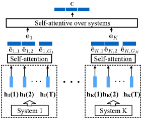
Figure 4: A sketch map of the 2D self-attentive combination applied to $K$ window-level d-vector extraction systems.

Two different methods for 2D self-attentive combination are investigated, which differ in the input of the additional self-attentive structure for window-level d-vector combination.

• First, the same dynamic weight can be assigned to the integrated vectors derived from every output head of the same extraction system. That is,

  $$\mathbf{C}=\text{SelfAtt}\left(\mathbf{W}_{1}{\mathbf{e}}_{1},\mathbf{W}_{2}{\mathbf{e}}_{2}\dots,\mathbf{W}_{K}{\mathbf{e}}_{K}\right),$$ (4)

  where ${\mathbf{e}}_{k}$ is the d-vector relevant to the $k$ th extraction system. $\mathbf{W}_{k}$ is a weight matrix used to permute the orders of components, in case that the d-vectors extracted by different pre-trained systems may not have the most suitably ordered vector components to be combined by the weighted sum of the attention mechanism.

• Alternatively, a different dynamic weight can be assigned to every integrated vector. That is,

  $$\mathbf{C}=\text{SelfAtt}\big{(}\mathbf{W}_{1}\hat{\mathbf{e}}_{1,1},\mathbf{W}_{1}\hat{\mathbf{e}}_{1,2},\dots,\mathbf{W}_{K}\hat{\mathbf{e}}_{K,G_{K}}\big{)},$$ (5)

  where $\hat{\mathbf{e}}_{k,g}$ and $G_{k}$ are the integrated vector related to the $g$ th output head and the number of output heads of the $k$ th system respectively. It is clear that this method allows different systems to have different numbers of output heads.

In both Eqns. (4) and (5), the c-vector, $\mathbf{c}$, is obtained as the vectorised version of $\mathbf{C}$.

Moreover, a baseline d-vector combination method is also introduced here. It first concatenates different d-vectors and then transforms the resulted vector with a ReLU FC layer

$$\mathbf{c} =\text{ReLU}\big{(}\mathbf{W}\,\text{Concat}({\mathbf{e}}_{1},{\mathbf{e}}_{2},\dots,{\mathbf{e}}_{K})+\mathbf{b}\big{)},$$ (6)

where $\mathbf{W}$ and $\mathbf{b}$ are the weight matrix and the bias vector of the FC layer.

4.2 Gated additive combination

The proposed gated additive combination structure relies on the gating mechanism as illustrated in Fig 5. Compared to the 2D self-attentive combination which scales all elements in each window-level d-vector by the same dynamic weight, gated additive combination allows each element in each candidate vector to be scaled with a different dynamic weight, before combination via vector addition.

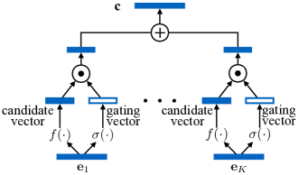
Figure 5: A sketch map of the gated additive combination for $K$ systems. $\sigma$, $\odot$, and $\oplus$ refer to the Sigmoid activation function, the Hadamard product of two vectors, and the element-wise vector addition respectively.

Analogous to an array of logic gates in electronics, in the gating mechanism (Hochreiter and Schmidhuber, 1997), a gating vector is often derived as the output vector of an FC layer with Sigmoid activation functions, whose elements are used as the dynamic weights with soft 0-1 values. Similar to the 2D self-attentive combination in Eqns. (4) and (5), a separate FC layer is used to permute the order of the elements in each window-level d-vector to generate the candidate vectors.

Specifically, a c-vector can be obtained by combining $K$ window-level d-vectors using gated additive combination as

$$\mathbf{c}=\sum\nolimits_{k=1}^{K}f\big{(}\mathbf{W}_{k}\mathbf{e}_{k}+\mathbf{b}_{w,k}\big{)}\odot\sigma\big{(}\mathbf{U}_{k}\mathbf{e}_{k}+\mathbf{b}_{u,k}\big{)},$$ (7)

where $\mathbf{W}_{k}$, $\mathbf{U}_{k}$, $\mathbf{b}_{w,k}$, and $\mathbf{b}_{u,k}$ are the weight matrices and bias vectors of the FC layers used to derive the $k$ th candidate vector and gating vector respectively. $\sigma$ and $\odot$ denote the Sigmoid activation function and Hadamard product. $f(\cdot)$ is some activation function chosen for the candidate vector.

4.3 Bilinear pooling combination

Bilinear pooling (Tenenbaum and Freeman, 2000) is a commonly used approach for fusing multimodal representations (Zhang et al., 2020), which combines two vectors using the bilinear form

$$c_{o}=\mathbf{e}_{1}^{\text{T}}\mathbf{W}_{o}\,\mathbf{e}_{2}+b_{o},$$ (8)

where $\mathbf{e}_{1}$ and $\mathbf{e}_{2}$ are the $M$-dimensional (-dim) and $N$-dim vectors to combine, and $\mathbf{W}_{o}$ and $b_{o}$ are the $M\times N$-dim weight matrix and the bias value corresponding to $c_{o}$. When generating an $O$-dim vector $\mathbf{c}=[c_{1},c_{2},\ldots,c_{O}]^{\text{T}}$ using bilinear pooling, the weight matrices $\mathbf{W}_{1},\mathbf{W}_{2},\ldots,\mathbf{W}_{O}$ form an $M\times N\times O$-dim weight tensor. It is equivalent to combining $\mathbf{e}_{1}$ and $\mathbf{e}_{2}$ using the vector outer product, and projecting the vectorisation of the resulting matrix into an $O$-dim vector space using a linear FC layer. That is,

$$\mathbf{c}=\mathbf{W}\,\text{Vector}\big{(}\mathbf{e}_{1}\otimes\mathbf{e}_{2}\big{)}+\mathbf{b},$$ (9)

where $\otimes$ is the outer product, and $\mathbf{W}$ and $\mathbf{b}$ are the $(M\times N)\times O$-dim weight matrix and bias vector of the FC layer, with $\mathbf{W}=[\text{Vector}(\mathbf{W}_{1}),\text{Vector}(\mathbf{W}_{2}),\ldots,\text{Vector}(\mathbf{W}_{O})]^{\text{T}}$. Therefore, in contrast to the attention-based and gating-based methods in Sections 4.1 and 4.2 that combine vectors in the $M$-dim or $N$-dim representation space, bilinear pooling combines two vectors by computing their outer product to capture the multiplicative interactions between all possible element pairs in a more expressive $M\times N$-dim space, which is projected to another $O$-dim vector space with $\mathbf{W}$.

Although bilinear pooling is a powerful vector combination method in theory, in practice it often suffers from issues caused by its high dimensionality (typically on the order of hundreds of thousands to a few million dimensions) that requires decomposition of the weight tensor to allow the associated parameters to be estimated properly and efficiently. Commonly used bilinear pooling decomposition methods include count sketches and convolutions (Gao et al., 2016), low-rank approximations (Kim et al., 2017), and various other tensor decomposition methods (Fukui et al., 2016; Ben-younes et al., 2017, 2019). In this section, a modified multimodal low-rank bilinear attention network (Kim et al., 2017) is proposed to combine two window-level d-vectors.

Pirsiavash et al. (2009) suggested the use of a low-rank approximation $\mathbf{W}_{o}\approx\mathbf{U}_{o1}\mathbf{U}_{o2}^{\text{T}}$ for bilinear pooling, where $\mathbf{U}_{o1}$ and $\mathbf{U}_{o2}$ are ${M\times D}$-dim and ${N\times D}$-dim matrices, and $D$ is the reduced rank of $\mathbf{W}_{o}$ which is smaller than or equal to the minimum value between $M$ and $N$. Eqn. (8) can be rewritten as $c_{o}\approx\mathbf{e}_{1}^{\text{T}}\mathbf{U}_{o1}\mathbf{U}_{o2}^{\text{T}}\,\mathbf{e}_{2}+b_{o}=\mathbf{1}^{\text{T}}(\mathbf{U}_{o1}^{\text{T}}\mathbf{e}_{1}\odot\mathbf{U}_{o2}^{\text{T}}\mathbf{e}_{2})+b_{o}$, where $\odot$ still refers to the Hadamard product and $\mathbf{1}$ is a $D$-dim vector whose elements are all set to one. Although the low-rank approximation can reduce the number of parameters, it still relies on the use of an $M\times D\times O$-dim tensor and an $N\times D\times O$-dim tensor formed by $\mathbf{U}_{11},\mathbf{U}_{21},\ldots,\mathbf{U}_{O1}$ and $\mathbf{U}_{12},\mathbf{U}_{22},\ldots,\mathbf{U}_{O2}$ respectively. To remove the use of tensors, Kim et al. (2017) proposed to tie all $\mathbf{U}_{o1}$ matrices as $\mathbf{U}_{1}$ and all $\mathbf{U}_{o2}$ matrices as $\mathbf{U}_{2}$, and a $D$-dim vector $\mathbf{p}_{o}$ is used to distinguish the value of $c_{o}$ from the other elements of $\mathbf{c}$ by $c_{o}\approx\mathbf{p}_{o}^{\text{T}}(\mathbf{U}_{1}^{\text{T}}\mathbf{e}_{1}\odot\mathbf{U}_{2}^{\text{T}}\mathbf{e}_{2})+b_{o}$. It has been also shown that using non-linear activation functions to transform the vectors before the Hadamard product can often result in better-performing models (Kim et al., 2017). Hence the initial combination of d-vectors obtained using low-rank bilinear pooling with the Hadamard product is

$$\mathbf{c}^{*}=\mathbf{P}\left(f(\mathbf{U}_{1}^{\text{T}}\mathbf{e}_{1})\odot f(\mathbf{U}_{2}^{\text{T}}\mathbf{e}_{2})\right)+\mathbf{b},$$ (10)

where $\mathbf{P}=[\mathbf{p}_{1},\mathbf{p}_{2},\ldots,\mathbf{p}_{O}]^{\text{T}}$ is an $O\times D$-dim projection matrix, $f(\cdot)$ is an activation function with a bounded range of output values, such as $\sigma(\cdot)$ and $\text{tanh}(\cdot)$. Furthermore, although a general modification of Eqn. (10) with shortcut connections was given, shortcut connections were actually not used in (Kim et al., 2017). In this paper, shortcut connections are included in bilinear pooling by using

$$\mathbf{c}=\mathbf{c}^{*}+\mathbf{V}_{1}\mathbf{e}_{1}+\mathbf{V}_{2}\mathbf{e}_{2},$$ (11)

where $\mathbf{V}_{1}$ and $\mathbf{V}_{2}$ are $O\times M$-dim and $O\times N$-dim projection matrices used to create the shortcut connections. We found in our experiments that the shortcut version of low-rank bilinear pooling given in Eqn. (11) outperformed the widely used form given in Eqn.(10).

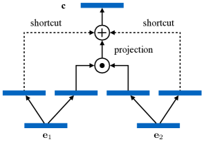
Figure 6: A sketch map of the bilinear pooling combination over two d-vector systems. $\odot$ represents the Hadamard product and $\oplus$ represents the element-wise addition of vectors.

Moreover, although bilinear pooling is only applicable for combining two vectors, a similar idea using vector outer product to combine $K$ $(K>2)$ d-vectors can be achieved by extending Eqn. (9) as

$$\mathbf{c}=\mathbf{W}\,\text{Vector}\big{(}\mathbf{e}_{1}\otimes\mathbf{e}_{2}\ldots\otimes\mathbf{(}\mathbf{e}_{K})\big{)}+\mathbf{b},$$ (12)

and Eqns. (10) and (11) can be extended similarly as

$$\mathbf{c}^{*} =\mathbf{P}\left(f(\mathbf{U}_{1}^{\text{T}}\mathbf{e}_{1})\odot f(\mathbf{U}_{2}^{\text{T}}\mathbf{e}_{2})\cdots\odot f(\mathbf{U}_{K}^{\text{T}}\mathbf{e}_{K})\right)+\mathbf{b}$$

$$\mathbf{c} =\mathbf{c}^{*}+\sum\nolimits_{k=1}^{K}\mathbf{V}_{k}\mathbf{e}_{k}.$$

4.4 Stacked combination

Lastly, a stacked combination method is proposed to exploit the use of the complementarity among different vector combination structures. There are multiple possible designs for such structures, and we only focus on those that stack any two among the three proposed combination methods.

Here we propose a structure stacking the 2D self-attentive combination and the bilinear pooling combination, which is found to perform the best in our experiments. Specifically, the two d-vectors, $\mathbf{e}_{1}$ and $\mathbf{e}_{2}$, are first combined through the first type of 2D self-attentive combination to generate the initial c-vector $\mathbf{c}^{\prime}$, and then $\mathbf{c}^{\prime}$ is fused with $\mathbf{e}_{2}$ again using the bilinear pooling to generate the final c-vector, $\mathbf{c}$. This stack of combinations is illustrated in Fig. 7.

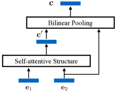
Figure 7: A sketch of the stacked combination method consists of the first type of 2D self-attentive combination and bilinear pooling combination over two d-vectors. $\mathbf{c}^{\prime}$ is the initial c-vector obtained using 2D self-attentive combination.

5 Experimental setup

5.1 Dataset details

All of the data preparation and model training was done using an extended version of HTK version 3.5.1 and PyHTK (Young et al., 2015; Zhang et al., 2019b). All systems were trained on the augmented multi-party interaction (AMI) meeting corpus. The full AMI training set contains 135 meetings with 155 speakers recorded, of which, 10% of the data for each speaker was used for held-out validation during training. The development (Dev) and evaluation (Eval) sets from the AMI official speech recognition partition were used to evaluate the performance of the proposed methods, whose details are shown in Table 1. The training set has 4–5 speakers per meeting while Dev and Eval have 4 speakers in every meeting.

Table 1: Details of the AMI official speech recognition partition.

Dataset	#Meetings	#Speakers
Train	135	155
Dev	18	21 (2 in Train)
Eval	16	16 (0 in Train)

The input features to all systems are from a 40-dim log-Mel filter bank with 25 millisecond frame size and 10 millisecond frame increment. The acoustic features were extracted from the multiple distance microphone (MDM) audio data processed by beam-forming using the BeamformIt toolkit (Anguera et al., 2005, 2007). Phase information is not included in the feature as the focus of this paper is the modelling technique (Anguera et al., 2007; Sivasankaran et al., 2018; Zheng and Zhang, 2019). Furthermore, the NIST rich transcription evaluation 2005 dataset (RT05) is used as an additional testing set, which consists of meetings with 4–10 speakers from various meeting corpora.

It is worth noting that although AMI is widely used for speaker diarisation, most studies either use different sets of meetings for testing, or the independent headset microphone audio, such as (Bullock et al., 2020; Dawalatabad et al., 2019; Pal et al., 2020a). This makes the results not comparable to those presented in this paper. Maciejewski et al. (2018); Pal et al. (2020b) used the official speech recognition data partition and MDM audio with manual segmentation. However, the SERs in their papers are not comparable to the DERs in Table 13 since the systems were trained with different training data and tested differently. Horiguchi et al. (2020) used automatic segmentation for their experiments on AMI, but the scoring procedure is different from ours since it does not include any collar.

5.2 System specifications

To extract window level d-vectors, a 2-second sliding window was applied with a 1-second overlap between adjacent windows. The TDNN and the HORNN with ReLU activation functions were chosen as two example systems for d-vector extraction and combination. The details of the TDNN structure is shown in Table 2, which resembles the one used in (Snyder et al., 2018). The HORNN system has two recurrent connections to both the previous hidden state and that 4 time steps before the current time step, which provides a simple solution to the gradient vanishing issue by using fewer parameters and calculations than LSTM. The HORNN model has 256-dim hidden states that are projected to 128-dim vectors using a shared linear projection (Zhang and Woodland, 2018). A 5 head self-attentive structure was then used for temporal pooling across the 128-dim frame-level d-vectors extracted by either a TDNN or a HORNN model. As discussed in Section 4.1.1, the $\lambda$ values for the penalty term related to each head are set to 1, 1, 1, 0.2, and 0.2. Furthermore, instead of including every frame in the 2 second window as for the TDNN model, the self-attentive structure in the HORNN model samples one frame-level d-vector for every 10 frames that considerably improves the computational efficiency without significant performance degradation. In other words, the lengths of the input sequences to the self-attentive structures of TDNN and HORNN are 200 and 20 respectively. The $640$-dim ($128\times 5$) window-level d-vectors from the TDNN and HORNN are denoted $\mathbf{e}_{\text{T}}$ and $\mathbf{e}_{\text{H}}$ and used in combination. The notation for different combination methods used in the rest of the paper are listed in Table 3.

Table 2: The structure of a TDNN model used for extracting one frame-level d-vector at time step t. The outputs from the required contexts of a layer are concatenated as the inputs to the next layer. “Layer” includes the index and the activation function of the layer, “#Frames” shows the total number of frames being used as the input when reaching that layer, and “Dimensions” gives the input dim.$\times$ output dim. of each layer.

Layer	Context	#Frames	Dimensions
1, ReLU	t-2,t-1,t,t+1,t+2	5	200 x 256
2, ReLU	t-2,t,t+2	9	768 x 256
3, ReLU	t-3,t,t+3	15	768 x 256
4, ReLU	t	15	256 x 128

Table 3: Notation and description of different combination methods for d-vectors $\mathbf{e}_{\text{T}}$ and $\mathbf{e}_{\text{H}}$.

System	Description
FCFusion$(\mathbf{e}_{\text{T}},\mathbf{e}_{\text{H}})$	FC layer combination using Eqn. (6)
SelfAtt1$(\mathbf{e}_{\text{T}},\mathbf{e}_{\text{H}})$	The first type of 2D self-attentive
	combination using Eqn. (4)
SelfAtt2$(\mathbf{e}_{\text{T}},\mathbf{e}_{\text{H}})$	The second type of 2D self-attentive
	combination using Eqn. (5)
GatedAdd$(\mathbf{e}_{\text{T}},\mathbf{e}_{\text{H}})$	Gated add. combination with Eqn. (7)
Bilinear${}_{f}(\mathbf{e}_{\text{T}},\mathbf{e}_{\text{H}})$	Bilinear pooling combination based on
	Eqn. (11) with activation function $f(\cdot)$

After the combination stage, another linear FC layer was used to project the derived c-vectors, $\mathbf{c}$, down to a 128-dim space, which was then used as the final input to the clustering algorithm. Both the TDNN and HORNN models were pre-trained in a layer-by-layer fashion without self-attentive structures. Finetuning was performed by jointly training all parameters of each window-level d-vector extraction system. When performing c-vector combination, unless explicitly stated. the combination parameters were also jointly trained with the parameters associated with the window-level d-vector extraction systems. Moreover, instead of using the standard softmax output activation function with cross-entropy loss at the output layers of the d-vector and c-vector extraction systems, the angular softmax training loss (Liu et al., 2017; Huang et al., 2018) was adopted with the $m$ factor set to $1$, to ensure that the derived embeddings are trained to discriminate speakers based on the cosine distance. This improves consistency between the performance of the speaker embeddings and the clustering results, since we use spectral clustering with the cosine distance.

5.3 Evaluation metrics

Model performance was evaluated using the diarisation error rate (DER) which is the sum of the speaker (clustering) error rate (SER), missed speech (MS) and false alarm (FA). As in training, a 2-second sliding window with 1-second overlap is applied, and 128-dim c-vectors were extracted as the output vectors from the penultimate layer. The threshold value for spectral clustering pre-processing stage is tuned on the Dev set, and directly applied to the AMI Eval set and RT05. Scoring uses the setup from the NIST rich transcription evaluations with a 0.25 second collar. If not specified, overlapped speech was not scored.

Table 4: Statistics of the original and modified reference files. “#Segments” shows the number of scored speech segments in the reference. “%Overlap” is measured by the total time of overlap speech divided by the total segmented audio time. “Time” gives the actual time after applying collars and removing overlap, and the total intra-segment non-speech time.

Reference	#Segments	%Overlap	Time (second)
Dev (Original)	13059	15.2	18613 / 7290
Dev (Modified)	17218	10.5	14973 / 3082
Eval (Original)	12612	15.3	18075 / 8241
Eval (Modified)	17100	9.6	14021 / 3134

Apart from the original manual segmentation with the official AMI release (termed as the original segmentation), we created a modified version of the manual segmentation (termed as the modified segmentation) by comparing each original manual segment with frame to speech and non-speech alignments generated by forced alignment using a pre-trained speech recognition system (Young et al., 2015). To form the modified segmentation, non-speech intervals that were longer than 0.2 seconds in the original segmentation were reduced to leave a 0.1 second collar on both ends of each segment. The manual segmentation was modified since many original manual segments had very long non-speech parts at their beginning or end, which results in many unnecessary overlapping regions and has an impact on the speaker clustering performance. The original reference was also modified accordingly to form the modified reference to match the modified segmentation.

Statistics of both the original and modified references, including the number of segments, the portion of overlapped speech, the total scored time, and the total intra-segment non-speech time are shown in Table 4. In the modified reference for the Dev and Eval sets, both the total scored time and the total intra-segment non-speech time have been reduced. Since the reduction in the total intra-segment non-speech time is larger, the amount of speech scored in the modified reference is increased, which shows the benefit of modifying the reference. Meanwhile, the total time of overlapped segments of Dev and Eval is reduced from 4,178 and 4,049 seconds to 2,535 and 2,180 seconds respectively.

6 Experimental results

6.1 AMI Results with Manual Segmentation

This section gives the results of experiments performed on the AMI data using the manual segmentation without using the VAD and CPD stages. It directly compares the speaker clustering performance with different model structures for speaker embedding extraction.

Table 5: AMI results in %SER of different model combination methods on the manual segmentation. “Original” and “Modified” refer to the results obtained by testing on the original and modified segmentation and scored against the original and modified reference files accordingly. “#Params.” shows the number of parameters in each combination structure, and “Classification Accuracy” is the speaker classification accuracy on the held-out validation set. “Manual selection per meeting” is an oracle system obtained by manually switching between the TDNN and HORNN systems according to their %SERs on Dev or Eval separately.

System	#Params	Classification	Original		Modified
	(million)	accuracy (%)	Dev	Eval	Dev	Eval
$\mathbf{e}_{\text{T}}$ (TDNN)	0.6	77.6	14.3	15.4	19.8	15.4
$\mathbf{e}_{\text{H}}$ (HORNN)	0.2	74.1	13.2	15.4	13.6	15.9
FCFusion$(\mathbf{e}_{\text{T}},\mathbf{e}_{\text{H}})$	1.0	76.4	12.8	14.7	13.5	15.2
SelfAtt1$(\mathbf{e}_{\text{T}},\mathbf{e}_{\text{H}})$	0.8	79.1	12.1	14.1	11.5	14.5
SelfAtt2$(\mathbf{e}_{\text{T}},\mathbf{e}_{\text{H}})$	0.8	78.6	12.0	13.1	11.8	13.9
GatedAdd$(\mathbf{e}_{\text{T}},\mathbf{e}_{\text{H}})$	1.0	80.0	12.8	12.3	12.1	11.7
Bilinear${}_{\sigma}(\mathbf{e}_{\text{T}},\mathbf{e}_{\text{H}})$	1.0	80.7	11.6	12.9	11.9	14.2
Bilinear${}_{\text{tanh}}(\mathbf{e}_{\text{T}},\mathbf{e}_{\text{H}})$	1.0	80.6	12.2	13.6	12.9	13.9
Bilinear${}_{\sigma}(\text{SelfAtt1}(\mathbf{e}_{\text{T}},\mathbf{e}_{\text{H}}),\mathbf{e}_{\text{H}})$	2.2	80.6	10.6	12.0	10.7	10.5
Bilinear${}_{\text{tanh}}(\text{SelfAtt1}(\mathbf{e}_{\text{T}},\mathbf{e}_{\text{H}}),\mathbf{e}_{\text{H}})$	2.2	80.9	11.4	12.5	11.4	12.5
Manual selection per meeting	N/A	N/A	12.7	11.4	13.4	11.5

6.1.1 Analysis on the penalty term of the multi-head self-attentive structure

As discussed in Section 4.1.1 and shown in Fig. 8, $\lambda_{g}$, the self-attentive structure penalty term coefficient relevant to the $g$ th annotation vector, can determine if the dynamic weights in the annotation vector has a “spiky” or “smooth” distribution. As found in our previous work (Sun et al., 2019), mixing the “spiky” and “smooth” annotation vectors can result in better-performing speaker embeddings, and therefore is used throughout this paper.

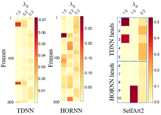
Figure 8: Heatmaps of the dynamic weights in selected annotation vectors produced by different self-attentive structures with the same input window. Left: Annotation vector values over frames that integrate frame-level d-vectors by both the TDNN and HORNN systems. Right: Annotation vector values assigned to each integrated vector $\hat{\mathbf{e}}_{k,g}$ by the second type of 2D self-attentive combination to generate a c-vector. Three annotation vectors relevant to different $\lambda_{g}$ values in the penalty term are selected from the system and shown in each plot.

Furthermore, the plot in the right part of Fig. 8 shows that the annotation vectors focus on different integrated vectors from different systems, indicating the complementarity between the example TDNN and HORNN d-vector systems.

6.1.2 SER Comparison

Next, the speaker clustering results using manual segmentation obtained using different combination methods are presented and discussed. As shown in Table 5, since the clustering threshold used for spectral clustering was determined based on Dev set performance, the Dev results are more consistent with the speaker classification accuracy on the validation set than those on Eval. The poorer TDNN performance on Dev set using the modified segmentation is due to two meetings having significantly higher SER than when using original segmentation. By comparing the results obtained with both the original and modified segmentation, apart from FCFusion$(\mathbf{e}_{\text{T}},\mathbf{e}_{\text{H}})$, all the other c-vector systems outperform both TDNN and HORNN d-vector systems. For the other c-vector systems, Bilinear${}_{\sigma}(\mathbf{e}_{\text{T}},\mathbf{e}_{\text{H}})$ gives the lowest SERs with the original segmentation but not such good results for the modified segmentation. GatedAdd$(\mathbf{e}_{\text{T}},\mathbf{e}_{\text{H}})$ produces consistently low SERs with both segmentations.

From the results in Table 5, it is clear that the systems with multiplicative combination, Bilinear${}_{\sigma}(\mathbf{e}_{\text{T}},\mathbf{e}_{\text{H}})$ and Bilinear${}_{\text{tanh}}(\mathbf{e}_{\text{T}},\mathbf{e}_{\text{H}})$, generate different and complementary outputs compared with the additive combination methods. The systems that combine the additive and multiplicative combination structures, Bilinear${}_{\sigma}(\text{SelfAtt1}(\mathbf{e}_{\text{T}},\mathbf{e}_{\text{H}}),\mathbf{e}_{\text{H}})$ and Bilinear${}_{\text{tanh}}(\text{SelfAtt1}(\mathbf{e}_{\text{T}},\mathbf{e}_{\text{H}}),\mathbf{e}_{\text{H}})$, whose structures are shown in Fig. 7, use $\sigma(\cdot)$ and $\text{tanh}(\cdot)$ as the activation function $f(\cdot)$ respectively. Bilinear${}_{\sigma}(\text{SelfAtt1}(\mathbf{e}_{\text{T}},\mathbf{e}_{\text{H}}),\mathbf{e}_{\text{H}})$ gives the lowest SERs with both types of segmentation and the performance is even better than the results obtained by manually selecting between the results obtained by the TDNN and HORNN for each meeting. The best c-vector system with overall %SERs of 11.3 and 10.6 on the original and manual segmentation outperform those given by the TDNN and HORNN d-vector systems by a considerable margin of 21% relative.

6.2 AMI and RT05 Diarisation Results

In this section, the full speaker diarisation pipeline shown in Fig. 1 is used to process both AMI and RT05. It takes each entire audio stream as the input, and outputs the speech segments along with the relevant speaker labels.

6.2.1 Window-level clustering based on VAD output

The segments obtained using VAD were evaluated against both the original reference and the modified reference, and the results are shown in Table 6.

Table 6: AMI VAD results scored using the original and modified reference files, which are presented in the form of %MS | %FA.

Dataset	Original Reference	Modified Reference
Dev	3.6 | 1.7	1.2 | 4.0
Eval	4.7 | 2.1	1.3 | 3.6

The minimum non-speech segment duration is used as a hyper-parameter during VAD to determine the segmentation. If the duration of the non-speech segment in between of two speech segments is shorter than the threshold, the non-speech segment is regarded as an intra-utterance silence and will be merged into one segment together with its surrounding speech segments. To achieve a good balance between the MS and FA obtained using the original reference, the threshold needed to be set to 1.2 seconds. The best threshold found for the modified reference is 0.2 seconds, which is a more reasonable maximum length of the intra-utterance silence showing the value of the modified reference. Therefore, in this section, only the results obtained using the modified reference are considered.

The speech segments obtained using only the VAD stage were then used to perform window-level clustering, which is more directly influenced by the c-vector performance compared to the results obtained with an extra CPD stage. The window-level speaker clustering results are shown in Table 7, which leads to conclusions similar to those obtained based on the manual segmentation results. The DER results which are shown in Table 10 can be obtained by adding each SER to the corresponding MS and FA in Table 6.

Table 7: AMI %SER results on the automatic segmentation obtained based on the VAD output. Window-level speaker clustering is used for spectral clustering. Scoring is performed against the modified reference.

System	Dev	Eval
$\mathbf{e}_{\text{T}}$ (TDNN)	17.9	18.5
$\mathbf{e}_{\text{H}}$ (HORNN)	14.6	17.7
FCFusion$(\mathbf{e}_{\text{T}},\mathbf{e}_{\text{H}})$	14.1	15.6
SelfAtt1$(\mathbf{e}_{\text{T}},\mathbf{e}_{\text{H}})$	12.4	14.9
SelfAtt2$(\mathbf{e}_{\text{T}},\mathbf{e}_{\text{H}})$	13.5	16.6
GatedAdd$(\mathbf{e}_{\text{T}},\mathbf{e}_{\text{H}})$	14.3	14.8
Bilinear${}_{\sigma}(\mathbf{e}_{\text{T}},\mathbf{e}_{\text{H}})$	12.9	13.9
Bilinear${}_{\text{tanh}}(\mathbf{e}_{\text{T}},\mathbf{e}_{\text{H}})$	14.0	13.1
Bilinear${}_{\sigma}(\text{SelfAtt1}(\mathbf{e}_{\text{T}},\mathbf{e}_{\text{H}}),\mathbf{e}_{\text{H}})$	13.6	10.7
Bilinear${}_{\text{tanh}}(\text{SelfAtt1}(\mathbf{e}_{\text{T}},\mathbf{e}_{\text{H}}),\mathbf{e}_{\text{H}})$	13.4	13.4

6.2.2 Results with additive combination methods

Table 8: Comparison among different additive combination methods. %DER is computed on both AMI Dev and Eval with 34 meetings in total. The numbers of positive and negative signs are the numbers of meetings that the relevant system performs better and worse than FCFusion$(\mathbf{e}_{\text{T}},\mathbf{e}_{\text{H}})$. Detailed meeting level results can be found in Table 14 in the Appendix.

System	Overall %DER	Sign + / -	$p$-value
FCFusion$(\mathbf{e}_{\text{T}},\mathbf{e}_{\text{H}})$	19.9%	N/A	N/A
SelfAtt1$(\mathbf{e}_{\text{T}},\mathbf{e}_{\text{H}})$	18.7%	22 / 12	0.032
GatedAdd$(\mathbf{e}_{\text{T}},\mathbf{e}_{\text{H}})$	19.6%	21 / 13	0.054

In this section, a meeting level comparison is performed among the additive combination methods: FCFusion$(\mathbf{e}_{\text{T}},\mathbf{e}_{\text{H}})$, SelfAtt1$(\mathbf{e}_{\text{T}},\mathbf{e}_{\text{H}})$, and GatedAdd$(\mathbf{e}_{\text{T}},\mathbf{e}_{\text{H}})$. Since SER varies significantly across different meetings, this comparison aims to find if the improvement is from only a few meetings that perform a lot better, or it is consistent across the majority of meetings. A sign test is performed on SelfAtt1$(\mathbf{e}_{\text{T}},\mathbf{e}_{\text{H}})$, and GatedAdd$(\mathbf{e}_{\text{T}},\mathbf{e}_{\text{H}})$, both compared to FCFusion$(\mathbf{e}_{\text{T}},\mathbf{e}_{\text{H}})$, with p-values reported.

As shown in Table 8, SelfAtt1$(\mathbf{e}_{\text{T}},\mathbf{e}_{\text{H}})$ not only achieved a lower overall DER, but also achieved better results over 22 meetings compared with FCFusion$(\mathbf{e}_{\text{T}},\mathbf{e}_{\text{H}})$, which gives a $p$-value better than the significance level of 0.05. Moreover, despite GatedAdd$(\mathbf{e}_{\text{T}},\mathbf{e}_{\text{H}})$ and FCFusion$(\mathbf{e}_{\text{T}},\mathbf{e}_{\text{H}})$ result in similar DERs, the former system achieved better performances over 21 meetings with a $p$-value close to the significance level of 0.05. The significance level confirms the consistent improvement across the majority of meetings.

6.2.3 Full pipeline results with the CPD stage

Table 9: The results of different CPD models. Collars of 0.5 second are applied to the ground-truth change points. “d-vector pretraining” refers to initialising the TDNN part of the CPD model with a TDNN frame-level d-vector extraction model. “Joint training” refers to jointly train the entire CPD model after the d-vector pre-training.

System	Precision	Recall	F1-score
KL-divergence CPD	0.17	0.33	0.22
Neural CPD	0.33	0.43	0.37
+ d-vector pre-training	0.42	0.64	0.51
+ joint training	0.50	0.68	0.57

From the full diarisation pipeline shown in Fig. 1, segments output from the VAD stage are sent to the CPD stage to generate speaker-homogeneous segments before clustering is performed. The input to the CPD stage covers a 1-second long input window centred at the current frame. If consecutive frames are classified as change points, the segment will be split at the centre frame into two speaker-homogeneous segments. After splitting, segments shorter than 0.3 second will be merged into its surrounding segments to avoid over-segmentation. The values of Precision, Recall and F1-score produced by different CPD systems are given in Table 9. The neural CPD is trained from scratch unless explicitly specified. While the neural CPD model proposed in Section 3.1 trained from scratch clearly outperforms a baseline based on Kullback–Leibler-divergence (KL-divergence) between Gaussian windows (Sinha et al., 2005; Siegler et al., 1997), a considerable improvement in the CPD performance is observed, If the TDNN part of the CPD model is pretrained as a frame-level d-vector extraction model. A further improvement can be found by performing joint training of the entire CPD model.

Table 10: AMI %DER results of different systems with the automatic segmentation obtained as the VAD output, window-level clustering results, and clustering with the neural CPD output. The results are scored against the modified segmentation.

	Dev			Eval
System	VAD	Window-level	Neural	VAD	Window-level	Neural
	output	clustering	CPD	output	clustering	CPD
$\mathbf{e}_{\text{T}}$ (TDNN)	27.7	23.1	23.0	23.5	23.4	20.5
$\mathbf{e}_{\text{H}}$ (HORNN)	22.5	19.8	18.1	25.0	22.4	19.7
FCFusion$(\mathbf{e}_{\text{T}},\mathbf{e}_{\text{H}})$	22.4	19.3	18.5	22.8	20.5	18.2
SelfAtt1$(\mathbf{e}_{\text{T}},\mathbf{e}_{\text{H}})$	21.7	17.6	16.4	23.7	19.8	18.4
SelfAtt2$(\mathbf{e}_{\text{T}},\mathbf{e}_{\text{H}})$	22.7	18.7	16.7	25.7	21.5	17.7
GatedAdd$(\mathbf{e}_{\text{T}},\mathbf{e}_{\text{H}})$	22.3	19.5	17.3	19.6	19.7	16.8
Bilinear${}_{\sigma}(\mathbf{e}_{\text{T}},\mathbf{e}_{\text{H}})$	23.3	18.1	16.9	20.6	18.6	15.6
Bilinear${}_{\text{tanh}}(\mathbf{e}_{\text{T}},\mathbf{e}_{\text{H}})$	24.1	19.2	18.1	21.9	18.0	15.9
Bilinear${}_{\sigma}(\text{SelfAtt1}(\mathbf{e}_{\text{T}},\mathbf{e}_{\text{H}}),\mathbf{e}_{\text{H}})$	21.9	18.8	16.4	20.9	15.6	15.4
Bilinear${}_{\text{tanh}}(\text{SelfAtt1}(\mathbf{e}_{\text{T}},\mathbf{e}_{\text{H}}),\mathbf{e}_{\text{H}})$	21.6	18.6	16.2	23.5	18.3	17.8

The results with different automatic segmentation are presented in Table 10. In addition to window-level clustering, another baseline clusters VAD output directly by treating each VAD segment as a single speaker segment. The DERs of all systems after CPD improved compared to the window-level clustering results, and the proposed neural CPD method improves performance in all systems on both the Dev and Eval sets. Regarding systems with a single d-vector combination method, SelfAtt1$(\mathbf{e}_{\text{T}},\mathbf{e}_{\text{H}})$ achieves the best DER on Dev, with 9% relative DER reduction compared to the HORNN d-vector system. Bilinear${}_{\sigma}(\mathbf{e}_{\text{T}},\mathbf{e}_{\text{H}})$ performs the best on Eval with 21% relative DER reduction. By using the two methods together, Bilinear${}_{\sigma}(\text{SelfAtt1}(\mathbf{e}_{\text{T}},\mathbf{e}_{\text{H}}),\mathbf{e}_{\text{H}})$ achieves the lowest DERs across the table. The relative DER reductions over the HORNN d-vector system are 10% and 22% on Dev and Eval respectively. For completeness, the influence of incorporating overlapping speech regions during scoring is shown in Table 11. For the original reference, including overlap when scoring results in a much higher increase in DER compared to the modified reference. This is mainly due to the amount of overlap caused by excessive silence in the original reference being removed in the modified reference.

Table 11: %DERs on AMI Dev and Eval of Bilinear${}_{\sigma}(\text{SelfAtt1}(\mathbf{e}_{\text{T}},\mathbf{e}_{\text{H}}),\mathbf{e}_{\text{H}})$ with the automatic segmentation with neural CPD. The results were scored against both original and modified references, with or without the overlapping regions.

Score with	Original		Modified
overlap	Dev	Eval	Dev	Eval
$\times$	18.2	18.2	16.4	15.4
$\surd$	24.9	25.4	19.4	17.8

Furthermore, the proposed methods were evaluated on the NIST RT05 data set and the results are shown in Table 12. The scoring pipeline is the same as before, which excludes overlapped speech segments. Note that the systems trained on AMI were directly used on the meetings in RT05 which were recorded at 5 different sites and 4 of them are not included in the AMI corpus. The number of speakers in each meeting also varies from 4 to 10, which makes the clustering procedure even more challenging. The systems trained and tuned on AMI were directly applied to the meetings from RT05. The MS and FA together is 2.6%, and SERs can be obtained by subtracting 2.6% from corresponding DERs in Table 12. All of the proposed c-vector systems achieved better performance than any individual d-vector system. The best performance was achieved by Bilinear${}_{\text{tanh}}(\mathbf{e}_{\text{T}},\mathbf{e}_{\text{H}})$, Bilinear${}_{\sigma}(\text{SelfAtt1}(\mathbf{e}_{\text{T}},\mathbf{e}_{\text{H}}),\mathbf{e}_{\text{H}})$, and Bilinear${}_{\text{tanh}}(\text{SelfAtt1}(\mathbf{e}_{\text{T}},\mathbf{e}_{\text{H}}),\mathbf{e}_{\text{H}})$, which each gave 15% and 12% relative reductions in SERs and DERs separately compared to the TDNN baseline system. Moreover, the consistent performance gain and similar DER numbers also reflects the robustness of the proposed systems.

Table 12: RT05 results without scoring the overlapping regions obtained using our full diarisation pipeline with the neural CPD. SERs can be obtained by subtracting MS and FA, altogether 2.6%, from corresponding DERs in Table 12

System	%DER
$\mathbf{e}_{\text{T}}$ (TDNN)	16.2
$\mathbf{e}_{\text{H}}$ (HORNN)	18.5
FCFusion$(\mathbf{e}_{\text{T}},\mathbf{e}_{\text{H}})$	19.2
SelfAtt1$(\mathbf{e}_{\text{T}},\mathbf{e}_{\text{H}})$	14.5
SelfAtt2$(\mathbf{e}_{\text{T}},\mathbf{e}_{\text{H}})$	14.7
GatedAdd$(\mathbf{e}_{\text{T}},\mathbf{e}_{\text{H}})$	16.0
Bilinear${}_{\sigma}(\mathbf{e}_{\text{T}},\mathbf{e}_{\text{H}})$	14.3
Bilinear${}_{\text{tanh}}(\mathbf{e}_{\text{T}},\mathbf{e}_{\text{H}})$	14.2
Bilinear${}_{\sigma}(\text{SelfAtt1}(\mathbf{e}_{\text{T}},\mathbf{e}_{\text{H}}),\mathbf{e}_{\text{H}})$	14.2
Bilinear${}_{\text{tanh}}(\text{SelfAtt1}(\mathbf{e}_{\text{T}},\mathbf{e}_{\text{H}}),\mathbf{e}_{\text{H}})$	14.2

6.2.4 Full pipeline results using extra training data

Finally, to show the effectiveness of the proposed combination methods on large-scale training data as suggested in (Maciejewski et al., 2018), the joint VoxCeleb (Nagran et al., 2017) and VoxCeleb2 (Chung et al., 2018b) data were used following the same data preparation pipeline in (Kreyssig and Woodland, 2020). The training data contains 2,789 hours of speech and 7,323 speakers in total. A 512-dim TDNN model and a 512-dim HORNN model were trained on the VoxCeleb data, and then were jointly optimised with combination layers on the AMI training data only. The DER results are reported in Table 13, with the same VAD and CPD models used in Table 11 and Table 12. SER results can be obtained by subtracting corresponding MS and FA values.

Table 13: %DER on AMI dev, eval and the RT05 evaluation sets without scoring the overlapping regions obtained using the full diarisation pipeline with the neural CPD. TDNN and HORNN systems were trained on the VoxCeleb 1+2 data, and fine-tuned on the AMI training data. Combination parts were only trained on the AMI training data together with individual systems.

System	Dev	Eval	RT05
$\mathbf{e}_{\text{T}}$ (TDNN)	12.6	15.6	12.9
$\mathbf{e}_{\text{H}}$ (HORNN)	13.8	16.7	13.0
FCFusion$(\mathbf{e}_{\text{T}},\mathbf{e}_{\text{H}})$	14.2	16.5	13.4
SelfAtt1$(\mathbf{e}_{\text{T}},\mathbf{e}_{\text{H}})$	12.4	15.1	11.3
SelfAtt2$(\mathbf{e}_{\text{T}},\mathbf{e}_{\text{H}})$	12.8	14.5	11.2
GatedAdd$(\mathbf{e}_{\text{T}},\mathbf{e}_{\text{H}})$	12.3	14.6	11.5
Bilinear${}_{\text{tanh}}(\mathbf{e}_{\text{T}},\mathbf{e}_{\text{H}})$	11.6	14.1	12.1
Bilinear${}_{\sigma}(\mathbf{e}_{\text{T}},\mathbf{e}_{\text{H}})$	12.1	14.2	11.6
Bilinear${}_{\text{tanh}}(\text{SelfAtt1}(\mathbf{e}_{\text{T}},\mathbf{e}_{\text{H}}),\mathbf{e}_{\text{H}})$	12.1	13.9	11.3
Bilinear${}_{\sigma}(\text{SelfAtt1}(\mathbf{e}_{\text{T}},\mathbf{e}_{\text{H}}),\mathbf{e}_{\text{H}})$	12.1	13.8	11.3

DERs on individual systems and combined systems in Table 13 improved compared to the values in Table 10 when VoxCeleb and VoxCeleb2 sets are used for training. For example, the best-performing individual system in Table 13 is the TDNN whose DERs decreased from 23.0%, 20.5% and 16.2% in Table 10 to 12.6%, 15.6% and 12.9% in Table 13 on the AMI dev, eval and RT05 sets respectively.

Although the entire combination systems were not optimised on the large-scale data, improvements were found using all combination methods. While the Bilinear${}_{\text{tanh}}(\mathbf{e}_{\text{T}},\mathbf{e}_{\text{H}})$ system performed particularly well on meeting IB4002, the best system overall was Bilinear${}_{\sigma}(\text{SelfAtt1}(\mathbf{e}_{\text{T}},\mathbf{e}_{\text{H}}),\mathbf{e}_{\text{H}})$ system, which gave rise to 7%, 17% and 16% relatiev SER reductions, and 4%, 12% and 12% relative DER reductions on the AMI dev, eval and RT05 sets respectively.

7 Conclusions

In this paper, the 2D self-attentive, gated additive, and bilinear pooling based combination methods are proposed to combine window-level d-vectors to obtain more expressive c-vector speaker embeddings. Furthermore, a complete single pass speaker diarisation pipeline with NN-based VAD and CPD components has also been introduced. By combining both feedforward and recurrent d-vector extraction systems, improvements in both SER and DER have been found using all of the proposed combination methods when compared with the single system results. Our best-performing model produced state-of-the-art speaker clustering and diarisation results by further stacking the 2D self-attentive and bilinear pooling methods, which achieved 21% relative SER reductions on AMI with both manual and automatic segmentation, and 15% relative SER reductions on RT05. SER improvements to all systems were found when VoxCeleb and VoxCeleb2 data was used for training, and 7%, 17% and 16% relative SER reductions were found on the AMI dev, eval and RT05 sets using the best combination method.

Appendix A Detailed Meeting-level results

The detailed meeting level SER results from Table 8 are presented in Table 14 which gives results of different additive combination methods.

Table 14: AMI meeting-level %SER comparison for the three additive combination methods using window-level clustering and the modified reference.

Meeting	FCFusion	SelfAtt1	GateAdd
IB4001	17.2	17.2	17.0
IB4002	23.3	23.3	23.8
IB4003	7.3	6.7	7.6
IB4004	22.2	19.0	18.1
IB4010	4.9	4.5	4.0
IB4011	4.3	4.5	3.5
ES2011a	29.4	29.2	28.5
ES2011b	31.2	12.1	12.3
ES2011c	32.8	32.0	31.8
ES2011d	26.7	25.4	24.7
IS1008a	10.0	4.3	8.8
IS1008b	2.8	2.4	1.5
IS1008c	5.2	4.8	1.3
IS1008d	4.0	4.1	4.4
TS3004a	30.0	36.3	34.6
TS3004b	9.2	8.5	26.3
TS3004c	11.1	11.0	13.4
TS3004d	27.3	13.4	28.7
EN2002a	34.5	9.1	7.3
EN2002b	14.6	14.8	15.0
EN2002c	5.7	5.7	5.2
EN2002d	15.2	14.0	14.8
ES2004a	20.5	18.3	18.5
ES2004b	5.7	5.8	5.6
ES2004c	22.9	23.1	5.5
ES2004d	34.8	34.6	38.7
IS1009a	33.8	44.4	48.3
IS1009b	5.8	5.0	5.1
IS1009c	3.8	3.6	3.7
IS1009d	17.5	18.4	16.8
TS3003a	49.3	36.0	40.6
TS3003b	10.5	10.7	13.3
TS3003c	13.8	14.1	14.1
TS3003d	18.3	18.7	35.5

References

- Akira-Miasato Filho et al. (2018) Akira-Miasato Filho, V., Silva, D., Cuozzo, L., 2018. Joint discriminative embedding learning, speech activity and overlap detection for the DIHARD speaker diarization challenge, in: Proceedings of the 19th Conference of the International Speech Communication Association (Interspeech), pp. 2818–2822.
- Anguera et al. (2012) Anguera, X., Bozonnet, S., Evans, N., Fredouille, C., Friedland, G., Vinyals, O., 2012. Speaker diarization: A review of recent research. IEEE Transactions on Audio, Speech, and Language Processing 20(2), 356–370.
- Anguera et al. (2005) Anguera, X., Woofers, C., Hernando, J., 2005. Speaker diarization for multi-party meetings using acoustic fusion, in: Proceedings of the 5th IEEE Workshop on Automatic Speech Recognition and Understanding (ASRU), pp. 426–431.
- Anguera et al. (2007) Anguera, X., Wooters, C., Hernando, J., 2007. Acoustic beamforming for speaker diarization of meetings. IEEE Transactions on Audio, Speech and Language Processing 15(7), 2011–2022.
- Barras et al. (2006) Barras, C., Zhu, X., Meignier, S., Gauvain, J.L., 2006. Multistage speaker diarization of broadcast news. IEEE Transactions on Audio, Speech, and Language Processing 14(5), 1505–1512.
- Ben-younes et al. (2017) Ben-younes, H., Cadene, R., Cord, M., Thome, N., 2017. MUTAN: Multimodal Tucker fusion for visual question answering, in: Proceedings of the 17th IEEE International Conference on Computer Vision, pp. 2631–2639.
- Ben-younes et al. (2019) Ben-younes, H., Cadene, R., Thome, N., Cord, M., 2019. BLOCK: Bilinear superdiagonal fusion for visual question answering and visual relationship detection, in: Proceedings of the 33rd AAAI Conference on Artificial Intelligence (AAAI), pp. 8102–8109.
- Bhattacharya et al. (2018) Bhattacharya, G., Alam, M., Gupta, V., Kenny, P., 2018. Deeply fused speaker embeddings for text-independent speaker verification., in: Proceedings of the 19th Conference of the International Speech Communication Association (Interspeech), pp. 3588–3592.
- Bullock et al. (2020) Bullock, L., Bredin, H., Garcia-Perera, L., 2020. Overlap-aware diarization: Resegmentation using neural end-to-end overlapped speech detection, in: Proceedings of the 45th IEEE International Conference on Acoustics, Speech and Signal Processing (ICASSP), pp. 7114–7118.
- Castaldo et al. (2008) Castaldo, F., Colibro, D., Dalmasso, E., Laface, P., Vair, C., 2008. Stream-based speaker segmentation using speaker factors and eigenvoices, in: Proceedings of the 33rd IEEE International Conference on Acoustics, Speech and Signal Processing (ICASSP), pp. 4133–4136.
- Cettolo et al. (2005) Cettolo, M., Vescovi, M., Rizzi, R., 2005. Evaluation of BIC-based algorithms for audio segmentation. Computer Speech and Language 19(2), 147–170.
- Chen et al. (2019) Chen, C., Zhang, S., Yeh, C., Wang, J., Wang, T., Huang, C., 2019. Speaker characterization using TDNN-LSTM based speaker embedding, in: Proceedings of the 44th IEEE International Conference on Acoustics, Speech and Signal Processing (ICASSP), pp. 6211–6215.
- Chen and Gopalakrishnan (1998) Chen, S., Gopalakrishnan, P., 1998. Speaker, environment and channel change detection and clustering via the Bayesian information criterion, in: Proceedings of the DARPA Broadcast News Transcription and Understanding Workshop, pp. 1–6.
- Chowdhury et al. (2018) Chowdhury, F., Wang, Q., Moreno, I., , Wan, L., 2018. Attention-based models for text-dependent speaker verification, in: Proceedings of the 43rd IEEE International Conference on Acoustics, Speech and Signal Processing (ICASSP), pp. 5359–5363.
- Chung et al. (2018a) Chung, J., Nagrani, A., Zisserman, A., 2018a. VoxCeleb2: Deep speaker recognition, in: Proceedings of the 19th Conference of the International Speech Communication Association (Interspeech), pp. 1086–1090.
- Chung et al. (2018b) Chung, J.S., Nagran, A., Zisserman, A., 2018b. Voxceleb2: Deep speaker recognition, in: Proceedings of the 19th Conference of the International Speech Communication Association (Interspeech).
- Cui et al. (2017) Cui, X., Goel, V., Saon, G., 2017. Embedding-based speaker adaptive training of deep neural networks, in: Proc. Interspeech.
- Cyrta et al. (2017) Cyrta, P., Trzcinski, T., Stokowiec, W., 2017. Speaker diarization using deep recurrent convolutional neural networks for speaker embeddings. arXiv preprint arXiv:1708.02840.
- Dawalatabad et al. (2019) Dawalatabad, N., Madikeri, S., Sekhar, C., Murthy, H., 2019. Incremental transfer learning in two-pass information bottleneck based speaker diarization system for meetings, in: Proceedings of the 44th IEEE International Conference on Acoustics, Speech and Signal Processing (ICASSP), pp. 6291--6295.
- Dehak et al. (2011) Dehak, N., Kenny, P., Dehak, R., Dumouchel, P., Ouellet, P., 2011. Front-end factor analysis for speaker verification. IEEE Transactions on Audio, Speech and Language Processing 19(4), 788--798.
- Deng et al. (2019) Deng, J., Guo, J., Xue, N., Zafeiriou, S., 2019. ArcFace: Additive angular margin loss for deep face recognition, in: Proceedings of the 32nd IEEE Conference on Computer Vision and Pattern Recognition (CVPR), pp. 4685--4694.
- Diez et al. (2019) Diez, M., Burget, L., Wang, S., Rohdin, J., Černockỳ, J., 2019. Bayesian HMM based x-vector clustering for speaker diarization. Proceedings of the 20th Conference of the International Speech Communication Association (Interspeech) , 346--350.
- Fathullah et al. (2020) Fathullah, Y., Zhang, C., Woodland, P., 2020. Improved large-margin softmax loss for speaker diarisation, in: Proceedings of the 45th IEEE International Conference on Acoustics, Speech and Signal Processing (ICASSP), pp. 7104--7108.
- Ferras et al. (2016) Ferras, M., Madikeri, S., Motlicek, P., Bourlard, H., 2016. System fusion and speaker linking for longitudinal diarization of TV shows, in: Proceedings of the 41st IEEE International Conference on Acoustics, Speech and Signal Processing (ICASSP), pp. 5495--5499.
- Fox et al. (2011) Fox, E., Sudderth, E., Jordan, M., Willsky, A., 2011. A sticky HDP-HMM with application to speaker diarization. The Annals of Applied Statistics 5(2A), 1020--1056.
- Fu et al. (2019) Fu, R., Tao, J., Wen, Z., Zheng, Y., 2019. Phoneme dependent speaker embedding and model factorization for multi-speaker speech synthesis and adaptation, in: Proc. ICASSP.
- Fujita et al. (2019) Fujita, Y., Kanda, N., Horiguchi, S., Nagamatsu, K., Watanabe, S., 2019. End-to-end neural speaker diarization with permutation-free objectives. arXiv preprint arXiv:1909.05952.
- Fukui et al. (2016) Fukui, A., Park, D., Yang, D., Rohrbach, A., Darrell, T., Rohrbach, M., 2016. Multimodal compact bilinear pooling for visual question answering and visual grounding, in: Proceedings of the 2016 Conference on Empirical Methods in Natural Language Processing (EMNLP), pp. 457--468.
- Gales (2000) Gales, M., 2000. Cluster adaptive training of hidden Markov models. IEEE Transactions on Speech and Audio Processing 8(4), 417--428.
- Gao et al. (2016) Gao, Y., Beijbom, O., Zhang, N., Darrell, T., 2016. Compact bilinear pooling, in: Proceedings of the 29th IEEE Conference on Computer Vision and Pattern Recognition (CVPR), pp. 317--326.
- Garcia-Romero and Espy-Wilson (2011) Garcia-Romero, D., Espy-Wilson, C.Y., 2011. Analysis of i-vector length normalization in speaker recognition systems, in: Proceedings of the 12th Conference of the International Speech Communication Association (Interspeech), pp. 249--252.
- Garcia-Romero et al. (2017) Garcia-Romero, D., Snyder, D., Sell, G., Povey, D., McCree, A., 2017. Speaker diarization using deep neural network embeddings, in: Proceedings of the 42nd IEEE International Conference on Acoustics, Speech and Signal Processing (ICASSP), pp. 4930--4934.
- Gupta (2015) Gupta, V., 2015. Speaker change point detection using deep neural nets, in: Proceedings of the 40th IEEE International Conference on Acoustics, Speech and Signal Processing (ICASSP), pp. 4420--4424.
- Heigold et al. (2016) Heigold, G., Moreno, I., Bengio, S., Shazeer, N., 2016. End-to-end text-dependent speaker verification, in: Proceedings of the 41st IEEE International Conference on Acoustics, Speech and Signal Processing (ICASSP), pp. 5115--5119.
- Hinton et al. (2012) Hinton, G., Deng, L., Yu, D., Dahl, G., Mohamed, A.r., Jaitly, N., Senior, A., Vanhoucke, V., Nguyen, P., Sainath, T., Kingsbury, B., 2012. Deep neural networks for acoustic modeling in speech recognition: The shared views of four research groups. Journal of Selected Topics in Signal Processing 29(6), 82--97.
- Hochreiter and Schmidhuber (1997) Hochreiter, S., Schmidhuber, J., 1997. Long short-term memory. Neural Computation 9(8), 1735--1780.
- Horiguchi et al. (2020) Horiguchi, S., Garcia, P., Fujita, Y., Watanabe, S., Nagamatsu, K., 2020. End-to-end speaker diarization as post-processing. arXiv preprint arXiv:2012.10055.
- Hruz and Zajic (2017) Hruz, M., Zajic, Z., 2017. Convolutional neural network for speaker change detection in telephone speaker diarization system, in: Proceedings of the 42nd IEEE International Conference on Acoustics, Speech and Signal Processing (ICASSP), pp. 4945--4949.
- Huang et al. (2018) Huang, Z., Wang, S., Yu, K., 2018. Angular softmax for short-duration text-independent speaker verification, in: Proceedings of the 19th Conference of the International Speech Communication Association (Interspeech), pp. 3623--3627.
- Hughes and Mierle (2013) Hughes, T., Mierle, K., 2013. Recurrent neural networks for voice activity detection, in: Proceedings of the 38th IEEE International Conference on Acoustics, Speech and Signal Processing (ICASSP), pp. 7378--7382.
- India and Hernando (2017) India, M. Fonollosa, J., Hernando, J., 2017. LSTM neural network-based speaker segmentation using acoustic and language modelling, in: Proceedings of the 18th Conference of the International Speech Communication Association (Interspeech), pp. 2834--2838.
- Kenny et al. (2010) Kenny, P., Reynolds, D., Castaldo, F., 2010. Diarization of telephone conversations using factor analysis. Journal of Selected Topics in Signal Processing 4(6), 1059--1070.
- Kim et al. (2017) Kim, J.H., On, K.W., Lim, W., Kim, J., Ha, J.W., Zhang, B.T., 2017. Hadamard product for low-rank bilinear pooling, in: Proceedings of the 5th International Conference on Learning Representations (ICLR), pp. 1--14.
- Kreyssig and Woodland (2020) Kreyssig, F.L., Woodland, P.C., 2020. Cosine-distance virtual adversarial training for semi-supervised speaker-discriminative acoustic embeddings, in: Proceedings of the 21st Conference of the International Speech Communication Association (Interspeech).
- Li et al. (2021) Li, Q., Kreyssig, F., Zhang, C., Woodland, P., 2021. Discriminative neural clustering for speaker diarisation, in: Proceedings of the 8th IEEE Spoken Language Technology Workshop (SLT).
- Lin et al. (2019) Lin, Q., Yin, R., Li, M., Bredin, H., Barras, C., 2019. LSTM based similarity measurement with spectral clustering for speaker diarization. arXiv preprint arXiv:1907.10393.
- Lin et al. (2017) Lin, Z., Feng, M., dos Santos, C., Yu, M., Xiang, B., Zhou, B., Bengio, Y., 2017. A structured self-attentive sentence embedding, in: Proceedings of the 5th International Conference on Learning Representations (ICLR), pp. 1--15.
- Liu et al. (2017) Liu, W., Wen, Y., Yu, Z., Li, M., Raj, B., Song, L., 2017. SphereFace: Deep hypersphere embedding for face recognition, in: Proceedings of the 30th IEEE Conference on Computer Vision and Pattern Recognition (CVPR), pp. 212--220.
- Liu et al. (2019) Liu, Y., He, L., Liu, J., 2019. Large margin softmax loss for speaker verification, in: Proceedings of the 20th Conference of the International Speech Communication Association (Interspeech), pp. 2873--2877.
- Luxburg (2007) Luxburg, U.v., 2007. A tutorial on spectral clustering. Statistics and Computing 17, 395--416.
- Maciejewski et al. (2018) Maciejewski, M., Snyder, D., Manohar, V., Dehak, N., Khudanpur, S., 2018. Characterizing performance of speaker diarization systems on far-field speech using standard methods, in: Proceedings of the 43rd IEEE International Conference on Acoustics, Speech and Signal Processing (ICASSP), pp. 5244--5248.
- Malegaonkar et al. (2007) Malegaonkar, A., Ariyaeeinia, A., Sivakumaran, P., 2007. Efficient speaker change detection using adapted Gaussian mixture models. IEEE Transactions on Audio, Speech and Language Processing 15(6), 1859--1869.
- Meignier et al. (2006) Meignier, S., Moraru, D., Fredouille, C., Bonastre, J.F., Besacier, L., 2006. Step-by-step and integrated approaches in broadcast news speaker diarization. Computer Speech and Language 20(2-3), 303--330.
- Milner and Hain (2016) Milner, R., Hain, T., 2016. DNN-based speaker clustering for speaker diarisation, in: Proceedings of the 17th Conference of the International Speech Communication Association (Interspeech), pp. 2185--2189.
- Nagran et al. (2017) Nagran, A., Chung, J.S., Zisserman, A., 2017. Voxceleb: a large-scale speaker identification dataset, in: Proceedings of the 18th Conference of the International Speech Communication Association (Interspeech).
- Narayanaswamy et al. (2019) Narayanaswamy, V., Thiagarajan, J., Song, H., Spanias, A., 2019. Designing an effective metric learning pipeline for speaker diarization, in: Proceedings of the 44th IEEE International Conference on Acoustics, Speech and Signal Processing (ICASSP), pp. 5806--5810.
- Nguyen et al. (2009) Nguyen, T., Sun, H., Zhao, S., Khine, S., Tran, H., Ma, T., Ma, B., Chng, E., Li, H., 2009. The IIR-NTU speaker diarization systems, in: Proceedings of the RT’09, NIST Rich Transcription Workshop.
- Ning et al. (2006) Ning, H., Liu, M., Tang, H., Huang, T., 2006. A spectral clustering approach to speaker diarization, in: Proceedings of the 7th Conference of the International Speech Communication Association (Interspeech), pp. 921--924.
- Okabe et al. (2018) Okabe, K., Koshinaka, T., Shinoda, K., 2018. Attentive statistics pooling for deep speaker embedding. arXiv preprint arXiv:1803.10963.
- Pal et al. (2020a) Pal, M., Kumar, M., Peri, R., Park, T., Kim, S., Lord, C., Bishop, S., Narayanan, S., 2020a. Meta-learning with latent space clustering in generative adversarial network for speaker diarization. arXiv preprint arXiv:2007.09635.
- Pal et al. (2020b) Pal, M., Kumar, M., Peri, R., Park, T., Kim, S., Lord, C., Bishop, S., Narayanan, S., 2020b. Speaker diarization using latent space clustering in generative adversarial network, in: Proceedings of the 45th IEEE International Conference on Acoustics, Speech and Signal Processing (ICASSP), pp. 6504--6508.
- Park and Georgy (2018) Park, T., Georgy, P., 2018. Multistream diarization fusion using the minimum variance Bayesian information criterion, in: Proceedings of the 43rd IEEE International Conference on Acoustics, Speech and Signal Processing (ICASSP), pp. 5224--5228.
- Peddinti et al. (2015) Peddinti, V., Povey, D., Khudanpur, S., 2015. A time delay neural network architecture for efficient modeling of long temporal contexts, in: Proceedings of the 16th Conference of the International Speech Communication Association (Interspeech), pp. 3214--3218.
- Pirsiavash et al. (2009) Pirsiavash, H., Ramanan, D., Fowlkes, C., 2009. Bilinear classifiers for visual recognition, in: Advances in Neural Information Processing Systems 22 (NIPS), pp. 1--9.
- Prazak and Silovsky (2011) Prazak, J., Silovsky, J., 2011. Speaker diarization using PLDA-based speaker clustering, in: Proceedings of the 6th IEEE International Conference on Intelligent Data Acquisition and Advanced Computing Systems (IDAACS), pp. 347--350.
- Savoji (1989) Savoji, M., 1989. Arobust algorithm for accurate endpointing of speech signals. Speech Communication 8(1), 45--60.
- Sell and Garcia-Romero (2014) Sell, G., Garcia-Romero, D., 2014. Speaker diarization with PLDA i-vector scoring and unsupervised calibration, in: Proceedings of the 5th IEEE Spoken Language Technology Workshop (SLT), pp. 413--417.
- Sell and Garcia-Romero (2015) Sell, G., Garcia-Romero, D., 2015. Diarization resegmentation in the factor analysis subspace, in: Proceedings of the 40th IEEE International Conference on Acoustics, Speech and Signal Processing (ICASSP), pp. 4794--4798.
- Senior and Lopez-Moreno (2014) Senior, A., Lopez-Moreno, I., 2014. Improving DNN speaker independence with i-vector inputs, in: Proceedings of the 39th IEEE International Conference on Acoustics, Speech and Signal Processing (ICASSP), pp. 225--229.
- Senoussaoui et al. (2014) Senoussaoui, M., Kenny, P., Stafylakis, T., Dumouchel, P., 2014. A study of the cosine distance-based mean shift for telephone speech diarization. IEEE/ACM Transaction on Audio, Speech and Language Processing 22(1), 217--227.
- Shi et al. (2020) Shi, Y., Huang, Q., Hain, T., 2020. H-vectors: Utterance-level speaker embedding using a hierarchical attention model, in: Proceedings of the 45th IEEE International Conference on Acoustics, Speech and Signal Processing (ICASSP), pp. 7579--7583.
- Shum et al. (2013) Shum, S., Dehak, G., Dehak, R., Glass, J., 2013. Unsupervised methods for speaker diarization: An integrated and iterative approach. IEEE Transactions on Audio, Speech and Language Processing 21(10), 2015--2028.
- Shum et al. (2011) Shum, S., Dehak, N., Chuangsuwanich, E., Reynolds, D., Glass, K., 2011. Exploiting intra-conversation variability for speaker diarization, in: Proceedings of the 12th Conference of the International Speech Communication Association (Interspeech), pp. 945--948.
- Siegler et al. (1997) Siegler, M., Jain, U., Raj, B., Stern, R., 1997. Automatic segmentation, classification and clustering of broadcast news audio, in: Proceedings of the DARPA speech recognition workshop.
- Sinha et al. (2005) Sinha, R., Tranter, S., Gales, M., Woodland, P., 2005. The Cambridge University March 2005 speaker diarisation system, in: Proceedings of the 6th Conference of the International Speech Communication Association (Interspeech), pp. 2437--2440.
- Sivasankaran et al. (2018) Sivasankaran, S., Vincent, E., Fohr, D., 2018. Keyword-based speaker localization: Localizing a target speaker in a multi-speaker environment, in: Proceedings of the 19th Conference of the International Speech Communication Association (Interspeech), pp. 2703--2707.
- Snyder et al. (2018) Snyder, D., Garcia-Romero, D., Sell, G., Povey, D., Khudanpur, S., 2018. X-vectors: Robust DNN embeddings for speaker recognition, in: Proceedings of the 43rd IEEE International Conference on Acoustics, Speech and Signal Processing (ICASSP), pp. 5329--5333.
- Sun et al. (2019) Sun, G., Zhang, C., Woodland, P., 2019. Speaker diarisation using 2D self-attentive combination of embeddings, in: Proceedings of the 44th IEEE International Conference on Acoustics, Speech and Signal Processing (ICASSP), pp. 5801--5805.
- Tenenbaum and Freeman (2000) Tenenbaum, J., Freeman, W., 2000. Separating style and content with bilinear models. Neural computation 12(6), 1247–1283.
- Tranter et al. (2004) Tranter, S., Yu, K., Evermann, G., Woodland, P., 2004. Generating and evaluating segmentations for automatic speech recognition of conversational telephone speech, in: Proceedings of the 29th IEEE International Conference on Acoustics, Speech and Signal Processing (ICASSP), pp. 753--756.
- Variani et al. (2014) Variani, E., Lei, X., McDermott, E., Moreno, I., Gonzalez-Dominguez, J., 2014. Deep neural networks for small footprint text-dependent speaker verification, in: Proceedings of the 39th IEEE International Conference on Acoustics, Speech and Signal Processing (ICASSP), pp. 4052--4056.
- Waibel et al. (1989) Waibel, A., Hanazawa, T., Hinton, G., Shikano, K., Lang, K., 1989. Phoneme recognition using time-delay neural networks. IEEE Transactions on Acoustics, Speech, and Signal Processing 37(3), 328--339.
- Wan et al. (2018) Wan, L., Wang, Q., Papir, A., Moreno, I., 2018. Generalized end-to-end loss for speaker verification, in: Proceedings of the 43rd IEEE International Conference on Acoustics, Speech and Signal Processing (ICASSP), pp. 4879--4883.
- Wang et al. (2018a) Wang, H., Wang, Y., Zhou, Z., Ji, X., Gong, D., Zhou, J., Li, Z., Liu, W., 2018a. CosFace: Large margin cosine loss for deep face recognition, in: Proceedings of the 31st IEEE Conference on Computer Vision and Pattern Recognition (CVPR), pp. 5265--5274.
- Wang et al. (2020) Wang, J., Xiao, X., Wu, J., Ramamurthy, R., Rudzicz, F., Brudno, M., 2020. Speaker diarization with session-level speaker embedding refinement using graph neural networks, in: Proceedings of the 45th IEEE International Conference on Acoustics, Speech and Signal Processing (ICASSP), pp. 7109--7113.
- Wang et al. (2016) Wang, L., Zhang, C., Woodland, P., Gales, M., Karanasou, P., Lanchantin, P., Liu, X., Qian, Y., 2016. Improved DNN-based segmentation for multi-genre broadcast audio, in: Proceedings of the 41st IEEE International Conference on Acoustics, Speech and Signal Processing (ICASSP), pp. 5700--5704.
- Wang et al. (2018b) Wang, Q., Downey, C., Wan, L., Mansfield, P., Lopez Moreno, I., 2018b. Speaker diarization with LSTM, in: Proceedings of the 43rd IEEE International Conference on Acoustics, Speech and Signal Processing (ICASSP), pp. 5239--5243.
- Wang et al. (2018c) Wang, Q., Okabe, K., Lee, K., Yamamoto, H., Koshinaka, T., 2018c. Attention mechanism in speaker recognition: What does it learn in deep speaker embedding?, in: The 7th IEEE Spoken Language Technology Workshop, pp. 1052--1059.
- Wooters and Huijbregts (2007) Wooters, C., Huijbregts, M., 2007. The ICSI RT07s speaker diarization system, in: Proceedings of the International Evaluation Workshops CLEAR 2007 and RT 2007, pp. 509--519.
- Xie et al. (2019) Xie, J., Garcia-Perera, L., Povey, D., Khudanpur, S., 2019. Multi-PLDA diarization on children’s speech, in: Proceedings of the 20th Conference of the International Speech Communication Association (Interspeech), pp. 376--380.
- Yella and Stolcke (2015) Yella, S., Stolcke, A., 2015. A comparison of neural network feature transforms for speaker diarization, in: Proceedings of the 16th Conference of the International Speech Communication Association (Interspeech), pp. 3026--3030.
- Young et al. (2015) Young, S., Evermann, G., Gales, M., Hain, T., Kershaw, D., Liu, X., Moore, G., Odell, J., Ollason, D., Povey, D., Ragni, A., Valtchev, V., Woodland, P., Zhang, C., 2015. The HTK Book (for HTK version 3.5). Cambridge University Engineering Department.
- Yu et al. (2019) Yu, Y., Fan, L., Li, W., 2019. Ensemble additive margin softmax for speaker verification, in: Proceedings of the 44th IEEE International Conference on Acoustics, Speech and Signal Processing (ICASSP), pp. 6046--6050.
- Zhang et al. (2019a) Zhang, A., Wang, Q., Zhu, Z., Paisley, J., Wang, C., 2019a. Fully supervised speaker diarization, in: Proceedings of the 44th IEEE International Conference on Acoustics, Speech and Signal Processing (ICASSP), pp. 6301--6305.
- Zhang et al. (2019b) Zhang, C., Kreyssig, F., Li, Q., Woodland, P., 2019b. PyHTK: Python library and ASR pipelines for HTK, in: Proceedings of the 44th IEEE International Conference on Acoustics, Speech and Signal Processing (ICASSP), pp. 6470--6474.
- Zhang and Woodland (2018) Zhang, C., Woodland, P., 2018. High order recurrent neural networks for acoustic modelling, in: Proceedings of the 43rd IEEE International Conference on Acoustics, Speech and Signal Processing (ICASSP), pp. 5849--5853.
- Zhang et al. (2020) Zhang, C., Yang, Z., He, X., Deng, L., 2020. Multimodal intelligence: Representation learning, information fusion, and applications. IEEE Journal of Selected Topics in Signal Processing 14(3), 487--493.
- Zhang and Wu (2013) Zhang, X.L., Wu, J., 2013. Deep belief networks based voice activity detection. IEEE Transactions on Audio, Speech, and Language Processing 21(4), 697--710.
- Zheng and Zhang (2019) Zheng, N., Zhang, X.L., 2019. Phase-aware speech enhancement based on deep neural networks. IEEE/ACM Transactions on Audio, Speech, and Language Processing 27(1), 63--76.
- Zhu et al. (2005a) Zhu, X., Barras, C., Meignier, S., Gauvain, J.L., 2005a. Combining speaker identification and BIC for speaker diarization, in: Proceedings of the 6th Conference of the International Speech Communication Association (Interspeech), pp. 2441--2444.
- Zhu et al. (2005b) Zhu, X., Barras, C., Meignier, S., Gauvain, J.L., 2005b. Combining speaker identification and BIC for speaker diarization, in: Proceedings of the 6th Conference of the International Speech Communication Association (Interspeech), pp. 2441--2444.
- Zhu et al. (2018) Zhu, Y., Ko, T., Snyder, D., Mak, B., Povey, D., 2018. Self-attentive speaker embeddings for text-independent speaker verification, in: Proceedings of the 19th Conference of the International Speech Communication Association (Interspeech), pp. 3573--3577.