spacing=nonfrench
Patchworking Oriented Matroids
Abstract.
In a previous work, we gave a construction of (not necessarily realizable) oriented matroids from a triangulation of a product of two simplices. In this follow-up paper, we use a variant of Viro’s patchworking to derive a topological representation of the oriented matroid directly from the polyhedral structure of the triangulation, hence finding a combinatorial manifestation of patchworking besides tropical algebraic geometry. We achieve this by rephrasing the patchworking procedure as a controlled cell merging process, guided by the structure of tropical oriented matroids. A key insight is a new promising technique to show that the final cell complex is regular.
Key words and phrases:
oriented matroid, triangulation, product of simplices, tropical oriented matroid, topological representation theorem, pseudosphere arrangement, patchworking, PL-topology, poset topology, poset quotient2020 Mathematics Subject Classification:
52C40; 05E45, 14T15, 52C30, 57N60, 57Q991. Introduction
Oriented matroids are ordinary matroids equipped with extra sign data, which capture and extend the combinatorics of directed graphs, real hyperplane arrangements, and more generally linear dependence over . They appear in many subjects in mathematics and related areas, from discrete geometry and optimization algorithms to algebraic geometry and topology; we refer the reader to [5, Chapter 1 & 2] for more examples. Besides having various equivalent combinatorial axiom systems, a major result in the theory of oriented matroids is the Topological Representation Theorem of Folkman and Lawrence [12], which states that every oriented matroid can be represented by a pseudosphere arrangement (a topological generalization of real hyperplane arrangements) and vice versa.
Inspired by the work of Sturmfels and Zelevinsky on maximal minors, and connections with tropical geometry and optimization problems, the authors of the current paper introduced in [7] a construction of (uniform) oriented matroids from triangulations of with suitable sign data. While the case of regular triangulations is implicit in the literature using signed tropicalization, considering general triangulations allows us to obtain non-realizable oriented matroids, including Ringel’s classical example (see [7, Section 4.2]). The construction given in [7] expresses an oriented matroid using a chirotope, which assigns signs to the ordered bases of the underlying matroid. More precisely, by encoding the cells of the triangulations by forests of the complete bipartite graph , every basis is associated with a matching, and the sign of the basis is the sign of the matching as a permutation. However, in view of the polyhedral structure of a triangulation, it is natural to ask whether the topological realization of such oriented matroids can be related to the triangulation directly. In this paper, we provide a construction to achieve this.
To do so, we adapt the method of patchworking, which goes back to Viro in the 1980s [31]. Viro’s method has numerous applications in real algebraic geometry and tropical geometry (see the survey by Viro [32]111The title of our paper is inspired by the title of this survey.), and is related to the Gelfand–Kapranov–Zelevinsky theory [14]. The idea of (combinatorial) patchworking is that one can construct piecewise linear objects isotopic to real algebraic varieties by some “cut and paste” procedure, starting with a regular subdivision of a Newton polytope with sign data. Sturmfels used this idea in [30] to study complete intersections, where mixed subdivisions play the crucial role to derive the structure of the intersecting hypersurfaces. While the latter are focused on the study of the intersections, we deal with the whole cellular complex cut out by them.
Theorem A.
Given a fine mixed subdivision of and a sign matrix, we can construct a pseudosphere arrangement representing the oriented matroid in [7] via a patchworking procedure.
From this patchworking procedure, we implicitly derive an abstract real phase structure in the sense of [4, 27] from the interplay of the subdivision and the sign matrix. Since most works on patchworking aim to construct real algebro geometric objects, their proofs usually use tropicalization of polynomials or similar techniques. In contrast, the aforementioned non-realizable example shows that we can produce non-algebro geometric objects. This suggests that patchworking could be applied for other topological problems beyond tropicalization.
Our proof uses a combination of combinatorial and topological methods, and is loosely based on Horn’s second Topological Representation Theorem for tropical oriented matroids [18]. Roughly speaking, we show that it is possible to interpolate between the dual complex of a patchworking complex, which may be regarded as a cell decomposition of the boundary of the sphere, and a pseudosphere arrangement representing our oriented matroid. This is done by carefully “merging” cells together, ensuring at each step that the combinatorics and the topology are controlled. A similar technique was used by Hersh in her work on total positivity [17]. Actually, our results imply a “Topological Representation Theorem” for each interpolation step between Horn’s result and the result of Folkman and Lawrence.
We note the work of De Loera and Wicklin in [10] which extends and studies patchworking in dimension two giving rise to a combinatorial version of Hilbert’s Lemma. Furthermore, Itenberg and Shustin derive for dimension two in [20] that patchworking with arbitrary subdivisions produces real pseudoholomorphic curves. However, it seems not much work on patchworking with general subdivisions has been done in higher dimension before us.
The paper is organized as follows. In Section 2, we collect essential definitions and background for the central objects in this paper, as well as a summary of results from [7] which are needed in this part. Section 3 is devoted to stating the main theorem, Theorem A, and contains an illustration of the rank 3 case. Sections 4 and 5 elaborate on the two main ingredients in the proof of Theorem A, namely elimination systems and quotients of regular cell complexes. The main theorem itself is proved in Section 6. The dependencies of each of the sections on each other are shown below:
2. Background
Throughout the paper, we fix a ground set of size and a set of size . We often identify with and , hence fixing an ordering for them. We use and for signs interchangeably, and we adopt the ordering of signs. This is extended componentwise to a partial order on sign vectors. For a sign vector and a sign , we denote by the set of all indices such that .
2.1. Oriented Matroids
We refer the reader to [5] for a comprehensive survey on oriented matroids.
Definition 2.1.
A chirotope on of rank is a non-zero, alternating map that satisfies the Grassmann–Plücker (GP) relation:
For any , the expressions
either contain both a positive and a negative term, or are all zeros. Here means that we remove from the list.
By the alternating property, we can specify a chirotope by its values over all -tuples of strictly increasing elements, which are identified with -subsets of .
For the purpose of topological constructions, we switch to an alternative axiom system. We recall that the composition of two signed vectors agrees with in all positions with , and agrees with otherwise.
Definition 2.2.
A collection of sign vectors is the collection of covectors of an oriented matroid if
-
(1)
.
-
(2)
If , then .
-
(3)
If , then .
-
(4)
For any and , there exists such that , and for all for which the latter equality holds.
Example 2.3.
Let be an oriented matroid realized by the real matrix , i.e.,
The covectors of are precisely the sign patterns of the vectors in the row space of .
Finally, we give the definition of pseudosphere arrangements in the statement of the Topological Representation Theorem mentioned in the introduction.
Definition 2.4.
A pseudosphere arrangement of rank is a collection of -spheres piecewise-linearly (PL), central symmetrically embedded on together with sign data, i.e., for each , specify a positive and a negative side for the two connected components of . Furthermore, we require that for any , is also a PL sphere, and that for every other , either or is a PL sphere of codimension 1 within .
The face lattice of such an arrangement is isomorphic to the covector lattice of the oriented matroid; we again refer the reader to [5, Chapter 5] for details.
2.2. Triangulations of and Polyhedral Matching Fields
We refer the reader to [9], respectively [7, 24], for details in polyhedral geometry and matching fields. We denote the -simplex, respectively the product of a -simplex and an -simplex, by and respectively . We fix their embeddings in (respectively ) as (respectively ).
A collection of full-dimensional simplices is a triangulation of if
-
(1)
the vertices of each simplex is a subset of the vertices of ,
-
(2)
the union of all simplices in is ,
-
(3)
the intersection of any two simplices in is a common face of them.
By identifying the vertices of with the edges of the complete bipartite graph , each full-dimensional simplex satisfying (1) gives rise to a spanning tree of . A combinatorial characterization of when a collection of trees forms a triangulation is given in [1, Proposition 7.2].
Definition 2.5 ([7, Section 2.3]).
A polyhedral matching field is the collection of all -saturating matchings (those covering all nodes in ) that are subgraphs of the trees encoding a triangulation of , which consists of exactly one perfect matching between and for every -subset .
We describe another (larger) matching field induced from a triangulation, which comprises the full information of the original triangulation. We augment the ground set by a copy of to obtain a ground set of size , and we set all elements of to be smaller than all elements of . The collection contains, for every tree in , the tree on obtained from by adding an edge between and its copy for every .
Definition 2.6.
The pointed polyhedral matching field associated with a triangulation of is the collection of -saturating matchings on that are subgraphs of the trees in .
The Cayley trick [29] establishes a bijective correspondence between triangulations of and fine mixed subdivisions of the dilated simplex as follows: For each tree corresponding to a simplex in the triangulation , we form the Minkowski sum
where is the neighbourhood of an element in . The collection of these Minkowski sums tiles .
In [2], Ardila and Develin studied the dual of these mixed subdivisions as tropical pseudohyperplane arrangements, which generalizes tropical hyperplane arrangements as the dual of coherent mixed subdivisions [11]. In [18, 26], it was shown that these objects are equivalent to tropical oriented matroids, defined by purely combinatorial axioms back in [2].
2.3. Oriented Matroids from Triangulations of
We recall the results of [7] which are needed in this paper. For the rest of this paper, we fix a sign matrix and a polyhedral matching field extracted from a triangulation of . We also denote by the pointed polyhedral matching field encoding the starting triangulation, and by the sign matrix .
Using the ordering on and , we can interpret a matching as a permutation, and we define the sign of the matching by the sign of the permutation.
Theorem 2.7.
We denote the oriented matroid described by as .
Similarly, induces an oriented matroid on .
Now, we describe how to convert cells of a fine mixed subdivision of , as special subgraphs of , into a covector of (resp. ).
Definition 2.8.
[7, Definition 3.26] Given and , the sign matrix is defined as
Definition 2.9.
[7, Definition 3.27] Given a subgraph of and a sign vector , the sign vector is given by
Proposition 2.10.
[7, Proposition 3.32] Let be a subgraph of a tree in without isolated nodes in , and such that a node in is isolated only if the corresponding node in is isolated as well. Let be a sign vector whose support contains the set of non-isolated nodes of in .
Then the sign vector is a covector of .
Corollary 2.11.
[7, Corollary 3.33] For a subgraph of a tree in with no isolated node in , the sign vector is a covector of for every sign vector .
Note that the latter subgraphs are called covector pd-graphs in [7].
2.4. Poset and Lattice Quotients
The following definition is due to Hallam and Sagan [15], which proved useful in their work on factorizing characteristic polynomials of lattices. This definition turns out to be the right one for us as well.
Definition 2.12.
Let be a finite poset. An equivalence relation on the ground set of is -homogeneous provided the following condition holds: if in , then for every there exists such that in . We denote by either or the equivalence class of in .
Proposition 2.13 ([15, Lemma 5]).
Suppose is -homogeneous. Then we have a well-defined poset on the classes of defined as follows: in if and only if there exists and such that in . Equivalently, for every there exists such that in .
We call the poset the homogeneous quotient of by . We are particularly interested in homogeneous quotients which have nice factorizations in the following sense:
Definition 2.14.
A homogeneous quotient is an elementary quotient if every equivalence class of is either a singleton, or consists of exactly three elements such that and both cover in .
Definition 2.15.
We say that admits a factorization into elementary quotients if there exist posets such that is an elementary quotient of for all .
Since the following notion appears several times in this paper, we give the definition here:
Definition 2.16.
The augmented poset of a poset is the poset , where and are two additional elements such that for all .
3. Patchworking Pseudosphere Arrangements
3.1. Patchworking Pseudolines on an Example
The classical theory of patchworking states that the structure of the real zero set of a polynomial in one orthant, parameterized by , is captured for sufficiently small by the regular triangulation of its Newton polytope induced by the exponents of . Hence, one can recover the structure of the real zero set by gluing the triangulations for all orthants. This uses an appropriate assignment of signs to the vertices of the Newton polytope. By considering coherent fine mixed subdivisions, see Section 2.2, this was extended to complete intersections in [30].
We use patchworking of not-necessarily coherent fine mixed subdivisions of to derive a representation theorem for the oriented matroids induced from polyhedral matching fields. This can be seen as a generalization of the linear case of [30, Thm. 4] for generic hyperplane arrangements. While a complete intersection for generic hyperplanes would only yield one specific cell, the oriented matroid captures the information of all intersections in a generic hyperplane arrangement.
Example 3.1 is a toy example that illustrates our construction, which is generalized to larger and higher rank in this section.
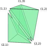
Example 3.1.
We start with the regular triangulation of induced by the height matrix
This gives rise to the following height function on the lattice points of :
Here, the height of the lattice point is the weight of the maximal matching on for which the weight function is obtained from by taking copies of the -th row of . Note that, alternatively, the latter height function of the mixed subdivision can be obtained by multiplying the -tropical linear polynomials . We refer the reader further interested in this connection to [22].
Additionally, we equip the subdivision by the sign matrix
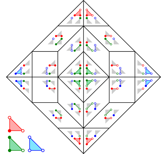
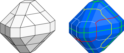
The fine mixed subdivision of induced by is shown in the upper-right quartile of Figure 2. The cells are labeled by their Minkowski summands (cf. the Cayley trick in Section 2.2) as follows. The elements of (as the three columns from left to right) are represented by the red, green, and blue simplices, respectively; the elements of (as the three rows from top to bottom) are represented by the top, lower-left, and right vertices of each simplex, respectively. Furthermore, the vertices of these simplices are labeled with signs coming from the sign matrix.
The faces of a mixed cell correspond to the subgraphs of its spanning tree without isolated nodes in . In particular, a vertex of a mixed cell can be specified by choosing a vertex from each colored simplex, thus it encodes a sign vector . Such a forest associated with a vertex is independent of the mixed cell containing it. Hence, we have a well-defined assignment of sign vectors to the vertices of the mixed subdivision. For example, the lower left vertex of the square in the upper-right quartile of Figure 2 is the Minkowski sum of a filled red vertex, an empty green and an empty blue vertex. Therefore, it encodes the sign vector .
Next we reflect the dilated simplex across the coordinate hyperplanes in so that there is a copy in every octant222We only show the upper half of that patchworking complex in Figure 2 as the construction is centrally symmetric.. We keep the same subdivision in all copies and label the vertices of these copies with sign vectors similar to the above, but instead of the original sign matrix, we negate a row of it if the corresponding coordinate in the octant is negative. For the vertex , e. g., this yields for its reflection in the upper-left quartile of Figure 2. Again, the sign vector assigned to a vertex that appears in multiple copies of the dilated simplex is independent of the copy chosen: whenever a vertex lies on a hyperplane , the -th node of must be an isolated one in the forest corresponding to the vertex, thus the negation of the -th row does not affect the sign vector.
As our example is of rank 3, we obtain a subdivision of the boundary of a dilated octahedron (which is PL homeomorphic to ), with vertices of the subdivision labeled by sign vectors.
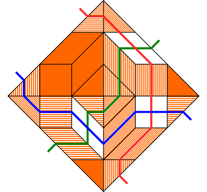
Finally, we define a “zero locus” for each element as a subset of the patchworking complex. This zero locus is dual to the cells which have a Minkowski summand with vertices of different sign. Given a cell of the subdivision, select the edges (one-dimensional faces) of the cell in which the sign vectors of their endpoints disagree on the -th coordinate, and take the convex hull of the midpoints of them. Take the union of all such convex hulls, it can be seen from Figure 3 that each of such “zero loci” is a pseudosphere on the patchworking complex.
Note that the boundary of in can be seen as the intersection with the three hyperplanes bounding the non-negative orthant. Extending these through the reflections of yields three further pseudospheres. This gives rise to an interpretation of Figure 3 as an arrangement of six pseudospheres. By ‘fattening’ the latter three coordinate pseudospheres we arrive at the extended patchworking complex introduced in the next section.
Remark 3.2.
Since oriented matroids coming from regular triangulations are all realizable, the pseudosphere arrangements constructed from a coherent fine mixed subdivision are all stretchable, which gives some non-trivial structural constraints on coherence.
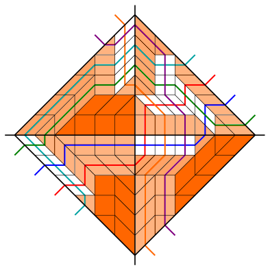
We recall the example from [7] that treats Ringel’s non-realizable uniform oriented matroid of rank on elements. It can be realized by patchworking a suitable non-coherent fine mixed subdivision of and choosing appropriate signs as depicted in Figure 4. It is not clear to the authors, if the oriented matroid can be constructed from another non-coherent fine mixed subdivision of .
It is an interesting experimental question of which of the 24 (non-isomorphic) non-realizable oriented matroids of rank on elements arise from the non-regular triangulation constructed by de Loera in [8] or its modifications by choosing appropriate signs.
Remark 3.3.
It is also an interesting problem to interpret our construction here as a limit with respect to some one-dimensional family of (meaningful) geometric objects; the regular (and non-singular) case is closely related to the theory of amoebas [25]. The rank 3 case is worth to put emphasis on, not only because it is already combinatorially rich enough, but the work of Ruberman–Starkton indicates that every pseudoline arrangement can be complexified into an arrangement of symplectic spheres [28], hence suggesting a symplectic flavored answer here (see also the aforementioned work of Itenberg–Shustin [20]).
3.2. From Fine Mixed Subdivisions to Pseudosphere Arrangements
We now state precisely our method for constructing a pseudosphere arrangement representing an oriented matroid associated to a polyhedral matching field. For this, we fix a fine mixed subdivision of . By the Cayley trick, this corresponds to a triangulation of . By means of Definition 2.6, it gives rise to a pointed polyhedral matching field on with . For an arbitrary matrix , we consider the augmented matrix as sign matrix for . Let denote the oriented matroid on associated to the pointed polyhedral matching field with the sign matrix , and let be its restriction to .
Recall from Section 2.2 that we may identify the maximal simplices in with spanning trees of . The cells of are in 1-1 correspondence with the forests contained in a spanning tree of for which for all .
We denote the cube and its polar dual, the crosspolytope, by and , respectively. For a sign vector and a set contained in the coordinate subspace of , define
Hence, denotes the reflections of to the orthant indicated by , and comprises the sign patterns of orthants containing the sign vector . For a subgraph of , let . This set encodes the unique minimal face of containing .
Proposition 3.4.
The subdivision of gives rise to the subdivision
of the boundary of , where .
We call the complex arising in the latter Proposition the extended patchworking complex; we prove the statement together with more technical properties of the extended patchworking complex in Section 6.1. This complex is analogous to the complex defined in [30, Theorem 5], with additional cells that are dual to the coordinate hyperplanes of . The extended patchworking complex subdivides the boundary of a polytope, and is therefore a PL sphere. Hence, we may consider its dual complex
The realization of the poset as a polyhedral cell complex is further explained in Section 5.1. For and , define the subcomplexes
| (2) | ||||
| (3) | ||||
Recall the notion of a pseudosphere arrangement from Definition 2.4.
Theorem 3.5.
The spaces ranging over all form an arrangement of pseudospheres within representing the oriented matroid .
Deleting the pseudospheres for yields the following.
Corollary 3.6.
The spaces ranging over all form an arrangement of pseudospheres representing the oriented matroid .
3.3. Overview of the Proof of Theorem 3.5
Before getting into the technical details of our proof, we explain the overall picture. The codimension one skeleton of in each orthant is a tropical pseudohyperplane arrangement in the sense of [2], that is, a union of PL homeomorphic images of tropical hyperplanes (codimension one skeleton of ). Including the sign data, each restricted to an orthant is either empty or is (the boundary of) a tropical (pseudo)halfspace in the sense of [21]. The latter is obtained from a tropical pseudohyperplane by removing the facets that lie between two regions of the same sign. As such, the arrangement of ’s can be thought as the end product of a facet removal process for multiple tropical pseudohyperplanes across multiple orthants.
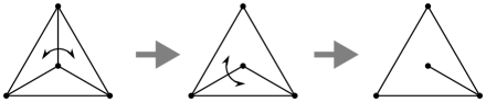
Using the results from [7] (as summarized in Section 2.3 here), we can show that the face poset of the arrangement of ’s equals the covector lattice of . The challenge now becomes topological: we need to make sure that the facet removal process does not create pathologies, so the topological structure reflects the combinatorial structure. Our approach is to formulate this process as a stepwise cell merging process, using the formalism of regular cell complexes. The removal of a facet determines an equivalence relation on the cells of the tropical pseudohyperplane arrangement: two cells are equivalent if their interiors intersect the interior of a common cell once the facet is removed. By taking the union of the cells in each equivalence class, we show that we get another regular cell complex with the same underlying topological space. Iterating this procedure, we show that we end up at a regular cell complex. Since the face poset of a regular cell complex determines the complex up to cellular homeomorphism, this completes the proof. Figure 6 depicts a two-dimensional example where naïve cell merging does not preserve regularity, hence justisfying the technical work here.
Hersh describes a similar step-by-step process in [17, §4] to simplify a regular cell complex while preserving homeomorphism type. Her single step involves collapsing a single cell to a cell on the boundary, while ours involves merging two neighbouring cells together. Thus, in some sense, her approach might be considered dual to ours.
We remark that the work in this section is very closely related to the work done by Horn in [18, Chapter 6]. Indeed, one approach to proving Theorem 3.5 is to directly use her second Topological Representation Theorem for tropical oriented matroids. Taking this approach, one would then show that the affine pseudohyperplane arrangements guaranteed by Horn’s theorem (some can be empty) glue together to form a pseudosphere arrangement, and that this pseudosphere arrangement represents the desired oriented matroid .
However, one of our goals in this paper is to furnish a proof of Theorem 3.5 that is almost entirely combinatorial. We achieve this by making use of the correspondence between tropical hyperplane arrangements and generic tropical oriented matroids, as well as the correspondence between a regular cell complex and its face poset. In particular, we show how the elimination axiom of tropical oriented matroids enables our cell merging process to work, which might lead to extensions of our method.
3.4. Relation to Real Bergman Fan and Complex
To close this section, we sketch the relation of our construction with the real Bergman fan of the oriented matroid, considered by the first author in [6, Chapter 2]. The real Bergman fan generalizes to oriented matroids the more well-known Bergman fan of a matroid, which is itself the tropical analogue of a linear subspace. In particular, the Bergman fan of a matroid is the union of cones taken over all flags of flats, whereas the real Bergman fan is the union of cones over all flags of conformal covectors:
Definition 3.7.
Let be the collection of nonzero covectors of an oriented matroid . Identify each sign vector with its associated lattice point . Then the real Bergman fan of is the collection of all cones of the form
where and each . The real Bergman complex of is the intersection of with the boundary of the hypercube .
We note that, after taking the componentwise logarithm, the real Bergman fan (resp. complex) restricted positive orthant coincides with the positive Bergman fan (resp. complex) considered by Ardila, Klivans, and Williams [3]. Conversely, the real Bergman fan can be recovered from the positive Bergman fans of all reorientations of . Such fans were used in the realizable setting by Jürgens in [23]. See [6, Chapter 2.4] for further combinatorial properties of the real Bergman fan.
The complex is a geometric realization of the order complex of . Hence, a direct consequence of the Topological Representation Theorem is that this complex is PL homeomorphic to a sphere of dimension , and its intersection with the coordinate hyperplanes of are the pseudospheres representing the elements. It is therefore natural to ask if there is a piecewise linear map from the extended patchworking complex defined in Section 3.2 to the real Bergman complex of the associated oriented matroid , one which respects the pseudosphere arrangement structure. This can indeed be carried out; we omit the details as they are routine:
Proposition 3.8.
Define the following map on the vertices of into :
Here is the matrix as in Definition 2.8, and denotes the vector of all ones. Extend this map linearly on each maximal cell of , to get a map
Then this map is well defined, and the image of this map is precisely .
Furthermore, the choices implicit in the construction of can be made so that this map respects the cellular structure of the pseudosphere arrangement over all as given by Theorem 3.5, and the pseudosphere arrangement obtained by intersecting with each of coordinate hyperplane of .
Example 3.9.
In Figure 4, the map can be visualized as contracting each shaded cell to a point, and each striped cell into a segment by contracting each stripe to a point on that segment.
4. Elimination Systems
In order to interpolate between fine mixed subdivisions and oriented matroid covectors, we consider a generalization of the set of forests arising from a fine mixed subdivision which we call an elimination system. The main result in this section is Theorem 4.12, which states that a particular poset quotient associated to an elimination system admits a factorization into elementary quotients, as defined in Section 2.4.
4.1. Elimination Systems and their posets
For a subgraph of the complete bipartite graph and , define the neighbourhood .
Definition 4.1.
Let be a collection of subsets of . Then is an elimination system provided:
-
(E1)
For each and for each , is non-empty.
-
(E2)
If and is non-empty for all , then .
-
(E3)
If and , then there exists such that and for all with .
Elimination systems are the same as generic tropical oriented matroids except without the comparability axiom; see [2, Definition 3.5].
Generalizing the face poset of the polyhedral complex of Proposition 3.4 subdividing the boundary of , we introduce a poset associated with an elimination system.
Definition 4.2.
Given an elimination system , we define the following poset:
Recall from Proposition 3.4 that denotes those such that for at least one . The ordering of the poset is given as follows: if and only if and . Recall that here means that is obtained from by setting some entries to zero. For example, ; another way to see it is that the orthant labeled by is contained in the orthant labeled by .
4.2. An Equivalence Relation of
Let be a partition of a finite set . We say that two sign vectors are equivalent (with respect to ), and write , if for all and , we have is nonempty iff is nonempty. For example, the following two sign vectors are equivalent with respect to the indicated partition of the coordinates:
This defines an equivalence relation on . We may think of each equivalence class of this equivalence relation as a sign vector in . For the above example, this would look like
Recall the construction of the sign matrix associated with a sign vector and a graph on from Definition 2.8. We introduce an equivalence relation based on the set of signs in each column of the sign matrix .
Definition 4.3.
Let be a partition of the edges of . Define the following equivalence relation on : Given and in , we say that if and with respect to the partition of given by .
Example 4.4.
Depicted below are four elements from the poset for Example 3.1. We show each element as , noting that :
Observe that these four sign vectors correspond to four full-dimensional cells in Figure 2, of which three are in the lower right orthant and the last is in the upper right orthant. They correspond to cells following the red pseudoline in Figure 3, starting from the triangle in the lower right orthant. We see right away that for as they differ in the first component. To check for the equivalence of the other three pairs, we can consider the image of the columns of to as indicated before Definition 4.3. This yields the three vectors , , . Hence, we get .
4.3. Properties of the Quotient
We assume we are given an elimination system on , and a sign matrix . We denote the poset by .
Proposition 4.5.
Suppose is covered by in . Then either and , or and .
Proof.
The fact that means that and , and either or . If , then let . Then , which means . Since , this means . Hence, is an element of such that
Since is covered by , we conclude the first inequality holds with equality, and hence and .
Otherwise, . Let . Then is not the only element of , since otherwise we would have which is forbidden by (E1). We therefore have by (E2), and hence
By covering, we conclude the second inequality holds with equality, and hence and . ∎
Corollary 4.6.
The poset is graded, with grading .∎
Given two sign vectors , define their intersection to be the sign vector such that and .
Proposition 4.7.
The augmented poset is a lattice: if have a common lower bound, then a greatest lower bound for both is given by .
Proof.
Let and be elements of with a common lower bound . Then which implies by (E2) that . Similarly, we have and so
We conclude and is a lower bound of and . The fact that and shows that is in fact a greatest lower bound, as was chosen arbitrarily.∎
Our next task is to generalize the equivalence relation on from Definition 4.3, by allowing the partition of to vary. We assume fixed a partition of which refines the partition . In terms of this partition, we say if is nonempty iff is nonempty, for all and .
Definition 4.8.
For , we say if and only if and .
Proposition 4.9.
The equivalence relation on is -homogeneous. In particular, is a poset.
Proof.
Let be two elements of , and choose . Our goal is to find such that and . Define
Thus . The definition of ensures that every sign appearing in the restricted sign vector also appears in , for all . Conversely, if and is nonzero for some , then implies there exists such that , and therefore contains the sign . Note that we are using here the fact that refines the partition . We conclude .
Observe that is nonempty for every by (E1), and since we also have is nonempty for every . Therefore, since , we have by (E2) that . Moreover, so that . We conclude . ∎
For a generalized sign vector , let count the number of nonzero coordinates in , with each counted twice. For example, if then . Note that if is the singleton partition, then is an ordinary sign vector and .
Proposition 4.10.
The poset is graded, with grading
Proof.
Fix . First note that is a maximal element in the equivalence class if and only if for all and all . Indeed, choose any . Then (E2) implies that we may find inside such that for all and all . In particular, this statement holds for the maximal elements of .
Now, for every maximal element , we have
It remains to show that respects the covering relations. Suppose that is covered by in . By homogeneity, we may choose representatives and so that is covered by in . Such an element is necessarily a maximal element of the equivalence class , which implies and for all . Since , we have , and hence and for all . It follows is maximal in . We conclude
Proposition 4.11.
The augmented poset is a lattice.
Proof.
Choose and with a common lower bound in . By homogeneity and Proposition 4.7, we may choose the representatives and so that . By homogeneity, then, is a lower bound for both and .
We show this is a greatest lower bound. Given a lower bound , we may find and such that and in . Hence, by Proposition 4.7, . Therefore, it suffices to show
For all and , we have
In particular, this shows .∎
We now come to the main theorem of this section:
Theorem 4.12.
The poset admits a factorization into elementary quotients, such that the augmented poset is a lattice for each .
Proof.
By Proposition 4.7, is a lattice. Thus, let be a partition of which refines the partition and has at least one part such that . Let , and let be the refinement of obtained by splitting the part into two parts: and . That is,
Let and denote the equivalence relations on sign vectors on induced by and , respectively. These determine -homogeneous equivalence relations and by Proposition 4.9. Let . Since is -homogeneous, and since refines , we have that is -homogeneous. Moreover, there is a natural identification . Therefore, by induction, the theorem is proved if we can show that is an elementary quotient whose augmented poset is a lattice. In fact the lattice assertion follows from Proposition 4.11.
Fix . We would like to show that the equivalence class containing in is either a singleton, or consists of exactly three elements two of which cover a third. Note that if is the zero vector, then this equivalence class is indeed a singleton. This is because we would immediately know that and , hence in this case is completely determined by .
Otherwise, the sign vector is non-zero, and in this case there are exactly three generalized sign vectors , depending on and , such that The restrictions of these to are depicted below, in all of four possible cases:
The following argument applies simultaneously to all four cases shown above. Suppose there are at least two distinct elements and in the same equivalence class of . Then there exists a unique such that
for some . We consider the three cases separately.
-
•
If or , then without loss of generality assume .
-
–
If , then by (E2) the set is in , and .
-
–
If , then by (E2) the set is in , where is the unique sign appearing in but not , and .
-
–
-
•
If , then by (E3), we can find such that
This shows . We remark that this is the only time (E3) is used.
In all three cases, we therefore have found such that . Therefore the equivalence class of in consists of the three distinct elements , , and . Their gradings in are given by, by Proposition 4.10, for . Inspecting the above four tables, we conclude that two of these elements cover the third in .∎
5. Quotients of Regular Cell Complexes
5.1. Background: Regular Cell Complexes and PL Topology
We quickly review the key aspects of combinatorial topology we wish to use. The main reference here is [5, Section 4.7].
5.1.1. Regular Cell Complexes
Definition 5.1.
A regular cell complex is a Hausdorff space together with a finite collection of balls such that:
-
(1)
The interiors of the balls in partition the space: .
-
(2)
The boundary of any is a union of members of : .
Definition 5.2.
An important special case of the above definition is a polyhedral cell complex. This is a regular cell complex such that each is a polytope in , and for each we have is a face of both and . If every polytope in is a simplex, we call a geometric simplicial complex. A triangulation of a set is a geometric simplicial complex with underlying space .
Definition 5.3.
The face poset of a regular cell complex is the poset whose underlying set is the set of balls , and whose ordering is given by inclusion.
Definition 5.4.
The order complex of a poset is the simplicial complex whose vertices are the elements of and whose simplices are the chains of . We denote by the topological space .
Proposition 5.5.
Every abstract simplicial complex (i.e. set system closed under taking subsets) can be realized as a geometric simplicial complex in some Euclidean space.
5.1.2. PL Balls and Spheres
Definition 5.6.
Given , , a map is piecewise linear (PL) if there is a triangulation of into simplices such that restricted to each simplex of is an affine function. That is, if then satisfies
for all convex combinations of the vertices of . We call a PL map that is also a homeomorphism a PL homeomorphism.
Definition 5.7.
Let be the underlying space of a polyhedral cell complex. Then is a PL -sphere (resp. PL -ball) if there is a PL homeomorphism from to the boundary of the standard -simplex (resp. to the standard -simplex).
Proposition 5.8.
-
(1)
[5, Theorem 4.7.21(i)] The union of two PL d-balls, whose intersection is a PL -ball lying in the boundary of each, is a PL -ball.
-
(2)
[5, Theorem 4.7.21(ii)] The union of two PL d-balls, which intersect along their entire boundaries, is a PL -sphere.
-
(3)
[5, Theorem 4.7.21(iii)] (Newman’s Theorem) The closure of the complement of a PL -ball embedded in a PL -sphere is itself a PL -ball.
Lemma 5.9.
Let be two PL -balls, such that is a PL -ball contained in the boundaries of both and . Then the interior of is equal to .
Proof.
By Proposition 5.8 (1), is a PL -ball. We start by showing that contains . Let . Then there is an open set containing and a homeomorphism sending to . Here denotes the ball of radius 1 in centred at the origin. Since is closed in , and since , we further have that is an open set which contains the origin; hence there exists such that the scaled open ball is contained in . It follows that is an open neighbourhood of , homeomorphic to , and entirely contained in . In particular, this means that . We conclude .
From this containment we immediately get
and in particular
Since boundaries are closed, is closed inside . Now is the boundary of in , thus it is contained in . Similarly, . By Proposition 5.8 (3), both are PL -balls with common boundary , so by Proposition 5.8 (2), is a PL -sphere contained in . Invariance of Domain implies the containment is an equality, see for example [16, Corollary 2B.4]. After taking the complement with respect to , this equality yields an expression for which simplifies to .∎
5.1.3. Regular Cell Complexes that are PL Spheres
Definition 5.10.
We say that a regular cell complex with face poset is a PL sphere if some realization of the order complex in some Euclidean space is a PL sphere.
Proposition 5.11 ([5, Proposition 4.7.26(iii)]).
Let be a regular cell complex that is a PL sphere. Then every is a PL ball.
An important fact about PL spheres is that they admit a dual cell structure:
Proposition 5.12 ([5, Proposition 4.7.26(iv)]).
Let be a regular cell complex that is a PL sphere. Then there exists a regular cell complex , also a PL sphere, such that and .
Here denotes the dual poset of . In the special case when is a polyhedral cell complex, there is a non-canonical way to construct this :
Definition 5.13.
Let be a polyhedral cell complex. A first derived subdivision is a subdivision of obtained as follows: choose a point in the relative interior of each . Then, is given by
Theorem 5.14 ([19, § 1.6]).
If is a polyhedral cell complex then may be constructed as follows: Choose a first derived subdivision of . For each cell , define
where . Then let
5.2. Quotients of Regular Cell Complexes
Our next goal is to develop a notion of a quotient of a regular cell complex , in which cells are merged together according to a given equivalence relation on the cells of .
Let be a regular cell complex with face poset , so that . Given a homogeneous quotient of , define the set
where denotes the union . Note that homogeneity of implies that as sets if and only if in .
Under certain conditions, is again a regular cell complex:
Theorem 5.15.
Suppose:
-
(1)
The poset is an elementary quotient,
-
(2)
The augmented poset is a lattice, and
-
(3)
Each is a PL ball.
Then is a regular cell complex with face poset , such that each is a PL ball.
Corollary 5.16.
Suppose admits a factorization into elementary quotients, such that is a lattice for each . Suppose further that each is a PL ball. Then is a regular cell complex with face poset .
In the remainder of this section we prove Theorem 5.15. The main ingredient is a topological criterion for to be a regular cell complex:
Lemma 5.17.
Suppose that each in is a ball whose interior equals the union of the interiors of the cells of . Then is a regular cell complex with face poset .
Proof.
We first show that is a regular cell complex. It is clear that the underlying topological spaces of and are the same. To see that the interiors of the balls in are disjoint, let and be two balls in such that
is non-empty. In particular, there must exist and such that and intersect. This can only happen if , and hence . To see that the boundary of each in is a union of members of , let be an element of . Then
| (4) |
We justify the last equality. We may write for every . Hence, the last equality holds provided we can show the following statement: whenever we have where , we must also have . The condition implies . The condition implies . On the other hand, the condition implies , and therefore . We conclude , and in particular . Note that this argument uses the fact that is a poset, which follows from homogeneity of . Now, since the interiors of cells of partition , we have by (4) that
We therefore conclude
The proof that the face poset of is is straightforward. If , then this means in particular that , hence in , hence in . Conversely, if in , then there exists a cell of contained in some cell of . By homogeneity, then, every cell of in contained in some cell of . Hence .∎
Proposition 5.18 ([5, Section 4.7, pp.204]).
Let be a regular cell complex with face poset . Then the augmented poset is a lattice if and only if is closed under non-empty intersections: for all such that is non-empty, we have .∎
Proof of Theorem 5.15.
It is clear that for any singleton class , satisfies the hypothesis of Lemma 5.17. Now suppose is a class in . It is known that the function is a rank function on . In particular, since and cover , then we must have . Moreover, since is a lattice, we must have by Proposition 5.18. Proposition 5.8 (1) and Lemma 5.9 then show that is a PL ball which satisfies the hypothesis of Lemma 5.17. ∎
6. Proof of the Main Theorem
In this section we prove Theorem 3.5. We assume the fine mixed subdivision of , the sign matrix , and the oriented matroid are as defined in Section 3.2.
6.1. Properties of the Extended Patchworking Complex
We begin this section by establishing some technical details of the extended patchworking complex defined in Section 3.2. Note that each face of the polytope is in bijection with a nonempty subset . Let denote the cells of contained in the coordinate subspace of . For and , let .
Proposition 6.1.
Define the collection of polytopes given by
Then the following statements hold:
-
(1)
is a polyhedral cell complex which subdivides the boundary of .
-
(2)
For each , both and can be recovered from .
-
(3)
For , we have if and only if and .
Remark 6.2.
The subdivision in the statement of Proposition 6.1 can be replaced by any polyhedral subdivision of .
Proof.
First note that (2) follows from the fact that each is a Minkowski sum of two affinely independent polytopes. Therefore, projection allows us to recover both and , and therefore the pair .
Recall the general fact that is a proper face of the Minkowski sum of two full-dimensional polytopes and if and only if there exists a non-zero objective function such that , where and denote the faces of and , respectively, maximized by . Specializing to the case and , we have and , where is the componentwise sign vector of , is the set of all such that , and . It follows that the collection of proper faces of is given by
Since is the union of the cells , this shows that the cells in cover the boundary of . The above fact about faces of Minkowski sums can also be used to show that the faces of are given by . This establishes (3), and that is closed under taking faces.
To establish (1), it remains to show that the intersection of two intersecting cells of is a face of both. If is non-empty, then and are conformal sign vectors since otherwise, if (say) , then would lie in the halfspace , while lies in the halfspace . Now, we would like to show , where denotes sign vector composition. As argued above, is a face of both and . Thus, it remains to show that is contained in .
Suppose , where , , , . We are done if we can show and . For this it suffices to show for all . Since are conformal, we have for all . For , we have , and hence . Thus it remains to show in the case when or .
Suppose . The fact implies , and the fact implies . Now , which implies
Hence , and so . The case is proven analogously. ∎
Recall that, by the Cayley trick, the cells in encode the simplices in , for which no node in is isolated. This directly shows that they fulfill property (E1) and (E2) of elimination systems (Definition 4.1). A proof that satisfies (E3) can be found in [26, Proposition 4.12], and this result has been generalized to arbitrary mixed subdivisions in [18, Theorem 7.11]. Hence, we conclude:
Proposition 6.3.
The set of forests encoded by form an elimination system.∎
Observing that if and only if , and that on the level of posets, taking the dual just amounts to reversing the ordering, we have
Corollary 6.4.
The map determines an isomorphism from the face poset of the dual complex to the poset defined in Definition 4.2.
6.2. The Map
We next consider the labeling of the elements of by sign vectors. For this, we use the connection between the pairs denoting cells of the extended patchworking complex and covectors established in Corollary 2.11.
Now, we look at the particular elimination system given by the fine mixed subdivision . In the following proposition, let denote the poset of non-zero covectors of . Let be the poset as in Section 4.3.
Recall from Section 4.3 the system of mixed signs . Using this as an intermediate step, one sees that the following map extending the map of Definition 2.9 is well-defined on its equivalence classes.
Definition 6.5.
Define the map by .
As we fix most of the time, we just set .
Example 6.6 (Ex. 4.4 continued).
Recall that we could identify the equivalence classes of the four sign vectors for with , , and . This shows that the images of the three equivalence classes of (as )) are the sign vectors
Note that a similar map was used in [18, §6] to prove the representation theorem for tropical oriented matroids.
Since is constant on the equivalence classes of , we just fix an element . With this, we associate the bipartite graph on having the edges of and edges between the nodes of and its copy within for each element in the support of . Now, the claim follows from Proposition 2.10.
Corollary 6.7.
For all , we have .
Proposition 6.8.
The map is a poset map.
Proof.
Suppose in . Let , and let . Then , and because , the passage from to only decreases the number of non-zero entries in each column of . However still has at least one non-zero entry in each column. From this we conclude , and therefore respects order.∎
Recall that a poset is a sphere if its order complex is a sphere; see Definition 5.4.
Theorem 6.9 (Borsuk–Ulam).
Let be posets such that both are homeomorphic to and both are equipped with a fixed-point free involutive automorphism . Let be a poset map satisfying for all . Then is surjective.
Corollary 6.10.
Assuming is a -sphere, the map is an isomorphism.
Remark 6.11.
We show that is indeed a -sphere in Section 6.4.
Proof.
For , the interpretation of as a generalized sign vector in shows that is injective. To see that is surjective, we simply note that is a fixed-point free involutive automorphism of which descends to , while is one of . Furthermore, by definition of , we have . As has rank , the poset is a -sphere by Theorem 6.12, and hence the conclusion follows from the Borsuk-Ulam Theorem.∎
6.3. Pseudosphere Arrangements from Regular Cell Complexes
The following result shows how to get pseudosphere arrangements from regular cell complexes:
Theorem 6.12 ([5, Theorem 4.3.3, Proposition 4.3.6]).
Let be an oriented matroid of rank on the ground set . Let be a regular cell complex with face poset , such that there is a poset isomorphism . Thus each cell of is labeled by some non-zero covector of . For each , define the subcomplex
Then is a -sphere, and the spaces ranging over all form an arrangement of pseudospheres within representing .
6.4. Putting it all Together
With all the pieces now in place, we are ready to prove Theorem 3.5, which asserts that our patchworking procedure yields a pseudosphere representation of .
Proof of Theorem 3.5.
As shown for Proposition 6.3, a fine mixed subdivision of gives rise to an elimination system as in Definition 4.1. Abusing notation, we denote this elimination system also by . We let be the poset of obtained by introducing signs as in Definition 4.2.
Let denotes the face poset of . By Corollary 6.4, we have . Hence the poset quotient induces a quotient . By Theorem 4.12, then, admits a factorization into elementary quotients, such that the augmented poset is a lattice for each .
As a polyhedral complex on the boundary of a -dimensional polytope, is a PL -sphere. Hence, by Proposition 5.12, is also a PL -sphere. In particular, by Proposition 5.11, each cell in is a PL ball. It follows, by Corollary 5.16, that is a regular cell complex with face poset . In particular, is a -sphere.
By Corollary 6.10, we have isomorphisms . For , define the subcomplex
of . Now, Theorem 6.12 implies that the spaces ranging over all form an arrangement of pseudospheres within representing .
It remains to show that for all , where is a subcomplex of defined in (2) and (3). For this note that the closed cells of , and hence all subcomplexes of , each consist of a union of members of . Hence, it suffices to show that for all and , we have if and only if .
For and , we have if and only if there exists such that and
As is a regular cell complex, the interiors of the balls in are disjoint, and so the above containment holds true if and only if for some such that . If , then iff . If , we have if and only if there exist such that . In either case, we conclude if and only if .∎
Acknowledgement. The first author was funded by the Deutsche Forschungsgemeinschaft (DFG, German Research Foundation) under Germany’s Excellence Strategy – The Berlin Mathematics Research Center MATH+(EXC-2046/1, project ID: 390685689). He is grateful to Josephine Yu for helpful discussions on patchworking, in particular pointing out the reference [30]. This project has received funding from the European Research Council (ERC) under the European Union’s Horizon 2020 research and innovation programme (grant agreement n° ScaleOpt-757481). The second author also thanks Xavier Allamigeon and Mateusz Skomra for inspiring discussions and Ben Smith for helpful comments. The third author was supported by Croucher Fellowship for Postdoctoral Research and Netherlands Organisation for Scientific Research Vici grant 639.033.514 during his affiliation to Brown University and University of Bern, respectively. He also thanks Cheuk Yu Mak for pointing out [28]. The second and third author both thank the Tropical Geometry, Amoebas, and Polyhedra semester program at Institut Mittag-Leffler for the introduction that started the project. The authors thank Laura Anderson and Jesus De Loera for comments on our work.
References
- [1] Federico Ardila and Sara Billey, Flag arrangements and triangulations of products of simplices, Adv. Math. 214 (2007), no. 2, 495–524.
- [2] Federico Ardila and Mike Develin, Tropical hyperplane arrangements and oriented matroids, Math. Z. 262 (2009), no. 4, 795–816.
- [3] Federico Ardila, Caroline Klivans, and Lauren Williams, The positive Bergman complex of an oriented matroid, European J. Combin. 27 (2006), no. 4, 577–591.
- [4] Benoît Bertrand, Erwan Brugallé, and Arthur Renaudineau, Haas’ theorem revisited, Épijournal Geom. Algébrique 1 (2017), Art. 9, 22.
- [5] Anders Björner, Michel Las Vergnas, Bernd Sturmfels, Neil White, and Günter M. Ziegler, Oriented matroids, Encyclopedia of Mathematics and its Applications, vol. 46, Cambridge University Press, Cambridge, 1993.
- [6] Marcel Celaya, Lattice points, oriented matroids, and zonotopes, 2019, Ph.D. Thesis, Georgia Institute of Technology.
- [7] Marcel Celaya, Georg Loho, and Chi Ho Yuen, Oriented matroids from triangulations of products of simplices, 2020, preprint arXiv:2005.01787.
- [8] J. A. de Loera, Nonregular triangulations of products of simplices, Discrete Comput. Geom. 15 (1996), no. 3, 253–264.
- [9] Jesús A. De Loera, Jörg Rambau, and Francisco Santos, Triangulations, Algorithms and Computation in Mathematics, vol. 25, Springer-Verlag, Berlin, 2010, Structures for algorithms and applications.
- [10] Jesús A. De Loera and Frederick J. Wicklin, On the need of convexity in patchworking, Adv. Appl. Math. 20 (1998), no. 2, 188–219 (English).
- [11] Mike Develin and Bernd Sturmfels, Tropical convexity, Doc. Math. 9 (2004), 1–27 (electronic), erratum ibid., pp. 205–206.
- [12] Jon Folkman and Jim Lawrence, Oriented matroids, J. Combin. Theory Ser. B 25 (1978), no. 2, 199–236.
- [13] Ewgenij Gawrilow and Michael Joswig, polymake: a framework for analyzing convex polytopes, Polytopes—combinatorics and computation (Oberwolfach, 1997), DMV Sem., vol. 29, Birkhäuser, Basel, 2000, pp. 43–73.
- [14] I. M. Gelfand, M. M. Kapranov, and A. V. Zelevinsky, Discriminants, resultants, and multidimensional determinants, Mathematics: Theory & Applications, Birkhäuser Boston, Inc., Boston, MA, 1994.
- [15] Joshua Hallam and Bruce Sagan, Factoring the characteristic polynomial of a lattice, J. Combin. Theory Ser. A 136 (2015), 39–63.
- [16] A. Hatcher, Cambridge University Press, and Cornell University. Dept. of Mathematics, Algebraic topology, Algebraic Topology, Cambridge University Press, 2002.
- [17] Patricia Hersh, Regular cell complexes in total positivity, Invent. Math. 197 (2014), no. 1, 57–114.
- [18] Silke Horn, A topological representation theorem for tropical oriented matroids, J. Combin. Theory Ser. A 142 (2016), 77–112.
- [19] J.F.P. Hudson, J.L. Shaneson, and Chicago (Ill.). University. Dept. of Mathematics, Piecewise linear topology, Mathematics lecture note series, no. Bd. 1, Department of Mathematics, University of Chicago, 1967.
- [20] Ilia Itenberg and Eugenii Shustin, Combinatorial patchworking of real pseudo-holomorphic curves, Turkish J. Math. 26 (2002), no. 1, 27–51.
- [21] Michael Joswig, Tropical halfspaces, Combinatorial and computational geometry, Math. Sci. Res. Inst. Publ., vol. 52, Cambridge Univ. Press, Cambridge, 2005, pp. 409–431.
- [22] by same author, Essentials of tropical combinatorics, in preparation.
- [23] Christian Jürgens, Real tropical singularities and Bergman fans, 2018, preprint arXiv:1802.01838.
- [24] Georg Loho and Ben Smith, Matching fields and lattice points of simplices, Advances in Mathematics 370 (2020), 107232.
- [25] Grigory Mikhalkin, Amoebas of algebraic varieties and tropical geometry, Different faces of geometry, Int. Math. Ser. (N. Y.), vol. 3, Kluwer/Plenum, New York, 2004, pp. 257–300. MR 2102998
- [26] Suho Oh and Hwanchul Yoo, Triangulations of and tropical oriented matroids, 23rd International Conference on Formal Power Series and Algebraic Combinatorics (FPSAC 2011), Discrete Math. Theor. Comput. Sci. Proc., AO, Assoc. Discrete Math. Theor. Comput. Sci., Nancy, 2011, pp. 717–728.
- [27] Arthur Renaudineau and Kristin Shaw, Bounding the betti numbers of real hypersurfaces near the tropical limit, 2019, preprint arXiv:1805.02030.
- [28] Daniel Ruberman and Laura Starkston, Topological realizations of line arrangements, Int. Math. Res. Not. IMRN (2019), no. 8, 2295–2331.
- [29] Francisco Santos, The Cayley trick and triangulations of products of simplices, Integer points in polyhedra—geometry, number theory, algebra, optimization, Contemp. Math., vol. 374, Amer. Math. Soc., Providence, RI, 2005, pp. 151–177.
- [30] Bernd Sturmfels, Viro’s theorem for complete intersections, Ann. Scuola Norm. Sup. Pisa Cl. Sci. (4) 21 (1994), no. 3, 377–386.
- [31] Oleg Viro, Gluing algebraic hypersurfaces and constructions of curves, Tezisy Leningradskoj Mezhdunarodnoj Topologicheskoj Konferentsii 1982, Nauka, 1983, pp. 149–197 (Russian).
- [32] by same author, Patchworking real algebraic varieties, 2006, preprint arXiv:0611382.