[table]capposition=top \newfloatcommandcapbtabboxtable[][\FBwidth]
Listening to Sounds of Silence for Speech Denoising
Abstract
We introduce a deep learning model for speech denoising, a long-standing challenge in audio analysis arising in numerous applications. Our approach is based on a key observation about human speech: there is often a short pause between each sentence or word. In a recorded speech signal, those pauses introduce a series of time periods during which only noise is present. We leverage these incidental silent intervals to learn a model for automatic speech denoising given only mono-channel audio. Detected silent intervals over time expose not just pure noise but its time-varying features, allowing the model to learn noise dynamics and suppress it from the speech signal. Experiments on multiple datasets confirm the pivotal role of silent interval detection for speech denoising, and our method outperforms several state-of-the-art denoising methods, including those that accept only audio input (like ours) and those that denoise based on audiovisual input (and hence require more information). We also show that our method enjoys excellent generalization properties, such as denoising spoken languages not seen during training.
1 Introduction
Noise is everywhere. When we listen to someone speak, the audio signals we receive are never pure and clean, always contaminated by all kinds of noises—cars passing by, spinning fans in an air conditioner, barking dogs, music from a loudspeaker, and so forth. To a large extent, people in a conversation can effortlessly filter out these noises [42]. In the same vein, numerous applications, ranging from cellular communications to human-robot interaction, rely on speech denoising algorithms as a fundamental building block.
Despite its vital importance, algorithmic speech denoising remains a grand challenge. Provided an input audio signal, speech denoising aims to separate the foreground (speech) signal from its additive background noise. This separation problem is inherently ill-posed. Classic approaches such as spectral subtraction [7, 98, 6, 72, 79] and Wiener filtering [80, 40] conduct audio denoising in the spectral domain, and they are typically restricted to stationary or quasi-stationary noise. In recent years, the advance of deep neural networks has also inspired their use in audio denoising. While outperforming the classic denoising approaches, existing neural-network-based approaches use network structures developed for general audio processing tasks [56, 90, 100] or borrowed from other areas such as computer vision [31, 26, 3, 36, 32] and generative adversarial networks [70, 71]. Nevertheless, beyond reusing well-developed network models as a black box, a fundamental question remains: What natural structures of speech can we leverage to mold network architectures for better performance on speech denoising?
1.1 Key insight: time distribution of silent intervals
Motivated by this question, we revisit one of the most widely used audio denoising methods in practice, namely the spectral subtraction method [7, 98, 6, 72, 79]. Implemented in many commercial software such as Adobe Audition [39], this classical method requires the user to specify a time interval during which the foreground signal is absent. We call such an interval a silent interval. A silent interval is a time window that exposes pure noise. The algorithm then learns from the silent interval the noise characteristics, which are in turn used to suppress the additive noise of the entire input signal (through subtraction in the spectral domain).
Yet, the spectral subtraction method suffers from two major shortcomings: i) it requires user specification of a silent interval, that is, not fully automatic; and ii) the single silent interval, although undemanding for the user, is insufficient in presence of nonstationary noise—for example, a background music. Ubiquitous in daily life, nonstationary noise has time-varying spectral features. The single silent interval reveals the noise spectral features only in that particular time span, thus inadequate for denoising the entire input signal. The success of spectral subtraction pivots on the concept of silent interval; so do its shortcomings.
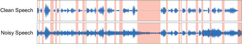
In this paper, we introduce a deep network for speech denoising that tightly integrates silent intervals, and thereby overcomes many of the limitations of classical approaches. Our goal is not just to identify a single silent interval, but to find as many as possible silent intervals over time. Indeed, silent intervals in speech appear in abundance: psycholinguistic studies have shown that there is almost always a pause after each sentence and even each word in speech [78, 21]. Each pause, however short, provides a silent interval revealing noise characteristics local in time. All together, these silent intervals assemble a time-varying picture of background noise, allowing the neural network to better denoise speech signals, even in presence of nonstationary noise (see Fig. 1).
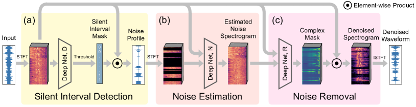
In short, to interleave neural networks with established denoising pipelines, we propose a network structure consisting of three major components (see Fig. 2): i) one dedicated to silent interval detection, ii) another that aims to estimate the full noise from those revealed in silent intervals, akin to an inpainting process in computer vision [38], and iii) yet another for cleaning up the input signal.
Summary of results. Our neural-network-based denoising model accepts a single channel of audio signal and outputs the cleaned-up signal. Unlike some of the recent denoising methods that take as input audiovisual signals (i.e., both audio and video footage), our method can be applied in a wider range of scenarios (e.g., in cellular communication). We conducted extensive experiments, including ablation studies to show the efficacy of our network components and comparisons to several state-of-the-art denoising methods. We also evaluate our method under various signal-to-noise ratios—even under strong noise levels that are not tested against in previous methods. We show that, under a variety of denoising metrics, our method consistently outperforms those methods, including those that accept only audio input (like ours) and those that denoise based on audiovisual input.
The pivotal role of silent intervals for speech denoising is further confirmed by a few key results. Even without supervising on silent interval detection, the ability to detect silent intervals naturally emerges in our network. Moreover, while our model is trained on English speech only, with no additional training it can be readily used to denoise speech in other languages (such as Chinese, Japanese, and Korean). Please refer to the supplementary materials for listening to our denoising results.
2 Related Work
Speech denoising.
Speech denoising [53] is a fundamental problem studied over several decades. Spectral subtraction [7, 98, 6, 72, 79] estimates the clean signal spectrum by subtracting an estimate of the noise spectrum from the noisy speech spectrum. This classic method was followed by spectrogram factorization methods [84]. Wiener filtering [80, 40] derives the enhanced signal by optimizing the mean-square error. Other methods exploit pauses in speech, forming segments of low acoustic energy where noise statistics can be more accurately measured [13, 57, 86, 15, 75, 10, 11]. Statistical model-based methods [14, 34] and subspace algorithms [12, 16] are also studied.
Applying neural networks to audio denoising dates back to the 80s [88, 69]. With increased computing power, deep neural networks are often used [104, 106, 105, 47]. Long short-term memory networks (LSTMs) [35] are able to preserve temporal context information of the audio signal [52], leading to strong results [56, 90, 100]. Leveraging generative adversarial networks (GANs) [33], methods such as [70, 71] have adopted GANs into the audio field and have also achieved strong performance.
Audio signal processing methods operate on either the raw waveform or the spectrogram by Short-time Fourier Transform (STFT). Some work directly on waveform [23, 68, 59, 55], and others use Wavenet [91] for speech denoising [74, 76, 30]. Many other methods such as [54, 94, 61, 99, 46, 107, 9] work on audio signal’s spectrogram, which contains both magnitude and phase information. There are works discussing how to use the spectrogram to its best potential [93, 67], while one of the disadvantages is that the inverse STFT needs to be applied. Meanwhile, there also exist works [51, 29, 28, 95, 19, 101, 60] investigating how to overcome artifacts from time aliasing.
Speech denoising has also been studied in conjunction with computer vision due to the relations between speech and facial features [8]. Methods such as [31, 26, 3, 36, 32] utilize different network structures to enhance the audio signal to the best of their ability. Adeel et al. [1] even utilize lip-reading to filter out the background noise of a speech.
Deep learning for other audio processing tasks.
Deep learning is widely used for lip reading, speech recognition, speech separation, and many audio processing or audio-related tasks, with the help of computer vision [64, 66, 5, 4]. Methods such as [50, 17, 65] are able to reconstruct speech from pure facial features. Methods such as [2, 63] take advantage of facial features to improve speech recognition accuracy. Speech separation is one of the areas where computer vision is best leveraged. Methods such as [25, 64, 18, 109] have achieved impressive results, making the previously impossible speech separation from a single audio signal possible. Recently, Zhang et al. [108] proposed a new operation called Harmonic Convolution to help networks distill audio priors, which is shown to even further improve the quality of speech separation.
3 Learning Speech Denoising
We present a neural network that harnesses the time distribution of silent intervals for speech denoising. The input to our model is a spectrogram of noisy speech [103, 20, 83], which can be viewed as a 2D image of size with two channels, where represents the time length of the signal and is the number of frequency bins. The two channels store the real and imaginary parts of STFT, respectively. After learning, the model will produce another spectrogram of the same size as the noise suppressed.
We first train our proposed network structure in an end-to-end fashion, with only denoising supervision (Sec. 3.2); and it already outperforms the state-of-the-art methods that we compare against. Furthermore, we incorporate the supervision on silent interval detection (Sec. 3.3) and obtain even better denoising results (see Sec. 4).
3.1 Network structure
Classic denoising algorithms work in three general stages: silent interval specification, noise feature estimation, and noise removal. We propose to interweave learning throughout this process: we rethink each stage with the help of a neural network, forming a new speech denoising model. Since we can chain these networks together and estimate gradients, we can efficiently train the model with large-scale audio data. Figure 2 illustrates this model, which we describe below.
Silent interval detection.
The first component is dedicated to detecting silent intervals in the input signal. The input to this component is the spectrogram of the input (noisy) signal . The spectrogram is first encoded by a 2D convolutional encoder into a 2D feature map, which is in turn processed by a bidirectional LSTM [35, 81] followed by two fully-connected (FC) layers (see network details in Appendix A). The bidirectional LSTM is suitable for processing time-series features resulting from the spectrogram [58, 41, 73, 18], and the FC layers are applied to the features of each time sample to accommodate variable length input. The output from this network component is a vector . Each element of is a scalar in [0,1] (after applying the sigmoid function), indicating a confidence score of a small time segment being silent. We choose each time segment to have second, small enough to capture short speech pauses and large enough to allow robust prediction.
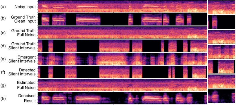
The output vector is then expanded to a longer mask, which we denote as . Each element of this mask indicates the confidence of classifying each sample of the input signal as pure noise (see Fig. 3-e). With this mask, the noise profile exposed by silent intervals are estimated by an element-wise product, namely .
Noise estimation.
The signal resulted from silent interval detection is noise profile exposed only through a series of time windows (see Fig. 3-e)—but not a complete picture of the noise. However, since the input signal is a superposition of clean speech signal and noise, having a complete noise profile would ease the denoising process, especially in presence of nonstationary noise. Therefore, we also estimate the entire noise profile over time, which we do with a neural network.
Inputs to this component include both the noisy audio signal and the incomplete noise profile . Both are converted by STFT into spectrograms, denoted as and , respectively. We view the spectrograms as 2D images. And because the neighboring time-frequency pixels in a spectrogram are often correlated, our goal here is conceptually akin to the image inpainting task in computer vision [38]. To this end, we encode and by two separate 2D convolutional encoders into two feature maps. The feature maps are then concatenated in a channel-wise manner and further decoded by a convolutional decoder to estimate the full noise spectrogram, which we denote as . A result of this step is illustrated in Fig. 3-f.
Noise removal.
Lastly, we clean up the noise from the input signal . We use a neural network that takes as input both the input audio spectrogram and the estimated full noise spectrogram . The two input spectrograms are processed individually by their own 2D convolutional encoders. The two encoded feature maps are then concatenated together before passing to a bidirectional LSTM followed by three fully connected layers (see details in Appendix A). Like other audio enhancement models [18, 92, 96], the output of this component is a vector with two channels which form the real and imaginary parts of a complex ratio mask in frequency-time domain. In other words, the mask has the same (temporal and frequency) dimensions as .
In the final step, we compute the denoised spectrogram through element-wise multiplication of the input audio spectrogram and the mask (i.e., ). Finally, the cleaned-up audio signal is obtained by applying the inverse STFT to (see Fig. 3-g).
3.2 Loss functions and training
Since a subgradient exists at every step, we are able to train our network in an end-to-end fashion with stochastic gradient descent. We optimize the following loss function:
| (1) |
where the notations , , , and are defined in Sec. 3.1; and denote the spectrograms of the ground-truth foreground signal and background noise, respectively. The first term penalizes the discrepancy between estimated noise and the ground-truth noise, while the second term accounts for the estimation of foreground signal. These two terms are balanced by the scalar ( in our experiments).
Natural emergence of silent intervals.
While producing plausible denoising results (see Sec. 4.4), the end-to-end training process has no supervision on silent interval detection: the loss function (1) only accounts for the recoveries of noise and clean speech signal. But somewhat surprisingly, the ability of detecting silent intervals automatically emerges as the output of the first network component (see Fig. 3-d as an example, which visualizes ). In other words, the network automatically learns to detect silent intervals for speech denoising without this supervision.
3.3 Silent interval supervision
As the model is learning to detect silent intervals on its own, we are able to directly supervise silent interval detection to further improve the denoising quality. Our first attempt was to add a term in (1) that penalizes the discrepancy between detected silent intervals and their ground truth. But our experiments show that this is not effective (see Sec. 4.4). Instead, we train our network in two sequential steps.
First, we train the silent interval detection component through the following loss function:
| (2) |
where is the binary cross entropy loss, is the mask resulted from silent interval detection component, and is the ground-truth label of each signal sample being silent or not—the way of constructing and the training dataset will be described in Sec. 4.1.
Next, we train the noise estimation and removal components through the loss function (1). This step starts by neglecting the silent detection component. In the loss function (1), instead of using , the noise spectrogram exposed by the estimated silent intervals, we use the noise spectrogram exposed by the ground-truth silent intervals (i.e., the STFT of ). After training using such a loss function, we fine-tune the network components by incorporating the already trained silent interval detection component. With the silent interval detection component fixed, this fine-tuning step optimizes the original loss function (1) and thereby updates the weights of the noise estimation and removal components.
4 Experiments
This section presents the major evaluations of our method, comparisons to several baselines and prior works, and ablation studies. We also refer the reader to the supplementary materials (including a supplemental document and audio effects organized on an off-line webpage) for the full description of our network structure, implementation details, additional evaluations, as well as audio examples.
4.1 Experiment setup
Dataset construction.
To construct training and testing data, we leverage publicly available audio datasets. We obtain clean speech signals using AVSPEECH [18], from which we randomly choose 2448 videos ( hours of total length) and extract their speech audio channels. Among them, we use 2214 videos for training and 234 videos for testing, so the training and testing speeches are fully separate. All these speech videos are in English, selected on purpose: as we show in supplementary materials, our model trained on this dataset can readily denoise speeches in other languages.
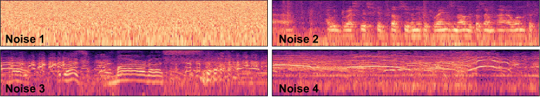
We use two datasets, DEMAND [89] and Google’s AudioSet [27], as background noise. Both consist of environmental noise, transportation noise, music, and many other types of noises. DEMAND has been used in previous denoising works (e.g., [70, 30, 90]). Yet AudioSet is much larger and more diverse than DEMAND, thus more challenging when used as noise. Figure 4 shows some noise examples. Our evaluations are conducted on both datasets, separately.
Due to the linearity of acoustic wave propagation, we can superimpose clean speech signals with noise to synthesize noisy input signals (similar to previous works [70, 30, 90]). When synthesizing a noisy input signal, we randomly choose a signal-to-noise ratio (SNR) from seven discrete values: -10dB, -7dB, -3dB, 0dB, 3dB, 7dB, and 10dB; and by mixing the foreground speech with properly scaled noise, we produce a noisy signal with the chosen SNR. For example, a -10dB SNR means that the power of noise is ten times the speech (see Fig. S1 in appendix). The SNR range in our evaluations (i.e., [-10dB, 10dB]) is significantly larger than those tested in previous works.
To supervise our silent interval detection (recall Sec. 3.3), we need ground-truth labels of silent intervals. To this end, we divide each clean speech signal into time segments, each of which lasts seconds. We label a time segment as silent when the total acoustic energy in that segment is below a threshold. Since the speech is clean, this automatic labeling process is robust.
Remarks on creating our own datasets. Unlike many previous models, which are trained using existing datasets such as Valentini’s VoiceBank-DEMAND [90], we choose to create our own datasets because of two reasons. First, Valentini’s dataset has a noise SNR level in [0dB, 15dB], much narrower than what we encounter in real-world recordings. Secondly, although Valentini’s dataset provides several kinds of environmental noise, it lacks the richness of other types of structured noise such as music, making it less ideal for denoising real-world recordings (see discussion in Sec. 4.6).
Method comparison.
We compare our method with several existing methods that are also designed for speech denoising, including both the classic approaches and recently proposed learning-based methods. We refer to these methods as follows: i) Ours, our model trained with silent interval supervision (recall Sec. 3.3); ii) Baseline-thres, a baseline method that uses acoustic energy threshold to label silent intervals (the same as our automatic labeling approach in Sec. 4.1 but applied on noisy input signals), and then uses our trained noise estimation and removal networks for speech denoising. iii) Ours-GTSI, another reference method that uses our trained noise estimation and removal networks, but hypothetically uses the ground-truth silent intervals; iv) Spectral Gating, the classic speech denoising algorithm based on spectral subtraction [79]; v) Adobe Audition [39], one of the most widely used professional audio processing software, and we use its machine-learning-based noise reduction feature, provided in the latest Adobe Audition CC 2020, with default parameters to batch process all our test data; vi) SEGAN [70], one of the state-of-the-art audio-only speech enhancement methods based on generative adversarial networks. vii) DFL [30], a recently proposed speech denoising method based on a loss function over deep network features; 111This recent method is designed for high-noise-level input, trained in an end-to-end fashion, and as their paper states, is “particularly pronounced for the hardest data with the most intrusive background noise”. viii) VSE [26], a learning-based method that takes both video and audio as input, and leverages both audio signal and mouth motions (from video footage) for speech denoising. We could not compare with another audiovisual method [18] because no source code or executable is made publicly available.
For fair comparisons, we train all the methods (except Spectral Gating which is not learning-based and Adobe Audition which is commercially shipped as a black box) using the same datasets. For SEGAN, DFL, and VSE, we use their source codes published by the authors. The audiovisual denoising method VSE also requires video footage, which is available in AVSPEECH.
4.2 Evaluation on speech denoising
Metrics.
Due to the perceptual nature of audio processing tasks, there is no widely accepted single metric for quantitative evaluation and comparisons. We therefore evaluate our method under six different metrics, all of which have been frequently used for evaluating audio processing quality. Namely, these metrics are: i) Perceptual Evaluation of Speech Quality (PESQ) [77], ii) Segmental Signal-to-Noise Ratio (SSNR) [82], iii) Short-Time Objective Intelligibility (STOI) [87], iv) Mean opinion score (MOS) predictor of signal distortion (CSIG) [37], v) MOS predictor of background-noise intrusiveness (CBAK) [37], and vi) MOS predictor of overall signal quality (COVL) [37].
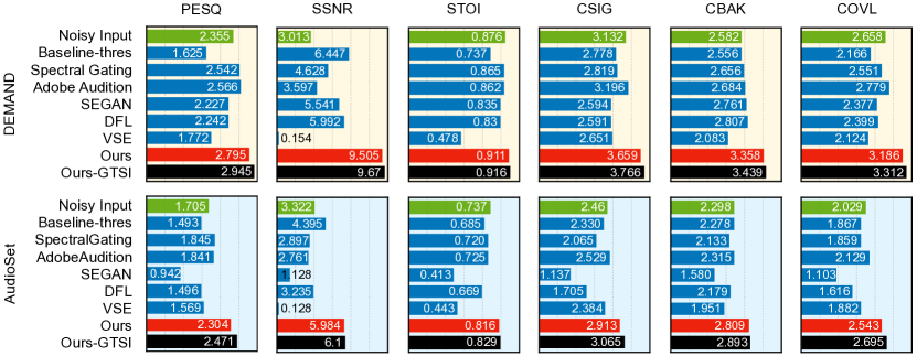
Results.
We train two separate models using DEMAND and AudioSet noise datasets respectively, and compare them with other models trained with the same datasets. We evaluate the average metric values and report them in Fig. 5. Under all metrics, our method consistently outperforms others.
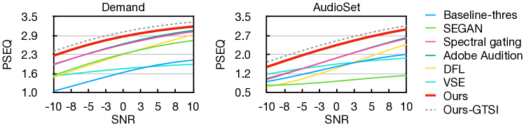
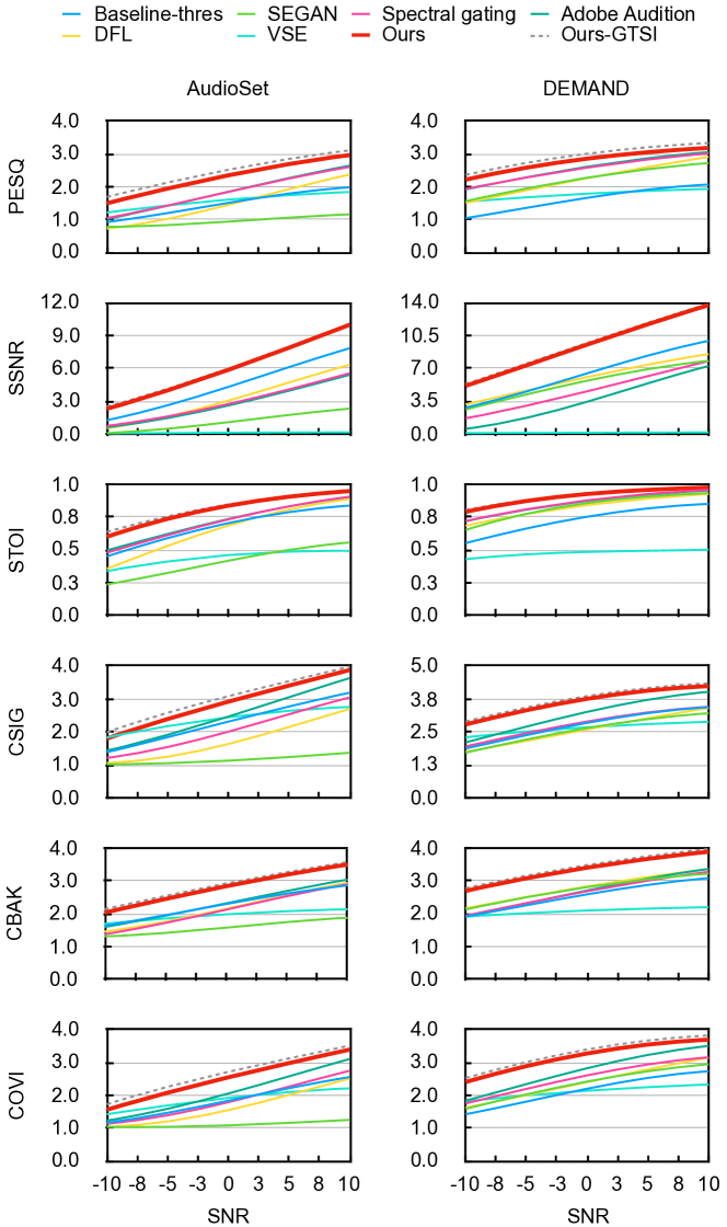
We breakdown the performance of each method with respect to SNR levels from -10dB to 10dB on both noise datasets. The results are reported in Fig. 6 for PESQ (see Fig. S2 in the appendix for all metrics). In the previous works that we compare to, no results under those low SNR levels (at dBs) are reported. Nevertheless, across all input SNR levels, our method performs the best, showing that our approach is fairly robust to both light and extreme noise.
From Fig. 6, it is worth noting that Ours-GTSI method performs even better. Recall that this is our model but provided with ground-truth silent intervals. While not practical (due to the need of ground-truth silent intervals), Ours-GTSI confirms the importance of silent intervals for denoising: a high-quality silent interval detection helps to improve speech denoising quality.
4.3 Evaluation on silent interval detection
Due to the importance of silent intervals for speech denoising, we also evaluate the quality of our silent interval detection, in comparison to two alternatives, the baseline Baseline-thres and a Voice Activity Detector (VAD) [22]. The former is described above, while the latter classifies each time window of an audio signal as having human voice or not [48, 49]. We use an off-the-shelf VAD [102], which is developed by Google’s WebRTC project and reported as one of the best available. Typically, VAD is designed to work with low-noise signals. Its inclusion here here is merely to provide an alternative approach that can detect silent intervals in more ideal situations.
We evaluate these methods using four standard statistic metrics: the precision, recall, F1 score, and accuracy. We follow the standard definitions of these metrics, which are summarized in Appendix C.1. These metrics are based on the definition of positive/negative conditions. Here, the positive condition indicates a time segment being labeled as a silent segment, and the negative condition indicates a non-silent label. Thus, the higher the metric values are, the better the detection approach.
| Noise Dataset | Method | Precision | Recall | F1 | Accuracy |
|---|---|---|---|---|---|
| DEMAND | Baseline-thres | 0.533 | 0.718 | 0.612 | 0.706 |
| VAD | 0.797 | 0.432 | 0.558 | 0.783 | |
| Ours | 0.876 | 0.866 | 0.869 | 0.918 | |
| Audioset | Baseline-thres | 0.536 | 0.731 | 0.618 | 0.708 |
| VAD | 0.736 | 0.227 | 0.338 | 0.728 | |
| Ours | 0.794 | 0.822 | 0.807 | 0.873 |
Table 1 shows that, under all metrics, our method is consistently better than the alternatives. Between VAD and Baseline-thres, VAD has higher precision and lower recall, meaning that VAD is overly conservative and Baseline-thres is overly aggressive when detecting silent intervals (see Fig. S3 in Appendix C.2). Our method reaches better balance and thus detects silent intervals more accurately.
4.4 Ablation studies
| Noise Dataset | Method | PESQ | SSNR | STOI | CSIG | CBAK | COVL |
|---|---|---|---|---|---|---|---|
| DEMAND | Ours w/o SID comp | 2.689 | 9.080 | 0.904 | 3.615 | 3.285 | 3.112 |
| Ours w/o NR comp | 2.476 | 0.234 | 0.747 | 3.015 | 2.410 | 2.637 | |
| Ours w/o SID loss | 2.794 | 6.478 | 0.903 | 3.466 | 3.147 | 3.079 | |
| Ours w/o NE loss | 2.601 | 9.070 | 0.896 | 3.531 | 3.237 | 3.027 | |
| Ours Joint loss | 2.774 | 6.042 | 0.895 | 3.453 | 3.121 | 3.068 | |
| Ours | 2.795 | 9.505 | 0.911 | 3.659 | 3.358 | 3.186 | |
| Audioset | Ours w/o SID comp | 2.190 | 5.574 | 0.802 | 2.851 | 2.719 | 2.454 |
| Ours w/o NR comp | 1.803 | 0.191 | 0.623 | 2.301 | 2.070 | 1.977 | |
| Ours w/o SID loss | 2.325 | 4.957 | 0.814 | 2.814 | 2.746 | 2.503 | |
| Ours w/o NE loss | 2.061 | 5.690 | 0.789 | 2.766 | 2.671 | 2.362 | |
| Ours Joint loss | 2.305 | 4.612 | 0.807 | 2.774 | 2.721 | 2.474 | |
| Ours | 2.304 | 5.984 | 0.816 | 2.913 | 2.809 | 2.543 |
In addition, we perform a series of ablation studies to understand the efficacy of individual network components and loss terms (see Appendix D.1 for more details). In Table 2, “Ours w/o SID loss” refers to the training method presented in Sec. 3.2 (i.e., without silent interval supervision). “Ours Joint loss” refers to the end-to-end training approach that optimizes the loss function (1) with the additional term (2). And “Ours w/o NE loss” uses our two-step training (in Sec. 3.3) but without the loss term on noise estimation—that is, without the first term in (1). In comparison to these alternative training approaches, our two-step training with silent interval supervision (referred to as “Ours”) performs the best. We also note that “Ours w/o SID loss”—i.e., without supervision on silent interval detection—already outperforms the methods we compared to in Fig. 5, and “Ours” further improves the denoising quality. This shows the efficacy of our proposed training approach.
We also experimented with two variants of our network structure. The first one, referred to as “Ours w/o SID comp”, turns off silent interval detection: the silent interval detection component always outputs a vector with all zeros. The second, referred as “Ours w/o NR comp”, uses a simple spectral subtraction to replace our noise removal component. Table 2 shows that, under all the tested metrics, both variants perform worse than our method, suggesting our proposed network structure is effective.
Furthermore, we studied to what extent the accuracy of silent interval detection affects the speech denoising quality. We show that as the silent interval detection becomes less accurate, the denoising quality degrades. Presented in details in Appendix D.2, these experiments reinforce our intuition that silent intervals are instructive for speech denoising tasks.
4.5 Comparison with state-of-the-art benchmark
Many state-of-the-art denoising methods, including MMSE-GAN [85], Metric-GAN [24], SDR-PESQ [43], T-GSA [44], Self-adaptation DNN [45], and RDL-Net [62], are all evaluated on Valentini’s VoiceBank-DEMAND [90]. We therefore compare ours with those methods on the same dataset. We note that DEMAND consists of audios with SNR in [0dB, 15dB]. Its SNR range is much narrower than what our method (and our training datasets) aims for (e.g., input signals with -10dB SNR). Nevertheless, trained and tested under the same setting, our method is highly competitive to the best of those methods under every metric, as shown in Table 3. The metric scores therein for other methods are numbers reported in their original papers.
| Method | PESQ | CSIG | CBAK | COVL | STOI |
|---|---|---|---|---|---|
| Noisy Input | 1.97 | 3.35 | 2.44 | 2.63 | 0.91 |
| WaveNet [91] | – | 3.62 | 3.24 | 2.98 | – |
| SEGAN [70] | 2.16 | 3.48 | 2.94 | 2.80 | 0.93 |
| DFL [30] | 2.51 | 3.79 | 3.27 | 3.14 | – |
| MMSE-GAN [85] | 2.53 | 3.80 | 3.12 | 3.14 | 0.93 |
| MetricGAN [24] | 2.86 | 3.99 | 3.18 | 3.42 | – |
| SDR-PESQ [43] | 3.01 | 4.09 | 3.54 | 3.55 | – |
| T-GSA [44] | 3.06 | 4.18 | 3.59 | 3.62 | – |
| Self-adapt. DNN [45] | 2.99 | 4.15 | 3.42 | 3.57 | – |
| RDL-Net [62] | 3.02 | 4.38 | 3.43 | 3.72 | 0.94 |
| Ours | 3.16 | 3.96 | 3.54 | 3.53 | 0.98 |
4.6 Tests on real-world data
We also test our method against real-world data. Quantitative evaluation on real-world data, however, is not easy because the evaluation of nearly all metrics requires the corresponding ground-truth clean signal, which is not available in real-world scenario. Instead, we collected a good number of real-world audios, either by recording in daily environments or by downloading online (e.g., from YouTube). These real-world audios cover diverse scenarios: in a driving car, a café, a park, on the street, in multiple languages (Chinese, Japanese, Korean, German, French, etc.), with different genders and accents, and even with singing songs. None of these recordings is cherry picked. We refer the reader to our project website for the denoising results of all the collected real-world recordings, and for the comparison of our method with other state-of-the-art methods under real-world settings.
Furthermore, we use real-world data to test our model trained with different datasets, including our own dataset (recall Sec. 4.1) and the existing DEMAND [90]. We show that the network model trained by our own dataset leads to much better noise reduction (see details in Appendix E.2). This suggests that our dataset allows the denoising model to better generalize to many real-world scenarios.
5 Conclusion
Speech denoising has been a long-standing challenge. We present a new network structure that leverages the abundance of silent intervals in speech. Even without silent interval supervision, our network is able to denoise speech signals plausibly, and meanwhile, the ability to detect silent intervals automatically emerges. We reinforce this ability. Our explicit supervision on silent intervals enables the network to detect them more accurately, thereby further improving the performance of speech denoising. As a result, under a variety of denoising metrics, our method consistently outperforms several state-of-the-art audio denoising models.
Acknowledgments.
This work was supported in part by the National Science Foundation (1717178, 1816041, 1910839, 1925157) and SoftBank Group.
Broader Impact
High-quality speech denoising is desired in a myriad of applications: human-robot interaction, cellular communications, hearing aids, teleconferencing, music recording, filmmaking, news reporting, and surveillance systems to name a few. Therefore, we expect our proposed denoising method—be it a system used in practice or a foundation for future technology—to find impact in these applications.
In our experiments, we train our model using English speech only, to demonstrate its generalization property—the ability of denoising spoken languages beyond English. Our demonstration of denoising Japanese, Chinese, and Korean speeches is intentional: they are linguistically and phonologically distant from English (in contrast to other English “siblings” such as German and Dutch). Still, our model may bias in favour of spoken languages and cultures that are closer to English or that have frequent pauses to reveal silent intervals. Deeper understanding of this potential bias requires future studies in tandem with linguistic and sociocultural insights.
Lastly, it is natural to extend our model for denoising audio signals in general or even signals beyond audio (such as Gravitational wave denoising [97]). If successful, our model can bring in even broader impacts. Pursuing this extension, however, requires a judicious definition of “silent intervals”. After all, the notion of “noise” in a general context of signal processing depends on specific applications: noise in one application may be another’s signals. To train a neural network that exploits a general notion of silent intervals, prudence must be taken to avoid biasing toward certain types of noise.
References
- Adeel et al. [2019] A. Adeel, M. Gogate, A. Hussain, and W. M. Whitmer. Lip-reading driven deep learning approach for speech enhancement. IEEE Transactions on Emerging Topics in Computational Intelligence, page 1–10, 2019. ISSN 2471-285x. doi: 10.1109/tetci.2019.2917039. URL http://dx.doi.org/10.1109/tetci.2019.2917039.
- Afouras et al. [2018] T. Afouras, J. S. Chung, A. Senior, O. Vinyals, and A. Zisserman. Deep audio-visual speech recognition. IEEE Transactions on Pattern Analysis and Machine Intelligence, pages 1–1, 2018.
- Afouras et al. [2018] T. Afouras, J. S. Chung, and A. Zisserman. The conversation: Deep audio-visual speech enhancement. In Proc. Interspeech 2018, pages 3244–3248, 2018. doi: 10.21437/Interspeech.2018-1400. URL http://dx.doi.org/10.21437/Interspeech.2018-1400.
- Arandjelovic and Zisserman [2018] R. Arandjelovic and A. Zisserman. Objects that sound. In Proceedings of the European Conference on Computer Vision (ECCV), pages 435–451, 2018.
- Aytar et al. [2016] Y. Aytar, C. Vondrick, and A. Torralba. Soundnet: Learning sound representations from unlabeled video. In Advances in neural information processing systems, pages 892–900, 2016.
- Berouti et al. [1979] M. Berouti, R. Schwartz, and J. Makhoul. Enhancement of speech corrupted by acoustic noise. In ICASSP ’79. IEEE International Conference on Acoustics, Speech, and Signal Processing, volume 4, pages 208–211, 1979.
- Boll [1979] S. Boll. Suppression of acoustic noise in speech using spectral subtraction. IEEE Transactions on Acoustics, Speech, and Signal Processing, 27(2):113–120, 1979.
- Busso and Narayanan [2007] C. Busso and S. S. Narayanan. Interrelation between speech and facial gestures in emotional utterances: A single subject study. IEEE Transactions on Audio, Speech, and Language Processing, 15(8):2331–2347, 2007.
- Chen and Wang [2017] J. Chen and D. Wang. Long short-term memory for speaker generalization in supervised speech separation. Acoustical Society of America Journal, 141(6):4705–4714, June 2017. doi: 10.1121/1.4986931.
- Cohen [2003] I. Cohen. Noise spectrum estimation in adverse environments: improved minima controlled recursive averaging. IEEE Transactions on Speech and Audio Processing, 11(5):466–475, 2003.
- Cohen and Berdugo [2002] I. Cohen and B. Berdugo. Noise estimation by minima controlled recursive averaging for robust speech enhancement. IEEE Signal Processing Letters, 9(1):12–15, 2002.
- Dendrinos et al. [1991] M. Dendrinos, S. Bakamidis, and G. Carayannis. Speech enhancement from noise: A regenerative approach. Speech Commun., 10(1):45–67, Feb. 1991. ISSN 0167-6393. doi: 10.1016/0167-6393(91)90027-q. URL https://doi.org/10.1016/0167-6393(91)90027-Q.
- Doblinger [1995] G. Doblinger. Computationally efficient speech enhancement by spectral minima tracking in subbands. In in Proc. Eurospeech, pages 1513–1516, 1995.
- Ephraim [1992] Y. Ephraim. Statistical-model-based speech enhancement systems. Proceedings of the IEEE, 80(10):1526–1555, 1992.
- Ephraim and Malah [1985] Y. Ephraim and D. Malah. Speech enhancement using a minimum mean-square error log-spectral amplitude estimator. IEEE Transactions on Acoustics, Speech, and Signal Processing, 33(2):443–445, 1985.
- Ephraim and Van Trees [1995] Y. Ephraim and H. L. Van Trees. A signal subspace approach for speech enhancement. IEEE Transactions on Speech and Audio Processing, 3(4):251–266, 1995.
- Ephrat et al. [2017] A. Ephrat, T. Halperin, and S. Peleg. Improved speech reconstruction from silent video. In 2017 IEEE International Conference on Computer Vision Workshops (ICCVW), pages 455–462, 2017.
- Ephrat et al. [2018] A. Ephrat, I. Mosseri, O. Lang, T. Dekel, K. Wilson, A. Hassidim, W. T. Freeman, and M. Rubinstein. Looking to listen at the cocktail party: A speaker-independent audio-visual model for speech separation. ACM Transactions on Graphics, 37(4):1–11, July 2018. ISSN 0730-0301. doi: 10.1145/3197517.3201357. URL http://dx.doi.org/10.1145/3197517.3201357.
- Erdogan et al. [2015] H. Erdogan, J. R. Hershey, S. Watanabe, and J. Le Roux. Phase-sensitive and recognition-boosted speech separation using deep recurrent neural networks. In 2015 IEEE International Conference on Acoustics, Speech and Signal Processing (ICASSP), pages 708–712, 2015.
- Flanagan [1972] J. L. Flanagan. Speech Analysis Synthesis and Perception. Springer-Verlag, 2nd edition, 1972. ISBN 9783662015629.
- Fors [2015] K. L. Fors. Production and perception of pauses in speech. PhD thesis, Department of Philosophy, Linguistics, and Theory of Science, University of Gothenburg, 2015.
- Freeman et al. [1989] D. K. Freeman, G. Cosier, C. B. Southcott, and I. Boyd. The voice activity detector for the pan-european digital cellular mobile telephone service. In International Conference on Acoustics, Speech, and Signal Processing,, pages 369–372 vol.1, 1989.
- Fu et al. [2017] S.-W. Fu, Y. Tsao, X. Lu, and H. Kawai. Raw waveform-based speech enhancement by fully convolutional networks. 2017 Asia-Pacific Signal and Information Processing Association Annual Summit and Conference (APSIPA ASC), Dec. 2017. doi: 10.1109/apsipa.2017.8281993. URL http://dx.doi.org/10.1109/APSIPA.2017.8281993.
- Fu et al. [2019] S.-W. Fu, C.-F. Liao, Y. Tsao, and S.-D. Lin. Metricgan: Generative adversarial networks based black-box metric scores optimization for speech enhancement, 2019.
- Gabbay et al. [2017a] A. Gabbay, A. Ephrat, T. Halperin, and S. Peleg. Seeing through noise: Visually driven speaker separation and enhancement, 2017a.
- Gabbay et al. [2017b] A. Gabbay, A. Shamir, and S. Peleg. Visual speech enhancement, 2017b.
- Gemmeke et al. [2017] J. F. Gemmeke, D. P. W. Ellis, D. Freedman, A. Jansen, W. Lawrence, R. C. Moore, M. Plakal, and M. Ritter. Audio set: An ontology and human-labeled dataset for audio events. In Proc. IEEE ICASSP 2017, New Orleans, LA, 2017.
- Gerkmann et al. [2015] T. Gerkmann, M. Krawczyk-Becker, and J. Le Roux. Phase processing for single-channel speech enhancement: History and recent advances. IEEE Signal Processing Magazine, 32(2):55–66, 2015.
- Germain et al. [2016] F. G. Germain, G. J. Mysore, and T. Fujioka. Equalization matching of speech recordings in real-world environments. In 2016 IEEE International Conference on Acoustics, Speech and Signal Processing (ICASSP), pages 609–613, 2016.
- Germain et al. [2019] F. G. Germain, Q. Chen, and V. Koltun. Speech denoising with deep feature losses. In Proc. Interspeech 2019, pages 2723–2727, 2019. doi: 10.21437/Interspeech.2019-1924. URL http://dx.doi.org/10.21437/Interspeech.2019-1924.
- Girin et al. [2001] L. Girin, J.-L. Schwartz, and G. Feng. Audio-visual enhancement of speech in noise. The Journal of the Acoustical Society of America, 109(6):3007–3020, 2001. doi: 10.1121/1.1358887. URL https://doi.org/10.1121/1.1358887.
- Gogate et al. [2019] M. Gogate, A. Adeel, K. Dashtipour, P. Derleth, and A. Hussain. Av speech enhancement challenge using a real noisy corpus, 2019.
- Goodfellow et al. [2014] I. J. Goodfellow, J. Pouget-Abadie, M. Mirza, B. Xu, D. Warde-Farley, S. Ozair, A. Courville, and Y. Bengio. Generative adversarial nets. In Proceedings of the 27th International Conference on Neural Information Processing Systems - Volume 2, Nips’14, page 2672–2680, Cambridge, MA, USA, 2014. MIT Press.
- Hirsch and Ehrlicher [1995] H.-G. Hirsch and C. Ehrlicher. Noise estimation techniques for robust speech recognition. 1995 International Conference on Acoustics, Speech, and Signal Processing, 1:153–156 vol.1, 1995.
- Hochreiter and Schmidhuber [1997] S. Hochreiter and J. Schmidhuber. Long short-term memory. Neural computation, 9:1735–80, 12 1997. doi: 10.1162/neco.1997.9.8.1735.
- Hou et al. [2018] J.-C. Hou, S.-S. Wang, Y.-H. Lai, Y. Tsao, H.-W. Chang, and H.-m. Wang. Audio-visual speech enhancement using multimodal deep convolutional neural networks. IEEE Transactions on Emerging Topics in Computational Intelligence, 2, 03 2018. doi: 10.1109/tetci.2017.2784878.
- Hu and Loizou [2008] Y. Hu and P. Loizou. Evaluation of objective quality measures for speech enhancement. Audio, Speech, and Language Processing, IEEE Transactions on, 16:229–238, 02 2008. doi: 10.1109/tasl.2007.911054.
- Iizuka et al. [2017] S. Iizuka, E. Simo-Serra, and H. Ishikawa. Globally and locally consistent image completion. ACM Trans. Graph., 36(4), July 2017. ISSN 0730-0301. doi: 10.1145/3072959.3073659. URL https://doi.org/10.1145/3072959.3073659.
- Inc. [2020] A. Inc. Adobe audition, 2020. URL https://www.adobe.com/products/audition.html.
- Jae Lim and Oppenheim [1978] Jae Lim and A. Oppenheim. All-pole modeling of degraded speech. IEEE Transactions on Acoustics, Speech, and Signal Processing, 26(3):197–210, 1978.
- Kalchbrenner et al. [2018] N. Kalchbrenner, E. Elsen, K. Simonyan, S. Noury, N. Casagrande, E. Lockhart, F. Stimberg, A. van den Oord, S. Dieleman, and K. Kavukcuoglu. Efficient neural audio synthesis, 2018.
- Kell and McDermott [2019] A. J. E. Kell and J. H. McDermott. Invariance to background noise as a signature of non-primary auditory cortex. Nature Communications, 10(1):3958, Sept. 2019. ISSN 2041-1723. doi: 10.1038/s41467-019-11710-y. URL https://doi.org/10.1038/s41467-019-11710-y.
- Kim et al. [2019] J. Kim, M. El-Kharmy, and J. Lee. End-to-end multi-task denoising for joint sdr and pesq optimization, 2019.
- Kim et al. [2020] J. Kim, M. El-Khamy, and J. Lee. T-gsa: Transformer with gaussian-weighted self-attention for speech enhancement. In ICASSP 2020 - 2020 IEEE International Conference on Acoustics, Speech and Signal Processing (ICASSP), pages 6649–6653, 2020.
- Koizumi et al. [2020] Y. Koizumi, K. Yatabe, M. Delcroix, Y. Masuyama, and D. Takeuchi. Speech enhancement using self-adaptation and multi-head self-attention, 2020.
- Kumar and Florencio [2016] A. Kumar and D. Florencio. Speech enhancement in multiple-noise conditions using deep neural networks. Interspeech 2016, Sept. 2016. doi: 10.21437/interspeech.2016-88. URL http://dx.doi.org/10.21437/Interspeech.2016-88.
- Kumar and Florêncio [2016] A. Kumar and D. A. F. Florêncio. Speech enhancement in multiple-noise conditions using deep neural networks. In Interspeech, 2016.
- Le Bouquin Jeannes and Faucon [1994] R. Le Bouquin Jeannes and G. Faucon. Proposal of a voice activity detector for noise reduction. Electronics Letters, 30(12):930–932, 1994.
- Le Bouquin Jeannes and Faucon [1995] R. Le Bouquin Jeannes and G. Faucon. Study of a voice activity detector and its influence on a noise reduction system. Speech Communication, 16(3):245–254, 1995. ISSN 0167-6393. doi: https://doi.org/10.1016/0167-6393(94)00056-G. URL http://www.sciencedirect.com/science/article/pii/016763939400056G.
- Le Cornu and Milner [2017] T. Le Cornu and B. Milner. Generating intelligible audio speech from visual speech. IEEE/ACM Transactions on Audio, Speech, and Language Processing, 25(9):1751–1761, 2017.
- Le Roux and Vincent [2013] J. Le Roux and E. Vincent. Consistent wiener filtering for audio source separation. IEEE Signal Processing Letters, 20(3):217–220, 2013.
- Lipton et al. [2015] Z. C. Lipton, J. Berkowitz, and C. Elkan. A critical review of recurrent neural networks for sequence learning, 2015.
- Loizou [2013] P. C. Loizou. Speech Enhancement: Theory and Practice. CRC Press, Inc., Usa, 2nd edition, 2013. ISBN 1466504218.
- Lu et al. [2013] X. Lu, Y. Tsao, S. Matsuda, and C. Hori. Speech enhancement based on deep denoising autoencoder. In Interspeech, 2013.
- Luo and Mesgarani [2019] Y. Luo and N. Mesgarani. Conv-tasnet: Surpassing ideal time–frequency magnitude masking for speech separation. IEEE/ACM Trans. Audio, Speech and Lang. Proc., 27(8):1256–1266, Aug. 2019. ISSN 2329-9290. doi: 10.1109/taslp.2019.2915167. URL https://doi.org/10.1109/TASLP.2019.2915167.
- Maas et al. [2012] A. L. Maas, Q. V. Le, T. M. O’Neil, O. Vinyals, P. Nguyen, and A. Y. Ng. Recurrent neural networks for noise reduction in robust asr. In Interspeech, 2012.
- Martin [2001] R. Martin. Noise power spectral density estimation based on optimal smoothing and minimum statistics. IEEE Transactions on Speech and Audio Processing, 9(5):504–512, 2001.
- Mehri et al. [2016] S. Mehri, K. Kumar, I. Gulrajani, R. Kumar, S. Jain, J. Sotelo, A. Courville, and Y. Bengio. Samplernn: An unconditional end-to-end neural audio generation model, 2016.
- Michelashvili and Wolf [2019] M. Michelashvili and L. Wolf. Audio denoising with deep network priors, 2019.
- Moorer [2017] J. A. Moorer. A note on the implementation of audio processing by short-term fourier transform. In 2017 IEEE Workshop on Applications of Signal Processing to Audio and Acoustics (WASPAA), pages 156–159, 2017.
- Narayanan and Wang [2013] A. Narayanan and D. Wang. Ideal ratio mask estimation using deep neural networks for robust speech recognition. In 2013 IEEE International Conference on Acoustics, Speech and Signal Processing, pages 7092–7096, 2013.
- Nikzad et al. [2020] M. Nikzad, A. Nicolson, Y. Gao, J. Zhou, K. K. Paliwal, and F. Shang. Deep residual-dense lattice network for speech enhancement, 2020.
- Noda et al. [2015] K. Noda, Y. Yamaguchi, K. Nakadai, H. G. Okuno, and T. Ogata. Audio-visual speech recognition using deep learning. Applied Intelligence, 42(4):722–737, June 2015. ISSN 0924-669x. doi: 10.1007/s10489-014-0629-7. URL https://doi.org/10.1007/s10489-014-0629-7.
- Owens and Efros [2018] A. Owens and A. A. Efros. Audio-visual scene analysis with self-supervised multisensory features. Lecture Notes in Computer Science, page 639–658, 2018. ISSN 1611-3349. doi: 10.1007/978-3-030-01231-1\_39. URL http://dx.doi.org/10.1007/978-3-030-01231-1%5F39.
- Owens et al. [2016a] A. Owens, P. Isola, J. McDermott, A. Torralba, E. H. Adelson, and W. T. Freeman. Visually indicated sounds. 2016 IEEE Conference on Computer Vision and Pattern Recognition (CVPR), June 2016a. doi: 10.1109/cvpr.2016.264. URL http://dx.doi.org/10.1109/CVPR.2016.264.
- Owens et al. [2016b] A. Owens, J. Wu, J. H. McDermott, W. T. Freeman, and A. Torralba. Ambient sound provides supervision for visual learning. In European conference on computer vision, pages 801–816. Springer, 2016b.
- Paliwal et al. [2011] K. Paliwal, K. Wójcicki, and B. Shannon. The importance of phase in speech enhancement. Speech Commun., 53(4):465–494, Apr. 2011. ISSN 0167-6393. doi: 10.1016/j.specom.2010.12.003. URL https://doi.org/10.1016/j.specom.2010.12.003.
- Pandey and Wang [2018] A. Pandey and D. Wang. A new framework for supervised speech enhancement in the time domain. In Proc. Interspeech 2018, pages 1136–1140, 2018. doi: 10.21437/Interspeech.2018-1223. URL http://dx.doi.org/10.21437/Interspeech.2018-1223.
- Parveen and Green [2004] S. Parveen and P. Green. Speech enhancement with missing data techniques using recurrent neural networks. In 2004 IEEE International Conference on Acoustics, Speech, and Signal Processing, volume 1, pages I–733, 2004.
- Pascual et al. [2017] S. Pascual, A. Bonafonte, and J. Serrà. Segan: Speech enhancement generative adversarial network. In Proc. Interspeech 2017, pages 3642–3646, 2017. doi: 10.21437/Interspeech.2017-1428. URL http://dx.doi.org/10.21437/Interspeech.2017-1428.
- Pascual et al. [2019] S. Pascual, J. Serrà, and A. Bonafonte. Towards generalized speech enhancement with generative adversarial networks. In Proc. Interspeech 2019, pages 1791–1795, 2019. doi: 10.21437/Interspeech.2019-2688. URL http://dx.doi.org/10.21437/Interspeech.2019-2688.
- ping Yang and Fu [2005] L. ping Yang and Q.-J. Fu. Spectral subtraction-based speech enhancement for cochlear implant patients in background noise. The Journal of the Acoustical Society of America, 117 3 Pt 1:1001–4, 2005.
- Purwins et al. [2019] H. Purwins, B. Li, T. Virtanen, J. Schluter, S.-Y. Chang, and T. Sainath. Deep learning for audio signal processing. IEEE Journal of Selected Topics in Signal Processing, 13(2):206–219, May 2019. ISSN 1941-0484. doi: 10.1109/jstsp.2019.2908700. URL http://dx.doi.org/10.1109/JSTSP.2019.2908700.
- Qian et al. [2017] K. Qian, Y. Zhang, S. Chang, X. Yang, D. Florêncio, and M. Hasegawa-Johnson. Speech enhancement using bayesian wavenet. In Proc. Interspeech 2017, pages 2013–2017, 2017. doi: 10.21437/Interspeech.2017-1672. URL http://dx.doi.org/10.21437/Interspeech.2017-1672.
- Rangachari et al. [2004] S. Rangachari, P. C. Loizou, and Yi Hu. A noise estimation algorithm with rapid adaptation for highly nonstationary environments. In 2004 IEEE International Conference on Acoustics, Speech, and Signal Processing, volume 1, pages I–305, 2004.
- Rethage et al. [2018] D. Rethage, J. Pons, and X. Serra. A wavenet for speech denoising. In 2018 IEEE International Conference on Acoustics, Speech and Signal Processing (ICASSP), pages 5069–5073, 2018.
- Rix et al. [2001] A. Rix, J. Beerends, M. Hollier, and A. Hekstra. Perceptual evaluation of speech quality (pesq): A new method for speech quality assessment of telephone networks and codecs. In 2001 IEEE International Conference on Acoustics, Speech, and Signal Processing. Proceedings (Cat. No.01CH37221), volume 2, pages 749–752 vol.2, 02 2001. ISBN 0-7803-7041-4. doi: 10.1109/icassp.2001.941023.
- Rochester [1973] S. R. Rochester. The significance of pauses in spontaneous speech. Journal of Psycholinguistic Research, 2(1):51–81, 1973.
- Sainburg [2019] T. Sainburg. Noise reduction in python using spectral gating. https://github.com/timsainb/noisereduce, 2019.
- Scalart and Filho [1996] P. Scalart and J. V. Filho. Speech enhancement based on a priori signal to noise estimation. In 1996 IEEE International Conference on Acoustics, Speech, and Signal Processing Conference Proceedings, volume 2, pages 629–632 vol. 2, 1996.
- Schuster and Paliwal [1997] M. Schuster and K. Paliwal. Bidirectional recurrent neural networks. Signal Processing, IEEE Transactions on, 45:2673–2681, 12 1997. doi: 10.1109/78.650093.
- Schuyler R. Quackenbush [1988] M. A. C. Schuyler R. Quackenbush, Thomas P. Barnwell. Objective Measures Of Speech Quality. Prentice Hall, Englewood Cliffs, NJ, 1988. ISBN 9780136290568.
- Sejdic et al. [2008] E. Sejdic, I. Djurovic, and L. Stankovic. Quantitative performance analysis of scalogram as instantaneous frequency estimator. IEEE Transactions on Signal Processing, 56(8):3837–3845, 2008.
- Smaragdis et al. [2014] P. Smaragdis, C. Févotte, G. J. Mysore, N. Mohammadiha, and M. Hoffman. Static and dynamic source separation using nonnegative factorizations: A unified view. IEEE Signal Processing Magazine, 31(3):66–75, 2014.
- Soni et al. [2018] M. H. Soni, N. Shah, and H. A. Patil. Time-frequency masking-based speech enhancement using generative adversarial network. In 2018 IEEE International Conference on Acoustics, Speech and Signal Processing (ICASSP), pages 5039–5043, 2018.
- Sørensen and Andersen [2005] K. V. Sørensen and S. V. Andersen. Speech enhancement with natural sounding residual noise based on connected time-frequency speech presence regions. EURASIP J. Adv. Signal Process, 2005:2954–2964, Jan. 2005. ISSN 1110-8657. doi: 10.1155/asp.2005.2954. URL https://doi.org/10.1155/ASP.2005.2954.
- Taal et al. [2010] C. Taal, R. Hendriks, R. Heusdens, and J. Jensen. A short-time objective intelligibility measure for time-frequency weighted noisy speech. In 2010 IEEE International Conference on Acoustics, Speech and Signal Processing, pages 4214–4217, 04 2010. doi: 10.1109/icassp.2010.5495701.
- Tamura and Waibel [1988] S. Tamura and A. Waibel. Noise reduction using connectionist models. In ICASSP-88., International Conference on Acoustics, Speech, and Signal Processing, pages 553–556 vol.1, 1988.
- Thiemann et al. [2013] J. Thiemann, N. Ito, and E. Vincent. The diverse environments multi-channel acoustic noise database (demand): A database of multichannel environmental noise recordings. In 21st International Congress on Acoustics, Montreal, Canada, June 2013. Acoustical Society of America. doi: 10.5281/zenodo.1227120. URL https://hal.inria.fr/hal-00796707. The dataset itself is archived on Zenodo, with DOI 10.5281/zenodo.1227120.
- Valentini-Botinhao et al. [2016] C. Valentini-Botinhao, X. Wang, S. Takaki, and J. Yamagishi. Investigating rnn-based speech enhancement methods for noise-robust text-to-speech. In 9th ISCA Speech Synthesis Workshop, pages 146–152, 2016. doi: 10.21437/ssw.2016-24. URL http://dx.doi.org/10.21437/SSW.2016-24.
- van den Oord et al. [2016] A. van den Oord, S. Dieleman, H. Zen, K. Simonyan, O. Vinyals, A. Graves, N. Kalchbrenner, A. W. Senior, and K. Kavukcuoglu. Wavenet: A generative model for raw audio. ArXiv, abs/1609.03499, 2016.
- Wang and Chen [2018] D. Wang and J. Chen. Supervised speech separation based on deep learning: An overview. IEEE/ACM Transactions on Audio, Speech, and Language Processing, 26(10):1702––1726, Oct. 2018. ISSN 2329-9304. doi: 10.1109/taslp.2018.2842159. URL http://dx.doi.org/10.1109/TASLP.2018.2842159.
- Wang and Jae Lim [1982] D. Wang and Jae Lim. The unimportance of phase in speech enhancement. IEEE Transactions on Acoustics, Speech, and Signal Processing, 30(4):679–681, 1982.
- Wang and Wang [2012] Y. Wang and D. Wang. Cocktail party processing via structured prediction. In Proceedings of the 25th International Conference on Neural Information Processing Systems - Volume 1, Nips’12, page 224–232, Red Hook, NY, USA, 2012. Curran Associates Inc.
- Wang and Wang [2015] Y. Wang and D. Wang. A deep neural network for time-domain signal reconstruction. In 2015 IEEE International Conference on Acoustics, Speech and Signal Processing (ICASSP), pages 4390–4394, 2015.
- Wang et al. [2014] Y. Wang, A. Narayanan, and D. Wang. On training targets for supervised speech separation. IEEE/ACM Transactions on Audio, Speech, and Language Processing, 22(12):1849–1858, 2014.
- Wei and Huerta [2020] W. Wei and E. Huerta. Gravitational wave denoising of binary black hole mergers with deep learning. Physics Letters B, 800:135081, 2020.
- Weiss et al. [1974] M. R. Weiss, E. Aschkenasy, and T. W. Parsons. Study and development of the intel technique for improving speech intelligibility. Technical report nsc-fr/4023, Nicolet Scientific Corporation, 1974.
- Weninger et al. [2014] F. Weninger, J. R. Hershey, J. Le Roux, and B. Schuller. Discriminatively trained recurrent neural networks for single-channel speech separation. In 2014 IEEE Global Conference on Signal and Information Processing (GlobalSIP), pages 577–581, 2014.
- Weninger et al. [2015] F. Weninger, H. Erdogan, S. Watanabe, E. Vincent, J. Roux, J. R. Hershey, and B. Schuller. Speech enhancement with lstm recurrent neural networks and its application to noise-robust asr. In Proceedings of the 12th International Conference on Latent Variable Analysis and Signal Separation - Volume 9237, Lva/ica 2015, page 91–99, Berlin, Heidelberg, 2015. Springer-Verlag. ISBN 9783319224817. doi: 10.1007/978-3-319-22482-4\_11. URL https://doi.org/10.1007/978-3-319-22482-4%5F11.
- Williamson and Wang [2017] D. S. Williamson and D. Wang. Time-frequency masking in the complex domain for speech dereverberation and denoising. IEEE/ACM Transactions on Audio, Speech, and Language Processing, 25(7):1492–1501, 2017.
- Wiseman [2019] J. Wiseman. py-webrtcvad. https://github.com/wiseman/py-webrtcvad, 2019.
- Wyse [2017] L. Wyse. Audio spectrogram representations for processing with convolutional neural networks, 2017.
- Xu et al. [2014] Y. Xu, J. Du, L. Dai, and C. Lee. An experimental study on speech enhancement based on deep neural networks. IEEE Signal Processing Letters, 21(1):65–68, 2014.
- Xu et al. [2015] Y. Xu, J. Du, L. Dai, and C. Lee. A regression approach to speech enhancement based on deep neural networks. IEEE/ACM Transactions on Audio, Speech, and Language Processing, 23(1):7–19, 2015.
- Xu et al. [2015] Y. Xu, J. Du, Z. Huang, L.-R. Dai, and C.-H. Lee. Multi-objective learning and mask-based post-processing for deep neural network based speech enhancement. In Interspeech, 2015.
- Zhang and Wang [2016] X. Zhang and D. Wang. A deep ensemble learning method for monaural speech separation. IEEE/ACM Transactions on Audio, Speech, and Language Processing, 24(5):967–977, 2016.
- Zhang et al. [2020] Z. Zhang, Y. Wang, C. Gan, J. Wu, J. B. Tenenbaum, A. Torralba, and W. T. Freeman. Deep audio priors emerge from harmonic convolutional networks. In International Conference on Learning Representations, 2020. URL https://openreview.net/forum?id=rygjHxrYDB.
- Zhao et al. [2018] H. Zhao, C. Gan, A. Rouditchenko, C. Vondrick, J. McDermott, and A. Torralba. The sound of pixels. In Proceedings of the European Conference on Computer Vision (ECCV), pages 570–586, 2018.
Supplementary Document
Listening to Sounds of Silence for Speech Denoising
Appendix A Network Structure and Training Details
We now present the details of our network structure and training configurations.
The silent interval detection component of our model is composed of 2D convolutional layers, a bidirectional LSTM, and two FC layers. The parameters of the convolutional layers are shown in Table S1. Each convolutional layer is followed by a batch normalization layer with a ReLU activation function. The hidden size of bidirectional LSTM is . The two FC layers, interleaved with a ReLU activation function, have hidden size of and , respectively.
| conv1 | conv2 | conv3 | conv4 | conv5 | conv6 | conv7 | conv8 | conv9 | conv10 | conv11 | conv12 | |
| Num Filters | 48 | 48 | 48 | 48 | 48 | 48 | 48 | 48 | 48 | 48 | 48 | 8 |
| Filter Size | (1,7) | (7,1) | (5,5) | (5,5) | (5,5) | (5,5) | (5,5) | (5,5) | (5,5) | (5,5) | (5,5) | (1,1) |
| Dilation | (1,1) | (1,1) | (1,1) | (2,1) | (4,1) | (8,1) | (16,1) | (32,1) | (1,1) | (2,2) | (4,4) | (1,1) |
| Stride | 1 | 1 | 1 | 1 | 1 | 1 | 1 | 1 | 1 | 1 | 1 | 1 |
The noise estimation component of our model is fully convolutional, consisting of two encoders and one decoder. The two encoders process the noisy signal and the incomplete noise profile, respectively; they have the same architecture (shown in Table S2) but different weights. The two feature maps resulted from the two encoders are concatenated in a channel-wise manner before feeding into the decoder. In Table S2, every layer, except the last one, is followed by a batch normalization layer together with a ReLU activation function. In addition, there is skip connections between the nd and -th layer and between the -th and -th layer.
| Encoder | Decoder | ||||||||||||||||
|---|---|---|---|---|---|---|---|---|---|---|---|---|---|---|---|---|---|
| ID | 1 | 2 | 3 | 4 | 5 | 6 | 7 | 8 | 9 | 10 | 11 | 12 | 13 | 14 | 15 | 16 | |
| Layer Type | C | C | C | C | C | C | C | C | C | C | C | TC | C | TC | C | C | |
| Num Filters | 64 | 128 | 128 | 256 | 256 | 256 | 256 | 256 | 256 | 256 | 256 | 128 | 128 | 64 | 64 | 2 | |
| Filter Size | 5 | 5 | 5 | 3 | 3 | 3 | 3 | 3 | 3 | 3 | 3 | 3 | 3 | 3 | 3 | 3 | |
| Dilation | 1 | 1 | 1 | 1 | 1 | 2 | 4 | 8 | 16 | 1 | 1 | 1 | 1 | 1 | 1 | 1 | |
| Stride | 1 | 2 | 1 | 2 | 1 | 1 | 1 | 1 | 1 | 1 | 1 | 2 | 1 | 2 | 1 | 1 | |
The noise removal component of our model is composed of two 2D convolutional encoders, a bidirectional LSTM, and three FC layers. The two convolutional encoders take as input the input audio spectrogram and the estimated full noise spectrogram , respectively. The first encoder has the network architecture listed in Table S3, and the second has the same architecture but with half of the number of filters at each convolutional layer. Moreover, the bidirectional LSTM has the hidden size of 200, and the three FC layers have the hidden size of 600, 600, and , respectively, where is the number of frequency bins in the spectrogram. In terms of the activation function, ReLU is used after each layer except the last layer, which uses sigmoid.
| C1 | C2 | C3 | C4 | C5 | C6 | C7 | C8 | C9 | C10 | C11 | C12 | C13 | C14 | C15 | |
| Num Filters | 96 | 96 | 96 | 96 | 96 | 96 | 96 | 96 | 96 | 96 | 96 | 96 | 96 | 96 | 8 |
| Filter Size | (1,7) | (7,1) | (5,5) | (5,5) | (5,5) | (5,5) | (5,5) | (5,5) | (5,5) | (5,5) | (5,5) | (5,5) | (5,5) | (5,5) | (1,1) |
| Dilation | (1,1) | (1,1) | (1,1) | (2,1) | (4,1) | (8,1) | (16,1) | (32,1) | (1,1) | (2,2) | (4,4) | (8,8) | (16,16) | (32,32) | (1,1) |
| Stride | 1 | 1 | 1 | 1 | 1 | 1 | 1 | 1 | 1 | 1 | 1 | 1 | 1 | 1 | 1 |
Training details.
We use PyTorch platform to implement our speech denoising model, which is then trained with the Adam optimizer. In our end-to-end training without silent interval supervision (referred to as “Ours w/o SID loss” in Sec. 4; also recall Sec. 3.2), we run the Adam optimizer for 50 epochs with a batch size of 20 and a learning rate of 0.001. When the silent interval supervision is incorporated (recall Sec. 3.3), we first train the silent interval detection component with the following setup: run the Adam optimizer for 100 epochs with a batch size of 15 and a learning rate of 0.001. Afterwards, we train the noise estimation and removal components using the same setup as the end-to-end training of “Ours w/o SID loss”.
Appendix B Data Processing Details
Our model is designed to take as input a mono-channel audio clip of an arbitrary length. However, when constructing the training dataset, we set each audio clip in the training dataset to have the same 2-second length, to enable batching at training time. To this end, we split each original audio clip from AVSPEECH, DEMAND, and AudioSet into 2-second long clips. All audio clips are then downsampled at 16kHz before converting into spectrograms using STFT. To perform STFT, the Fast Fourier Transform (FFT) size is set to 510, the Hann window size is set to 28ms, and the hop length is set to 11ms. As a result, each 2-second clip yields a (complex-valued) spectrogram with a resolution , where is the number of frequency bins, and 178 is the temporal resolution. At inference time, our model can still accept audio clips with arbitrary length.
Both our clean speech dataset and noise datasets are first split into training and test sets, so that no audio clips in training and testing are from the same original audio source—they are fully separate.
To supervise our silent interval detection, we label the clean audio signals in the following way. We first normalize each audio clip so that its magnitude is in the range [-1,1], that is, ensuring the largest waveform magnitude at -1 or 1. Then, the clean audio clip is divided into segments of length seconds. We label a time segment as a “silent” segment (i.e., label 0) if its average waveform energy in that segment is below 0.08. Otherwise, it is labeled as a “non-silent” segment (i.e., label 1).
Appendix C Evaluation on Silent Interval Detection
C.1 Metrics
We now provide the details of the metrics used for evaluating our silent interval detection (i.e., results in Table 1 of the main text). Detecting silent intervals is a binary classification task, one that classifies every time segment as being silent (i.e., a positive condition) or not (i.e., a negative condition). Recall that the confusion matrix in a binary classification task is as follows:
| Actual | |||
|---|---|---|---|
| Positive | Negative | ||
| Predicted | Positive | True Positive (TP) | False Positive (FP) |
| Negative | False Negative (FN) | True Negative (TN) | |
In our case, we have the following conditions:
-
•
A true positive (TP) sample is a correctly predicted silent segment.
-
•
A true negative (TN) sample is a correctly predicted non-silent segment.
-
•
A false positive (FP) sample is a non-silent segment predicted as silent.
-
•
A false negative (FN) sample is a silent segment predicted as non-silent.
The four metrics used in Table 1 follow the standard definitions in statistics, which we review here:
| (S1) |
where , , , and indicate the numbers of true positive, true negative, false positive, and false negative predictions among all tests. Intuitively, recall indicates the ability of correctly finding all true silent intervals, precision measures how much proportion of the labeled silent intervals are truly silent. F1 score takes both precision and recall into account, and produces their harmonic mean. And accuracy is the ratio of correct predictions among all predictions.
C.2 An Example of Silent Interval Detection
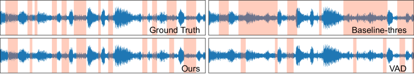
In Fig. S3, we present an example of silent interval detection results in comparison to two alternative methods. The two alternatives, described in Sec. 4.3, are referred to as Baseline-thres and VAD, respectively. Figure S3 echos the quantitative results in Table 1: VAD tends to be overly conservative, even in the presence of mild noise; and many silent intervals are ignored. On the other hand, Baseline-thres tends to be too aggressive; it produces many false intervals. In contrast, our silent interval detection maintains a better balance, and thus predicts more accurately.
Appendix D Ablation Studies and Analysis
D.1 Details of Ablation Studies
In Sec. 4.4 and Table 2, the ablation studies are set up in the following way.
- •
-
•
“Ours w/o SID loss” refers to our proposed network structure but optimized by the training method in Sec. 3.2 (i.e. an end-to-end training without silent interval supervision). This ablation study is to confirm that silent interval supervision indeed helps to improve the denoising quality.
-
•
“Ours Joint loss” refers to our proposed network structure optimized by the end-to-end training approach that optimizes the loss function (1) with the additional term (2). In this end-to-end training, silent interval detection is also supervised through the loss function. This ablation study is to confirm that our two-step training (Sec. 3.3) is more effective.
- •
-
•
“Ours w/o SID comp” turns off silent interval detection: the silent interval detection component always outputs a vector with all zeros. As a result, the input noise profile to the noise estimation component is made precisely the same as the original noisy signal. This ablation study is to examine the effect of silent intervals for speech denoising.
-
•
“Ours w/o NR comp” uses a simple spectral subtraction to replace our noise removal component; the other components remain unchanged. This ablation studey is to examine the efficacy of our noise removal component.
D.2 The Influence of Silent Interval Detection on Denoising Quality
A key insight of our neural-network-based denoising model is the leverage of silent interval distribution over time. The experiments above have confirmed the efficacy of our silent interval detection for better speech denoising. We now report additional experiments, aiming to gain some empirical understanding of how the quality of silent interval prediction would affect speech denoising quality.
| Shift | No Shift | 1/30 | 1/10 | 1/5 | 1/2 |
| PESQ | 2.471 | 1.932 | 1.317 | 1.169 | 1.094 |
| Shrink | No Shrink | 20% | 40% | 60% | 80% |
| PESQ | 2.471 | 2.361 | 2.333 | 2.283 | 2.249 |
First, starting with ground-truth silent intervals, we shift them on the time axis by , , , and seconds. As the shifted time amount increases, more time segments become incorrectly labeled: both the numbers of false positive labels (i.e., non-silent time segments labeled silent) and false negative labels (i.e., silent time segments are labeled non-silent) increase. After each shift, we feed the silent interval labels to our noise estimation and removal components and measure the denoising quality under the PESQ score.
In the second experiment, we again start with ground-truth silent intervals; but instead of shifting them, we shrink each silent interval toward its center by , , , and . As the silent intervals become more shrunken, fewer time segments are labeled as silent. In other words, only the number of false negative predictions increases. Similar to the previous experiment, after each shrink, we use the silent interval labels in our speech denoising pipeline, and meausure the PESQ score.
The results of both experiments are reported in Table S5. As we shrink the silent intervals, the denoising quality drops gently. In contrast, even a small amount of shift causes a clear drop of denoising quality. These results suggest that in comparison to false negative predictions, false positive predictions affect the denoising quality more negatively. On the one hand, reasonably conservative predictions may leave certain silent time segments undetected (i.e., introducing some false negative labels), but the detected silent intervals indeed reveal the noise profile. On the other hand, even a small amount of false positive predictions causes certain non-silent time segments to be treated as silent segments, and thus the observed noise profile through the detected silent intervals would be tainted by foreground signals.
Appendix E Evaluation of Model Performance
E.1 Generalization Across Datasets
To evaluate the generalization ability of our model, we performed three cross-dataset tests reported in Table S6. The experiments are set up in the following way.
-
•
“Test i”: We train our model on our own AVSPEECH+Audioset (AA) dataset but evaluate on Valentini’s VoiceBank-DEMAND (VD) testset. The result is shown in the first row of the “Test i” section in Table S6. In comparison, the second row shows the result of training on VD and testing on VD.
-
•
“Test ii”: We train our model on our own AA dataset but evaluate on our second AVSPEECH+DEMAND (AD) testset. The result is shown in the first row of the “Test ii” section in Table S6. In comparison, the second row shows the result of training on AD and testing on AD.
-
•
“Test iii”: We train our model on our own AD dataset but evaluate on AA testset. The result is shown in the first row of the “Test iii” section of the table. In comparison, the second row shows the result of training on AA and testing on AA.
The small degradation in each cross-dataset test demonstrates the great generalization ability of our method. We could not directly compare the generalization ability of our model with existing methods, as no previous work reported cross-dataset evaluation results.
| Test | Trainset | Testset | PESQ | CSIG | CBAK | COVL | STOI |
|---|---|---|---|---|---|---|---|
| Test i | AA | VD | 3.00 | 3.78 | 3.08 | 3.34 | 0.98 |
| VD | VD | 3.16 | 3.96 | 3.54 | 3.53 | 0.98 | |
| Test ii | AA | AD | 2.65 | 3.48 | 3.21 | 3.01 | 0.90 |
| AD | AD | 2.80 | 3.66 | 3.36 | 3.17 | 0.91 | |
| Test iii | AD | AA | 2.12 | 2.71 | 2.65 | 2.34 | 0.79 |
| AA | AA | 2.30 | 2.91 | 2.81 | 2.54 | 0.82 |
E.2 Generalization on Real-world Data
We conduct experiments to understand the extent to which the model trained with different datasets can generalize to real-world data. We train two versions of our model using our AVSPEECH+Audioset dataset and Valentini’s VoiceBank-DEMAND, respectively (denoted as “Model AA” and “Model VD”, respectively, in Table S7), and use them to denoise our collected real-world recordings. For the denoised real-world audios, we measure the noise level reduction in detected silent intervals. This measurement is doable, since it requires no knowledge of noise-free ground-truth audios. As shown in Table S7, in terms of noise reduction, the model trained with our own AA dataset outperforms the one trained with the public VoiceBank-DEMAND dataset by a significant amount for all tested real-world recordings. On average, it produces 22.3 dB noise reduction in comparison to 12.6 dB, suggesting that our dataset allows the denoising model to better generalize to many real-world scenarios.
| Real-world Recording | Model AA noise reduction (dB) | Model VD noise reduction (dB) |
|---|---|---|
| Song Excerpt 1 | 22.38 | 9.22 |
| Song Excerpt 2 | 21.16 | 17.65 |
| Chinese | 18.99 | 15.65 |
| Japanese | 16.95 | 9.39 |
| Korean | 25.90 | 9.76 |
| German | 14.54 | 7.29 |
| French | 21.95 | 17.16 |
| Spanish 1 | 33.34 | 11.00 |
| Spanish 2 | 31.66 | 14.09 |
| Female 1 | 17.64 | 7.79 |
| Female 2 | 30.21 | 8.64 |
| Female 3 | 19.15 | 6.70 |
| Male 1 | 24.81 | 14.44 |
| Male 2 | 24.92 | 13.35 |
| Male 3 | 13.10 | 10.99 |
| Multi-person 1 | 32.00 | 21.60 |
| Multi-person 2 | 15.10 | 15.07 |
| Multi-person 3 | 18.71 | 10.68 |
| Street Interview | 20.54 | 18.94 |
| AVERAGE | 22.27 | 12.60 |