Computationally and Statistically Efficient Truncated Regression

Abstract

We provide a computationally and statistically efficient estimator for the classical problem of truncated linear regression, where the dependent variable $y=\boldsymbol{w}^{T}\boldsymbol{x}+\varepsilon$ and its corresponding vector of covariates $\boldsymbol{x}\in\mathbb{R}^{k}$ are only revealed if the dependent variable falls in some subset $S\subseteq\mathbb{R}$; otherwise the existence of the pair $(\boldsymbol{x},y)$ is hidden. This problem has remained a challenge since the early works of [Tob58, Ame73, HW77], its applications are abundant, and its history dates back even further to the work of Galton, Pearson, Lee, and Fisher [Gal97, PL08, Fis31]. While consistent estimators of the regression coefficients have been identified, the error rates are not well-understood, especially in high dimensions.

Under a “thickness assumption” about the covariance matrix of the covariates in the revealed sample, we provide a computationally efficient estimator for the coefficient vector $\boldsymbol{w}$ from $n$ revealed samples that attains $\ell_{2}$ error $\tilde{O}(\sqrt{k/n})$. Our estimator uses Projected Stochastic Gradient Descent (PSGD) without replacement on the negative log-likelihood of the truncated sample. For the statistically efficient estimation we only need an oracle access to the set $S$, which may otherwise be arbitrary. In order to achieve computational efficiency also we need to assume that $S$ is a union of a finite number of intervals but still can be very complicated. PSGD without replacement must be restricted to an appropriately defined convex cone to guarantee that the negative log-likelihood is strongly convex, which in turn is established using concentration of matrices on variables with sub-exponential tails. We perform experiments on simulated data to illustrate the accuracy of our estimator.

As a corollary of our work, we show that SGD provably learns the parameters of single-layer neural networks with noisy activation functions [NH10, BLC13, GMDB16], given linearly many, in the number of network parameters, input-output pairs in the realizable setting.

1 Introduction

A central challenge in statistics is estimation from truncated samples. Truncation occurs whenever samples that do not belong in some set $S$ are not observed. For example, a clinical study of obesity will not contain samples with weight smaller than a threshold set by the study. The related notion of censoring is similar except that part of the sample may be observed even if it does not belong to $S$. For example, the values that an insurance adjuster observes are right-censored as clients report their loss as equal to the policy limit when their actual loss exceeds the policy limit. In this case, samples below the policy limit are shown, and only the count of the samples that are above the limit is provided. Truncation and censoring have myriad manifestations in business, economics, manufacturing, engineering, quality control, medical and biological sciences, management sciences, social sciences, and all areas of the physical sciences. As such they have received extensive study.

In this paper, we revisit the classical problem of truncated linear regression, which has been a challenge since the early works of [Tob58, Ame73, HW77, Mad86]. Like standard linear regression, the dependent variable $y\in\mathbb{R}$ is assumed to satisfy a linear relationship $y=\boldsymbol{w}^{\rm T}\boldsymbol{x}+{\varepsilon}$ with the vector of covariates $\boldsymbol{x}\in\mathbb{R}^{k}$, where $\varepsilon\sim{\cal N}(0,1)$, and $\boldsymbol{w}\in\mathbb{R}^{k}$ is some unknown vector of regression coefficients. Unlike standard linear regression, however, neither $\boldsymbol{x}$ nor $y$ are observed, unless the latter belongs to some set $S\subseteq\mathbb{R}$. Given a collection $(\boldsymbol{x}^{(i)},y^{(i)})_{i=1,\ldots,n}$ of samples that survived truncation, the goal is to estimate $\boldsymbol{w}$. In the closely related and easier setting of censored linear regression, we are also given the set of covariates resulting in a truncated response.

Applications of truncated and censored linear regression are abundant, as in many cases observations are systematically filtered out during data collection, if the response variable lies below or above certain thresholds. An interesting example of truncated regression is discussed in [HW77] where the effect of education and intelligence on the earnings of workers in “low level” jobs is studied, based on a data collected by surveying families whose incomes, during the year preceding the experiment, were smaller than one and one-half times the 1967 poverty line.

Truncated and censored linear regression have a long history, dating back to at least [Tob58], and the work of [Ame73] and [HW77]. [Ame73] studies censored regression, when the truncation set $S$ is a half-line and shows consistency and asymptotic normality of the maximum likelihood estimator. He also proposes a two-step Newton method to compute a consistent and asymptotically normal estimator. Hausman and Wise study the harder problem of truncated regression also establishing consistency of the maximum likelihood estimator. An overview of existing work on the topic can be found in [Bre96]. While known estimators achieve asymptotic rate of $O_{k}({1/\sqrt{n}})$, at least for sets $S$ that are half-lines, the dependence of $O_{k}(\cdot)$ on the dimension $k$ is not well-understood. Moreover, while these weaker guarantees can be attained for censored regression, no efficient algorithm is known at all for truncated regression.

Our goal in this work is to obtain computationally and statistically efficient estimators for truncated linear regression. We make no assumptions about the set $S$ that is used for truncation, except that we are given oracle access to this set, namely, given a point $\boldsymbol{x}$ the oracle outputs $\mathds{1}\{\boldsymbol{x}\in S\}$. We also make a couple of necessary assumptions about the covariates of the samples.

Assumption I:

the first is that the probability, conditionally on $\boldsymbol{x}^{(i)}$, that the response variable $y^{(i)}=\boldsymbol{w}^{\top}\boldsymbol{x}^{(i)}+\varepsilon^{(i)}$ corresponding to a covariate $\boldsymbol{x}^{(i)}$ in our sample is not truncated is lower bounded by some absolute constant, say $1\%$, with respect to the choice of $\varepsilon^{(i)}\sim{\cal N}(0,1)$; this assumption is also necessary as was shown in [DGTZ18] for the special case of our problem, pertaining to truncated Gaussian estimation,

Assumption II:

the second is the same thickness assumption, also made in the some standard (untruncated) linear regression, that the average $\frac{1}{n}\sum_{i}\boldsymbol{x}^{(i)}\boldsymbol{x}^{(i)T}$ of the outer-products of the covariates in our sample has some absolute lower bound on its minimum singular value.

These assumptions are further discussed in Section 3, and in particular in Assumptions 1 and 1. As these are more cumbersome, the reader can just think of Assumptions I and II stated above.

Under Assumptions I and II (or Assumptions 1 and 1), and some boundness assumption on the parameter vector, we provide the first time and sample efficient estimation algorithm for truncated linear regression, whose estimation error of the coefficient vector $\boldsymbol{w}$ decays as $\tilde{O}({\sqrt{k/n}})$. For a formal statement see Theorem 1. Our algorithm is the first computationally efficient estimator for truncated linear regression. It is also the first, to the best of our knowledge, estimator that can accommodate arbitrary truncation sets $S$. This, in turn, enables statistical estimation in settings where set $S$ is determined by a complex set of rules, as it happens in many important applications.

We present below a high-level overview of the techniques involved in proving our main result, and discuss further related work. Section 2 provides the necessary preliminaries, while Section 3 presents the truncated linear regression model and contains a discussion of the assumptions made for our estimation. Section 4 states our main result and provides its proof. In Section 5 we present an application of our estimation algorithm in learning the weights of a single layer neural network with noisy activation function. Finally, in Section 6, we perform experiments on simulated data to illustrate the accuracy of our method.

Learning Single-Layer Neural Networks with Noisy Activation Functions. Our main result implies as an immediate corollary the learnability, via SGD, of single-layer neural networks with noisy Relu activation functions [NH10, BLC13, GMDB16]. The noisy Relu activations, considered in these papers for the purposes of improving the stability of gradient descent, are similar to the standard Relu activations, except that noise is added to their inputs before the application of the non-linearity. In particular, if $z$ is the input to a noisy Relu activation, its output is $\max\{0,z+\varepsilon\}$, where $\varepsilon\sim\mathcal{N}(0,1)$. In turn, a single-layer neural network with noisy Relu activations is a random mapping, $f_{\boldsymbol{w}}:\boldsymbol{x}\mapsto\max\{0,\boldsymbol{w}^{T}\boldsymbol{x}+\varepsilon\}$, where $\varepsilon\sim\mathcal{N}(0,1)$.

We consider the learnability of single-layer neural networks of this type in the realizable setting. In particular, given a neural network $f_{\boldsymbol{w}}$ of the above form, and a sequence of inputs $\boldsymbol{x}^{(1)},\ldots,\boldsymbol{x}^{(n)}$, suppose that $y^{(1)},\ldots,y^{(n)}$ are the (random) outputs of the network on these inputs. Given the collection $(\boldsymbol{x}^{(i)},y^{(i)})_{i=1}^{n}$ our goal is to recover $\boldsymbol{w}$. This problem can be trivially reduced to the main learning problem studied in this paper as a special case where: (i) the truncation set is very simple, namely the half open interval $[0,+\infty)$; and (ii) the identities of the inputs $\boldsymbol{x}^{(i)}$ resulting in truncation are also revealed to us, namely we are in a censoring setting rather than a truncation setting. As such, our more general results are directly applicable to this setting. For more information see Section 5.

1.1 Overview of the Techniques.

We present a high-level overview of our time- and statistically-efficient algorithm for truncated linear regression (Theorem 1). Our algorithm, shown in Figure 1, is Projected Stochastic Gradient Descent (PSGD) without replacement on the negative log-likelihood of the truncated samples. Notice that we cannot write a closed-form expression for the negative log-likelihood, as the set $S$ can be very complicated. Indeed, for the statistical efficiency we only need to assume that we have oracle access to this set and can thus not write down a formula for the measure of $S$ under different estimates of the coefficient vector $\boldsymbol{w}$. While we cannot write a closed-form expression for the negative log-likelihood, it is not hard to see that the negative log-likelihood is still convex with respect to $\boldsymbol{w}$ for arbitrary truncation sets $S\subseteq\mathbb{R}$.

To effectively run the Stochastic Gradient Descent without replacement on the negative log-likelihood, we need however to ensure that the algorithm remains within a region where it is strongly convex. To accomplish this we define a convex set of vectors $(\boldsymbol{w})$ in Definition 2 and show in Theorem 3 that the negative log-likelihood is strongly convex on that set; see in particular (4.14) in the statement of the theorem, whose left hand side is the Hessian of the negative log-likelihood. We also show that this set contains the true coefficient vector in Lemma 5. Finally, we show that we can efficiently project on this set; see Section 4.5.

Thus we run our Projected Stochastic Gradient Descent without replacement procedure on this set. As we have already noted, we have no closed-form expression for the negative log-likelihood or its gradient. Nevertheless, we show that, given oracle access to set $S$, we can get an un-biased sample of the gradient. If $(\boldsymbol{x}_{t},y_{t})$ is a sample processed by PSGD without replacement at step $t$, and $\boldsymbol{w}_{t}$ the current iterate, we perform rejection sampling to obtain a sample from the Gaussian $\mathcal{N}(\boldsymbol{w}_{t}^{T}\boldsymbol{x}_{t},1)$ conditioned on the truncation set $S$, in order to compute an unbiased estimate of the gradient as per Eq. (4.4). The rejection sampling that we use could be computationally inefficient. For this reason to get a computationally efficient algorithm we also assume that the set $S$ is a union of $r$ subintervals. In this case we can use a much faster sampling procedure and get an efficient algorithm as a result, as we explain in Appendix B.

Once we have established the strong convexity of the negative log-likelihood as well as the efficient procedure to sample unbiased estimated of its gradient, we are ready to analyze the performance of the PSGD without replacement. The latter is a very challenging topic in the Machine Learning and only very recently there have been works that analyze PSGD without replacement [Sha16, PVRB18, NJN19]. In this paper we use the framework and the results of [Sha16] to analyze our algorithms.

1.2 Further Related Work

We have already surveyed work on truncated and censored linear regression since the 1950s. Early precursors of this literature can be found in the simpler, non-regression version of our problem, where the $\boldsymbol{x}^{(i)}$’s are single-dimensional and equal, which corresponds to estimating a truncated Normal distribution. This problem goes back to at least [Gal97], [Pea02], [PL08], and [Fis31]. Following these early works, there has been a large volume of research devoted to estimating truncated Gaussians or other truncated distributions in one or multiple dimensions; see e.g. [Hot48, Tuk49], and [Sch86, Coh16, BC14] for an overview of this work. There do exist consistent estimators for estimating the parameters of truncated distributions, but, as in the case of truncated and censored regression, the optimal estimation rates are mostly not well-understood. Only very recent work of [DGTZ18] provides computationally and statistically efficient estimators for the parameters of truncated high-dimensional Gaussians. Similar to the present work, [DGTZ18] we use PSGD to optimize the negative log-likelihood of the truncated samples but with the main difference that in this paper we have to use PSGD without replacement. Moreover, identifying the set where the negative log-likelihood is strongly convex and establishing its strong convexity are also simpler tasks in the truncated Gaussian setting compared to the truncated regression setting, due to the shifting of the mean of the samples induced by the different covariates $\boldsymbol{x}^{(i)}$.

Last but not least our problem falls in the realm of robust Statistics, where there has been a strand of recent works studying robust estimation and learning in high dimensions. A celebrated result by [CLMW11] computes the PCA of a matrix, allowing for a constant fraction of its entries to be adversarially corrupted, but they require the locations of the corruptions to be relatively evenly distributed. Related work of [XCM10] provides a robust PCA algorithm for arbitrary corruption locations, requiring at most $50\%$ of the points to be corrupted.

[DKK⁺16, LRV16, DKK⁺17, DKK⁺18] do robust estimation of the parameters of multi-variate Gaussian distributions in the presence of arbitrary corruptions to a small $\varepsilon$ fraction of the samples, allowing for both deletions of samples and additions of samples that can also be chosen adaptively (i.e. after seeing the sample generated by the Gaussian). The authors in [CSV17] show that corruptions of an arbitrarily large fraction of samples can be tolerated as well, as long as we allow “list decoding” of the parameters of the Gaussian. In particular, they design learning algorithms that work when an $(1-\alpha)$-fraction of the samples can be adversarially corrupted, but output a set of ${\rm poly}(1/\alpha)$ answers, one of which is guaranteed to be accurate.

Closer to our work in this strand of literature are works studying robust linear regression [BJK15, DKS19] where a small fraction of the response variables are arbitrarily corrupted. As we already discussed in Section 1.2, these results allow arbitrary corruptions yet a small number of them. We only allow filtering out observations, but an arbitrarily large fraction of them.

Other works in this literature include robust estimation under sparsity assumptions [Li17, BDLS17]. In [HM13], the authors study robust subspace recovery having both upper and lower bounds that give a trade-off between efficiency and robustness. Some general criteria for robust estimation are formulated in [SCV18].

For the most part, these works assume that an adversary perturbs a small fraction of the samples arbitrarily. Compared to truncation and censoring, these perturbations are harder to handle. As such only small amounts of perturbation can be accommodated, and the parameters cannot be estimated to arbitrary precision. In contrast, in our setting the truncation set $S$ may very well have an ex ante probability of obliterating most of the observations, say $99\%$ of them, yet the parameters of the model can still be estimated to arbitrary precision.

2 Preliminaries

Notation. Let $\langle\boldsymbol{x},\boldsymbol{y}\rangle$ be the inner product of $\boldsymbol{x},\boldsymbol{y}\in\mathbb{R}^{k}$. We use $\boldsymbol{I}_{k}$ to refer to the identity matrix in $k$ dimensions. We may drop the subscript when the dimensions are clear. Let also $\mathcal{Q}_{k}$ be the set of all the symmetric $k\times k$ matrices. The covariance matrix between two vector random variables $\boldsymbol{x},\boldsymbol{y}$ is $\mathrm{Cov}[\boldsymbol{x},\boldsymbol{y}]$.

Vector and Matrix Norms. We define the $\ell_{p}$-norm of $\boldsymbol{x}\in\mathbb{R}^{k}$ to be $\left\|\boldsymbol{x}\right\|_{p}=\left(\sum_{i}x_{i}^{p}\right)^{1/p}$ and the $\ell_{\infty}$-norm of $\boldsymbol{x}$ to be $\left\|\boldsymbol{x}\right\|_{\infty}=\max_{i}\left|x_{i}\right|$. We also define the spectral norm of a matrix $\boldsymbol{A}$ to be

$$\left\|\boldsymbol{A}\right\|_{2}=\max_{\boldsymbol{x}\in\mathbb{R}^{d},\boldsymbol{x}\neq 0}\frac{\left\|\boldsymbol{A}\boldsymbol{x}\right\|_{2}}{\left\|\boldsymbol{x}\right\|_{2}}.$$

It is well known that for $\boldsymbol{A}\in\mathcal{Q}_{k}$, $\left\|\boldsymbol{A}\right\|_{2}=\max_{i}\{\left|\lambda_{i}\right|\}$, where $\lambda_{i}$’s are the eigenvalues of $\boldsymbol{A}$. The Frobenius norm of a matrix $\boldsymbol{A}=(a_{ij})\in\mathcal{Q}_{d}$ is defined as $\left\|\boldsymbol{A}\right\|_{F}=\sqrt{\sum_{i,j}a_{ij}^{2}}$.

Truncated Gaussian Distribution. Let $\mathcal{N}(\boldsymbol{\mu},\boldsymbol{\Sigma})$ be the normal distribution with mean $\boldsymbol{\mu}$ and covariance matrix $\boldsymbol{\Sigma}$, with the following probability density function

$$\mathcal{N}(\boldsymbol{\mu},\boldsymbol{\Sigma};\boldsymbol{x})=\frac{1}{\sqrt{\det(2\pi\boldsymbol{\Sigma})}}\exp\left(-\frac{1}{2}(\boldsymbol{x}-\boldsymbol{\mu})^{T}\boldsymbol{\Sigma}^{-1}(\boldsymbol{x}-\boldsymbol{\mu})\right).$$ (2.1)

Also, let $\mathcal{N}(\boldsymbol{\mu},\boldsymbol{\Sigma};S)$ denote the probability mass of a set $S$ under this Gaussian measure. Let $S\subseteq\mathbb{R}^{k}$ be a subset of the $k$-dimensional Euclidean space, we define the $S$-truncated normal distribution $\mathcal{N}(\boldsymbol{\mu},\boldsymbol{\Sigma},S)$ the normal distribution $\mathcal{N}(\boldsymbol{\mu},\boldsymbol{\Sigma})$ conditioned on taking values in the subset $S$. The probability density function of $\mathcal{N}(\boldsymbol{\mu},\boldsymbol{\Sigma},S)$ is the following

$$\mathcal{N}(\boldsymbol{\mu},\boldsymbol{\Sigma},S;\boldsymbol{x})=\begin{cases}\frac{1}{\mathcal{N}(\boldsymbol{\mu},\boldsymbol{\Sigma};S)}\cdot\mathcal{N}(\boldsymbol{\mu},\boldsymbol{\Sigma};\boldsymbol{x})&~{}~{}~{}\boldsymbol{x}\in S\\ 0&~{}~{}~{}\boldsymbol{x}\not\in S\end{cases}.$$ (2.2)

Membership Oracle of a Set. Let $S\subseteq\mathbb{R}^{k}$ be a subset of the $k$-dimensional Euclidean space. A membership oracle of $S$ is an efficient procedure $M_{S}$ that computes the characteristic function of $S$, i.e. $M_{S}(\boldsymbol{x})=\mathds{1}\{\boldsymbol{x}\in S\}$.

3 Truncated Linear Regression Model

Let $S\subseteq\mathbb{R}$ be a measurable subset of the real line. We assume that we have access to $n$ truncated samples of the form $(\boldsymbol{x}^{(i)},y^{(i)})$. Truncated samples are generated as follows:

1. one $\boldsymbol{x}^{(i)}\in\mathbb{R}^{k}$ is picked arbitrarily,

2. the value $y^{(i)}$ is computed according to

   $$y^{(i)}=\boldsymbol{w}^{*T}\boldsymbol{x}^{(i)}+\varepsilon^{(i)},$$ (3.1)

   where $\varepsilon^{(i)}$ is sampled from a standard normal distribution $\mathcal{N}(0,1)$,

3. if $y^{(i)}\in S$ then return $(\boldsymbol{x}^{(i)},y^{(i)})$, otherwise repeat from step 1 with the same index $i$.

Without any assumptions on the truncation set $S$, it is easy to see that no meaningful estimation is possible. When $k=1$ the regression problem becomes the estimation of the mean of a Gaussian distribution that has been studied in [DGTZ18]. In this case the necessary and sufficient condition is that the Gaussian measure of the set $S$ is at least a constant $\alpha$. When $k>1$ though, for every $\boldsymbol{x}\in\mathbb{R}^{k}$ we have a different $\alpha(\boldsymbol{x})$ defined as we can see in the following definition.

Definition 1 (Survival Probability).

Let $S$ be a measurable subset of $\mathbb{R}$. Given $\boldsymbol{x}\in\mathbb{R}^{k}$ and $\boldsymbol{w}\in\mathbb{R}^{k}$ we define the survival probability $\alpha(\boldsymbol{w},\boldsymbol{x};S)$ of the sample with feature vector $\boldsymbol{x}$ and parameters $\boldsymbol{w}$ as

$$\alpha(\boldsymbol{w},\boldsymbol{x};S)=\mathcal{N}(\boldsymbol{w}^{T}\boldsymbol{x},1;S).$$

When $S$ is clear from the context we may refer to $\alpha(\boldsymbol{w},\boldsymbol{x};S)$ simply as $\alpha(\boldsymbol{w},\boldsymbol{x})$.

Since $S$ has a different mass for every $\boldsymbol{x}$, the assumption that we need in this regime is more complicated than the assumption used by [DGTZ18]. A natural candidate assumption is that for every $\boldsymbol{x}^{(i)}$ the mass $\alpha(\boldsymbol{w},\boldsymbol{x}^{(i)})$ is large enough. We propose an even weaker condition which is sufficient for recovering the regression parameters and only lower bounds an average of $\alpha(\boldsymbol{w},\boldsymbol{x}^{(i)})$.

Assumption 1 (Constant Survival Probability Assumption).

Let $(\boldsymbol{x}^{(1)},{y}^{(1)})$, $\dots$, $(\boldsymbol{x}^{(n)},{y}^{(n)})$ be samples from the regression model (3.1). There exists a constant $a>0$ such that

$$\sum_{i=1}^{n}\log\left(\frac{1}{\alpha(\boldsymbol{x}^{(i)},\boldsymbol{w}^{*})}\right)\boldsymbol{x}^{(i)}\boldsymbol{x}^{(i)T}\preceq\log\left(\frac{1}{a}\right)\sum_{i=1}^{n}\boldsymbol{x}^{(i)}\boldsymbol{x}^{(i)T}.$$

Our second assumption involves only the $\boldsymbol{x}^{(i)}$’s that we observe and is similar to the usual assumption in linear regression that covariance matrix of $\boldsymbol{x}^{(i)}$’s has high enough variance in every direction.

Assumption 2 (Thickness of Covariance Matrix of Covariates Assumption).

Let $\boldsymbol{X}$ be the $k\times k$ matrix defines as $\boldsymbol{X}=\frac{1}{n}\sum_{i=1}^{n}\boldsymbol{x}^{(i)}\boldsymbol{x}^{(i)T}$, where $\boldsymbol{x}^{(i)}\in\mathbb{R}^{k}$. Then for every $i\in[n]$, it holds that

$$\boldsymbol{X}\succeq\frac{\log(k)}{n}\boldsymbol{x}^{(i)}\boldsymbol{x}^{(i)T},\quad\text{and}\quad\boldsymbol{X}\succeq b^{2}\cdot\boldsymbol{I}$$

for some value $b\in\mathbb{R}_{+}$.

The aforementioned thickness assumption can also be replaced by the assumption (1) $\boldsymbol{X}\succeq\boldsymbol{I}$, and (2) $\left\|\boldsymbol{x}^{(i)}\right\|_{2}^{2}\leq\frac{n}{\log(k)}$, for all $i\in[n]$. This pair of assumptions hold with high probability if the covariates are sampled from some well-behaved distribution, e.g. a multi-dimensional Gaussian.

4 Estimating the Parameters of a Truncated Linear Regression

We start with the formal statement of our main theorem about the parameter estimation of the truncated linear regression model (3.1).

Theorem 1.

Let $(\boldsymbol{x}^{(1)},y^{(1)}),\dots,(\boldsymbol{x}^{(n)},y^{(n)})$ be $n$ samples from the linear regression model (3.1) with parameters $\boldsymbol{w}^{*}$, such that $\left\|\boldsymbol{x}^{(i)}\right\|_{\infty}\leq B$, and $\left\|\boldsymbol{w}^{*}\right\|_{2}\leq C$. If Assumptions 1 and 1 hold, then there exists an algorithm with success probability at least $2/3$, that outputs $\hat{\boldsymbol{w}}\in\mathbb{R}^{k}$ such that

$$\left\|\hat{\boldsymbol{w}}-\boldsymbol{w}^{*}\right\|_{2}\leq\mathrm{poly}(1/a)\cdot\frac{B\cdot C}{b^{2}}\cdot\sqrt{\frac{k}{n}\log(n)}.$$

Moreover if the truncation set $S$ is a union of $r$ intervals then the algorithm runs in time $\mathrm{poly}(n,r,k,1/a)$.

As we explained in the introduction, our estimation algorithm is Projected Stochastic Gradient Descent without replacement for maximizing the population log-likelihood function with the careful choice of the projection set. We first present an outline of the proof of Theorem 1 and then we present the individual lemmas that complete every step of the proof.

The framework that we use for to analyze the Projected Stochastic Gradient Descent without replacement is based on the paper by Ohad Shamir [Sha16]. We start by presenting this framework adapted so that is fits with our our truncated regression setting.

4.1 Stochastic Gradient Descent Without Replacement

Let $f:\mathbb{R}^{k}\to\mathbb{R}$ be a convex function of the form

$$f(\boldsymbol{w})=\frac{1}{n}\sum_{i=1}^{n}f_{i}(\boldsymbol{w}),$$

where we assume that the function $f_{i}$ are enumerated in a random order. The following algorithm describes projected stochastic gradient descent without replacement applied to $f$, with projection set $\mathcal{D}\subseteq\mathbb{R}^{k}$. We define formally the particular set $\mathcal{D}$ that we consider in Definition 2. For now $\mathcal{D}$ should be thought of an arbitrary convex subset of $\mathbb{R}^{k}$.

Algorithm ($\star$). Projected SGD Without Replacement for $\boldsymbol{\lambda}$-Strongly Convex Functions.

1:$\boldsymbol{w}^{(0)}\leftarrow$ arbitrary point in $\mathcal{D}$ $\triangleright$ (a) initial feasible point

2:for $i=1,\dots,n$ do

3:     Sample $\boldsymbol{v}^{(i)}$ such that $\mathbb{E}\left[\boldsymbol{v}^{(i)}\mid\boldsymbol{w}^{(i-1)}\right]=\nabla f_{i}(\boldsymbol{w}^{(i-1)})$ $\triangleright$ (b) estimation of gradient

4:     $\boldsymbol{r}^{(i)}\leftarrow\boldsymbol{w}^{(i-1)}-\frac{1}{\lambda\cdot i}\boldsymbol{v}^{(i)}$

5:     $\boldsymbol{w}^{(i)}\leftarrow\operatorname*{argmin}_{\boldsymbol{w}\in\mathcal{D}}\left\|\boldsymbol{w}-\boldsymbol{r}^{(i)}\right\|$ $\triangleright$ (c) projection step

6:return $\bar{\boldsymbol{w}}\leftarrow\frac{1}{M}\sum_{i=1}^{M}\boldsymbol{w}^{(i)}$

Our goal is to apply the Algorithm ($\star$) to the negative log-likelihood function of the truncated linear regression model. It is clear from the above description that in order to apply Algorithm ($\star$) we have to solve the following three algorithmic problems

1. initial feasible point: efficiently compute an initial feasible point in $\mathcal{D}$,

2. unbiased gradient estimation: efficiently sample an unbiased estimation of each $\nabla f_{i}$,

3. efficient projection: design an efficient algorithm to project to the set $\mathcal{D}$.

Solving (a) - (c) is the first step in the proof of Theorem 1. Then our goal is to apply the following Theorem 3 of [Sha16].

Theorem 2 (Theorem 3 of [Sha16]).

Let $f:\mathbb{R}^{k}\to\mathbb{R}$ be a convex function, such that $f(\boldsymbol{w})=\frac{1}{n}\sum_{i=1}^{n}f_{i}(\boldsymbol{w})$ where $f_{i}(\boldsymbol{w})=c_{i}\cdot\boldsymbol{w}^{T}\boldsymbol{x}^{(i)}+q(\boldsymbol{w})$, $c_{i}\in\mathbb{R}$ and $\boldsymbol{x}^{(i)}\in\mathbb{R}^{k}$ with $\left\|\boldsymbol{x}^{(i)}\right\|_{2}\leq 1$. Let also $\boldsymbol{w}^{(1)},\dots,\boldsymbol{w}^{(n)}$ be the sequence produced by Algorithm ($\star$) where $\boldsymbol{v}^{(1)},\dots,\boldsymbol{v}^{(n)}$ is a sequence of random vectors such that $\mathbb{E}\left[\boldsymbol{v}^{(i)}\mid\boldsymbol{w}^{(i-1)}\right]=\nabla f_{i}(\boldsymbol{w}^{(i-1)})$ for all $i\in[n]$ and $\boldsymbol{w}^{*}=\arg\min_{\boldsymbol{w}\in\mathcal{D}}f(\boldsymbol{w})$ be a minimizer of $f$. If we assume the following:

1. bounded variance step: $\mathbb{E}\left[\left\|\boldsymbol{v}^{(i)}\right\|_{2}^{2}\right]\leq\rho^{2}$,

2. strong convexity: $q(\boldsymbol{w})$ is $\lambda$-strongly convex,

3. bounded parameters: the diameter of $\mathcal{D}$ is at most $\rho$ and also $\max_{i}\left|c_{i}\right|\leq\rho$,

then, $\mathbb{E}\left[f(\boldsymbol{\bar{w}})\right]-f(\boldsymbol{w}^{*})\leq c\cdot\frac{\rho^{2}}{\lambda n}\cdot\log(n),$ where $\bar{\boldsymbol{w}}$ is the output of the Algorithm ($\star$) and $c\in\mathbb{R}_{+}$.

Theorem 2 is essentially the same as Theorem 3 of [Sha16], slightly adapted to fit to our problem. The bigger difference is that in [Sha16] the variable $\boldsymbol{v}^{(i)}$ is exactly equal to the gradient $\nabla f_{i}(\boldsymbol{w}^{(i-1)})$ instead of being an unbiased estimate of $\nabla f_{i}(\boldsymbol{w}^{(i-1)})$. It is easy to check in Section 6.5 of [Sha16] that this slight difference does not change the proof and the above theorem holds.

As we can see from the expression of Theorem 2 one bottleneck is that it applies only in the setting where $\left\|\boldsymbol{x}^{(i)}\right\|_{2}\leq 1$. To solve our problem in our more general setting where we have only assumed that $\left\|\boldsymbol{x}^{(i)}\right\|_{\infty}\leq B$, we make sure, before running the algorithm, to divide all the covariates $\boldsymbol{x}^{(i)}$ by $B\sqrt{k}$. This way the norm of $\boldsymbol{w}$ will correspondingly multiplied by $B\sqrt{k}$. So for the rest of the proof we may replace the pair of assumptions $\left\|\boldsymbol{x}^{(i)}\right\|_{\infty}\leq B$ and $\left\|\boldsymbol{w}\right\|_{2}\leq C$ of Theorem 1 with the pair of assumptions

$$\left\|\boldsymbol{x}^{(i)}\right\|_{2}\leq 1\quad\mathrm{and}\quad\left\|\boldsymbol{w}\right\|_{2}\leq\bar{B}$$ (4.1)

where $\bar{B}=B\cdot C\cdot\sqrt{k}$.

4.2 Outline of Proof of Theorem 1

In this section we outline how to use Theorem 2 for the estimation of the parameters of the truncated linear regression that we described in the Section 3. Our abstract goal is to maximize the population log-likelihood function using projected stochastic gradient descent without replacement. We start with the definition of the log-likelihood function and we proceed in the next sections with the necessary lemmas to prove the algorithmic properties (a) - (c) and the statistical properties (i) - (iv) that allow us to use Theorem 2.

We first present the negative log-likelihood of a single sample and then we present the population version of the negative log-likelihood function and its first two derivatives.

Given the sample $(\boldsymbol{x},y)\in\mathbb{R}^{k}\times\mathbb{R}$, the log-likelihood that $(\boldsymbol{x},y)$ is a sample of the form the truncated linear regression model (3.1), with survival set $S$ and parameters $\boldsymbol{w}$ is equal to

$$\ell(\boldsymbol{w};\boldsymbol{x},y)\triangleq -\frac{1}{2}(y-\boldsymbol{w}^{T}\boldsymbol{x})^{2}-\log\left(\int_{S}\exp\left(-\frac{1}{2}(z-\boldsymbol{w}^{T}\boldsymbol{x})^{2}\right)dz\right)$$

$$= -\frac{1}{2}y^{2}+y\cdot\boldsymbol{w}^{T}\boldsymbol{x}-\log\left(\int_{S}\exp\left(-\frac{1}{2}z^{2}+z\cdot\boldsymbol{w}^{T}\boldsymbol{x}\right)dz\right)$$ (4.2)

The population log-likelihood function with $n$ samples is equal to

$$\bar{\ell}(\boldsymbol{w})\triangleq\frac{1}{n}\sum_{i=1}^{n}\mathbb{E}_{y\sim\mathcal{N}(\boldsymbol{w}^{*T}\boldsymbol{x}^{(i)},1,S)}\left[\ell(\boldsymbol{w};\boldsymbol{x}^{(i)},y)\right].$$ (4.3)

We now compute the gradient of $\bar{\ell}(\boldsymbol{w})$.

$$\nabla\bar{\ell}(\boldsymbol{w})= ~{}\frac{1}{n}\sum_{i=1}^{n}\mathbb{E}_{y\sim\mathcal{N}(\boldsymbol{w}^{*T}\boldsymbol{x}^{(i)},1,S)}\left[y\cdot\boldsymbol{x}^{(i)}\right]-\frac{1}{n}\sum_{i=1}^{n}\mathbb{E}_{z\sim\mathcal{N}(\boldsymbol{w}^{T}\boldsymbol{x}^{(i)},1,S)}\left[z\cdot\boldsymbol{x}^{(i)}\right].$$ (4.4)

Finally, we compute the Hessian $\mathbf{H}_{\bar{\ell}}$

$$\mathbf{H}_{\bar{\ell}}= -\frac{1}{n}\sum_{i=1}^{n}\mathrm{Cov}_{z\sim\mathcal{N}(\boldsymbol{w}^{T}\boldsymbol{x}^{(i)},1,S)}\left[z\cdot\boldsymbol{x}^{(i)},z\cdot\boldsymbol{x}^{(i)}\right].$$ (4.5)

Since the covariance matrix of a random variable is always positive semidefinite, we conclude that $\mathbf{H}_{\bar{\ell}}$ is negative semidefinite, which implies the following lemma.

Lemma 1.

The population log-likelihood function $\bar{\ell}(\boldsymbol{w})$ is a concave function.

Our goal is to use Theorem 2 with $f(\boldsymbol{w})$ equal to $-\bar{\ell}(\boldsymbol{w})$ but ignoring the parts that do not have any dependence of $\boldsymbol{w}$. For our analysis to work we choose we the following decomposition of $f$ into a sum of the following $f_{i}$’s

$$f_{i}(\boldsymbol{w}) =\mathbb{E}_{y\sim\mathcal{N}(\boldsymbol{w}^{*T}\boldsymbol{x}^{(i)},1,S)}\left[-y\cdot\boldsymbol{w}^{T}\boldsymbol{x}^{(i)}\right]+\frac{1}{n}\sum_{i=1}^{n}\log\left(\int_{S}\exp\left(-\frac{1}{2}z^{2}+z\cdot\boldsymbol{w}^{T}\boldsymbol{x}^{(i)}\right)dz\right).$$ (4.6)

It is easy to see that the above functions $f_{i}$ are in the form of Theorem 2 with

$$c_{i}\triangleq-\mathbb{E}_{y\sim\mathcal{N}(\boldsymbol{w}^{*T}\boldsymbol{x}^{(i)},1,S)}\left[y\right]\quad\text{ and }$$

$$q(\boldsymbol{w})\triangleq\frac{1}{n}\sum_{i=1}^{n}\log\left(\int_{S}\exp\left(-\frac{1}{2}z^{2}+z\cdot\boldsymbol{w}^{T}\boldsymbol{x}^{(i)}\right)dz\right).$$

Unfortunately, none of the properties (i) - (iii) of $f$ hold for all vectors $\boldsymbol{w}\in\mathbb{R}^{k}$ and for this reason, we add the projection step. We identify a projection set $\mathcal{D}_{r^{*},\bar{B}}$ such that log-likelihood satisfies both (i) and (ii) for all vectors $\boldsymbol{w}\in\mathcal{D}_{r^{*},\bar{B}}$.

Definition 2 (Projection Set).

We define

$$\mathcal{D}_{r,B}=\left\{\boldsymbol{w}\in\mathbb{R}^{k}\mid\sum_{i=1}^{n}\left(y^{(i)}-\boldsymbol{w}^{T}\boldsymbol{x}^{(i)}\right)^{2}\boldsymbol{x}^{(i)}\boldsymbol{x}^{(i)T}\preceq r\sum_{i=1}^{n}\boldsymbol{x}^{(i)}\boldsymbol{x}^{(i)T}\text{ and }\left\|\boldsymbol{w}\right\|_{2}\leq B\right\}.$$

We set $r^{*}=4\log(2/a)+7$ and $\bar{B}$ from (4.1). We say that $\boldsymbol{x}\in\mathbb{R}^{k}$ is feasible if and only if $\boldsymbol{x}\in\mathcal{D}_{r^{*},\bar{B}}$.

Using the projection set $\mathcal{D}_{r^{*},\bar{B}}$, we can prove (i), (ii) and (iii) and hence we can apply Theorem 2. The last step is to transform the conclusions of Theorem 2 to guarantees in the parameter space. For this we use again the strong convexity of $f$ which implies that closeness in the objective value translates to closeness in the parameter space. For the latter we also need the following property:

1. feasibility of optimal solution: $\boldsymbol{w}^{*}\in\mathcal{D}_{r^{*},\bar{B}}$.

With these definitions in mind we are ready to sketch how to solve the algorithmic problems (a) - (c) and prove the statistical properties (i) - (iv). For the problem (a) we observe that is reducible to (c) since once we have an efficient procedure to project we can start from an arbitrary point in $\mathbb{R}^{k}$, e.g. $\boldsymbol{w}=\boldsymbol{0}$ and project to $\mathcal{D}_{r^{*},B}$ and this is our initial point.

1. In Section 4.3 we provide some technical lemmas that are useful to understand the formal statements of the rest of the proof.

2. In Section 4.4 we present the details of the Algorithm 2 that is used to compute an unbiased estimation of the gradient, which gives a solution to the algorithmic problem (b).

3. In Section 4.5 we present a detailed analysis of our projection Algorithm 3, which gives a solution to algorithmic problems (a) and (c).

4. In Section 4.6 we present the statements that prove the (i) bounded variance and (ii) strong convexity of the log-likelihood function. This is the main technical contribution of the paper and uses all the results that we have proved in Section 4.3 together with Assumptions 1, 1.

5. In Section 4.7 we prove the feasibility of the optimal solution, i.e. $\boldsymbol{w}^{*}\in\mathcal{D}_{r^{*},B}$ which proves the property (iv).

6. In Section 4.8 we prove that the diameter of $\mathcal{D}_{r,B}$ is bounded and that the coefficient $c_{i}$ of the Theorem 2 are also bounded, which proves the property (iii).

7. Finally in Section 4.9 we use all the mentioned results to prove our main Theorem 1.

4.3 Survival Probability of Feasible Points

One necessary technical lemma is how to correlate the survival probabilities $\alpha(\boldsymbol{w},\boldsymbol{x})$, $\alpha(\boldsymbol{w}^{\prime},\boldsymbol{x})$ for two different points $\boldsymbol{w}$, $\boldsymbol{w}^{\prime}$. In Lemma 2 we show that this is possible based on their distance with respect to $\boldsymbol{x}$. Then in Lemma 3 we show how the expected second moment with respect to the truncated Guassian error is related with the value of the corresponding survival probability. We present the proofs of Lemma 2 and Lemma 3 in the Appendix A.3 and A.4 respectively.

Lemma 2.

Let $\boldsymbol{x}$, $\boldsymbol{x}^{\prime}$, $\boldsymbol{w}$, $\boldsymbol{w}^{\prime}\in\mathbb{R}^{k}$, then $\log\left(\frac{1}{\alpha(\boldsymbol{w},\boldsymbol{x})}\right)\leq 2\log\left(\frac{1}{\alpha(\boldsymbol{w}^{\prime},\boldsymbol{x})}\right)+\left|\left(\boldsymbol{w}-\boldsymbol{w}^{\prime}\right)^{T}\boldsymbol{x}\right|^{2}+2$ and also $\log\left(\frac{1}{\alpha(\boldsymbol{w},\boldsymbol{x})}\right)\leq 2\log\left(\frac{1}{\alpha(\boldsymbol{w},\boldsymbol{x}^{\prime})}\right)+\left|\boldsymbol{w}^{T}\left(\boldsymbol{x}-\boldsymbol{x}^{\prime}\right)\right|^{2}+2$.

Lemma 3.

Let $\boldsymbol{x}\in\mathbb{R}^{k}$, $\boldsymbol{w}\in\mathbb{R}^{k}$, then $\mathbb{E}_{y\sim\mathcal{N}(\boldsymbol{w}^{T}\boldsymbol{x},1,S)}\left[(y-\boldsymbol{w}^{T}\boldsymbol{x})^{2}\right]\leq 2\log\left(\frac{1}{\alpha(\boldsymbol{w},\boldsymbol{x})}\right)+4$.

One corollary of these lemmas is an interesting property of feasible points, i.e. points $\boldsymbol{w}$ inside $\mathcal{D}_{r^{*},\bar{B}}$, namely that they satisfy Assumption 1, under the assumption that $\boldsymbol{w}^{*}\in\mathcal{D}_{r^{*},\bar{B}}$, which we will prove later.

4.4 Unbiased Gradient Estimation

Using (4.4) we have that the gradient of the function $f_{i}$ is equal to

$$\nabla f_{i}(\boldsymbol{w})=\mathbb{E}_{y\sim\mathcal{N}(\boldsymbol{w}^{*T}\boldsymbol{x}^{(i)},1,S)}\left[y\cdot\boldsymbol{x}^{(i)}\right]-\frac{1}{n}\sum_{j=1}^{n}\mathbb{E}_{z\sim\mathcal{N}(\boldsymbol{w}^{T}\boldsymbol{x}^{(j)},1,S)}\left[z\cdot\boldsymbol{x}^{(j)}\right].$$ (4.7)

Hence an unbiased estimation of $\nabla f_{i}(\boldsymbol{w})$ can be computed given one sample from the distribution $\mathcal{N}(\boldsymbol{w}^{*T}\boldsymbol{x}^{(i)},1,S)$ and one sample from $\mathcal{N}(\boldsymbol{w}^{T}\boldsymbol{x}^{(j)},1,S)$ where $j$ is chosen uniformly at random from the set $[n]$. For the first sample we can just use $y^{(i)}$. For the second sample though we need a sampling procedure that given $\boldsymbol{w}$ and $\boldsymbol{x}$ produces a sample from $\mathcal{N}(\boldsymbol{w}^{T}\boldsymbol{x},1,S)$. For this we could simply use rejection sampling, but because we have not assumed that $\alpha(\boldsymbol{w},\boldsymbol{x})$ is always large, we use a more elaborate argument starting with following Lemma 4 whose proof is presented in the Appendix A.5.

Lemma 4.

If $\left\|\boldsymbol{x}^{(i)}\right\|_{2}\leq 1$ for all $i\in[n]$ then for all $\boldsymbol{w}\in\mathcal{D}_{r^{*},\bar{B}}$ it holds that

$$\alpha\left(\boldsymbol{w},\boldsymbol{x}^{(i)}\right)\geq\mathrm{poly}(a)\cdot\exp\left(-O(\bar{B})\right).$$

Now if we do not care about computational efficiency we can just apply rejection sampling using the membership oracle $M_{S}$. But if we make the additional assumption of Theorem 1 that $S$ is a union of $r$ intervals then once we have established that the survival probability $\alpha(\boldsymbol{w},\boldsymbol{x}^{(i)})$ is lower bounded by an exponential on $\mathrm{poly}(B,k)$ we can use a much more efficient sampling procedure that is based on accurate computations of the error function of a Gaussian distribution. The latter is a simple algorithm that involves an inverse transform sampling and we discuss the technical details in the Appendix B.

4.5 Projection to the Feasible Set

The convex problem we need to solve in this step is the following

$$\min_{\boldsymbol{z}\in\mathcal{D}_{r,B}}\left\|\boldsymbol{z}-\boldsymbol{w}\right\|_{2}.$$ (4.8)

For simplicity in this section we may assume without loss of generality that $\sum_{i=1}^{n}\boldsymbol{x}^{(i)}\boldsymbol{x}^{(i)T}=\boldsymbol{I}$.

The main idea of the algorithm to solve 4.8 is to use the ellipsoid method with separating hyperplane oracle as descripted in Chapter 3 of [GLS12]. This yields a polynomial time algorithm as it is proved in [GLS12]. We now explain in more detail each step of the algorithm.

1. The binary search over $\tau$ is the usual procedure to reduce the minimization of the norm $\left\|\boldsymbol{z}-\boldsymbol{w}\right\|_{2}$ to satifiability queries of a set of convex constraints, in our case $\boldsymbol{z}\in\mathcal{D}_{r,B}$ and $\left\|\boldsymbol{z}-\boldsymbol{w}\right\|_{2}\leq\tau$.

2. The fact that the constraint $\left\|\boldsymbol{z}-\boldsymbol{w}\right\|_{2}\leq\tau$ is satisfied through the execution of the ellipsoid algorithm is guaranteed because of the selection of the initial ellipsoid to be

   $$\mathcal{E}_{0}=\{\boldsymbol{z}\mid\left\|\boldsymbol{z}-\boldsymbol{w}\right\|_{2}\leq\tau\}.$$

3. The main technical difficulty is how to find a separating hyperplane between a vector $\boldsymbol{u}$ that is outside the set $\mathcal{D}_{r,B}$ and the convex set $\mathcal{D}_{r,B}$. First observe that $\boldsymbol{z}\in\mathcal{D}_{r,B}$ is equivalent with $\left\|\boldsymbol{z}\right\|_{2}\leq B$ and the following set of constraints

   $$\sum_{i=1}^{n}\left(y^{(i)}-\boldsymbol{z}^{T}\boldsymbol{x}^{(i)}\right)^{2}\left(\boldsymbol{v}^{T}\boldsymbol{x}^{(i)}\right)^{2}\leq r~{}~{}~{}~{}\forall\boldsymbol{v}\in\mathbb{R}^{k},~{}\left\|\boldsymbol{v}\right\|_{2}=1$$ (4.9)

   which after of simple calculations is equivalent with

   $$\boldsymbol{z}^{T}\boldsymbol{P}_{\boldsymbol{v}}\boldsymbol{z}+\boldsymbol{q}_{\boldsymbol{v}}^{T}\boldsymbol{z}+s_{\boldsymbol{v}}\leq r~{}~{}~{}~{}\forall\boldsymbol{v}\in\mathbb{R}^{k},~{}\left\|\boldsymbol{v}\right\|_{2}=1$$ (4.10)

   with

   $$\boldsymbol{P}_{\boldsymbol{v}} =\sum_{i=1}^{n}\left(\boldsymbol{v}^{T}\boldsymbol{x}^{(i)}\right)^{2}\boldsymbol{x}^{(i)}\boldsymbol{x}^{(i)T},$$

   $$\boldsymbol{q}_{\boldsymbol{v}} =-2\sum_{i=1}^{n}y^{(i)}\left(\boldsymbol{v}^{T}\boldsymbol{x}^{(i)}\right)^{2}\boldsymbol{x}^{(i)}$$

   $$\text{ and }~{}~{}~{}~{}s_{\boldsymbol{v}} =\sum_{i=1}^{n}\left(y^{(i)}\right)^{2}\left(\boldsymbol{v}^{T}\boldsymbol{x}^{(i)}\right)^{2}.$$

   It is clear from the definition that $\boldsymbol{P}_{\boldsymbol{v}}\succeq\boldsymbol{0}$. Also observe that for any vector $\boldsymbol{z}$ such that $\boldsymbol{z}^{T}\boldsymbol{P}_{\boldsymbol{v}}\boldsymbol{z}=0$ it also holds that $\boldsymbol{q}_{\boldsymbol{v}}^{T}\boldsymbol{z}=0$. This holds because $\boldsymbol{z}^{T}\boldsymbol{P}_{\boldsymbol{v}}\boldsymbol{z}=0$ is a sum of squares, hence it is zero if and only if all the terms are zero and $\boldsymbol{q}_{\boldsymbol{v}}^{T}\boldsymbol{z}=0$ is a linear combination of these terms. Hence for any unit vector $\boldsymbol{v}$ the equivalent inequalities (4.9), (4.10) describe an ellipsoid with its interior. Also the constraint $\left\|\boldsymbol{z}\right\|_{2}\leq B$ can also be described as an ellipsoid constraint hence we may add this to the previous set of ellipsoid constraints that we want to satisfy.

   Let us assume that $\boldsymbol{u}$ violates some of the ellipsoid inequalities (4.10). To find such one of the ellipsoids that does not contain $\boldsymbol{u}$ it suffices to compute the eigenvector $\boldsymbol{v}_{m}$ that corresponds to the maximum eigenvalue of the following matrix

   $$\boldsymbol{A}=\sum_{i=1}^{k}\left(y^{(i)}-\boldsymbol{u}^{T}\boldsymbol{x}^{(i)}\right)^{2}\boldsymbol{x_{i}}^{(i)}\boldsymbol{x_{i}}^{(i)T}.$$

   If $\lambda_{\max}(\boldsymbol{A})\leq r$ then $\boldsymbol{u}$ satisfies all the ellipsoid constraints, otherwise it holds that

   $$g\triangleq\boldsymbol{v}_{m}^{T}\left(\sum_{i=1}^{k}\left(y^{(i)}-\boldsymbol{u}^{T}\boldsymbol{x}^{(i)}\right)^{2}\boldsymbol{x_{i}}^{(i)}\boldsymbol{x_{i}}^{(i)T}\right)\boldsymbol{v}_{m}>r.$$ (4.11)

   This implies that $\boldsymbol{u}$ is outside the ellipsoid

   $$\mathcal{E}=\left\{\boldsymbol{z}\mid\boldsymbol{z}^{T}\boldsymbol{P}_{\boldsymbol{v}_{m}}\boldsymbol{z}+\boldsymbol{q}_{\boldsymbol{v}_{m}}^{T}\boldsymbol{z}+s_{\boldsymbol{v}_{m}}\leq r\right\}$$

   and also from the definition of $\mathcal{D}_{r,B}$ we have $\mathcal{D}_{r,B}\subseteq\mathcal{E}$. Hence it suffices to find a hyperplane that separates $\boldsymbol{u}$ with $\mathcal{E}$. This is an easy task since we can define ellipsoid surface $\mathcal{S}$ that is parallel to $\mathcal{E}$ and passes through $\boldsymbol{u}$ as follows

   $$\mathcal{S}=\left\{\boldsymbol{z}\mid\boldsymbol{z}^{T}\boldsymbol{P}_{\boldsymbol{v}_{m}}\boldsymbol{z}+\boldsymbol{q}_{\boldsymbol{v}_{m}}^{T}+s_{\boldsymbol{v}_{m}}=g\right\}$$

   where $g$ is defined in (4.11) and the tangent hyperplane of $\mathcal{S}$ at $\boldsymbol{u}$ is a separating hyperplane between $\boldsymbol{u}$ and $\mathcal{E}$. To compute the tangent hyperplane we can compute the gradient $\boldsymbol{d}=\nabla_{\boldsymbol{z}}\left(\boldsymbol{z}^{T}\boldsymbol{P}_{\boldsymbol{v}_{m}}\boldsymbol{z}+\boldsymbol{q}_{\boldsymbol{v}_{m}}^{T}+s_{\boldsymbol{v}_{m}}\right)\mid_{\boldsymbol{z}=\boldsymbol{u}}$ and define the following hyperplane

   $$\mathcal{H}=\{\boldsymbol{z}\mid\boldsymbol{d}^{T}\boldsymbol{z}=\boldsymbol{d}^{T}\boldsymbol{u}\}.$$ (4.12)

4.6 Bounded Step Variance and Strong Convexity

We are now ready to prove the (i) bounded variance and (ii) strong convexity properties as descripted in the beginning of Section 4. The results are summarized in the following Theorem 3. The proof of Theorem 3 is presented in the Appendix A.7.

Theorem 3.

Let $(\boldsymbol{x}^{(1)},y^{(1)}),\dots,(\boldsymbol{x}^{(n)},y^{(n)})$ be $n$ samples from the linear regression model (3.1) with parameter vector $\boldsymbol{w}^{*}$. If Assumptions 1 and 1 and $\left\|\boldsymbol{x}^{(i)}\right\|_{2}\leq 1$ hold, then for every $\boldsymbol{w}\in\mathcal{D}_{r^{*},\bar{B}}$ it holds that

$$\mathbb{E}\left[\left\|\boldsymbol{v}^{(i)}\right\|_{2}^{2}\right]\leq O(\mathrm{poly}(1/a)\cdot\bar{B}^{2}),$$ (4.13)

$$\mathbf{H}_{-\bar{\ell}}(\boldsymbol{w})=\frac{1}{n}\sum_{i=1}^{n}\mathbb{E}\left[\left(z^{(i)}-\mathbb{E}\left[z^{(i)}\right]\right)^{2}\boldsymbol{x}^{(i)}\boldsymbol{x}^{(i)T}\right]\succeq e^{-16}\cdot a^{10}\cdot\frac{1}{b^{2}}\cdot\boldsymbol{I},$$ (4.14)

where $y^{(i)}\sim\mathcal{N}(\boldsymbol{w}^{*T}\boldsymbol{x}^{(i)},1,S)$, $z^{(i)}\sim\mathcal{N}(\boldsymbol{w}^{T}\boldsymbol{x}^{(i)},1,S)$, $\boldsymbol{v}^{(i)}$ is the unbiased estimate of $\nabla f_{i}(\boldsymbol{w})$ according to Algorithm 1, and $r^{*}=4\log\left(\nicefrac{{2}}{{a}}\right)+7$.

4.7 Feasibility of Optimal Solution

As described in the high level description of our proof in the beginning of the section, in order to be able to use strong convexity to prove the closeness in parameter space of our estimator, we have to prove that $\boldsymbol{w}^{*}\in\mathcal{D}_{r^{*},\bar{B}}$. This is also needed to prove that all the points $\boldsymbol{w}\in\mathcal{D}_{r^{*},\bar{B}}$ satisfy the Assumption 1, which we have used to prove the bounded variance and the strong convexity property in Section 4.6. The proof of the following Lemma can be found in the Appendix A.6.

Lemma 5.

Let $(\boldsymbol{x}^{(1)},y^{(1)}),\dots,(\boldsymbol{x}^{(n)},y^{(n)})$ be $n$ samples from the linear regression model (3.1) with parameters $\boldsymbol{w}^{*}$. If Assumptions 1 and 1 hold and $\left\|\boldsymbol{w}^{*}\right\|_{2}\leq\bar{B}$ then, $\mathbb{P}\left(\boldsymbol{w}^{*}\in\mathcal{D}_{r^{*},\bar{B}}\right)\geq 2/3$.

4.8 Bounded Parameters

Now we provide the necessary guarantees for the upper bound on the diameter of $\mathcal{D}_{r^{*},\bar{B}}$ and the absolute values of the coefficients $c_{i}$ that are needed to apply Theorem 2.

Lemma 6.

The diameter of $\mathcal{D}_{r^{*},\bar{B}}$ is at most $2\bar{B}$. If we also assume that $\left\|\boldsymbol{x}^{(i)}\right\|_{2}\leq 1$ then we have that

$$\left|\mathbb{E}_{y\sim\mathcal{N}(\boldsymbol{w}^{*T}\boldsymbol{x}^{(i)},1,S)}\left[y\right]\right|\leq\bar{B}+\mathrm{poly}(\log(1/a)).$$

Proof.

The bound on the diameter of the set $\mathcal{D}_{r^{*},\bar{B}}$ follows directly from its definition. For the coefficients $c_{i}$ we have that $\left|c_{i}\right|=\left|\mathbb{E}_{y\sim\mathcal{N}(\boldsymbol{w}^{*T}\boldsymbol{x}^{(i)},1,S)}\left[y\right]\right|$ we have from Lemma 6 of [DGTZ18] that

$$\left|\mathbb{E}_{y\sim\mathcal{N}(\boldsymbol{w}^{*T}\boldsymbol{x}^{(i)},1,S)}\left[y\right]-\boldsymbol{w}^{*T}\boldsymbol{x}^{(i)}\right|\leq\sqrt{\log(1/a)}$$

and hence using the assumption that $\left\|\boldsymbol{x}^{(i)}\right\|_{2}\leq 1$ we get that

$$\left|c_{i}\right| \leq\left\|\boldsymbol{w}^{*}\right\|_{2}\left\|\boldsymbol{x}^{(i)}\right\|_{2}+\sqrt{\log(1/a)}\leq\bar{B}++\sqrt{\log(1/a)}.$$ (4.15)

and the lemma follows. ∎

4.9 Proof of Theorem 1

In this section we analyze Algorithm 1, which implements the projected stochastic gradient descent without replacement on the negative log-likelihood landscape. Before running Algorithm 1, as we explained before (4.1) we apply a normalization so that (4.1). Now we can use of the Lemmas and Theorems that we proved in the previous sections with $\bar{B}=B\cdot C\cdot\sqrt{k}$.

First we observe that from Section 4.4 and 4.5 we have a proof that we can: (a) efficiently find one initial feasible point, (b) we can compute efficiently an unbiased estimation of the gradient and (c) we can efficiently project to the set $\mathcal{D}_{r^{*},\bar{B}}$. These results prove that the Algorithm 1 that we analyze has running time that is polynomial in the number of steps $M$ of stochastic gradient descent, and in the dimension $k$.

It remains to upper bound the number of steps that the PSGD algorithm needs to compute an estimate that is close in parameter space with $\boldsymbol{w}^{*}$. The analysis of this estimation algorithm will be based on Theorem 3 combined with the theorem about the performance of the projected stochastic gradient descent without replacement (Theorem 2). This is summarized in the following Lemma whose proof follows from the lemmas that we presented in the previous sections together with Theorem 2.

Lemma 7.

Let $\boldsymbol{w}^{*}$ be the underlying parameters of our model, let $f(\boldsymbol{w})=\frac{1}{n}\sum_{i=1}^{n}f_{i}(\boldsymbol{w})=-\bar{\ell}(\boldsymbol{w})$ where

1. $f_{i}(\boldsymbol{w})=c_{i}\cdot\boldsymbol{w}^{T}\boldsymbol{x}^{(i)}+q(\boldsymbol{w})$,

2. $c_{i}=\mathbb{E}_{y\sim\mathcal{N}(\boldsymbol{w}^{*T}\boldsymbol{x}^{(i)},1,S)}\left[y\right]$,

3. $q(\boldsymbol{w})=\frac{1}{n}\sum_{i=1}^{n}\log\left(\int_{S}\exp\left(-\frac{1}{2}z^{2}+z\cdot\boldsymbol{w}^{T}\boldsymbol{x}^{(i)}\right)dz\right)$.

If for all $i\in[n]$, $\left\|\boldsymbol{x}^{(i)}\right\|_{2}\leq 1$, then it holds that

$$\mathbb{E}\left[f(\boldsymbol{\bar{w}})\right]-f(\boldsymbol{w}^{*})\leq\mathrm{poly}\left(\frac{1}{a}\right)\cdot\frac{B^{2}}{b^{2}}\cdot\frac{1}{n}\left(1+\log(n)\right)$$

where $\bar{\boldsymbol{w}}$ is the output of Algorithm 1 after $n$ steps.

Proof.

Due to the first point of Theorem 3 we have that the condition (i) of Theorem 2 is satisfied with $\rho=\mathrm{poly}(1/a)\cdot\bar{B}$. Also it is not hard to see that the Hessian $\mathbf{H}_{-\bar{\ell}}$ is equal to the Hessian $\mathbf{H}_{q}$. Therefore from the second point of Theorem 3 we have that the condition (ii) of Theorem 2 is satisfied with $\lambda=\mathrm{poly}(a)/b^{2}$. Finally from Lemma 6 we have that the condition (iii) of Theorem 2 is satisfied. Hence we can apply Theorem 2 and the lemma follows. ∎

Proof of Theorem 1: Applying Markov’s inequality to Lemma 7 we get that

$$\mathbb{P}\left(f(\boldsymbol{\bar{w}})-f(\boldsymbol{w}^{*})\geq\mathrm{poly}\left(\frac{1}{\delta a}\right)\cdot\frac{\bar{B}^{2}}{b^{2}}\cdot\frac{k}{n}\left(1+\log(n)\right)\right)\leq\delta.$$ (4.16)

Hence we can condition on the event $f(\boldsymbol{\bar{w}})-f(\boldsymbol{w}^{*})\leq\mathrm{poly}\left(\frac{1}{\delta a}\right)\cdot\frac{\bar{B}^{2}}{b^{2}}\cdot\frac{k}{n}\left(1+\log(n)\right)$ and we only loose probability at most $\delta$. Now we can use Theorem 3 which establishes the $\lambda$-strong convexity of $f$, for $\lambda=\mathrm{poly}(\alpha)/b^{2}$, which implies that $f(\boldsymbol{w})-f(\boldsymbol{w}^{*})\geq\frac{\lambda}{2}\left\|\boldsymbol{w}-\boldsymbol{w}^{*}\right\|_{2}^{2}$, to get that

$$\left\|\bar{\boldsymbol{w}}-\boldsymbol{w}^{*}\right\|_{2}^{2}\leq\mathrm{poly}\left(\frac{1}{a}\right)\cdot\frac{\bar{B}^{2}}{b^{4}}\cdot\frac{k}{n}\left(1+\log(n)\right),$$ (4.17)

and our theorem follows if we replace $\bar{B}=B\cdot C\cdot\sqrt{k}$ as we explained in (4.1). $\blacksquare$

4.10 Full Description of the Algorithm

Algorithm 1 Projected Stochastic Gradient Descent. Given access to samples from $\mathcal{N}(\boldsymbol{w}^{T}\boldsymbol{x},1,S)$.

1:procedure Sgd($M,\lambda$)$\triangleright$ $M$: number of steps, $\lambda$: parameter

2:     Apply a random permutation of the set of samples $\{(\boldsymbol{x}^{(1)},y^{(1)}),\ldots,(\boldsymbol{x}^{(n)},y^{(n)}))\}$

3:     $\boldsymbol{w}^{(0)}\leftarrow$ ProjectToDomain($r^{*},B,\boldsymbol{0}$)

4:     for $i=1,\dots,M$ do

5:         $\eta_{i}\leftarrow\frac{1}{\lambda\cdot i}$

6:         $\boldsymbol{v}^{(i)}\leftarrow\textsc{GradientEstimation}(\boldsymbol{x}^{(i)},\boldsymbol{w}^{(i-1)},y^{(i)})$

7:         $\boldsymbol{r}^{(i)}\leftarrow\boldsymbol{w}^{(i-1)}-\eta_{i}\boldsymbol{v}^{(i)}$

8:         $\boldsymbol{w}^{(i)}\leftarrow\textsc{ProjectToDomain}(r^{*},B,\boldsymbol{r}^{(i)})$      

9:     return $\bar{\boldsymbol{w}}\leftarrow\frac{1}{M}\sum_{i=1}^{M}\boldsymbol{w}^{(i)}$$\triangleright$ output the average

Algorithm 2 The function to estimate the gradient of the function $f_{i}$ as in (4.7).

1:function GradientEstimation($\boldsymbol{r},\boldsymbol{w},y$)

2:     pick $\boldsymbol{x}$ at random from the set $\left\{\boldsymbol{x}^{(1)},\dots,\boldsymbol{x}^{(n)}\right\}$

3:     Sample $z$ from $\mathcal{N}(\boldsymbol{w}^{T}\boldsymbol{x},1,S)$ according to the Appendix B

4:     return $y\boldsymbol{r}-z\boldsymbol{x}$

Algorithm 3 The function that projects a current guess back to the domain $\mathcal{D}_{r,B}$ (see Section 4.5).

1:function ProjectToDomain($r,B,\boldsymbol{w}$) $\triangleright$ $r,B$ are the parameters of the domain $\mathcal{D}_{r,B}$

2:     $\hat{\tau}\leftarrow\arg\min_{\tau}\{\textsc{Ellipsoid($\boldsymbol{w}$, $\tau$, $r$)}\neq\text{``Empty''}\}$ $\triangleright$ find $\tau$ via binary search

3:     return Ellipsoid($\boldsymbol{w}$, $\hat{\tau}$, $r$)

4:function Ellipsoid($\boldsymbol{w}$, $\tau$, $r$, $B$) $\triangleright$ return a point $\boldsymbol{z}$ in $\mathcal{D}_{r,B}$ with $\left\|\boldsymbol{z}-\boldsymbol{w}\right\|_{2}\leq\tau$ or “Empty”

5:     $\mathcal{E}_{0}\leftarrow\{\boldsymbol{z}\mid\left\|\boldsymbol{z}-\boldsymbol{w}\right\|_{2}\leq\tau\}$

6:     

return the result of the ellipsoid method with initial ellipsoid $$\mathcal{E}_{0}$$ and FindSeparation

as a separation oracle

7:function FindSeparation($\boldsymbol{u}$, $r$, $B$) $\triangleright$ find a separating hyperplane between $\boldsymbol{u}$ and $\mathcal{D}_{r,B}$

8:     $\boldsymbol{A}\leftarrow\sum_{i=1}^{n}\left(y^{(i)}-\boldsymbol{u}^{T}\boldsymbol{x}^{(i)}\right)^{2}\boldsymbol{x_{i}}^{(i)}\boldsymbol{x_{i}}^{(i)T}$

9:     if $\lambda_{\max}(\boldsymbol{A})\leq r$ then

10:         if $\left\|\boldsymbol{u}\right\|_{2}\leq B$ then

11:              return “is member”

12:         else

13:              return a separating hyperplane between the vector $\boldsymbol{u}$ and the ball with radius $B$          

14:     else

15:         $\boldsymbol{v}_{m}\leftarrow$ eigenvector of $\boldsymbol{A}$ that corresponds to the maximum eigenvalue $\lambda_{\max}(\boldsymbol{A})$

16:         $\mathcal{E}\leftarrow\left\{\boldsymbol{z}\in\mathbb{R}^{k}\mid\sum_{i=1}^{n}\left(y^{(i)}-\boldsymbol{z}^{T}\boldsymbol{x}^{(i)}\right)^{2}\left(\boldsymbol{v}_{m}^{T}\boldsymbol{x}^{(i)}\right)^{2}\leq r\right\}$

17:         return a separating hyperplane between the vector $\boldsymbol{u}$ and the ellipsoid $\mathcal{E}$ (See (4.12))      

Figure 1: Description of the Stochastic Gradient Descent (SGD) algorithm without replacement for estimating the parameters of a truncated linear regression.

5 Learning 1-Layer Neural Networks with Noisy Activation Function

In this section we will describe how we can use our truncated regression algorithm to provably learn the parameters of an one layer neural network with noisy activation functions. Noisy activation function have been explored by [NH10], [BLC13] and [GMDB16] as we have discussed in the introduction. The problem of estimating the parameters of such a neural network is a challenging problem and no theoretically rigorous methods are known. In this section we show that this problem can be formulated as a truncated linear regression problem which we can efficiently solve using our Algorithm 1.

Let $g:\mathbb{R}\to\mathbb{R}$ be a random map that corresponds to a noisy rectifier linear unit, i.e. $g(x)=\max\{0,x+\varepsilon\}$ where $\varepsilon$ is a standard normal random variable. Then an one layer neural network with noisy activation functions is the multivalued function $f$ parameterized by the vector $\boldsymbol{w}\in\mathbb{R}^{k}$ such that $f_{\boldsymbol{w}}(\boldsymbol{x})=g(\boldsymbol{w}^{T}\boldsymbol{x})$. In the realizable, supervised setting we observe $n$ labeled samples of the form $\left(\boldsymbol{x}^{(i)},y^{(i)}\right)$ and we want to estimate the parameters $\boldsymbol{W}$ that better capture the samples we have observed. We remind that the assumption that $\left(\boldsymbol{x}^{(i)},y^{(i)}\right)$ is realizable means that there exists a $\boldsymbol{w}^{*}$ such that for all $i$ it holds $y^{(i)}=f_{\boldsymbol{w}^{*}}\left(\boldsymbol{x}^{(i)}\right)=g(\boldsymbol{w}^{*T}\boldsymbol{x})$.

Our SGD algorithm then gives a rigorous method to estimate $\boldsymbol{W}^{*}$ if we assume that the inputs $\boldsymbol{x}^{(i)}$ together with the truncation of the activation function satisfy Assumption 1 and Assumption 1. Using Theorem 1 we can then bound the number of samples that we need for this learning task. These results are summarized in the following corollary which directly follows from Theorem 1.

Corollary 1.

Let $\left(\boldsymbol{x}^{(i)},y^{(i)}\right)$ be $n$ i.i.d. samples drawn according to the following distribution

$$y^{(i)}=f_{\boldsymbol{w}^{*}}\left(\boldsymbol{x}^{(i)}\right)=\max\{0,\boldsymbol{w}^{*T}\boldsymbol{x}^{(i)}+\varepsilon^{(i)}\}$$

with $\varepsilon^{(i)}\sim\mathcal{N}(0,1)$. Assume also that $\left(\boldsymbol{x}^{(i)},y^{(i)}\right)$ and $\boldsymbol{w}^{*}$ satisfy Assumption 1 and 1, and that $\left\|\boldsymbol{x}^{(i)}\right\|_{\infty}\leq B$ and $\left\|\boldsymbol{w}^{*}\right\|_{2}\leq C$. Then the SGD Algorithm 1 outputs an estimate $\hat{\boldsymbol{w}}$ such that

$$\left\|\hat{\boldsymbol{w}}-\boldsymbol{w}^{*}\right\|_{2}\leq\mathrm{poly}\left(\frac{1}{a}\right)\cdot\frac{B\cdot C}{b^{2}}\cdot\sqrt{\frac{k}{n}\log n}$$

with probability at least $2/3$. Moreover if $S$ is a union of $r$ subintervals then Algorithm 1 runs in polynomial time.

Note that the aforementioned problem is easier than the problem that we solve in Section 4. The reason is that in the neural network setting even the samples $y^{(i)}$ that are filtered by the activation function are available to us and hence we have the additional information that we can compute their percentage. In Corollary 1 we don’t use at all this information.

6 Experiments

To validate the performance of our proposed algorithm we constructed a synthetic dataset with various datapoints $\boldsymbol{x}_{i}\in\mathbb{R}^{10}$ that were drawn uniformly at random from a Gaussian Distribution $\mathcal{N}(\boldsymbol{0},\boldsymbol{I})$. For each of these datapoints, we generated the corresponding $y_{i}$ as $y_{i}=\boldsymbol{w}^{T}\boldsymbol{x}_{i}+\varepsilon_{i}$, where $\varepsilon_{i}$ where drawn independently from $\mathcal{N}(0,1)$ and $w$ was chosen to be the all-ones vector $\boldsymbol{1}$. We filtered the dataset to keep all samples with $y_{i}>4$ and $\boldsymbol{w}^{T}\boldsymbol{x}<2$. We note that to run the projection step of our algorithm we use the convex optimization library cvxpy.

Figure 2 shows the comparison with ordinary least squares. You can see that even though the OLS estimator quickly converges, its estimate is biased due to the data truncation. As a result, the estimates produced tend to be significantly larger in magnitude than the true $\boldsymbol{w}=\boldsymbol{1}$. In contrast, our proposed method is able to correct for this bias achieving an estimate that improves with the number of samples $n$ at an optimal rate of $1/\sqrt{n}$, despite the adversarial nature of the filtering that kept only significantly high values of $y$.

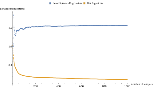
Figure 2: Comparison of the proposed method with ordinary least squares.

Appendix A Proofs Omitted from the Main Text

In this section we present all the formal proofs that are omitted from the main text. We start with some concentration results and some auxiliary lemmas that will be useful for the presentation of the missing proofs.

A.1 Useful Concentration Results

The following lemma is useful in cases where one wants to show concentration of a weighted sum of i.i.d sub-gamma random variables.

Definition 3.

(Sub-Gamma Random Variables) A random variable $x$ is called sub-gamma random variable if it satisfies

$$\log\left(\mathbb{E}\left[\exp(\lambda x)\right]\right)\leq\frac{\lambda^{2}v}{2(1-c\lambda)}~{}~{}~{}~{}\forall\lambda\in\left[0,\nicefrac{{1}}{{c}}\right]$$

for some positive constants $v,c$. We call $\Gamma_{+}(v,c)$ the set of all sub-gamma random variables.

Theorem 4 (Section 2.4 of [BLM13].).

Let $x^{(1)}$, …, $x^{(n)}$ be i.i.d. random variables such that $x^{(i)}\in\Gamma_{+}(v,c)$, $\boldsymbol{a}\in\mathbb{R}_{+}^{d}$. Then, the following inequalities hold for any $t\in\mathbb{R}_{+}$.

$$\mathbb{P}\left(\sum_{i=1}^{d}a_{i}\left(x^{(i)}-\mathbb{E}\left[x^{(i)}\right]\right)\geq\left\|\boldsymbol{a}\right\|_{2}\sqrt{2vt}+\left\|\boldsymbol{a}\right\|_{\infty}ct\right)\leq\exp(-t),$$

$$\mathbb{P}\left(-\sum_{i=1}^{d}a_{i}\left(x^{(i)}-\mathbb{E}\left[x^{(i)}\right]\right)\geq\left\|\boldsymbol{a}\right\|_{2}\sqrt{2vt}+\left\|\boldsymbol{a}\right\|_{\infty}ct\right)\leq\exp(-t).$$

We also need a matrix concentration inequality analog to the Bernstein inequality for real valued random variables. For a proof of this inequality we refer to Section 6.2 of [Tro12].

Theorem 5 (Theorem 6.2 of [Tro12]).

Consider a finite sequence $\{\boldsymbol{Z}_{i}\}$ of independent, random, self-adjoint matrices with dimension $k$. Assume that

$$\mathbb{E}\left[\boldsymbol{Z}_{i}\right]=\boldsymbol{0}\quad\text{and}\quad\mathbb{E}\left[\boldsymbol{Z}_{i}^{p}\right]\preceq\frac{p!}{2}\cdot R^{p-2}\boldsymbol{A}_{i}^{2}\quad\text{for $p=2,3,4,\dots$.}$$

Compute the variance parameter

$$\sigma^{2}:=\left\|\sum_{i}\boldsymbol{A}_{i}^{2}\right\|.$$

Then the following chain of inequalities holds for all $t\geq 0$.

$$\mathbb{P}\left(\lambda_{\max}\left(\sum_{i}\boldsymbol{Z}_{i}\right)\geq t\right) \leq k\cdot\exp\left(\frac{-t^{2}/2}{\sigma^{2}+Rt}\right)$$ (i)

$$\leq\begin{cases}k\cdot\exp(-t^{2}/4\sigma^{2})&\text{for $t\leq\sigma^{2}/R$;}\\ k\cdot\exp(-t/4R)&\text{for $t\geq\sigma^{2}/R$.}\end{cases}$$ (ii)

A.2 Auxiliary Lemmas

The following lemma will be useful in the proof of lemma 5.

Lemma 8.

Let $z$ be a random variable that follows a truncated Gaussian distribution $\mathcal{N}(0,1,S)$ with survival probability $a$ then there exists a real value $q>0$ such that

1. $q\leq 2\log\left(\nicefrac{{2}}{{a}}\right)$,

2. the random variable $z^{2}-q$ is stochastically dominated by a sub-gamma random variable $u\in\Gamma_{+}\left(1,2\right)$ with $\mathbb{E}[u]=\nicefrac{{1}}{{2}}$.

Proof.

We will prove that the random variable $z$ stochastically dominated by an exponential random variable. First observe that the distribution of $z^{2}$ for different sets $S$ is stochastically dominated from the distribution pf $z^{2}$ when $S=S^{*}=S_{q}=\{z\mid z^{2}\geq q\}$, where q is chosen such that $\mathcal{N}(0,1;S^{*})=a$. To prove this let $F_{S}$ be the cumulative distribution function of $z^{2}$ when the truncation set is $S$, we have that $\mathcal{N}(0,1;S)=\mathcal{N}(0,1;S^{*})=a$ and hence

$$\mathbb{P}_{z\sim\mathcal{N}(0,1,S)}\left(z^{2}\geq t\right)=\frac{1}{a}\mathcal{N}(0,1;S\cap S_{t}),$$

$$\mathbb{P}_{z\sim\mathcal{N}(0,1,S^{*})}\left(z^{2}\geq t\right)=\frac{1}{a}\mathcal{N}(0,1;S^{*}\cap S_{t}).$$

We now prove that $\mathcal{N}(0,1;S\cap S_{t})\leq\mathcal{N}(0,1;S^{*}\cap S_{t})$. If $t\geq q$ then $S^{*}\cap S_{t}=S_{t}$ and hence $S\cap S_{t}\subseteq S^{*}\cap S_{t}$ which implies $\mathcal{N}(0,1;S\cap S_{t})\leq\mathcal{N}(0,1;S^{*}\cap S_{t})$. If $t\leq q$ then $S^{*}\cap S_{t}=S^{*}$ and hence

$$\mathcal{N}(0,1;S^{*}\cap S_{t})=\mathcal{N}(0,1;S^{*})=\mathcal{N}(0,1;S)\geq\mathcal{N}(0,1;S\cap S_{t}).$$

Therefore $\mathcal{N}(0,1;S\cap S_{t})\leq\mathcal{N}(0,1;S^{*}\cap S_{t})$ and this implies $F_{S}(t)\geq F_{S^{*}}(t)$, which implies that the distribution of $z^{2}$ for different sets $S$ is stochastically dominated from the distribution pf $z^{2}$ when $S=S^{*}$. Hence we can focus on the distribution of $z^{2}$ when $z\sim\mathcal{N}(0,1,S^{*})$. First we have to get an upper bound on $q$. To do so we consider the $Q$-function of the standard normal distribution and we have that $a=\mathcal{N}(0,1;S^{*})=2Q(\sqrt{q})$. But by Chernoff bound we have that $Q(\sqrt{q})\leq\exp\left(-\nicefrac{{q}}{{2}}\right)$ which implies

$$q\leq 2\log\left(\frac{2}{a}\right).$$

Let $F_{z}$ the cumulative density function of $z$ and $F_{z^{2}}$ the cumulative density function of $z^{2}$, we have that

$$F_{z^{2}}(t)=F_{z}(\sqrt{t})-F_{z}(-\sqrt{t}),$$

but we know that

$$F_{z}(t)=\frac{1}{a}\begin{cases}\Phi(t)&~{}~{}~{}~{}~{}t\leq-\sqrt{q}\\ \Phi(-\sqrt{q})&~{}~{}~{}~{}~{}-\sqrt{q}<t<\sqrt{q}\\ \Phi(t)-(\Phi(\sqrt{q})-\Phi(-\sqrt{q}))&~{}~{}~{}~{}~{}t\geq\sqrt{q}\end{cases}$$

Hence we have that

$$F_{z^{2}}(t)=\frac{1}{a}\begin{cases}0&~{}~{}~{}~{}~{}t<q\\ \Phi(\sqrt{t})-\Phi(-\sqrt{t})-(\Phi(\sqrt{q})-\Phi(-\sqrt{q}))&~{}~{}~{}~{}~{}t\geq q\end{cases}$$

But we know that $\Phi(\sqrt{t})-\Phi(-\sqrt{t})$ is the cumulative density function of the square of a Gaussian distribution, namely is a gamma distribution with both parameters equal to $\nicefrac{{1}}{{2}}$. This means that $\Phi(\sqrt{t})-\Phi(-\sqrt{t})=\int_{0}^{t}\frac{\exp\left(-\nicefrac{{\tau}}{{2}}\right)}{\sqrt{2\pi\tau}}d\tau$ and hence we get

$$F_{z^{2}}(t)=\frac{1}{a}\begin{cases}0&~{}~{}~{}~{}~{}t<q\\ \int_{q}^{t}\frac{\exp\left(-\nicefrac{{\tau}}{{2}}\right)}{\sqrt{2\pi\tau}}d\tau&~{}~{}~{}~{}~{}t\geq q\end{cases}$$

If we define the random variable $v=z^{2}-q$ then the cumulative density function $F_{v}$ of $v$ is equal to

$$F_{v}(t)=\frac{1}{a}\int_{0}^{t}\frac{\exp\left(-\nicefrac{{\tau+q}}{{2}}\right)}{\sqrt{2\pi(\tau+q)}}d\tau$$

which implies that the probability density function $f_{v}$ of $v$ is equal to

$$f_{v}(t)=\frac{1}{a}\frac{\exp\left(-\nicefrac{{(t+q)}}{{2}}\right)}{\sqrt{2\pi(t+q)}}d\tau.$$

It is easy to see that the density of $f_{v}$ is stochastically dominated from the density of the exponential distribution $g(t)=\frac{1}{2}\exp\left(-\frac{x}{2}\right)$. The reason is that $f_{v}(t)$ and $g(t)$ are single crossing and $g(t)$ dominates when $t\to\infty$. Then it is easy to see that for the cumulative it holds that $G(t)\leq F_{v}(t)$. Hence $G(t)$ stochastically dominates $F_{v}(t)$. Finally we have that $G(t)$ is a sub-gamma $\Gamma_{+}(1,2)$ and hence $v$ is also sub-gamma $\Gamma_{+}(1,2)$ and the claim follows. ∎

The following lemma lower bounds the variance of $z\sim\mathcal{N}(\boldsymbol{w}^{T}\boldsymbol{x},1,S)$, and will be useful for showing strong convexity of the log likelihood for all values of the parameters in the projection set.

Lemma 9.

Let $\boldsymbol{x}\in\mathbb{R}^{k}$, $\boldsymbol{w}\in\mathbb{R}^{k}$, and $z\sim\mathcal{N}(\boldsymbol{w}^{T}\boldsymbol{x},1,S)$ then

$$\mathbb{E}\left[\left(z-\mathbb{E}\left[z\right]\right)^{2}\right]\geq\frac{\alpha(\boldsymbol{w},\boldsymbol{x})^{2}}{12}.$$

Proof.

We want to bound the following expectation: $\lambda_{1}=\mathbb{E}_{\boldsymbol{x}\sim\mathcal{N}(\boldsymbol{0},\boldsymbol{I},S)}[(x_{1}-\mu_{S,1})^{2}]=\mathrm{Var}_{\boldsymbol{x}\sim\mathcal{N}(\boldsymbol{0},\boldsymbol{I},S)}[g_{1}]$, where $g_{1}$ denotes the marginal distribution of $g$ along the direction of $\boldsymbol{e_{1}}$. Since $\mathcal{N}(\boldsymbol{0},\boldsymbol{I};S)=\alpha$, the worst case set (i.e the one that minimizes $\mathrm{Var}[g_{1}]$) is the one that has $\alpha$ mass as close as possible to the hyperplane $x_{1}=\mu_{S,1}$. However, the maximum mass that a gaussian places at the set $\{x_{1}:|x_{1}-\mu_{S,1}|<c\}$ is at most $2c$ as the density of the univariate gaussian is at most $1$. Thus the $\mathbb{E}_{\boldsymbol{x}\sim\mathcal{N}(\boldsymbol{0},\boldsymbol{I},S)}[(x_{1}-\mu_{S,1})^{2}]$ is at least the variance of the uniform distribution $U[-\alpha/2,\alpha/2]$ which is $\alpha^{2}/12$. Thus $\lambda_{i}\geq\lambda_{1}\geq\alpha^{2}/12$. ∎

A.3 Proof of Lemma 2

We have that

$$\alpha(\boldsymbol{w},\boldsymbol{x}) =\mathbb{E}_{y\sim\mathcal{N}(\boldsymbol{w}^{T}\boldsymbol{x},\boldsymbol{I})}[\mathds{1}_{y\in S}]$$

$$=\mathbb{E}_{y\sim\mathcal{N}(\boldsymbol{w}^{\prime T}\boldsymbol{x},\boldsymbol{I})}[\mathds{1}_{y\in S}\exp(\left\|y-\boldsymbol{w}^{\prime T}x\right\|^{2}/2-\left\|y-\boldsymbol{w}^{T}x\right\|^{2}/2)]$$

$$=\alpha(\boldsymbol{w}^{\prime},\boldsymbol{x})\cdot\mathbb{E}_{y\sim\mathcal{N}(\boldsymbol{w}^{\prime T}\boldsymbol{x},1,S)}[\exp(\frac{1}{2}\left\|y-\boldsymbol{w}^{\prime T}x\right\|^{2}-\frac{1}{2}\left\|y-\boldsymbol{w}^{T}x\right\|^{2})]$$

$$\geq\alpha(\boldsymbol{w}^{\prime},\boldsymbol{x})\cdot\exp(\mathbb{E}_{y\sim\mathcal{N}(\boldsymbol{w}^{\prime T}\boldsymbol{x},1,S)}[\frac{1}{2}\left\|y-\boldsymbol{w}^{\prime T}x\right\|^{2}-\frac{1}{2}\left\|y-\boldsymbol{w}^{T}x\right\|^{2}])$$

$$\geq\alpha(\boldsymbol{w}^{\prime},\boldsymbol{x})\cdot\exp(\mathbb{E}_{y\sim\mathcal{N}(\boldsymbol{w}^{\prime T}\boldsymbol{x},1,S)}[-\frac{1}{2}\left\|y-\boldsymbol{w}^{\prime T}x\right\|^{2}-\left|\left(\boldsymbol{w}-\boldsymbol{w}^{\prime}\right)^{T}\boldsymbol{x}\right|^{2}])$$

$$\geq\exp\left(-\left|\left(\boldsymbol{w}-\boldsymbol{w}^{\prime}\right)^{T}\boldsymbol{x}\right|^{2}-2\log\left(\frac{1}{\alpha(\boldsymbol{w}^{\prime},\boldsymbol{x})}\right)-2\right).$$

which implies the desired bound. The first inequality follows from Jensen’s inequality. The second follows from the fact that $\left\|u-v\right\|^{2}\leq 2\left\|u\right\|^{2}+2\left\|v\right\|^{2}$. The final inequality follows from Lemma 3. The same way we can prove the second part of the lemma.

A.4 Proof of Lemma 3

Let $\alpha(\boldsymbol{w},\boldsymbol{x})=c$ for some fixed constant $c<1$. Note that, $\mathcal{N}(\boldsymbol{w}^{T}\boldsymbol{x},1,S)$ is a truncated version of the normal distribution $\mathcal{N}(\boldsymbol{w}^{T}\boldsymbol{x},1)$. Assume, without loss of generality that $\boldsymbol{w}^{T}\boldsymbol{x}=0$. Our goal is to upper bound the second moment of this distribution around $0$. It is clear that for this moment to be maximized, we need to choose a set $S$ of measure $c$ that is located as far from $\mu$ as possible. Thus, the worst case set $S=(-\infty,-z]\cup[z,\infty)$ consists of both tails of $\mathcal{N}(0,\boldsymbol{I})$, each having mass $c/2$. We know that for the CDF of the normal distribution, the following holds:

$$\Phi(z)\geq 1-e^{-\frac{z^{2}}{2}}$$

and we need to find the point $z$ such that $\Phi(z)=1-\frac{c}{2}$. Thus, we have:

$$\frac{c}{2}\leq e^{-\frac{z^{2}}{2}}\Leftrightarrow z\leq\sqrt{2\log\left(\frac{2}{c}\right)}$$

It remains to upper bound $\mathbb{E}_{y\sim\mathcal{N}(0,1,S)}\left[(y-\boldsymbol{w}^{T}\boldsymbol{x})^{2}\right]$.

For the aforementioned worst case set $S$, this quantity is equal to the second non-central moment around $\boldsymbol{w}\boldsymbol{x}$ of the truncated Gaussian distribution in the interval $[z,\infty)$. Thus,

$$\mathbb{E}_{y\sim\mathcal{N}(0,1,S)}\left[(y-\boldsymbol{w}^{T}\boldsymbol{x})^{2}\right]=1+\frac{z\phi(z)}{1-\Phi(z)}$$

The term $M(z)=\frac{\phi(z)}{1-\Phi(z)}$ is the inverse Mills ratio which is bounded by $z\leq M(z)\leq z+1/z$ for $z>0$, see [Gor41].

Thus, $z^{2}+1\leq\mathbb{E}_{y\sim\mathcal{N}(0,1,S)}\left[(y-\boldsymbol{w}^{T}\boldsymbol{x})^{2}\right]\leq z^{2}+2\leq 2\log\left(\frac{2}{c}\right)+2$.

A.5 Proof of Lemma 4

Using the second part of Lemma 2 we have that for every $\boldsymbol{w}\in\mathcal{D}_{r^{*},\bar{B}}$ it holds that

$$\log\left(\frac{1}{\alpha(\boldsymbol{w},\boldsymbol{x}^{(i)})}\right) \leq 2\log\left(\frac{1}{\alpha(\boldsymbol{w},\boldsymbol{x}^{(j)})}\right)+\left|\boldsymbol{w}^{T}\left(\boldsymbol{x}^{(i)}-\boldsymbol{x}^{(j)}\right)\right|^{2}+2$$

if we also we the fact that $\left\|\boldsymbol{x}^{(i)}\right\|_{2}\leq 1$ and $\left\|\boldsymbol{w}\right\|_{2}\leq\bar{B}$, from (4.1) and Definition 2 we get that

$$\log\left(\frac{1}{\alpha(\boldsymbol{w},\boldsymbol{x}^{(j)})}\right) \geq\frac{1}{2}\log\left(\frac{1}{\alpha(\boldsymbol{w},\boldsymbol{x}^{(i)})}\right)-\bar{B}-1.$$ (A.1)

Using the first part of Lemma 2 we have that

$$\log\left(\frac{1}{\alpha(\boldsymbol{w},\boldsymbol{x}^{(i)})}\right) \leq 2\log\left(\frac{1}{\alpha(\boldsymbol{w}^{*},\boldsymbol{x}^{(i)})}\right)+\left|\left(\boldsymbol{w}-\boldsymbol{w}^{*}\right)^{T}\boldsymbol{x}^{(i)}\right|^{2}+2$$

$$\leq 2\log\left(\frac{1}{\alpha(\boldsymbol{w}^{*},\boldsymbol{x}^{(i)})}\right)+\left|y^{(i)}-\boldsymbol{w}^{T}\boldsymbol{x}^{(i)}\right|^{2}+\left|y^{(i)}-\boldsymbol{w}^{*T}\boldsymbol{x}^{(i)}\right|^{2}+2$$

Let now $\boldsymbol{v}\in\mathbb{R}^{k}$ be any unit vector, then we can multiply the above inequality by $\left(\boldsymbol{v}^{T}\boldsymbol{x}^{(i)}\right)^{2}$ and sum over all $i\in[n]$ and we get that

$$\sum_{i=1}^{n}\left(\boldsymbol{v}^{T}\boldsymbol{x}^{(i)}\right)^{2}\log\left(\frac{1}{\alpha(\boldsymbol{w},\boldsymbol{x}^{(i)})}\right) \leq 2\sum_{i=1}^{n}\left(\boldsymbol{v}^{T}\boldsymbol{x}^{(i)}\right)^{2}\log\left(\frac{1}{\alpha(\boldsymbol{w}^{*},\boldsymbol{x}^{(i)})}\right)+$$

$$~{}~{}~{}~{}~{}~{}~{}~{}+\sum_{i=1}^{n}\left(\boldsymbol{v}^{T}\boldsymbol{x}^{(i)}\right)^{2}\left|y^{(i)}-\boldsymbol{w}^{T}\boldsymbol{x}^{(i)}\right|^{2}+$$

$$~{}~{}~{}~{}~{}~{}~{}~{}+\sum_{i=1}^{n}\left(\boldsymbol{v}^{T}\boldsymbol{x}^{(i)}\right)^{2}\left|y^{(i)}-\boldsymbol{w}^{*T}\boldsymbol{x}^{(i)}\right|^{2}+2$$

now we can use the fact that $$\boldsymbol{w}\in\mathcal{D}_{r^{*},\bar{B}} \boldsymbol{w}^{*}\in\mathcal{D}_{r^{*},\bar{B}}$$, , and Assumption 1 to get

$$\sum_{i=1}^{n}\frac{\left(\boldsymbol{v}^{T}\boldsymbol{x}^{(i)}\right)^{2}}{\sum_{j=1}^{n}\left(\boldsymbol{v}^{T}\boldsymbol{x}^{(j)}\right)^{2}}\log\left(\frac{1}{\alpha(\boldsymbol{w},\boldsymbol{x}^{(i)})}\right) \leq 2\log\left(\frac{1}{a}\right)+2r^{*}+2.$$

Now fix some $$\ell\in[n] \ell i i$$, using (A.1) for the indices and for all in the above inequality we get that

$$\frac{1}{2}\log\left(\frac{1}{\alpha(\boldsymbol{w},\boldsymbol{x}^{(\ell)})}\right) \leq 2\log\left(\frac{1}{a}\right)+2r^{*}+3+\bar{B}$$

from which the lemma follows.

A.6 Proof of Lemma 5

By our assumption we have that bounded $\ell_{2}$ norm condition of $\mathcal{D}_{r^{*},\bar{B}}$ is satisfied. So our goal next is to prove that the first condition is satisfied too. Hence, we have to prove that

$$\frac{1}{n}\sum_{i=1}^{n}\left(\boldsymbol{\varepsilon}^{(i)}\right)^{2}\boldsymbol{x}^{(i)}\boldsymbol{x}^{(i)T}\preceq r\frac{1}{n}\sum_{i=1}^{n}\boldsymbol{x}^{(i)}\boldsymbol{x}^{(i)T},$$

where $\boldsymbol{\varepsilon}^{(i)}=y^{(i)}-\boldsymbol{w}^{*T}\boldsymbol{x}^{(i)}$ and $r=\log\left(\nicefrac{{1}}{{a}}\right)$. Observe that $\boldsymbol{\varepsilon}^{(i)}$ is a truncated standard normal random variable with the following truncation set

$$S^{(i)}=\left\{\boldsymbol{z}\mid\left(\boldsymbol{z}+\boldsymbol{w}^{*T}\boldsymbol{x}^{(i)}\right)\in S\right\}.$$

Therefore we have to prove that for any unit vector $\boldsymbol{v}$ it holds that

$$\frac{1}{n}\sum_{i=1}^{n}\left(\boldsymbol{\varepsilon}^{(i)}\right)^{2}\left(\boldsymbol{v}^{T}\boldsymbol{x}^{(i)}\right)^{2}\leq r\cdot\frac{1}{n}\sum_{i=1}^{n}\left(\boldsymbol{v}^{T}\boldsymbol{x}^{(i)}\right)^{2}.$$

For start we fix a unit vector $\boldsymbol{v}$ and we want to bound the following probability

$$\mathbb{P}\left(\frac{1}{n}\sum_{i=1}^{n}\left(\boldsymbol{\varepsilon}^{(i)}\right)^{2}\left(\boldsymbol{v}^{T}\boldsymbol{x}^{(i)}\right)^{2}\geq t\cdot\frac{1}{n}\sum_{i=1}^{n}\left(\boldsymbol{v}^{T}\boldsymbol{x}^{(i)}\right)^{2}\right).$$

This means that we are interested in the independent random variables $\left(\boldsymbol{\varepsilon}^{(i)}\right)^{2}$. Let $q^{(i)}$ the real value that is guaranteed to exist from Lemma 8 and corresponds to $\boldsymbol{\varepsilon}^{(i)}$ and $\boldsymbol{u}^{(i)}$ the corresponding random variable guaranteed to exist from Lemma 8. We also define $\boldsymbol{\delta}^{(i)}=\left(\boldsymbol{\varepsilon}^{(i)}\right)^{2}-q^{(i)}$, finally set $a^{(i)}=\alpha(\boldsymbol{w}^{*},\boldsymbol{x}^{(i)})$. We have that

$$\frac{1}{n}\sum_{i=1}^{n}\left(\boldsymbol{\varepsilon}^{(i)}\right)^{2}\left(\boldsymbol{v}^{T}\boldsymbol{x}^{(i)}\right)^{2} \leq 2\frac{1}{n}\sum_{i=1}^{n}\boldsymbol{\delta}^{(i)}\left(\boldsymbol{v}^{T}\boldsymbol{x}^{(i)}\right)^{2}+2\frac{1}{n}\sum_{i=1}^{n}q^{(i)}\left(\boldsymbol{v}^{T}\boldsymbol{x}^{(i)}\right)^{2}$$

$$\leq 2\frac{1}{n}\sum_{i=1}^{n}\boldsymbol{\delta}^{(i)}\left(\boldsymbol{v}^{T}\boldsymbol{x}^{(i)}\right)^{2}+4\frac{1}{n}\sum_{i=1}^{n}\log\left(\frac{2}{a^{(i)}}\right)\left(\boldsymbol{v}^{T}\boldsymbol{x}^{(i)}\right)^{2}$$

but from Assumption 1 this implies

$$\leq 2\frac{1}{n}\sum_{i=1}^{n}\boldsymbol{\delta}^{(i)}\left(\boldsymbol{v}^{T}\boldsymbol{x}^{(i)}\right)^{2}+4\log\left(\frac{2}{a}\right).$$

Now the random variables $\boldsymbol{\delta}^{(i)}$ are stochastically dominated by $\boldsymbol{u}^{(i)}$ and hence

$$\mathbb{P}\left(\frac{1}{n}\sum_{i=1}^{n}\boldsymbol{\delta}^{(i)}\left(\boldsymbol{v}^{T}\boldsymbol{x}^{(i)}\right)^{2}\geq t\cdot\frac{1}{n}\sum_{i=1}^{n}\left(\boldsymbol{v}^{T}\boldsymbol{x}^{(i)}\right)^{2}\right)\leq\mathbb{P}\left(\frac{1}{n}\sum_{i=1}^{n}\boldsymbol{u}^{(i)}\left(\boldsymbol{v}^{T}\boldsymbol{x}^{(i)}\right)^{2}\geq t\cdot\frac{1}{n}\sum_{i=1}^{n}\left(\boldsymbol{v}^{T}\boldsymbol{x}^{(i)}\right)^{2}\right)$$

But from the fact that $\mathbb{E}\left[\boldsymbol{u}^{(i)}\right]=1/2$ we have that

$$\frac{1}{n}\sum_{i=1}^{n}\boldsymbol{u}^{(i)}\left(\boldsymbol{v}^{T}\boldsymbol{x}^{(i)}\right)^{2} \leq\frac{1}{n}\sum_{i=1}^{n}\left(\boldsymbol{u}^{(i)}-\mathbb{E}\left[\boldsymbol{u}^{(i)}\right]\right)\left(\boldsymbol{v}^{T}\boldsymbol{x}^{(i)}\right)^{2}+\frac{1}{n}\sum_{i=1}^{n}\left(\boldsymbol{v}^{T}\boldsymbol{x}^{(i)}\right)^{2}$$

Therefore we have that

$$\mathbb{P}\left(\frac{\sum_{i=1}^{n}\left(\boldsymbol{\varepsilon}^{(i)}\right)^{2}\left(\boldsymbol{v}^{T}\boldsymbol{x}^{(i)}\right)^{2}}{\sum_{i=1}^{n}\left(\boldsymbol{v}^{T}\boldsymbol{x}^{(i)}\right)^{2}}\geq t+4\log\left(\nicefrac{{2}}{{a}}\right)+1\right)\leq\mathbb{P}\left(\frac{\sum_{i=1}^{n}\left(\boldsymbol{u}^{(i)}-\mathbb{E}\left[\boldsymbol{u}^{(i)}\right]\right)\left(\boldsymbol{v}^{T}\boldsymbol{x}^{(i)}\right)^{2}}{\sum_{i=1}^{n}\left(\boldsymbol{v}^{T}\boldsymbol{x}^{(i)}\right)^{2}}\geq t\right).$$ (A.2)

To bound the last probability we will use the matrix analog of Bernstein’s inequality as we expressed in Theorem 5. More precisely we will bound the following probability

$$\mathbb{P}\left(\lambda_{\max}\left(\sum_{i=1}^{n}\left(\boldsymbol{u}^{(i)}-\mathbb{E}\left[\boldsymbol{u}^{(i)}\right]\right)\boldsymbol{x}^{(i)}\boldsymbol{x}^{(i)T}\right)\geq t\cdot\lambda_{\max}\left(\sum_{i=1}^{n}\boldsymbol{x}^{(i)}\boldsymbol{x}^{(i)T}\right)\right).$$

We set $\boldsymbol{Z}_{i}=\frac{1}{n\cdot\lambda_{\max}(\boldsymbol{X})}\left(\boldsymbol{u}^{(i)}-\mathbb{E}\left[\boldsymbol{u}^{(i)}\right]\right)\boldsymbol{x}^{(i)}\boldsymbol{x}^{(i)T}$, where $\boldsymbol{X}=\frac{1}{n}\sum_{i=1}^{n}\boldsymbol{x}^{(i)}\boldsymbol{x}^{(i)T}$. Observe that

$$\left(\boldsymbol{x}^{(i)}\boldsymbol{x}^{(i)T}\right)^{p}=\left\|\boldsymbol{x}^{(i)}\right\|_{2}^{2(p-2)}\left(\boldsymbol{x}^{(i)}\boldsymbol{x}^{(i)T}\right)^{2}.$$

Also since $\boldsymbol{u}^{(i)}$ is an exponential random variable with parameter $1/2$, it is well known that

$$\mathbb{E}\left[\left(\boldsymbol{u}^{(i)}-\mathbb{E}\left[\boldsymbol{u}^{(i)}\right]\right)^{p}\right]\leq\frac{p!}{2}2^{p}.$$

These two relations imply that

$$\mathbb{E}\left[\boldsymbol{Z}_{i}^{p}\right]\preceq\frac{p!}{2}\left(2\cdot\frac{1}{\lambda_{\max}(\boldsymbol{X})}\cdot\frac{\left\|\boldsymbol{x}^{(i)}\right\|_{2}^{2}}{n}\right)^{p-2}\cdot\left(\frac{1}{\lambda_{\max}(\boldsymbol{X})}\cdot\frac{2}{n}\boldsymbol{x}^{(i)}\boldsymbol{x}^{(i)T}\right)^{2}$$

Hence we can apply Theorem 5 with $R=2\cdot\frac{1}{\lambda_{\max}(\boldsymbol{X})}\cdot\frac{\left\|\boldsymbol{x}^{(i)}\right\|_{2}^{2}}{n}$ and $\boldsymbol{A}_{i}=\frac{1}{\lambda_{\max}(\boldsymbol{X})}\cdot\frac{2}{n}\boldsymbol{x}^{(i)}\boldsymbol{x}^{(i)T}$. Now observe that by Assumption 1 we get that

$$\frac{\left\|\boldsymbol{x}^{(i)}\right\|_{2}^{2}}{n}\leq\frac{\lambda_{\max}(\boldsymbol{X})}{\log k}.$$

We now compute the variance parameter

$$\sigma^{2}=\left\|\sum_{i=1}^{n}\boldsymbol{A}_{i}\right\|=4\cdot\frac{1}{\lambda_{\max}(\boldsymbol{X})}\cdot\frac{\left\|\boldsymbol{x}^{(i)}\right\|_{2}^{2}}{n}\left\|\frac{1}{n}\sum_{i=1^{n}}\boldsymbol{x}^{(i)}\right\|\boldsymbol{x}^{(i)T}\leq\frac{4}{\log k}.$$

Using the same reasoning we get $R\leq 2/\log k$, therefore applying Theorem 5 we get that

$$\mathbb{P}\left(\lambda_{\max}\left(\sum_{i=1}^{n}\boldsymbol{Z}_{i}\geq t\right)\right) \leq k\exp\left(-\frac{t^{2}}{2\sigma^{2}+Rt}\right)$$

$$\leq k\exp\left(-\frac{t^{2}\log k}{8+2t}\right)$$

From the last inequality we get that for $t\geq 5$ there is at most probability $1/3$ such that

$$\mathbb{P}\left(\lambda_{\max}\left(\sum_{i=1}^{n}\left(\boldsymbol{u}^{(i)}-\mathbb{E}\left[\boldsymbol{u}^{(i)}\right]\right)\boldsymbol{x}^{(i)}\boldsymbol{x}^{(i)T}\right)\geq t\cdot\lambda_{\max}(\boldsymbol{X})\right)\leq\frac{1}{3}$$

and hence the lemma follows.

A.7 Proof of Theorem 3

We now use our Lemmas 2, 3, 5 to prove some useful inequalities that we need to prove our strong convexity and bounded step variance.

Lemma 10.

Let $(\boldsymbol{x}^{(1)},y^{(i)}),\dots,(\boldsymbol{x}^{(n)},y^{(n)})$ be $n$ samples from the linear regression model (3.1) with parameters $\boldsymbol{w}^{*}$. If Assumptions 1 and 1 hold, and if $\left\|\boldsymbol{x}^{(i)}\right\|_{2}\leq 1$ for all $i\in[n]$ then

$$\frac{1}{n}\sum_{i=1}^{n}\left\|((\boldsymbol{w}-\boldsymbol{w}^{*})^{T}\boldsymbol{x}^{(i)})\boldsymbol{x}^{(i)}\right\|_{2}^{2}\leq 2\cdot\bar{B}^{2},$$ (A.3)

$$\frac{1}{n}\sum_{i=1}^{n}\mathbb{E}\left[\left\|(y^{(i)}-\boldsymbol{w}^{*T}\boldsymbol{x}^{(i)})\boldsymbol{x}^{(i)}\right\|_{2}^{2}\right]\leq 2\log\left(\frac{1}{a}\right)+4,$$ (A.4)

$$\frac{1}{n}\sum_{i=1}^{n}\mathbb{E}\left[\left\|(z^{(i)}-\boldsymbol{w}^{T}\boldsymbol{x}^{(i)})\boldsymbol{x}^{(i)}\right\|_{2}^{2}\right]\leq r^{*}+2\cdot\bar{B}^{2},$$ (A.5)

where $y^{(i)}\sim\mathcal{N}(\boldsymbol{w}^{*T}\boldsymbol{x}^{(i)},1,S)$, $z^{(i)}\sim\mathcal{N}(\boldsymbol{w}^{T}\boldsymbol{x}^{(i)},1,S)$ and $\boldsymbol{w}\in\mathcal{D}_{r^{*},\bar{B}}$ with $r^{*}=4\log\left(\nicefrac{{2}}{{a}}\right)+7$.

Proof.

We prove one by one the above inequalities.

Proof of (A.3). Since $\boldsymbol{w},\boldsymbol{w}^{*}\in\mathcal{D}_{r^{*},\bar{B}}$ we have that $\left\|\boldsymbol{w}-\boldsymbol{w}^{*}\right\|_{2}\leq 2\bar{B}$. If we combine this with the assumption that $\left\|\boldsymbol{x}^{(i)}\right\|_{2}\leq 1$ and the fact that $\left\|\boldsymbol{z}\right\|_{2}\leq\left\|\boldsymbol{z}\right\|_{\infty}\cdot\sqrt{k}$ then we get that

$$\frac{1}{n}\sum_{i=1}^{n}\left\|((\boldsymbol{w}-\boldsymbol{w}^{*})^{T}\boldsymbol{x}^{(i)})\boldsymbol{x}^{(i)}\right\|_{2}^{2}\leq 2\cdot B^{2}\cdot k.$$

Proof of (A.4). Using Lemma 3 we get that

$$\frac{1}{n}\sum_{i=1}^{n}\mathbb{E}\left[\left\|(y^{(i)}-\boldsymbol{w}^{*T}\boldsymbol{x}^{(i)})\boldsymbol{x}^{(i)}\right\|_{2}^{2}\right]\leq\frac{1}{n}\sum_{i=1}^{n}\left(2\log\left(\frac{1}{\alpha(\boldsymbol{w}^{*T},\boldsymbol{x}^{(i)})}\right)+4\right)\left\|\boldsymbol{x}^{(i)}\right\|_{2}^{2}$$

but now we can use Assumption 1 and the assumption that $\left\|\boldsymbol{x}^{(i)}\right\|_{2}\leq 1$ and we get that

$$\frac{1}{n}\sum_{i=1}^{n}\mathbb{E}\left[\left\|(y^{(i)}-\boldsymbol{w}^{*T}\boldsymbol{x}^{(i)})\boldsymbol{x}^{(i)}\right\|_{2}^{2}\right]\leq 2\log\left(\frac{1}{a}\right)+4.$$

Proof of (A.5). Using Lemma 3 we get that

$$\frac{1}{n}\sum_{i=1}^{n}\mathbb{E}\left[\left\|(z^{(i)}-\boldsymbol{w}^{T}\boldsymbol{x}^{(i)})\boldsymbol{x}^{(i)}\right\|_{2}^{2}\right]\leq\frac{1}{n}\sum_{i=1}^{n}\left(2\log\left(\frac{1}{\alpha(\boldsymbol{w},\boldsymbol{x}^{(i)})}\right)+4\right)\left\|\boldsymbol{x}^{(i)}\right\|_{2}^{2}.$$

Using Lemma 2 on the last inequality we get that

$$\frac{1}{n}\sum_{i=1}^{n}\mathbb{E}\left[\left\|(z^{(i)}-\boldsymbol{w}^{T}\boldsymbol{x}^{(i)})\boldsymbol{x}^{(i)}\right\|_{2}^{2}\right] \leq\frac{1}{n}\sum_{i=1}^{n}\left(2\log\left(\frac{1}{\alpha(\boldsymbol{w}^{*},\boldsymbol{x}^{(i)})}\right)+4\right)\left\|\boldsymbol{x}^{(i)}\right\|_{2}^{2}+$$

$$~{}~{}~{}+\frac{1}{n}\sum_{i=1}^{n}\left\|((\boldsymbol{w}-\boldsymbol{w}^{*})^{T}\boldsymbol{x}^{(i)})\boldsymbol{x}^{(i)}\right\|_{2}^{2}+2$$

Now using (A.3), Assumption 1, and the facts that $$\left\|\boldsymbol{x}^{(i)}\right\|_{2}\leq 1 \left\|\boldsymbol{w}-\boldsymbol{w}^{*}\right\|_{2}\leq 2\bar{B}$$ and we get that

$$frac{1}{n}\sum_{i=1}^{n}\mathbb{E}\left[\left\|(z^{(i)}-\boldsymbol{w}^{T}\boldsymbol{x}^{(i)})\boldsymbol{x}^{(i)}\right\|_{2}^{2}\right] \leq 2\log\left(\frac{1}{a}\right)+4+2\cdot\bar{B}^{2}$$

$$\leq r^{*}+2\cdot\bar{B}^{2}.$$

∎

Given Lemma 10 we are now ready to prove Theorem 3.

Proof of Theorem 3.

We first prove (4.13) and then (4.14).

Proof of (4.13). Using the fact that $\left\|\boldsymbol{x}^{(i)}\right\|_{2}\leq 1$ we get that

$$\mathbb{E}\left[\left\|y^{(i)}\boldsymbol{x}^{(i)}-z^{(j)}\boldsymbol{x}^{(j)}\right\|_{2}^{2}\right] \leq\mathbb{E}\left[\left\|y^{(i)}\boldsymbol{x}^{(i)}\right\|_{2}^{2}+\left\|z^{(j)}\boldsymbol{x}^{(j)}\right\|_{2}^{2}\right]\leq\mathbb{E}\left[\left(y^{(i)}\right)^{2}\right]+\frac{1}{n}\sum_{j\in[n]}\mathbb{E}\left[\left(z^{(j)}\right)^{2}\right]$$

$$\leq\mathrm{Var}\left[y^{(i)}\right]+\left(\mathbb{E}[y^{(i)}]\right)^{2}+\frac{1}{n}\sum_{j\in[n]}\left(\mathrm{Var}\left[z^{(j)}\right]+\left(\mathbb{E}[z^{(j)}]\right)^{2}\right)$$

Now we can use the fact that $y^{(i)}\sim\mathcal{N}(\boldsymbol{w}^{*T}\boldsymbol{x}^{(i)},1,S)$ and that $z^{(j)}\sim\mathcal{N}(\boldsymbol{w}^{T}\boldsymbol{x}^{(j)},1,S)$ together with Lemma 6 from [DGTZ18] and the fact $\left\|\boldsymbol{x}^{(i)}\right\|_{2}\leq 1$ we get that

$$\mathbb{E}\left[\left\|y^{(i)}\boldsymbol{x}^{(i)}-z^{(j)}\boldsymbol{x}^{(j)}\right\|_{2}^{2}\right] \leq 2\left\|\boldsymbol{w}^{*}\right\|^{2}_{2}+3\log\left(\frac{1}{\alpha(\boldsymbol{w}^{*},\boldsymbol{x}^{(i)})}\right)+2\left\|\boldsymbol{w}\right\|^{2}_{2}+\frac{3}{n}\sum_{j\in[n]}\log\left(\frac{1}{\alpha(\boldsymbol{w},\boldsymbol{x}^{(j)})}\right)$$

Now using Lemma 4 and the fact that $\left\|\boldsymbol{w}^{*}\right\|_{2}\leq\bar{B}$ and $\left\|\boldsymbol{w}\right\|_{2}\leq\bar{B}$ we get that

$$\mathbb{E}\left[\left\|y^{(i)}\boldsymbol{x}^{(i)}-z^{(j)}\boldsymbol{x}^{(j)}\right\|_{2}^{2}\right] \leq O(\mathrm{poly}(1/a)\cdot\bar{B}^{2})$$

from which (4.13) follows.

Proof of (4.14). Let $\boldsymbol{v}$ be an arbitrary unit vector in $\mathbb{R}^{k}$. Using Lemma 9 from Appendix A.2 and then the first part of Lemma 2, we have that

$$\frac{1}{n}\sum_{i=1}^{n}\mathbb{E}\left[\left(z^{(i)}-\mathbb{E}\left[z^{(i)}\right]\right)^{2}\right] \left(\boldsymbol{v}^{T}\boldsymbol{x}^{(i)}\right)^{2}\geq\frac{1}{n}\sum_{i=1}^{n}\alpha^{2}(\boldsymbol{w},\boldsymbol{x}^{(i)})\left(\boldsymbol{v}^{T}\boldsymbol{x}^{(i)}\right)^{2}$$

$$\geq\frac{e^{-2}}{n}\sum_{i=1}^{n}\exp\left(-\left\|(\boldsymbol{w}-\boldsymbol{w}^{*})^{T}\boldsymbol{x}^{(i)}\right\|_{2}^{2}-2\log\left(\frac{1}{\alpha(\boldsymbol{w}^{*},\boldsymbol{x}^{(i)})}\right)\right)\cdot$$

$$~{}~{}~{}~{}~{}~{}~{}~{}~{}~{}~{}~{}~{}~{}~{}~{}\cdot\left(\boldsymbol{v}^{T}\boldsymbol{x}^{(i)}\right)^{2}$$

now we can divide both sides with $$\frac{1}{n}\sum_{i=1}^{n}\left(\boldsymbol{v}^{T}\boldsymbol{x}^{(i)}\right)^{2}$$ and then apply Jensen’s inequality and we get

$$\frac{1}{\frac{1}{n}\sum_{i=1}^{n}\left(\boldsymbol{v}^{T}\boldsymbol{x}^{(i)}\right)^{2}}\frac{1}{n} \sum_{i=1}^{n}\mathbb{E}\left[\left(z^{(i)}-\mathbb{E}\left[z^{(i)}\right]\right)^{2}\right]\left(\boldsymbol{v}^{T}\boldsymbol{x}^{(i)}\right)^{2}$$

$$\geq\exp\left(-\frac{\sum_{i=1}^{n}\left(\left\|(\boldsymbol{w}-\boldsymbol{w}^{*})^{T}\boldsymbol{x}^{(i)}\right\|_{2}^{2}+2\log\left(\frac{1}{\alpha(\boldsymbol{w}^{*},\boldsymbol{x}^{(i)})}\right)\right)\left(\boldsymbol{v}^{T}\boldsymbol{x}^{(i)}\right)^{2}}{\sum_{i=1}^{n}\left(\boldsymbol{v}^{T}\boldsymbol{x}^{(i)}\right)^{2}}\right)$$

now applying Assumption 1 we get

$$\geq a^{2}\exp\left(-\frac{\sum_{i=1}^{n}\left\|(\boldsymbol{w}-\boldsymbol{w}^{*})^{T}\boldsymbol{x}^{(i)}\right\|_{2}^{2}\left(\boldsymbol{v}^{T}\boldsymbol{x}^{(i)}\right)^{2}}{\sum_{j=1}^{n}\left(\boldsymbol{v}^{T}\boldsymbol{x}^{(i)}\right)^{2}}\right)$$

$$\geq a^{2}\exp\left(-\frac{\sum_{i=1}^{n}\left\|y^{(i)}-\boldsymbol{w}^{*T}\boldsymbol{x}^{(i)}\right\|_{2}^{2}\left(\boldsymbol{v}^{T}\boldsymbol{x}^{(i)}\right)^{2}}{\sum_{j=1}^{n}\left(\boldsymbol{v}^{T}\boldsymbol{x}^{(i)}\right)^{2}}\right)\cdot$$

$$~{}~{}~{}~{}~{}~{}~{}~{}~{}~{}~{}\cdot\exp\left(-\frac{\sum_{i=1}^{n}\left\|y^{(i)}-\boldsymbol{w}^{T}\boldsymbol{x}^{(i)}\right\|_{2}^{2}\left(\boldsymbol{v}^{T}\boldsymbol{x}^{(i)}\right)^{2}}{\sum_{j=1}^{n}\left(\boldsymbol{v}^{T}\boldsymbol{x}^{(i)}\right)^{2}}\right)$$

now we can use the fact the both $\boldsymbol{w}$ and $\boldsymbol{w}^{*}$ belong to the projection set $\mathcal{D}_{r^{*},B}$ as we showed in Lemma 5 and we get

$$\frac{1}{\frac{1}{n}\sum_{i=1}^{n}\left(\boldsymbol{v}^{T}\boldsymbol{x}^{(i)}\right)^{2}}\frac{1}{n}\sum_{i=1}^{n}\mathbb{E}\left[\left(z^{(i)}-\mathbb{E}\left[z^{(i)}\right]\right)^{2}\right]\left(\boldsymbol{v}^{T}\boldsymbol{x}^{(i)}\right)^{2}\geq a^{2}\exp\left(-2r^{*}\right)$$

and using Assumption 1 the relation (4.14) follows. ∎

Appendix B Efficient Sampling of Truncated Gaussian with Union of Intervals Survival Set

In this section, in Lemma 13, we see that when $S=\cup_{i=1}^{r}[a_{i},b_{i}]$, with $a_{i},b_{i}\in\mathbb{R}$, then we can efficiently sample from the truncated normal distribution $\mathcal{N}(\mu,\sigma,S)$ in time $\mathrm{poly}(n,k)$ even under the weak bound on the mass of the set $\mathcal{N}(\mu,\sigma;S)\geq a^{\mathrm{poly}(n,k)}$. The only difference is that instead of exact sampling we have approximate sampling, but the approximation error is exponentially small in total variation distance and hence it cannot affect any algorithm that runs in poly-time.

Definition 4 (Evaluation Oracle).

Let $f:\mathbb{R}\to\mathbb{R}$ be an arbitrary real function. We define the evaluation oracle $\mathcal{E}_{f}$ of $f$ as an oracle that given a number $x\in\mathbb{R}$ and a target accuracy $\eta$ computes an $\eta$-approximate value of $f(x)$, that is $\left|\mathcal{E}_{f}(x)-f(x)\right|\leq\eta$.

Lemma 11.

Let $f:\mathbb{R}\to\mathbb{R}_{+}$ be a real increasing and differentiable function and $\mathcal{E}_{f}(x)$ an evaluation oracle of $f$. Let $\ell\leq f^{\prime}(x)\leq L$ for some $\ell,L\in\mathbb{R}_{+}$. Then we can construct an algorithm that implements the evaluation oracle of $f^{-1}$, i.e. $\mathcal{E}_{f^{-1}}$. This implementation on input $y\in\mathbb{R}_{+}$ and input accuracy $\eta$ runs in time $T$ and uses at most $T$ calls to the evaluation oracle $\mathcal{E}_{f}$ with inputs $x$ with representation length $T$ and input accuracy $\eta^{\prime}=\eta/\ell$, with $T=\mathrm{poly}\log(\max\{|f(0)/y|,|y/f(0)|\},L,1/\ell,1/\eta)$.

Proof of Lemma 11.

Given a value $y\in\mathbb{R}_{+}$ our goal is to find an $x\in\mathbb{R}$ such that $f(x)=y$. Using doubling we can find two numbers $a,b$ such that $f(a)\leq y-\eta^{\prime}$ and $f(b)\geq y+\eta^{\prime}$ for some $\eta^{\prime}$ to be determined later. Because of the lower bound $\ell$ on the derivative of $f$ we have that this step will take $\log((1/\ell)\cdot\max\{|f(0)/y|,|y/f(0)|\})$ steps. Then we can use binary search in the interval $[a,b]$ where in each step we make a call to the oracle $\mathcal{E}_{f}$ with accuracy $\eta^{\prime}$ and we can find a point $\hat{x}$ such that $\left|f(x)-f(\hat{x})\right|\leq\eta^{\prime}$. Because of the upper bound on the derivative of $f$ we have that $f$ is $L$-Lipschitz and hence this binary search will need $\log(L/\eta^{\prime})$ time and oracle calls. Now using the mean value theorem we get that for some $\xi\in[a,b]$ it holds that $\left|f(x)-f(\hat{x})\right|=|f^{\prime}(\xi)|\left|x-\hat{x}\right|$ which implies that $\left|x-\hat{x}\right|\leq\eta^{\prime}/\ell$, so if we set $\eta^{\prime}=\ell\cdot\eta$, the lemma follows. ∎

Using the Lemma 11 and the Proposition 3 of [Che12] it is easy to prove the following lemma.

Lemma 12.

Let $[a,b]$ be a closed interval and $\mu\in\mathbb{R}$ such that $\gamma_{[a,b]}(\mu)=\alpha$. Then there exists an algorithm that runs in time $\mathrm{poly}\log(1/\alpha,\zeta)$ and returns a sample of a distribution $\mathcal{D}$, such that $d_{\mathrm{TV}}(\mathcal{D},N(\mu,1;[a,b]))\leq\zeta$.

Proof Sketch.

The sampling algorithm follows the steps: (1) from the cumulative distribution function $F$ of the distribution $N(\mu,1;[a,b])$ define a map from $[a,b]$ to $[0,1]$, (2) sample uniformly a number $y$ in $[0,1]$ (3) using an evaluation oracle for the error function, as per Proposition 3 in [Che12], and using Lemma 11 compute with exponential accuracy the value $F^{-1}(y)$ and return this as the desired sample. ∎

Finally using again Proposition 3 in [Che12] and Lemma 12 we can get the following lemma.

Lemma 13.

Let $[a_{1},b_{1}]$, $[a_{2},b_{2}]$, $\dots$, $[a_{r},b_{r}]$ be closed intervals and $\mu\in\mathbb{R}$ such that $\gamma_{\cup_{i=1}^{r}[a_{i},b_{i}]}(\mu)=\alpha$. Then there exists an algorithm that runs in time $\mathrm{poly}(\log(1/\alpha,\zeta),r)$ and returns a sample of a distribution $\mathcal{D}$, such that $d_{\mathrm{TV}}(\mathcal{D},N(\mu,1;\cup_{i=1}^{r}[a_{i},b_{i}]))\leq\zeta$.

Proof Sketch.

Using Proposition 3 in [Che12] we can compute $\hat{\alpha}_{i}$ which estimated with exponential accuracy the mass $\alpha_{i}=\gamma_{[a_{i},b_{i}]}(\mu)$ of every interval $[a_{i},b_{i}]$. If $\hat{\alpha}_{i}/\alpha\leq\zeta/3r$ then do not consider interval $i$ in the next step. From the remaining intervals we can choose one proportionally to $\hat{\alpha}_{i}$. Because of the high accuracy in the computation of $\hat{\alpha}_{i}$ this is $\zeta/3$ close in total variation distance to choosing an interval proportionally to $\alpha_{i}$. Finally after choosing an interval $i$ we can run the algorithm of Lemma 12 with accuracy $\zeta/3$ and hence the overall total variation distance from $N(\mu,1;\cup_{i=1}^{r}[a_{i},b_{i}])$ is at most $\zeta$. ∎

References

- [Ame73] Takeshi Amemiya. Regression analysis when the dependent variable is truncated normal. Econometrica: Journal of the Econometric Society, pages 997–1016, 1973.
- [BC14] N Balakrishnan and Erhard Cramer. The art of progressive censoring. Springer, 2014.
- [BDLS17] Sivaraman Balakrishnan, Simon S. Du, Jerry Li, and Aarti Singh. Computationally efficient robust sparse estimation in high dimensions. In Proceedings of the 30th Conference on Learning Theory, COLT 2017, Amsterdam, The Netherlands, 7-10 July 2017, pages 169–212, 2017.
- [BJK15] Kush Bhatia, Prateek Jain, and Purushottam Kar. Robust regression via hard thresholding. In Advances in Neural Information Processing Systems, pages 721–729, 2015.
- [BLC13] Yoshua Bengio, Nicholas Léonard, and Aaron Courville. Estimating or propagating gradients through stochastic neurons for conditional computation. arXiv preprint arXiv:1308.3432, 2013.
- [BLM13] Stéphane Boucheron, Gábor Lugosi, and Pascal Massart. Concentration inequalities: A nonasymptotic theory of independence. Oxford university press, 2013.
- [Bre96] Richard Breen. Regression models: Censored, sample selected, or truncated data, volume 111. Sage, 1996.
- [Che12] Sylvain Chevillard. The functions erf and erfc computed with arbitrary precision and explicit error bounds. Information and Computation, 216:72–95, 2012.
- [CLMW11] Emmanuel J Candès, Xiaodong Li, Yi Ma, and John Wright. Robust principal component analysis? Journal of the ACM (JACM), 58(3):11, 2011.
- [Coh16] A Clifford Cohen. Truncated and censored samples: theory and applications. CRC press, 2016.
- [CSV17] Moses Charikar, Jacob Steinhardt, and Gregory Valiant. Learning from untrusted data. In Proceedings of the 49th Annual ACM SIGACT Symposium on Theory of Computing, STOC 2017, Montreal, QC, Canada, June 19-23, 2017, pages 47–60, 2017.
- [DGTZ18] Constantinos Daskalakis, Themis Gouleakis, Christos Tzamos, and Manolis Zampetakis. Efficient statistics, in high dimensions, from truncated samples. In the 59th Annual IEEE Symposium on Foundations of Computer Science (FOCS), 2018.
- [DKK+16] Ilias Diakonikolas, Gautam Kamath, Daniel M. Kane, Jerry Li, Ankur Moitra, and Alistair Stewart. Robust estimators in high dimensions without the computational intractability. In IEEE 57th Annual Symposium on Foundations of Computer Science, FOCS 2016, 9-11 October 2016, Hyatt Regency, New Brunswick, New Jersey, USA, pages 655–664, 2016.
- [DKK+17] Ilias Diakonikolas, Gautam Kamath, Daniel M. Kane, Jerry Li, Ankur Moitra, and Alistair Stewart. Being robust (in high dimensions) can be practical. In Proceedings of the 34th International Conference on Machine Learning, ICML 2017, Sydney, NSW, Australia, 6-11 August 2017, pages 999–1008, 2017.
- [DKK+18] Ilias Diakonikolas, Gautam Kamath, Daniel M. Kane, Jerry Li, Ankur Moitra, and Alistair Stewart. Robustly learning a gaussian: Getting optimal error, efficiently. In Proceedings of the Twenty-Ninth Annual ACM-SIAM Symposium on Discrete Algorithms, SODA 2018, New Orleans, LA, USA, January 7-10, 2018, pages 2683–2702, 2018.
- [DKS19] Ilias Diakonikolas, Weihao Kong, and Alistair Stewart. Efficient algorithms and lower bounds for robust linear regression. In the 30th Annual ACM-SIAM Symposium on Discrete Algorithms (SODA), 2019.
- [Fis31] RA Fisher. Properties and applications of Hh functions. Mathematical tables, 1:815–852, 1931.
- [Gal97] Francis Galton. An examination into the registered speeds of american trotting horses, with remarks on their value as hereditary data. Proceedings of the Royal Society of London, 62(379-387):310–315, 1897.
- [GLS12] Martin Grötschel, László Lovász, and Alexander Schrijver. Geometric algorithms and combinatorial optimization, volume 2. Springer Science & Business Media, 2012.
- [GMDB16] Caglar Gulcehre, Marcin Moczulski, Misha Denil, and Yoshua Bengio. Noisy activation functions. In International Conference on Machine Learning, pages 3059–3068, 2016.
- [Gor41] Robert D Gordon. Values of mills’ ratio of area to bounding ordinate and of the normal probability integral for large values of the argument. The Annals of Mathematical Statistics, 12(3):364–366, 1941.
- [HM13] Moritz Hardt and Ankur Moitra. Algorithms and hardness for robust subspace recovery. In Conference on Learning Theory, pages 354–375, 2013.
- [Hot48] Harold Hotelling. Fitting generalized truncated normal distributions. In Annals of Mathematical Statistics, volume 19, pages 596–596, 1948.
- [HW77] Jerry A Hausman and David A Wise. Social experimentation, truncated distributions, and efficient estimation. Econometrica: Journal of the Econometric Society, pages 919–938, 1977.
- [Li17] Jerry Li. Robust sparse estimation tasks in high dimensions. CoRR, abs/1702.05860, 2017.
- [LRV16] Kevin A. Lai, Anup B. Rao, and Santosh Vempala. Agnostic estimation of mean and covariance. In IEEE 57th Annual Symposium on Foundations of Computer Science, FOCS 2016, 9-11 October 2016, Hyatt Regency, New Brunswick, New Jersey, USA, pages 665–674, 2016.
- [Mad86] Gangadharrao S Maddala. Limited-dependent and qualitative variables in econometrics. Cambridge university press, 1986.
- [NH10] Vinod Nair and Geoffrey E Hinton. Rectified linear units improve restricted boltzmann machines. In Proceedings of the 27th international conference on machine learning (ICML-10), pages 807–814, 2010.
- [NJN19] Dheeraj Nagaraj, Prateek Jain, and Praneeth Netrapalli. Sgd without replacement: Sharper rates for general smooth convex functions. In International Conference on Machine Learning, pages 4703–4711, 2019.
- [Pea02] Karl Pearson. On the systematic fitting of frequency curves. Biometrika, 2:2–7, 1902.
- [PL08] Karl Pearson and Alice Lee. On the generalised probable error in multiple normal correlation. Biometrika, 6(1):59–68, 1908.
- [PVRB18] Loucas Pillaud-Vivien, Alessandro Rudi, and Francis Bach. Statistical optimality of stochastic gradient descent on hard learning problems through multiple passes. In Advances in Neural Information Processing Systems, pages 8114–8124, 2018.
- [Sch86] Helmut Schneider. Truncated and censored samples from normal populations. Marcel Dekker, Inc., 1986.
- [SCV18] Jacob Steinhardt, Moses Charikar, and Gregory Valiant. Resilience: A criterion for learning in the presence of arbitrary outliers. In 9th Innovations in Theoretical Computer Science Conference, ITCS 2018, January 11-14, 2018, Cambridge, MA, USA, pages 45:1–45:21, 2018.
- [Sha16] Ohad Shamir. Without-replacement sampling for stochastic gradient methods. In Advances in neural information processing systems, pages 46–54, 2016.
- [Tob58] James Tobin. Estimation of relationships for limited dependent variables. Econometrica: journal of the Econometric Society, pages 24–36, 1958.
- [Tro12] Joel A Tropp. User-friendly tail bounds for sums of random matrices. Foundations of computational mathematics, 12(4):389–434, 2012.
- [Tuk49] John W Tukey. Sufficiency, truncation and selection. The Annals of Mathematical Statistics, pages 309–311, 1949.
- [XCM10] Huan Xu, Constantine Caramanis, and Shie Mannor. Principal component analysis with contaminated data: The high dimensional case. arXiv preprint arXiv:1002.4658, 2010.