MTAG: Modal-Temporal Attention Graph for
Unaligned Human Multimodal Language Sequences

Abstract

Human communication is multimodal in nature; it is through multiple modalities such as language, voice, and facial expressions, that opinions and emotions are expressed. Data in this domain exhibits complex multi-relational and temporal interactions. Learning from this data is a fundamentally challenging research problem. In this paper, we propose Modal-Temporal Attention Graph (MTAG). MTAG is an interpretable graph-based neural model that provides a suitable framework for analyzing multimodal sequential data. We first introduce a procedure to convert unaligned multimodal sequence data into a graph with heterogeneous nodes and edges that captures the rich interactions across modalities and through time. Then, a novel graph fusion operation, called MTAG fusion, along with a dynamic pruning and read-out technique, is designed to efficiently process this modal-temporal graph and capture various interactions. By learning to focus only on the important interactions within the graph, MTAG achieves state-of-the-art performance on multimodal sentiment analysis and emotion recognition benchmarks, while utilizing significantly fewer model parameters.

1 Introduction

Figure 1: Example visualization of tri-modal Modal-Temporal Attention learned by our proposed model. Each circle represents a node from video/text/audio modalities, and the blue lines denote the learned attention weights (i.e. the thicker and darker a blue line is, the larger the attention weight). We observe high intensities between semantically correlated graph entities, such as "Really Enjoy" and the raise in eyebrow, which indicate positive sentiment. Note that our graph-based model learns multimodal interactions without prior alignment, and captures diverse types of interactions across multiple modalities all the same time. Edge types are not shown for visual clarity.

With recent advances in machine learning research, analysis of multimodal sequential data has become increasingly prominent. At the core of modeling this form of data, there are the fundamental research challenges of fusion and alignment. Fusion is the process of blending information from multiple modalities. It is usually preceded by alignment, which is the process of finding temporal relations between the modalities. An important research area that exhibits this form of data is multimodal language analysis, where sequential modalities of language, vision, and acoustic are present. These three modalities carry the communicative information and interact with each other through time; e.g. positive word at the beginning of an utterance may be the cause of a smile at the end.

Figure 2: The 3-stage MTAG framework: Node Construction, Edge Construction and Fusion+Pruning. [Node Construction] Each modality’s features are first passed through a distinct Feed-Forward-Network to be mapped into the same embedding size. Then, a positional embedding is added to each transformed feature based on its position in its own modality, so that temporal information are encoded. The features are now nodes in the graph. [Edge Construction] We then apply an algorithm to construct edges among these nodes by appropriately indexing each edge with a modal type and a temporal type. [Fusion+Pruning] Finally, we pass the graph into the MTAG module to learn interactions across modality and time. The output graph with updated node embeddings and pruned edges can be passed to downstream modules, e.g. a Multi-layer Perceptron, to complete specific tasks such as regression or classification.

When analyzing such multimodal sequential data, it is crucial to build models that perform both fusion and alignment accurately and efficiently by a) aligning arbitrarily distributed asynchronous modalities in an interpretable manner, b) efficiently accounting for short and long-range dependencies, c) explicitly modeling the inter-modal interactions between the modalities while simultaneously accounting for intra-modal dynamics.

In this paper, we propose MTAG (Modal-Temporal Attention Graph). MTAG is capable of both fusion and alignment of asynchronously distributed multimodal sequential data. Modalities do not need to be pre-aligned, nor do they need to follow similar sampling rate. MTAG can capture interactions of various types across any number of modalities all at once, comparing to previous methods that model bi-modal interactions at a time Tsai et al. (2019a). At its core, MTAG utilizes an efficient trimodal-temporal graph fusion operation. Coupled with our proposed dynamic pruning technique, MTAG learns a parameter-efficient and interpretable graph. In our experiments, we use two unaligned multimodal emotion recognition and sentiment analysis benchmarks: IEMOCAP Busso et al. (2008) and CMU-MOSI Zadeh et al. (2016). The proposed MTAG model achieves state-of-the-art performance with far fewer parameters. Subsequently, we visualize the learned relations between modalities and explore the underlying dynamics of multimodal language data. Our model incorporates all three modalities in both alignment and fusion, a fact that is also substantiated in our ablation studies.

2 Related Works

Human Multimodal Language Analysis

Analyzing human multimodal language involves learning from data across multiple heterogeneous sources that are often asynchronous, i.e. language, visual, and acoustic modalities that each uses a different sampling rate. Earlier works assumed multimodal sequences are aligned based on word boundaries Lazaridou et al. (2015); Ngiam et al. (2011); Gu et al. (2018); Dumpala et al. (2019); Pham et al. (2019) and applied fusion methods for aligned sequences. To date, modeling unaligned multimodal language sequences remains understudied, except for Tsai et al. (2019a); Khare et al. (2020); Zheng et al. (2020), which used cross-modal Transformers to model unaligned multimodal language sequences. However, the cross-modal Transformer module is a bi-modal operation that only account for two modalities’ input at a time. In Tsai et al. (2019a), the authors used multiple cross-modal Transformers and applies late fusion to obtain tri-modal features, resulting in a large amount of parameters needed to retain original modality information. Other works that also used cross-modal Transformer architecture for include Yang et al. (2020); Siriwardhana et al. (2020). In contrast to the existing works, our proposed graph method, with very small amount of model parameters, can aggregate information from multiple (more than 2) modalities at early stage by building edges between the corresponding modalities, allowing richer and more complex representation of the interactions to be learned.

Graph Neural Networks

Graph Neural Network (GNN) was introduced in Gori et al. (2005); Scarselli et al. (2008) with an attempt to extend deep neural networks to handle graph-structured data. Since then, there has been an increasing research interest on generalizing deep neural network’s operations such as convolution Kipf and Welling (2016); Schlichtkrull et al. (2017); Hamilton et al. (2017), recurrence (Nicolicioiu et al., 2019), and attention Veličković et al. (2018) to graph.

Recently, several heterogeneous GNN methods Wang et al. (2019a); Wei et al. (2019); Shi et al. (2016) have been proposed. The heterogeneous nodes referred in these works consist of uni-modal views of multiple data generating sources (such as movie metadata node, audience metadata node, etc.), whereas in our case the graph nodes represent multimodal views of a single data generating source (visual, acoustic, textual nodes from a single speaking person). In the NLP domain, multimodal GNN methods Khademi (2020); Yin et al. (2020) on tasks such as Visual Question Answering and Machine Translation. However, these settings still differ from ours because they focused on static images and short text which, unlike the multimodal video data in our case, do not exhibit long-term temporal dependencies across modalities.

Based on these findings, we discovered there has been little research using graph-based methods for modeling unaligned, multimodal language sequences, which includes video, audio and text. In this paper, we demonstrate our proposed MTAG method can effectively model such unaligned, multimodal sequential data.

3 MTAG

Notation	Explanation
$v_{i}$	Node $i$
$e_{ij}$	Edge from $v_{i}$ to $v_{j}$
$\mathbfcal{N}_{i}$	Neighbor nodes incident into $v_{i}$
${\mathbf{x}_{i}}$	Initial node feature for $v_{i}$
${\mathbf{x^{\prime}}_{i}}$	Transformed node feature for $v_{i}$
${\pi}_{i}$	Node type for $v_{i}$
${\phi}_{ij}$	Edge modality type for $e_{ij}$
${\tau}_{ij}$	Edge temporal type for $e_{ij}$
$\mathbf{M}_{\pi_{i}}$	Node type specific transformation matrix
$\mathbf{a}^{\phi_{ij},\tau_{ij}}$	Edge type specific learnable attention vector
$\beta_{i,j}$	Raw attention score of node pair ($v_{i}$,$v_{j}$)
$\alpha_{i,j}$	Attention weight of node pair ($v_{i}$,$v_{j}$),
	normalized over $\mathbfcal{N}_{i}$
${\mathbf{z}_{i}}$	Node output feature for $v_{i}$
$k$	Prune percentage
$h$	Index of multi-head attention head
$H$	Number of total attention heads

Table 1: Terminologies used in this paper.

In this section, we describe our proposed framework: Modal Temporal Attention Graph (MTAG) for unaligned multimodal language sequences. We describe how we formulate the multimodal data into a graph $\mathbfcal{G}(\mathbfcal{V},\mathbfcal{E})$, and the MTAG fusion operation that operates on $\mathbfcal{G}$. In essence, our graph formulation by design alleviates the need for any hard alignments, and combined with MTAG fusion, allows nodes from one modality to interact freely with nodes from all other modalities at the same time, breaking the limitation of only modeling pairwise modality interactions in previous works. Figure 2 gives a high-level overview of the framework.

3.1 Node Construction

As illustrated in Figure 2, each modality’s input feature vectors are first passed through a modality-specific Feed-Forward-Network. This allows feature embeddings from different modalities to be transformed into the same dimension. A positional embedding (details in Appendix A) is then added (separately for each modality) to each embedding to encode temporal information. The output of this operation becomes a node $v_{i}$ in the graph. Each node is marked with a modality identifier $\pi_{i}$, where $\pi_{i}\in\{\text{Audio, Video, Text}\}$ in our case.

3.2 Edge Construction

In this section, we describe our design of modality edges and temporal edges. For a given node of a particular modality, its interactions with nodes from different modalities should be considered differently. For example, given a Video node, its interaction with an Audio node should be different from that with a Text node. In addition, the temporal order of the nodes also plays a key role in multimodal analysis Poria et al. (2017). For example, a transition from a frown to a smile ( $\rightarrow$ $\rightarrow$ ) may imply a positive sentiment, whereas a transition from a smile to a frown ( $\rightarrow$ $\rightarrow$ ) may imply a negative sentiment. Therefore, interactions between nodes that appear in different temporal orders should also be considered differently. In GNNs, the edges define how node features are aggregated within a graph. In order to encapsulate the diverse types of node interactions, we assign edge types to each edge so that information can be aggregated differently on different types of edges. By indexing edges with edge types, different modal and temporal interactions between nodes can be addressed separately.

Multimodal Edges. As we make no assumption about prior alignment of the modalities, the graph is initialized to be a fully connected graph. We use $e_{ij}$ to represent an edge from $v_{i}$ to $v_{j}$. We assign $e_{ij}$ with a modality type identifier $\phi_{ij}=(\pi_{i}\rightarrow\pi_{j})$. For example, an edge pointing from a Video node to a Text node will be marked with type $\phi_{ij}=(\text{Video}\rightarrow\text{Text})$.

Temporal Edges. In addition to $\phi_{ij}$, we also assign a temporal label $\tau_{ij}$ to each $e_{ij}$. Depending on the temporal order of $v_{i}$ and $v_{j}$ connected by $e_{ij}$, we determine the value of $\tau_{ij}$ to be either of $\{\text{past, present, future}\}$. For nodes from the same modality, the temporal orders can be easily determined by comparing their order of occurrences. To determine the temporal orders for nodes across different modalities, we first roughly align the two modalities with our pseudo-alignment. Then the temporal order can be simply read out.

Pseudo-Alignment. As mentioned above, it is simple to determine the temporal edge types for nodes in a single modality. However, there is no clear definition of “earlier" or “later" across two modalities, due to the unaligned nature of our input sequences. To this end, we introduce the pseudo-alignment heuristic that coarsely defines the past, present and future connections between nodes across two modalities. Given a node $v_{i}$ from one modality $\pi_{i}$, our pseudo-alignment first determines a set of nodes $\mathbfcal{V}_{i,present}$ in the other modality that can be aligned to $v_{i}$ and considered as “present". All nodes in the other modality that exists after $\mathbfcal{V}_{i,present}$ are considered “future" $\mathbfcal{V}_{i,future}$, and all those before are considered $\mathbfcal{V}_{i,past}$. Once the coarse temporal order is established, the cross-modal temporal edge types can be easily determined. Figure 3 shows an example of such pseudo-alignment, and more details regarding the calculations can be found in Appendix A.2.

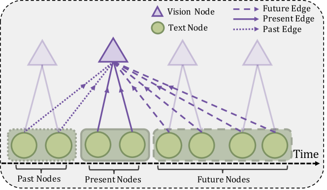
Figure 3: An example of the pseudo-alignment between two unaligned sequences. We first align the longer sequence to the shorter one as uniformly as possible. Then the aligned nodes from the longer sequence becomes the $\mathbfcal{V}_{i,present}$ for node $v_{i}$ in the shorter sequence. $\mathbfcal{V}_{i,past}$ and $\mathbfcal{V}_{i,future}$ can then be determined accordingly.

3.3 Fusion and Pruning

3.3.1 MTAG Fusion

With our formulation of the graph, we design the MTAG fusion operation that can digest our graph data with various node and edge types, and thus model the modal-temporal interactions. An algorithm of our method is shown in Algorithm 1 and a visual illustration is given in Figure 4. Specifically, for each neighbor node $v_{j}$ that has an edge incident into a center node $v_{i}$, we compute a raw attention score $\beta_{[h],i,j}$ based on that edge’s modality and temporal type:

$$\beta_{[h],i,j}=\text{LeakyRelu}(\mathbf{a}_{[h]}^{\phi_{ji},\tau_{ji}}\cdot[\mathbf{x}_{i}^{\prime}\|\mathbf{x}_{j}^{\prime}])$$ (1)

where $[\cdot||\cdot]$ denotes the concatenation of two column vectors into one long column vector. The $[h]$ index is used to distinguish which multi-head attention head is being used. Note that $\mathbf{a}_{[h]}^{\phi_{ji},\tau_{ji}}$ depends on both the modality and temporal edge types of $e_{ji}$. This results in 27 edge types (9 types of modality interaction $\times$ 3 types of temporal interaction).

We normalize the raw attention scores over all neighbor nodes $v_{j}$ with Softmax so that the normalized attention weight sums to 1 to preserve the scale of the node features in the graph.

$$\alpha_{[h],i,j}=\frac{\exp\bigl{(}\beta_{[h],i,j}\bigr{)}}{\sum_{k\in\mathbfcal{N}_{i}}\exp\bigl{(}\beta_{[h],i,k}\bigr{)}}$$ (2)

Then, we perform node feature aggregation for each node $v_{i}$ following:

$$\mathbf{z}_{i}=\operatorname*{concat}\limits_{h=1}^{H}(\sum_{j\in\mathbfcal{N}_{i}}\alpha_{[h],i,j}\mathbf{x}_{j}^{\prime})$$ (3)

where $\mathcal{N}_{i}$ defines the neighbors of $v_{i}$ and hyperparameter $H$ is the number of total attention heads. $\mathbf{z}_{i}$ now becomes the new node embedding for node $v_{i}$. After aggregation, $v_{i}$ transformed from a node with unimodal information into a node encoding the diverse modal-temporal interactions between $v_{i}$ and its neighbors (illustrated by the mixing of colors of the nodes in Figure 2).

1 Feature transformation $\mathbf{x}^{\prime}_{i}\leftarrow\mathbf{M}_{\pi_{i}}\mathbf{x}_{i},\forall i$

2

3for $h=1...H$ do

4       for $j\in\mathbfcal{N}_{i}\cup i$ do

5            

6            calculate raw attention score using modality- and temporal-edge-type specific parameters: $\beta_{[h],i,j}=\text{LeakyRelu}(\mathbf{a}_{[h]}^{\phi_{ji},\tau_{ji}}\cdot[\mathbf{x}_{i}^{\prime}\|\mathbf{x}_{j}^{\prime}])$

7      normalize raw attention scores over $\mathbfcal{N}_{i}\cup i$ to get attention weight $\alpha_{[h],i,j}$

8calculate node output feature $\mathbf{z}_{i}=\operatorname*{concat}\limits_{h=1}^{H}(\sum_{j\in\mathbfcal{N}_{i}\cup i}\alpha_{[h],i,j}\mathbf{x}_{j}^{\prime})$

9calculate average attention weight across all heads $\overline{\alpha}_{i,j}=\frac{1}{H}\sum_{h=1}^{H}(\alpha_{[h],i,j})$

10 sort $\overline{\alpha}_{i,j}$ and delete the edges with the smallest $k\%$ average attention weight from $\mathbfcal{N}_{i}\cup i$, obtaining $\mathbfcal{N}_{i}^{\prime}$

11return $\mathbf{z}_{i}$, $\mathbfcal{N}_{i}^{\prime}\ \ \forall i$

Algorithm 1 MTAG with edge pruning

We desgined the operation to have $H$ multi-head attention heads because the heterogeneous input data of the multimodal graph could be of different scales, making the variance of the data high. Adding multi-head attention could help stabilize the behavior of the operation.

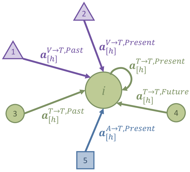
Figure 4: Visualization of the MTAG operation around a single node. The text on each edge indicates which attention vector is used for that edge. Purple triangle represents a video node, green circle represents a text node and blue square represents an audio node.

3.3.2 Dynamic Edge Pruning

Our graph formulation models interactions for all 27 edge types. This design results in a very large number of edges in the graph, making the computation graph difficult to fit into GPU memories. More importantly, when there are so many edges, it is hard to avoid some of these edges from inducing spurious correlations and distracting the model from focusing on the truly important interactions (Lee et al., 2019; Knyazev et al., 2019). To address these challenges, we propose to dynamically prune edges as the model learns the graph. Specifically, after each layer of MTAG, we have the attention weight $\alpha_{[h],i,j}$ for each attention head $h$ and for each edge $e_{ij}$. We take the average of the attention weights over the attention heads:

$$\overline{\alpha}_{ij}=\frac{1}{H}\sum_{h=1}^{H}(\alpha_{[h],i,j})$$ (4)

Then, we sort $\overline{\alpha}_{ij}$ and delete $k\%$ edges with the smallest attention weights, where $k$ is a hyperparameter. These deleted edges will no longer be calculated in the next MTAG fusion layer. Our ablation study in Section 5.2 empirically verifies the effectiveness of this approach by comparing to no pruning and random pruning.

3.4 Graph Readout

At the end of the MTAG fusion process, we need to read out information scattered in the nodes into a single vector so that we can pass it through a classification head. Recall that the pruning process drops edges in the graph. If all edges incident into a node have been dropped, then it means that node was not updated based on its neighbors. In that case, we simply ignore that node in the readout process.

We readout the graph by averaging all the surviving nodes’ output features into one vector. This vector is then passed to a 3-layer Multi-Layer-Perceptron (MLP) to make the final prediction.

4 Experiments

Model \ Emotion	Happy	Sad	Angry	Neutral
(Unaligned) IEMOCAP Emotions.
CTC + EF-LSTM	75.7	70.5	67.1	57.4
LF-LSTM	71.8	70.4	67.9	56.2
CTC + RAVEN	76.8	65.6	64.1	59.5
CTC + MCTN	77.5	71.7	65.6	49.3
MulT	81.9	74.1	70.2	59.7
MTAG (ours)	86.0	79.9	76.7	64.1

Table 2: F1 Scores on unaligned IEMOCAP. Higher is better.

We empirically evaluate MTAG model on two datasets: IEMOCAP Busso et al. (2008) and CMU-MOSI Zadeh et al. (2016); both are well-known datasets used by prior works (Liang et al., 2018; Pham et al., 2019; Tsai et al., 2019b, a) to benchmark multimodal emotion recognition and sentiment analysis.

4.1 Dataset and Metrics

IEMOCAP

IEMOCAP is a multimodal emotion recognition dataset consisting of 10K videos. The task we chose is the 4-way multilabel emotion classification, classifying into happy, sad, angry and neutral. For train split, the positive/negative label ratio for each emotion is 954:1763, 338:2379, 690:2027 and 735:1982. For the test split, the ratio is 383:555, 135:803, 193:745 and 227:711. Due to this unbalanced distribution of the the labels, we use F1 score as a better metric for comparison.

CMU-MOSI

CMU Multimodal Opinion Sentiment Intensity is a multimodal sentiment analysis dataset with 2,199 movie review video clips. Each video clip is labeled with real-valued sentiment score within $[-3,+3]$, with $+3$ being a very positive sentiment and $-3$ a very negative one. Following previous works Tsai et al. (2019a), we report five metrics: 7-class classification accuracy ($\text{Acc}_{7}$), binary classification accuracy ($\text{Acc}_{2}$, positive/negative sentiments), F1 score, Mean Absolute Error (MAE) and the correlation of the model’s prediction with human.

We follow prior works Tsai et al. (2019a) to evaluate on both of the above unaligned datasets, where original audio and video features are used, resulting in variable sequence lengths across modalities. For both datasets, the multimodal features are extracted from the textual (GloVe word embeddings Pennington et al. (2014)), visual (Facet iMotions (2017)), and acoustic (COVAREP Degottex et al. (2014)) data modalities.

Model \ Metirc	$\text{Acc}_{7}\uparrow$	$\text{Acc}_{2}\uparrow$	$\text{F1}\uparrow$	$\text{MAE}\downarrow$	$\text{Corr}\uparrow$
(Unaligned) CMU-MOSI Sentiment
CTC+EF-LSTM	31.0	73.6	74.5	1.078	0.542
LF-LSTM	33.7	77.6	77.8	0.988	0.624
CTC+MCTN	32.7	75.9	76.4	0.991	0.613
CTC+RAVEN	31.7	72.7	73.1	1.076	0.544
MulT	39.1	81.1	81.0	0.889	0.686
MTAG (ours)	38.9	82.3	82.1	0.866	0.722

Table 3: Results on unaligned CMU-MOSI. $\uparrow$ means higher is better and $\downarrow$ means lower is better.

Model	# Parameters
MulT (previous SOTA)	2.24 M
MTAG (ours)	0.14 M

Table 4: Number of model parameters (M = Million).

4.2 Baselines

For basleine evaluations, we use Early Fusion LSTM (EF-LSTM) and Late Fusion LSTM (LF-LSTM) (Tsai et al., 2019a) as baselines. In addition, we compare our model against similar methods as in previous works Tsai et al. (2019a), which combine a Connectionist Temporal Classification (CTC) loss Graves et al. (2006) with the pre-existing methods such as EF-LSTM, MCTN Pham et al. (2019), RAVEN Wang et al. (2019b).

4.3 Results

Shown in Table 2 and Table 3, MTAG substantially out-performs previous methods on unaligned IEMOCAP benchmark and CMU-MOSI benchmark on most of the metrics. MTAG also achieves on-par performance on the $\text{Acc}_{7}$ metric on CMU-MOSI benchmark. With an extremely small number of parameters, our model is able to learn better alignment and fusion for multimodal sentiment analysis task. Details regarding our model and hyper-parameters can be found in the Appendix A.

Parameter Efficiency (MTAG vs MulT)

We discover that MTAG is a highly parameter-efficient model. A comparison of model parameters between MTAG and MulT Tsai et al. (2019a) (previous state of the art) is shown in Table 4. The hyperparameter used for this comparison can be found in the Appendix. With only a fraction ($6.25\%$) of MulT’s parameters, MTAG is able to achieve on-par, and in most cases superior performance on the two datasets. This demonstrates the parameter efficiency of our method.

Qualitative Analysis

The attention weights on the graph edges forms a natural way to interpret our model. We visualize the edges to probe what MTAG has learned. The following case study is a randomly selected video clip from the CMU-MOSI validation set. We observe the phenomena shown below is a general trend.

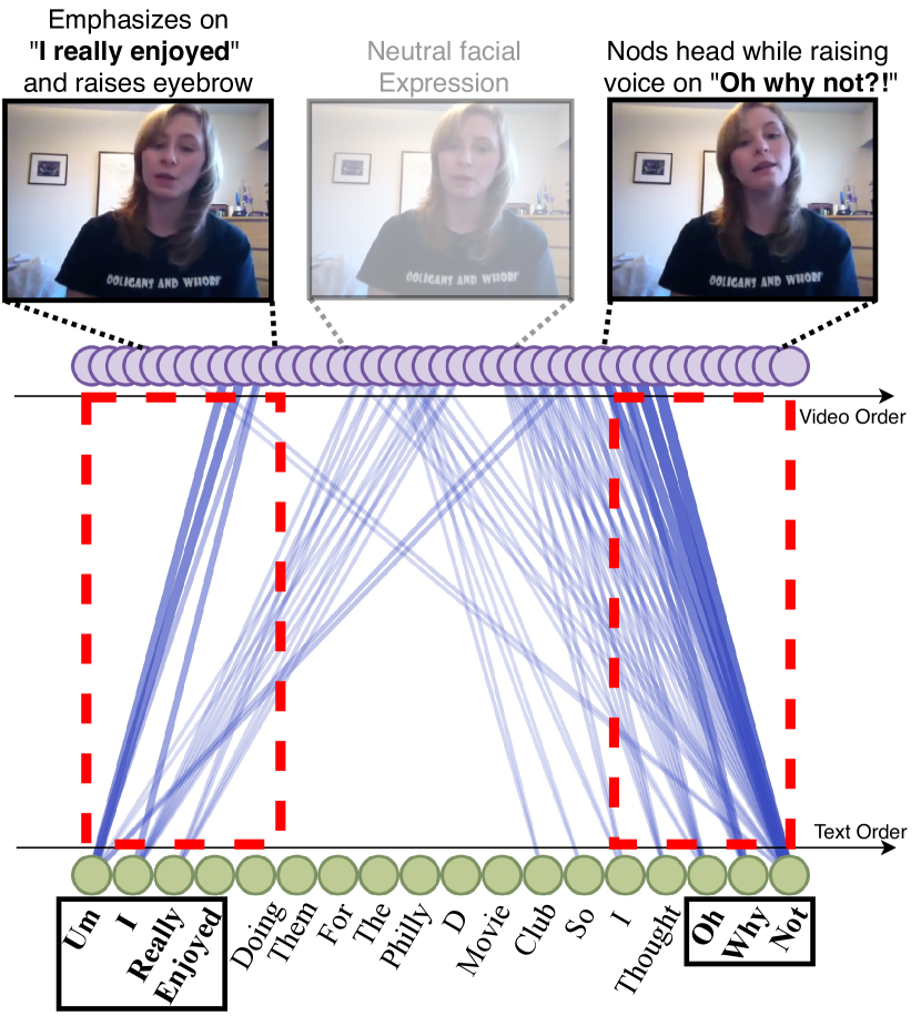
(a) Text-to-vision edge attention weights.

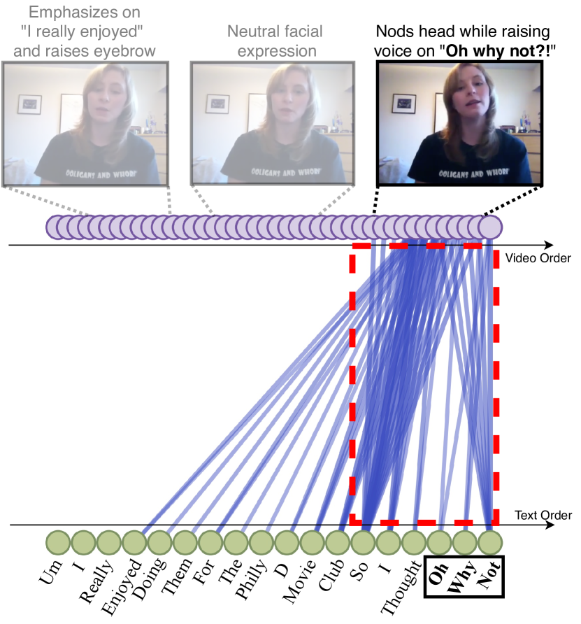
(b) Vision-to-text edge attention weights.

Figure 5: We visualized the asymmetric attention weights of the text-to-vision and vision-to-text edges for one of the validation sequence in CMU-MOSI dataset. The visualized attention weights are from layer 3 of MTAG. Note that the edge types are not shown here for visual clarity.

In Figure 5, we show an example of the asymmetric bi-modal relations between vision and text. We observe that our model picks on meaningful relations between words such as “I really enjoyed" and facial expressions such as raising eyebrow, highlighted in the red dashed boxes in Figure 5(a). Our model can also learn long-range correlation between “I really enjoyed" and head nodding. Interestingly, we discover that strong relations that are not detected by vision-to-text edges can be recovered by the text-to-vision edges. This advocates the design of the multi-type edges, which allows the model to learn different relations independently that can complement one another.

Figure 1 gives a holistic view of the attention weights among all three modalities. We observe a pattern where almost all edges involve the text modality. A possible explanation for this observation is that the text is the dominant modality with respect to the sentiment analysis task. This hypothesis is verified by the ablation study in Sec. 5.3. Meanwhile, there appears to be very small amount of edges connecting directly between vision and audio, indicating that there might be little meaningful correlation between them. This resonates with our ablation studies in Table 5, where vision and audio combined produce the lowest bi-modal performance. Under such circumstance, our MTAG learns to kill direct audio-vision relations and instead fuse their information indirectly using the text modality as a proxy, whereas previous methods such as MulT keeps audio-vision attentions alive along the way, introducing possible spurious relations that could distract model learning.

5 Ablation Study

We conduct ablation study using unalgined CMU-MOSI dataset. MTAG Full Model implements multimodal temporal edge types, adopts TopK edge pruning that keeps edges with top $80\%$ edge weights, and includes all three modalities as its input. Table 5 shows the performance. We present research questions (RQs) as follows and discuss how ablation studies address them.

5.1 RQ1: Does using 27 edge types help?

We first study the effect of edge types on our model performance. As we incrementally add in multimodal and temporal edge types, our model’s performance continues to increase. The model with 27 edge types performs the best under all metrics. By dedicating one attention vector $\mathbf{a}^{\phi_{ji},\tau_{ji}}$ to each edge, MTAG can model each complex relation individually, without having one relation interfering another. As shown in Figure 5 and Table 5, such design enhances multimodal fusion and alignment, helps maintain long-range dependencies in multimodal sequences, and yields better results.

Ablation	$\text{Acc}_{2}\uparrow$	$\text{F1}\uparrow$	$\text{MAE}\downarrow$
Edge Types
No Edge Types	82.4	82.5	0.937
Multimodal Edges Only	85.6	85.7	0.859
Temporal Edges Only	85.2	85.2	0.887
Pruning
Random Pruning Keep $80\%$	75.5	74.5	1.080
No Pruning	84.7	84.7	0.908
Modalities
Language Only	81.5	81.4	0.911
Vision Only	57.0	57.1	1.41
Audio Only	58.1	58.1	1.37
Vision, Audio	62.0	59.2	1.360
Language, Audio	85.9	85.7	0.915
Language, Vision	86.6	86.6	0.896
Full Model, All Modalities	87.0	87.0	0.859

Table 5: Ablation on unaligned CMU-MOSI validation set.

5.2 RQ2: Does our pruning method help?

We compare our TopK edge pruning to no pruning and random pruning to demonstrates it effectiveness. We find that TopK pruning exceeds both no pruning and random pruning models in every aspect. It is clear that, by selectively keeping the top 80% most important edges, our model learns more meaningful representations than randomly keeping 80%. Our model also beats the one where no pruning is applied, which attests to our assumption and observation from previous work (Lee et al., 2019; Knyazev et al., 2019) that spurious correlations do exist and can distract model from focusing on important interactions. Therefore, by pruning away the spurious relations, the model learned a better representation of the interactions, while using significantly fewer computation resources.

5.3 RQ3: Are all modalities helpful?

Lastly, we study the impact of different modality combinations used in our model. As shown in Table 5, we find that adding a modality consistently brings performance gains to our model. Through the addition of individual modalities, we find that adding the text modality gives the most significant performance gain, indicating that text may be the most dominant modality for our task. This can also be qualitative confirmed by seeing the concentrated edge weights around text modality in Figure 1. This observation also conforms with the observations seen in prior works Tsai et al. (2019a); Pham et al. (2019). On the contrary, adding audio only brings marginal performance gain. Overall, this ablation study demonstrates that all modalities are beneficial for our model to learn better multimodal representations.

6 Conclusion

In this paper, we presented the Modal-Temporal Attention Graph (MTAG). We showed that MTAG is an interpretable model that is capable of both fusion and alignment. It achieves similar to SOTA performance on two publicly available datasets for emotion recognition and sentiment analysis while utilizing substantially lower number of parameters than a transformer-based model such as MulT.

Appendix A Appendix

A.1 Positional Embedding

$$PE_{(pos,2i)} =sin(pos/10000^{2i/d_{emb}})$$ (6)

$$PE_{(pos,2i+1)} =cos(pos/10000^{2i/d_{emb}})$$ (7)

A.2 Details regarding pseudo-alignment

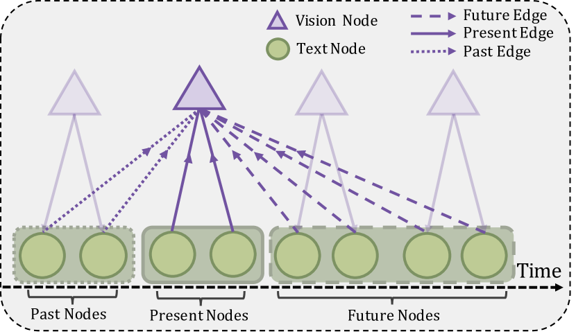
(a) Pseudo-Alignment example with less vision nodes

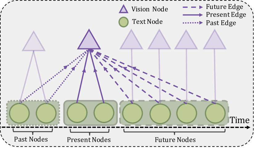
(b) Pseudo-Alignment example with more vision nodes

Figure 6: Examples of pseudo-align heuristic to coarsely define past, present and future relationships between two unaligned modalities. We try to spread and match the two modalities as much as uniformly possible (the top figure). When the shorter modality contains more and more nodes, we align as many nodes from the shorter sequence as possible with a minimum alignment window size of 2 to the longer sequence, and the rest nodes from the shorter sequence are aligned with window size of 1 (the bottom figure).

For node $v_{i}$ in $\pi_{i}$, in order to determine the “present" nodes $\mathbfcal{V}_{present}$ in a different modality, we draw an analogy from 1D convolution operation. We are given two sequences of different lengths, and we can treat the longer sequence as input and shorter sequence as output to a Conv1D operation. Our goal is to find a feasible stride and kernel size that aligns the input and output. The kernel size defines how many nodes from the longer sequence to be aligned as “present" to each node from the shorter sequence. The stride size defines how far away such alignments should spread in time. We do not consider any padding and have the following equation in Conv1D operation:

$$\frac{M-W}{S}+1=N$$ (8)

where $M$ and $N$ are the sequence lengths of the output and input to a Conv1D operator, respectively. $W$ is the kernel size and $S$ the stride size. From Eq. 8, we can further write the relationship between $W$ and $S$ as $W=M-(N-1)*S$. It is clear that the minimum stride size is 1 to a Conv1D operation, and the maximum is $\lfloor\frac{M}{N-1}\rfloor$ in order to keep $W$ positive. We take the average of the minimum and maximum possible values of $S$ as our stride size. In case that $N>\frac{M}{2}$, we set window size as 2 and stride as 2. We then find the maximal number of nodes from $N$ that can have kernel size of 2, and the rest of the nodes will have kernel size of 1. Eq. 9 shows our kernel size and stride size calculation and Figure. 6 illustrates our pseudo-alignment heuristic.

$$\begin{cases}S=\lceil\textbf{avg}(1,\lfloor\frac{M}{N-1}\rfloor)\rceil,&\hbox{\multirowsetup{if } $N\leq\frac{M}{2}$}\\ W=M-(N-1)*S&\\ S=2,W=2&\textbf{otherwise}\end{cases}$$ (9)

A.3 Model Efficiency

Figure 7: Convergence comparison between MTAG and MulT on validation set of unaligned CMU-MOSI dataset.

Hyperparameter	CMU-MOSI	IEMOCAP
Batch Size	64	64
Initial Learning Rate	1e-3	1e-3
Optimizer	Adam	Adam
Number of MTAG Layers	6	2
Number of Attention Heads	4	8
Node Embedding Dimension	64	64
Edge Pruning Keep Percentage	80$\%$	80%
Total Epochs	20	35

Table 6: Hyperparameter settings on CMU-MOSI and IEMOCAP benchmarks.

Number of Parameters.

We compare the parameter efficiency of our model against the SOTA model, the Multimodal Transformer (MulT) Tsai et al. (2019a). We first look at the total number of parameters used by the two models. Table 4 illustrates that our model uses 0.14 million parameters, only $6.3\%$ of those in MulT, which has 2.24 million parameters, and yet still achieves state-of-the-art performance. We attribute this result to the effective early fusion of multiple (more than 2) modalities using the MTAG component. In MulT, trimodal fusion happens at a very late stage of the architecture, since each cross-modal Transformer can only model bi-modal interactions. This late fusion regime requires earlier layers to preserve more original information, and thus resulting in a need for more model parameters.

Model \ Dataset	CMU-MOSI	IEMOCAP
MulT	$27.2_{\pm 2.33}$	$56.0_{\pm 4.59}$
MTAG (ours)	$\bf 24.4_{\pm 0.95}$	$\bf 44.4_{\pm 0.55}$

Table 7: Training time per epoch (in seconds) comparison. Run time is averaged over 5 training epochs, with the subscript denoting standard deviation. Both models use batch_size=32, num_layers=6 and are run on the same machine with a single GPU of Nvidia GTX 1080 Ti. Both benchmarks used are the unaligned version.

Convergence.

Figure 7 gives a comparison between the convergence speed of our model and MulT. Both models are trained with batch_size=32 and lr=1e-3, with the default (best) hyperparameters used for both models. We use the unalignd CMU-MOSI for this study. We observe MTAG converges much faster at epoch 12, comparing with MulT at epoch 17. In addition, we see that our validation MAE curve on the unaligned MOSI validation set goes consistently below MulT’s curve. This faster convergence performance could be explained by the small amount of parameters MTAG uses - MTAG has a much smaller parameter search space for the optimizer, resulting in faster training and earlier convergence.

Training time.

We also compare how fast our model runs against MulT. Specifically, under the same condition, we calculate the time it takes for each model to run training for 1 epoch. Table 7 shows the details. We can see that our model runs significantly faster than MulT on both benchmarks, which can be attributed to our light-weight model design (as shown in Table 8). Meanwhile, our edge pruning also reduces the number of computation by throwing away edges that are deemed less important by the model, thus improving the run-time of our model.

Overall Efficiency.

From the perspective of training time, number of parameters used, and convergence analysis, it is clear that our model is capable of achieving better results while using much smaller amount of computational resources than the previous state of the art.

Model	# Parameters
MulT (previous SOTA)	2,240,921
MTAG (ours)	142,363

Table 8: Number of model parameters comparison.

A.4 Hyperparameters

We elaborate on the technical details including hyperparameter settings in Table 6. We conduct a basic grid search to find good hyperparameters such as initial learning rate, number of MTAG layers etc. We use Adam as our optimizer and decays the learning rate by half whenever the validation loss plateaus. Notice that we are using a design that roughly yields a model with a similar structure as in previous works such as MulT. Nevertheless, we still manage to use far less number of parameters during optimization. We use one NVIDIA GTX 1080 Ti for training and evaluation. In addition, the model and hyperparameters we use for ablation study are the same as the ones used for the main experiment, both of which are conducted on CMU-MOSI.

A.5 Number of Parameters Comparison

For a fair comparison on number of parameters between MTAG and MulT, we use the same number of layers and attention heads for both models (i.e. 6 layers of MulT with 4 attention heads). A detailed comparison is shown in Table 8.

References

- Busso et al. (2008) Carlos Busso, Murtaza Bulut, Chi-Chun Lee, Abe Kazemzadeh, Emily Mower, Samuel Kim, Jeannette N Chang, Sungbok Lee, and Shrikanth S Narayanan. 2008. Iemocap: Interactive emotional dyadic motion capture database. Language resources and evaluation, 42(4):335.
- Degottex et al. (2014) Gilles Degottex, John Kane, Thomas Drugman, Tuomo Raitio, and Stefan Scherer. 2014. Covarep—a collaborative voice analysis repository for speech technologies. In 2014 ieee international conference on acoustics, speech and signal processing (icassp), pages 960–964. IEEE.
- Dumpala et al. (2019) Sri Harsha Dumpala, Imran Sheikh, Rupayan Chakraborty, and Sunil Kumar Kopparapu. 2019. Audio-visual fusion for sentiment classification using cross-modal autoencoder. In Proc. Neural Inf. Process. Syst.(NIPS), pages 1–4.
- Gori et al. (2005) Marco Gori, Gabriele Monfardini, and Franco Scarselli. 2005. A new model for learning in graph domains. In Proceedings. 2005 IEEE International Joint Conference on Neural Networks, 2005., volume 2, pages 729–734. IEEE.
- Graves et al. (2006) Alex Graves, Santiago Fernández, Faustino Gomez, and Jürgen Schmidhuber. 2006. Connectionist temporal classification: labelling unsegmented sequence data with recurrent neural networks. In Proceedings of the 23rd international conference on Machine learning, pages 369–376.
- Gu et al. (2018) Yue Gu, Kangning Yang, Shiyu Fu, Shuhong Chen, Xinyu Li, and Ivan Marsic. 2018. Multimodal affective analysis using hierarchical attention strategy with word-level alignment. In Proceedings of the 56th Annual Meeting of the Association for Computational Linguistics (Volume 1: Long Papers), pages 2225–2235, Melbourne, Australia. Association for Computational Linguistics.
- Hamilton et al. (2017) Will Hamilton, Zhitao Ying, and Jure Leskovec. 2017. Inductive representation learning on large graphs. In Advances in neural information processing systems, pages 1024–1034.
- iMotions (2017) iMotions. 2017. Facial expression analysis.
- Khademi (2020) Mahmoud Khademi. 2020. Multimodal neural graph memory networks for visual question answering. In Proceedings of the 58th Annual Meeting of the Association for Computational Linguistics, pages 7177–7188, Online. Association for Computational Linguistics.
- Khare et al. (2020) Aparna Khare, Srinivas Parthasarathy, and Shiva Sundaram. 2020. Multi-modal embeddings using multi-task learning for emotion recognition. Interspeech 2020.
- Kipf and Welling (2016) Thomas N Kipf and Max Welling. 2016. Semi-supervised classification with graph convolutional networks. arXiv preprint arXiv:1609.02907.
- Knyazev et al. (2019) Boris Knyazev, Graham W Taylor, and Mohamed Amer. 2019. Understanding attention and generalization in graph neural networks. In Advances in Neural Information Processing Systems, pages 4202–4212.
- Lazaridou et al. (2015) Angeliki Lazaridou, Nghia The Pham, and Marco Baroni. 2015. Combining language and vision with a multimodal skip-gram model. arXiv preprint arXiv:1501.02598.
- Lee et al. (2019) J. Lee, Inyeop Lee, and Jaewoo Kang. 2019. Self-attention graph pooling. In ICML.
- Liang et al. (2018) Paul Pu Liang, Ziyin Liu, Amir Zadeh, and Louis-Philippe Morency. 2018. Multimodal language analysis with recurrent multistage fusion. arXiv preprint arXiv:1808.03920.
- Ngiam et al. (2011) Jiquan Ngiam, Aditya Khosla, Mingyu Kim, Juhan Nam, Honglak Lee, and Andrew Y Ng. 2011. Multimodal deep learning. In ICML.
- Nicolicioiu et al. (2019) Andrei Nicolicioiu, Iulia Duta, and Marius Leordeanu. 2019. Recurrent space-time graph neural networks. In Advances in Neural Information Processing Systems, pages 12838–12850.
- Pennington et al. (2014) Jeffrey Pennington, Richard Socher, and Christopher D Manning. 2014. Glove: Global vectors for word representation. In Proceedings of the 2014 conference on empirical methods in natural language processing (EMNLP), pages 1532–1543.
- Pham et al. (2019) Hai Pham, Paul Pu Liang, Thomas Manzini, Louis-Philippe Morency, and Barnabás Póczos. 2019. Found in translation: Learning robust joint representations by cyclic translations between modalities. In Proceedings of the AAAI Conference on Artificial Intelligence, volume 33, pages 6892–6899.
- Poria et al. (2017) Soujanya Poria, Erik Cambria, Devamanyu Hazarika, Navonil Majumder, Amir Zadeh, and Louis-Philippe Morency. 2017. Context-dependent sentiment analysis in user-generated videos. In Proceedings of the 55th Annual Meeting of the Association for Computational Linguistics (Volume 1: Long Papers), pages 873–883, Vancouver, Canada. Association for Computational Linguistics.
- Scarselli et al. (2008) Franco Scarselli, Marco Gori, Ah Chung Tsoi, Markus Hagenbuchner, and Gabriele Monfardini. 2008. The graph neural network model. IEEE Transactions on Neural Networks, 20(1):61–80.
- Schlichtkrull et al. (2017) Michael Schlichtkrull, Thomas N Kipf, Peter Bloem, Rianne van den Berg, Ivan Titov, and Max Welling. 2017. Modeling relational data with graph convolutional networks. arXiv preprint arXiv:1703.06103.
- Shi et al. (2016) Chuan Shi, Yitong Li, Jiawei Zhang, Yizhou Sun, and S Yu Philip. 2016. A survey of heterogeneous information network analysis. IEEE Transactions on Knowledge and Data Engineering, 29(1):17–37.
- Siriwardhana et al. (2020) S. Siriwardhana, Andrew Reis, Rivindu Weerasekera, and Suranga Nanayakkara. 2020. Jointly fine-tuning "bert-like" self supervised models to improve multimodal speech emotion recognition. In INTERSPEECH.
- Tsai et al. (2019a) Yao-Hung Hubert Tsai, Shaojie Bai, Paul Pu Liang, J. Zico Kolter, Louis-Philippe Morency, and Ruslan Salakhutdinov. 2019a. Multimodal transformer for unaligned multimodal language sequences. In Proceedings of the 57th Annual Meeting of the Association for Computational Linguistics, pages 6558–6569, Florence, Italy. Association for Computational Linguistics.
- Tsai et al. (2019b) Yao-Hung Hubert Tsai, Paul Pu Liang, Amir Zadeh, Louis-Philippe Morency, and Ruslan Salakhutdinov. 2019b. Learning factorized multimodal representations. ICLR.
- Veličković et al. (2018) Petar Veličković, Guillem Cucurull, Arantxa Casanova, Adriana Romero, Pietro Liò, and Yoshua Bengio. 2018. Graph Attention Networks. International Conference on Learning Representations. Accepted as poster.
- Wang et al. (2019a) Xiao Wang, Houye Ji, Chuan Shi, Bai Wang, Yanfang Ye, Peng Cui, and Philip S Yu. 2019a. Heterogeneous Graph Attention Network. In The World Wide Web Conference on - WWW ’19, pages 2022–2032, San Francisco, CA, USA. ACM Press.
- Wang et al. (2019b) Yansen Wang, Ying Shen, Zhun Liu, Paul Pu Liang, Amir Zadeh, and Louis-Philippe Morency. 2019b. Words can shift: Dynamically adjusting word representations using nonverbal behaviors. In Proceedings of the AAAI Conference on Artificial Intelligence, volume 33, pages 7216–7223.
- Wei et al. (2019) Yinwei Wei, Xiang Wang, Liqiang Nie, Xiangnan He, Richang Hong, and Tat-Seng Chua. 2019. MMGCN: Multi-modal Graph Convolution Network for Personalized Recommendation of Micro-video. In Proceedings of the 27th ACM International Conference on Multimedia, pages 1437–1445, Nice France. ACM.
- Yang et al. (2020) Kaicheng Yang, Hua Xu, and Kai Gao. 2020. Cm-bert: Cross-modal bert for text-audio sentiment analysis. In Proceedings of the 28th ACM International Conference on Multimedia, MM ’20, page 521–528, New York, NY, USA. Association for Computing Machinery.
- Yin et al. (2020) Yongjing Yin, Fandong Meng, Jinsong Su, Chulun Zhou, Zhengyuan Yang, Jie Zhou, and Jiebo Luo. 2020. A novel graph-based multi-modal fusion encoder for neural machine translation. In Proceedings of the 58th Annual Meeting of the Association for Computational Linguistics, pages 3025–3035, Online. Association for Computational Linguistics.
- Zadeh et al. (2016) Amir Zadeh, Rowan Zellers, Eli Pincus, and Louis-Philippe Morency. 2016. Multimodal sentiment intensity analysis in videos: Facial gestures and verbal messages. IEEE Intelligent Systems, 31(6):82–88.
- Zheng et al. (2020) Chen Zheng, Quan Guo, and Parisa Kordjamshidi. 2020. Cross-modality relevance for reasoning on language and vision. ACL 2020.