The Cluster HEritage project with XMM-Newton:

The Cluster HEritage project with XMM-Newton - Mass Assembly and Thermodynamics at the Endpoint of structure formation (CHEX-MATE) is a three-mega-second Multi-Year Heritage Programme to obtain X-ray observations of a minimally-biased, signal-to-noise-limited sample of 118 galaxy clusters detected by Planck through the Sunyaev-Zeldovich effect. The programme, described in detail in this paper, aims to study the ultimate products of structure formation in time and mass. It is composed of a census of the most recent objects to have formed (Tier-1: $0.05<z<0.2$; $2\times 10^{14}$ M${}_{\odot}<M_{\rm 500}<9\times 10^{14}$ M_⊙), together with a sample of the highest mass objects in the Universe (Tier-2: $z<0.6$; $M_{\rm 500}>7.25\times 10^{14}$ M_⊙). The programme will yield an accurate vision of the statistical properties of the underlying population, measure how the gas properties are shaped by collapse into the dark matter halo, uncover the provenance of non-gravitational heating, and resolve the major uncertainties in mass determination that limit the use of clusters for cosmological parameter estimation. We will acquire X-ray exposures of uniform depth, designed to obtain individual mass measurements accurate to $15-20\%$ under the hydrostatic assumption. We present the project motivations, describe the programme definition, and detail the ongoing multi-wavelength observational (lensing, SZ, radio) and theoretical effort that is being deployed in support of the project.

1 Introduction

Clusters of galaxies provide valuable information on cosmology, from the physics driving galaxy and structure formation, to the nature of dark matter and dark energy (see e.g. Allen et al. 2011; Kravtsov & Borgani 2012). They are the nodes of the cosmic web, constantly growing through accretion of matter along filaments and via occasional mergers, and their matter content reflects that of the Universe ($\sim 85\%$ dark matter, $\sim 12\%$ X-ray emitting gas and $\sim 3\%$ galaxies). Clusters are therefore excellent laboratories for probing the physics of the gravitational collapse of dark matter and baryons, and for studying the non-gravitational physics that affects their baryonic component. As cluster growth and evolution depend on the underlying cosmology (through initial conditions, cosmic expansion rate, and dark matter properties), their number density as a function of mass and redshift, their spatial distribution, and their internal structure, are powerful cosmological probes.

Historically, optical and X–ray surveys have been the primary source of cluster catalogues. However, they can also be detected and studied via the Sunyaev-Zel’dovich effect (SZE; Sunyaev & Zeldovich 1972; Birkinshaw 1999; Carlstrom et al. 2002; Mroczkowski et al. 2019), the spectral distortion of the cosmic microwave background (CMB) generated through inverse Compton scattering of CMB photons by the hot electrons in the intra-cluster medium (ICM). The SZE brightness is independent of the distance to the object, and the total signal, $Y_{\rm SZ}$, is proportional to the thermal energy content of the ICM and is expected to be tightly correlated to the total mass (da Silva et al. 2004; Motl et al. 2005). SZE surveys such as those from the Atacama Cosmology Telescope (ACT; Marriage et al. 2011; Hasselfield et al. 2013; Hilton et al. 2018), the South Pole Telescope (SPT; Bleem et al. 2015, 2020) and Planck (Planck Collaboration VIII 2011; Planck Collaboration XXIX 2014; Planck Collaboration XXVII 2016) have provided cluster samples up to high $z$. These are thought to be as near as possible to being mass-selected, and as such are minimally-biased. The advent of these SZE-selected cluster catalogues, combined with new and archival X–ray information, has been transformational.

Indeed, X-ray follow-up of these new objects has raised new questions. The discovery that X-ray-selected and SZ-selected samples do not appear to have the same distribution of dynamical states (e.g. Planck Collaboration IX 2011; Rossetti et al. 2016; Andrade-Santos et al. 2017; Lovisari et al. 2017) has prompted examination of the relationship between the baryon signatures and the underlying cluster population. The possible tension between the value of the normalised matter density parameter, $\sigma_{8}$, obtained from cluster number counts, and that based on CMB measurements, has stimulated work on the absolute mass scale of clusters (see Pratt et al. 2019, for a review). With the advent of very high redshift ($z>1$) detections through the SZE, the issue of how to build a fully consistent picture of population evolution has also come to the fore.

In its 2017 Announcement of Opportunity, ESA offered the possibility to propose Multi-Year Heritage (MYH) programmes using the X-ray satellite XMM-Newton for the first time. This prompted a large response from the community, and the resulting oversubscription factor for the MYH proposal class was around ten. Two programmes were awarded MYH status, one of which was led by our collaboration (PIs: M. Arnaud, CEA Saclay; S. Ettori, INAF OAS Bologna). The project, now titled Cluster HEritage project with XMM-Newton - Mass Assembly and Thermodynamics at the Endpoint of structure formation (CHEX-MATE), aims to obtain complete and homogeneous X-ray exposures of 118 Planck SZE-selected galaxy clusters.

The sample comprises a minimally biased census both of the population of clusters at the most recent time ($0.05<z<0.2$), and of the most massive objects to have formed at $z<0.6$. It was designed to answer the following questions:

• What is the absolute cluster mass scale? What is the imprint of the formation process on the equilibrium state of clusters, and how does this impact our ability to weigh them through their baryon signature?

• What are the statistical properties of the cluster population? How does cluster detectability depend on baryon physics?

• Can we accurately measure how the properties of the cluster population change over time? What are the ultimate products of structure formation?

The X-ray observations started in Summer 2018 and would continue for three years. All the data are made public as soon as they are acquired. Planck SZE data are available for the full data set. Access to independent weak lensing (WL) mass estimates for a sizeable fraction of the sample was ensured through an object selection strategy that optimised coverage with existing high-quality optical multi-band imaging data from the Canada-France-Hawaii Telescope (CFHT), Subaru, and the Hubble Space Telescope (HST). Coverage was also optimised with the ongoing Canada-France Imaging Survey (CFIS) on the CFHT, and with the Euclid survey footprints.

This paper presents a detailed overview of the project, and acts as a reference for the collaboration and for the wider community. It is organised as follows. In Sect. 2, we present the motivating questions, scientific goals, and legacy value of such a project. In Sect. 3, we discuss the sample definition and observation strategy. Section 4 describes the supporting data essential to the project goals, and we present our summary and conclusions in Sect. 5. Throughout the paper we assume a flat $\Lambda$CDM cosmology with $\Omega_{m}=0.3$, $\Omega_{\Lambda}=0.7$ and $H_{0}=70$ km s^-1 Mpc^-1. The variables $M_{\Delta}$ and $R_{\Delta}$ are the total mass and radius corresponding to a total density contrast $\Delta\,\rho_{\rm c}(z)$, where $\rho_{\rm c}(z)$ is the critical density of the Universe at the cluster redshift; thus, for example, $M_{500}=(4\pi/3)\,500\,\rho_{\rm c}(z)\,R_{500}^{3}$. The quantity $Y_{\rm X}$ is the product of $M_{\rm g,500}$, the gas mass within $R_{500}$, and $T_{\rm X}$, the spectroscopic temperature measured in the $[0.15$–$0.75]\leavevmode\nobreak\ R_{500}$ aperture. The SZ flux is characterised by $Y_{\Delta}$, where $Y_{\Delta}\,D_{\rm A}^{2}$ is the spherically integrated Compton parameter within $R_{\Delta}$, and $D_{\rm A}$ is the angular-diameter distance to the cluster.

2 CHEX-MATE description

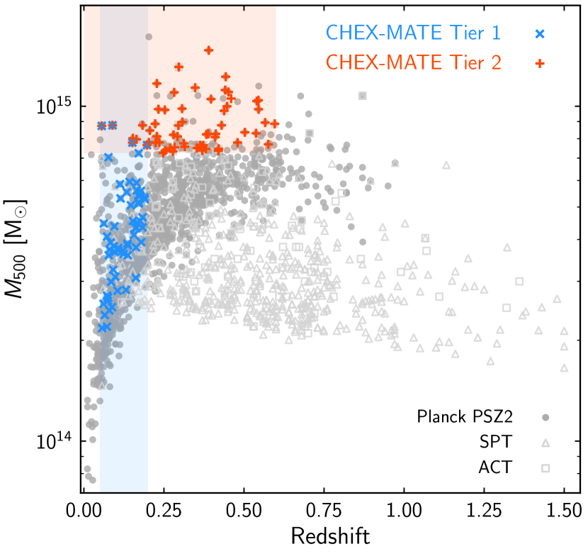
Figure 1: Distribution in the $M_{\rm 500}-z$ plane of confirmed clusters from major SZE surveys, available at the time of proposal submission (October 2017). Filled circles: Planck  clusters (Planck Collaboration VIII 2011; Planck Collaboration XXIX 2014; Planck Collaboration XXVII 2016); triangles: SPT (Bleem et al. 2015); squares: ACT (Hasselfield et al. 2013). Masses for Planck clusters are derived iteratively from the $Y_{\rm SZ}$–$M_{\rm 500}$ relation calibrated using masses from XMM-Newton; these were not corrected for any HE bias (see text for details). The figure includes both masses published in the Planck catalogue, and new masses computed using new redshift information. The shaded boxes indicate the Tier-1 and Tier-2 redshift ranges in blue and orange, respectively. The sample is drawn from the Planck PSZ2 sample, selecting clusters detected at high signal-to-noise ratio (S/N$>6.5$) with the MMF3 algorithm, and in the cleanest part of the sky. We also excluded clusters in the sky region with poor XMM-Newton visibility. Additional redshift, sky area, mass criteria, are applied to define the Tier-1 ($0.05<z<0.2;\ {\rm Dec}>0$) and Tier-2 ($z<0.6$, $M_{500}>7.25\times 10^{14}{\rm M_{\odot}}$) samples. Remaining clusters in the shaded part of the $M_{\rm 500}-z$ plane are at lower S/N, or lie outside the sky regions under consideration. A full description of the sample strategy is given in Sec. 3.1 and is further illustrated in Appendix A.

2.1 Motivating questions

Inspired by the new results obtained from the objects found in SZE-selected cluster surveys, and from their subsequent multi-wavelength follow-up, the project is built around a series of questions.

2.1.1 What is the absolute cluster mass scale?

Theory predicts the number of clusters as a function of their redshift and mass. Surveys detect clusters through their observable baryon signature such as their X-ray or SZE signal, or the optical richness. To obtain cosmological constraints from the cluster population, this signal must then be linked to the underlying mass; in other words, one must know the relation between the observable and the mass, and the scatter about this relation. One must also understand the probability that a cluster of a given mass is detected with a given value of the survey observable; the resulting selection function is a key element in the cosmological analysis of the cluster population.

In the first Planck SZE cluster cosmology analysis, the SZE-mass scaling relation was derived from X‐ray observations and numerical simulations. They combined the $M_{500}$–-$Y_{X}$ relation obtained from a sample of relaxed clusters with masses derived from the hydrostatic equilibrium (HE) equation Arnaud et al. (2010), and the $Y_{\rm X}$–-$Y_{\rm SZ}$ relation calibrated on a subset of clusters from the cosmology sample (Planck Collaboration XX 2014, Appendix A). They introduced a mass bias parameter, $b$, to account for differences between the X-ray mass estimates and the true cluster halo mass: $M_{\Delta}=(1-b)\,M_{\Delta,{\rm true}}$. The factor $b$ encompasses all unknowns with regard to the relationship between the X-ray mass and the true mass, such as can arise from observational effects such as instrumental calibration, or from cluster physics such as departure from HE or temperature structure in the ICM.

The main result from the Planck SZE cluster count analysis was that, with a fiducial $(1-b)=0.8$, derived from numerical simulations, the $\sigma_{8}$ and $\Omega_{\rm m}$ values obtained from SZE cluster abundances were inconsistent at the $\sim 2\sigma$ level with the values derived from the Planck CMB cosmology (Planck Collaboration XXIV 2016; Planck Collaboration XIII 2016). For the 2015 analysis, a value of $(1-b)=0.58\pm 0.04$ would be needed reconcile cluster counts and CMB measurements, implying a much larger HE bias than expected from numerical simulations. The value needed to reconcile cluster counts and CMB reduces to $(1-b)=0.62\pm 0.03$ in the 2018 Planck CMB analysis. This is still considerably larger than expectations. Inclusion of additional constraints from the thermal SZ power spectrum similarly implies $(1-b)\lesssim 0.67$ (Salvati et al. 2018).

Prompted by these results, the cluster mass determination, and its relation to the observable, have become issues of great debate in the community (see e.g. the review of Pratt et al. 2019). Important new constraints on the value of $(1-b)$ have come from WL mass measurements of sizeable samples with good control of systematic effects (e.g. the Cluster Lensing and Supernova Survey with Hubble - CLASH, Postman et al. 2012; the Canadian Cluster Cosmology Project - CCCP, Hoekstra et al. 2015; Herbonnet et al. 2020; Weighing the Giants - WtG, von der Linden et al. 2014; the Local Cluster Substructure Survey - LoCuSS, Smith et al. 2016; PSZ2LenS, Sereno et al. 2017). However, a consensus has not been reached, with, for example, WtG finding $(1-b)=0.69\pm 0.07$, marginally reconciling CMB and cluster constraints (Planck Collaboration XIII 2016) and implying a large HE bias, but LoCuSS measuring $(1-b)=0.95\pm 0.04$, indicating a low HE bias. An alternative mass measurement from lensing of the CMB itself by clusters initially suggested no significant bias (e.g. Melin & Bartlett 2015); however, recent re-analysis by Zubeldia & Challinor (2019), including the mass bias factor directly in the cosmological analysis, finds $(1-b)=0.71\pm 0.10$.

The theoretical picture is also uncertain. A significant upward revision of the total mass would imply that cluster baryon fractions were significantly lower than the universal value, at odds with expectations from numerical simulations (e.g. Planelles et al. 2017; Ansarifard et al. 2020). Similarly, while simulations predict some turbulence and non-thermal pressure support from gas motions generated by the hierarchical assembly process, they do not indicate that clusters are strongly out of equilibrium on average (e.g. Biffi et al. 2016; Ansarifard et al. 2020; Angelinelli et al. 2020). Recent observational constraints also suggest that this is not the case, at least in relaxed nearby massive systems (Eckert et al. 2019).

Larger samples of high-quality data are needed to reduce the statistical uncertainties in the absolute mass calibration, and to fully characterise any residual intrinsic scatter. This can best be achieved through a sample selection strategy that reflects as closely as possible the underlying population.

2.1.2 What is the ‘true’ underlying cluster population?

Current surveys detect clusters through their baryon signature. The SZE signal, proportional to the integral of the gas pressure along the line of sight, has been shown to behave well, with a weak dependence on dynamical state and on poorly understood non-gravitational physics (da Silva et al. 2004; Planelles et al. 2017). A comparison of Planck SZE selected clusters with X-ray selected clusters indicated that the former are on average less relaxed (using gas morphological indicators or BCG-centre offset), and contain a lower fraction of over-dense, cool core systems (Planck Collaboration IX 2011; Rossetti et al. 2016, 2017; Andrade-Santos et al. 2017; Lovisari et al. 2017, see also Zenteno et al. 2020 for a different view).

This may reflect the tendency of X-ray surveys to preferentially detect clusters with a centrally-peaked morphology, which are more luminous at a given mass, and on average more relaxed (e.g. Pesce et al. 1990; Pacaud et al. 2007; Eckert et al. 2011). However, it is currently unclear if this selection effect is sufficient to explain the difference (e.g. Rossetti et al. 2017). This also raises concerns about how representative the X-ray selected samples, used to define our current understanding of cluster physics and to calibrate numerical simulations, have been. Examples, frequently used in the literature, include the REXCESS sample of 33 clusters with deep XMM-Newton data (Böhringer et al. 2007; Pratt et al. 2009, 2010; Arnaud et al. 2010), or the sample of relaxed clusters with deep Chandra observations studied by Vikhlinin et al. (2006).

We expect a sample selected through its SZE signal to be more representative of the underlying population, and as such the least biased that it is currently possible to obtain. The ensemble properties of such a sample will yield critical insights into the gas thermodynamic properties and their relation to the cluster mass, and into how variations in gas properties feed into the survey selection function.

2.1.3 Can we measure how the properties of the cluster population change over time?

Chandra follow-up of clusters detected by the SPT between redshift $0.3$ and $1.9$ has indicated that the average ICM properties outside the core are remarkably self-similar, with no measurable evolution of morphological dynamical indicators (McDonald et al. 2014, 2017; Nurgaliev et al. 2017). These observations also suggested that cool cores are formed early and are very stable to further dynamical evolution. However, as the SPT survey is highly incomplete below $z=0.3$, this study relies on an X-ray-selected sample to provide the low-$z$ anchor. Due to the selection effects outlined above, we do not yet have a fully consistent picture of population evolution.

The redshift independence of the SZE has led to the discovery of many hundreds of high-redshift systems, with which studies of how the properties of the cluster population change with time can be undertaken. However, such studies need a well-characterised low-redshift anchor obtained with the same selection method.

2.2 Immediate scientific goals

The questions discussed above led to the definition of CHEX-MATE, a sample of 118 clusters detected by Planck at high signal-to-noise (S/N$>6.5$) through their SZE signal. Figure 1 shows the sample in the $z-M$ plane. It is composed of:

• Tier-1: a census of the population of clusters at the most recent time ($0.05<z<0.2$, with $2\times 10^{14}$ M${}_{\odot}<M_{\rm 500}<9\times 10^{14}$ M_⊙);

• Tier-2: the most massive systems to have formed thus far in the history of the Universe ($z<0.6$, with $M_{\rm 500}>7.25\times 10^{14}$ M_⊙).

The 61 clusters in Tier-1 provide an unbiased view of the population at the present time, and serve as the fundamental anchor of any study that seeks to assess how the population changes over cosmic time. The 61 objects in Tier-2 comprise the most massive clusters, the ultimate manifestation of hierarchical structure formation, which the local volume is too limited to contain. Four systems are common to both Tiers. In the following, we describe the detailed scientific goals of the project.

2.2.1 The dynamical collapse of the ICM

The extent to which the gas is in equilibrium in the dark matter potential, as a function of mass and radius, is a key issue for the understanding of the mass scale. This is linked to the presence of turbulence in the ICM, non-thermal electrons (detectable in radio emission), shocks, bulk motion, and sub-clustering at all scales. Objective morphological indicators (e.g. centroid shifts, power ratios etc) will be provided by the X–ray imaging (Lovisari et al. 2017). An exciting new development is the use of surface brightness fluctuations to constrain the turbulence spectrum (Gaspari & Churazov 2013; Zhuravleva et al. 2014; Hofmann et al. 2016; Eckert et al. 2017). Combining SZE and X-ray imagery will allow us to constrain gas clumpiness and the thermodynamical properties in the outskirts, as addressed in the X-COP project (see e.g. Eckert et al. 2017; Ghirardini et al. 2019; Eckert et al. 2019; Ettori et al. 2019). We will measure various key ICM parameters, their dependence on mass, and study outliers in detail. These results will provide key information for our investigation of mass biases, as discussed below. We will correlate with radio surveys to link the dynamical indicators to the presence and extent of non-thermal energy contained in radio halos and relics.

Furthermore, simulations show that the most massive clusters always form at the crossroads of the hottest filaments. Objects with $M\sim 10^{15}\leavevmode\nobreak\ \rm M_{\odot}$ have an $\geq 80\%$ probability of being connected by a filament of dark and luminous matter to a neighbouring cluster at a distance of $<15\ {\rm Mpc}/h$ (Colberg et al. 2005). The field of view (FoV) of XMM-Newton allows the study of the large-scale environment of massive clusters, since a single pointing is sufficient to map the entire azimuth above $R_{200}$ in most of the massive (Tier-2) objects. In particular, in more than 60% of the Tier-2 objects, the XMM-Newton FoV subtends a region up to 2$R_{200}$. These systems are the ideal targets for a robust detection of the large-scale cosmic web (e.g. Haines et al. 2018). The possibility of studying gas compression and dynamical activity between clusters in an early merger stage has recently been raised by several radio observations (e.g. Akamatsu et al. 2017; Govoni et al. 2019; Botteon et al. 2020) and in numerical simulations (e.g. Vazza et al. 2019). Detecting and studying the rare merger configurations that may lead to the formation of cluster-cluster bridges will be an additional challenge for CHEX-MATE.

2.2.2 The cluster mass scale

We will measure total integrated mass profiles (out to at least $R_{500}$) for all objects using the equations derived from the HE assumption (e.g. Pratt & Arnaud 2002; Ettori et al. 2013). The total HE mass will be compared to mass proxies such as the SZE signal $Y_{\rm SZ}$, the X-ray luminosity $L_{\rm X}$ or $Y_{\rm X}$ (the product of ICM mass and temperature). Most importantly, WL data are already available for a significant fraction of the sample, especially at high mass (see Fig. 2). Section 4.1 details the currently available lensing data and details the strategy we have deployed to obtain complete WL follow-up. Ultimately, follow-up will also be available with Euclid.

Comparison of these mass estimates (weak lensing mass M_WL, hydrostatic mass M_HE) and various mass proxies can be undertaken, measuring the best fitting scaling laws and scatter, and the covariance between quantities. Correlation with dynamical indicators and investigation of trends with mass can also be performed. This will be the first time that such an investigation of cluster masses will be performed systematically and self-consistently on a well defined and minimally-biased sample, covering the full mass range. Many comparisons based on reference samples (e.g. the Planck calibration samples, LoCuSS, CCCP, WtG) yield only a partial overview of the inter-dependence of the parameters (e.g. $M_{\rm WL}$–$M_{\rm HE}$ or $M_{\rm WL}$–$Y_{\rm SZ}$), as they are statistically incomplete due to limited coverage, or were compiled based on criteria such as archival availability.

All mass estimates are subject to inherent bias (see e.g. the review by Pratt et al. 2019 and references therein). The HE bias is well known to affect X-ray observations, but lensing is also subject to biases due to line-of-sight effects. While the lensing mass is expected to be the least biased on average, it is of lower statistical quality on an individual cluster basis (e.g.  Meneghetti et al. 2010; Hamana et al. 2012). Our goal is to build a consistent understanding of the various biases and to define the best strategy to obtain the most accurate mass estimate in various surveys.

2.2.3 The interplay between gravitational and non-gravitational processes

The densest core regions, where the interplay between cooling and central AGN feedback is strongest, provide key diagnostics on the impact of non-gravitational processes on the ICM (e.g. Cavagnolo et al. 2009; Pratt et al. 2010). If cool cores are less prominent than previously thought from X-ray selected samples, we may have to fundamentally revise our vision of cooling and galaxy feedback at cluster scales.

With this sample, the true distribution of cool core strength (see e.g. Hudson et al. 2010) can be reassessed, as can the impact of feedback on the thermodynamical properties of the ICM as a function of radius, mass, and, at the high mass end, redshift. We can definitively establish the relation between core properties and the bulk, including dynamical state (e.g. Are cool cores essentially found in relaxed systems? To what extent are they destroyed by mergers?), thereby providing a testbed for predictions from numerical simulations (see e.g. Barnes et al. 2018).

As shown by a diverse range of studies, linking AGN feeding and feedback processes over nine orders of magnitude is vital to advancing our understanding of clusters and diffuse hot halos (see e.g. McDonald et al. 2018, Gaspari et al. 2020 for reviews). We can establish the new population-level baseline to understand the interplay between gravitational heating, cooling and AGN feedback. Covering the full range of masses probed by Planck, the sample includes both the highest mass systems dominated by gravitational heating, and lower mass systems that are progressively more affected by non-gravitational input. The radial coverage, from the core to at least $R_{500}$, is equally important for sampling the relative impact of the different energetic processes, and for obtaining the widest possible view of the gas morphology.

The measurement of metal abundances in the ICM is a powerful probe of the nature of galaxy feedback processes (see Mernier et al. 2018, Biffi et al. 2018, and references therein). The abundances yield information both on the various types of supernovae (core-collapse and SNIa) producing the metals throughout the cluster lifetime (reaching back to the proto-cluster phase), and on the AGN feedback mechanisms that spread the metals throughout the ICM. Although not tailored to the measurement of metal abundances out to $R_{500}$, our observations will enable measurement of the total amount of iron out to a significant fraction of $R_{500}$. We can test the uniformity of the metal enrichment in massive clusters as a function of redshift with Tier-2, and as a function of mass with Tier-1. By comparing with stellar masses, we will address the long-standing issue of whether the amount of iron in the ICM is in excess of what can be produced in the stars (e.g. Arnaud et al. 1992; Ghizzardi et al. 2020); and in particular with Tier-1, address the relation of the iron mass, ICM mass and stellar mass, to the total mass (e.g. Bregman et al. 2010; Renzini & Andreon 2014).

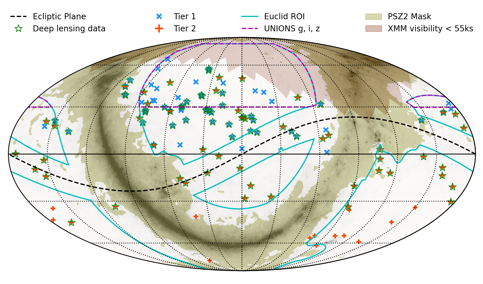
Figure 2: Sky distribution of Tier-1 (green) and Tier-2 (red) clusters detected in the Planck ‘cosmological’ mask, outside the dusty galactic plane (green shaded area), and outside the region of low XMM-Newton visibility (red shaded area). A further cut in declination is applied for Tier-1. The synergy in sky coverage between our SZE selected sample and the UNIONS/CFIS/Euclid lensing surveys is clear. In total, 107 targets fall in the footprint of the Euclid Region of Interest survey (cyan) and 33 in the UNIONS/CFIS survey footprint (pink). Clusters with existing or ongoing deep WL mass measurements are marked by stars (see Sect. 4.1 for details).

2.2.4 A local anchor for tracking population changes

Our project will yield the ultimate baseline for the statistical properties of nearby clusters and of the most massive clusters to have formed in $5.8$ Gyr look back time. It is based on a sample defined to be as unbiased as possible for detection based on baryon observables. We emphasise that the X-ray and lensing properties that we intend to measure will be independent of the detection signal, minimising the need for Eddington bias correction (although covariances between quantities will need to be taken into account). The major outputs of our project will include scaling laws, structural properties, and quantitative dynamical indicators, including dispersion and covariance between parameters. Tier-1 has three times more clusters than REXCESS, permitting a major step forward on the precision not only of the main trends, but also of the dispersion around them. The full sample size and mass coverage will allow the dispersion to be explored as a function of mass, and, at high mass, also as a function of redshift. Crucially, this work will be underpinned by the best possible control of systematics on cluster masses due to our self-consistent study of the mass scale and related biases. Our work will provide a state-of-the-art reference with which to anchor our view of how the population changes with time from ongoing Chandra and XMM-Newton follow-up of high-$z$ SZE clusters, and with which to calibrate the baryon physics in numerical simulations that are used to interpret surveys (e.g. as undertaken in the BAHAMAS project by McCarthy et al. 2017; see also Rasia et al. 2015 and the discussion in Sect. 4.5).

The project is of substantial value for next-generation X-ray and SZE surveys. Our sample corresponds to the descendants of the high–$z$ objects that will be detected by upcoming SZE surveys such as SPT-3G, which will probe lower masses than currently possible, and as such represents the culmination of the cluster evolutionary track. The project will also provide key input for the interpretation of eROSITA, the ongoing All-sky X-ray survey. The X-ray luminosity depends on the square of the gas density and is dominated by the core properties, which presents a large scatter and a strong dependence on thermodynamical state and the effect of non-gravitational processes. X–ray cluster detectability further depends on morphology, which is closely linked to the dynamical state (see Fig. 2 in Arnaud 2017). We can investigate the X-ray luminosity–mass relation and its scatter, together with its relation to the distribution of morphologies in the population, enabling us to understand these selection effects. Combined with improved measurements of cluster evolution, our work will provide the basis for robust modelling of the selection for any X-ray survey.

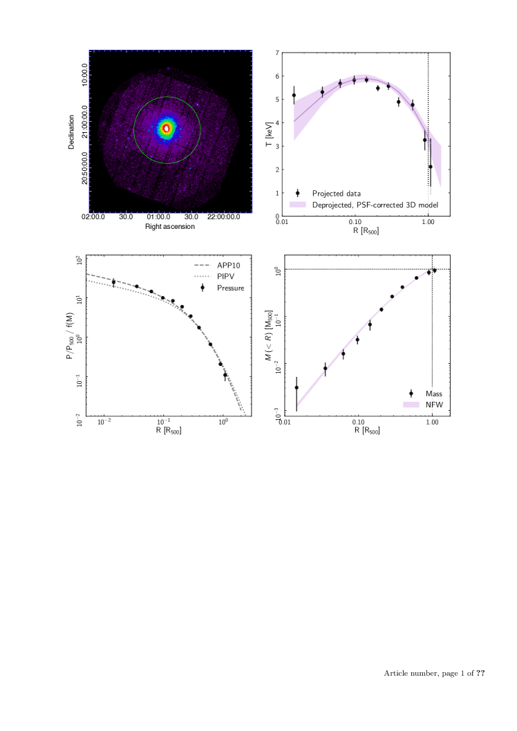
Figure 3: Example XMM-Newton image and radial profiles of the newly-observed cluster PSZ2  G$077.90-26.63$, detected at an S/N$\sim 178$ in the $[0.3-2]$ keV band in the $[0.15-1]\,R_{500}$ region. Top left: [0.3-2.0] keV image, with green circle indicating $R_{500}$. Top right: Raw temperature profile (black points) with best-fitting deconvolved, deprojected 3D model and corresponding $1\sigma$ uncertainties (envelope). Bottom left: Scaled pressure profile compared to the universal pressure profile of Arnaud et al. (2010, APP10) and the mean stacked profile of Planck Collaboration Int. V (2013, PIPV). $f(M)$ is a (small) correction for the mass dependence in the pressure profile shape (see Arnaud et al. 2010). Bottom right: Scaled hydrostatic integrated mass profile compared to the best-fitting NFW model with concentration $c_{500}=2.6^{+0.3}_{-0.2}$.

Category	Number of	Count rate (ct/s)			XMM time (ksec)
	clusters	min	med	max	Clean	Required
Observed & $R_{500}<15^{\prime}$	68	$0.8$	$2.9$	$24.0$	1850.9	782.9
Observed & $R_{500}>15^{\prime}$	3	$18.2$	$23.3$	$53.1$	420.7	0
New & $R_{500}<15^{\prime}$	47	$0.6$	$2.9$	$7.9$	0	1029.0

Table 1: Required exposures. In each category, the count rates (minimum, median and maximum), the cleaned XMM-Newton PN archived time, and the requested exposure time (with no overheads), are given. None of the three targets with $R_{500}>15^{\prime}$ require new exposures.

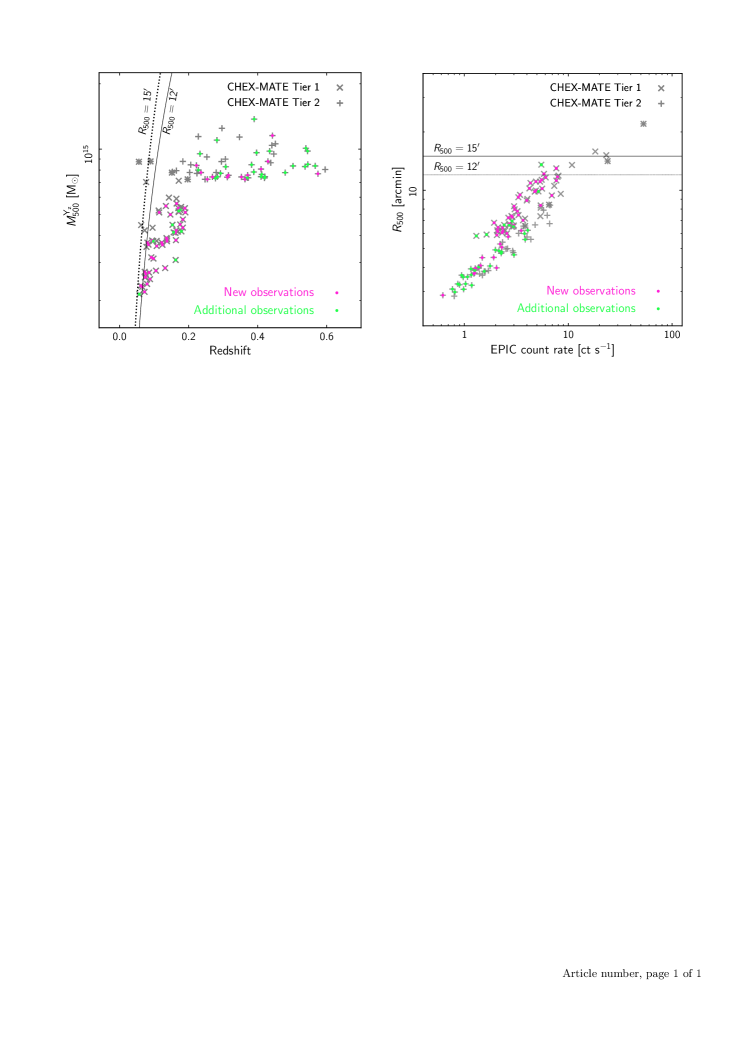
Figure 4: Left: Distribution of the required XMM-Newton observations in the $z$–$M$ plane. Right: Distribution in the size–count rate plane.

Ultimately, one would like a method to detect clusters based on their most fundamental property: the total mass. Our project will not be able to exclude the existence of baryon-poor clusters that are simply not detected in X–ray or SZE surveys. Even if we derive the gas properties from X-ray observations, independent of the original SZE detection, there is a residual, intrinsic, covariance with the SZE signal, through the total gas content. Detection of clusters based on their lensing signal, i.e. directly on projected mass, has started to become routinely possible with surveys such as the Hyper SupremeCam Survey (HSC; Miyazaki et al. 2018). The Euclid satellite (and the Rubin Observatory) will for the first time allow the detection of sizeable samples of clusters, including the rarest most massive objects, due to their unprecedented sky coverage. Our project has particular synergy with Euclid, the sensitivity of which should allow blind detection of objects in the redshift and mass range covered by our sample (Fig. 2). Comparison of SZE and shear-selected samples will be critical to assessing residual selection effects, if any. It will also be possible to extract high-quality individual and/or stacked shear profiles from Euclid data, as discussed in more detail in Sect. 4.1. The (nearly) all-sky coverage of the Tier-2 sample at high mass will provide the best targets for future strong lensing studies. As the most powerful gravitational telescope in the Universe, they will be high-priority targets for the James Webb Space Telescope (JWST). In the longer term, our sample will provide the targets of reference for dedicated Athena pointings for deep exploration of ICM physics both in representative (Tier-1) and extreme (Tier-2) clusters.

3 Observing strategy

3.1 Sample definition

The sample is extracted from the Planck PSZ2 catalogue (Planck Collaboration XXVII 2016), including only sources detected in the cosmological mask, which is the cleanest part of the sky (Planck Collaboration XXIV 2016). We then excluded the sky region with poor XMM-Newton visibility (median visibility less than $55$  ksec per orbit), which is located in the North (see Fig. 2). We applied a further cut imposing the signal-to-noise ratio (S/N) measured by the MMF3 detection method (Melin et al. 2006) to be larger than $6.5$, allowing us to have a well-controlled analytical selection function.

This parent sample includes 329 sources, all validated as clusters with $z$ estimates, except for two objects, PSZ2 G237.41-21.34 and PSZ2 G293.01-65.78. It is a sub-sample of the cosmological sample analysed by Planck Collaboration XXIV (2016), but with a slightly higher S/N cut and a more restricted sky region due to the addition of the XMM-Newton visibility criteria. Tier-1 consists of the 61 local $0.05<z<0.2$ clusters in the Northern sky (${\rm Dec}>0$). In this region, the validation is now $100\%$ complete (Barrena et al. 2018; Aguado-Barahona et al. 2019, Dahle et al. in prep.), and the overlap with the CFIS survey (Ibata et al. 2017) is maximised. The Tier-1 sample has a median mass of $M_{\rm 500}=4.1\times 10^{14}\,{\rm M_{\odot}}$, as compared to $5.9\times 10^{14}\,{\rm M_{\odot}}$ for the Planck Early SZ (ESZ) sample (Planck Collaboration VIII 2011). Tier-2 includes all 61 clusters above $M_{500}>7.25\times 10^{14}\,{\rm M_{\odot}}$, as estimated from the MMF3 SZE signal, at $z<0.6$. For this sample of the rarest massive clusters, we had to consider the full parent sample, which at the time of proposal submission was not fully validated. However, the SZE flux of the two sources with missing validation information is such that they would not enter into the Tier-2 selection even if they lie at redshift $z<0.6$. Four clusters are common to Tiers-1 and 2, for a total of 118 clusters, 47 of which have never been observed with XMM-Newton.

The sample distribution in the $z$-$M_{\rm 500}$ plane is shown in Fig. 1, and its distribution on the sky is shown in Fig. 2. The details of the selection process in the $z$–$M_{500}$ plane is further illustrated in Fig 11 in Appendix A.

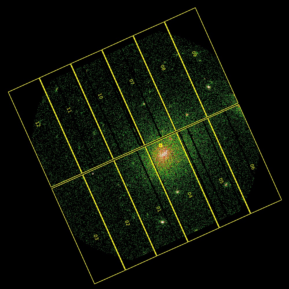
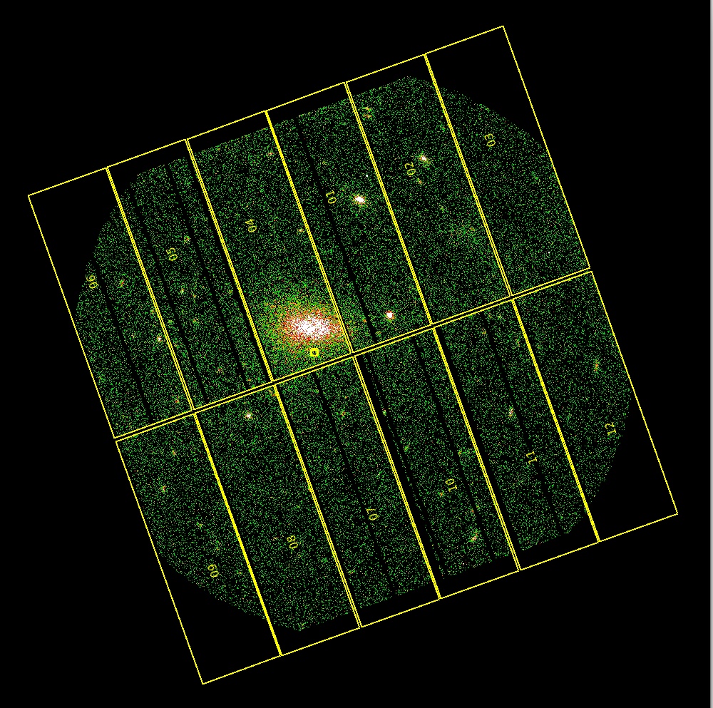
Figure 5: Illustration of the boresight strategy. Left panel: PN image of PSZ2 G057.78+52.32, at $z=0.0654$, Right panel: PN image PSZ2 G066.41+27.03, at $z=0.575$. The yellow grid shows the layout of the PN camera with the nominal boresight marked with a small box. Depending on the roll angle, the observation boresight is moved $2^{\prime}$ along pn CCD 4. This avoids the cluster centre region being affected by gaps between CCD chips.

3.2 X-ray observation setting

3.2.1 Exposure time

The key observation driver is to obtain temperature profiles up to $R_{500}$. We used the mass obtained from the SZE mass proxy, $M_{500}^{\rm YSZ}$, estimated from the $Y_{\rm SZ}$ signal (Planck Collaboration XXIX 2014) to obtain the corresponding radii. From our analysis of Planck clusters (Planck Collaboration XI 2011), we find a tight correlation between $M_{\rm 500}$ and the core excised luminosity in the soft $[0.5$–$2]$ keV band when scaled according to purely self-similar evolution, in agreement with the REXCESS X-ray sample. The expected soft band count rates in the core excised region ($[0.15$–$1]R_{500}$) are therefore expected to be particularly robust. The conversion between the luminosity and XMM-Newton European Photon Imaging Camera (EPIC; PN $+$ MOS) counts takes into account the Galactic column density ($N_{\rm H}$) value and redshift. We checked that the predicted count rates are consistent with those observed for the ESZ-XMM archival sample we have already analysed (see e.g. Planck Collaboration XI 2011; Lovisari et al. 2017) . If we define the count rate from the source, the background, and the total as $C_{\rm s}=CR_{\rm s}\times t_{\rm exp}$, $C_{\rm b}=CR_{\rm b}\times t_{\rm exp}$, and $C_{\rm t}=(CR_{\rm s}+CR_{\rm b})\times t_{\rm exp}$, respectively, then the S/N within the core excised region is, assuming a Gaussian error propagated in quadrature,

$${\rm S/N}=\frac{C_{\rm s}}{\sqrt{C_{\rm t}+C_{\rm b}}}=\frac{CR_{\rm s}\sqrt{t_{\rm exp}}}{\sqrt{CR_{\rm s}+2\times CR_{\rm bkg}}}.$$ (1)

Here, we define the core excised region as $\pi\,(1.-0.15^{2})\,R_{500}^{2}$, and adopt $CR_{\rm bkg}\sim 1.3\times 10^{-2}\,{\rm cts\ s^{-1}\ arcmin^{-2}}$ in the [0.3-2]  keV band.

We set the exposure time, $t_{\rm exp}$, to reach an S/N$=150$. From our study of ESZ-XMM data, this is sufficient to map the temperature profile in $8+$ annuli at least up to $R_{500}$ with a precision of $\pm 15\%$ in the $[0.8$–$1.2]R_{500}$ annulus, and to reach an uncertainty of $\pm 2\%$ (statistical uncertainty) on the mass derived from the $Y_{\rm X}$ mass proxy, $M_{\rm 500}^{YX}$, and to derive the HE mass measurements at $R_{500}$ to the $\sim 15$–$20\%$ precision level. The precision is illustrated in Fig 3, where we show an analysis of the representative observation of PSZ2 G$077.90-26.63$, which reaches the required S/N.

With regard to archival XMM-Newton observations, we processed all archival observations (including offset pointings) of Tier-1 and Tier-2 ($71$ clusters in total) to estimate the clean (soft proton flare-free) time of the PN camera. This was subtracted from the requested time. Thirty-three clusters needed re-observations. They are marked in Fig. 4 with green points, together with the 47 clusters that have never been never observed with XMM-Newton before (pink points).

The $R_{500}$ size of three clusters is larger than the XMM-Newton $15^{\prime}$ field of view (see Fig. 4 and Table 1); for these three objects, offset pointings are available in the archive to enable detection of the ICM to $R_{500}$. For four clusters with $12^{\prime}<R_{500}<15^{\prime}$ and without offset observations in the XMM-Newton  archive, we required one extra $15$  ksec pointing for precise background measurements.

The final total project observing time is summarised in Table 1. The required time was increased by $40\%$ to account for time loss owing to soft proton flares, and a minimum exposure time of 15 ksec was set to enable efficient use of XMM-Newton (in view of observation overheads and slew time). The final list of CHEX-MATE target observations, including archival observations, is presented in Tables 3.2.1, 3.2.1, and 3.2.1. These tables list all target properties that were used in the selection and exposure time estimation.

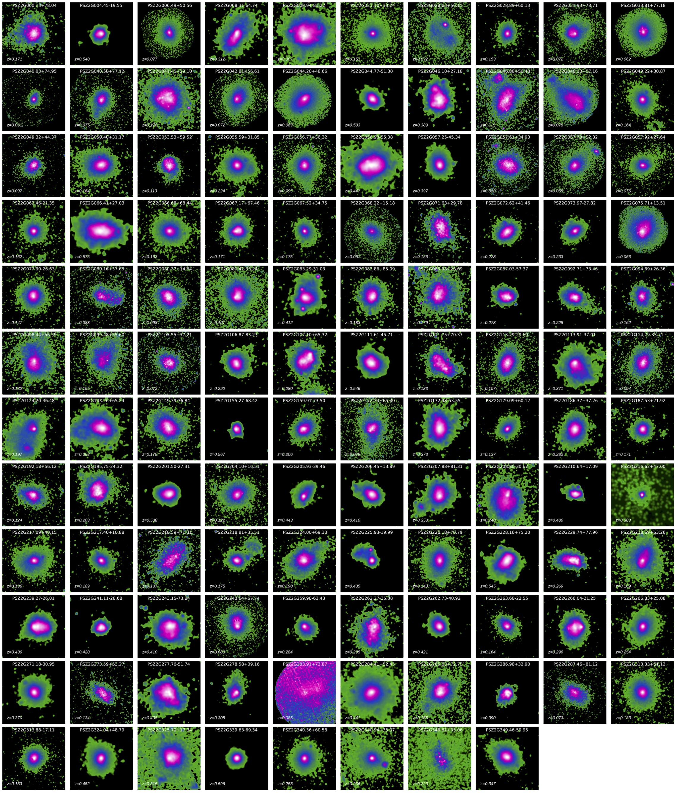
Figure 6: XMM-Newton image gallery of the 118 targets. The images cover an area of 2.4 $R_{500}\times$ 2.4 $R_{500}$. After the main point sources have been masked and their emission has been replaced with an average contribution from the nearby environment, they are background subtracted, exposure corrected and smoothed with a Gaussian with $\sigma$ = 7.5 arcsec. Low-quality images correspond to objects for which the exposure time will be completed in the final year of observations.

Name	RA	Dec	obsID	$t_{\rm clean}$
	h:m:s	d:m:s		ksec
PSZ2 G113.91-37.01	00:19:39	+25:17:27	21059	9.8
PSZ2 G217.40+10.88	07:38:19	+01:02:07	21060	9.6
PSZ2 G083.86+85.09	13:05:51	+30:54:17	21061	9.8
PSZ2 G149.39-36.84	02:21:34	+21:21:57	21062	9.9
PSZ2 G062.46-21.35	21:04:54	+14:01:40	21063	9.9
PSZ2 G218.59+71.31	11:29:55	+23:48:14	21064	9.8
PSZ2 G028.63+50.15	15:40:09	+17:52:41	21065	9.8
PSZ2 G080.16+57.65	15:01:08	+47:16:35	21066	10.3

Table 2: List of the eight objects with a dedicated Chandra snapshot. RA and Dec refer to the Chandra pointing coordinates; obsID identifies the Chandra Observation identification number; $t_{\rm clean}$ indicates the cleaned exposure time.

3.2.2 Cluster centre and pointing position

We optimised the position of the cluster cores in the XMM-Newton field-of-view to avoid the PN camera CCD chip gaps crossing the central region of the object. This was achieved by moving the centre from the nominal boresight position by 2$’$ away from the gap, along the PN CCD 4. This strategy is illustrated in Fig. 5, which shows the new observation of the nearby Tier-1 cluster PSZ2 G$057.78+52.32$, at $z=0.0654$, and the distant Tier-2 cluster PSZ2 G$066.41+27.03$, at $z=0.575$.

The new boresight depends both on the cluster position and the position (roll) angle of the observation, which is not known in advance of scheduling. We thus computed a grid of boresight values versus roll angle. For some specific clusters with interesting sub-structure, the position was further refined (only for the possible angle of the orbits where the cluster is visible). We very much benefited from the help of the XMM-Newton SOC for project enhancement in this procedure, who implemented the optimised boresights for each observation.

This strategy requires a good knowledge of the position of the cluster centre. The uncertainty on the Planck position, which is $2^{\prime}$ on average and can reach $5^{\prime}$, is too large for our purpose (Planck Collaboration XXIX 2014). We relied on X–ray positions retrieved from archival data for 72 clusters. This includes the 33 clusters with previous XMM-Newton  observations, 32 clusters with Chandra data, and seven clusters with sufficiently deep Swift-XRT observations and/or ROSAT observations.

The CHEX-MATE sample includes eight clusters (PSZ2 G028.63+50.15, PSZ2 G062.46-21.35, PSZ2 G080.16+57.65, PSZ2 G083.86+85.09, PSZ2 G113.91-37.01, PSZ2 G149.39-36.84, PSZ2 G217.40+10.88, PSZ2 G218.59+71.31) that have no Chandra, XMM-Newton, Swift-XRT, or RASS exposures. We obtained snapshot Chandra observations of about 10 ksec duration for each of these systems through joint Chandra-XMM-Newton time (see Table 3.2.1). These data allow us to detect the emission of each object, to confirm the X-ray centres, and to obtain a preliminary indication of the X-ray morphology.

3.3 X-ray data quality assessment and analysis procedures

XMM-Newton began observing the sample in mid-2018, and the observation programme will last three years. We reduce new observations as soon as they become available in the XMM-Newton archive to assess their quality by computing several indicators: the fraction of clean time (after removal of soft proton flares) with respect to $t_{\rm exp}$ estimated from Eqn. 1, the S/N, and the count-rate in the core-excised region. We also compute the level of particle background induced by galactic cosmic rays (as measured by the count rate in the detector region outside the MOS field of view) and the level of residual contamination in the field of view (see e.g. De Luca & Molendi 2004; Salvetti et al. 2017). We also perform a full standard analysis up to the production of the hydrostatic mass profile.

At the end of the second year of observations, we used this information to decide whether some of our targets would require a re-observation to reach our objective during the third and final year of observations. We found 15 observations for which the S/N in the core excised region was smaller than 90% of our goal (Eq. 1), and we looked at the complete analysis to prioritise them. We also noticed that one of the offset observations we requested and the observations of two clusters of our sample performed in AO17 under different programs were badly affected by soft proton flares.

We were able to accommodate re-observation of ten targets within our time budget by reducing the overheads of each observation in the last year. We changed the observation mode from Extended Full Frame to Full Frame, and withdrew the observations of four clusters (PSZ2 G092.71$+$73.46, PSZ2 G049.32$+$44.37, PSZ2 G073.97$-$27.82, PSZ2 G073.97-27.82) for which the exposure time of archival observations was already larger than $0.8\,t_{\rm exp}$ after checking the quality of their temperature and mass profile.

XMM-Newton observations of the full sample will be reduced and analysed by combining the best practices developed during previous projects, such as REXCESS (Croston et al. 2008; Pratt et al. 2009, 2010), Planck (Planck Collaboration Int. III 2013; Planck Collaboration Int. V 2013), X-COP (Tchernin et al. 2016; Ghirardini et al. 2018; Eckert et al. 2019), and M2C (Bartalucci et al. 2018, 2019). The final pipeline will emphasise the complementarity of the methods developed in these projects (e.g., point spread function correction, accounting for gas clumping), and we are also developing new and innovative techniques within the collaboration. We will use XMM-Newton photons in an energy band that maximises the source-to-background ratio to derive surface brightness and density profiles up to $R_{500}$ and beyond, and to measure quantitative morphological indicators within $R_{500}$. We will apply a full spectral modelling of the XMM-Newton background to measure radial profiles with a statistical uncertainty of $15\%$ on the temperature estimate at $R_{500}$, from which we will derive high-accuracy profiles of thermodynamic quantities and total mass, with both parametric and non-parametric methods (Croston et al. 2006; Democles et al. 2010; Ettori et al. 2010; Ghirardini et al. 2018; Ettori et al. 2019; Bartalucci et al. 2018). Statistical properties for the full sample, such as mean profiles, scaling laws, and the scatter around them, will be derived in self-consistent way (e.g. Maughan 2014; Sereno 2016). The details of the data analysis will be discussed in forthcoming papers. Final data will be made available in a dedicated public database of integrated quantities and reconstructed profiles.

A preliminary gallery of the smoothed X-ray surface brightness maps is shown in Fig. 6. The images have been exposure corrected, background subtracted, and point sources have been removed and replaced by an average contribution from the nearby environment.

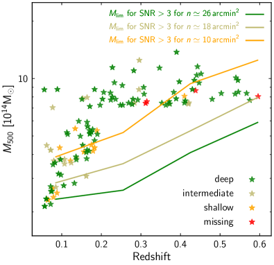
Figure 7: Lensing observational status. $M_{\rm 500}$–$z$ plane with symbol colours representing the depth of the archival or dedicated lensing data. Shallow surveys like CFIS (and more so, DES, KiDS) yielding a density of background sources $n\lesssim 10\,{\rm arcmin}^{-2}$ cannot probe the low mass end of Tier-1 clusters with ${\rm S/N}>3$. Stacking of the shear signal will be unavoidable for these. Deep Subaru data enable such measurements on individual clusters since most observations reach source densities $\gtrsim 20\,{\rm arcmin}^{-2}$. Euclid, which will reach $n\simeq 30\,{\rm arcmin}^{-2}$ will greatly simplify cluster mass calibrations with lensing.

4 Supporting data

4.1 Lensing

Accurate WL measurements of the matter distribution of the CHEX-MATE clusters are crucial to fulfilling the project goals. The homogeneous and complete WL coverage of the sample can be obtained by complementing high-quality optical archival data from ground based telescopes with dedicated proposals.

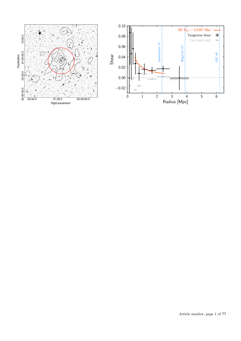
Figure 8: Left: MegaCam $r$-band optical image of the Tier-1 cluster PSZ2 G077.90-26.63 (A2409) of mass $M^{Y_{\rm SZ}}_{500}\simeq 5\times 10^{14}{\rm M_{\odot}}$ at redshift $z=0.148$, with convergence (i.e. surface mass density) contours overlaid. The red circle delimits $R_{500}$. Right: Radial shear profile obtained for PSZ2 G077.90-26.63, showing that, besides the ability to constrain the overall mass to within $30\%$ or so, only a modest handle on individual profile shapes is possible. The vertical lines show the outermost scale grasped by the main facilities we use for lensing, which nicely encompass the virial radius of most clusters, even at low redshift. In particular, the $0.5-2.5\,{\rm Mpc}$ range (radial span of the red curve) over which model fitting performs best, is well covered by our data. Grey points represent the curl component of the shear profile, which should be consistent with zero (error bars are not shown for clarity, but are the same as for the tangential component).

More than half of the sample, 62 clusters out of 118, have already been studied as part of various published WL analyses; these are detailed in the Literature Catalogs of weak Lensing Clusters of galaxies (LC²; Sereno 2015). Programmes including CLASH (Umetsu et al. 2014), WtG (Applegate et al. 2014), CCCP (Herbonnet et al. 2020), LoCuSS (Okabe & Smith 2016), or PSZ2LenS (Sereno et al. 2017) have shown that WL analyses can recover the mass up to a best accuracy of $\sim 20-25\%$ (including scatter due to triaxiality, substructures, intrinsic shape, and cosmic noise; e.g.Umetsu et al. 2016).

For lensing, the best possible multi-band optical wide field imaging is required. We thus consider observations with the 8.2-m Subaru telescope with the Hyper Suprime Cam (HSC) ($1.77\leavevmode\nobreak\ \deg^{2}$ FoV) and its SuprimeCam ($34\arcmin\times 27\arcmin$ FoV) precursor (Miyazaki et al. 2018; Komiyama et al. 2018; Furusawa et al. 2018; Kawanomoto et al. 2018; Miyazaki et al. 2002) along with MegaCam at the 3.6-m Canada-France-Hawaii Telescope (CFHT) ($1\deg^{2}$ FoV) , both located at the Mauna Kea summit (Hawaii). For the Southern hemisphere, the OmegaCam at the 2.5-m VLT Survey Telescope (VST) on Paranal (Chile) ($1\deg^{2}$ FoV) and the Wide Field Imager (WFI) at the 2.2-m MPG/ESO ($0.25\deg^{2}$ FoV) telescope at La Silla (Chile) are also considered. Good partial or complete data sets are already available from these archives for 83 clusters.

Additionally, two ongoing surveys are of particular interest for the CHEX-MATE program. The Hyper Suprime-Cam Subaru Strategic Program (HSC-SSP, Miyazaki et al. 2018; Aihara et al. 2018) has been carrying out a multi-band imaging survey in five optical bands ($grizy$) with a depth of $i\sim 26$ at the $5\sigma$ limit within a 2″ diameter aperture, aimed at observing $\sim 1400\deg^{2}$ on the sky in its Wide layer (Aihara et al. 2018). The survey is optimised for WL studies (Mandelbaum et al. 2018; Hikage et al. 2019; Miyatake et al. 2019; Hamana et al. 2020; Okabe et al. 2020) and should be completed in 2021. Five CHEX-MATE clusters fall in the HSC-SPP footprint. CFIS is an ongoing legacy programme at the CFHT (Ibata et al. 2017). It is part of a wider multi-band imaging effort named UNIONS, which is underway to map the Northern extragalactic sky, notably to support the Euclid space mission. To aid the follow-up of CHEX-MATE, 33 Tier-1 clusters have expressly been selected to lie in the CFIS footprint. About $\sim 4500\,\deg^{2}$ will be obtained in the r-band to a depth of 24.1 (point source, S/N=10, 2″ diameter aperture) with a median seeing of $0\aas@@fstack{\prime\prime}66$. As of now, $2500\,\deg^{2}$ are already available and full completion may require another two years of observations. CFIS observations in the u-band (mag${}_{\rm lim}\sim 23.6$, median seeing $0\aas@@fstack{\prime\prime}85$), are not deep enough to bring significant photometric information for the background sources but will aid our understanding of the star formation in cluster member galaxies. Likewise, complementary z band data coverage in the UNIONS collaboration is being obtained with good image quality from Subaru (WISHES program, PI M. Oguri), which has also started to observe the same footprint to a magnitude of 23.4 (same definition as above). This is comparable to the r-band depth, and can thus be helpful for the stellar mass content of cluster member galaxies as well as for the redshift estimation of the faint background sources. In total, 34 clusters (nine unique clusters covered neither by archival data nor dedicated proposals) fall in these two survey footprints.

The data set will be completed with targeted observations of 31 clusters from dedicated proposals (26 unique clusters not covered at all by archival data) or ongoing WL surveys for 34 clusters (nine unique clusters). The CHEX-MATE collaboration has already been awarded $\sim 32$ h at HSC@Subaru (proposals S19B-TE220-K, S20A-TE129-KQ, S20B-TE212-KQ, P.I. J. Sayers), $\sim 21$ h at Megacam@CFHT (P.I. R. Gavazzi/K. Umetsu), and $\sim 23$ h at OmegaCam@VST (proposals 0104.A-0255(A) and 105.2095.001, P.I. M. Sereno). A partial summary of already available observations is reported in Table C. Some redundancy in available data is present and this will be exploited to assert our control of systematics in shear measurements by requiring consistency between lensing data measured with HSC and Megacam for instance. A full assessment of the quality and internal consistency of the lensing measurement will be addressed in specific papers.

Arguably, the driving criterion for obtaining accurate lensing measurements is the surface number density of background, potentially lensed, sources, lying far behind the foreground massive cluster. With observations with integration time of $\sim$ 30 minutes at an 8-metre class telescope, source densities as high as $n_{\rm bg}\simeq 20\,{\rm arcmin}^{-2}$ (eg Medezinski et al. 2018) can be obtained. Hence, the lensing signal from regions up to $\sim 2-3\leavevmode\nobreak\ \text{Mpc}$ can be recovered with an S/N$\sim 5-10$ (Applegate et al. 2014; Okabe & Smith 2016; Umetsu et al. 2016). For comparison, Euclid space-borne imaging should routinely yield densities $n_{\rm bg}\simeq 30\,{\rm arcmin}^{-2}$. With CFHT and similar telescopes, reaching the same depth is more difficult and most often lensing data deliver $n_{\rm bg}\sim 9-15\,{\rm arcmin}^{-2}$, (with a 30-60 minute integration time). This is particularly true for CFIS. Shallower surveys like KiDS or DES do not exceed $n_{\rm bg}\sim 8\,{\rm arcmin}^{-2}$. The point spread function represents an additional problem for ground-based observations, as an increase in the number of blended sources reduces the number of galaxies that can be used for WL. As shown in Fig. 7, deep observations corresponding to the best images ($t>30$ min on Subaru) and observations of intermediate depth ($30>t>10$ min on Subaru-equivalent telescopes) should enable individual mass measurements of 33% accuracy or better for most Tier-1 and all Tier-2 clusters. The shallower data ($t<10$ min on Subaru-equivalent) will not permit such mass determinations on individual clusters, so one would have to resort to stacking techniques in order to put constraints on the lowest mass end ($M_{500}\lesssim 3\times 10^{14}\,{\rm M_{\odot}}$) of Tier-1 clusters.

Depth is not the only criterion, however. Some amount of colour information on background sources is required for efficient and clean separation of background galaxies from cluster members and foreground sources. A two-band colour selection is needed for clusters at $z\la 0.2$, whereas three bands are needed for more distant clusters. With this requirement, we are able to control contamination by cluster member galaxies at the percent level (Okabe & Smith 2016) and, whenever needed, our dedicated observations will obtain this minimal coverage. For many of the well-known Tier-2 clusters, several more bands are often available (uBV, Rc, I, z), and will be used.

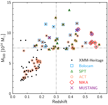
Figure 9: Current SZE coverage by various facilities of the CHEX-MATE sample in the $M_{500}-z$ plane. The details are given in Table 10 and are further discussed in Sect. 4.2.

In addition to an overall mass measurement, WL can also provide information on the mass density profile if the density of background sources is large enough ($n\gtrsim 20\,{\rm arcmin}^{-2}$). The right-hand panel of Fig. 8 shows the radial shear profile one can obtain under the typical observing conditions we expect. The example is PSZ2  G$077.90-26.63$ (A2409) at $z=0.148$, for which deep SuprimeCam data yields $n=22$ faint background galaxies per square arc minute out to about 2.5 Mpc from the centre. The accuracy on mass is 33% for a mass of order $M_{500}\simeq 5\times 10^{14}{\rm M_{\odot}}$. We typically expect the shear signal to deliver constraints on the concentration of individual halos to 30% accuracy for the most massive clusters, with a source density $n\gtrsim 20\,{\rm arcmin}^{-2}$. On the other hand, for low-mass, Tier-1 clusters, with the shallowest (CFIS or DES-like) observations, the same accuracy can only be achieved after the stacking of about 20 clusters or so. In this process, we intend to stack the likelihood in a hierarchical Bayesian manner (see eg Lieu et al. 2017) rather than use a crude shear stacking in concentric annuli.

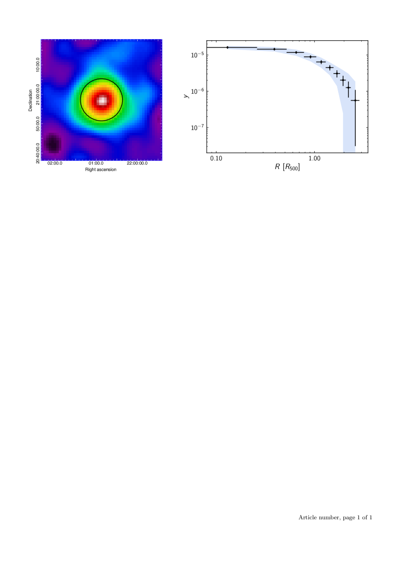
Figure 10: Left: Planck Comptonisation $y$ map of the Tier-1 cluster PSZ2 G077.90-26.63. The black circle represents $R_{500}$. Right: Radial SZE profile in Comptonisation parameter, $y$, and radial units of $R_{500}$. The profile is derived from the $y$-map following the method published in Planck Collaboration Int. V (2013). The individual points are correlated at about the 20% level and the error bars show the square root of the diagonal elements from the covariance matrix. The blue shaded envelope shows the dispersion in flux about the profile.

4.2 Sunyaev-Zeldovich effect

As stressed above, the SZE data are complementary to the X-ray data, providing an independent tracer of the hot intra-cluster gas. Our sample of 118 clusters was selected from the Planck all-sky survey (Planck Collaboration I 2016) with a S/N $>6.5$. We therefore have high-quality Planck SZE data for all of the targets. For example, from the public Planck all-sky Modified Internal Linear Combination Algorithm (MILCA) SZE map (Planck Collaboration XXII 2016), we can obtain the radial distribution of the SZE signal for each object in our sample. From further deprojection and deconvolution, we can also reconstruct the underlying 3D gas pressure profile following the methodology developed by Planck Collaboration V (2013). In conjunction with the XMM-Newton data, these Planck-derived constraints will provide further insights into the scaling and structural properties of the galaxy cluster population.

For the 61 Tier-1 clusters at $z<0.2$, the Planck data alone are likely to be sufficient for most desired analyses. For the higher-$z$ Tier-2 clusters, many potential analyses will benefit from the inclusion of higher angular resolution SZE data from wide-field ground-based facilities (see, e.g. Sayers et al. 2016; Ruppin et al. 2018). In particular, data are publicly available from Bolocam (Sayers et al. 2013), the SPT-SZ survey (Chown et al. 2018), and the ACT surveys (Aiola et al. 2020). In total, these data include 43 unique Tier-2 clusters (and 21 unique Tier-1 clusters), some with coverage from more than one data set. In the relatively near future, we also expect data releases from the SPT-ECS survey (Bleem et al. 2020) and the New Iram Kids Array (NIKA2) SZ Large Program (Mayet et al. 2020). In total, these data will include five additional unique Tier-2 clusters. A summary of the available SZE data is given in Figure 9 and Table 10.

Beyond these wide-field SZE data, which generally have an angular resolution of $\sim 1$ arcminute, ground-based SZE observations with spatial resolution comparable to the X-ray data could provide a transformational added value. Joint X-ray and SZE analyses would allow detailed reconstructions of the internal structure of the physical properties of the hot gas (e.g. Adam et al. 2017; Ruppin et al. 2018). In particular, NIKA2 (Perotto et al. 2020) and MUSTANG-2 (Dicker et al. 2014), currently operating on the Institut de Radioastronomie Millimétrique (IRAM) 30m and Green Bank Telescope (GBT) 100m telescopes, obtain 18 and 9 arcsec FWHM resolutions at 150 and 90 GHz, respectively.

Even higher resolution SZE observations are possible with current large interferometric observatories such as the Atacama Large Millimetre Array (ALMA) and the Northern Extended Millimeter Array) NOEMA (see, e.g. Kitayama et al. 2016). Accounting for the limited coverage provided by these facilities, such observations would target, within a reasonable exposure time, specific regions for either a single cluster or a sample of targets; for example, a follow-up of shocks or any other spatial feature of interest (Basu et al. 2016; Kitayama et al. 2020).

From the combination of the SZE data from Planck, along with publicly available data from Bolocam, SPT, ACT, and NIKA2, we will derive global SZE properties such as $Y_{SZ}=\int yd\Omega$, where the Compton $y$ parameter is integrated over the aperture $\Omega$ obtained from the X-ray XMM-Newton analysis (centroid, $R_{500}$, etc.) to construct scaling relations (e.g. $Y_{X}-Y_{SZ}$) for the entire sample. Revisiting previous works (e.g. Planck Collaboration X 2011; Planck Collaboration XI 2011), this will provide a solid local reference from an SZE selected sample covering the full mass range (Tier-1) and and from a mass-limited sample at low-to-intermediate redshift (Tier-2). In addition, joint X-ray and SZE analyses, building on what was performed for the X-COP and CLASH projects (Eckert et al. 2017; Siegel et al. 2018; Sereno et al. 2018), will provide a complementary view to standalone X-ray analyses of the structural thermodynamical properties beyond $R_{500}$ and into the clusters’ outskirts. High-resolution SZE images will be also instrumental in constraining the ICM power spectrum jointly with X-ray images (e.g. Khatri & Gaspari 2016). An example image and radial profile of PSZ2 G077.9-26.63, obtained from the Planck survey data, is shown in Fig. 10.

We would ideally like to obtain SZE data with an angular resolution comparable to the XMM-Newton X-ray images. The complementarity of these multi-probe data would allow for detailed studies of sub-structures within the ICM (see e.g. the recent combination of XMM-Newton and NIKA2 or MUSTANG data by Ruppin et al. 2018, Okabe et al. 2020, and Kéruzoré et al. 2020). As noted above, both NIKA2 and MUSTANG-2 can provide such data and are available for open-time observations. For both instruments the integration time goes from reasonable (a few hours) to relatively time consuming ($\sim$10-20h per targets) depending on the mass and redshift of the cluster. For example, NIKA2 could provide images extending to $R_{500}$ of clusters at $z=0.3$ in approximately three hours for $M_{500}=15\times 10^{14}$ M_⊙ and in approximately 18 hours for $M_{500}=7\times 10^{14}$ M_⊙. Based on realistic open-time requests, and actual allocations to other large cluster programs (e.g. Mayet et al. 2020; Dicker et al. 2020), obtaining coverage for sub-samples of $\lesssim 10$ clusters is possible. We will thus pursue MUSTANG-2 and NIKA2 imaging of well-defined sub-samples, or individual targets, where the high angular resolution SZE data will have the most impact. In addition, such followup will be pursued to cover the 13 remaining Tier-2 clusters that lack ground-based follow-up.

4.3 Chandra X-ray

Accompanying Chandra data for the CHEX-MATE clusters will be of importance in the completion of certain project goals. In particular, its high spatial resolution is preferred for studying the central regions of clusters (within  100 kpc of the centre). This will be crucial when it comes to detecting the presence of cavities and other key AGN feedback features, along with studying and mapping the thermodynamic properties of the core. Chandra observations will also be used to detect and characterise point sources that are unresolved in the XMM-Newton data (their expected variability in X-ray flux between observation epochs notwithstanding; Maughan & Reiprich 2019).

At the time of writing, 101/118 galaxy clusters in the sample have available Chandra data. Additionally, public data for PSZ2 G004.45-19.55 should be available soon, and PSZ2 G111.75+70.37 is within the field of view of a scheduled observation. However, the only available data for PSZ2 G067.52+34.75 (ObsID 14988) is unsuitable for galaxy cluster science, as not only is the observation limited to a single ACIS-S chip, but it also has a restrictive custom sub-array applied.

The Chandra coverage is representative of the full sample in mass and should be sufficient for the goals described above. In general, the data quality across the sample is good, with a minimum depth of ¿1600 counts (between 0.6 and 9.0 keV) within $R_{500}$. This is comparable to the data quality used for cavity searches in Hlavacek-Larrondo et al. (2015). In the central 100 kpc, this translates to a median data quality of $\sim$1700 counts in the 0.7-2.0 keV energy band.

4.4 Radio

Radio observations of galaxy clusters show several types of sources connected to the ICM (see van Weeren et al. 2019 for a recent review). Radio halos are Mpc-size sources located at the cluster centres and are possibly due to turbulent re-acceleration during major mergers. Radio relics are arc-like radio sources located at the cluster periphery and linked to shock (re)accelerations. Mini-halos are sources of a few hundred kpc in size found at the centre of cool-core clusters surrounding the bright radio-loud BCG (Gitti et al. 2018).

To understand the origin of radio halos and relics, it is important to quantify their occurrence as a function of cluster mass, redshift, and dynamical state. The CHEX-MATE samples represent good starting point for this analysis, which will complement the mass-complete samples already studied or planned (Cassano et al. 2013; Cuciti et al. 2015). Despite the number of archival observations in the radio band, the different sensitivity and observing bands of the clusters do not permit us to derive firm conclusions on the occurrence and evolution of radio halos and relics. The fraction of clusters known to host a radio halo, relic, or mini halo in Tiers-1 and 2 are listed in Table 3. In the coming years, radio surveys with new and up-coming facilities will provide data with homogeneous sensitivity to cluster diffuse emission, allowing one to perform unbiased statistical studies on the occurrence of radio halos, relics, and mini halos, and on their evolution with time.

Sample	Radio halos	Radio relics	Mini halos
Tier-1	7%	3%	10%
Tier-2	39 %	5%	5%

Table 3: Fraction of clusters with known diffuse radio sources for each Tier.

Specifically, the Low Frequency Array (LOFAR) Two-metre Sky Survey (LoTSS, Shimwell et al. 2019) will observe the Northern sky with unprecedented sensitivity ($\leq 100\leavevmode\nobreak\ \mu$Jy/beam) and resolution ($6"$) at low radio frequency 120-168 MHz, providing a complete view of non-thermal phenomena in galaxy clusters. All CHEX-MATE clusters at DEC$>0$; that is, 82 of 118 objects, would have a guaranteed LOFAR follow-up in the framework of LoTSS. Sixty clusters have already been observed by LoTSS at the time of writing. In the Southern sky, other surveys are providing a homogeneous coverage of clusters. These include the GaLactic and Extragalactic All-sky MWA survey (GLEAM, George et al. 2017), undertaken with the Murchison Widefield Array, and the Evolutionary Map of the Universe survey (EMU, Norris 2011), undertaken with the Australian Square Kilometre Array Pathfinder. These will complement LoTSS with a similar resolution and sensitivity to extended cluster radio emission. The GLEAM survey (and EMU in the coming years) covers the entire sky south of DEC$>+30$ and is thus expected to provide a radio coverage of about 86 clusters.

4.5 Hydrodynamical cluster simulations

In addition to the multi-wavelength observational data, theoretical input to CHEX-MATE will also be furnished with a large suite of hydrodynamical simulations of galaxy clusters, providing unprecedented statistics of these massive objects. The simulations are crucial for two main reasons. Firstly, they can be used for interpreting the observational data to further our understanding of cluster physics; for example, models of chemical enrichment, stellar and black hole feedback, magnetic fields, and hydrodynamical processes such as viscosity, turbulence and conduction. This will be achieved through comparison of observed and simulated cluster properties such as radial profiles (e.g. entropy, temperature, pressure and metallicity) and global scaling relations between observables (e.g. X-ray luminosity, temperature, SZE flux) and cluster mass within different apertures. For the latter, this will include mass estimates from simulated X-ray, SZE and lensing profiles, as well as their true values. Secondly, they are being used to study the effects of cluster selection; for example, comparing clusters selected with SZE versus X-ray flux and assessing the impact of large-scale structure along the line-of-sight, as well as allowing simulated cluster samples with similar characteristics to the observed sample (e.g. in mass, redshift and morphology) to be identified. We are also looking at related issues, such as cluster centring, classifying clusters using various dynamical and structural estimators, and investigating the level of hydrostatic mass bias (including how it is estimated, and how it depends on mass, redshift and dynamical state).

Simulation data are initially being provided using a number of existing data sets. In particular, we are using The Three Hundred (Cui et al. 2018), BAHAMAS+MACSIS (McCarthy et al. 2017; Barnes et al. 2017b) and Magneticum (Dolag et al. 2016) simulations as these contain significant numbers of clusters that occupy the relevant regions of mass-redshift space for both Tier-1 and Tier-2 samples (e.g. the largest Magneticum box contains over 200 thousand clusters in the Tier-1 mass range at redshift, $z=0$, and over 300 in the Tier-2 mass range at $z\simeq 0.5$). These simulations are supplemented with a wide range of other runs available within the collaboration, which are also very useful for addressing specific science projects using the CHEX-MATE data (e.g. Barnes et al. 2017a, 2018; Gaspari et al. 2018; Le Brun et al. 2018; Rasia et al. 2015; Ruppin et al. 2019; Vazza et al. 2017). Beyond this, we will investigate the creation of bespoke simulated cluster samples for CHEX-MATE, taking into account both the latest cluster physics models and simulation codes available to the collaboration. High-resolution simulations will be also useful to generate detailed synthetic maps with different systematic and statistical errors and instrument responses.

5 Summary and conclusions

The CHEX-MATE sample of 118 systems has been built as a future reference for clusters in the local volume and in the high mass regime. Its unique construction ensures that it contains not only the objects that make up the bulk of the population, but also the most massive systems, which are the most interesting targets for detailed multi-wavelength follow-up. The project is intended to yield fundamental insights into the cluster mass scale and its relationship to the baryonic observables. It is conceived to be the key reference for numerical simulations, providing an observational calibration of the scaling laws between baryonic quantities and the underlying mass; it will provide the ultimate overview of the structural properties; and it will uncover the links between global and structural properties and the dynamical state and the presence of central cooling gas.

A high-quality, homogeneous data set is critical in order to fulfil these objectives. We have detailed the X-ray observation preparation, exposure time calculation, and data analysis procedures needed to obtain the desired result, and we have shown that the new observations obtained for the project are in line with expectations. Although the X-ray observations are the backbone of the project, it is intrinsically multi-wavelength in nature. The majority of the sample is already covered by an extremely rich data set comprising multi-band optical, SZE, and radio observations. Through its various working groups, the CHEX-MATE collaboration has embarked upon a considerable effort to completing this multi-wavelength follow-up. A parallel numerical simulation effort is also being undertaken.

The project legacy will be considerable. The sample corresponds to the descendants of the high–$z$ clusters that will be detected by upcoming SZE surveys such as SPT-3G, and the project will also provide key input for the interpretation of eROSITA survey data. Ultimately, we would like a method to detect clusters based on their most fundamental property: the total mass. This is becoming possible through WL analysis of the increasingly available high-quality, large-area, multi-band optical imaging data sets. Our project has particular synergy with Euclid, the sensitivity of which should allow blind detection of objects uniquely through their WL signal in the redshift and mass range covered by our sample. In the longer term, our sample will provide the targets of reference for dedicated Athena pointings for the deep exploration of ICM physics.

CHEX-MATE represents a very large investment of XMM-Newton exposure time. The data are intended to be a community resource, and as such the X-ray observations do not have a proprietary period. They may be downloaded from the XMM-Newton archive immediately after they have been obtained and processed by the XMM-Newton SOC. This paper includes the first public release of the CHEX-MATE source list and X-ray observation details. Our hope is that the sample will be the foundation for cluster science with next-generation instruments for many years to come, fully justifying the investment in XMM-Newton observing time and providing a unique heritage for ESA’s most successful astronomy mission.

Appendix A Sample selection strategy

A.1 Detailed selection strategy

Figure 11 illustrates the sample selection strategy. Starting from the PSZ2 catalogue, clusters that were successively removed owing to various criteria are marked in the $z$–$M_{500}$ plane, where $M_{500}$ is the PSZ2 mass.

The first selection step is based on criteria that depend on source position on the sky, and is illustrated in the top panels. Sources outside the Planck cosmological mask, or with XMM-Newton visibility less than 55 ksec were first excluded. Those with known redshift are marked by red crosses and orange points, respectively, in the top-left panel. The clusters remaining after this selection are shown with black points in the right panel; excluded clusters are shown in grey. We note that the XMM-Newton visibility criterion depends only on the object position in the sky. The region excluded by the visibility criterion is shown as a pink shaded area in Fig. 2.

The second selection step is based on a criterion that depends on the S/N of the Planck SZE detection by the MMF3 algorithm. In the left-middle panel, sources that met the previous criteria but that are at ${\rm S/N_{MMF3}}<6.5$ are marked with magenta crosses. Objects excluded in this and the first step are shown in grey in the middle-right panel. The remaining clusters are marked with black points; these, plus two not yet validated cluster candidates, comprise the parent cluster sample used for the definition of Tier-1 and Tier-2.

The bottom-left panel identifies the Tier-1 clusters with blue crosses. These are the clusters of the parent sample (black points) that are in the redshift range $0.05<z<0.2$, delimited by the blue shaded region, and in the northern sky (${\rm Dec}>0$). Objects in the blue region but not marked in blue correspond to clusters in the southern sky.

The bottom-right panel identifies the Tier-2 clusters with red plusses. These are the clusters of the parent sample (black points) that are in the redshift range $z<0.6$ and with mass $M_{\rm 500,MMF3}$, derived from the MMF3 detection, greater than $7.25\times 10^{14}{\rm M_{\odot}}$. The red shaded area delimits the corresponding region in the $z$–$M_{500}$ plane. The PSZ2 catalogue mass, $M_{500}$, was derived from the detection method that yielded the highest S/N. The nine clusters not marked by red plusses in the orange area have been detected at higher S/N by methods other than MMF3, but have $M_{\rm 500,MMF3}<7.25\times 10^{14}{\rm M_{\odot}}$.

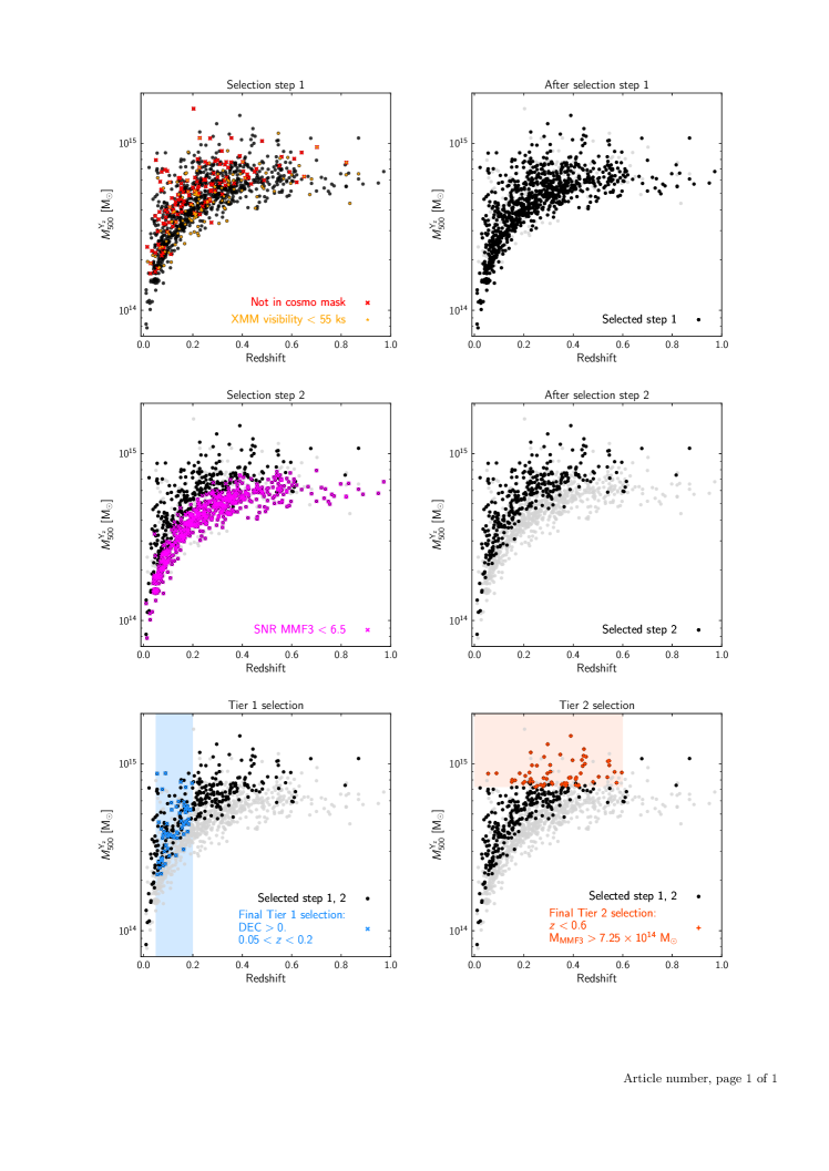
Figure 11: Sample selection strategy. See Appendix A for a detailed explanation.

A.2 Original selection

The total exposure time available in the original call for XMM-Newton Multi-Year Heritage programmes was 6 Msec. Our proposal was one of two programmes selected, and the total time was divided equally between them. Originally, we applied for 6 Msec to observe 169 (instead of 118) clusters. These objects were selected from the PSZ2 catalogue at S/N$>$6, and divided into two Tiers. Tier-1 consisted of 85 objects at $z<0.2$ with median $M_{500}$ of $3.7\times 10^{14}{\rm M_{\odot}}$. Tier-2 contained 84 systems at $z<0.6$ with $M_{500}>7\times 10^{14}{\rm M_{\odot}}$. There were seven objects in common between the two Tiers. To accommodate the reduction in allocated exposure time, and maintain our ability to work with our original goal of a ‘large, unbiased, signal-to-noise-limited sample’ we made several changes to the original object selection strategy. We raised the S/N cut to 6.5; we imposed a lower redshift cut of $z>0.05$ on the Tier-1 systems, which would have required deep off-axis observations to cover their emission up to $R_{500}$); we imposed a higher mass cut of $M_{500}>7.25\times 10^{14}{\rm M_{\odot}}$ on the Tier-2 sample.

After making these changes, the net reduction of 50% in exposure time corresponded to a reduction of about 30% in the number of objects.

Appendix B List of targets

Tables 3.2.1, 3.2.1, and 3.2.1 list the CHEX-MATE observations. They detail the following: the PSZ2 name; the coordinates of the X-ray peak in RA and Dec; the redshift; the nominal $M_{500}$ from the PSZ2 catalogue in units of $10^{14}\,{\rm M_{\odot}}$; the signal-to-noise ratio (S/N); the Tier to which the object belongs (either 1 or 2, or ‘12’ when the object belongs to both Tiers); the nominal Galactic absorption in units of $10^{20}\,{\rm cm}^{-2}$; the archived XMM-Newton exposure time in kiloseconds; the archived Chandra exposure time in kiloseconds; the requested new XMM-Newton exposure time in kiloseconds; the OBSid that identifies the observations used for the analysis (new exposures highlighted in bold font).

Table 4: List of CHEX-MATE XMM-Newton observations. We quote: the PSZ2 name; the coordinates of the X-ray peak; the redshift; the nominal $M_{500}$ from the PSZ2 catalogue; the Signal-to-Noise ratio; the Tier to which the object belongs (either 1 or 2; ”12” when the object is part of both Tiers); the nominal Galactic absorption; the archived XMM-Newton exposure time; the archived Chandra exposure time; the requested new XMM-Newton exposure time; the OBSid that identifies the observations used for the analysis (in bold font, the new exposures available on September 9 2020; the symbol ^⋆ identifies the targets that will be re-observed in the final year).

Name	RA	Dec	$z$	$M_{500}$	SNR	Tier	$n_{H}$	$t_{\rm XMM}$	$t_{\rm CXO}$	$t_{\rm XMM,new}$	OBSid
	h:m:s	d:m:s		$10^{14}M_{\odot}$			$10^{20}$ cm-2	ksec	ksec	ksec
PSZ2 G071.63+29.78	17:47:14.0	+45:11:45	0.1565	4.1	8.7	1	2.7	19.0	22.6	22.0	0692932201 0827050501
PSZ2 G072.62+41.46	16:40:19.9	+46:42:39	0.2280	11.4	27.4	2	1.8	40.1	497.4	0.0	0112231801 0112231901 0605000501
PSZ2 G073.97-27.82	21:53:36.8	+17:41:41	0.2329	9.5	19.1	2	6.2	20.0	115.4	21.0	0111270101
PSZ2 G075.71+13.51	19:21:12.0	+43:56:49	0.0557	8.7	49.0	12	8.1	81.9	90.8	0.0	030215(01-02)01 0600040101 0743840201 074441(01-03)01 0763490301
PSZ2 G077.90-26.63	22:00:52.5	+20:58:04	0.1470	5.0	11.1	1	6.6	0.0	10.4	23.0	0827020101
PSZ2 G080.16+57.65	15:01:07.9	+47:16:35	0.0878	2.5	7.8	1	2.5	0.0	0.0	29.0	0821040401⋆
PSZ2 G080.37+14.64	19:26:10.0	+48:33:10	0.0980	3.1	8.1	1	6.9	0.0	0.0	29.0	0827031501⋆
PSZ2 G080.41-33.24	22:26:06.1	+17:21:45	0.1072	3.8	8.7	1	5.1	108.8	124.8	0.0	0762470101
PSZ2 G083.29-31.03	22:28:33.7	+20:37:16	0.4120	7.6	9.5	2	4.3	22.3	20.1	30.0	0147890101 0827360901
PSZ2 G083.86+85.09	13:05:51.2	+30:53:42	0.1832	4.7	8.0	1	1.0	0.0	0.0	31.0	0827030701
PSZ2 G085.98+26.69	18:19:54.2	+57:09:22	0.1790	4.2	9.3	1	3.9	35.0	34.8	42.0	0692932701 0827041601
PSZ2 G087.03-57.37	23:37:37.5	+00:16:07	0.2779	7.3	11.2	2	3.5	9.0	26.4	22.0	0042341301
PSZ2 G092.71+73.46	13:35:18.2	+41:00:06	0.2279	8.0	17.6	2	0.8	23.1	95.9	21.0	0084230901
PSZ2 G094.69+26.36	18:32:30.9	+64:49:53	0.1623	3.1	7.7	1	4.4	19.7	0.0	53.0	0762801101
PSZ2 G098.44+56.59	14:27:25.4	+55:44:27	0.1318	2.8	6.6	1	1.3	0.0	0.0	48.0
PSZ2 G099.48+55.60	14:28:38.0	+56:51:35	0.1051	2.7	8.1	1	1.3	0.0	15.0	30.0	0821810901
PSZ2 G105.55+77.21	13:11:08.7	+39:13:37	0.0720	2.2	6.9	1	1.2	0.0	26.8	24.0	0827031301
PSZ2 G106.87-83.23	00:43:24.6	-20:37:16	0.2924	7.7	12.7	2	1.8	10.0	405.6	21.0	0042340201 0827041501
PSZ2 G107.10+65.32	13:32:45.4	+50:32:05	0.2799	7.8	16.5	2	1.0	55.3	235.6	0.0	0142860201
PSZ2 G111.61-45.71	00:18:33.2	+16:26:10	0.5456	8.5	9.7	2	4.0	32.3	68.3	26.0	0111000101 0111000201 0827061301
PSZ2 G111.75+70.37	13:13:06.4	+46:16:51	0.1830	4.3	8.3	1	1.1	0.0	0.0	36.0	0827020801
PSZ2 G113.29-29.69	00:11:45.9	+32:24:51	0.1073	3.6	8.1	1	4.7	0.0	8.1	21.0	0827021201
PSZ2 G113.91-37.01	00:19:41.7	+25:18:05	0.3712	7.6	8.2	2	2.9	0.0	0.0	49.0	0827021001
PSZ2 G114.79-33.71	00:20:37.5	+28:39:32	0.0940	3.8	9.4	1	3.9	0.0	14.1	21.0	0827320401
PSZ2 G124.20-36.48	00:55:50.6	+26:24:36	0.1971	7.3	12.8	12	5.4	40.7	366.3	0.0	0203220101
PSZ2 G143.26+65.24	11:59:14.8	+49:47:33	0.3634	7.3	10.2	2	2.2	0.0	22.1	45.0	0827020201 0827320201
PSZ2 G149.39-36.84	02:21:33.6	+21:21:42	0.1700	5.3	7.3	1	7.5	0.0	0.0	28.0	0827030601
PSZ2 G155.27-68.42	01:37:24.8	-08:27:20	0.5670	8.4	8.0	2	3.5	24.9	0.0	51.0	06936628(01-02) 0700180201 0827060801
PSZ2 G159.91-73.50	01:31:52.6	-13:36:43	0.2060	8.5	17.1	2	1.4	63.7	20.2	0.0	0084230301 0550960101
PSZ2 G172.74+65.30	11:11:40.4	+40:50:14	0.0794	2.4	7.5	1	1.3	0.0	11.7	23.0	0827031101
PSZ2 G172.98-53.55	02:39:53.3	-01:34:44	0.3730	7.4	7.6	2	3.0	130.0	96.3	0.0	0782150101
PSZ2 G179.09+60.12	10:40:44.5	+39:57:11	0.1372	3.8	7.5	1	1.7	36.6	58.1	27.0	0147630101 0827330401
PSZ2 G186.37+37.26	08:42:57.2	+36:22:03	0.2820	11.0	18.9	2	2.9	22.4	27.9	21.0	0605000701 0827041001
PSZ2 G187.53+21.92	07:32:20.4	+31:37:59	0.1710	5.2	8.1	1	4.9	18.6	217.6	21.0	0673850201
PSZ2 G192.18+56.12	10:16:21.9	+33:38:26	0.1240	3.6	7.8	1	1.5	0.0	5.1	25.0	0821810701
PSZ2 G195.75-24.32	04:54:06.5	+02:54:25	0.2030	7.8	11.8	2	5.7	42.4	535.2	0.0	0201510101
PSZ2 G201.50-27.31	04:54:11.1	-03:00:58	0.5377	8.3	7.1	2	3.9	42.6	58.8	56.0	0205670101 0827061001
PSZ2 G204.10+16.51	07:35:47.5	+15:06:48	0.1220	3.7	6.7	1	5.0	0.0	0.0	28.0	0827040401
PSZ2 G205.93-39.46	04:17:34.1	-11:54:18	0.4430	11.5	13.8	2	3.3	0.0	90.3	26.0	0827010101 0827011501 0827310101
PSZ2 G206.45+13.89	07:29:50.7	+11:56:28	0.4100	7.5	7.3	2	5.8	25.0	0.0	51.0	0762440301

Table 5: List of XMM-Newton observations.

Name	RA	Dec	$z$	$M_{500}$	SNR	Tier	$n_{H}$	$t_{\rm XMM}$	$t_{\rm CXO}$	$t_{\rm XMM,new}$	OBSid
	h:m:s	d:m:s		$10^{14}M_{\odot}$			$10^{20}$ cm-2	ksec	ksec	ksec
PSZ2 G207.88+81.31	12:12:18.2	+27:33:05	0.3530	7.4	10.1	2	1.7	0.0	14.8	43.0	0827020301
PSZ2 G208.80-30.67	04:54:06.7	-10:13:08	0.2475	7.3	9.5	2	4.8	85.5	168.6	0.0	0603890101
PSZ2 G210.64+17.09	07:48:46.6	+09:40:00	0.4800	7.8	7.6	2	2.7	11.7	0.0	60.0	0658200501
PSZ2 G216.62+47.00	09:49:51.5	+17:07:09	0.3826	8.5	9.8	2	3.1	12.7	35.6	43.0	0723160201
PSZ2 G217.09+40.15	09:24:05.9	+14:10:26	0.1357	3.9	7.0	1	3.3	0.0	30.1	28.0	0827031001
PSZ2 G217.40+10.88	07:38:18.4	+01:02:15	0.1890	5.3	7.8	1	8.5	0.0	0.0	37.0	0827330201⋆
PSZ2 G218.59+71.31	11:29:54.5	+23:48:14	0.1371	3.8	7.2	1	1.2	0.0	0.0	30.0
PSZ2 G218.81+35.51	09:09:12.6	+10:58:32	0.1751	5.2	8.4	1	3.2	27.4	34.9	21.0	0605000901 0673850901
PSZ2 G224.00+69.33	11:23:57.6	+21:28:56	0.1904	5.1	8.8	1	1.6	0.0	20.1	27.0	0827020901
PSZ2 G225.93-19.99	06:00:08.1	-20:08:07	0.4350	9.8	12.4	2	4.9	9.0	0.0	26.0	0650381401 0827050601
PSZ2 G226.18+76.79	11:55:17.9	+23:24:18	0.1427	6.0	14.6	1	1.8	279.8	157.9	0.0	050269(01-02)01 055128(01-02)01
PSZ2 G228.16+75.20	11:49:35.1	+22:24:08	0.5450	9.8	11.4	2	1.9	24.7	370.2	42.0	0693661701 0827341301
PSZ2 G229.74+77.96	12:01:13.2	+23:06:21	0.2690	7.4	12.0	2	2.2	0.0	26.1	27.0	0821810501⋆
PSZ2 G238.69+63.26	11:12:54.3	+13:26:05	0.1690	4.2	7.3	1	1.6	50.0	93.2	0.0	0500760101
PSZ2 G239.27-26.01	05:53:28.4	-33:42:33	0.4300	8.8	12.2	2	3.3	0.0	85.1	49.0	0827010401⋆
PSZ2 G241.11-28.68	05:42:57.1	-35:59:49	0.4200	7.4	9.0	2	3.0	10.0	0.0	55.0	0656202001 0827050801
PSZ2 G243.15-73.84	01:59:02.7	-34:12:57	0.4100	8.1	10.3	2	1.5	0.0	19.5	48.0	0827011301
PSZ2 G243.64+67.74	11:32:51.9	+14:27:11	0.0834	3.6	12.0	1	2.9	0.0	9.1	21.0	0827010801
PSZ2 G259.98-63.43	02:32:18.7	-44:20:46	0.2836	7.5	13.0	2	1.7	10.0	23.7	21.0	0042340301
PSZ2 G262.27-35.38	05:16:37.4	-54:30:10	0.2952	8.8	22.9	2	2.1	58.1	31.4	0.0	0042340701 0205330301 0692934301
PSZ2 G262.73-40.92	04:38:17.4	-54:19:23	0.4210	7.5	12.7	2	1.0	14.7	20.0	42.0	0656201601
PSZ2 G263.68-22.55	06:45:28.8	-54:13:37	0.1644	8.0	21.7	2	5.6	47.4	10.1	0.0	0201901201 0201903401 0404910401
PSZ2 G266.04-21.25	06:58:30.0	-55:56:23	0.2965	12.5	28.4	2	4.9	38.7	584.2	0.0	0112980201
PSZ2 G266.83+25.08	10:23:50.2	-27:15:21	0.2542	7.3	11.7	2	5.6	0.0	37.2	29.0	0827011001
PSZ2 G271.18-30.95	05:49:19.6	-62:05:13	0.3700	7.4	14.1	2	4.5	10.0	0.0	46.0	0656201301 0827050701
PSZ2 G273.59+63.27	12:00:25.4	+03:20:49	0.1339	5.5	12.6	1	2.1	14.7	19.6	21.0	0827010301
PSZ2 G277.76-51.74	02:54:16.1	-58:56:52	0.4380	8.7	15.1	2	1.9	68.6	0.0	0.0	0656200301 0674380301
PSZ2 G278.58+39.16	11:31:54.2	-19:55:40	0.3075	8.3	12.2	2	4.0	10.0	99.2	21.0	0042341001
PSZ2 G283.91+73.87	10:16:21.9	+33:38:26	0.0852	2.7	8.4	1	2.1	0.0	42.0	21.0	0827330501
PSZ2 G284.41+52.45	12:06:12.0	-08:48:03	0.4414	10.4	13.6	2	4.3	178.9	203.8	0.0	0502430401 0762070101
PSZ2 G285.63+72.75	12:30:47.6	+10:33:11	0.1650	5.6	10.9	1	2.1	0.0	19.2	21.0	0827011101
PSZ2 G286.98+32.90	11:50:49.0	-28:04:28	0.3900	13.7	22.7	2	7.3	10.0	199.0	21.0	0656201201 0827341401
PSZ2 G287.46+81.12	12:41:17.6	+18:34:28	0.0730	2.6	7.4	1	1.5	15.5	0.0	0.0	0149900301
PSZ2 G313.33+61.13	13:11:29.3	-01:20:27	0.1832	8.8	16.7	2	1.8	84.8	199.8	0.0	0093030101 069382(01-02)01
PSZ2 G313.88-17.11	16:01:49.2	-75:45:14	0.1530	7.9	16.6	2	5.9	31.5	9.1	0.0	0692932001
PSZ2 G324.04+48.79	13:47:30.5	-11:45:07	0.4516	10.6	11.5	2	4.6	36.5	335.5	0.0	0112960101
PSZ2 G325.70+17.34	14:47:33.9	-40:20:38	0.3155	7.6	8.7	2	6.8	0.0	30.1	45.0	0827020701
PSZ2 G339.63-69.34	23:44:43.9	-42:43:11	0.5960	8.1	9.2	2	1.5	237.2	558.7	0.0	0693661801 072270(01-02)01
PSZ2 G340.36+60.58	14:01:02.2	+02:52:43	0.2528	9.2	15.6	2	2.0	368.4	363.7	0.0	0098010101 0147330201 055183(01-02)01
PSZ2 G340.94+35.07	14:59:29.0	-18:10:44	0.2357	7.8	10.5	2	7.4	0.0	40.2	24.0	0827311201
PSZ2 G346.61+35.06	15:15:03.1	-15:22:46	0.2226	8.4	12.9	2	8.3	0.0	60.0	21.0	0827010201⋆
PSZ2 G349.46-59.95	22:48:44.4	-44:31:58	0.3475	11.4	20.7	2	1.2	39.8	125.2	0.0	0504630101

Table 6: List of XMM-Newton observations.

Appendix C Weak lensing archive data

Tables C and C contain a summary of the archival optical data available for weak lensing (WL) observations as of winter 2019. We only considered observations with an exposure time rescaled to an equivalent Subaru dish area longer than three minutes. We also list which clusters form part of WL samples in the literature: CLASH-WL are the CLASH clusters with measured WL mass from Umetsu et al. (2016) or Merten et al. (2015); WtG from Applegate et al. (2014); CCCP100 is the combined CCCP plus MENeaCS sample from Herbonnet et al. (2020); LoCuSS from Okabe & Smith (2016); PSZ2LenS from Sereno et al. (2017); LC2 from $LC^{2}$ (Sereno 2015). The Table also contains information on WL surveys to be completed by 2022: the Hyper Suprime-Cam Subaru Strategic Program (Aihara et al. 2018, HSC-SSP); the CFHTLenS (Canada France Hawaii Telescope Lensing Survey, Heymans et al. 2012); RCSLenS (Red Cluster Sequence Lensing Survey, Hildebrandt et al. 2016); KiDS (Kilo-Degree Survey , de Jong et al. 2013); DES ( Dark Energy Survey , Dark Energy Survey Collaboration et al. 2016). For ongoing surveys, we considered the final planned footprint. The description of the relative broad band filters is presented in Table 9.

Table 7: Summary of archival data for weak lensing as of winter 2019. Columns 2-5: Available observations in multi-band filters at worldwide facilities, see Table 9. We only considered observations with an exposure time rescaled to an equivalent Subaru dish area longer than 3 minutes. Column 6: WL samples from literature; CLASH-WL are the CLASH clusters with measured WL mass from Umetsu et al. (2016) or Merten et al. (2015); WtG from Applegate et al. (2014); CCCP100 is the combined CCCP plus MENeaCS sample from Herbonnet et al. (2020); LoCuSS from Okabe & Smith (2016); PSZ2LenS from Sereno et al. (2017); LC2 from $LC^{2}$ (Sereno 2015). Column 7: WL surveys to be completed by 2022: the Hyper Suprime-Cam Subaru Strategic Program (Aihara et al. 2018, HSC-SSP); the CFHTLenS (Canada France Hawaii Telescope Lensing Survey, Heymans et al. 2012); RCSLenS (Red Cluster Sequence Lensing Survey, Hildebrandt et al. 2016); KiDS (Kilo-Degree Survey, de Jong et al. 2013); DES ( Dark Energy Survey, Dark Energy Survey Collaboration et al. 2016). For ongoing surveys, we considered the final planned footprint.

Name	SuP@Subaru	HSC@Subaru	Megacam@CFHT	OC@VST	HAWKI	WFI@MPG/ESO	WL samples	WL surveys
PSZ2 G000.13+78.04	–	–	–	–	–	–	–	–
PSZ2 G004.45-19.55	–	–	–	$i^{+}$	–	–	–	–
PSZ2 G006.49+50.56	–	–	$gri$	–	–	–	LC2,PSZ2LS,CCCP100	RCSLS
PSZ2 G008.31-64.74	–	–	–	$r^{+}i^{+}$	$J$	–	–	KiDS
PSZ2 G008.94-81.22	$B_{J}R_{C}i^{+}z^{+}$	–	$i$	$r^{+}i^{+}$	$K_{S}$	$B_{99}B_{J,842}V_{843}V_{89}R_{C,844}R_{C,162}I_{C,879}z^{+,846}$	LC2	KiDS,DES
PSZ2 G021.10+33.24	$V_{J}i^{+}$	–	$gr$	–	–	$B_{J,842}R_{C,844}I_{C,879}$	LC2,LoCuSS,WtG,CCCP100	–
PSZ2 G028.63+50.15	–	–	$r$	–	–	–	–	–
PSZ2 G028.89+60.13	$V_{J}R_{C}i^{+}$	–	–	–	–	–	LC2,LoCuSS	–
PSZ2 G031.93+78.71	–	–	$r$	–	–	–	–	–
PSZ2 G033.81+77.18	–	–	$gr$	–	–	–	LC2,CCCP100	–
PSZ2 G040.03+74.95	–	–	$r$	–	–	–	–	–
PSZ2 G040.58+77.12	–	–	$r$	–	–	–	–	–
PSZ2 G041.45+29.10	$V_{J}i^{+}$	–	–	–	–	–	–	–
PSZ2 G042.81+56.61	–	$i^{+}$	$gr$	–	–	–	LC2,CCCP100	–
PSZ2 G044.20+48.66	$g^{+}R_{C}$	–	$gr$	–	–	–	LC2,CCCP100	–
PSZ2 G044.77-51.30	$B_{J}V_{J}R_{C}I_{C}z^{+}$	–	$ur$	$r^{+}$	$JH$	–	LC2,WtG	–
PSZ2 G046.10+27.18	$B_{J}V_{J}R_{C}I_{C}z^{+}$	–	$ur$	–	–	–	LC2,WtG	–
PSZ2 G046.88+56.48	$V_{J}R_{C}i^{+}$	–	$gr$	–	–	–	LC2,CCCP100	–
PSZ2 G048.10+57.16	$g^{+}r^{+}i^{+}$	–	$ugr$	–	–	–	–	CFIS
PSZ2 G049.22+30.87	$V_{J}R_{C}$	–	–	–	–	–	LC2,LoCuSS,WtG	–
PSZ2 G049.32+44.37	–	–	$gr$	–	–	–	–	–
PSZ2 G050.40+31.17	$V_{J}i^{+}$	–	$gr$	–	–	–	LC2,CCCP100	–
PSZ2 G053.53+59.52	$B_{J}g^{+}R_{C}z^{+}$	–	–	–	–	–	LC2	CFIS
PSZ2 G055.59+31.85	$V_{J}R_{C}i^{+}$	–	$ugr$	–	–	–	LC2,CLASH-WL,LoCuSS,WtG,CCCP100	CFIS
PSZ2 G056.77+36.32	–	–	–	–	–	–	LC2	CFIS
PSZ2 G056.93-55.08	$B_{J}V_{J}R_{C}I_{C}z^{+}$	–	$ugri$	$r^{+}i^{+}$	–	–	LC2,WtG	–
PSZ2 G057.25-45.34	$B_{J}V_{J}R_{C}i^{+}I_{C}z^{+}$	–	$ur$	$r^{+}$	–	–	LC2,WtG	–
PSZ2 G057.61+34.93	–	–	$ugr$	–	–	–	–	CFIS
PSZ2 G057.78+52.32	–	–	–	–	–	–	–	CFIS
PSZ2 G057.92+27.64	–	–	–	–	–	–	–	CFIS
PSZ2 G062.46-21.35	–	–	$r$	–	–	–	–	–
PSZ2 G066.41+27.03	$i^{+}$	–	–	–	–	–	–	CFIS
PSZ2 G066.68+68.44	$V_{J}i^{+}$	–	$i$	–	–	–	–	CFIS
PSZ2 G067.17+67.46	$g^{+}V_{J}R_{C}i^{+}$	–	$gr$	–	–	–	LC2,LoCuSS,CCCP100	CFIS
PSZ2 G067.52+34.75	–	–	–	–	–	–	–	CFIS
PSZ2 G068.22+15.18	–	–	$r$	–	–	–	–	–
PSZ2 G071.63+29.78	–	–	–	–	–	–	–	CFIS
PSZ2 G072.62+41.46	$B_{J}V_{J}R_{C}i^{+}$	–	–	–	–	–	LC2,LoCuSS,WtG,CCCP100	CFIS
PSZ2 G073.97-27.82	$B_{J}V_{J}R_{C}i^{+}I_{C}z^{+}$	–	$u$	–	–	–	LC2,LoCuSS,WtG,CCCP100	–
PSZ2 G075.71+13.51	$B_{J}V_{J}R_{C}i^{+}$	$i^{+}$	$gr$	–	–	–	–	–
PSZ2 G077.90-26.63	$V_{J}i^{+}$	–	$gr$	–	–	–	–	–
PSZ2 G080.16+57.65	–	–	–	–	–	–	–	CFIS
PSZ2 G080.37+14.64	–	–	$r$	–	–	–	–	–
PSZ2 G080.41-33.24	–	–	$gr$	–	–	–	LC2,CCCP100	–
PSZ2 G083.29-31.03	$B_{J}R_{C}I_{C}z^{+}$	–	$ugri$	–	–	–	LC2,WtG	–
PSZ2 G083.86+85.09	$V_{J}$	–	–	–	–	–	–	CFIS
PSZ2 G085.98+26.69	–	–	$r$	–	–	–	–	CFIS
PSZ2 G087.03-57.37	$B_{J}V_{J}R_{C}i^{+}$	–	$ri$	–	–	$B_{J,842}V_{843}R_{C,844}$	LC2,PSZ2LS,LoCuSS,WtG	HSC-SSP,RCSLS,DES
PSZ2 G092.71+73.46	$V_{J}i^{+}$	–	–	–	–	–	LC2,LoCuSS,CCCP100	CFIS
PSZ2 G094.69+26.36	–	–	–	–	–	–	–	CFIS
PSZ2 G098.44+56.59	–	–	$ugri$	–	–	–	LC2,PSZ2LS	CFIS
PSZ2 G099.48+55.60	–	–	$ugri$	–	–	–	LC2,PSZ2LS	CFIS,CFHTLS
PSZ2 G105.55+77.21	–	$i^{+}$	$ugi$	–	–	–	–	CFIS
PSZ2 G106.87-83.23	$V_{J}i^{+}$	–	–	–	–	$B_{J,842}B_{J,878}V_{843}R_{C,844}$	LC2,LoCuSS	DES
PSZ2 G107.10+65.32	$B_{J}g^{+}V_{J}R_{C}i^{+}z^{+}$	–	$gr$	–	–	–	LC2,LoCuSS,WtG,CCCP100	CFIS
PSZ2 G111.61-45.71	$B_{J}V_{J}R_{C}I_{C}$	$r^{+}i^{+}z^{+}Y$	$ugri$	–	–	–	LC2,WtG,CCCP100	–
PSZ2 G111.75+70.37	–	–	–	–	–	–	–	CFIS
PSZ2 G113.29-29.69	–	–	$gr$	–	–	–	LC2,CCCP100	CFIS
PSZ2 G113.91-37.01	–	–	–	–	–	–	–	–

Table 8: Summary of archival data for weak lensing as of winter 2019 (continued).

Name	SuP@Subaru	HSC@Subaru	Megacam@CFHT	OC@VST	HAWKI	WFI@MPG/ESO	WL samples	WL surveys
PSZ2 G114.79-33.71	–	–	$gr$	–	–	–	LC2,CCCP100	–
PSZ2 G124.20-36.48	$V_{J}i^{+}$	–	$gr$	–	–	–	LC2,LoCuSS,CCCP100	–
PSZ2 G143.26+65.24	–	$i^{+}$	$r$	–	–	–	–	CFIS
PSZ2 G149.39-36.84	–	–	$r$	–	–	–	–	–
PSZ2 G155.27-68.42	–	$r^{+}i^{+}$	$ugri$	–	–	–	–	DES
PSZ2 G159.91-73.50	$B_{J}V_{J}R_{C}i^{+}z^{+}$	–	–	$r^{+}$	–	$B_{J,878}V_{843}I_{C,879}$	LC2,CLASH-WL,LoCuSS,WtG,CCCP100	DES
PSZ2 G172.74+65.30	–	–	–	–	–	–	–	CFIS
PSZ2 G172.98-53.55	$B_{J}V_{J}R_{C}i^{+}I_{C}z^{+}Y$	$z^{+}Y$	$ugri$	–	$JK_{S}$	$R_{C,844}I_{C,879}$	LC2,WtG,CCCP100	HSC-SSP,DES
PSZ2 G179.09+60.12	–	–	$gr$	–	–	–	LC2,CCCP100	CFIS
PSZ2 G186.37+37.26	$V_{J}i^{+}$	–	$gr$	–	–	–	LC2,LoCuSS,CCCP100	CFIS
PSZ2 G187.53+21.92	$V_{J}i^{+}$	–	$gr$	–	–	–	LC2,LoCuSS,CCCP100	–
PSZ2 G192.18+56.12	–	–	$gr$	–	–	–	LC2,CCCP100	CFIS
PSZ2 G195.75-24.32	$V_{J}R_{C}i^{+}$	–	$gr$	–	–	$B_{99}V_{89}R_{C,844}$	LC2,CCCP100	–
PSZ2 G201.50-27.31	$B_{J}V_{J}R_{C}i^{+}I_{C}z^{+}$	–	$ugri$	$r^{+}$	$JK_{S}H$	–	LC2,WtG,CCCP100	–
PSZ2 G204.10+16.51	–	–	$ur$	–	–	–	–	–
PSZ2 G205.93-39.46	$V_{J}R_{C}I_{C}$	–	$r$	$r^{+}$	$K_{S}$	–	LC2,WtG	–
PSZ2 G206.45+13.89	–	–	$ur$	–	–	–	–	–
PSZ2 G207.88+81.31	–	–	$ri$	–	–	–	–	–
PSZ2 G208.80-30.67	$V_{J}R_{C}i^{+}z^{+}$	–	$gr$	$r^{+}$	–	–	LC2,LoCuSS,WtG,CCCP100	–
PSZ2 G210.64+17.09	–	–	$r$	–	–	–	–	–
PSZ2 G216.62+47.00	$B_{J}V_{J}R_{C}i^{+}I_{C}z^{+}$	$i^{+}$	$u$	–	–	–	LC2,WtG	–
PSZ2 G217.09+40.15	–	$i^{+}$	$ugri$	–	–	–	LC2,CCCP100	–
PSZ2 G217.40+10.88	–	–	$r$	–	–	–	–	–
PSZ2 G218.59+71.31	–	$i^{+}$	–	–	–	–	–	–
PSZ2 G218.81+35.51	$V_{J}R_{C}i^{+}$	–	–	–	–	–	LC2,LoCuSS,WtG,CCCP100	–
PSZ2 G224.00+69.33	$V_{J}i^{+}$	–	$gr$	–	–	–	LC2,CCCP100	–
PSZ2 G225.93-19.99	–	$r^{+}i^{+}$	–	–	$K_{S}$	–	–	–
PSZ2 G226.18+76.79	$B_{J}V_{J}R_{C}i^{+}$	–	$ugr$	–	–	–	LC2,CCCP100	–
PSZ2 G228.16+75.20	$B_{J}V_{J}R_{C}i^{+}I_{C}z^{+}$	$z^{+}$	$ur$	–	$K_{S}$	–	LC2,CLASH-WL,WtG	–
PSZ2 G229.74+77.96	–	$i^{+}$	–	–	–	–	–	–
PSZ2 G238.69+63.26	$V_{J}i^{+}$	–	–	–	–	–	–	–
PSZ2 G239.27-26.01	–	–	–	$r^{+}i^{+}$	–	–	–	DES
PSZ2 G241.11-28.68	–	–	–	$r^{+}$	–	$R_{C,844}$	–	DES
PSZ2 G243.15-73.84	–	–	–	$r^{+}i^{+}$	–	–	–	KiDS,DES
PSZ2 G243.64+67.74	–	–	$r$	–	–	–	–	–
PSZ2 G259.98-63.43	–	–	–	$r^{+}i^{+}$	–	$B_{99}B_{J,878}V_{843}V_{89}R_{C,844}R_{C,162}I_{C,879}$	LC2	DES
PSZ2 G262.27-35.38	–	–	–	$r^{+}$	–	$B_{J,842}B_{J,878}V_{843}R_{C,844}I_{C,879}$	LC2	DES
PSZ2 G262.73-40.92	–	–	–	–	–	–	–	DES
PSZ2 G263.68-22.55	–	–	–	$r^{+}$	–	$B_{J,841}B_{99}B_{J,878}V_{843}R_{C,844}I_{C,879}$	LC2	DES
PSZ2 G266.04-21.25	–	–	–	$r^{+}$	$JK_{S}$	$B_{J,842}B_{J,878}V_{843}R_{C,844}I_{C,845}$	LC2	DES
PSZ2 G266.83+25.08	–	$i^{+}$	–	$r^{+}$	–	–	–	–
PSZ2 G271.18-30.95	–	–	–	$r^{+}$	$K_{S}$	–	–	DES
PSZ2 G273.59+63.27	–	–	–	$r^{+}i^{+}$	–	$B_{J,842}V_{843}R_{C,844}$	LC2	HSC-SSP,KiDS
PSZ2 G277.76-51.74	–	–	–	–	–	$R_{C,844}$	–	DES
PSZ2 G278.58+39.16	$g^{+}r^{+}$	–	$r$	$i^{+}$	–	$B_{J,842}B_{J,878}V_{843}R_{C,844}$	LC2	–
PSZ2 G283.91+73.87	–	–	$ugri$	–	–	–	–	–
PSZ2 G284.41+52.45	$B_{J}V_{J}R_{C}I_{C}z^{+}$	–	$gri$	$r^{+}$	$K_{S}$	$B_{J,878}V_{843}R_{C,844}I_{C,879}$	LC2,CLASH-WL,WtG	–
PSZ2 G285.63+72.75	$V_{J}i^{+}$	–	$ugri$	–	–	–	LC2	–
PSZ2 G286.98+32.90	$g^{+}r^{+}$	–	$g$	$g^{+}i^{+}$	$K_{S}$	$V_{843}R_{C,844}I_{C,879}$	LC2	–
PSZ2 G287.46+81.12	–	–	$r$	–	–	–	–	–
PSZ2 G313.33+61.13	$B_{J}V_{J}R_{C}i^{+}z^{+}$	–	–	$r^{+}i^{+}$	$JK_{S}$	$B_{99}B_{J,878}V_{843}R_{C,844}R_{C,162}I_{C,879}$	LC2,LoCuSS	HSC-SSP,KiDS
PSZ2 G313.88-17.11	–	–	–	$r^{+}$	–	–	–	–
PSZ2 G324.04+48.79	$V_{J}R_{C}I_{C}z^{+}$	–	$ugri$	$r^{+}$	$K_{S}$	$B_{J,878}V_{843}R_{C,844}I_{C,879}$	LC2,CLASH-WL,WtG,CCCP100	–
PSZ2 G325.70+17.34	–	–	–	–	–	–	–	–
PSZ2 G339.63-69.34	–	–	–	–	–	–	–	DES
PSZ2 G340.36+60.58	$I_{C}$	–	$gr$	$r^{+}i^{+}$	–	$B_{J,878}V_{843}$	LC2,LoCuSS,WtG,CCCP100	HSC-SSP,KiDS
PSZ2 G340.94+35.07	–	–	$i$	$r^{+}$	–	–	–	–
PSZ2 G346.61+35.06	–	$i^{+}$	–	$g^{+}r^{+}i^{+}$	–	–	–	–
PSZ2 G349.46-59.95	–	–	–	$g^{+}r^{+}i^{+}$	$K_{S}$	$B_{J,842}V_{843}R_{C,844}I_{C,879}z^{+,846}$	LC2,CLASH-WL	DES

Table 9: Broad-band filter description

Telescope/Instrument	Filter Name	Filter Description
Subaru/Suprime-Cam
	$B_{\rm J}$	Johnson $B$-band
	$V_{\rm J}$	Johnson $V$-band
	$R_{\rm C}$	Cousins $R$-band
	$I_{\rm C}$	Cousins $I$-band
	$i^{+}$	SDSS $i$-band
	$z^{+}$	SDSS $z$-band
ESO/WFI
	$U_{877}$	$U$/50-band
	$B_{842}$	Johnson $B$-band
	$V_{843}$	Johnson $V$-band
	$R_{844}$	Cousins $R$-band
	$I_{879}$	Cousins $I$-band
	$z_{846}$	$z{+}$/61-band
CFHT/MegaPrime
	$u^{\star}$	SDSS $u$-band
	$g^{\star}$	SDSS $g$-band
	$r^{\star}$	SDSS $r$-band
	$i^{\star}$	SDSS $i$-band
	$z^{\star}$	SDSS $z$-band

Appendix D Available SZ data

By construction all clusters from our sample have Planck SZE data. They are available through the second public data release by the Planck collaboration, which includes an all-sky SZ map (i.e. $y$-map – Planck Collaboration XXII 2016). Planck data are distributed though the Planck Legacy Archive of ESA. SPT $y$-map data are not directly available yet for the full survey. However temperature maps (in units of $\mu$K-CMB ) of SPT data, either standalone or combined with Planck, have been produced at each effective observing frequency of the instrument (i.e. 95, 150 and 220 GHz) and delivered as part the initial SPT release (i.e. SPT-SZ – Chown et al. 2018). The ACT DR4 data have been delivered to the community. This release includes several types of $y$-maps over the ACT footprint (e.g. from the ACT data alone or in combination with Planck or BOSS data – Aiola et al. 2020). ACT and SPT data are available through the Lambda portal from NASA. The Bolocam SZE data are publicly available as individual 140 GHz maps for each cluster (in units of $\mu$K-CMB – Sayers et al. 2013). The SZ NIKA data have been released by the NIKA Consortium , whilst the NIKA2 data are still proprietary and shall be released by the NIKA2 consortium in the future. All of the MUSTANG-1 cluster observations have been released in a similar manner, although the MUSTANG-2 data are not yet publicly available. The ALMA data are available through the Alma Science Archive portal.

Table 10: General characteristics of available SZE data and facilities.

Facility or	Freq. Bands	Ang. Resolutiona	Max Ang. Scaleb	Coverage	Public DRc	Her. Gal. Clus.	Ref.
Survey	[GHz]	[arcmin]	[arcmin]	[sq. deg.]	[year]	[number]
Planck	100,143,217,353,545,857	10.0	All Sky	All Sky	2015	118	[1]
SPT-SZ	95,150,220	1.75	11$(+)\phantom{.511}$	2,500	2018	9	[2]
ACT-DR4	98, 150	1.41	11$(+)\phantom{.511}$	17,000	2020	56	[3]
SPT-ECS	95,150	1.2	11$(+)\phantom{.511}$	2,770	$\geq$2020	10	[4]
Bolocam	140	0.97	11	–	2015	18	[5]
NIKA-1	150,260	0.30	4	–	2017	1	[6]
MUSTANG-1	90	0.15	1.5	–	2017	4	[7]
NIKA2d	150,260	0.30	8	–	$\geq$2020	5	[8,9]
MUSTANG-2d	90	0.15	4	–	–	1	[10]
ALMAd,e	92	0.07	1.8	–	–	1	[11]
Total Number XMM-Heritage Galaxy Clusters with Ground-Based Coverage					Available Now	Future Release
Tier-1					21f	0
Tier-2					43f	5

^aPSF FWHM, either for relevant released data from the surveys (e.g. the Planck $y$-map) or for the channel closest to 150 GHz; ^bMaximum recoverable angular scale, corresponding to where the noise is approximately white for the ACT and SPT surveys (although the transfer function of each survey suggests that larger scales can likely be recovered) or the location where the transfer function equals 0.5 for the pointed instruments; ^cDate of public release, or anticipated future release for SPT-ECS and the NIKA2 SZ Large Program; ^dNIKA2, MUSTANG-2, and ALMA are available for open-time observations of additional XMM-Heritage galaxy clusters; ^eThe angular resolution and maximum angular scale for ALMA are based on the band 3 observations from Kitayama et al. (2016); ^fIncludes one galaxy cluster that is in both Tier-1 and Tier-2. References: [1] (Planck Collaboration I 2016), [2] Chown et al. (2018), [3] Aiola et al. (2020), [4] Bleem et al. (2020), [5] Sayers et al. (2013), [6] Adam et al. (2014), [7] Romero et al. (2017), [8,9] Ruppin et al. (2018); Mayet et al. (2020), [10] Romero et al. (2020), [11] Kitayama et al. (2016).