Probing the Cold Deep Depths of the California Molecular Cloud:
The Icy Relationship between CO and Dust

Abstract

We study the relationship between molecular gas and dust in the California Molecular Cloud over an unprecedented dynamic range of cloud depth ($A_{\rm V}$ = 3 – 60 magnitudes). We compare deep Herschel-based measurements of dust extinction with observations of the ${}^{12}\text{CO}$, ${}^{13}\text{CO}$, and $\text{C}{}^{18}\text{O}$ J=2-1 lines on sub-parsec scales across the cloud. We directly measure the ratio of CO integrated intensity to dust extinction to derive the CO X-factor at over 10⁵ independent locations in the cloud. Confirming an earlier study, we find that no single ¹²CO X-factor can characterize the molecular gas in the cold ( $T_{\rm dust}\leq 20$) regions of the cloud that account for most of its mass. We are able to derive a single-valued X-factor for all three CO isotopologues in the warm ( $T_{\rm dust}$ >25 K ) material that is spatially coincident with an H II region surrounding the star LkH$\alpha$ 101. We derive the LTE CO column densities for ${}^{13}\text{CO}$ and $\text{C}{}^{18}\text{O}$ since we find both lines are relatively optically thin. In the warm cloud material CO is completely in the gas phase and we are able to recover the total ${}^{13}\text{CO}$ and $\text{C}{}^{18}\text{O}$ abundances. Using CO abundances and deep Herschel observations, we measure lower bounds to the freeze-out of CO onto dust across the whole cloud finding some regions having CO depleted by a factor of $>20$. We construct the first maps of depletion that span the extent of a giant molecular cloud. Using these maps we identify 75 depletion-defined cores and discuss their physical nature.

1 Introduction

The bulk of the star forming gas is contained in cold giant molecular clouds (GMCs) made primarily of molecular hydrogen ($\rm H_{2}$). $\rm H_{2}$ does not emit at the temperatures in GMCs (T$\sim$10 K). The most commonly used proxy for tracing $\rm H_{2}$ is carbon monoxide (CO). Therefore, the nature of the relationship between the two molecular species is of fundamental importance for molecular cloud studies. This relationship is usually expressed by the CO X-factor, $X_{\mathrm{CO}}={\rm{\mathrm{N}[{{\rm H}_{2}}]}}/{\rm W_{\mathrm{CO}}}$, the conversion factor between CO integrated intensities and H₂ column densities. This empirically derived factor is closely related to the abundance of CO and is very useful in calibrating mass determinations of clouds observed in CO. Although often assumed to be universal, measurements of the X-factor in the Galaxy exhibit a significant (factor of 2) variation between clouds and orders of magnitude variations have recently been found within clouds, presumably due to environmentally dependent variations in CO chemistry (e.g., Lee et al. (2014); Kong et al. (2015)). Moreover, X-factor measurements are inferred to be a function of gas metallicity (Bolatto et al., 2013). Usually measurements of the X-factor in individual GMCs are obtained for the ${}^{12}\text{CO}$ J=1-0 transition in the low column density regions of the clouds (i.e., A_V $\lesssim$ 4-5 mag) where $W_{\mathrm{CO}}$ grows linearly with extinction, which itself tracks the total hydrogen column density in a cloud (Lee et al., 2018). More recently advances in observational capabilities that enable deep extinction measurements of clouds have led to studies that are beginning to extend our knowledge of the relationship between CO and H₂ to deeper and deeper cloud layers (Lombardi et al., 2006; Ripple et al., 2013; Kong et al., 2015).

Combining sensitive K-band extinction measurements with CO observations, Kong et al. (2015, hereafter, K15) were able to extend measurements of the X-factor over a large portion of the California Molecular Cloud (CMC) to cloud depths of A_V $\sim$ 35 magnitudes, a factor of 2 deeper than the previous very deep surveys of the Perseus cloud, Pipe Nebula and Orion A & B clouds (Pineda et al. (2008), Lombardi (2009), Ripple et al. (2013)). Performing measurements on sub-parsec scales K15 found that no single X-factor could characterize all the gas in the cloud and hypothesized that this was the result of the severe depletion of CO onto dust grains over most of the cloud surface. However they were able to measure a unique value of the X-factor in hot ($T_{\rm ex}$ > 18 K), undepleted, molecular gas that is coincident with the only H II region in the cloud, NGC 1579. This H II region is located in L1482 a dark cloud in the southern portion of the CMC (Lynds, 1962; Lada et al., 2009). K15 found that the X-factor varied with $T_{\rm ex}$ and was influenced by the star forming environment. This variation with $T_{\rm ex}$ was also reflected in abundance variations throughout the region with the abundances decreasing with increasing $A_{\rm V}$ in the colder gas away from the H II region. Though unable to perform a detailed comparison with the dust temperature, the authors concluded that the abundance variations were due to desorption/depletion processes.

Here we significantly extend the work of K15 in three ways. First, we employ Herschel observations to provide dust column densities over an unprecedented dynamic range (A_V $=$ 3 - 60 magnitudes) of cloud depth (a factor of 2 deeper than K15 with increased fidelity). Second, we extended the area of the cloud surveyed in CO by a factor of 3 to cover larger regions with less active star formation (Lada et al., 2017). Third, we use the Herschel maps of dust temperature to directly test the hypothesis that depletion is responsible for the observed variations in the X-factor and CO abundances throughout the cloud. We use the deeper extinction and dust temperature maps, and our more expansive CO observations to derive column densities and measure abundances for ${}^{13}\text{CO}$ and $\text{C}{}^{18}\text{O}$ in order to probe variations in the relationship between CO and molecular hydrogen and more quantitatively evaluate the role of depletion has in producing these variations.

Our paper is organized as follows. In §2 we present our CO survey and briefly discuss the Herschel dust extinction and temperature maps. In §3 we describe the creation of our moment and column density maps. In §4 we discuss what we find in examining the $W_{\mathrm{CO}}$ vs. $A_{\rm V}$ and ${N_{\mathrm{CO}}}$ vs. $A_{\rm V}$ relations and present our measurement of the ${}^{13}\text{CO}$ and $\text{C}{}^{18}\text{O}$ abundances in the CMC. In §5 we map the CO depletion in California and use it as a novel method for detecting cold cores. Finally we summarize our findings in §6.

2 Observations and Data Reduction

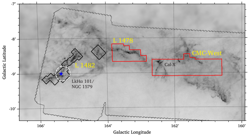
Figure 1: CO survey outlines over Herschel +Planck dust maps. The CO survey boundary is outlined in black and red, with the black outlined covering L1482, the southeastern extent of the cloud, being initially presented in K15 and the red outlines indicating the new data presented in this paper (L1478, and CMC-West). ${}^{12}\text{CO}$ and ${}^{13}\text{CO}$ were observed in all 3 regions, while $\text{C}{}^{18}\text{O}$ was not observed in CMC-West. The jagged black boarder marks the extent of the Herschel dust data (Lada et al., 2017), with Planck data used to fill in outside that. The Herschel data continues further west about $1\deg$. than shown on the map. The CO survey boarder was chosen to cover the majority of the $A_{\rm V}$ $>$3 mag dust. Two subregions of interest are shown. The dashed white circle shows the extent of the H II region (NGC 1579) associated with the star (shown in blue) LkH$\alpha$ 101. In CMC-West we show the Cal-X feature described in Imara et al. (2017).

For this paper we use observations obtained with the Arizona Radio Observatory (ARO) 10 m Heinrich-Hertz Submillimeter Telescope (SMT) and the Herschel Space Observatory.

2.1 Herschel dust opacity and temperature maps

We make use of the Herschel dust opacity and temperature maps from Lada et al. (2017). The CMC was observed in the "Auriga-California on Herschel program" (Harvey et al., 2013), with the PACS and SPIRE instruments. PACS 160 µm and SPIRE 250, 350, and 500 µm maps were convolved to the resolution of the 500 µm map ($\rm FWHM_{500\micron}=36\arcsec$). We briefly describe the data and the method we used to derive the ${\rm H}_{2}$ column density and dust temperature. In Lada et al. (2017) dust opacity ($\tau_{850}$) and dust temperature ($T_{\rm dust}$) were derived by fitting the Herschel spectral energy distribution (SED) for each pixel with a modified blackbody,

$$F_{\nu}=\tau_{850}\left(\frac{\nu}{\nu_{0}}\right)^{\beta_{d}}\frac{2h\nu^{3}}{c^{2}}\frac{1}{{\rm e}^{h\nu/kT_{\rm dust}}-1}$$

where, $\nu_{0}=353\ \text{GHz}$, the dust $\beta_{d}$ is fixed locally from Planck maps and $\tau_{850}$ (the opacity at 850 microns) and $T_{\rm dust}$ are free parameters. Here $T_{\rm dust}$ is an effective dust temperature since it averages over the temperature profile along the line-of-sight.

The conversion from $\tau_{850}$ to ${\rm H}_{2}$ column density (${\mathrm{N}[{{\rm H}_{2}}]}$) is done by comparing the Herschel $\tau_{850}$ maps to extinction maps of the CMC derived using the NICEST method (Lombardi, 2009). They found a linear relation between $\tau_{850}$ and $A_{\rm K}$ for this cloud,

$$A_{\rm K}=\gamma\,\tau_{850}+\delta,$$ (1)

where $\gamma=3593\rm\ mag$, which is similar to the value measured previously in the Orion B cloud (Lombardi et al., 2014) and Perseus (Zari et al., 2016). We convert from K-band extinction to V-band extinctions to facilitate comparisons to previous work. $A_{\rm K}$ is converted to ${\mathrm{N}[{{\rm H}_{2}}]}$ assuming an extinction law $A_{\rm K}/A_{\rm V}=0.11$ and a dust-to-gas ratio ${\mathrm{N}[{{\rm H}_{2}}]}/A_{\rm V}=9.4\times 10^{20}\,\text{cm}^{-2}\,\text{mag}^{-1}$ (Bohlin et al., 1978; Rachford et al., 2002). The final maps are degraded to $38\arcsec$ resolution for comparison to the CO data. The corresponds to 0.08 pc at distance to the CMC (450 pc, Lada et al. (2009)). The total (atomic + molecular) mass is found by integrating the total gas surface density ( $\Sigma_{gas}$) over the area of the cloud, ${\rm M}_{tot}=\int\Sigma_{gas}\,{\rm d}S,$ where $\Sigma_{gas}/A_{\rm K}=\ 183\,{\rm M}_{\odot}\,{\rm pc}^{-2}\,{\rm mag}^{-1}$ (Lombardi et al., 2006; Savage & Mathis, 1979). The total mass contained in the Herschel map is $5.52\times 10^{4}\ {\rm M_{\odot}}$, (Lada et al., 2017). Approximately 20% of the total cloud mass, $M=\rm 1.07\times 10^{4}M_{\odot}$, is covered by our CO survey, which is discussed below.

2.2 Carbon Monoxide Data

We observed the $J=2-1$ transition of ${}^{12}\text{CO}$ (230.528 GHz), ${}^{13}\text{CO}$ (220.339 GHz) and $\text{C}{}^{18}\text{O}$ (219.560 GHz) with the Heinrich Hertz Submillimeter Telescope (SMT) using a prototype ALMA band 6 dual-polarization sideband separating receiver in combination with the 0.25 MHz – 256 channel filterbank as the backend (0.25 MHz $\sim 0.32\rm\ km/s$ at 230 GHz). We used two observing setups - (1) with ${}^{12}\text{CO}$ in the upper-sideband and ${}^{13}\text{CO}$ in the lower-sideband and (2) another with ${}^{12}\text{CO}$ in the upper-sideband and $\text{C}{}^{18}\text{O}$ in the lower-sideband. This improves the signal-to-noise of the ${}^{12}\text{CO}$ data. CMC was observed over multiple days during the November 2012 - April 2013 observing season. Those segments are shown as outlines overlayed on Planck+Herschel dust map in Fig. 1. CMC West was not observed in $\text{C}{}^{18}\text{O}$. The survey boundaries were designed to cover regions with $A_{\rm V}\gtrsim 3\ {\rm mag}$ in the Lada et al. (2009) extinction maps.

We observed in ’on-the-fly’ (OTF) mode (Mangum et al., 2007) - raster scanning $10\arcmin\times 10\arcmin$ tiles at a rate of 10″ $\rm s^{-1}$, sampling spectra every 0.1 s. The raw OTF data were put onto a 10″grid using custom data reduction scripts in the GILDAS CLASS software package (Pety, 2018) and then had a linear baseline subtracted. Those reduced data were then exported as tiles into MIRIAD, where adjacent tiles were combined into a single map, with overlapping regions being combined using the rms weighted average. The final three contiguous regions are shown outlined in Fig. 1. From east-to-west they are L1482, L1478, and the West cloud.

We calibrated the intensity using periodic observations of the CO bright source W3(OH) (more details on the calibration method can be found in Bieging et al. (2010)). Since the beam and velocity resolution for each CO isotopologue are all slightly different, the maps were convolved to the resolution of the ${}^{12}\text{CO}$ map (38″) and regridded in velocity to 0.3 km/s channels to facilitate comparison. The average RMS noise per 0.3 km/s channel we achieve is 0.11 K for $\text{C}{}^{18}\text{O}$, 0.13 K for ${}^{13}\text{CO}$, and 0.11 K for ${}^{12}\text{CO}$. The average spectra for each region are shown in Fig. 2. The reduced maps are publicly available on the Harvard Dataverse (Lewis, 2020).

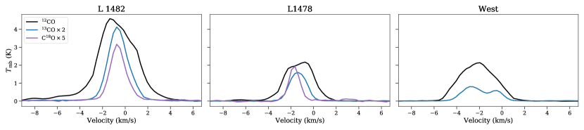
Figure 2: Average ${}^{12}\text{CO}$,${}^{13}\text{CO}$, and $\text{C}{}^{18}\text{O}$ spectra for each region of the California molecular cloud for pixels with SNR>3 for ${}^{12}\text{CO}$ and ${}^{13}\text{CO}$, and SNR>5 for $\text{C}{}^{18}\text{O}$.

3 Data Analysis

3.1 CO Moment Maps

We derived the line parameters (integrated intensity, central velocity, and velocity dispersion) using moment analysis: $M_{0}=\sum T_{\rm mb}\ {\rm\Delta v}$, $M_{1}=\frac{\sum T_{\rm mb}\,{\rm v}\ {\rm\Delta v}}{M_{0}}$, $M_{2}=\frac{\sum T_{\rm mb}\,({\rm v-}M_{1})^{2}\ {\rm\Delta v}}{M_{0}},$ where $\rm\Delta v$ is the channel width. $M_{0}$ is the integrated intensity ($W_{\mathrm{CO}}$), $M_{1}$ is the intensity weighted velocity centroid, and $\sqrt{M_{2}}$ corresponds to an intensity weighted velocity dispersion $\sigma_{\rm v}$. Moments are sensitive to noise in the spectrum, so it is important to carefully select the channels over which the integrals are performed. We use custom velocity windows for every spatial location - that is for every spectrum - in our map. Windows are created by locating the channels which contain emission in a smoothed version of the data cube. The window width and position in velocity are chosen based on the line width and line central velocity and is optimized to capture all the line emission. This method is a large improvement over using a single velocity window per isotopologue per region in the cloud. Data outside the velocity windows are masked, and moments are calculated on the masked data cube.

Moments calculated using these customized narrow windows return line parameters that are consistent with the values returned from a gaussian fit. As a test, we fit single gaussians to a set of ${}^{13}\text{CO}$ lines that were characterized by a single velocity component. We found the average difference between the velocity dispersion derived from the moment analysis and the one derived from gaussian fitting was $(\sqrt{M_{2}}-\sigma_{gauss})\sim-0.03\pm 0.07$. Similar levels of agreement are seen for ${}^{12}\text{CO}$ and $\text{C}{}^{18}\text{O}$. In general, our lines are not simple gaussians, especially for ${}^{12}\text{CO}$ emission, so gaussian fitting is not an appropriate method for deriving line parameters over the whole cloud. The results in this paper rely primarily on the $0^{\rm th}$-moment or integrated intensity so, in any event, our findings are quite insensitive to the details of setting the integration window. For our results, we only use pixel where the signal-to-noise is >3 for ${}^{12}\text{CO}$ and ${}^{13}\text{CO}$ and >5 for $\text{C}{}^{18}\text{O}$.

Maps of the integrated intensity for all three lines are shown in Appendix A for L1482, L1478, and CMC-West, the portions of the CMC that were surveyed.

3.2 Column Density

We derived column densities following the method used in K15, which we describe in Appendix B. We differ from their calculation by calculating the partition function numerically to the J=100 term rather than using an approximate form. The noise in our data limits the minimum column density we can detect to $\gtrsim 10^{14}{\rm\ cm^{-2}}$ for both isotopologues.

4 Results and Discussion

4.1 The $W_{\mathrm{CO}}$– $A_{\rm V}$ relation and $X_{\mathrm{CO}}$

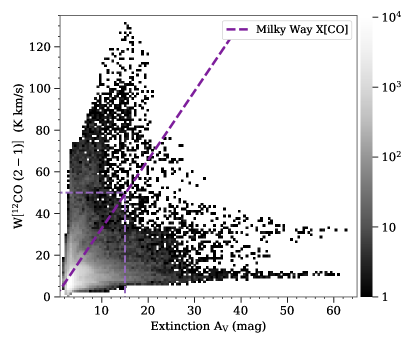
Figure 3: Binned 2D histogram for ${\mathrm{W}[{{}^{12}\text{CO}\ (2-1)}]}$ vs $A_{\rm V}$ for the entire California cloud where ${\mathrm{W}[{{}^{12}\text{CO}}]}$ is detected at greater than 3$\sigma$ ($\gtrsim 1\text{K}$). The gray dashed line is the standard relation for the adopted MW X-factor ($2\times 10^{20}$${\rm cm}^{-2}\ {(\mathrm{K\ km/s})}^{-1}$) which is 3.29 $\mathrm{K\ km/s}$$\rm\ mag^{-1}$. The blue histogram shows the number of pixels in a binned pixel of the plot on a log scale. The black dashed box shows the region containing the bulk of data range covered by previous studies (e.g., Pineda et al., 2008; Ripple et al., 2013).

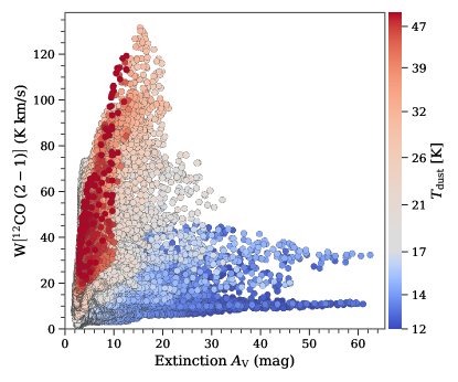
Figure 4: ${\mathrm{W}[{{}^{12}\text{CO}(2-1)}]}$ vs $A_{\rm V}$ for the entire California cloud where ${\mathrm{W}[{{}^{12}\text{CO}}]}$ is detected at greater than 3$\sigma$ ($\gtrsim 1\,\text{K}$). The points are colored by their Herschel-derived dust temperature ($T_{\rm dust}$). The points are plotted so that hotter points are plotted over cooler points.

On a plot of $W_{\mathrm{CO}}$ vs $A_{\rm V}$, a single valued X-factor is represented by a straight line through the origin. The 2-D distribution of ${\mathrm{W}[{{}^{12}\text{CO}\ (2-1)}]}$ vs $A_{\rm V}$ for the entire CMC is shown in Fig. 3. We cover a large range in extinction ($A_{\rm V}$ = 1.8 - 62.4 mag) and ${}^{12}\text{CO}$ integrated intensity ($W_{\mathrm{CO}}$ =.7 - 132 $\mathrm{K\ km/s}$). The black box shows the region of parameter space containing the bulk of the data range covered by previous studies of this relation (e.g., Pineda et al., 2008; Ripple et al., 2013). The relation corresponding to the canonical Milky Way X-factor ${\mathrm{X}[{{}^{12}\text{CO}\ (2-1)}]}_{\rm,MW}=2.9\times 10^{20}\ {\rm cm}^{-2}\ {(\mathrm{K\ km/s})}^{-1}$ is plotted for comparison. We converted the nominal $J=1-0$ CO X-factor to an X-factor for the $J=2-1$ transition by using ${\mathrm{W}[{{}^{12}\text{CO}\,(2-1)}]}$/${\mathrm{W}[{{}^{12}\text{CO}(1-0)}]}$ = 0.7 (Sakamoto et al., 1995; Yoda et al., 2010). The larger dynamic range enabled by use of the Herschel-derived extinction measurements and the increased area of the CMC included in the present survey bring the overall behavior of the W[CO]-A_V relation into sharper focus.

Confirming the earlier results of K15, it is clear from Fig. 3 that the CMC data are not well described by a single X-factor, i.e. there is no single, clear linear relationship present between ${}^{12}\text{CO}$ and $A_{\rm V}$. Typically, if there is a constant CO abundance in a molecular cloud, a linear rise of W[¹²CO] with A_V is expected at low extinctions with a break at around A_V $\approx$ 4-5 magnitudes transitioning to a flat relation at high (i.e., A_V $>$ 10 mag) extinction where the ¹²CO emission is expected to be saturated due to high line opacity and no longer sensitive to increasing dust/hydrogen column density. (e.g.; Lada et al., 1994; Lombardi et al., 2006; Pineda et al., 2008; Ripple et al., 2013; Lee et al., 2018; Glover & Clark, 2016). In the CMC the relation is considerably more complex. The plot is characterized by three branches. One branch is at low extinction and appears nearly vertical, possibly indicative of a quasi-linear relation between $W_{\mathrm{CO}}$ and $A_{\rm V}$ in that part of the diagram. At high extinctions the relation is flat and nearly horizontal, as might be expected if CO emission is saturated. However, it is separated into (at least) two distinct branches that correspond to two different levels of constant W[¹²CO], one at  10 K km/s and another at  35 K km/s.

Important clues concerning the nature of the $W_{\mathrm{CO}}$-$A_{\rm V}$ relation in the CMC are provided by Fig. 4. Here we plot the W[${}^{12}\text{CO}$ ]–$A_{\rm V}$ relation with the individual data points colored by Herschel $T_{\rm dust}$, ranging from 11.8 K - 74.4 K, plotted so cooler points are beneath hotter ones. In these plots, blue corresponds to cold dust ($T_{\rm dust}$ <18 K) and red to hotter dust ($T_{\rm dust}$ >18 K). The branches are clearly temperature dependent, with the 10 $\mathrm{K\ km/s}$  branch associated with the coldest dust, the 35 $\mathrm{K\ km/s}$  branch associated with slightly warmer dust, and the vertical branch with dust over $\sim 25\rm\ K$. The cold branches extend to low extinctions beneath the points corresponding to the hot dust in red; however 98% of the cold pixels are below 40 $\mathrm{K\ km/s}$.

Further inspection of the data shows that these branches actually correspond to different regions of the cloud. The nearly vertical branch corresponds to CO associated with hot ($T_{\rm dust}$ > 25 K) dust located in the vicinity of, and coincident with, the H II region in L1482. This is the region studied by K15 who found similar behavior in the W[CO]-Av relations with CO excitation temperature, in particular, K15 showed that the CO emission in the vicinity of the H II region is also characterized by high gas excitation temperatures. The upper horizontal branch in the figure originates in the cooler, more extended star forming regions in L1482 and from within the Cal-X region in CMC-West. The lowest ($\sim$10 $\mathrm{K\ km/s}$) horizontal branch in the Fig. 4 consists of the coldest ($T_{\rm dust}$ < 14K) material which we find to mostly originate in the L1478 and CMC-West regions of the CMC.

This complex structure is quite different from what is often seen in other clouds, where the CO emission at low extinctions (i.e., 1 $\leq$ A_V $\leq$ 3-4 magnitudes) more or less linearly increases with A_V, and then appears to flatten at higher (A_V $>$ 4 magnitudes) extinctions, though previous studies rarely extend much into the high extinctions (Frerking et al., 1982; Lada et al., 1994; Lombardi et al., 2006; Ripple et al., 2013; Kong et al., 2015; Lee et al., 2018). Indeed, none of the previous studies come close to achieving the dynamic range in cloud depth (i.e., 3 $\leq$ A_V $\leq$ 60 magnitudes) provided by the Herschel observations in our study of the CMC. These extremely deep observations, obtained on sub parsec spatial scales and across a range in cloud environments, indicate that expectations of a simple relationship between CO emission and hydrogen column density and, consequently the existence of single empirical X-factor describing all material across the cloud, may be unrealistic.

4.2 The X-factor for CO J=$2\to 1$

Table 1: Global ${}^{12}\text{CO}$ X-factor

Method	${\mathrm{X}[{{}^{12}\text{CO}\ (2-1)}]}$	K15.
$\langle{\mathrm{N}[{{\rm H}_{2}}]}/{\mathrm{W}[{{}^{12}\text{CO}}]}\rangle$	5.05 $\pm$ 1.80	4.4
$\langle{\mathrm{N}[{{\rm H}_{2}}]}\rangle/\langle{\mathrm{W}[{{}^{12}\text{CO}}]}\rangle$	4.18 $\pm$ 1.83	3.6
Linear fit through origin	2.98 $\pm$ 1.74
Average	4.1$\pm$0.8

Note. — Measurements of the global ${}^{12}\text{CO}$ (2-1) X-factor for the whole cloud in units of $10^{20}\ {\rm cm}^{-2}\ {(\mathrm{K\ km/s})}^{-1}$. The measurement methods are discussed in §4.2. The K15 are scaled by 1.4 to convert them from the original $X_{\mathrm{CO}}$ (1-0) to $X_{\mathrm{CO}}$ (2-1).

As outlined above, a single X-factor does not characterize all the gas in the cloud. We can measure the X-factor for every pixel by taking the ratio of the ${\rm H}_{2}$ column density maps and the J=2-1 CO integrated intensity maps. In the CMC, we find that ${\mathrm{X}[{{}^{12}\text{CO}\ (2-1)}]}$ ranges from $0.5-52\times 10^{20}\ {\rm cm}^{-2}\ {(\mathrm{K\ km/s})}^{-1}$. However, as previously stated, the region of the CMC that contains hot dust shows a fairly tight linear relationship between $W_{\mathrm{CO}}$ and $A_{\rm V}$, indicative of a well-defined X-factor for at least that region. Here we measure the CO X-factor for the $J=2-1$ transition, $X_{\mathrm{CO}}={\mathrm{N}[{{\rm H}_{2}}]}/{\mathrm{W}[{\rm CO\ 2-1}]}$, using three methods, where $\langle X\rangle=\frac{1}{N}\sum_{i=1}^{N}{X_{i}}$:

1. $\langle X_{\mathrm{CO}}\rangle=\langle{\mathrm{N}[{{\rm H}_{2}}]}/{\mathrm{W}[{{}^{12}\text{CO}}]}\rangle$, the average of the CO X-factor measured in each pixel, the "per-pixel" X-factor.

2. $\langle X_{\mathrm{CO}}\rangle_{\rm W}=\frac{\langle{\mathrm{N}[{{\rm H}_{2}}]}\rangle}{\langle{\mathrm{W}[{{}^{12}\text{CO}}]}\rangle}$, which is the average column density divided by the average CO integrated intensity. It is equivalent to the $W_{\mathrm{CO}}$-weighted average of the per-pixel CO X-factor, $\langle X_{\mathrm{CO}}\rangle_{W}=\frac{\sum{X_{\mathrm{CO}}W_{\mathrm{CO}}}}{\sum{W_{\mathrm{CO}}}}$.

3. $\widehat{X_{\mathrm{CO}}}$ is the solution to a least-squares linear fit through the origin to ${\mathrm{N}[{{\rm H}_{2}}]}=\widehat{X_{\mathrm{CO}}}\,W_{\mathrm{CO}}$. This is equivalent to the $(W_{\mathrm{CO}})^{2}$-weighted average of the per-pixel CO X-factor, $\widehat{}X_{\mathrm{CO}}=\frac{\sum{X_{\mathrm{CO}}W_{\mathrm{CO}}^{2}}}{\sum{W_{\mathrm{CO}}^{2}}}$

If a single X-factor existed that described the whole cloud, each method would return the same value. To estimate our uncertainty in these values we use the standard deviation for (1) and the $W_{\mathrm{CO}}$ and ($W_{\mathrm{CO}}$)² weighted standard deviation for (2) and (3) respectively. The data noise contributes negligibly being more than an order of magnitude smaller than the (weighted) standard deviation. We use the average the three methods as our accepted value and use the square-root of the average variance to derive the uncertainty. This uncertainty is a factor of $\sqrt{3}$ larger than the error derived using error propagation and better represents the variation of the X-factor in our data.

4.2.1 ${}^{12}\text{CO}$ J=2-1 X-factor

While the large scatter in the $W_{\mathrm{CO}}$–$A_{\rm V}$ relation shows that there is no single-valued X-factor that will work for all individual positions across the cloud, a globally averaged X-factor can still be computed from the data and is useful for comparison with other clouds that are either unresolved or partially resolved. Using the three methods outlined above we found results consistent with those seen in K15. The three measurements are presented in Table 1 and give an average "global X-factor" value of $(4.1\pm 0.8)\times 10^{20}\ {\rm cm}^{-2}\ {(\mathrm{K\ km/s})}^{-1}$, which is twice the Milky Way value. We next focus on the ability to measure the existence of a linear relation and measure the J=2-1 X-factor for all three isotopologues in the warm gas where all share the same $T_{\rm dust}$-dependent, nearly linear, branched structure.

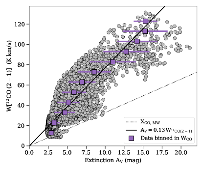
Figure 5: ${\mathrm{W}[{{}^{12}\text{CO}(2-1)}]}$ plotted against $A_{\rm V}$ for the CMC for points with $T_{\rm dust}$ > 25 K and where ${\mathrm{W}[{{}^{12}\text{CO}}]}$ is detected at greater than 3$\sigma_{W,12}$. The black dotted line is the standard adopted MW X-factor ($2\times 10^{20}$${\rm cm}^{-2}\ {(\mathrm{K\ km/s})}^{-1}$). The black solid line is the best fit solution for the data.

Table 2: J=2-1 X-factor for CO Isotopologues

Method	${\mathrm{X}[{{}^{12}\text{CO}}]}$	${\mathrm{X}[{{}^{13}\text{CO}}]}$	${\mathrm{X}[{\text{C}{}^{18}\text{O}}]}$	K15 ${}^{12}\text{CO}$
$\langle X\rangle$	1.36  (0.40)	8.99  (6.61)	59.7  (26.2)	1.8
$\langle X\rangle_{W}$	1.27  (0.36)	4.67  (3.22)	45.1  (20.8)
$\hat{X}$	1.22  (0.33)	3.55  (1.20)	36.1  (13.0)	2.1
Average	1.28 ±0.36	5.74 ±4.30	46.96 ±20.55

Note. — CO X-factor (in units of $10^{20}{\rm cm}^{-2}\ {(\mathrm{K\ km/s})}^{-1}$) derived from pixels containing hot dust ($T_{\rm dust}$ > 25 K) for the 2-1 transition of ${}^{12}\text{CO}$, ${}^{13}\text{CO}$, and $\text{C}{}^{18}\text{O}$ in units of $10^{20}\ {\rm cm}^{-2}\ {(\mathrm{K\ km/s})}^{-1}$ derived using the 3 methods we describe in §4.2. The 1$\rm\sigma$ error is in parenthesis. We adopt the average value for each isotopologue as the accepted values of the X-factor. The error is calculated as the square-root of the average variance (the variance is the square of the 1$\rm\sigma$ error). We converted converted the Kong et al. values to ${}^{12}\text{CO}$ (2-1) by scaling with $W_{2-1}/W_{1-0}=0.7$.

References. — K15

We measure the ${}^{12}\text{CO}$ J=2-1 X-factor in the region of hot ($T_{\rm dust}$ >25 K) dust where ${\mathrm{W}[{{}^{12}\text{CO}}]}$ and $A_{\rm V}$ are correlated (Pearson $r$ = 0.88) using the 3 methods described above. Those data are shown in Fig. 5 with the data binned along the $W_{\mathrm{CO}}$ axis shown in purple. The results are given in Table 4.2.1. The X-factors derived are all consistent with each other within $\sim 1\sigma$ ranging from $(1.2-1.4)\times 10^{20}\ {\rm cm}^{-2}\ {(\mathrm{K\ km/s})}^{-1}$, a little less than 1/2 the Milky Way value. Taking the average of the 3 methods as our X-factor, we find that the ${}^{12}\text{CO}$ (2-1) X-factor for $T_{\rm dust}$ > 25 K is

$$\begin{split}{\mathrm{X}[{{}^{12}\text{CO}\,(2-1)}]}&=(1.28\pm 0.36)\\ &\times 10^{20}\ {\rm cm}^{-2}\ {(\mathrm{K\ km/s})}^{-1}.\end{split}$$ (2)

It is interesting to point out here that although the ¹²CO gas in Fig. 5 is very optically thick, it exhibits the expected behavior of an optically thin tracer, i.e. $W_{\mathrm{CO}}$ increasing with dust/${\rm H}_{2}$ column density. We find no significant trends in the hot dust in $W_{\mathrm{CO}}$ with CO velocity dispersion, $\sigma_{{}^{12}\text{CO}}$, or with $T_{\rm dust}$ that would provide the increase necessary in the optically thick W[CO] to explain the linear relation in the hot dust pixels. The linear relation seems to be mostly due to a correlation between $T_{\rm peak}$ and $A_{\rm V}$ in the hot dust as was similarly found in K15. We can estimate an effective optical depth, $\tau_{\rm eff,12}$, for ${}^{12}\text{CO}$ by comparing the $X_{\mathrm{CO}}$ one would expect from an optically thin gas to the measured ${\mathrm{X}[{{}^{12}\text{CO}}]}$, $\tau_{\rm eff,12}=\ln{\left(X_{\rm obs}/X_{\rm thin}\right)}$. The optically thin CO X-factor can be found by dividing equation (B4) by ${\mathrm{N}[{{\rm H}_{2}}]}$ and assuming $\tau<<1$ to get:

$$X_{\rm thin}=C(T_{\rm ex})/[{}^{12}\text{CO}],$$ (3)

where $C(T_{\rm ex})$ is as defined in equation (B5), $[{}^{12}\text{CO}]$ is the CO:${\rm H}_{2}$ abundance ratio ${10^{-4}}$, and for $T_{\rm ex}$ we use mean excitation temperature of the hot dust pixels, $T_{\rm ex}\sim 20{\rm\ K}$. We find $X_{12,\,thin}=5.26\times 10^{18}\ {\rm cm}^{-2}\ {(\mathrm{K\ km/s})}^{-1}$ which gives $\tau_{\rm eff,12}\approx 3$. Bolatto et al. (2013) finds a similar estimate for the optically thin ${}^{12}\text{CO}$ X-factor.

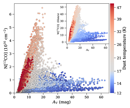
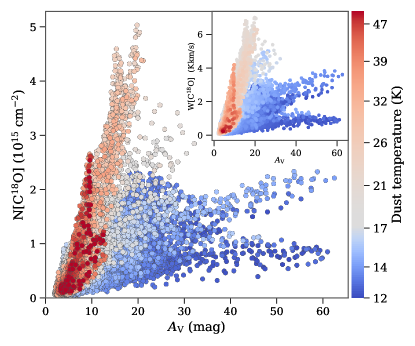
Figure 6: Plot of the (Left) ${}^{13}\text{CO}$ and (Right) $\text{C}{}^{18}\text{O}$ column density vs visual extinction colored by $T_{\rm dust}$. The colorbar shows colder pixels as blue, transitioning through gray, and becoming redder as the temperature increases. Data is plotted so that higher temperature points are plotted over cooler points to to emphasize the temperature dependent structure in the plot. The inset shows $W_{\mathrm{CO}}$ vs $A_{\rm V}$ for the line with the same coloring scheme.

4.2.2 ${}^{13}\text{CO}$ & $\text{C}{}^{18}\text{O}$ J=2-1 X-factor

We measure the X-factors for ${}^{13}\text{CO}$ and $\text{C}{}^{18}\text{O}$ for $J=2-1$ in the same way as done for ${}^{12}\text{CO}$. For both lines, $W_{\mathrm{CO}}$ is well correlated with extinction (Pearson $r>0.9$) in the hot dust, indicating the presence of a simple linear relationship with extinction. In the hot dust we find an average ${}^{13}\text{CO}$ X-factor of,

$${\mathrm{X}[{{}^{13}\text{CO}\,(2-1)}]}=(5.74\pm 4.30)\times 10^{20}\ {\rm cm}^{-2}\ {(\mathrm{K\ km/s})}^{-1},$$ (4)

and an average $\text{C}{}^{18}\text{O}$ X-factor of,

$${\mathrm{X}[{\text{C}{}^{18}\text{O}\,(2-1)}]}=(4.70\pm 2.05)\times 10^{21}\ {\rm cm}^{-2}\ {(\mathrm{K\ km/s})}^{-1}.$$ (5)

The error is large here because the linear correlation visible in the hot dust does not pass through the origin like it does for ${}^{12}\text{CO}$.

Both ${}^{13}\text{CO}$ and $\text{C}{}^{18}\text{O}$ are expected to be optically thin. Assuming a ${}^{12}\text{CO}$ abundance relative to ${\rm H}_{2}$ of 1$\times 10^{-4}$, $\rm{}^{12}C/^{13}C=69$, and $\rm{}^{16}O/^{18}O=557$ (Wilson, 1999) we can apply the same process as above to determine effective optical depths for both lines. For ${}^{13}\text{CO}$ and $\text{C}{}^{18}\text{O}$ we find $\tau_{\rm eff}$ equals 0.69 and 0.31, respectively. If, instead of using $T_{\rm ex}$ = 20 K, we use the ${}^{12}\text{CO}$ excitation temperature we derived for each pixel (see Appendix B) and compare $X_{\rm thin}(T_{\rm ex})$ (eq. 3) to $X_{\mathrm{CO}}$ in each pixel, we find that on average $\tau\approx 0$. In other words, the X-factors we measure are consistent with those predicted by an optically thin model using the ${}^{12}\text{CO}$ excitation temperature and cosmic abundance ratios.

4.3 N[CO] vs. $A_{\rm V}$

In Fig. 6 we show the ${}^{13}\text{CO}$ and $\text{C}{}^{18}\text{O}$ column density plotted against extinction with points colored by $T_{\rm dust}$. They show the same temperature dependent branched structure as ${}^{12}\text{CO}$, with $\text{C}{}^{18}\text{O}$ showing two very distinct cold branches. Plots of $W_{\mathrm{CO}}$ vs $A_{\rm V}$ for these lines are shown inset on the corresponding ${N_{\mathrm{CO}}}$ vs $A_{\rm V}$ figure. The plots of $W_{\mathrm{CO}}$–$A_{\rm V}$ for $\text{C}{}^{18}\text{O}$ and ${}^{13}\text{CO}$ are very similar to the corresponding ${N_{\mathrm{CO}}}$–$A_{\rm V}$ plots, suggesting a tight correlation between $W_{\mathrm{CO}}$ and ${N_{\mathrm{CO}}}$. For both lines, the Pearson correlation coefficient between $W_{\mathrm{CO}}$ and ${N_{\mathrm{CO}}}$ is $r>0.9$. In the optically thin limit equation B4 becomes $N_{\rm CO}=C(T_{\rm ex})W_{\rm CO}$. The best fit $T_{\rm ex}$ is 7.6 K for ${}^{13}\text{CO}$ and 9.9 K for $\text{C}{}^{18}\text{O}$, or equivalently

$${\mathrm{N}[{{}^{13}\text{CO}}]} =9.2\times 10^{14}\ {\mathrm{W}[{{}^{13}\text{CO}}]}$$ (6)

$${\mathrm{N}[{\text{C}{}^{18}\text{O}}]} =6.8\times 10^{14}\ {\mathrm{W}[{\text{C}{}^{18}\text{O}}]}.$$ (7)

This is consistent with the median $T_{\rm ex}$ derived from ${}^{12}\text{CO}$, 7.9 K for the pixels with ${}^{13}\text{CO}$ and 9.9 K for those with $\text{C}{}^{18}\text{O}$.

When deriving the column density we also derive the optical depth. In the cold branches the ${}^{13}\text{CO}$ optical depth is $\lesssim 1.5$, while $\text{C}{}^{18}\text{O}$ is optically thin ($\tau_{18}<0.75$) everywhere. With $\tau<2$, if CO is in the gas phase, we expect to see $W_{\mathrm{CO}}$ and ${N_{\mathrm{CO}}}$ increase with $A_{\rm V}$. Instead ${}^{13}\text{CO}$ shows a distinct flattening in both beyond $A_{\rm V}\sim 10$ and $\text{C}{}^{18}\text{O}$ even shows some evidence for flattening in the coldest branch (the lowest branch on the plot). The three branches are most distinct in $\text{C}{}^{18}\text{O}$, with the vertical and upper horizontal branches coming from L1482, and the lowest (and coldest, $T_{\rm dust}$ $\sim$12-13 K for $A_{\rm V}$ >30 mag) originating in L1478. The pixels that make up the upper horizontal branch, are warmer due to being associated with a region with a large number of embedded young stars.

4.3.1 The ${}^{13}\text{CO}$ and $\text{C}{}^{18}\text{O}$ Abundance

Using our CO and ${\rm H}_{2}$ column density measurements we can measure the ${}^{13}\text{CO}$:${\rm H}_{2}$ and $\text{C}{}^{18}\text{O}$:${\rm H}_{2}$ ratios, which are the abundances relative to ${\rm H}_{2}$. Square braces, $[\cdot]$, will be used to denote the abundance relative to ${\rm H}_{2}$. The abundance relative to H is simply $0.5\times$ the abundance relative to ${\rm H}_{2}$. The line-of-sight abundance can be determined by simply dividing the column density maps by the ${\mathrm{N}[{{\rm H}_{2}}]}$ map. This in situ abundance is not constant across the cloud.

We see in Fig. 6 that again, as with ${\mathrm{W}[{{}^{12}\text{CO}}]}$–$A_{\rm V}$, only the hottest dust shows a clear linear relation. To measure the true CO abundance, we must limit our measurements to the part of the cloud where CO is likely entirely in the gas phase, namely in the region containing the hot dust. We measure the total CO abundance by measuring the average abundance, $\left\langle{N_{\mathrm{CO}}}/{\mathrm{N}[{{\rm H}_{2}}]}\right\rangle$, in the hot ($T_{\rm dust}$ >25 K) dust, using pixels with signal-to-noise >3 for ${}^{13}\text{CO}$ and >5 for $\text{C}{}^{18}\text{O}$ and $T_{\rm dust}$ > 25 K, and find

$$[{}^{13}\text{CO}] =(1.31\pm.89)\times 10^{-6}$$ (8)

$$[\text{C}{}^{18}\text{O}] =(1.27\pm.59)\times 10^{-7}$$ (9)

These measurements are consistent within the errors with abundances derived from standard atomic abundances ratios assuming all the carbon is in CO: $\rm[{}^{13}\text{CO}]_{MW}=1.45\times 10^{-6}$, $\rm[\text{C}{}^{18}\text{O}]_{MW}=1.80\times 10^{-7}$. Looking at the hot pixels, we see that a straight line through the data would not intersect the origin. By performing a linear regression to the data we can determine the linear relation between CO and ${\rm H}_{2}$.

$${\mathrm{N}[{{}^{13}\text{CO}}]} =\ 3.19\times 10^{15}(A_{\rm V}-2.50)$$ (10)

$${\mathrm{N}[{\text{C}{}^{18}\text{O}}]} =\ 2.47\times 10^{14}(A_{\rm V}-3.55)$$ (11)

These equations can be combined with equations (6) and (7) to derive a linear relation for $W_{\mathrm{CO}}$–$A_{\rm V}$. The $A_{\rm V}$ offset is the extinction below which the measured ${}^{13}\text{CO}$ or $\text{C}{}^{18}\text{O}$ column density is zero. As mentioned previously, CO has been detected at lower extinctions, below $A_{\rm V}$ $\sim$ 1 mag, in both emission (e.g.; towards the Pipe (Lombardi et al., 2006) and Cygnus (Schneider et al., 2016)) and absorption (e.g.; towards O & B stars, (Burgh et al., 2007)), so this offset is not a threshold for CO formation.

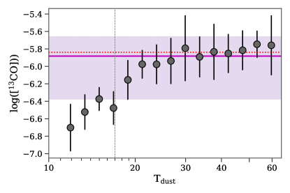
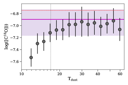
Figure 7: Binned $\log_{10}$ median abundance for (Top) ${}^{13}\text{CO}$ and (Bottom) $\text{C}{}^{18}\text{O}$ versus dust temperature. The abundance is binned by $T_{\rm dust}$ in logarithmic bins from 10 K - 63 K in 0.05 dex steps. The error-bar is the median absolute deviation scaled to the standard deviation. The purple line with the purple shaded region marks the abundance measured in the hot dust and the corresponding $1\sigma$ error. The red dashed line is the cosmic abundance

4.3.2 Abundance versus $T_{\rm dust}$

As with $W_{\mathrm{CO}}$ vs $A_{\rm V}$, ${N_{\mathrm{CO}}}$ vs $A_{\rm V}$ shows a continuous transition from the cold horizontal branches to the hot vertical branch, indicating that the abundance may be tied to the dust temperature. Plotting the bin-averaged abundance as a function of $T_{\rm dust}$ binned in 0.05 dex bins shows us that the abundance is temperature dependent. Fig. 7 shows the average CO abundance through the cloud binned by $T_{\rm dust}$ overlaid with the average abundance we derived in the hot dust with the $1\sigma$ range shown in purple and the value derived assuming cosmic abundances as a dashed red line. The abundance clearly increases with temperature and flattens out beyond $\gtrsim 20\ \text{K}$.

The ${}^{13}\text{CO}$ abundance plateaus to the abundance we measured in the hot dust, which is coincident with its cosmic abundance. $\text{C}{}^{18}\text{O}$, however, plateaus just short of its cosmic abundance. This is in part because the high temperatures span a large range in extinction, and at low extinction $\text{C}{}^{18}\text{O}$ is selectively photodissociated (K15). Because so much of the high temperature dust is at low extinction, the areas where $\text{C}{}^{18}\text{O}$ can be destroyed could dominate the average and drive the average abundance lower. This would not be much of a problem at low temperatures, since these regions are characterized by much higher $A_{\rm V}$ where the CO is better shielded from far-UV radiation. This effect is seen in photodissociation regions (PDRs), and observationally can be seen as an increase in $[{}^{13}\text{CO}]$/$[\text{C}{}^{18}\text{O}]$ or ${\mathrm{W}[{{}^{13}\text{CO}}]}$/${\mathrm{W}[{\text{C}{}^{18}\text{O}}]}$ (Shimajiri et al., 2014) and was observed in the CMC by K15. Alternatively, the difference between our measured and the cosmic $\text{C}{}^{18}\text{O}$ abundance could be caused by a variation in the $\rm{}^{18}O$ abundance. It is observed to have a large range of values, ranging from 300-600 away from the galactic center (Polehampton et al., 2005; Nittler & Gaidos, 2012), which would be enough to explain the difference we see.

The rise of abundance with $T_{\rm dust}$ is suggestive of CO desorbing from the dust grains in the warm and hot dust, with the inverse relationship being CO depletion onto grains. In Fig. 7 the transition from a positive slope to a flat one occurs around 16-20 K. This is consistent with the temperature at which CO is expected to sublimate off dust grains (Bergin et al., 1995; Bisschop et al., 2006). Bergin et al. shows that the time scale for all of the CO to desorb into the gas phase at $T_{\rm dust}$ $\sim$ 20 K is of order $100\ {\rm yrs}$. The reverse process, freeze-out or depletion, occurs at similar temperatures with timescale of $\sim 10^{6}$yrs.

In their study of the L1482, K15 suggested desorption/depletion as the cause of abundance trends with $T_{\rm ex}$. However, depletion depends on the dust temperature which they were unable to make direct comparisons too at the time. The temperatures we measure in the cold dust are significantly lower than the sublimation/depletion temperature and CO should freeze out onto grains in the cold, dense central regions of the cloud. Similar variations in the nature of the ${\mathrm{N}[{{}^{13}\text{CO}}]}$–$A_{\rm V}$ relation were found in Orion by Ripple et al. (2013) who came to the conclusion that depletion was responsible for the flattening of the relationship beyond $A_{\rm V}$ $\sim 10\ mag$.

Our observations of the relationship between CO ($W_{\mathrm{CO}}$, ${N_{\mathrm{CO}}}$) and the dust point to it being shaped by desorption/depletion processes and are consistent with previous observations of depletion (e.g.; in Orion). We conclude that the spatial variation in CO abundance in the CMC is due in large part to changes in desorption and depletion caused by the dust temperature changing with distance from star forming regions in the cloud.

5 Depletion

In this section we measure the level of depletion across the CMC and create the first maps of depletion on giant molecular cloud scales.

5.1 Measuring Depletion

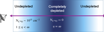
Figure 8: Schematic drawing showing how the depletion factor is an average of the depletions along the line-of-sight and necessarily underestimates the depletion in the center regions.

The depletion factor, ${\rm\eta}_{\,\text{CO}}$, is the gas phase abundance at some point in the cloud relative to the true abundance. We measure depletion independent of any outside data. We are using abundances relative to ${\rm H}_{2}$. The most similar previous study was completed by Pineda et al. (2010) in Taurus who relied on relationships between the CO and $\rm CO_{2}$ ice abundance and $A_{\rm V}$ to derive a total (gas + ice) CO column density which was used to derive a depletion factor - a method we examine later. We bypass needing to estimate the total CO column entrapped in ice by having a direct measurement of the true abundance in the hot dust (§4.3.1). We define the depletion factor the same way Kramer et al. (1999) do, as a ratio of abundances,

$${\rm\eta}_{\,\text{CO}}=\frac{A_{\rm ISM}}{A_{{\rm gas}}}=\dfrac{\left\langle{N[\text{CO}]}/{{\mathrm{N}[{{\rm H}_{2}}]}}\right\rangle_{\rm\!ISM}}{{\left({N[\text{CO}]}/{{\mathrm{N}[{{\rm H}_{2}}]}}\right)}_{{\rm\!gas}}},$$ (12)

where $A_{\rm gas}$ is the abundance in a particular pixel, and $A_{\rm ISM}$ is the true underlying abundance. We will denote depletion factors for ${}^{13}\text{CO}$ and $\text{C}{}^{18}\text{O}$ as $\eta_{13}$ and $\eta_{18}$. Hernandez et al. (2011) use a very similar method to map depletion in an infrared-dark cloud; however they derive their depletion factor relative to the CO abundance found using cosmic abundance ratios. If we were to adopt the same assumption, it would only change the result by a small multiplicative factor. The depletion factor varies from 1 (no depletion) to $\infty$ (completely depleted).

It is important to note that what we are measuring is a line-of-sight (LOS) average depletion factor, which is consequently only a lower limit to the peak depletion reached along the LOS. Fig. 8 shows a cartoon of the depletion structure of our molecular cloud. In practice any highly depleted inner region of the cloud will be measured to have a lower depletion factor than it really has due to the measurement being diluted by outer, undepleted layers of the cloud.

5.2 Depletion Factor vs $A_{\rm V}$ and $T_{\rm dust}$

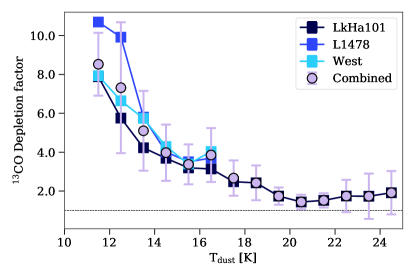
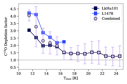
Figure 9: Depletion Trends Top: binned measurements of the ${}^{13}\text{CO}$ depletion in each California sub-region. They are binned in 1 K bins for $T_{\rm dust}$. The lines with no errors show the binned relationship for each sub-region, and the light-purple points with error-bars is the average of all the data with $1\sigma$ errorbars. The horizontal black dashed line indicates ${\rm\eta}_{\,\text{CO}}$=1. Bottom: Same as top but for $\text{C}{}^{18}\text{O}$.

Fig. 9 shows how the depletion factor varies with the dust temperature, binned in 1 K bins. The relationship for each CMC region is shown with square markers and the average for the whole cloud is shown with circles. There is a large scatter, however, the binned values show some consistency in general shape between regions, though the absolute scale can be different (e.g.; L1478 has higher measured depletion factors than L1482 in $\text{C}{}^{18}\text{O}$). The curve begins flattening out considerably between 15-18 K, and is quite flat for $T_{\rm dust}$ > 20 K. This trend is essentially the inverse of that seen in Fig. 7. The temperature range at which it transitions from a steep to flat slope, is consistent with the sublimation temperature for CO, $\sim 17\ \text{K}$.

The binned ${\rm\eta}_{\,\text{CO}}$–$T_{\rm dust}$ relationship shows a similar exponential dependence on $T_{\rm dust}$ as was noticed in Kramer et al. (1999) in $\text{C}{}^{18}\text{O}$ in the dense filament of IC 5146; however the rise seen in Kramer et al. is much shallower, having ${\rm\eta}_{\,\text{CO}}\sim 1.5$ at $T_{\rm dust}$ = 10 K. This could be due to the fact that the extinction measurements in IC 5146 covered a smaller dynamic range (1-25 magnitudes) in extinction because of the lower sensitivity of the near-infrared extinction measurements there.

5.2.1 CO on Ice

Figure 10: Plot of the total (gas + ice) $\text{C}{}^{18}\text{O}$ column density plotted against $(A_{\rm V}-3.55)$ mag. The points are colored by $T_{\rm dust}$- note that the scale is different than in Figs. 4 and 6. The red line shows the ${\mathrm{N}[{\text{C}{}^{18}\text{O}}]}$ predicted using the abundance, $[\text{C}{}^{18}\text{O}]=1.27\times 10^{-7}$ ignoring the material below the 3.55 mag threshold, ${\mathrm{N}[{\text{C}{}^{18}\text{O}}]}\propto{[\text{C}{}^{18}\text{O}]}(A_{\rm V}-3.55)$. The gray shaded region shows the $1\sigma$ uncertainty in the $\text{C}{}^{18}\text{O}$ abundance. The total column derived from adding in the contribution from ice is consistent with the total column density derived from the abundance measured in the hot dust.

Depletion results in CO being locked in ices on dust grains. The major reservoirs for CO in ice are CO ice and $\mathrm{CO}_{2}$ ice. $\mathrm{CO}_{2}$ ice is formed from the oxidation of CO on dust grains. By estimating the amount of CO locked away in ice along the LOS, we can determine the total CO column density, ${\mathrm{N}[{\rm CO}]}_{\rm total}={\mathrm{N}[{\rm CO}]}_{\rm gas}+{\mathrm{N}[{\rm CO}]}_{\rm ice}^{\rm total}$. ${\mathrm{N}[{\rm CO}]}_{\rm ice}^{\rm total}$ is the sum of the CO and CO₂ ice column densities. Using CO and $\mathrm{CO}_{2}$ spectral absorption measurements for sight-lines in Taurus with $A_{\rm V}$ between 5 - 24 mag, Whittet et al. (2007) found the following equations describing the relationship between the dust and CO and $\rm CO_{2}$ ice,

$$\rm N[{}^{12}\text{CO}]_{\rm ice} =0.400(A_{\rm V}-6.7)\times 10^{17}\ \text{cm}^{-2}\mathbf{,\ A_{\rm V}>6.7}$$

$$\rm N[{}^{12}\text{CO}_{2}]_{\rm ice} =0.252(A_{\rm V}-4.3)\times 10^{17}\ \text{cm}^{-2}\mathbf{,\ A_{\rm V}>4.3}.$$

We convert ${\mathrm{N}[{{}^{12}\text{CO}}]}_{\rm ice}^{\rm total}$ to ${\mathrm{N}[{\text{C}{}^{18}\text{O}}]}_{\rm ice}^{\rm total}$ by scaling it by the cosmic abundance ratio, $\rm{}^{16}O/^{18}O=557$. We add the ${\mathrm{N}[{\text{C}{}^{18}\text{O}}]}_{\rm ice}^{\rm total}$ to the ${\mathrm{N}[{\text{C}{}^{18}\text{O}}]}_{\rm gas}$ in pixels where $T_{\rm dust}<18{\rm\ K}$ to get ${\mathrm{N}[{\text{C}{}^{18}\text{O}}]}_{\rm total}$. In Fig. 10 we plot ${\mathrm{N}[{\text{C}{}^{18}\text{O}}]}_{\rm total}$ against $(A_{\rm V}-A_{\rm V,0})$, where $A_{\rm V,0}=3.55$ is the offset we measured for ${\mathrm{N}[{\text{C}{}^{18}\text{O}}]}$ in eqn (11). The data points are colored by the dust temperature along the same line-of-sight. ${\mathrm{N}[{\text{C}{}^{18}\text{O}}]}_{\rm total}$ shows a reasonably tight linear correlation with extinction across the entire extinction range. As a fiducial comparison we also plot in red the line that corresponds to the abundance we measured in the hot dust. The gray shaded region shows the error in the abundance. For this hot material we assume that all the CO is fully evaporated from the grains and thus that this measured abundance represents the true CO abundance in the CMC.

For $A_{\rm V}$ > 35 magnitudes the relation consists of two branches distinguished by differing dust temperatures. These branches are composed of the same pixels as those that are seen in the CO column density vs extinction plots in Fig. 6. The cold lower branch belongs to L1478 and falls along the red line consistent with the predictions derived from the Taurus ice observations. The warmer upper branch comes entirely from the extended regions around L1482. As discussed previously, L1482 has more star formation activity than the area associated with L1478. The warmer dust may indicate that there is likely less CO locked in ice in these regions than in the cold material of L1478 which is apparently well represented by the Taurus-derived relations used to predict the ice abundances. Thus application of these relations to the warm dust likely over predicts ${\mathrm{N}[{\text{C}{}^{18}\text{O}}]}_{\rm total}$ in the warmer regions. However, we note that both branches fall entirely within the shaded region of our uncertainty in the derived abundances.

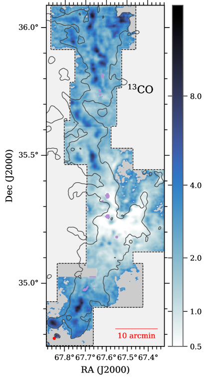
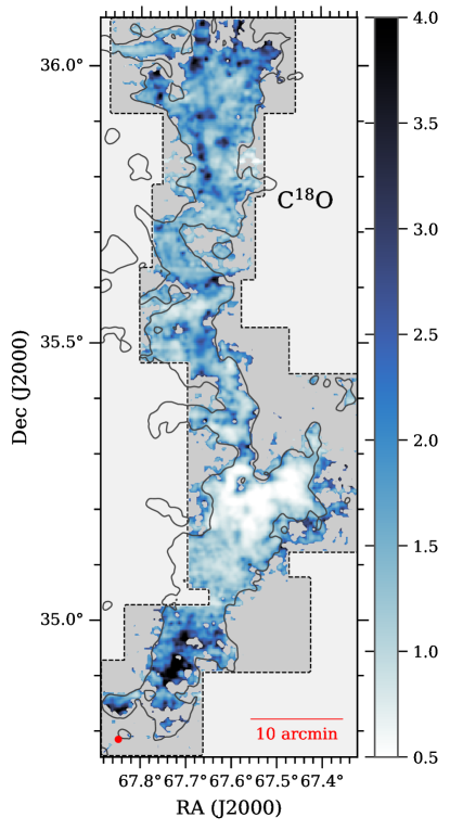
Figure 11: CO depletion maps for CMC-East (Left: ${}^{13}\text{CO}$, Right: $\text{C}{}^{18}\text{O}$). The colormap shows the highly depleted regions as dark blue, and the black contour is $A_{\rm V}$ = 5 contour. The dark gray shading marks where there was not sufficient signal-to-noise to detect emission, and the purple patches show where we were unable to calculate column densities due to the optical depth being undefined (see Appendix B). The map for $\text{C}{}^{18}\text{O}$ has been smoothed to 47.5″for display only. The black dashed line indicates the survey boundaries. The red circle shows the map resolution (${}^{13}\text{CO}$, $38\arcsec$ and $\text{C}{}^{18}\text{O}$ $47.5\arcsec$).

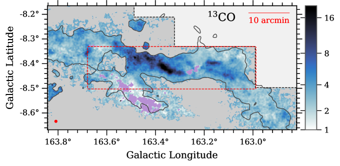
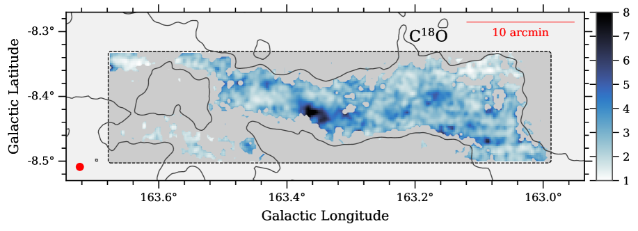
Figure 12: CO depletion maps for L1478 (Top: ${}^{13}\text{CO}$, Bottom: $\text{C}{}^{18}\text{O}$). same color scheme as Fig. 11. The red dashed box in ${}^{13}\text{CO}$ map shows boundary of the $\text{C}{}^{18}\text{O}$ survey below it.

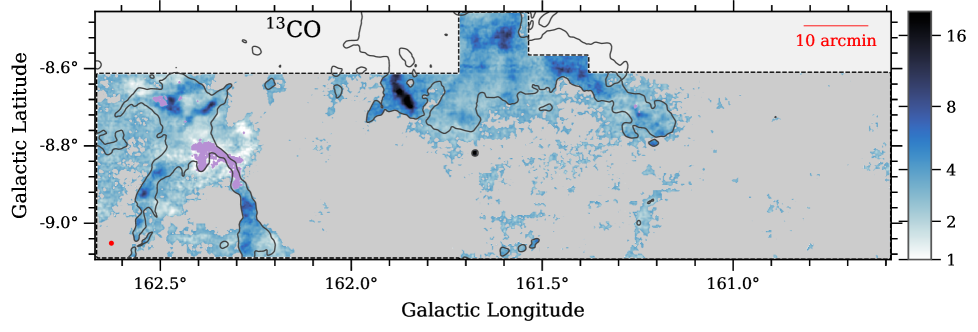
Figure 13: ${}^{13}\text{CO}$ depletion map for CMC-West. Same color scheme as Fig. 11. CMC-West was not observed in $\text{C}{}^{18}\text{O}$.

5.3 Large Scale Depletion Maps

We present the first wide-field, high resolution maps of CO depletion across a significant portion of a single GMC. In figures 11,12, & 13, we show our cloud scale maps of the ${}^{13}\text{CO}$ and $\text{C}{}^{18}\text{O}$ depletion factors, $\eta_{13}$ and $\eta_{18}$, respectively. The figures show depletion as the colormap with the $A_{\rm V}$ = 5 mag contour overlaid. The purple regions blank out places where column densities were unable to be derived due to the fact that the ${}^{13}\text{CO}$ peak intensities are larger than those of ${}^{12}\text{CO}$ (see Appendix B). The $\text{C}{}^{18}\text{O}$ depletion factor maps have been spatially smoothed (for clarity). We measure depletion factors ranging from 0.5 - 25 over the extent of the cloud. Depletion factors with values less than one arise entirely within the area coincident with the LkH$\alpha$ 101 cluster and H II region.

The maps show a great deal of spatial variation in the depletion factor. In regions where both $\text{C}{}^{18}\text{O}$ and ${}^{13}\text{CO}$ were observed, the extent of $\eta_{13}$ is greater than that of $\eta_{18}$ due to stronger ${}^{13}\text{CO}$ lines on average. $\eta_{13}$ also tends to be larger than $\eta_{18}$ (note the difference in the scale of the colorbar). Both molecules reveal clear peaks in the distribution of depletion factors across the regions. There seems to be a good general, but not perfect, correspondence between the peaks seen in the ${}^{13}\text{CO}$ and $\text{C}{}^{18}\text{O}$ depletion factors.

5.4 Depletion cores

We perform a search for cores in the depletion map using a dendrogram analysis. A good introduction to the method and its usefulness can be found in Rosolowsky et al. (2008). In short, dendrograms search for structure from the highest values down, breaking the image in to leaves (independent peaks/structures) and branches (collections of leaves and other branches) forming a tree-like representation of the structures in the data. The leaves form the list of peaks from which we select the cores. We use astrodendro (Robitaille et al., 2019) for our analysis. We identify cores only in the ${}^{13}\text{CO}$ depletion map because it has better coverage and sensitivity than the $\text{C}{}^{18}\text{O}$ depletion map. Regions with no data, or no column density measurement (i.e.; the pink regions in figures 11-13) were excluded. The input parameters for astrodendro are: min_npix=25 ($2\times$ beam area), min_delta=0.5, min_value=1, and $\rm\langle\eta_{13}\rangle$ > 2. This gave an initial list of 398 depletion peaks.

For a depletion peak to be to be identified as a core it can’t be on the map edge, at least 70% of its pixels must have $A_{\rm V}\geq 0.5\mathrm{mag}$, it must have peak $\eta_{13,peak}>3$, and $\eta_{13,peak}-\langle\eta_{13}\rangle>1$. That final criteria removes sources which don’t have a significant local peak. After this filtering 82 sources remained in our list. After examining this list we further manually removed 7 false detections. Our method is tuned to select objects we can confidently call cores and this exercise comes at the expense of a more complete sample. We identify 75 cores - 28 in the Southeast cloud which is associated with L1482, 20 in L1478, and 27 in West. Our depletion core catalog is presented in Table 3.

In Fig. 14 we show the contours for the cores overlaid on Herschel extinction, and in Appendix C we focus on each individual region and show the core’s position represented by the best fit ellipse. The best fit ellipse is found using the moment method described in Rosolowsky & Leroy (2006) which is implemented in astrodendro.

Table 3: Catalog of Depletion Cores in the California Molecular Clouds

Name	Right Ascension	Declination	Radius [pc]	$M_{\rm core}$	$T_{\rm dust}$	$A_{\rm K}$	Vcen	$\sigma_{\rm 13}$	$\sigma_{\rm 18}$	$\langle\eta_{13}\rangle$	$\langle\eta_{18}\rangle$	Zhang et al.
			pc	$M_{\odot}$	K	$\mathrm{mag}_{\rm K}$	km/s	km/s	km/s
L1482-014	4:31:04.28	35:57:40.08	0.24	30.6	14.4	0.86	-0.86	0.52	0.30	3.89	5.28	188
L1482-015	4:30:30.71	35:57:08.77	0.08	6.3	13.8	1.25	-0.97	0.59	0.32	3.56	1.80	192
L1482-016	4:30:38.33	35:58:29.51	0.07	5.9	13.5	1.53	-1.05	0.60	0.55	4.43	2.21	185
L1482-017	4:30:42.69	36:00:17.49	0.08	10.1	13.4	1.97	-1.11	0.53	0.38	6.80	3.72	183
L1482-018	4:30:15.92	36:00:15.72	0.10	13.0	13.3	1.96	-0.70	0.62	0.36	5.57	3.03	181

Note. — Abbreviated catalog of CMC depletion cores. The full catalog can be found at the end of this paper in Table 4. The radius is the beam-deconvolved radius of the source, $r_{d}$, as defined in the text. $T_{\rm dust}$ and $A_{\rm K}$ are the average Herschel dust temperature and extinction respectively. V_cen is the central velocity of the average ${}^{13}\text{CO}$ line in the core. The last column is the core number for the best-matched dust core from Zhang et al. (2018, Table 3)

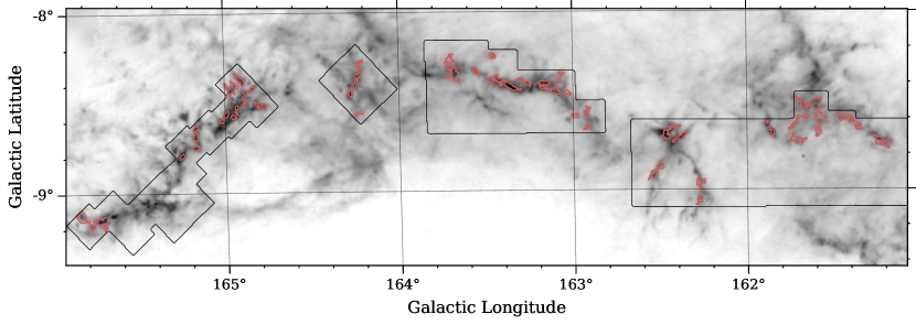
Figure 14: The core contours produced by astrodendro for our catalog of cores overlaid on the Herschel dust map in grayscale. For more detail, see the plots of each region in Appendix C

5.4.1 Core Properties

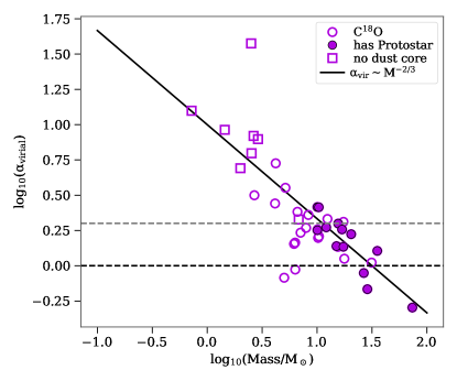
Figure 15: The log of the virial parameter, $\alpha_{\rm virial}$ plotted against log-mass for $\text{C}{}^{18}\text{O}$ depletion cores. Open and filled are are the starless and protostellar cores respectively. The squares indicate depletion cores which are not associated with a dust core in Zhang et al. (2018). The black solid line shows the $\alpha\sim M^{-2/3}$ relation from (Bertoldi & McKee, 1992) for pressure bound cores. The black dashed line is $\alpha_{\rm virial}=1$ (cores below this are virialized), and the gray dashed line is $\alpha_{\rm virial}=2$ (cores below this are bound). The $\sim 1/3$ of cores which are bound are also the most massive.

We derived a suite of properties for the cores and list them in Table 3. The core mass is defined as

$$M_{core}=\int\Sigma_{gas}\,{\rm d}S,$$

where $\Sigma_{gas}=183\,A_{\rm K}\ {\rm M_{\odot}}~{}{\rm pc}^{-2}\,\mathrm{mag}_{\rm K}^{-1}$. To account for the unrelated mass contributed by the large scale structure in the cloud, we subtract the 1 pc-scale structure from our extinction map using a python re-implementation of the FINDBACK algorithm from the CUPID package (Berry et al., 2007), and integrate over the background-subtracted map to measure the core mass. The derived masses range from 0.38 - 73 $\rm M_{\odot}$ with a mean of 10 ${\rm M_{\odot}}$. The core radius is simply $r=\sqrt{\rm Area/\pi}$, and the radius deconvolved with the telescope beam is

$$r_{d}=\sqrt{(\text{Area}/\pi)-\left({\rm FWHM}_{\rm beam}/{2}\right)^{2}}.$$

We use $r_{d}$ as the core radius for our analysis. The derived radii range from 0.04 - 0.25 pc (0.04 pc corresponds to the physical radius of a core with our minimum allowed area). From these we estimate the core number density $n=3M_{core}/(4\pi r_{d}^{3}m_{H})$. The density spans ${10^{3}}-10^{5}{\rm\ cm^{-3}}$ with $\langle\log n\rangle=4.2$. With a mean dust temperature in the cores of $\langle T_{\rm dust}\rangle\sim$ 15 K, we expect to see the onset of significant depletion (${\rm\eta}_{\,\text{CO}}$$\sim$ 5) around $n\sim 10^{4}{\rm\ cm^{-3}}$ (Bergin et al., 1995), consistent with the mean density in the cores. We also calculate the average spectrum for each core to measure the velocity dispersion using the $2^{\rm nd}$ moment of the spectrum, as described in §3.1. Since the cores are defined to be peaks in the depletion maps and most of the observed CO emission likely arises from outer undepleted layers of cloud (Fig. 8), the velocity dispersion we derive is likely an upper limit to the true velocity dispersion within the core.

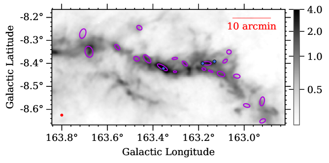
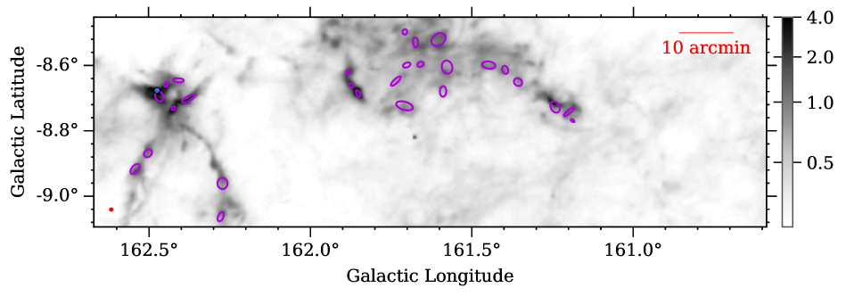
Figure 22: Map of depletion cores (ellipses) overlaid on Herschel extinction. The core’s size and locations is represented as the best fit ellipse derived using the moment method (Rosolowsky & Leroy, 2006). Protostars from Lada et al. (2017) are in blue. from The top shows L1478, and the bottom CMC-West. Our $38\arcsec$ beam is located in the lower left corner of both plots in red.

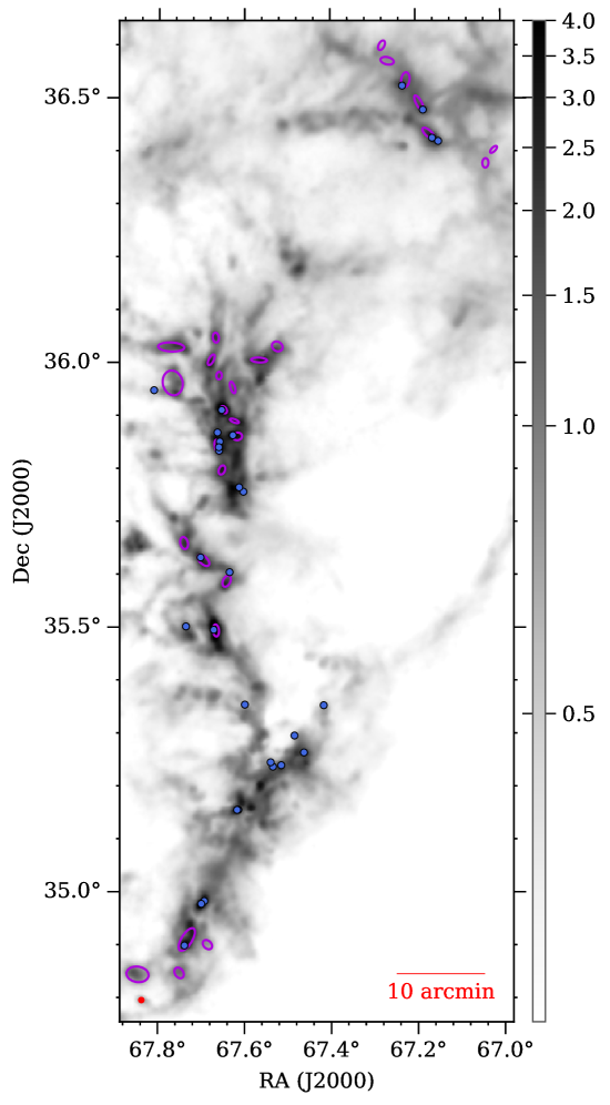
Figure 23: Same as Fig. 22 but for the L1482 region in the CMC.

We compare the position of the cores with the YSO catalog from Lada et al. (2017) , which merged Broekhoven-Fiene et al. (2014) and Harvey et al. (2013) and and updated the YSO classifications, to identify which cores contain a protostar (Class 0/I) or a disk (Class II). The protostars are shown alongside the cores in Figs. 22-23. We find that 16/75 of the cores are associated with a protostar (14) or disk (6). Several cores are associated with multiple YSOs. We consider cores with a Class 0/I source a protostellar core, and find that a large fraction of the cores are starless. The protostellar cores tend to be more massive have slightly higher densities than the starless cores, otherwise their dust temperature and size cover a fairly similar range as the starless cores considering only 20% of our cores are protostellar.

As our depletion cores are generally well correlated with extinction peaks (Figs. 14, 22-23), it is of interest to compare our depletion cores with the Herschel dust core catalog of Zhang et al. (2018). Out of 300 dust cores in that catalog, 180 are contained within our survey boundaries. We match objects in the two lists using skyellipse cross-matching in TOPCAT (Taylor, 2005) and found that roughly half (i.e., 48/75) of our depletion cores are associated with dust cores identified by Zhang et al. Only 26% (48/180) of the Zhang et al. dust cores match with our depletion cores. We list the matched dust cores in Table 3. We found that within our matched sources, the depletion core mass and radius are larger than the cross-matched dust core mass and radius. This is likely because our core identification method can produce larger cores since it tends to merge any adjacent structures that are not sufficiently higher than the background. Unmatched depletion cores are less massive and warmer than depletion cores with matches despite maintaining similar levels of measured depletion. None of the unmatched depletion cores are associated with protostars.

Some insight into the nature of the depletion cores might be gained from a virial analysis using $\text{C}{}^{18}\text{O}$ to estimate the velocity dispersion within the cores. However, because these lines arise in the outer layers of the cores (see Fig. 8), estimates of the velocity dispersions are necessarily upper limits. Nonetheless, we use $\text{C}{}^{18}\text{O}$ because it probes deeper layers of the clouds than ${}^{13}\text{CO}$ and is optically thin over the entire area it was observed. Approximately 1/2 of the ${}^{13}\text{CO}$ depletion cores have been observed in $\text{C}{}^{18}\text{O}$. We perform a simple virial analysis to examine the boundedness of these cores recognizing that the velocity dispersions we use and the virial parameters we derive are only upper limits to the true values in the depleted cores. We compute the virial parameter as

$$\alpha_{virial}\leq\frac{5\sigma^{2}r_{d}}{{\rm G}{\rm M_{core}}}$$ (13)

where $r_{d}$ is the deconvolved radius, $\rm M_{core}$ is the core mass, and $\sigma$ is the 1D velocity dispersion. The velocity dispersion $\sigma$ is the combination of the thermal and turbulent velocity dispersions, $\sigma^{2}=c_{s}^{2}+\sigma_{NT}^{2}$, where $c_{s}^{2}$ is the sound speed or thermal velocity dispersion ((Bertoldi & McKee, 1992)). Using the dust temperature as a proxy for the gas temperature, the velocity dispersion is ,

$$\sigma^{2}=\frac{kT_{\rm dust}}{\mu m_{\rm H}}+\sigma_{\rm 18}^{2}-\frac{kT_{\rm dust}}{m_{18}},$$ (14)

where $\mu=2.33$ is the mean molecular weight corrected for helium, $m_{18}$ is the mass of the $\text{C}{}^{18}\text{O}$ molecule, and $\sigma_{\rm 18}$ is the $\text{C}{}^{18}\text{O}$ velocity dispersion. Like the velocity dispersion, $T_{\rm dust}$ is also an upper limit as it includes warmer material along the line of sight. If we assumed a central core temperature of $T_{\rm dust}\sim 10{\,\rm K}$ (Roy et al. (2014) measured 9.3 K for B68), instead of using the mean dust temperature that we measure, $\sigma^{2}$ would decrease on average by $\sim$10%. We plot the $\text{C}{}^{18}\text{O}$ virial parameter against mass in Fig. 15. The filled and open symbols correspond to depletion cores with and without protostars respectively. The squares corresponds to depletion cores which do not have a match in Zhang et al.. The black dashed horizontal line is $\alpha_{\rm virial}=1$ and the gray dashed line is $\alpha_{\rm virial}=2$. Cores are virialized if $\alpha_{\rm virial}<1$ and bound for $\alpha_{\rm virial}<2$. Approximately 1/2 (23/41) of the $\text{C}{}^{18}\text{O}$ cores are gravitationally bound ($\alpha_{18}<2$) including almost all the protostellar cores. We can derive a lower limit for the virial parameter by assuming that a core’s non-thermal linewidth is $\sim$sonic towards its center. Thus the the velocity dispersion that goes into (13) is $\sigma^{2}\approx 2c_{s}^{2}$. With these assumptions, we find that all of the cores are bound with $\alpha_{\rm virial,sonic}<1$.

The black solid line in Fig. 15 shows the predicted relationship (i.e., $\alpha\sim M^{-2/3}$) between mass and $\alpha_{virial}$ for virialized clouds when the surface (i.e., external pressure) terms are included in the virial equation (Bertoldi & McKee (1992)). Similar behavior in this relation has been reported for $\text{C}{}^{18}\text{O}$ and NH₃ observations of the dense core populations in the Pipe (Lada et al. (2008), and Orion A (Kirk et al. (2017)) molecular clouds. We can infer from the behavior of the cores’ virial parameters that, even if some are not gravitationally bound, the depletion cores in the CMC are likely pressure confined. Since the virial parameter calculated here is an upper limit, it is likely that more of the cores will be shown to be bound if an undepleted species (e.g., N₂H$+$) is used to trace the very dense gas in the central regions of the cores. Future observations of additional molecular tracers (e.g., NH₃, N₂H$+$, HCN, etc.) with higher angular resolution are desirable to obtain a deeper and more complete understanding of the chemistry and kinematics of this interesting population of cores.

6 Summary & Conclusions

In this paper we investigate the relationship between molecular gas and dust over an unprecedented dynamic range of cloud depth (A_V = 3 – 60 magnitudes) within a single giant molecular cloud. We build on and significantly extend the earlier study of the California Molecular Cloud by Kong et al. (2015) by acquiring extremely deep measurements of dust extinction toward the cloud using the Herschel satellite and by enlarging, by a factor of three, the area (1 sq. deg.) of the cloud surveyed on sub-parsec spatial scales in ${}^{12}\text{CO}$, ${}^{13}\text{CO}$, and $\text{C}{}^{18}\text{O}$ J=2-1 lines using the Heinrich Hertz Submillimeter Telescope. We directly compare CO integrated intensities with extinction to derive the CO conversion or X-factors for each isotopologue across the cloud on sub-parsec spatial scales. We derive LTE ${}^{13}\text{CO}$ and $\text{C}{}^{18}\text{O}$ column densities and compare them with extinction measurements to derive the abundances of these two CO isotopologues. We compare these results to the dust temperature distribution to investigate CO depletion. We summarize our main results as follows:

1. No single ${}^{12}\text{CO}$ X-factor can describe all the gas in the cloud, confirming the earlier study of K15. We find the ${}^{12}\text{CO}$ X-factor to vary by two orders of magnitude through the cloud becoming essentially infinite at high extinctions in the regions with the coldest dust. We find the variations to be both spatially and temperature dependent.

2. Similar to K15 we find that in the hot dust ($T_{\rm dust}$ >25 K) dust we are able to measure single-valued CO 2-1 X-factors for ${}^{12}\text{CO}$, ${}^{13}\text{CO}$, and $\text{C}{}^{18}\text{O}$ that are valid to $A_{\rm V}\sim 20\ \mathrm{mag}$, well beyond the point were ${}^{12}\text{CO}$ is expected to saturate. This hot dust is confined to pixels that are coincident with the H II region associated with the LkH$\alpha$ 101 cluster and is likely heated by the exciting stars in the cluster. We assume that all the CO in this region is in the gas phase and therefore we adopt the following conversion factors for regions with undepleted CO:

   $${\rm X}_{12,2-1} =(1.28\pm 0.36)\times 10^{20}\ {\rm cm}^{-2}\ {(\mathrm{K\ km/s})}^{-1}$$

   $${\rm X}_{13,2-1} =(5.74\pm 4.30)\times 10^{20}\ {\rm cm}^{-2}\ {(\mathrm{K\ km/s})}^{-1}$$

   $${\rm X}_{18,2-1} =(4.70\pm 2.05)\times 10^{21}\ {\rm cm}^{-2}\ {(\mathrm{K\ km/s})}^{-1}$$

   In many applications it is more convenient to express the CO conversion factor with respect to cloud mass instead of column density. The corresponding values of $\alpha_{\rm CO(2-1)}$ are listed below:

   $${\rm\alpha}_{\rm 12,2-1} =2.81\ {\rm M_{\odot}}~{}{\rm pc}^{-2}(\mathrm{K\ km/s})^{-1}$$

   $${\rm\alpha}_{\rm 13,2-1} =12.6\ {\rm M_{\odot}}~{}{\rm pc}^{-2}(\mathrm{K\ km/s})^{-1}$$

   $${\rm\alpha}_{\rm 18,2-1} =103\ {\rm M_{\odot}}~{}{\rm pc}^{-2}(\mathrm{K\ km/s})^{-1}$$

   For comparison, the values of $X_{\mathrm{CO}}$ and $\alpha_{\rm CO}$ for the J=1-0 transition of ${}^{12}\text{CO}$ are $2\times 10^{20}\ {\rm cm}^{-2}\ {(\mathrm{K\ km/s})}^{-1}$ and $4.39\ {\rm M_{\odot}}~{}{\rm pc}^{-2}(\mathrm{K\ km/s})^{-1}$, respectively.

3. The ${}^{13}\text{CO}$ and $\text{C}{}^{18}\text{O}$ abundances are found to vary with dust temperature. At high dust temperatures ($T_{\rm dust}$ $\gtrsim$ 18 K) the abundance is approximately constant while for lower temperatures the abundance decreases with decreasing temperature. By 25 K all of the CO is in the gas phase, and so we measure the total CO abundance using only the pixels with $T_{\rm dust}$ > 25 K:

   $${}^{13}\text{CO}:{\rm H}_{2} =(1.31\pm.89)\times 10^{-6}$$

   $$\text{C}{}^{18}\text{O}:{\rm H}_{2} =(1.27\pm.59)\times 10^{-7}$$

   Both measurements are in reasonable agreement (within $1\sigma$) with the abundances derived from cosmic abundance ratios.

4. We conclude that the variations in gas abundances (and $X_{\mathrm{CO}}$) with dust temperature are due to depletion and desorption processes occurring in the cloud. When we correct for the expected contribution of ices to the total (ice+gas) CO column density we recover the CO gas phase column density consistent with the abundances we measure in the undepleted gas. This suggests that total (gas+ice) CO abundance in the CMC is relatively constant across the cloud.

5. Combining the CO and extinction measurements we measure depletion factors for both ${}^{13}\text{CO}$ and $\text{C}{}^{18}\text{O}$ and construct the first maps of CO depletion across the extent of an entire GMC.

6. The depletion maps show structure whose peaks we identify as depletion cores. In most cases these correspond to cores in the extinction maps, although the boundaries of the depletion cores are more clearly defined than those of the extinction cores. We produce a catalog of these cores and list their basic properties. The cores range in mass from 0.38 - 73 ${\rm M_{\odot}}$, with a characteristic mass of 10 ${\rm M_{\odot}}$. Their sizes range between 0.04 and 0.25 pc. These depletion defined cores show evidence of being pressure confined. Those that contain protostars appear to be gravitational bound.

Appendix A Integrated intensity maps

Here we show the maps of integrated intensity for ${}^{12}\text{CO}$ (2-1), ${}^{13}\text{CO}$ (2-1), and $\text{C}{}^{18}\text{O}$ (2-1) for the California Molecular Cloud. In the following maps integrated intensity is displayed as grayscale with contours. The black dashed line shows the survey boundary. $\text{C}{}^{18}\text{O}$ was only observed in L1482 and L1478 regions. We see that the integrated intensities of the various CO isotopologues show similarity in structure. In each map the beam size is shown as a red circle. We estimate the noise in our integrated intensity maps, by taking the rms of all the pixels outside the integration mask. This gives a map of noise across the observed area. The average rms scaled to the width of the largest window for each line is $0.25\ \mathrm{K\ km/s}$, $0.20\ \mathrm{K\ km/s}$, and $0.19\ \mathrm{K\ km/s}$ for ${}^{12}\text{CO}$ (2-1), ${}^{13}\text{CO}$ (2-1), and $\text{C}{}^{18}\text{O}$ (2-1) respectively.

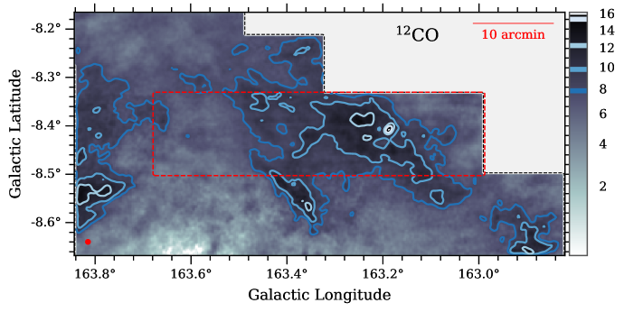
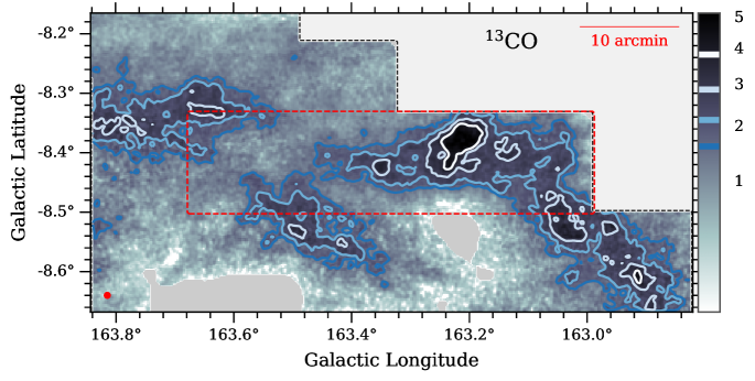
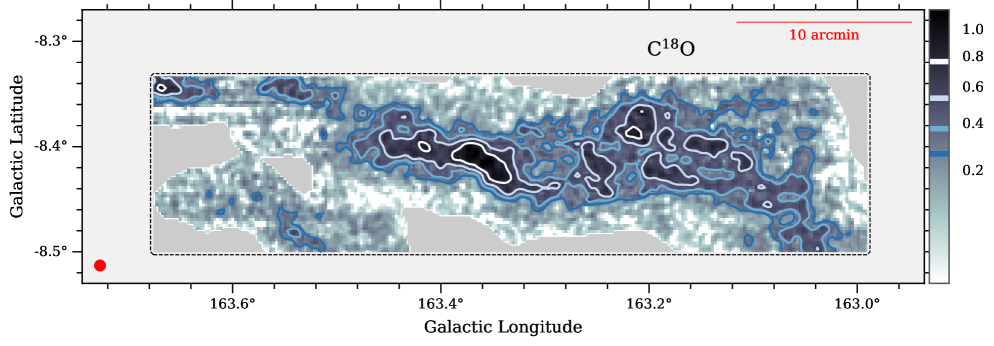
Figure 16: CO integrated intensity maps (Top:${}^{12}\text{CO}$, Middle:${}^{13}\text{CO}$, Bottom:$\text{C}{}^{18}\text{O}$) for the L1478 region in the CMC. The black dashed line indicates the survey boundaries, and the red dashed line visible in the ${}^{12}\text{CO}$ and ${}^{13}\text{CO}$ plots indicates the extent of the $\text{C}{}^{18}\text{O}$ survey. The survey resolution (38″) is shown as a red circle in the lower left hand corner. The grayscale is the total integrated intensity in K km/s. The contours from light to dark are for - ${}^{12}\text{CO}$: (6.8, 8.3, 9.6 12.0, 14.9) K km/s; ${}^{13}\text{CO}$: (1.1, 1.8, 2.5, 3.5, 5) K km/s; $\text{C}{}^{18}\text{O}$ (0.16, 0.31, 0.47, 0.74, 1.0) K km/s.

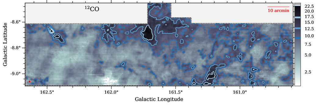
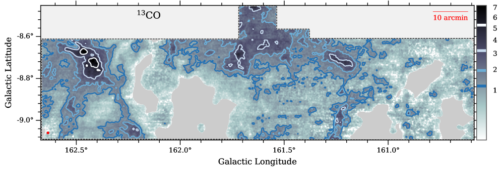
Figure 17: CO integrated intensity maps (Top:${}^{12}\text{CO}$, Bottom:${}^{13}\text{CO}$) for the West region in the CMC. The black dashed line indicates the survey boundaries. West was not observed in $\text{C}{}^{18}\text{O}$. The survey resolution (38″) is shown as a red circle in the lower left hand corner. The grayscale is the total integrated intensity in K km/s. The contours from light to dark are for - ${}^{12}\text{CO}$: (7.9, 10.1, 12.2, 17.2, 23.1) K km/s; ${}^{13}\text{CO}$: (0.8, 1.4, 2.1, 3.7, 6.8 ) K km/s.

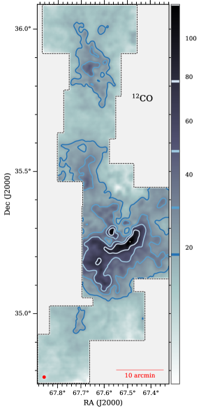
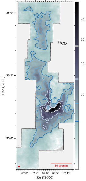
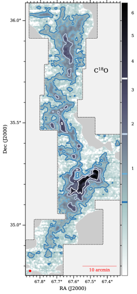
Figure 18: CO integrated intensity maps (Left:${}^{12}\text{CO}$, Middle:${}^{13}\text{CO}$, Right:$\text{C}{}^{18}\text{O}$) for the L1482 in the CMC. The black dashed line indicates the survey boundaries. The survey resolution (38″) is shown as a red circle in the lower left hand corner. The grayscale is the total integrated intensity in K km/s. The contours from light to dark are for - ${}^{12}\text{CO}$: (14.1, 21.3, 32.8, 48.5, 75.7, 112.6) K km/s; ${}^{13}\text{CO}$:(2.9, 4.9, 8.7, 13.6, 27.2, 46.1) K km/s; $\text{C}{}^{18}\text{O}$ (0.3, 0.6, 1.15, 1.7, 3.5, 5.8) K km/s.

Appendix B CO Column Density

We follow Kong et al. (2015) and Pineda et al. (2010) to calculate the total column densities of ${}^{13}\text{CO}$ and $\text{C}{}^{18}\text{O}$ assuming local thermodynamic equilibrium (LTE). In LTE, the main beam brightness temperature ($T_{\rm mb}$) is related to optical depth and excitation temperature ($T_{\rm ex}$) by

$$T_{\rm mb}=\left(\frac{h\nu/k}{e^{h\nu/kT_{\rm ex}}-1}-\frac{h\nu/k}{e^{h\nu/kT_{\rm bg}}-1}\right)(1-e^{-\tau})$$ (B1)

Under LTE, the excitation temperature can be derived from the peak temperature of an optically thick line. We use the peak main beam temperature of ${}^{12}\text{CO}$ (2-1), $T_{\rm mb,p}$, as the line is optically thick throughout California.

$$T_{\rm ex}=\frac{h\nu/k}{\ln{\!\left(1+\frac{h\nu/k}{T_{\rm mb,p}+T_{\rm bg}}\right)}}$$ (B2)

where $T_{\rm bg}=0.19~{}{\rm K}$ is the Rayleigh-Jeans equivalent temperature of the cosmic microwave background at $\nu_{{}^{12}\text{CO}(2-1)}=230.538~{}{\rm GHz}$. The excitation temperature varies from 4 - 50 K, with the distribution peaking around 7-10 K. As in K15, the highest temperatures are found in the H II region around LkH$\alpha$ 101. Additionally we find that the distribution of $T_{\rm ex}$ in L1482 is generally hotter than in L1478 and West which are far removed from the cluster and have less star formation (Lada et al., 2017). $T_{\rm ex}$ is assumed to be the same for all isotopologues. The optical depth $\tau$ of ${}^{13}\text{CO}$ (2-1) and $\text{C}{}^{18}\text{O}$ (2-1) is,

$$\tau=-\ln{\left[1-\frac{T_{\rm mb}}{h\nu/k}\left({\left(e^{\frac{h\nu}{kT_{\rm ex}}}-1\right)^{-1}-\left(e^{\frac{h\nu}{kT_{\rm bg}}}-1\right)^{-1}}\right)^{-1}\right]}.$$ (B3)

This equation is only real valued when the argument of the logarithm is positive which corresponds approximately to when the ${}^{13}\text{CO}$ or $\text{C}{}^{18}\text{O}$ brightness temperature ($T_{\rm mb}$) is less than the ${}^{12}\text{CO}$ peak brightness temperature. This is violated in some regions where ${}^{12}\text{CO}$ is self-absorbed. We mask these regions out of our analyses. Finally, the CO column density is given by,

$$N[\cdot]=C(T_{\rm ex})\times\frac{\int\tau({\rm v})\ {\rm dv}}{\int[1-e^{-\tau({\rm v})}]\ {\rm dv}}\int\!T_{\rm mb}\ {\rm dv}~{}(cm^{-2})$$ (B4)

where, $T_{\rm mb}$ is the main beam brightness temperature of ${}^{13}\text{CO}$ or $\text{C}{}^{18}\text{O}$, $\nu$ is the frequency of the transition for which we want the column density, $C(T_{\rm ex})$ is a function of the excitation temperature,

$$C(T_{\rm ex})=\frac{8\pi k\nu^{2}}{hc^{3}A_{2\rightarrow 1}}\frac{e^{\frac{h\nu}{kT_{\rm bg}}}-1}{e^{\frac{h\nu}{kT_{\rm bg}}}-e^{\frac{h\nu}{kT_{\rm ex}}}}\frac{Q}{(2J+1)e^{\frac{-hB_{0}J(J+1)}{kT_{\rm ex}}}},$$ (B5)

$$Q\equiv\sum_{J}(2J+1)e^{\frac{-hB_{0}J(J+1)}{kT_{\rm ex}}},$$

where $Q$ is the partition function which we calculate numerically to the J=100 term, at which point $Q$ has converged to within machine precision (better than 1 part in $10^{15}$) for the range of $T_{\rm ex}$ in our data, instead of using an approximation. The error associated with using the LTE approximation relative to a non-LTE determination was estimated to be a factor of $\sim 2$ in column density by K15. $\rm N_{non-LTE}/N_{LTE}$ is larger for lower column densities and is does not have a significant dependence on $T_{\rm ex}$ (Padoan et al., 2000), for ${}^{13}\text{CO}$). For the range of column densities in our data $\rm N_{non-LTE}/N_{LTE}$ ranges from $\sim 1-2$. Figs. 19, 20 and 21 show the maps of N[${}^{13}\text{CO}$ ] and N[$\text{C}{}^{18}\text{O}$ ] with areas where $\tau$ is not real-valued masked.

Figure 19: CO log(column density) maps (Top: ${}^{13}\text{CO}$, Bottom: $\text{C}{}^{18}\text{O}$) for the L1478 region in the CMC. The black dashed line indicates the survey boundaries, and the red dashed line visible in the ${}^{13}\text{CO}$ indicates the extent of the $\text{C}{}^{18}\text{O}$ survey. The survey resolution (38″) is shown as a red circle in the lower left hand corner. We mask (red with hatches) the regions of the cloud where a valid column density could not be calculated as described in Appendix B. The grayscale is the log CO column density in $\rm cm^{-2}$. The contours are - ${}^{13}\text{CO}$: (15.2, 15.5); $\text{C}{}^{18}\text{O}$ (13.5, 14.0, 14.5, 15.0)

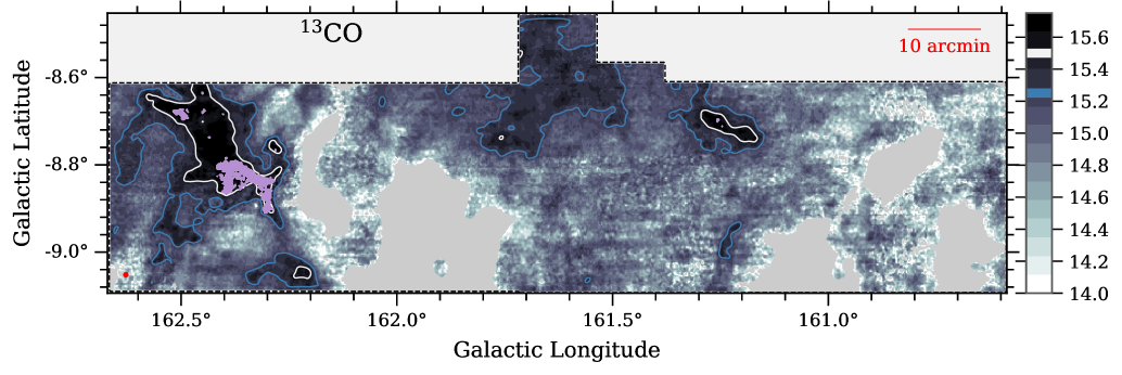
Figure 20: ${}^{13}\text{CO}$ log(column density) map for the West region in the CMC. The black dashed line indicates the survey boundaries. The survey resolution (38″) is shown as a red circle in the lower left hand corner. We mask (in the filled purple regions) the regions of the cloud where a valid column density could not be calculated as described in Appendix B. The grayscale is the log CO column density in in $\rm cm^{-2}$. The contours are (15.2, 15.5).

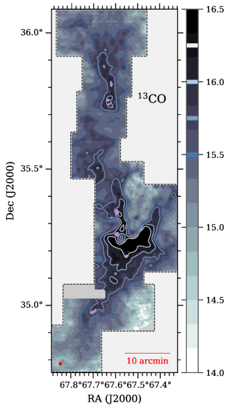
Figure 21: CO log(column density) maps (Top: ${}^{13}\text{CO}$, Bottom: $\text{C}{}^{18}\text{O}$) for the L1482 region in the CMC. The black dashed line indicates the survey boundaries, and the red dashed line visible in the ${}^{13}\text{CO}$ indicates the extent of the $\text{C}{}^{18}\text{O}$ survey. The survey resolution (38″) is shown as a red circle in the lower left hand corner.We mask (in the filled purple regions) the regions of the cloud where a valid column density could not be calculated as described in Appendix B. The grayscale is log CO column density in in $\rm cm^{-2}$. The contours from dark to light are for - ${}^{13}\text{CO}$: (15.5, 15.8, 16.0, 16.2); $\text{C}{}^{18}\text{O}$ (13.5, 14.0, 14.5, 15.0)

Appendix C ${}^{13}\text{CO}$ Depletion Core Maps

In Fig. 14, we showed the depletion core contours in the context of the entire cloud, overlaid on the Herschel extinction. Here we focus on each region and show the depletion core positions overlaid on the Herschel extinction map. We include the position of the protostars from Lada et al. (2017) in blue.

Table 4: Catalog of Depletion Cores in the California Molecular Clouds

NAME	Right Ascension	Declination	Radius [pc]	$M_{\rm core}$	$T_{\rm dust}$	$A_{\rm K}$	Vcen	$\sigma_{\rm 13}$	$\sigma_{\rm 18}$	$\langle\eta_{13}\rangle$	$\langle\eta_{18}\rangle$	Zhang et al.
			pc	$M_{\odot}$	K	$\mathrm{mag}_{\rm K}$	km/s	km/s	km/s
West-001	4:19:36.34	37:26:00.91	0.13	8.1	15.3	0.76	-0.70	0.44		5.18		103
West-002	4:19:57.06	37:30:32.60	0.19	14.9	15.4	0.71	-0.63	0.41		6.26		101
West-003	4:21:03.28	37:20:59.46	0.18	17.2	14.7	0.89	0.08	0.36		5.31		106
West-004	4:21:05.24	37:24:41.75	0.15	12.3	15.0	0.84	-0.06	0.54		4.85		104
West-005	4:16:47.84	38:24:08.92	0.05	1.3	15.7	0.62	-3.40	0.46		5.24
West-006	4:17:08.44	38:23:39.91	0.18	25.4	14.0	1.27	-3.77	0.50		4.26		13
West-007	4:16:56.39	38:24:14.09	0.08	5.3	14.2	1.04	-3.78	0.49		4.17		12
West-008	4:18:48.99	38:04:18.17	0.21	18.7	15.6	0.70	-2.23	1.04		3.79
West-009	4:21:18.31	37:33:49.77	0.06	9.3	12.1	3.25	-0.62	0.86		4.79		90
West-010	4:21:15.01	37:36:58.80	0.16	30.3	13.1	1.86	-0.65	0.85		6.15		85
West-011	4:21:35.40	37:33:29.75	0.17	49.1	13.3	2.70	-1.06	0.80		6.96		94
West-012	4:18:33.06	38:11:10.45	0.15	7.8	15.5	0.59	-2.63	0.62		4.13
West-013	4:19:27.74	37:59:51.66	0.09	20.1	12.6	3.34	-2.37	0.61		21.72		75
West-014	4:21:38.86	37:36:01.17	0.07	7.9	13.8	1.98	-1.42	0.70		5.24		87
West-015	4:19:37.54	38:00:01.09	0.06	7.5	13.2	2.40	-2.31	0.52		18.71		76
West-016	4:19:11.01	38:06:22.36	0.12	6.2	15.8	0.64	-2.43	1.16		4.15
West-017	4:17:49.60	38:22:06.79	0.14	8.4	15.1	0.67	-3.12	0.49		5.61
West-018	4:21:33.69	37:38:03.80	0.11	7.1	14.9	0.86	-1.53	0.43		4.42
West-019	4:18:46.50	38:14:51.00	0.22	23.4	15.2	0.78	-2.79	0.73		4.34		29
West-020	4:19:48.07	38:01:17.52	0.05	5.2	13.5	1.92	-2.28	0.53		11.83		73
West-021	4:18:06.23	38:22:01.59	0.13	8.0	15.0	0.79	-2.96	0.45		6.91
West-022	4:18:20.22	38:20:31.81	0.18	16.6	15.0	0.81	-3.08	0.48		6.87
West-023	4:19:14.46	38:09:52.89	0.10	4.0	15.7	0.60	-3.18	0.69		4.85
West-024	4:19:05.90	38:11:45.63	0.11	6.2	14.9	0.81	-3.00	0.65		5.04
West-025	4:19:10.45	38:17:18.70	0.26	42.3	14.2	1.07	-3.10	0.61		7.02		21
West-026	4:19:23.70	38:13:57.82	0.14	12.6	14.5	1.09	-2.95	0.59		6.07
West-027	4:19:37.65	38:13:55.32	0.08	3.3	14.8	0.73	-2.73	0.62		4.47
L1478-001	4:23:19.19	37:16:08.27	0.11	5.1	15.7	0.67	-1.28	0.57		3.63
L1478-002	4:23:48.17	37:15:57.10	0.11	4.6	15.8	0.57	-1.10	0.52		3.27
L1478-003	4:23:38.08	37:19:36.42	0.14	8.7	15.6	0.70	-1.33	0.56		3.37
L1478-004	4:24:24.86	37:19:25.83	0.12	6.1	15.6	0.63	-1.49	0.42	0.39	4.50	8.40
L1478-005	4:24:41.24	37:16:51.04	0.16	21.4	14.2	1.32	-1.58	0.53	0.31	6.44	3.82	110
L1478-006	4:25:40.50	37:07:01.95	0.19	82.6	12.8	3.65	-1.76	0.61	0.41	14.42	5.74	121
L1478-007	4:25:25.06	37:08:36.60	0.05	5.9	12.9	2.44	-1.74	0.54	0.22	10.29	5.01	120
L1478-008	4:24:53.30	37:15:24.82	0.05	3.7	13.8	1.36	-1.77	0.49	0.35	5.70	3.03	112
L1478-009	4:25:01.45	37:14:31.03	0.07	7.7	13.2	1.84	-1.92	0.50	0.29	6.27	3.30	115
L1478-010	4:25:23.86	37:11:54.88	0.11	11.3	13.6	1.42	-1.94	0.70	0.38	4.80	3.81	118
L1478-011	4:26:02.20	37:05:41.68	0.17	24.9	13.7	1.38	-1.46	0.43	0.28	10.50	4.22	122
L1478-012	4:25:04.29	37:16:05.02	0.16	32.5	13.2	2.05	-1.72	0.62	0.34	7.33	4.42	111
L1478-013	4:24:49.80	37:19:56.73	0.09	4.8	15.3	0.77	-1.37	0.51	0.36	4.09	6.53
L1478-014	4:26:11.85	37:03:41.96	0.13	11.3	14.3	1.02	-1.41	0.40	0.27	10.49	4.35
L1478-015	4:27:01.14	36:55:58.79	0.25	47.7	14.4	1.30	-1.66	0.54	0.31	4.54	7.36	131
L1478-016	4:25:37.73	37:10:58.15	0.08	3.9	14.9	0.77	-1.54	0.58	0.28	5.84	4.84
L1478-017	4:24:54.94	37:22:19.91	0.09	3.5	15.7	0.58	-1.52	0.41	0.32	3.07	3.30
L1478-018	4:26:40.09	37:02:09.39	0.12	10.6	13.9	1.22	-1.65	0.45	0.26	6.62	3.59	124
L1478-019	4:27:23.92	36:58:04.32	0.19	13.0	15.5	0.59	-1.25	0.48		4.73
L1478-020	4:26:38.82	37:09:49.67	0.12	5.5	15.4	0.62	-1.66	0.51		5.85
L1482-001	4:31:23.75	34:50:35.33	0.22	21.2	15.4	0.71	-0.68	0.37	0.28	5.30	4.55	299
L1482-002	4:31:00.11	34:50:47.39	0.11	7.7	14.8	0.92	-0.77	0.40	0.36	4.80	4.82	298
L1482-003	4:30:55.89	34:54:34.78	0.21	44.5	13.9	1.65	-0.42	0.56	0.43	5.92	5.03	296
L1482-004	4:30:44.47	34:53:59.43	0.10	5.0	15.5	0.70	-0.44	0.42	0.96	4.44	3.64
L1482-005	4:30:39.93	35:29:36.34	0.10	31.3	14.7	4.44	-0.61	0.65	0.40	5.86	2.70	232
L1482-006	4:30:33.98	35:35:11.62	0.11	13.2	15.1	1.54	-0.60	0.68	0.44	3.48	2.01	229
L1482-007	4:30:46.89	35:37:33.38	0.13	18.7	14.8	1.87	-0.87	0.61	0.36	4.28	1.75	225
L1482-008	4:30:57.75	35:39:31.13	0.12	13.4	14.1	1.55	-1.14	0.47	0.33	4.40	1.93	222
L1482-009	4:30:36.69	35:47:47.82	0.09	12.2	12.8	2.09	-1.15	0.73	0.42	5.54	3.02	210
L1482-010	4:30:39.00	35:50:26.19	0.11	23.6	13.6	2.83	-1.14	0.79	0.53	5.51	2.94	205
L1482-011	4:30:27.99	35:51:36.16	0.10	18.2	12.5	2.75	-0.79	0.77	0.54	6.02	3.05	203
L1482-012	4:30:29.72	35:53:21.97	0.06	7.5	12.8	2.68	-1.02	0.73	0.37	6.40	2.15	201
L1482-013	4:30:35.65	35:54:37.89	0.08	19.2	12.9	4.40	-1.14	0.89	0.54	7.42	3.07	197
L1482-014	4:31:04.28	35:57:40.08	0.24	30.6	14.4	0.86	-0.86	0.52	0.30	3.89	5.28	188
L1482-015	4:30:30.71	35:57:08.77	0.08	6.3	13.8	1.25	-0.97	0.59	0.32	3.56	1.80	192
L1482-016	4:30:38.33	35:58:29.51	0.07	5.9	13.5	1.53	-1.05	0.60	0.55	4.43	2.21	185
L1482-017	4:30:42.69	36:00:17.49	0.08	10.1	13.4	1.97	-1.11	0.53	0.38	6.80	3.72	183
L1482-018	4:30:15.92	36:00:15.72	0.10	13.0	13.3	1.96	-0.70	0.62	0.36	5.57	3.03	181
L1482-019	4:31:05.13	36:01:44.21	0.18	25.1	14.2	1.26	-0.68	0.88	0.41	3.73	2.15	177
L1482-020	4:30:05.72	36:01:48.07	0.12	10.3	14.6	1.13	-0.78	0.43	0.31	7.24	4.56	179
L1482-021	4:30:40.16	36:02:47.95	0.09	8.9	14.0	1.46	-1.07	0.70	0.15	7.56	3.01	176
L1482-022	4:28:08.56	36:22:36.88	0.08	3.5	15.9	0.68	0.03	0.65		6.34
L1482-023	4:28:03.94	36:24:08.44	0.06	1.8	15.8	0.56	0.07	0.73		6.17
L1482-024	4:28:40.59	36:25:58.25	0.12	16.4	13.7	1.79	-1.07	0.66	0.40	5.21	2.56	160
L1482-025	4:28:45.85	36:29:23.96	0.12	14.2	14.1	1.63	-1.07	0.53	0.35	7.35	2.61	155
L1482-026	4:28:53.39	36:32:02.45	0.13	15.4	14.5	1.43	-1.21	0.56	0.42	6.94	2.72	151
L1482-027	4:29:03.68	36:34:11.18	0.11	6.6	15.3	0.81	-1.28	1.11	0.41	5.79	2.36
L1482-028	4:29:06.82	36:35:56.29	0.07	2.2	15.4	0.64	-1.35	1.25	0.31	5.08	5.88

Note. — Catalog of CMC depletion cores. The radius is the beam-deconvolved radius of the source, $r_{d}$, as defined in the text. $T_{\rm dust}$ and $A_{\rm K}$ are the average Herschel dust temperature and extinction respectively. V_cen is the central velocity of the average ${}^{13}\text{CO}$ line in the core. The last column is the core number for the best-matched dust core from Zhang et al. (2018, Table 3)

References

- Astropy Collaboration et al. (2013) Astropy Collaboration, Robitaille, T. P., Tollerud, E. J., et al. 2013, A&A, 558, A33, doi: 10.1051/0004-6361/201322068
- Astropy Collaboration et al. (2018) Astropy Collaboration, Price-Whelan, A. M., Sipőcz, B. M., et al. 2018, AJ, 156, 123, doi: 10.3847/1538-3881/aabc4f
- Bergin et al. (1995) Bergin, E. A., Langer, W. D., & Goldsmith, P. F. 1995, ApJ, 441, 222, doi: 10.1086/175351
- Berry et al. (2007) Berry, D. S., Reinhold, K., Jenness, T., & Economou, F. 2007, in Astronomical Society of the Pacific Conference Series, Vol. 376, Astronomical Data Analysis Software and Systems XVI, ed. R. A. Shaw, F. Hill, & D. J. Bell, 425
- Bertoldi & McKee (1992) Bertoldi, F., & McKee, C. F. 1992, ApJ, 395, 140, doi: 10.1086/171638
- Bieging et al. (2010) Bieging, J. H., Peters, W. L., & Kang, M. 2010, ApJS, 191, 232, doi: 10.1088/0067-0049/191/2/232
- Bisschop et al. (2006) Bisschop, S. E., Fraser, H. J., Öberg, K. I., van Dishoeck, E. F., & Schlemmer, S. 2006, A&A, 449, 1297, doi: 10.1051/0004-6361:20054051
- Bohlin et al. (1978) Bohlin, R. C., Savage, B. D., & Drake, J. F. 1978, ApJ, 224, 132, doi: 10.1086/156357
- Bolatto et al. (2013) Bolatto, A. D., Wolfire, M., & Leroy, A. K. 2013, ARA&A, 51, 207, doi: 10.1146/annurev-astro-082812-140944
- Broekhoven-Fiene et al. (2014) Broekhoven-Fiene, H., Matthews, B. C., Harvey, P. M., et al. 2014, ApJ, 786, 37, doi: 10.1088/0004-637X/786/1/37
- Burgh et al. (2007) Burgh, E. B., France, K., & McCandliss, S. R. 2007, ApJ, 658, 446, doi: 10.1086/511259
- Frerking et al. (1982) Frerking, M. A., Langer, W. D., & Wilson, R. W. 1982, ApJ, 262, 590, doi: 10.1086/160451
- Gildas Team (2013) Gildas Team. 2013, GILDAS: Grenoble Image and Line Data Analysis Software. http://ascl.net/1305.010
- Glover & Clark (2016) Glover, S. C. O., & Clark, P. C. 2016, MNRAS, 456, 3596, doi: 10.1093/mnras/stv2863
- Harvey et al. (2013) Harvey, P. M., Fallscheer, C., Ginsburg, A., et al. 2013, ApJ, 764, 133, doi: 10.1088/0004-637X/764/2/133
- Hernandez et al. (2011) Hernandez, A. K., Tan, J. C., Caselli, P., et al. 2011, ApJ, 738, 11, doi: 10.1088/0004-637X/738/1/11
- Imara et al. (2017) Imara, N., Lada, C., Lewis, J., et al. 2017, ApJ, 840, 119, doi: 10.3847/1538-4357/aa6d74
- Kirk et al. (2017) Kirk, H., Friesen, R. K., Pineda, J. E., et al. 2017, ApJ, 846, 144, doi: 10.3847/1538-4357/aa8631
- Kong et al. (2015) Kong, S., Lada, C. J., Lada, E. A., et al. 2015, ApJ, 805, 58, doi: 10.1088/0004-637X/805/1/58
- Kramer et al. (1999) Kramer, C., Alves, J., Lada, C. J., et al. 1999, A&A, 342, 257
- Lada et al. (1994) Lada, C. J., Lada, E. A., Clemens, D. P., & Bally, J. 1994, ApJ, 429, 694, doi: 10.1086/174354
- Lada et al. (2017) Lada, C. J., Lewis, J. A., Lombardi, M., & Alves, J. 2017, A&A, 606, A100, doi: 10.1051/0004-6361/201731221
- Lada et al. (2009) Lada, C. J., Lombardi, M., & Alves, J. F. 2009, ApJ, 703, 52, doi: 10.1088/0004-637X/703/1/52
- Lada et al. (2008) Lada, C. J., Muench, A. A., Rathborne, J., Alves, J. F., & Lombardi, M. 2008, ApJ, 672, 410, doi: 10.1086/523837
- Lee et al. (2018) Lee, C., Leroy, A. K., Bolatto, A. D., et al. 2018, MNRAS, 474, 4672, doi: 10.1093/mnras/stx2760
- Lee et al. (2014) Lee, M.-Y., Stanimirović, S., Wolfire, M. G., et al. 2014, ApJ, 784, 80, doi: 10.1088/0004-637X/784/1/80
- Lewis (2020) Lewis, J. A. 2020, ARO SMT Survey of the California Molecular Cloud, V1, Harvard Dataverse, doi: 10.7910/DVN/FTOHSO
- Lombardi (2009) Lombardi, M. 2009, A&A, 493, 735, doi: 10.1051/0004-6361:200810519
- Lombardi et al. (2006) Lombardi, M., Alves, J., & Lada, C. J. 2006, A&A, 454, 781, doi: 10.1051/0004-6361:20042474
- Lombardi et al. (2014) Lombardi, M., Bouy, H., Alves, J., & Lada, C. J. 2014, A&A, 566, A45, doi: 10.1051/0004-6361/201323293
- Lynds (1962) Lynds, B. T. 1962, ApJS, 7, 1, doi: 10.1086/190072
- Mangum et al. (2007) Mangum, J. G., Emerson, D. T., & Greisen, E. W. 2007, A&A, 474, 679, doi: 10.1051/0004-6361:20077811
- Nittler & Gaidos (2012) Nittler, L. R., & Gaidos, E. 2012, Meteoritics and Planetary Science, 47, 2031, doi: 10.1111/j.1945-5100.2012.01410.x
- Padoan et al. (2000) Padoan, P., Juvela, M., Bally, J., & Nordlund, Å. 2000, ApJ, 529, 259, doi: 10.1086/308229
- Pety (2005) Pety, J. 2005, in SF2A-2005: Semaine de l’Astrophysique Francaise, ed. F. Casoli, T. Contini, J. M. Hameury, & L. Pagani, 721
- Pety (2018) Pety, J. 2018, in Submillimetre Single-dish Data Reduction and Array Combination Techniques, 11, doi: 10.5281/zenodo.1205423
- Pineda et al. (2008) Pineda, J. E., Caselli, P., & Goodman, A. A. 2008, ApJ, 679, 481, doi: 10.1086/586883
- Pineda et al. (2010) Pineda, J. L., Goldsmith, P. F., Chapman, N., et al. 2010, ApJ, 721, 686, doi: 10.1088/0004-637X/721/1/686
- Polehampton et al. (2005) Polehampton, E. T., Baluteau, J. P., & Swinyard, B. M. 2005, A&A, 437, 957, doi: 10.1051/0004-6361:20052737
- Rachford et al. (2002) Rachford, B. L., Snow, T. P., Tumlinson, J., et al. 2002, ApJ, 577, 221, doi: 10.1086/342146
- Ripple et al. (2013) Ripple, F., Heyer, M. H., Gutermuth, R., Snell, R. L., & Brunt, C. M. 2013, MNRAS, 431, 1296, doi: 10.1093/mnras/stt247
- Robitaille et al. (2019) Robitaille, T., Rice, T., Beaumont, C., et al. 2019, astrodendro: Astronomical data dendrogram creator. http://ascl.net/1907.016
- Rosolowsky & Leroy (2006) Rosolowsky, E., & Leroy, A. 2006, PASP, 118, 590, doi: 10.1086/502982
- Rosolowsky et al. (2008) Rosolowsky, E. W., Pineda, J. E., Kauffmann, J., & Goodman, A. A. 2008, ApJ, 679, 1338, doi: 10.1086/587685
- Roy et al. (2014) Roy, A., André, P., Palmeirim, P., et al. 2014, A&A, 562, A138, doi: 10.1051/0004-6361/201322236
- Sakamoto et al. (1995) Sakamoto, S., Hasegawa, T., Hayashi, M., Handa, T., & Oka, T. 1995, ApJS, 100, 125, doi: 10.1086/192210
- Sault et al. (1995) Sault, R. J., Teuben, P. J., & Wright, M. C. H. 1995, in Astronomical Society of the Pacific Conference Series, Vol. 77, Astronomical Data Analysis Software and Systems IV, ed. R. A. Shaw, H. E. Payne, & J. J. E. Hayes, 433. https://arxiv.org/abs/astro-ph/0612759
- Savage & Mathis (1979) Savage, B. D., & Mathis, J. S. 1979, ARA&A, 17, 73, doi: 10.1146/annurev.aa.17.090179.000445
- Schneider et al. (2016) Schneider, N., Bontemps, S., Motte, F., et al. 2016, A&A, 587, A74, doi: 10.1051/0004-6361/201527144
- Shimajiri et al. (2014) Shimajiri, Y., Kitamura, Y., Saito, M., et al. 2014, A&A, 564, A68, doi: 10.1051/0004-6361/201322912
- Taylor (2005) Taylor, M. B. 2005, in Astronomical Society of the Pacific Conference Series, Vol. 347, Astronomical Data Analysis Software and Systems XIV, ed. P. Shopbell, M. Britton, & R. Ebert, 29
- Whittet et al. (2007) Whittet, D. C. B., Shenoy, S. S., Bergin, E. A., et al. 2007, ApJ, 655, 332, doi: 10.1086/509772
- Wilson (1999) Wilson, T. L. 1999, Reports on Progress in Physics, 62, 143, doi: 10.1088/0034-4885/62/2/002
- Yoda et al. (2010) Yoda, T., Handa, T., Kohno, K., et al. 2010, PASJ, 62, 1277, doi: 10.1093/pasj/62.5.1277
- Zari et al. (2016) Zari, E., Lombardi, M., Alves, J., Lada, C. J., & Bouy, H. 2016, A&A, 587, A106, doi: 10.1051/0004-6361/201526597
- Zhang et al. (2018) Zhang, G.-Y., Xu, J.-L., Vasyunin, A. I., et al. 2018, A&A, 620, A163, doi: 10.1051/0004-6361/201833622