Black Hole Spin in X-ray Binaries: Giving Uncertainties an f𝑓f

Greg Salvesen CCS-2, Los Alamos National Laboratory, P.O. Box 1663, Los Alamos, NM 87545, USA. Center for Theoretical Astrophysics, Los Alamos National Laboratory, Los Alamos, NM 87545, USA. Jonah M. Miller CCS-2, Los Alamos National Laboratory, P.O. Box 1663, Los Alamos, NM 87545, USA. Center for Theoretical Astrophysics, Los Alamos National Laboratory, Los Alamos, NM 87545, USA.
(Received August 20, 2020; Revised October 08, 2020; Accepted October 15, 2020)
Abstract

The two established techniques for measuring black hole spin in X-ray binaries often yield conflicting results, which must be resolved before either method may be deemed robust. In practice, black hole spin measurements based on fitting the accretion disc continuum effectively do not marginalize over the colour correction factor fcolsubscript𝑓colf_{\mathrm{col}}. This factor parametrizes spectral hardening of the disc continuum by the disc atmosphere, whose true properties are poorly constrained. We incorporate reasonable systematic uncertainties in fcolsubscript𝑓colf_{\mathrm{col}} into the eight (non-maximal) black hole spin measurements vetted by the disc continuum fitting community. In most cases, an fcolsubscript𝑓colf_{\rm col} uncertainty of Β±plus-or-minus\pm0.2–0.3 dominates the black hole spin error budget. We go on to demonstrate that plausible departures in fcolsubscript𝑓colf_{\rm col} values from those adopted by the disc continuum fitting practitioners can bring the discrepant black hole spins into agreement with those from iron line modeling. Systematic uncertainties in fcolsubscript𝑓colf_{\rm col}, such as the effects of strong magnetization, should be better understood before dismissing their potentially dominant impact on the black hole spin error budget.

accretion, accretion discs β€” black hole physics β€” X-rays: binaries β€” X-rays: individual: LMC X–1, 4U 1543–47, GRO J1655–40, XTE J1550–564, M33 X–7, LMC X–3, H1743–322, A0620–00
††journal: Monthly Notices of the Royal Astronomical Society

1 Introduction

Black hole spin is a driver and diagnostic probe of numerous astrophysical phenomena: Relativistic jets that inject energy into their surroundings may be powered by tapping into the black hole spin energy reservoir (Penrose, 1969; Blandford & Znajek, 1977). The cosmological evolution of the coupled growth between supermassive black holes and their host galaxies is imprinted on their spin distribution (Volonteri etΒ al., 2005). Stellar mass black hole spins provide insights into core-collapse supernovae, as the natal spin is not expected to change appreciably over the lifetime of an X-ray binary system (King & Kolb, 1999). Accretion discs are also subject to interesting dynamics in the presence of a spinning black hole. When the black hole spin axis is misaligned to the accretion disc rotational axis, the disc experiences a differential precession (Lense & Thirring, 1918), which may manifest as quasi-periodic variability features (e.g., Stella & Vietri, 1998; Fragile etΒ al., 2007; Ingram etΒ al., 2009). If strong enough, this precession can cause the disc to break into distinct interacting rings of gas (Nixon etΒ al., 2012), which is one candidate mechanism for black hole state transitions (Nixon & Salvesen, 2014). Trustworthy measurements of black hole spin are necessary to realize these far-reaching astrophysical implications.

Two sophisticated techniques are at the forefront of the effort to measure black hole spin. One method is based on modeling the profile of the relativistically broadened iron emission line, which is a feature in the disc reflection spectrum (Fabian etΒ al., 1989; Laor, 1991; Miller etΒ al., 2009). The other method appeals to modeling the accretion disc continuum (Zhang etΒ al., 1997; McClintock etΒ al., 2006). In practice, the spins of supermassive black holes are only accessible with the iron line diagnostic, but both approaches can be used to measure the spins of stellar mass black holes in X-ray binaries. Cross comparing black hole spin measurements on the same set of X-ray binaries from these two independent techniques is crucial before deeming either to be robust.

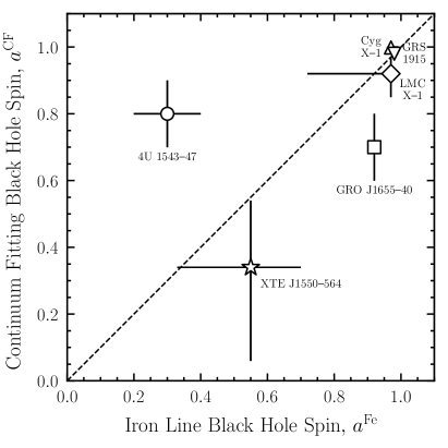
Now mature, both methods report black hole spins for a modest population of X-ray binaries (Reynolds, 2014; McClintock etΒ al., 2014). For the six systems with spins vetted by both the iron line and disc continuum fitting communities, Figure 1 shows that the techniques agree when the spin is measured to be near-maximal, but disagree otherwise. Steiner etΒ al. (2011) measured the spin of XTE J1550–564 with each technique independently, finding weak agreement as a consequence of large uncertainties. Miller etΒ al. (2009) employed both techniques simultaneously for a sample of X-ray binaries by linking the spin parameter between the disc reflection and disc continuum spectral components. While broad agreement was found with previous spin measurements from the iron line technique alone, the systems 4U 1543–47 and GRO J1655–40 showed strong discrepancies with previous disc continuum fitting results. Notably, Dong etΒ al. (2020) modeled the reflection spectrum of 4U 1543–47 and report a spin measurement consistent with that from continuum fitting. Significant discrepancy in the black hole spin obtained with two different methods for the same source is troublesome. This warrants an investigation into the validity of the assumptions behind both approaches, but in this paper we focus on disc continuum fitting.
Refer to caption
Figure 1: Black hole spin measurements from the iron line (aFesuperscriptπ‘ŽFea^{\mathrm{Fe}}) and continuum fitting (aCFsuperscriptπ‘ŽCFa^{\mathrm{CF}}) techniques plotted against one another for the sources in Table 1. Error bars are at the 68%percent6868\%-level. Spin measurements for 4U 1543–47, GRO J1655–40, and XTE J1550–564 are in disagreement, as these points do not lie on the dashed line that indicates agreement between the two techniques.

The disc continuum fitting method applies to black hole X-ray binaries in high-luminosity (LX∼0.1​LEddsimilar-tosubscript𝐿𝑋0.1subscript𝐿EddL_{X}\sim 0.1~{}L_{\rm Edd}), soft-spectral states that produce predominantly thermal emission, which is remarkably well-described by a colour-corrected, multi-temperature, blackbody model for a geometrically thin, optically thick accretion disc (e.g., Shakura & Sunyaev, 1973; GierliΕ„ski & Done, 2004). This disc continuum model approximates the local (i.e., at radius R𝑅R) specific flux as a colour-corrected blackbody

FΞ½=Ο€fcol4​Bν​(fcol​Teff),subscriptπΉπœˆπœ‹superscriptsubscript𝑓col4subscript𝐡𝜈subscript𝑓colsubscript𝑇effF_{\nu}=\frac{\pi}{f_{\rm col}^{4}}B_{\nu}\left(f_{\rm col}T_{\rm eff}\right), (1)

where BΞ½subscript𝐡𝜈B_{\nu} is the Planck function, Teffsubscript𝑇effT_{\rm eff} is the effective temperature, and fcolsubscript𝑓colf_{\rm col} is the colour correction. Local disc atmosphere models in the density and temperature regimes applicable to the high/soft state of X-ray binaries generally support this colour-corrected blackbody approximation, and its extension to a disc-integrated (i.e., continuum) model with a single fcolsubscript𝑓colf_{\rm col} value, at least for photon energies in the range ∼1similar-toabsent1\sim 1–10​keV10keV10~{}{\rm keV} (e.g., Shimura & Takahara, 1995; Davis etΒ al., 2005).

The colour-corrected, multi-temperature, disc blackbody model can be cast in terms of only two parameters (e.g., Mitsuda etΒ al., 1984), such that spectral fits directly yield a characteristic colour temperature Tcolβˆ—superscriptsubscript𝑇colβˆ—T_{\rm col}^{\ast} and the disc flux normalization Kfluxsubscript𝐾fluxK_{\rm flux}. Worked into Kfluxsubscript𝐾fluxK_{\rm flux} are the static system parameters: black hole mass M𝑀M, distance D𝐷D, inner disc inclination111The inner disc geometry can change on observational timescales in disc warping (Pringle, 1996) or disc tearing (Nixon etΒ al., 2012) scenarios, so idiscsubscript𝑖disci_{\rm disc} may not be a static parameter. idiscsubscript𝑖disci_{\rm disc}; and the dynamic parameters: inner disc radius rinsubscriptπ‘Ÿinr_{\rm in} and colour correction factor fcolsubscript𝑓colf_{\rm col}, which parametrizes spectral hardening of the disc continuum by atmospheric physics (see Appendix A). Combining independent constraints on the static parameters with knowledge of fcolsubscript𝑓colf_{\rm col}, one can convert Kfluxsubscript𝐾fluxK_{\rm flux} into a measurement of rinsubscriptπ‘Ÿinr_{\rm in}, from which the black hole spin parameter aπ‘Ža follows by assuming rinsubscriptπ‘Ÿinr_{\rm in} coincides with the location of the innermost stable circular orbit (ISCO; e.g., Zhang etΒ al., 1997). Over time, several refinements led to the modern disc continuum fitting technique discussed in Β§2, which decomposes Kfluxsubscript𝐾fluxK_{\rm flux} into its constituent parameters (e.g., McClintock etΒ al., 2006).

At the crux of measuring black hole spin from disc continuum fitting is a good estimate of fcolsubscript𝑓colf_{\rm col} for the specific observation under consideration. Physical processes operating in the disc atmosphere (e.g., electron scattering, emissive/absorptive opacities) collectively conspire to cause the observed thermal disc continuum, with characteristic colour temperature Tcolβˆ—superscriptsubscript𝑇colβˆ—T_{\rm col}^{\ast}, to be harder than that expected from a disc blackbody model with characteristic effective temperature Teffβˆ—superscriptsubscript𝑇effβˆ—T_{\rm eff}^{\ast}. In Appendix A, we describe the physics behind disc spectral hardening. The degree of spectral hardening is phenomenologically parametrized by the constant colour correction factor fcol=Tcol/Teffsubscript𝑓colsubscript𝑇colsubscript𝑇efff_{\rm col}=T_{\rm col}/T_{\rm eff} (Shimura & Takahara, 1995).222Sometimes the colour correction factor is called the spectral hardening factor and/or the symbol hdsubscriptβ„Ždh_{\rm d} or f𝑓f is used instead of fcolsubscript𝑓colf_{\rm col}.

Obtaining observational constraints on fcolsubscript𝑓colf_{\rm col} is not easy because a featureless disc continuum model can only constrain two free parameters β€” a flux amplitude and an energy shift. Notwithstanding, attempts to measure fcolsubscript𝑓colf_{\rm col} suggest it is inappropriate to draw any firm conclusions from spectral fits that blindly adopt the canonical and static value of fcol=1.7subscript𝑓col1.7f_{\rm col}=1.7 (Shimura & Takahara, 1995). Jointly fitting 26 Swift/XRT observations of the particularly clean disc component of 4U 1957+11 in the high/soft state with a relativistic thin disc model, Maitra etΒ al. (2014) obtained absolute measurements of fcolsubscript𝑓colf_{\rm col} having best-fit values of 1.9–2.1 with large 90% confidence (Β±plus-or-minus\pm) errors, typically +1.91.9+1.9 and βˆ’0.30.3-0.3. Even for a relatively unabsorbed source like 4U 1957+11, the fcolsubscript𝑓colf_{\rm col} measurements are sensitive to a strong degeneracy with the black hole spin, the presence of a high-energy Comptonization component, and the instrument bandpass (Nowak etΒ al., 2008, 2012).333Pahari etΒ al. (2018) report fcol=1.54βˆ’0.06+0.14subscript𝑓colsubscriptsuperscript1.540.140.06f_{\rm col}=1.54^{+0.14}_{-0.06} in 4U 1630–47 based on fixing M𝑀M, D𝐷D, idiscsubscript𝑖disci_{\rm disc} to their poorly constrained values with no consideration of their uncertainties.

Evidence for dynamic evolution of fcolsubscript𝑓colf_{\rm col} comes from systematic analyses of X-ray binaries over many observations and across different accretion states (e.g., Nowak etΒ al., 2008).444Belloni (2010) gives a comprehensive description of the spectral/timing state classifications of X-ray binaries. Surveying all stellar-mass black holes observed with Swift through June 2010, Reynolds & Miller (2013) studied the evolution of the disc component down to low luminosities (LX≳10βˆ’3​LEddgreater-than-or-equivalent-tosubscript𝐿𝑋superscript103subscript𝐿EddL_{X}\gtrsim 10^{-3}~{}L_{\rm Edd}) and found that rinsubscriptπ‘Ÿinr_{\rm in} increases as the source softens, if fcolsubscript𝑓colf_{\rm col} is constant. This is at odds with the disc truncation school of thought, which predicts that the inner disc radius decreases as the source transitions from the low/hard state to the high/soft state (e.g., Esin etΒ al., 1997). Supposing instead that the inner disc, which is clearly detected in the Swift data, is not severely truncated in the low/hard state, this requires fcolsubscript𝑓colf_{\rm col} to decrease as the source softens (Reynolds & Miller, 2013). Analyzing multiple state transitions of GX 339–4 observed with RXTE, Salvesen etΒ al. (2013) found that fcolsubscript𝑓colf_{\rm col} variations by factors of ∼similar-to\sim2.0–3.5 could explain the spectral evolution of the soft thermal component without invoking disc truncation.

The inability of disc continuum fitting to constrain actual values for fcolsubscript𝑓colf_{\rm col} from the data necessitates an appeal to theoretical models. As described in Β§2.2, the disc continuum fitting technique fits the data with a colour-corrected blackbody model (Li etΒ al., 2005), with each fit adopting an informed choice for fcolsubscript𝑓colf_{\rm col} based on the disc spectra predicted by a sophisticated disc atmosphere model (Davis & Hubeny, 2006). However, the reported black hole spin error budget effectively does not include systematic uncertainties associated with this choice for fcolsubscript𝑓colf_{\rm col}, which are potentially large enough to render the spin measurements moot.

We organize our paper by first introducing and re-parametrizing the disc continuum model used to measure black hole spin (Β§2; Appendix B). Next, we reverse-engineer the eight non-maximal spin measurements in Table 1 and revise them to include reasonable levels of systematic uncertainty in fcolsubscript𝑓colf_{\rm col} (Β§3.1; Appendix C). Our main result is that incorporating fcolsubscript𝑓colf_{\mathrm{col}} uncertainties at the level of Β±0.2plus-or-minus0.2\pm 0.2–0.3 dominates the black hole spin error budget (Figure 3). We go on to demonstrate that the choice for fcolsubscript𝑓colf_{\rm col} strongly influences the measured black hole spin (Β§3.2). In Β§4, we discuss the various uncertainties associated with fcolsubscript𝑓colf_{\rm col} to (i) convince the reader that the fcolsubscript𝑓colf_{\rm col} uncertainties we considered are plausible and (ii) motivate the path forward towards a better understanding of fcolsubscript𝑓colf_{\rm col} and disc atmospheric physics, with an emphasis on moderate-to-strong disc magnetization. Finally, we summarize and conclude our work in Β§5.

2 Disc Continuum Fitting Method

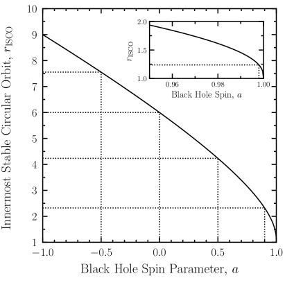
In practice, a featureless disc continuum model can only constrain two parameters when fitting an observed X-ray spectrum. The modern continuum fitting practitioners adopt the kerrbb model (Li etΒ al., 2005) and choose these two free parameters to be the mass accretion rate M˙˙𝑀\dot{M} and the black hole spin aπ‘Ža, which is equivalent to the inner disc radius rin≑Rin/Rgsubscriptπ‘Ÿinsubscript𝑅insubscript𝑅gr_{\rm in}\equiv R_{\rm in}/R_{\rm g} through its assumed association with the innermost stable circular orbit (ISCO).555The iron line technique also assumes rin=rISCOsubscriptπ‘Ÿinsubscriptπ‘ŸISCOr_{\rm in}=r_{\rm ISCO}. Figure 2 shows that the location of the ISCO is a monotonically decreasing function of the black hole spin, so measuring rin=rISCOsubscriptπ‘Ÿinsubscriptπ‘ŸISCOr_{\rm in}=r_{\rm ISCO} is tantamount to measuring aπ‘Ža. The remaining kerrbb parameters are the colour correction factor fcolsubscript𝑓colf_{\rm col}, black hole mass M𝑀M, distance D𝐷D, and inner disc inclination idiscsubscript𝑖disci_{\rm disc}, all of which are held fixed during spectral fitting.666Often, the iron line technique adopts a simpler disc model (e.g., diskbb) that can adequately fit the data without needing to specify fcolsubscript𝑓colf_{\rm col} explicitly, and so does not suffer from its uncertainty. A marginal density for aπ‘Ža is then built up by repeating this fitting procedure for many fixed sets of {fcol,M,D,idisc}subscript𝑓col𝑀𝐷subscript𝑖disc\{f_{\rm col},M,D,i_{\rm disc}\}, where M𝑀M, D𝐷D, idiscsubscript𝑖disci_{\rm disc} are sampled from their appropriate joint density (Β§2.1) and an informed choice is made for fcolsubscript𝑓colf_{\rm col} (Β§2.2).

Refer to caption
Figure 2: Radial location of the innermost stable circular orbit rISCO≑RISCO/Rgsubscriptπ‘ŸISCOsubscript𝑅ISCOsubscript𝑅gr_{\mathrm{ISCO}}\equiv R_{\mathrm{ISCO}}/R_{\mathrm{g}}, as a function of the dimensionless black hole spin parameter aπ‘Ža (Bardeen etΒ al., 1972). The inset zooms in on the region of near-maximal black hole spin, where the monotonic behaviour of rISCOsubscriptπ‘ŸISCOr_{\rm ISCO} with aπ‘Ža is very non-linear. Dotted lines mark the location of the ISCO for black hole spins: a=βˆ’0.5,0,0.5,0.9π‘Ž0.500.50.9a=-0.5,0,0.5,0.9, and 0.9980.9980.998 (inset).

As detailed in Appendix B, our approach is to recast kerrbb as a two-parameter disc model in terms of a characteristic colour temperature Tcolβˆ—superscriptsubscript𝑇colβˆ—T_{\rm col}^{\ast} and a disc flux normalization

Kfluxsubscript𝐾flux\displaystyle K_{\rm flux} ≑rin2fcol4​(G​M/c2D)2​cos⁑(idisc)absentsuperscriptsubscriptπ‘Ÿin2superscriptsubscript𝑓col4superscript𝐺𝑀superscript𝑐2𝐷2subscript𝑖disc\displaystyle\equiv\frac{r_{\rm in}^{2}}{f_{\rm col}^{4}}\left(\frac{GM/c^{2}}{D}\right)^{2}\cos\left(i_{\rm disc}\right)
Γ—Ξ₯​(idisc)​gGR​(rin,idisc)​gNT​(rin).absentΞ₯subscript𝑖discsubscript𝑔GRsubscriptπ‘Ÿinsubscript𝑖discsubscript𝑔NTsubscriptπ‘Ÿin\displaystyle\times\Upsilon\left(i_{\rm disc}\right)g_{\rm GR}\left(r_{\rm in},i_{\rm disc}\right)g_{\rm NT}\left(r_{\rm in}\right). (2)

The cornerstone of our analysis is Kfluxsubscript𝐾fluxK_{\rm flux}, while Tcolβˆ—superscriptsubscript𝑇colβˆ—T_{\rm col}^{\ast} is inconsequential.777That is, deriving rinsubscriptπ‘Ÿinr_{\rm in} from Tcolβˆ—superscriptsubscript𝑇colβˆ—T_{\rm col}^{\ast} would require knowledge of M˙˙𝑀\dot{M} (see equation B7), which is a dynamic parameter that cannot be independently determined, unlike the parameters {fcol,M,D,idisc}subscript𝑓col𝑀𝐷subscript𝑖disc\{f_{\rm col},M,D,i_{\rm disc}\} needed to derive rinsubscriptπ‘Ÿinr_{\rm in} from Kfluxsubscript𝐾fluxK_{\rm flux}. In addition to explicit dependencies on {rin,fcol,M,D,idisc}subscriptπ‘Ÿinsubscript𝑓col𝑀𝐷subscript𝑖disc\{r_{\rm in},f_{\rm col},M,D,i_{\rm disc}\}, Kfluxsubscript𝐾fluxK_{\rm flux} incorporates a limb-darkening law Ξ₯Ξ₯\Upsilon on the emitted intensity and two disc flux correction factors: gGRsubscript𝑔GRg_{\rm GR} and gNTsubscript𝑔NTg_{\rm NT}, which account for relativistic effects on photon propagation and on the radial disc structure, respectively. Following the early disc continuum fitting modelers (e.g., Sobczak etΒ al., 1999), we treat Kfluxsubscript𝐾fluxK_{\rm flux} as the observable and rinsubscriptπ‘Ÿinr_{\rm in} as the derived variable. Importantly, we define Kfluxsubscript𝐾fluxK_{\rm flux} in a way that is consistent with the kerrbb model used by the modern disc continuum fitting technique.

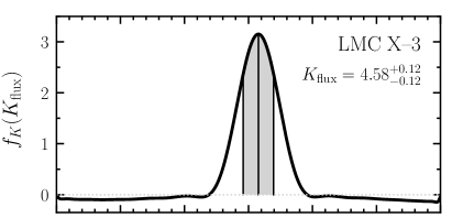
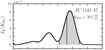
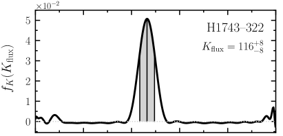
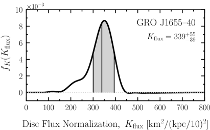
To be clear, in our subsequent analysis we do not perform any spectral fits to the disc continuum. Instead, we manipulate probability densities to reverse-engineer a published black hole spin marginal density faCF​(a)superscriptsubscriptπ‘“π‘ŽCFπ‘Žf_{a}^{\rm CF}(a) to obtain the disc flux normalization marginal density fK​(Kflux)subscript𝑓𝐾subscript𝐾fluxf_{K}(K_{\rm flux}), which is the observable in our re-parametrized continuum fitting method. With fK​(Kflux)subscript𝑓𝐾subscript𝐾fluxf_{K}(K_{\rm flux}) in hand, we can then explore how the choice for fcolsubscript𝑓colf_{\rm col} and its uncertainty affects the measured black hole spin. The actual disc continuum fitting method appeals to spectral fitting, which possesses constraining power to favor or disfavor different combinations of model parameters. Our approach allows us to explore how choosing different model parameters affects the measured black hole spin, but we cannot speak to whether these choices are in tension with the data.

Just as we took care to re-parametrize the disc continuum model in a way that is consistent with kerrbb, we must also handle the fixed kerrbb parameters {fcol,M,D,idisc}subscript𝑓col𝑀𝐷subscript𝑖disc\{f_{\rm col},M,D,i_{\rm disc}\} in a way that is consistent with the modern continuum fitting technique, as described next.

2.1 Black Hole Mass, Distance, Inner Disc Inclination

For the black hole X-ray binaries in Table 1, good independent observational constraints exist for the black hole mass M𝑀M and distance D𝐷D, but the continuum fitting practitioners equate the inner disc inclination idiscsubscript𝑖disci_{\rm disc} to the measured inclination of either the binary orbital axis iorbsubscript𝑖orbi_{\rm orb} or the jet axis ijetsubscript𝑖jeti_{\rm jet}, which is a controversial assumption (see Table 1 of Salvesen & Pokawanvit, 2020). Most continuum fitting spin measurements assume M𝑀M, D𝐷D, idiscsubscript𝑖disci_{\rm disc} to be normally and independently distributed, the latter meaning that their joint density can be decomposed into the product of their marginals,

fM,D,i​(M,D,idisc)=fM​(M)​fD​(D)​fi​(idisc).subscript𝑓𝑀𝐷𝑖𝑀𝐷subscript𝑖discsubscript𝑓𝑀𝑀subscript𝑓𝐷𝐷subscript𝑓𝑖subscript𝑖discf_{M,D,i}\left(M,D,i_{\rm disc}\right)=f_{M}\left(M\right)f_{D}\left(D\right)f_{i}\left(i_{\rm disc}\right). (3)

Of the systems in Table 1, only GRS 1915+105 (McClintock etΒ al., 2006) and Cygnus X–1 (Gou etΒ al., 2011) did not assume M𝑀M, D𝐷D, idiscsubscript𝑖disci_{\rm disc} independence. Calculating the appropriate joint density in this case is straightforward, but not necessary because we do not include GRS 1915+105 or Cygnus X–1 in our analysis for reasons explained in Β§3.

In a few cases, the marginal densities used to construct fM,D,i​(M,D,idisc)subscript𝑓𝑀𝐷𝑖𝑀𝐷subscript𝑖discf_{M,D,i}(M,D,i_{\rm disc}) were not taken to be normally distributed. For XTE J1550–564, Steiner etΒ al. (2011) adopted an asymmetric Gaussian for the distance marginal density fD​(D)subscript𝑓𝐷𝐷f_{D}(D). For H1743–322, Steiner etΒ al. (2012a) modeled the jet to derive marginal densities for the distance fD​(D)subscript𝑓𝐷𝐷f_{D}(D) and the jet / inner disc inclination fi​(idisc)subscript𝑓𝑖subscript𝑖discf_{i}(i_{\rm disc}), and they adopted a mass marginal density fM​(M)subscript𝑓𝑀𝑀f_{M}(M) based on Galactic stellar mass black hole populations.

When constructing fM,D,i​(M,D,idisc)subscript𝑓𝑀𝐷𝑖𝑀𝐷subscript𝑖discf_{M,D,i}(M,D,i_{\rm disc}) for each system in Table 1, we always use the same marginal densities and assumptions about parameter correlations / independence as the disc continuum fitting practitioners who performed the analysis for that system.

2.2 Colour Correction Factor

Good observational constraints do not exist for fcolsubscript𝑓colf_{\rm col}, so fitting a disc continuum with a colour-corrected disc model like kerrbb necessarily relies on selecting a theoretically-motivated fcolsubscript𝑓colf_{\rm col} value. To this end, the modern continuum fitting technique appeals to the bhspec model, which is based on calculations of the local emergent spectrum from a one-dimensional slab with non-local thermodynamic equilibrium radiative transfer, including the effects of thermal Compton scattering and free-free/bound-free opacities of abundant ion species (Davis etΒ al., 2005; Davis & Hubeny, 2006). Construction of bhspec involved partitioning the same relativistic global β€œΞ±π›Ό\alpha-disc” model used by kerrbb into many axisymmetric radial zones, self-consistently computing the local vertical structure and radiative transfer in each radial zone, and then integrating over all annuli to calculate the observed disc spectrum β€” accounting for relativistic photon transfer without returning radiation.

For fixed M𝑀M, D𝐷D, idiscsubscript𝑖disci_{\rm disc} and an assumed effective viscosity parameter α𝛼\alpha, bhspec has only two model parameters: the black hole spin aπ‘Ža and the Eddington-scaled disc luminosity l≑Ldisc/LEdd𝑙subscript𝐿discsubscript𝐿Eddl\equiv L_{\rm disc}/L_{\rm Edd}, which is interchangeable with mass accretion rate M˙˙𝑀\dot{M},888By defining m˙≑MΛ™/MΛ™EddΛ™π‘šΛ™π‘€subscript˙𝑀Edd\dot{m}\equiv\dot{M}/\dot{M}_{\rm Edd}, where MΛ™Edd=LEdd/(η​c2)subscript˙𝑀Eddsubscript𝐿Eddπœ‚superscript𝑐2\dot{M}_{\rm Edd}=L_{\rm Edd}/(\eta c^{2}), LEdd=4​π​G​M​mp​c/ΟƒTsubscript𝐿Edd4πœ‹πΊπ‘€subscriptπ‘šp𝑐subscript𝜎TL_{\rm Edd}=4\pi GMm_{\rm p}c/\sigma_{\rm T}, and Ldisc=η​M˙​c2subscript𝐿discπœ‚Λ™π‘€superscript𝑐2L_{\rm disc}=\eta\dot{M}c^{2}, the equivalence l=mΛ™π‘™Λ™π‘šl=\dot{m} is apparent (see also Β§4.1). whereas kerrbb requires fcolsubscript𝑓colf_{\rm col} as a third model parameter. Despite this extra parameter, the continuum fitting practitioners elect to fit the data using kerrbb because bhspec does not include returning radiation (e.g., McClintock etΒ al., 2014). Plus, bhspec sometimes gives worse fits than kerrbb despite being a more sophisticated model that dispenses with the phenomenological fcolsubscript𝑓colf_{\rm col} (e.g., Kubota etΒ al., 2010).

To take advantage of bhspec, the modern disc continuum fitting practitioners constructed the hybrid model kerrbb2 to obtain an informed fcolsubscript𝑓colf_{\rm col} for each spectral fit, as follows (e.g., McClintock etΒ al., 2006, 2010). Holding the sampled values {M,D,idisc}𝑀𝐷subscript𝑖disc\{M,D,i_{\rm disc}\} from the joint density fM,D,i​(M,D,idisc)subscript𝑓𝑀𝐷𝑖𝑀𝐷subscript𝑖discf_{M,D,i}(M,D,i_{\rm disc}) fixed, one tabulates fcolsubscript𝑓colf_{\rm col} on an (l,a)π‘™π‘Ž(l,a)-grid by fitting the colour-corrected kerrbb model to the bhspec disc atmosphere model. When tabulating fcolsubscript𝑓colf_{\rm col}, care is taken to use the same detector response matrix and energy range that will be used to fit the actual data with kerrbb.999Also, kerrbb’s rflag is turned off when fitting bhspec models, which do not include returning radiation. It is unclear if interstellar absorption is accounted for when tabulating fcolsubscript𝑓colf_{\rm col}. This is important because the fcolsubscript𝑓colf_{\rm col} value obtained from kerrbb fits to disc spectra calculated with bhspec is sensitive to the bandpass being considered (e.g., Done & Davis, 2008).

For the disc luminosities relevant to the high/soft state (l∼0.01similar-to𝑙0.01l\sim 0.01–0.10.10.1), the bhspec models generally find that fcolsubscript𝑓colf_{\rm col} lies in the range 1.4–1.8 and for a given set of input parameters, fcolsubscript𝑓colf_{\rm col} tends to increase only slightly with M˙˙𝑀\dot{M} (Davis etΒ al., 2005; Shafee etΒ al., 2006; Davis & El-Abd, 2019). Consequently, when modeling a set of observations over which M˙˙𝑀\dot{M} is approximately constant, kerrbb2 effectively confines fcolsubscript𝑓colf_{\rm col} to a very narrow range. Unfortunately, the range of adopted fcolsubscript𝑓colf_{\rm col} values usually goes unreported in the disc continuum fitting literature, except for LMC X–1 and M33 X–7, where fcol=1.562Β±0.008subscript𝑓colplus-or-minus1.5620.008f_{\rm col}=1.562\pm 0.008 and fcol=1.61Β±0.01subscript𝑓colplus-or-minus1.610.01f_{\rm col}=1.61\pm 0.01, respectively (Gou etΒ al., 2009; Liu etΒ al., 2008). This means that the black hole spin error budget incorporates uncertainties in fcolsubscript𝑓colf_{\rm col} at the ≲1%less-than-or-similar-toabsentpercent1\lesssim 1\%-level. In our approach, we will treat this tiny fcolsubscript𝑓colf_{\rm col} uncertainty range implicitly adopted by the modern disc continuum fitting technique as being synonymous with a Dirac delta function for the marginal density ff​(fcol)subscript𝑓𝑓subscript𝑓colf_{f}(f_{\rm col}).

While the success of the kerrbb model in describing thermal spectra from X-ray binaries lends credence to the notion of a colour-corrected, multi-temperature, disc blackbody model, the appropriate uncertainty on fcolsubscript𝑓colf_{\rm col} is undeniably much greater than the 1%percent11\%-level. In addition to neglecting the various uncertainties associated with fcolsubscript𝑓colf_{\rm col} discussed in Β§4.1, kerrbb2 simply selects the best-fit fcolsubscript𝑓colf_{\rm col} value and does not estimate any uncertainties associated with fitting kerrbb to bhspec. Assigning a concrete uncertainty to fcolsubscript𝑓colf_{\rm col} is difficult, so instead we explore the sensitivity of continuum fitting black hole spin measurements to different levels of fcolsubscript𝑓colf_{\rm col} uncertainty.

Source aFesuperscriptπ‘ŽFea^{\rm Fe} aCFsuperscriptπ‘ŽCFa^{\rm CF} fcolsubscript𝑓colf_{\rm col} M𝑀M D𝐷D iorbsubscript𝑖orbi_{\rm orb}
[MβŠ™]delimited-[]subscript𝑀direct-product[M_{\odot}] [kpc]delimited-[]kpc[{\rm kpc}] [∘][^{\circ}]
GRS 1915+105 0.98Β±0.01plus-or-minus0.980.010.98\pm 0.01 (1) >0.95absent0.95>0.95a (12) 1.61.61.6b 14.0Β±4.4plus-or-minus14.04.414.0\pm 4.4 (9) 11.2Β±0.8plus-or-minus11.20.811.2\pm 0.8 (4) 66Β±2plus-or-minus66266\pm 2c (4)
Cygnus X–1 0.97βˆ’0.02+0.014subscriptsuperscript0.970.0140.020.97^{+0.014}_{-0.02}d (3) 0.99850.99850.9985βˆ’0.0148+0.0005subscriptsuperscriptabsent0.00050.0148{}^{+0.0005}_{-0.0148} (7) 1.6101.6101.610 (7) 14.8Β±1.0plus-or-minus14.81.014.8\pm 1.0 (18) 1.86Β±0.156eplus-or-minus1.86superscript0.156e1.86\pm 0.156^{\rm e} (22) 27.1Β±0.8plus-or-minus27.10.827.1\pm 0.8 (18)
LMC X–1 0.97βˆ’0.25+0.02subscriptsuperscript0.970.020.250.97^{+0.02}_{-0.25} (27) 0.92βˆ’0.07+0.05subscriptsuperscript0.920.050.070.92^{+0.05}_{-0.07} (5) 1.562Β±0.008plus-or-minus1.5620.0081.562\pm 0.008 (5) 10.91Β±1.54plus-or-minus10.911.5410.91\pm 1.54 (17) 48.10Β±2.22plus-or-minus48.102.2248.10\pm 2.22 (17) 36.38Β±2.02plus-or-minus36.382.0236.38\pm 2.02 (17)
4U 1543–47 0.3Β±0.1plus-or-minus0.30.10.3\pm 0.1f (13) 0.80Β±0.10plus-or-minus0.800.100.80\pm 0.10a (24) 1.5g (24) 9.4Β±1.0plus-or-minus9.41.09.4\pm 1.0 (14, 15) 7.5Β±1.0plus-or-minus7.51.07.5\pm 1.0h (24) 20.7Β±1.5plus-or-minus20.71.520.7\pm 1.5 (14, 15)
GRO J1655–40 0.92Β±0.02plus-or-minus0.920.020.92\pm 0.02d (23) 0.70Β±0.10plus-or-minus0.700.100.70\pm 0.10a (24) 1.65g (24) 6.30Β±0.27plus-or-minus6.300.276.30\pm 0.27 (8) 3.2Β±0.2plus-or-minus3.20.23.2\pm 0.2 (10) 70.2Β±1.2plus-or-minus70.21.270.2\pm 1.2 (8)
XTE J1550–564 0.55βˆ’0.22+0.15subscriptsuperscript0.550.150.220.55^{+0.15}_{-0.22}i (25) 0.34βˆ’0.28+0.20subscriptsuperscript0.340.200.280.34^{+0.20}_{-0.28} (25) 1.6b 9.10Β±0.61plus-or-minus9.100.619.10\pm 0.61 (19) 4.38βˆ’0.41+0.58subscriptsuperscript4.380.580.414.38^{+0.58}_{-0.41} (19) 74.7Β±3.8plus-or-minus74.73.874.7\pm 3.8 (19)
M33 X–7 βˆ’- 0.84Β±0.05plus-or-minus0.840.050.84\pm 0.05j (11) 1.61Β±0.01plus-or-minus1.610.011.61\pm 0.01j (11) 15.65Β±1.45plus-or-minus15.651.4515.65\pm 1.45 (16) 840Β±20plus-or-minus84020840\pm 20 (16) 74.6Β±1.0plus-or-minus74.61.074.6\pm 1.0 (16)
LMC X–3 βˆ’- 0.25βˆ’0.16+0.13subscriptsuperscript0.250.130.160.25^{+0.13}_{-0.16} (28) 1.6b 7.0Β±0.6plus-or-minus7.00.67.0\pm 0.6 (20) 48.1Β±2.2plus-or-minus48.12.248.1\pm 2.2 (17) 69.2Β±0.7plus-or-minus69.20.769.2\pm 0.7 (20)
H1743–322 βˆ’- 0.20βˆ’0.33+0.34subscriptsuperscript0.200.340.330.20^{+0.34}_{-0.33} (26) 1.6b βˆ’-k (21) 8.5Β±0.8plus-or-minus8.50.88.5\pm 0.8 (26) 75Β±3plus-or-minus75375\pm 3c (26)
A0620–00 βˆ’- 0.12Β±0.19plus-or-minus0.120.190.12\pm 0.19 (6) 1.6b 6.61Β±0.25plus-or-minus6.610.256.61\pm 0.25 (2) 1.06Β±0.12plus-or-minus1.060.121.06\pm 0.12 (2) 51.0Β±0.9plus-or-minus51.00.951.0\pm 0.9 (2)
Table 1: Black hole X-ray binaries with spin measurements vetted by the disc continuum fitting community (McClintock etΒ al., 2014). Six of these sources also have spins vetted by the iron line community (Reynolds, 2014). From left to right the columns list the source name, iron line spin aFesuperscriptπ‘ŽFea^{\rm Fe}, continuum fitting spin aCFsuperscriptπ‘ŽCFa^{\rm CF}, and the parameters adopted for the aCFsuperscriptπ‘ŽCFa^{\rm CF} measurement: colour correction factor fcolsubscript𝑓colf_{\rm col}, black hole mass M𝑀M, distance D𝐷D, and binary orbital inclination iorbsubscript𝑖orbi_{\rm orb} (assumed to be the same as the inner disc inclination idiscsubscript𝑖disci_{\rm disc}). Uncertainties correspond to the 68%percent6868\% confidence level unless indicated otherwise. Instances where the confidence interval was unclear are assumed to be at the 68%percent6868\%-level. Numbers in parentheses map to these references: (1) Blum etΒ al. (2009); (2) Cantrell etΒ al. (2010); (3) Fabian etΒ al. (2012); (4) Fender etΒ al. (1999); (5) Gou etΒ al. (2009); (6) Gou etΒ al. (2010); (7) Gou etΒ al. (2011); (8) Greene etΒ al. (2001); (9) Harlaftis & Greiner (2004); (10) Hjellming & Rupen (1995); (11) Liu etΒ al. (2008); (12) McClintock etΒ al. (2006); (13) Miller etΒ al. (2009); (14) Orosz etΒ al. (1998); (15) Orosz (2003); (16) Orosz etΒ al. (2007); (17) Orosz etΒ al. (2009); (18) Orosz etΒ al. (2011a); (19) Orosz etΒ al. (2011b); (20) Orosz etΒ al. (2014); (21) Γ–zel etΒ al. (2010); (22) Reid etΒ al. (2011); (23) Reis etΒ al. (2009); (24) Shafee etΒ al. (2006); (25) Steiner etΒ al. (2011); (26) Steiner etΒ al. (2012a); (27) Steiner etΒ al. (2012b); (28) Steiner etΒ al. (2014). aThe wider error range suggested in Table 1 of McClintock etΒ al. (2014) is adopted (lower limits are at the 99.7% confidence level). bThe fiducial fcol=1.6subscript𝑓col1.6f_{\rm col}=1.6 is adopted because a value is not given explicitly in the cited paper. cThe inclination angle of the jet axis ijetsubscript𝑖jeti_{\rm jet} is used (assumed to trace iorbsubscript𝑖orbi_{\rm orb}) when measuring aCFsuperscriptπ‘ŽCFa^{\rm CF}. dErrors are at the 90% confidence level. eThe distance uncertainty incorporates a 10% uncertainty in the absolute flux calibration to the Crab. fSee also Dong etΒ al. (2020), who find aFe=0.67βˆ’0.08+0.15superscriptπ‘ŽFesubscriptsuperscript0.670.150.08a^{\rm Fe}=0.67^{+0.15}_{-0.08} (90% confidence), which is consistent with aCFsuperscriptπ‘ŽCFa^{\rm CF}. gfcolsubscript𝑓colf_{\rm col} is estimated from the figures in Shafee etΒ al. (2006). hThis distance appears to be unpublished, with Orosz etΒ al. (1998) quoting D=9.1Β±1.1​kpc𝐷plus-or-minus9.11.1kpcD=9.1\pm 1.1~{}{\rm kpc}. iSee also Miller etΒ al. (2009), who find aFe=0.76Β±0.01superscriptπ‘ŽFeplus-or-minus0.760.01a^{\rm Fe}=0.76\pm 0.01. jFollowing the erratum to Liu etΒ al. (2008), we adjust their published black hole spin marginal density such that a=0.84Β±0.05π‘Žplus-or-minus0.840.05a=0.84\pm 0.05 and reduce their reported fcolsubscript𝑓colf_{\rm col} values by 8.7%. kIn the absence of a dynamical mass measurement, Steiner etΒ al. (2012a) used the mass distribution of Γ–zel etΒ al. (2010).

3 Analysis and Results

Table 1 lists the 10 black hole spin measurements vetted by the disc continuum fitting community (McClintock etΒ al., 2014), along with the black hole mass M𝑀M, distance D𝐷D, and inner disc inclination idiscsubscript𝑖disci_{\rm disc} used for each measurement. Unfortunately, the colour correction factor fcolsubscript𝑓colf_{\rm col} tends to go unreported (see Β§2.2), in which case we list a representative value in Table 1.

Measuring rinsubscriptπ‘Ÿinr_{\rm in} from equation (2) is the essence of our re-parametrized disc continuum fitting technique. Consequently, the main challenge in measuring the black hole spin aπ‘Ža is the need for tight constraints on Kfluxsubscript𝐾fluxK_{\rm flux}, M𝑀M, D𝐷D, idiscsubscript𝑖disci_{\rm disc}, and fcolsubscript𝑓colf_{\rm col}. Uncertainties associated with these parameters will all contribute to the uncertainty in the measured black hole spin. However, fcolsubscript𝑓colf_{\rm col} is essentially treated as a known quantity in the reported spin measurements, which neglect both systematic uncertainties from dependence on the bhspec model and statistical uncertainties from fitting kerrbb to the bhspec models when determining fcolsubscript𝑓colf_{\rm col}.

In Β§3.1, we suppose the fcolsubscript𝑓colf_{\rm col} values in Table 1 are correct and then fold reasonable fcolsubscript𝑓colf_{\rm col} uncertainties into the black hole spin measurements. We find that for most of these X-ray binaries, an fcolsubscript𝑓colf_{\rm col} uncertainty of Β±plus-or-minus\pm0.2–0.3 dominates the black hole spin error budget. In Β§3.2, we show how choosing different fcolsubscript𝑓colf_{\rm col} values from those in Table 1 affects the spin measurements, which can help alleviate discrepancies with the iron line results.

We omit the maximally spinning black holes GRS 1915+105 and Cygnus X–1 from our analysis, primarily because our methodology struggles with the exponential shape of their measured spin marginal densities. Regardless, near-maximal spin measurements are not strongly affected by including fcolsubscript𝑓colf_{\rm col} uncertainties because of the very non-linear dependence of the ISCO on the spin parameter in this regime (see Figure 2). For instance, a factor of two change in the ISCO location from rISCO=1β†’2subscriptπ‘ŸISCO1β†’2r_{\rm ISCO}=1\rightarrow 2 only changes the spin from a=1β†’0.94π‘Ž1β†’0.94a=1\rightarrow 0.94, whereas a factor of two change from rISCO=3β†’6subscriptπ‘ŸISCO3β†’6r_{\rm ISCO}=3\rightarrow 6 changes the spin dramatically from a=0.78β†’0π‘Ž0.78β†’0a=0.78\rightarrow 0.

3.1 Giving Uncertainties an f𝑓f

Refer to caption
Refer to caption
Refer to caption
Refer to caption
Refer to caption
Refer to caption
Refer to caption
Refer to caption
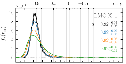
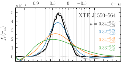
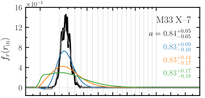
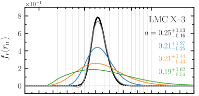
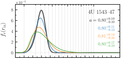
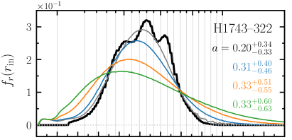
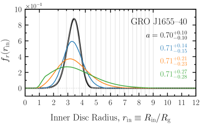
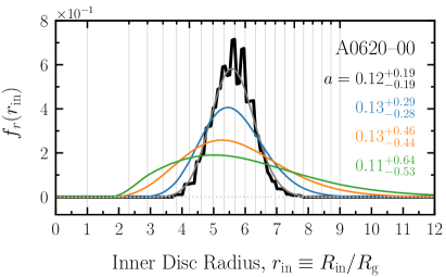
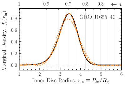
Figure 3: Inner disc radius marginal density fr​(rin)subscriptπ‘“π‘Ÿsubscriptπ‘Ÿinf_{r}(r_{\rm in}) for each X-ray binary in Table 1, which maps to a measurement of the black hole spin parameter aπ‘Ža (top xπ‘₯x-axis) assuming that rin=rISCOsubscriptπ‘Ÿinsubscriptπ‘ŸISCOr_{\rm in}=r_{\rm ISCO}. The thick black line shows the original disc continuum fitting measurement, which effectively adopts no uncertainty on the colour correction factor fcolsubscript𝑓colf_{\rm col} listed in Table 1. The line colour shows the revised black hole spin measurements after incorporating uncertainties in fcolsubscript𝑓colf_{\rm col} of Β±0.1plus-or-minus0.1\pm 0.1 (blue), Β±0.2plus-or-minus0.2\pm 0.2 (orange), and Β±0.3plus-or-minus0.3\pm 0.3 (green), assuming a normal distribution for its marginal density ff​(fcol)subscript𝑓𝑓subscript𝑓colf_{f}(f_{\rm col}) centered on the value in Table 1. The grey lines followed the same procedure as the coloured lines (see Β§3.1), but assumed no fcolsubscript𝑓colf_{\rm col} uncertainty, and they successfully recover the original measurements. Each legend gives the source name and quotes the spin measurement for each distribution, where the aπ‘Ža value corresponds to a cumulative density of 1/212\nicefrac{{1}}{{2}} (i.e., the median) and the uncertainty in aπ‘Ža corresponds to the inter-68% region of the marginal density. For most systems, including an fcolsubscript𝑓colf_{\rm col} uncertainty of Β±plus-or-minus\pm0.2–0.3 more than doubles the original quoted black hole spin uncertainties; thus, dominating the error budget if such fcolsubscript𝑓colf_{\rm col} uncertainty levels are reasonable (see Β§4.1).

For the eight X-ray binaries in Table 1 with a non-maximal black hole spin measurement from disc continuum fitting, the thick black line in Figure 3 shows the inner disc radius marginal density frCF​(rin)superscriptsubscriptπ‘“π‘ŸCFsubscriptπ‘Ÿinf_{r}^{\rm CF}(r_{\rm in}), which is synonymous with the black hole spin marginal density faCF​(a)superscriptsubscriptπ‘“π‘ŽCFπ‘Žf_{a}^{\rm CF}(a) under the usual rin=rISCOsubscriptπ‘Ÿinsubscriptπ‘ŸISCOr_{\rm in}=r_{\rm ISCO} assumption. We extracted published black hole spin measurements β€” that is, either faCF​(a)superscriptsubscriptπ‘“π‘ŽCFπ‘Žf_{a}^{\rm CF}(a) or frCF​(rin)superscriptsubscriptπ‘“π‘ŸCFsubscriptπ‘Ÿinf_{r}^{\rm CF}(r_{\rm in}) β€” using the DataThief program (Tummers, 2006) for the X-ray binaries: LMC X–1, XTE J1550–564, M33 X–7, LMC X–3, H1743–322, A0620–00. A black hole spin marginal density is not published for either 4U 1543–47 or GRO J1655–40, so in these cases we construct normal distributions for faCF​(a)superscriptsubscriptπ‘“π‘ŽCFπ‘Žf_{a}^{\rm CF}(a) based on the reported aCFsuperscriptπ‘ŽCFa^{\rm CF} values and uncertainties in Table 1.

Our aim is to incorporate uncertainties in the colour correction factor fcolsubscript𝑓colf_{\rm col} into each black hole spin measurement derived from disc continuum fitting. We accomplish this by combining probability density transformations with an inverse integral transform method and constrained optimization methods, with the details relegated to Appendix C and a summary provided below.

Starting with the black hole spin marginal density faCF​(a)superscriptsubscriptπ‘“π‘ŽCFπ‘Žf_{a}^{\rm CF}(a) reported from a disc continuum fitting measurement, we convert this to the inner disc radius marginal density frCF​(rin)superscriptsubscriptπ‘“π‘ŸCFsubscriptπ‘Ÿinf_{r}^{\rm CF}(r_{\rm in}) by assuming that rin=rISCOsubscriptπ‘Ÿinsubscriptπ‘ŸISCOr_{\rm in}=r_{\rm ISCO} and following Β§C.1. Next, we reverse-engineer frCF​(rin)superscriptsubscriptπ‘“π‘ŸCFsubscriptπ‘Ÿinf_{r}^{\rm CF}(r_{\rm in}) to obtain the marginal density of the disc flux normalization fK​(Kflux)subscript𝑓𝐾subscript𝐾fluxf_{K}(K_{\rm flux}), which is the observable quantity in our re-parametrized disc continuum fitting approach described in Β§2 and Appendix B. This requires inverting the integral transform equation

frCF​(rin)superscriptsubscriptπ‘“π‘ŸCFsubscriptπ‘Ÿin\displaystyle f_{r}^{\rm CF}\left(r_{\rm in}\right) =∫idisc=0Ο€/2∫D=0∞∫M=0βˆžπ‘‘M​𝑑D​𝑑idiscabsentsuperscriptsubscriptsubscript𝑖disc0πœ‹2superscriptsubscript𝐷0superscriptsubscript𝑀0differential-d𝑀differential-d𝐷differential-dsubscript𝑖disc\displaystyle=\int\limits_{i_{\rm disc}=0}^{\pi/2}\int\limits_{D=0}^{\infty}\int\limits_{M=0}^{\infty}dM~{}dD~{}di_{\rm disc}
Γ—fK​(hβˆ’1​(rin,fcolCF,M,D,idisc))absentsubscript𝑓𝐾superscriptβ„Ž1subscriptπ‘Ÿinsuperscriptsubscript𝑓colCF𝑀𝐷subscript𝑖disc\displaystyle\times f_{K}\left(h^{-1}\left(r_{\rm in},f_{\rm col}^{\rm CF},M,D,i_{\rm disc}\right)\right)
Γ—fM,D,i​(M,D,idisc)absentsubscript𝑓𝑀𝐷𝑖𝑀𝐷subscript𝑖disc\displaystyle\times f_{M,D,i}\left(M,D,i_{\rm disc}\right)
Γ—|J​(rin,fcolCF,M,D,idisc)|,absent𝐽subscriptπ‘Ÿinsuperscriptsubscript𝑓colCF𝑀𝐷subscript𝑖disc\displaystyle\times\left|J\left(r_{\rm in},f_{\rm col}^{\rm CF},M,D,i_{\rm disc}\right)\right|, (4)

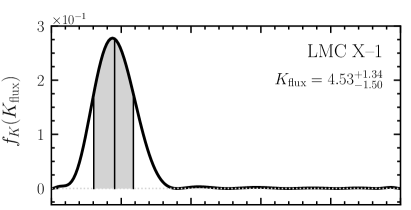
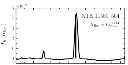
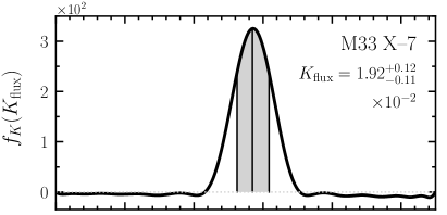
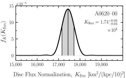
which follows from performing a multi-variate change of variables and then marginalizing over {fcol,M,D,idisc}subscript𝑓col𝑀𝐷subscript𝑖disc\{f_{\rm col},M,D,i_{\rm disc}\}. Importantly, we treat the marginal density ff​(fcol)subscript𝑓𝑓subscript𝑓colf_{f}(f_{\rm col}) as a Dirac delta function centered on the Table 1 value (denoted by fcolCFsuperscriptsubscript𝑓colCFf_{\rm col}^{\rm CF}) because that is effectively what the disc continuum fitting practitioners did when measuring frCF​(rin)superscriptsubscriptπ‘“π‘ŸCFsubscriptπ‘Ÿinf_{r}^{\rm CF}(r_{\rm in}). In equation (4), fM,D,i​(M,D,idisc)subscript𝑓𝑀𝐷𝑖𝑀𝐷subscript𝑖discf_{M,D,i}(M,D,i_{\rm disc}) is the joint density of the black hole mass, distance, and inner disc inclination; J​(rin,fcolCF,M,D,idisc)𝐽subscriptπ‘Ÿinsuperscriptsubscript𝑓colCF𝑀𝐷subscript𝑖discJ(r_{\rm in},f_{\rm col}^{\rm CF},M,D,i_{\rm disc}) is the Jacobian determinant for the change of variables from rinsubscriptπ‘Ÿinr_{\rm in} to Kfluxsubscript𝐾fluxK_{\rm flux}; and hβˆ’1​(rin,fcolCF,M,D,idisc)=Kfluxsuperscriptβ„Ž1subscriptπ‘Ÿinsuperscriptsubscript𝑓colCF𝑀𝐷subscript𝑖discsubscript𝐾fluxh^{-1}(r_{\rm in},f_{\rm col}^{\rm CF},M,D,i_{\rm disc})=K_{\rm flux} is the inverse transformation function, which is given by equation (2). Appendix C.2 derives equation (4) and goes on to explain the inversion methods (Β§C.2.1; Β§C.2.4) used to obtain fK​(Kflux)subscript𝑓𝐾subscript𝐾fluxf_{K}(K_{\rm flux}) in the integrand of equation (4).101010We note that the marginalization over {fcol,M,D,idisc}subscript𝑓col𝑀𝐷subscript𝑖disc\{f_{\rm col},M,D,i_{\rm disc}\} removes information. As such, the inversion of equation (4) is under-determined and fK​(Kflux)subscript𝑓𝐾subscript𝐾fluxf_{K}(K_{\rm flux}) is not unique. Figure 11 in the appendix shows the fK​(Kflux)subscript𝑓𝐾subscript𝐾fluxf_{K}(K_{\rm flux}) distributions calculated from this process for each X-ray binary system.

At this stage, we have successfully constructed fK​(Kflux)subscript𝑓𝐾subscript𝐾fluxf_{K}(K_{\rm flux}) in a way that is as consistent as possible with the reported disc continuum fitting black hole spin measurements. That is, our definition of Kfluxsubscript𝐾fluxK_{\rm flux} came from a re-parametrized disc model that is equivalent to the kerrbb model (see Β§2; Appendix B); we adopted the same joint density fM,D,i​(M,D,idisc)subscript𝑓𝑀𝐷𝑖𝑀𝐷subscript𝑖discf_{M,D,i}(M,D,i_{\rm disc}) used in making the reported spin measurements (see Β§2.1); and we did not incorporate any fcolsubscript𝑓colf_{\rm col} uncertainties (see Β§2.2). With fK​(Kflux)subscript𝑓𝐾subscript𝐾fluxf_{K}(K_{\rm flux}) in hand, we can now run the process described above in the opposite direction, but this time marginalizing over fcolsubscript𝑓colf_{\rm col} to produce an updated inner disc radius marginal density fr​(rin)subscriptπ‘“π‘Ÿsubscriptπ‘Ÿinf_{r}(r_{\rm in}) that includes fcolsubscript𝑓colf_{\rm col} uncertainties,

fr​(rin)subscriptπ‘“π‘Ÿsubscriptπ‘Ÿin\displaystyle f_{r}\left(r_{\rm in}\right) =∫fcol=1∞∫idisc=0Ο€/2∫D=0∞∫M=0βˆžπ‘‘M​𝑑D​𝑑idisc​𝑑fcolabsentsuperscriptsubscriptsubscript𝑓col1superscriptsubscriptsubscript𝑖disc0πœ‹2superscriptsubscript𝐷0superscriptsubscript𝑀0differential-d𝑀differential-d𝐷differential-dsubscript𝑖discdifferential-dsubscript𝑓col\displaystyle=\int\limits_{f_{\rm col}=1}^{\infty}\int\limits_{i_{\rm disc}=0}^{\pi/2}\int\limits_{D=0}^{\infty}\int\limits_{M=0}^{\infty}dM~{}dD~{}di_{\rm disc}~{}df_{\rm col}
Γ—fK​(hβˆ’1​(rin,fcol,M,D,idisc))absentsubscript𝑓𝐾superscriptβ„Ž1subscriptπ‘Ÿinsubscript𝑓col𝑀𝐷subscript𝑖disc\displaystyle\times f_{K}\left(h^{-1}\left(r_{\rm in},f_{\rm col},M,D,i_{\rm disc}\right)\right)
Γ—ff​(fcol)​fM,D,i​(M,D,idisc)absentsubscript𝑓𝑓subscript𝑓colsubscript𝑓𝑀𝐷𝑖𝑀𝐷subscript𝑖disc\displaystyle\times f_{f}\left(f_{\rm col}\right)f_{M,D,i}\left(M,D,i_{\rm disc}\right)
Γ—|J​(rin,fcol,M,D,idisc)|.absent𝐽subscriptπ‘Ÿinsubscript𝑓col𝑀𝐷subscript𝑖disc\displaystyle\times\left|J\left(r_{\rm in},f_{\rm col},M,D,i_{\rm disc}\right)\right|. (5)

Notably, equation (5) assumes that fcolsubscript𝑓colf_{\rm col} is independent of {M,D,idisc}𝑀𝐷subscript𝑖disc\{M,D,i_{\rm disc}\}, which may not be strictly true but is consistent with the relatively weak dependence of fcolsubscript𝑓colf_{\rm col} on these parameters in the bhspec model.111111See footnote 24 in Appendix C. Appendix C.3 describes how to obtain this β€œrevised” fr​(rin)subscriptπ‘“π‘Ÿsubscriptπ‘Ÿinf_{r}(r_{\rm in}) and its associated spin measurement fa​(a)subscriptπ‘“π‘Žπ‘Žf_{a}(a) from equation (5), which only differs from equation (4) by including uncertainties in fcolsubscript𝑓colf_{\rm col} through its marginal density ff​(fcol)subscript𝑓𝑓subscript𝑓colf_{f}(f_{\rm col}). The lower integration bound fcol=1subscript𝑓col1f_{\rm col}=1 arises because values of fcol<1subscript𝑓col1f_{\rm col}<1 are unphysical, so in practice we construct ff​(fcol)subscript𝑓𝑓subscript𝑓colf_{f}(f_{\rm col}) as a truncated distribution.

Evaluating the effects of fcolsubscript𝑓colf_{\rm col} uncertainties on a black hole spin measurement requires specifying the ff​(fcol)subscript𝑓𝑓subscript𝑓colf_{f}(f_{\rm col}) distribution. Investigations into the effects of various atmospheric physics (e.g., magnetic support, density inhomogeneities, vertical dissipation of accretion power) on the emergent disc spectrum warrant considering a systematic uncertainty on fcolsubscript𝑓colf_{\rm col} of Β±plus-or-minus\pm0.3 or perhaps even more (see Β§4.1). Lacking a good understanding of these uncertainties, we simply take fcolsubscript𝑓colf_{\rm col} to be normally distributed and centered on its value in Table 1 with a standard deviation of either 0.1, 0.2, or 0.3.121212We adopt symmetric uncertainties for simplicity’s sake and because different physical effects can conceivably drive fcolsubscript𝑓colf_{\rm col} in either direction (see Β§4.1). Asymmetric uncertainties may turn out to be more realistic, which are straightforward to incorporate.

Figure 3 is the culmination of this exercise, approximating the black hole spin measurements that would have been obtained had the disc continuum fitting practitioners incorporated an uncertainty on fcolsubscript𝑓colf_{\rm col} at the levels of Β±0.1plus-or-minus0.1\pm 0.1 (blue lines), Β±0.2plus-or-minus0.2\pm 0.2 (orange lines), or Β±0.3plus-or-minus0.3\pm 0.3 (green lines). As the uncertainty in fcolsubscript𝑓colf_{\rm col} increases, the peak of frsubscriptπ‘“π‘Ÿf_{r} shifts towards smaller rinsubscriptπ‘Ÿinr_{\rm in}, while the median of the distribution stays roughly the same. This has the effect of making frsubscriptπ‘“π‘Ÿf_{r} more asymmetric, with a sharper rise and longer tail.

In most cases, an fcolsubscript𝑓colf_{\rm col} uncertainty of Β±plus-or-minus\pm0.2–0.3 single-handedly dominates the black hole spin error budget,131313That is, the revised uncertainty range on the black hole spin is more than twice the original reported uncertainty range. which also includes uncertainties on {M,D,idisc}𝑀𝐷subscript𝑖disc\{M,D,i_{\rm disc}\} and Kfluxsubscript𝐾fluxK_{\rm flux}. Pairing the fcolsubscript𝑓colf_{\rm col} uncertainty level required to at least double the spin error budget with each individual source, we have: Β±0.1β†’β†’plus-or-minus0.1absent\pm 0.1\rightarrow None; Β±0.2β†’β†’plus-or-minus0.2absent\pm 0.2\rightarrow M33 X–7, GRO J1655–40, LMC X–3, A0620–00; Β±0.3β†’β†’plus-or-minus0.3absent\pm 0.3\rightarrow XTE J1550–564; while for an fcolsubscript𝑓colf_{\rm col} uncertainty of Β±0.3plus-or-minus0.3\pm 0.3, the spin error budget increases by 83% for H1743–322, 81% for 4U 1543–47, and 61% for LMC X–1. The grey lines, which correspond to incorporating zero uncertainty on fcolsubscript𝑓colf_{\rm col}, validate our methodology by successfully recovering the original black hole spin measurements β€” admittedly, XTE J1550–564 and H1743–322 are not perfect.

In Β§4, we make the case that a Β±0.2plus-or-minus0.2\pm 0.2–0.3 level of systematic uncertainty in fcolsubscript𝑓colf_{\rm col} is reasonable, given the current understanding of disc atmospheric physics.

3.2 Black Hole Spin Measurement Sensitivity to fcolsubscript𝑓colf_{\rm col}

The previous section supposed that the fcolsubscript𝑓colf_{\rm col} values listed in Table 1 are correct and demonstrated that uncertainties in an adopted fcolsubscript𝑓colf_{\rm col} value can significantly broaden the measured black hole spin marginal density. Here, we consider the possibility that an adopted fcolsubscript𝑓colf_{\rm col} value is incorrect due to systematic uncertainties associated with the bhspec model used to inform the choice for fcolsubscript𝑓colf_{\rm col}. We will use the same approach outlined in Β§3.1 to determine the sensitivity of the black hole spin measurements to different fcolsubscript𝑓colf_{\rm col} choices. Again, we stress that this approach cannot speak to whether an adopted fcolsubscript𝑓colf_{\rm col} value is in tension with the actual data; however, degeneracies among the kerrbb parameters can conceivably compensate for different fcolsubscript𝑓colf_{\rm col} choices to yield a statistically good fit to the data (e.g., Nowak etΒ al., 2008).

The grey lines in Figure 3 necessarily recover the original black hole spin measurements because they adopt the same fcolsubscript𝑓colf_{\rm col} values as in Table 1 and neglect fcolsubscript𝑓colf_{\rm col} uncertainty, as is effectively done by the disc continuum fitting practitioners. Maintaining this disregard for fcolsubscript𝑓colf_{\rm col} uncertainty throughout this section, the inner disc radius marginal density fr​(rin)subscriptπ‘“π‘Ÿsubscriptπ‘Ÿinf_{r}(r_{\rm in}) from equation (5) becomes

fr​(rin)subscriptπ‘“π‘Ÿsubscriptπ‘Ÿin\displaystyle f_{r}\left(r_{\rm in}\right) =∫idisc=0Ο€/2∫D=0∞∫M=0βˆžπ‘‘M​𝑑D​𝑑idiscabsentsuperscriptsubscriptsubscript𝑖disc0πœ‹2superscriptsubscript𝐷0superscriptsubscript𝑀0differential-d𝑀differential-d𝐷differential-dsubscript𝑖disc\displaystyle=\int\limits_{i_{\rm disc}=0}^{\pi/2}\int\limits_{D=0}^{\infty}\int\limits_{M=0}^{\infty}dM~{}dD~{}di_{\rm disc}
Γ—fK​(hβˆ’1​(rin,fcol,M,D,idisc))absentsubscript𝑓𝐾superscriptβ„Ž1subscriptπ‘Ÿinsubscript𝑓col𝑀𝐷subscript𝑖disc\displaystyle\times f_{K}\left(h^{-1}\left(r_{\rm in},f_{\rm col},M,D,i_{\rm disc}\right)\right)
Γ—fM,D,i​(M,D,idisc)absentsubscript𝑓𝑀𝐷𝑖𝑀𝐷subscript𝑖disc\displaystyle\times f_{M,D,i}\left(M,D,i_{\rm disc}\right)
Γ—|J​(rin,fcol,M,D,idisc)|,absent𝐽subscriptπ‘Ÿinsubscript𝑓col𝑀𝐷subscript𝑖disc\displaystyle\times\left|J\left(r_{\rm in},f_{\rm col},M,D,i_{\rm disc}\right)\right|, (6)

where we took ff​(fcol)subscript𝑓𝑓subscript𝑓colf_{f}(f_{\rm col}) to be a Dirac delta function centered on the new adopted value for fcolsubscript𝑓colf_{\rm col}.

Refer to caption
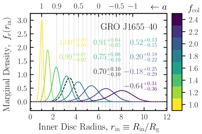
Figure 4: Inner disc radius marginal density fr​(rin)subscriptπ‘“π‘Ÿsubscriptπ‘Ÿinf_{r}(r_{\rm in}) for different choices of the colour correction factor fcolsubscript𝑓colf_{\rm col}, using GRO J1655–40 as an example. The top xπ‘₯x-axis shows the black hole spin parameter aπ‘Ža corresponding to rin=rISCOsubscriptπ‘Ÿinsubscriptπ‘ŸISCOr_{\rm in}=r_{\rm ISCO} and the dashed black line shows the original disc continuum fitting measurement. Increasing fcolsubscript𝑓colf_{\rm col} causes the measured black hole spin to decrease and broadens its marginal density. The colour-coded legend gives each black hole spin measurement, which changes substantially in response to modest changes in fcolsubscript𝑓colf_{\rm col}, especially for low-to-moderate spins.

Calculating fr​(rin)subscriptπ‘“π‘Ÿsubscriptπ‘Ÿinf_{r}(r_{\rm in}) from equation (6) with different choices of fcolsubscript𝑓colf_{\rm col} ranging from 1.0 to 2.4 in increments of 0.2, Figure 4 shows the corresponding black hole spin measurements that would be obtained for GRO J1655–40, as a representative example. Choosing a larger fcolsubscript𝑓colf_{\rm col} leads to a lower black hole spin measurement because the associated increase in rin∝fcol2proportional-tosubscriptπ‘Ÿinsuperscriptsubscript𝑓col2r_{\rm in}\propto f_{\rm col}^{2} (see equation 2) maps to a decrease in aπ‘Ža, under the assumption that rinsubscriptπ‘Ÿinr_{\rm in} coincides with the ISCO (see Figure 2). This strong degeneracy between fcolsubscript𝑓colf_{\rm col} and aπ‘Ža is well-known (e.g., Nowak etΒ al., 2008), but often goes under-appreciated, which compelled us to explicitly show how an erroneous choice for fcolsubscript𝑓colf_{\rm col} impacts the existing spin measurements.
Refer to caption
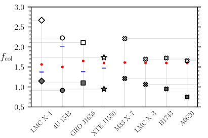
Figure 5: Colour correction factor fcolsubscript𝑓colf_{\rm col} for each X-ray binary in Table 1 that would yield a black hole spin measurement of a=0π‘Ž0a=0 (white symbols) and a=0.998π‘Ž0.998a=0.998 (dark symbols). Measuring a=0.998π‘Ž0.998a=0.998 is not possible in sources that require fcol<1subscript𝑓col1f_{\rm col}<1, which is unphysical. Vertical and horizontal lines help guide the eye. In most cases, 0.998>a>00.998π‘Ž00.998>a>0 is possible with 1.0<fcol≲2.21.0subscript𝑓colless-than-or-similar-to2.21.0<f_{\rm col}\lesssim 2.2. The red dots mark the fcolCFsuperscriptsubscript𝑓colCFf_{\rm col}^{\rm CF} values from Table 1 and the blue dashes mark the fcolsubscript𝑓colf_{\rm col} values needed to make aπ‘Ža consistent with the iron line spin measurements.

Although not shown, we repeat this exercise of varying fcolsubscript𝑓colf_{\rm col} and calculating fr​(rin)subscriptπ‘“π‘Ÿsubscriptπ‘Ÿinf_{r}(r_{\rm in}) for the eight X-ray binaries we consider. Figure 5 summarizes the results, showing the fcolsubscript𝑓colf_{\rm col} values that cause the measured black hole to be maximally-spinning (a=0.998π‘Ž0.998a=0.998; black symbols) and non-spinning (a=0π‘Ž0a=0; white symbols). The spin measurements for 4U 1543–47, XTE J1550–564, H1743–322, and A0620–00 cannot be made maximally-spinning by changing fcolsubscript𝑓colf_{\rm col} alone because this would require fcol<1subscript𝑓col1f_{\rm col}<1, which is unphysical. The moderate spin measurements in 4U 1543–47, GRO J1655-40, and M33 X–7 can be made non-spinning by adopting fcol≃2.2similar-to-or-equalssubscript𝑓col2.2f_{\rm col}\simeq 2.2. This result is seemingly inconsistent with fcol≳3greater-than-or-equivalent-tosubscript𝑓col3f_{\rm col}\gtrsim 3 (e.g., Begelman & Pringle, 2007), unless retrograde discs are common.

We also determined the fcolsubscript𝑓colf_{\rm col} values needed to bring the disc continuum fitting black hole spin measurements into agreement with those from the iron line method. These are: fcol=1.37subscript𝑓col1.37f_{\rm col}=1.37, 2.02, 1.38, 1.47 for LMC X–1, 4U 1543–47, GRO J1655–40, XTE J1550–564, respectively. Notably, the three systems with discrepant spin measurements cannot all be brought into agreement by applying a systematic shift in fcolsubscript𝑓colf_{\rm col}. Taken at face value, this suggests that different disc atmospheric physics might be operating in these systems to drive fcolsubscript𝑓colf_{\rm col} in different directions. Alternatively, other uncertainties inherent to the disc continuum fitting method (e.g., does idisc=iorbsubscript𝑖discsubscript𝑖orbi_{\rm disc}=i_{\rm orb}?), or the iron line method, or both as is often the case, could be responsible for the mismatched spins. Regardless, given the uncertainties in the continuum fitting method and the system parameters, Figure 5 is plausibly consistent with the relatively narrow range of fcol≃1.4similar-to-or-equalssubscript𝑓col1.4f_{\rm col}\simeq 1.4–1.8 predicted by spectral models (Davis etΒ al., 2005; Davis & El-Abd, 2019).

4 Discussion

Upon the inception of the disc continuum fitting concept for measuring black hole spin, Zhang etΒ al. (1997) recognized that, β€œThe largest theoretical uncertainty in [measuring the inner disc radius] is from fcolsubscript𝑓colf_{\rm col}.” Over two decades later, we think this still describes the situation today. The modern technique employs the gold standard in disc atmosphere models, which is commendable, but still uncertain, as discussed below.

4.1 Uncertainties in the Colour Correction Factor fcolsubscript𝑓colf_{\rm col}

Our discussion will focus on the degree to which disc atmospheric physics and its fcolsubscript𝑓colf_{\rm col} parametrization remains not fully understood, but first we point out that several other uncertainties abound with disc continuum fitting measurements of black hole spin. These include: reliance on an α𝛼\alpha-disc model, whereas other disc models might also provide good fits to the data; whether or not the inner disc truncates at the ISCO with a zero-torque boundary condition (e.g., Reynolds & Armitage, 2001); whether or not the inner disc inclination is interchangeable with the binary orbital or jet axes inclinations (e.g., Salvesen & Pokawanvit, 2020); contamination of the disc continuum Wien tail by a high-energy, non-thermal spectral component that is always present at some level (e.g., Kubota etΒ al., 2001); the role of bulk Comptonization of thermal disc photons by turbulent motions (e.g., Socrates etΒ al., 2004); and the role of heat transport mechanisms other than radiative diffusion, such as convection (e.g., Coleman etΒ al., 2017) or magnetic reconnection / flares (e.g., Beloborodov, 1999).

To its credit, the modern disc continuum fitting technique makes an educated fcolsubscript𝑓colf_{\rm col} choice for each spectral fit. This is done by tabulating fcolsubscript𝑓colf_{\rm col} on a grid of the two free parameters (MΛ™,a)Λ™π‘€π‘Ž(\dot{M},a) by fitting the colour-corrected kerrbb model to the physically-motivated bhspec model (see Β§2.2). The statistical uncertainty on fcolsubscript𝑓colf_{\rm col} from this fitting process can be roughly Β±0.03plus-or-minus0.03\pm 0.03, but is not considered, and choosing an effective viscosity Ξ±=0.01𝛼0.01\alpha=0.01 can systematically lower fcolsubscript𝑓colf_{\rm col} compared to Ξ±=0.1𝛼0.1\alpha=0.1 (see Figure 3 of Done & Davis, 2008). In most cases, practitioners perform two identical analyses with different fcolsubscript𝑓colf_{\rm col} grids, one tabulated with Ξ±=0.01𝛼0.01\alpha=0.01 and the other with Ξ±=0.1𝛼0.1\alpha=0.1, and then combine the two results into the reported black hole spin error budget. Figure 3 of Done & Davis (2008) shows that this practice amounts to including a systematic uncertainty on fcolsubscript𝑓colf_{\rm col}, but at a level of perhaps Β±0.02plus-or-minus0.02\pm 0.02 for m˙≲0.1less-than-or-similar-toΛ™π‘š0.1\dot{m}\lesssim 0.1, which is the relevant mΛ™Λ™π‘š\dot{m} for most cases, and as much as about Β±0.05plus-or-minus0.05\pm 0.05 for m˙≃0.3similar-to-or-equalsΛ™π‘š0.3\dot{m}\simeq 0.3. To be clear, our analysis assumed that no fcolsubscript𝑓colf_{\rm col} uncertainties went into the black hole spin error budget. But to be fair, fcolsubscript𝑓colf_{\rm col} uncertainties are probably included at about the Β±0.02plus-or-minus0.02\pm 0.02-level, but are not directly reported.

The salient point we want to make is that disc continuum fitting spin measurements effectively ignore fcolsubscript𝑓colf_{\rm col} uncertainties, by which we mean there are neglected systematics due to the model-dependence of bhspec that are potentially much larger than the nominal Β±0.02plus-or-minus0.02\pm 0.02-level. We now turn to the literature to demonstrate that fcolsubscript𝑓colf_{\rm col} uncertainties at the Β±plus-or-minus\pm0.2–0.3-level are reasonable, which we showed are generally enough to dominate the black hole spin error budget (see Figure 3).

Hints that there may be missing physics in the bhspec model come from the exquisite thermal component in LMC X–3, which cannot be reconciled with the predicted relativistically broadened absorption edges below ∼1​keVsimilar-toabsent1keV\sim 1~{}{\rm keV} (Kubota etΒ al., 2010).141414For observations lacking soft X-ray coverage, bhspec sometimes fits the data better than colour-corrected disc models like kerrbb (Davis etΒ al., 2006). The missing ingredient from bhspec might be a contribution from magnetic pressure support to the disc’s vertical hydrostatic balance, which reduces the strength of these edges as follows (see Blaes etΒ al., 2006): Increased magnetic pressure support alleviates the need for steep gas pressure gradients in combating the large magnitude of the vertical tidal gravitational acceleration at high disc altitudes. Consequently, magnetically supported discs have more vertically extended atmospheres with larger density scale heights and lower gas densities at the effective photosphere.151515See Appendix A for a discussion of the effective photosphere. Note that the ratio of the ionization rate to the recombination rate scales as N​ni/(ni​ne)𝑁subscript𝑛𝑖subscript𝑛𝑖subscript𝑛𝑒Nn_{i}/(n_{i}n_{e}), where N𝑁N is the number of ionizing photons and ni≃nesimilar-to-or-equalssubscript𝑛𝑖subscript𝑛𝑒n_{i}\simeq n_{e} are the ion and electron number densities. Therefore, a reduced gas density at the effective photosphere due to magnetic support corresponds to an increased ionization state of metals; thus, reducing the strength of absorption edges.

This same decrease in gas density at the effective photosphere Οβˆ—subscriptπœŒβˆ—\rho_{\ast}, combined with the increase in gas temperature Tβˆ—subscriptπ‘‡βˆ—T_{\ast}, associated with the inclusion of magnetic support also tends to harden the disc continuum, as follows. The blackbody spectrum produced at the effective photosphere emerges modified (see Appendix A), with the effective temperature hardened by an amount fcol∼(ΞΊesβˆ—/ΞΊthβˆ—)1/8similar-tosubscript𝑓colsuperscriptsuperscriptsubscriptπœ…esβˆ—superscriptsubscriptπœ…thβˆ—18f_{\rm col}\sim(\kappa_{\rm es}^{\ast}/\kappa_{\rm th}^{\ast})^{1/8}, where ΞΊesβˆ—/ΞΊthβˆ—βˆΟβˆ—βˆ’1​Tβˆ—7/2proportional-tosuperscriptsubscriptπœ…esβˆ—superscriptsubscriptπœ…thβˆ—superscriptsubscriptπœŒβˆ—1superscriptsubscriptπ‘‡βˆ—72\kappa_{\rm es}^{\ast}/\kappa_{\rm th}^{\ast}\propto\rho_{\ast}^{-1}T_{\ast}^{7/2} is the scaling of the scattering-to-absorption grey opacities, assuming Kramers’s opacity law. Applying the same radiative transfer code used in the bhspec model to the time- and horizontally-averaged vertical structure of a weakly magnetized radiation magnetohydrodynamic (MHD) shearing box simulation, Blaes etΒ al. (2006) found that including magnetic support indeed hardened the disc-integrated spectrum, with a best-fit fcol=1.74subscript𝑓col1.74f_{\rm col}=1.74, as compared to fcol=1.48subscript𝑓col1.48f_{\rm col}=1.48 without magnetic support.

On the other hand, magnetically supported disc surface layers are prone to Parker instabilities, which leads to large gas density inhomogeneities at the scattering and effective photospheres (Blaes etΒ al., 2007). Interestingly, in the weakly magnetized regime accessible to zero-net vertical flux MHD simulations, the characteristic ∼10%similar-toabsentpercent10\sim 10\% increase in fcolsubscript𝑓colf_{\rm col} from magnetic pressure support is compensated by a ∼10%similar-toabsentpercent10\sim 10\% decrease from density inhomogeneities (Davis etΒ al., 2009). This softening results from the denser regions enhancing the overall emissivity (because ϡνff∝ρ2proportional-tosuperscriptsubscriptitalic-ϡ𝜈ffsuperscript𝜌2\epsilon_{\nu}^{\rm ff}\propto\rho^{2}), as follows. The total liberated gravitational energy gets partitioned into more photons that individually carry less energy, as compared to a homogeneous medium with a lower emissivity and hence fewer photons to carry the same total energy. Consequently, in an inhomogeneous medium the radiation temperature is lower, which means the spectrum is softer. A typical photon produced at the effective photosphere is then able to scatter to a low density region (because ΞΊes≫κthmuch-greater-thansubscriptπœ…essubscriptπœ…th\kappa_{\rm es}\gg\kappa_{\rm th}) from which it is more likely to escape before being absorbed.

The aforementioned studies of how magnetic fields affect the emergent disc spectrum used disc structures from shearing box simulations with weak magnetization; that is, the ratio of gas-to-magnetic pressures β≑Pgas/Pmagβ‰ͺ1𝛽subscript𝑃gassubscript𝑃magmuch-less-than1\beta\equiv P_{\rm gas}/P_{\rm mag}\ll 1 at the disc mid-plane. It remains to be seen whether or not the hardening/softening balance between magnetic support and density inhomogeneities extends to more strongly magnetized regimes, which dramatically influence the disc structure (e.g., Salvesen etΒ al., 2016; Mishra etΒ al., 2020).

Crude estimates suggest that fcolsubscript𝑓colf_{\rm col} might achieve extreme values for strong disc magnetizations. Extending the α𝛼\alpha-disc model to the magnetic pressure-dominated regime (Pariev etΒ al., 2003), then assuming LTE inside the disc and that radiative diffusion transports the liberated gravitational energy outward, Begelman & Pringle (2007) found the scaling of the lower limit on the colour correction factor to be

fcol≳3.4​(Ξ±1)5/27​(m10)βˆ’1/108​(mΛ™0.1)5/108​(x20)βˆ’25/108greater-than-or-equivalent-tosubscript𝑓col3.4superscript𝛼1527superscriptπ‘š101108superscriptΛ™π‘š0.15108superscriptπ‘₯2025108f_{\rm col}\gtrsim 3.4~{}\left(\frac{\alpha}{1}\right)^{5/27}\left(\frac{m}{10}\right)^{-1/108}\left(\frac{\dot{m}}{0.1}\right)^{5/108}\left(\frac{x}{20}\right)^{-25/108}

in the maximum field strength limit (Pessah & Psaltis, 2005), which suggests that strongly magnetized discs have very large colour temperatures. Here, m≑M/MβŠ™π‘šπ‘€subscript𝑀direct-productm\equiv M/M_{\odot}, m˙≑MΛ™/MΛ™EddΛ™π‘šΛ™π‘€subscript˙𝑀Edd\dot{m}\equiv\dot{M}/\dot{M}_{\rm Edd}, and x≑R/Rgπ‘₯𝑅subscript𝑅gx\equiv R/R_{\rm g}. Importantly, we include the radiative efficiency factor (adopting Ξ·=0.057πœ‚0.057\eta=0.057) in the Eddington mass accretion rate MΛ™Edd=LEdd/(η​c2)subscript˙𝑀Eddsubscript𝐿Eddπœ‚superscript𝑐2\dot{M}_{\rm Edd}=L_{\rm Edd}/(\eta c^{2}), where LEdd=4​π​G​M​mp​c/ΟƒTsubscript𝐿Edd4πœ‹πΊπ‘€subscriptπ‘šp𝑐subscript𝜎TL_{\rm Edd}=4\pi GMm_{\rm p}c/\sigma_{\rm T} is the Eddington luminosity. This way, mΛ™Λ™π‘š\dot{m} is equivalent to l≑Ldisc/LEdd𝑙subscript𝐿discsubscript𝐿Eddl\equiv L_{\rm disc}/L_{\rm Edd}, where Ldisc=η​M˙​c2subscript𝐿discπœ‚Λ™π‘€superscript𝑐2L_{\rm disc}=\eta\dot{M}c^{2} is the disc luminosity.161616Disc structure models sometimes omit Ξ·πœ‚\eta in their definition of mΛ™Λ™π‘š\dot{m} (e.g., Svensson & Zdziarski, 1994; Begelman & Pringle, 2007). We chose Ξ±=1𝛼1\alpha=1 as representative based on results from magnetic pressure-dominated shearing box simulations (Salvesen etΒ al., 2016). For comparison, we find that the same analysis for a non-magnetized, radiation pressure-dominated disc structure gives the much lower lower limit (Shakura & Sunyaev, 1973; Svensson & Zdziarski, 1994)

fcol≳1.7​(Ξ±0.1)2/9​(m10)1/36​(mΛ™0.1)23/36​(x20)βˆ’11/12.greater-than-or-equivalent-tosubscript𝑓col1.7superscript𝛼0.129superscriptπ‘š10136superscriptΛ™π‘š0.12336superscriptπ‘₯201112f_{\rm col}\gtrsim 1.7~{}\left(\frac{\alpha}{0.1}\right)^{2/9}\left(\frac{m}{10}\right)^{1/36}\left(\frac{\dot{m}}{0.1}\right)^{23/36}\left(\frac{x}{20}\right)^{-11/12}.

By neglecting the effect of thermal Comptonization to down-scatter escaping photons into a Wien-like spectrum, Begelman & Pringle (2007) overestimate fcolsubscript𝑓colf_{\rm col} for the magnetically dominated regime they consider. One expects Comptonization to be important for large fcolsubscript𝑓colf_{\rm col} because the number of scatterings experienced by a photon escaping from the effective photosphere is approximately NβˆΌΟ„βˆ—2∼fcol8similar-to𝑁superscriptsubscriptπœβˆ—2similar-tosuperscriptsubscript𝑓col8N\sim\tau_{\ast}^{2}\sim f_{\rm col}^{8}. This strong fcolsubscript𝑓colf_{\rm col} scaling comes from fcol∼Tβˆ—/TeffβˆΌΟ„βˆ—1/4similar-tosubscript𝑓colsubscriptπ‘‡βˆ—subscript𝑇effsimilar-tosuperscriptsubscriptπœβˆ—14f_{\rm col}\sim T_{\ast}/T_{\rm eff}\sim\tau_{\ast}^{1/4} (see Appendix A). Following a similar analysis to Begelman & Pringle (2007) in estimating fcolsubscript𝑓colf_{\rm col}, we estimate the Compton y𝑦y-parameter yβˆ—β‰‘4​kB​Tβˆ—/(me​c2)​max⁑(Ο„βˆ—2,Ο„βˆ—)subscriptπ‘¦βˆ—4subscriptπ‘˜Bsubscriptπ‘‡βˆ—subscriptπ‘šesuperscript𝑐2superscriptsubscriptπœβˆ—2subscriptπœβˆ—y_{\ast}\equiv 4k_{\rm B}T_{\ast}/(m_{\rm e}c^{2})\max(\tau_{\ast}^{2},\tau_{\ast}) at the optically thick (Ο„βˆ—β‰«1much-greater-thansubscriptπœβˆ—1\tau_{\ast}\gg 1) effective photosphere to be

yβˆ—=4​kB​Tme​c2​τesβˆ’2​(ΞΊbfΞΊes)βˆ’2​(Οβˆ—Ο)βˆ’2,subscriptπ‘¦βˆ—4subscriptπ‘˜B𝑇subscriptπ‘šesuperscript𝑐2superscriptsubscript𝜏es2superscriptsubscriptπœ…bfsubscriptπœ…es2superscriptsubscriptπœŒβˆ—πœŒ2y_{\ast}=\frac{4k_{\rm B}T}{m_{\rm e}c^{2}}\tau_{\rm es}^{-2}\left(\frac{\kappa_{\rm bf}}{\kappa_{\rm es}}\right)^{-2}\left(\frac{\rho_{\ast}}{\rho}\right)^{-2},

where T𝑇T, ρ𝜌\rho, and Ο„essubscript𝜏es\tau_{\rm es} are the gas temperature, gas density, and electron scattering optical depth, all at the disc mid-plane. Evaluating the Kramers’s bound-free opacity for solar abundances, ΞΊbf=1.6Γ—1024​ρ​Tβˆ’7/2​cm2​gβˆ’1subscriptπœ…bf1.6superscript1024𝜌superscript𝑇72superscriptcm2superscriptg1\kappa_{\rm bf}=1.6\times 10^{24}\rho T^{-7/2}~{}{\rm cm^{2}~{}g^{-1}}, at the disc mid-plane and adopting an electron scattering opacity ΞΊes=0.4​cm2​gβˆ’1subscriptπœ…es0.4superscriptcm2superscriptg1\kappa_{\rm es}=0.4~{}{\rm cm^{2}~{}g^{-1}}, we find that in the maximally magnetized limit (Begelman & Pringle, 2007),

yβˆ—β‰³1.4Γ—102​(Ξ±1)5/3​(m10)βˆ’1/3​(mΛ™0.1)2/3​(x20)βˆ’17/6,greater-than-or-equivalent-tosubscriptπ‘¦βˆ—1.4superscript102superscript𝛼153superscriptπ‘š1013superscriptΛ™π‘š0.123superscriptπ‘₯20176y_{\ast}\gtrsim 1.4\times 10^{2}~{}\left(\frac{\alpha}{1}\right)^{5/3}\left(\frac{m}{10}\right)^{-1/3}\left(\frac{\dot{m}}{0.1}\right)^{2/3}\left(\frac{x}{20}\right)^{-17/6},

with the lower limit being because Οβˆ—/ρ<1subscriptπœŒβˆ—πœŒ1\rho_{\ast}/\rho<1. Figures 1b, 2b, and 3b in Shimura & Takahara (1995) compare the yβˆ—β‰«1much-greater-thansubscriptπ‘¦βˆ—1y_{\ast}\gg 1 inner disc annuli to the yβˆ—β‰ͺ1much-less-thansubscriptπ‘¦βˆ—1y_{\ast}\ll 1 outer disc annuli, finding only a mild fcolsubscript𝑓colf_{\rm col} reduction attributed to thermal Comptonization. The extent to which Comptonization limits large fcolsubscript𝑓colf_{\rm col} in the magnetically dominated regime may be more severe, but understanding the degree to which thermal Comptonization reduces fcolsubscript𝑓colf_{\rm col} requires knowledge of the detailed vertical disc structure (e.g., the gas temperature at the location where y=1𝑦1y=1).

The low gas density Οβˆ—subscriptπœŒβˆ—\rho_{\ast} at the effective photosphere is a principle driver of the large fcolsubscript𝑓colf_{\rm col} estimates from magnetically dominated discs. A related quantity is the mid-plane column mass m0subscriptπ‘š0m_{0}, with the Begelman & Pringle (2007) model predicting

m0∼1.2Γ—102​(Ξ±1)βˆ’8/9​(m10)1/9​(mΛ™0.1)7/9​(x20)βˆ’5/9​g​cmβˆ’2.similar-tosubscriptπ‘š01.2superscript102superscript𝛼189superscriptπ‘š1019superscriptΛ™π‘š0.179superscriptπ‘₯2059gsuperscriptcm2m_{0}\sim 1.2\times 10^{2}~{}\left(\frac{\alpha}{1}\right)^{-8/9}\left(\frac{m}{10}\right)^{1/9}\left(\frac{\dot{m}}{0.1}\right)^{7/9}\left(\frac{x}{20}\right)^{-5/9}~{}{\rm g~{}cm^{-2}}.

Like yβˆ—subscriptπ‘¦βˆ—y_{\ast}, the expected m0subscriptπ‘š0m_{0} is sensitive to α𝛼\alpha. Although the existing disc atmosphere models lack magnetic pressure support, they do span a large range of m0subscriptπ‘š0m_{0} down to 102.5​g​cmβˆ’2superscript102.5gsuperscriptcm210^{2.5}~{}{\rm g~{}cm^{-2}} and find that fcol≲2.0less-than-or-similar-tosubscript𝑓col2.0f_{\rm col}\lesssim 2.0 for mΛ™βˆΌ0.1similar-toΛ™π‘š0.1\dot{m}\sim 0.1 (e.g., Davis & El-Abd, 2019). Based on this m0subscriptπ‘š0m_{0} parameter study, the very large fcolsubscript𝑓colf_{\rm col} values predicted for magnetically dominated discs might not be plausible.

Besides magnetization, several other pieces of β€œmissing physics” from bhspec can affect fcolsubscript𝑓colf_{\rm col}, with different degrees of importance. Encouragingly for disc continuum fitting applications, when most of the accretion power gets dissipated below the effective photosphere, the vertical dissipation profile has little impact on fcolsubscript𝑓colf_{\rm col} (Davis etΒ al., 2005; Blaes etΒ al., 2006). If instead some fraction Ο‡πœ’\chi of the accretion energy is dissipated in a corona, then the disc becomes colder, denser, and optically thicker (Svensson & Zdziarski, 1994). These effects conspire to produce a softer disc spectrum, where an example calculation showed that depositing 80% of the accretion energy into the corona, but neglecting its irradiation on the disc, decreased fcolsubscript𝑓colf_{\rm col} from 1.62 to 1.43 (Davis & El-Abd, 2019).171717Davis & El-Abd (2019) offer plausible explanations for why Merloni etΒ al. (2000) reported the opposite trend of increasing fcolsubscript𝑓colf_{\rm col} with increasing Ο‡πœ’\chi. Less explored are the effects on the disc continuum from non-solar metallicity, bound-bound opacities, and irradiation from a corona and/or returning radiation (e.g., Cunningham, 1976). Finally, current models cannot simultaneously consider the three-dimensional (3D) local disc structure and treat the radiative transfer self-consistently: bhspec is self-consistent, at the expense of only considering the vertical disc structure (Davis & Hubeny, 2006); while Monto Carlo radiative transfer post-processing of 3D shearing box data sacrifices self-consistency (Davis etΒ al., 2009).

4.2 Path Forward: The Case for Disc Magnetization

The discussion above harps on the need to better understand how various physics affect fcolsubscript𝑓colf_{\rm col}. Perhaps more difficult is deciding what physics is most relevant to real black hole X-ray binary systems in the high/soft state, where disc continuum fitting is appropriate. Here, we offer several pieces of evidence that warrant future studies on how magnetic fields influence the disc spectrum.

Disc accretion in X-ray binaries is a fundamentally magnetic process; that is, the magneto-rotational instability (MRI) generates turbulence in the disc and mediates angular momentum transport that drives accretion (Balbus & Hawley, 1991). The MRI establishes the critical role of magnetic fields in X-ray binaries and its saturation sets toroidal field strength extrema (e.g., Hawley etΒ al., 1995; Das etΒ al., 2018). Beyond that, magnetization remains perhaps the least understood aspect of disc physics, with the field strength, topology, and dynamical importance being open areas of active study.

A compelling case for dynamically important magnetic fields is made by the highly-ionized, blue-shifted absorption lines from the GRO J1655-40 disc wind, which cannot be explained without invoking a magnetic-driving mechanism (Miller etΒ al., 2006; Balakrishnan etΒ al., 2020). Strong magnetic fields (B∼103similar-to𝐡superscript103B\sim 10^{3}–105superscript10510^{5} G) are also required to drive the GRS 1915+105 disc wind in the high/soft state when the mass accretion rate mΛ™Λ™π‘š\dot{m} is large (Miller etΒ al., 2016), but a β€œfailed” disc wind is observed at lower mΛ™Λ™π‘š\dot{m} (Miller etΒ al., 2020). Speculatively, this variable disc wind may be consistent with the idea that mΛ™Λ™π‘š\dot{m} regulates the field strength (e.g., Begelman & Armitage, 2014), such that a decrease in mΛ™Λ™π‘š\dot{m} diminishes inward advection and the resulting weaker field cannot accelerate a wind to escape from the inner disc regions.

Light curve modeling of black hole X-ray binary outbursts favor a large effective viscosity α≃0.2similar-to-or-equals𝛼0.2\alpha\simeq 0.2 (Tetarenko etΒ al., 2018), which large-scale poloidal magnetic fields threading the disc naturally provides (e.g., Hawley etΒ al., 1995; Salvesen etΒ al., 2016). Another attractive property of magnetic pressure-dominated discs is that they are not prone to thermal or viscous instabilities (e.g., Begelman & Pringle, 2007; Jiang etΒ al., 2019), unlike radiation pressure-dominated discs (Shakura & Sunyaev, 1976; Lightman & Eardley, 1974), which is consistent with the steady disc emission (as opposed to limit cycle behaviour) observed in the high/soft state.


The goal of this discussion was to show that an fcolsubscript𝑓colf_{\rm col} uncertainty of Β±plus-or-minus\pm0.2–0.3 is a plausible level to include in the black hole spin error budget. For the disc accretion regimes relevant to X-ray binaries in the high/soft state, the current best theoretical understanding is that fcolsubscript𝑓colf_{\rm col} can span ≃1.4similar-to-or-equalsabsent1.4\simeq 1.4–2.0 (e.g., Davis etΒ al., 2005; Davis & El-Abd, 2019). Observational attempts to measure fcolsubscript𝑓colf_{\rm col} are consistent with this range, but very uncertain (see Β§1). The case for larger fcolsubscript𝑓colf_{\rm col} is much more speculative.

Theoretically, fcol>2.0subscript𝑓col2.0f_{\rm col}>2.0 either requires strong magnetization (Begelman & Pringle, 2007); or α∼1similar-to𝛼1\alpha\sim 1 (Davis & El-Abd, 2019), as seen in magnetic pressure-dominated shearing box simulations (Salvesen etΒ al., 2016); or the disc surface density to be low enough to make it β€œphoton starved,” meaning that the resulting lowered emissivity cannot radiate away the liberated gravitational energy and the radiation temperature must increase to compensate (Davis & El-Abd, 2019). Observationally, a static fcolsubscript𝑓colf_{\rm col} is not consistent with an inner disc edge truncated out to ≳100​Rggreater-than-or-equivalent-toabsent100subscript𝑅g\gtrsim 100~{}R_{\rm g} that migrates inwards as the source softens (Reynolds & Miller, 2013). Instead, the alternative interpretation that the inner disc edge remains near the ISCO during state transitions implies a dynamic fcolsubscript𝑓colf_{\rm col} that varies by a factor of ∼similar-to\sim2.0–3.5 (Salvesen etΒ al., 2013).

Regardless of whether fcolsubscript𝑓colf_{\rm col} can reach such extremes, the discussion above justifies our representative fcolsubscript𝑓colf_{\rm col} uncertainties of Β±plus-or-minus\pm0.2–0.3, which are enough to dominate the uncertainty in black hole spin measurements made with the disc continuum fitting technique (see Figure 3).

5 Summary and Conclusions

The disc continuum fitting community reports black hole spin measurements that meet certain quality criteria for 10 different X-ray binaries (McClintock etΒ al., 2014), but the reported spins effectively do not marginalize over the colour correction factor fcolsubscript𝑓colf_{\rm col} (see Β§2.2). By re-parametrizing the disc continuum model in terms of a disc flux normalization Kfluxsubscript𝐾fluxK_{\rm flux} (see Β§2; Appendix B), we reverse-engineered each of the eight non-maximal black hole spin marginal densities to obtain the marginal density fK​(Kflux)subscript𝑓𝐾subscript𝐾fluxf_{K}(K_{\rm flux}) (see Β§3; Appendix C), which we treat as the observable. Combining uncertainties on all parameters in the disc continuum model, including fcolsubscript𝑓colf_{\rm col}, we presented revised black hole spin measurements with different choices for either the fcolsubscript𝑓colf_{\rm col} uncertainty level (see Β§3.1) or the adopted fcolsubscript𝑓colf_{\rm col} value (see Β§3.2). From this analysis, our conclusions are that:

  • β€’

    Adopting systematic uncertainties on fcolsubscript𝑓colf_{\rm col} at the level of Β±0.2plus-or-minus0.2\pm 0.2–0.3 is reasonable (see Β§4) and enough to dominate the error budget of most black hole spin measurements from disc continuum fitting (see Figure 3).

  • β€’

    The measured black hole spin decreases precipitously with increasing fcolsubscript𝑓colf_{\rm col} (see Figure 4). A systematic offset between the adopted fcolsubscript𝑓colf_{\rm col} and its β€œactual value” will lead to an erroneous black hole spin measurement, especially for low-to-moderate intrinsic spins.

  • β€’

    Of the six X-ray binaries with vetted black hole spin measurements from two independent techniques, the three non-extremal cases (i.e., a<0.9π‘Ž0.9a<0.9) are discrepant at the 68%percent6868\%-level (see Figure 1). Incorporating fcolsubscript𝑓colf_{\rm col} uncertainties may help alleviate this tension, as the discrepant sources could be brought into agreement with fcolsubscript𝑓colf_{\rm col} values in the range 1.4≀fcol≀2.01.4subscript𝑓col2.01.4\leq f_{\rm col}\leq 2.0.

The widespread success of disc continuum fitting applications to X-ray binaries in the high/soft state is a testament to the applicability of a colour-corrected, multi-temperature, disc blackbody model in this accretion regime. However, using this disc model to measure physical parameters of the system, like the black hole spin, requires a firm understanding of its phenomenological parametrization in terms of fcolsubscript𝑓colf_{\rm col}. Reporting accurate measurements requires knowledge and inclusion of the fcolsubscript𝑓colf_{\rm col} uncertainties, both statistical and systematic. Statistical uncertainties refer to the validity of a colour-corrected approximation to the true disc continuum (e.g., kerrbb fits to bhspec models are not perfect). Systematic uncertainties refer to the possibility that the physical disc atmosphere model (e.g., bhspec) being used to inform the choices for fcolsubscript𝑓colf_{\rm col} is missing potentially relevant physics, such as the effects of magnetization. To better understand how disc atmospheric physics affects the observed spectrum, the path forward might involve local and global numerical simulations of thin discs that self-consistently treat magnetohydrodynamics and frequency-dependent radiative transfer, which may soon be possible with state-of-the art codes like MOCMC (Ryan & Dolence, 2020).

Acknowledgements

We are grateful to the anonymous referee for their constructive feedback. GS appreciates the helpful comments and suggestions from an anonymous referee on a withdrawn draft. We thank Mitch Begelman, Omer Blaes, Eric Coughlin, Josh Dolence, Brooks Kinch, Tom Maccarone, Jon Miller, Jordan Mirocha, and Ben Ryan for productive discussions, along with Robert Feldmann for helpful e-mail exchanges. GS acknowledges support through an NSF Astronomy & Astrophysics Postdoctoral Fellowship under award AST-1602169 and the NASA Earth and Space Science Graduate Fellowship program.

This work was supported by the US Department of Energy through the Los Alamos National Laboratory (LANL). Additional funding was provided by the Laboratory Directed Research and Development Program and the Center for Space and Earth Science (CSES) at LANL under project numbers 20190021DR and 20180475DR (TS). This research used resources provided by the LANL Institutional Computing Program. LANL is operated by Triad National Security, LLC, for the National Nuclear Security Administration of U.S. Department of Energy under Contract No. 89233218CNA000001. LANL assigned this article the document release number LA-UR-20-28487.

Software: We are grateful to the countless developers contributing to open source projects on which this work relied, including Python (Rossum, 1995), NumPy and SciPy (Oliphant, 2006; Virtanen etΒ al., 2020), Matplotlib (Hunter, 2007), HDF5 (The HDF Group, 1997-2019), and DataThief (Tummers, 2006).

Data Availability: The data and code used in this paper are available as a GitHub repository: https://github.com/gregsalvesen/bhspinf. If this link goes defunct, contact the corresponding author to request access to the data and code. LANL approved the data and code for open source distribution under data release number LA-UR-20-28697 and the BSD-3 License, respectively.

References

  • Arnaud (1996) Arnaud, K.Β A. 1996, in Astronomical Society of the Pacific Conference Series, Vol. 101, Astronomical Data Analysis Software and Systems V, ed. G.Β H.Β Jacoby & J.Β Barnes, 17
  • Balakrishnan etΒ al. (2020) Balakrishnan, M., Miller, J.Β M., Trueba, N., etΒ al. 2020, ApJ, 893, 155, doi:Β 10.3847/1538-4357/ab8304
  • Balbus & Hawley (1991) Balbus, S.Β A., & Hawley, J.Β F. 1991, ApJ, 376, 214, doi:Β 10.1086/170270
  • Bardeen etΒ al. (1972) Bardeen, J.Β M., Press, W.Β H., & Teukolsky, S.Β A. 1972, ApJ, 178, 347, doi:Β 10.1086/151796
  • Begelman & Armitage (2014) Begelman, M.Β C., & Armitage, P.Β J. 2014, ApJ, 782, L18, doi:Β 10.1088/2041-8205/782/2/L18
  • Begelman & Pringle (2007) Begelman, M.Β C., & Pringle, J.Β E. 2007, MNRAS, 375, 1070, doi:Β 10.1111/j.1365-2966.2006.11372.x
  • Belloni (2010) Belloni, T.Β M. 2010, in Lecture Notes in Physics, Berlin Springer Verlag, Vol. 794, Lecture Notes in Physics, Berlin Springer Verlag, ed. T.Β Belloni, 53, doi:Β 10.1007/978-3-540-76937-8_3
  • Beloborodov (1999) Beloborodov, A.Β M. 1999, ApJ, 510, L123, doi:Β 10.1086/311810
  • Blaes etΒ al. (2007) Blaes, O., Hirose, S., & Krolik, J.Β H. 2007, ApJ, 664, 1057, doi:Β 10.1086/519516
  • Blaes etΒ al. (2006) Blaes, O.Β M., Davis, S.Β W., Hirose, S., Krolik, J.Β H., & Stone, J.Β M. 2006, ApJ, 645, 1402, doi:Β 10.1086/503741
  • Blandford & Znajek (1977) Blandford, R.Β D., & Znajek, R.Β L. 1977, MNRAS, 179, 433
  • Blum etΒ al. (2009) Blum, J.Β L., Miller, J.Β M., Fabian, A.Β C., etΒ al. 2009, ApJ, 706, 60, doi:Β 10.1088/0004-637X/706/1/60
  • Boyd (2013) Boyd, J. 2013, Chebyshev and Fourier Spectral Methods: Second Revised Edition, Dover Books on Mathematics (Dover Publications). https://books.google.com/books?id=b4TCAgAAQBAJ
  • Byrd etΒ al. (1995) Byrd, R.Β H., Lu, P., Nocedal, J., & Zhu, C. 1995, SIAM Journal on scientific computing, 16, 1190
  • Cantrell etΒ al. (2010) Cantrell, A.Β G., Bailyn, C.Β D., Orosz, J.Β A., etΒ al. 2010, ApJ, 710, 1127, doi:Β 10.1088/0004-637X/710/2/1127
  • Chandrasekhar (1960) Chandrasekhar, S. 1960, Radiative transfer
  • Coleman etΒ al. (2017) Coleman, M. S.Β B., Yerger, E., Blaes, O., Salvesen, G., & Hirose, S. 2017, MNRAS, 467, 2625, doi:Β 10.1093/mnras/stx268
  • Cunningham (1976) Cunningham, C. 1976, ApJ, 208, 534, doi:Β 10.1086/154636
  • Cunningham (1975) Cunningham, C.Β T. 1975, ApJ, 202, 788, doi:Β 10.1086/154033
  • Das etΒ al. (2018) Das, U., Begelman, M.Β C., & Lesur, G. 2018, MNRAS, 473, 2791, doi:Β 10.1093/mnras/stx2518
  • Davis etΒ al. (2009) Davis, S.Β W., Blaes, O.Β M., Hirose, S., & Krolik, J.Β H. 2009, ApJ, 703, 569, doi:Β 10.1088/0004-637X/703/1/569
  • Davis etΒ al. (2005) Davis, S.Β W., Blaes, O.Β M., Hubeny, I., & Turner, N.Β J. 2005, ApJ, 621, 372, doi:Β 10.1086/427278
  • Davis etΒ al. (2006) Davis, S.Β W., Done, C., & Blaes, O.Β M. 2006, ApJ, 647, 525, doi:Β 10.1086/505386
  • Davis & El-Abd (2019) Davis, S.Β W., & El-Abd, S. 2019, ApJ, 874, 23, doi:Β 10.3847/1538-4357/ab05c5
  • Davis & Hubeny (2006) Davis, S.Β W., & Hubeny, I. 2006, ApJS, 164, 530, doi:Β 10.1086/503549
  • Davison & Sykes (1957) Davison, B., & Sykes, J. 1957, Neutron Transport Theory, International series of monographs on physics (Clarendon Press). https://books.google.com/books?id=ZhlRAAAAMAAJ
  • Done & Davis (2008) Done, C., & Davis, S.Β W. 2008, ApJ, 683, 389, doi:Β 10.1086/589647
  • Dong etΒ al. (2020) Dong, Y., GarcΓ­a, J.Β A., Steiner, J.Β F., & Gou, L. 2020, MNRAS, 493, 4409, doi:Β 10.1093/mnras/staa606
  • Esin etΒ al. (1997) Esin, A.Β A., McClintock, J.Β E., & Narayan, R. 1997, ApJ, 489, 865, doi:Β 10.1086/304829
  • Fabian etΒ al. (1989) Fabian, A.Β C., Rees, M.Β J., Stella, L., & White, N.Β E. 1989, MNRAS, 238, 729
  • Fabian etΒ al. (2012) Fabian, A.Β C., Wilkins, D.Β R., Miller, J.Β M., etΒ al. 2012, MNRAS, 424, 217, doi:Β 10.1111/j.1365-2966.2012.21185.x
  • Felten & Rees (1972) Felten, J.Β E., & Rees, M.Β J. 1972, A&A, 17, 226
  • Fender etΒ al. (1999) Fender, R.Β P., Garrington, S.Β T., McKay, D.Β J., etΒ al. 1999, MNRAS, 304, 865, doi:Β 10.1046/j.1365-8711.1999.02364.x
  • Fragile etΒ al. (2007) Fragile, P.Β C., Blaes, O.Β M., Anninos, P., & Salmonson, J.Β D. 2007, ApJ, 668, 417, doi:Β 10.1086/521092
  • Frank etΒ al. (2002) Frank, J., King, A., & Raine, D.Β J. 2002, Accretion Power in Astrophysics: Third Edition
  • Fukue & Akizuki (2006) Fukue, J., & Akizuki, C. 2006, PASJ, 58, 1039, doi:Β 10.1093/pasj/58.6.1039
  • GierliΕ„ski & Done (2004) GierliΕ„ski, M., & Done, C. 2004, MNRAS, 347, 885, doi:Β 10.1111/j.1365-2966.2004.07266.x
  • Goodfellow etΒ al. (2016) Goodfellow, I., Bengio, Y., & Courville, A. 2016, Deep Learning, Adaptive Computation and Machine Learning series (MIT Press). https://books.google.com/books?id=Np9SDQAAQBAJ
  • Gou etΒ al. (2010) Gou, L., McClintock, J.Β E., Steiner, J.Β F., etΒ al. 2010, ApJ, 718, L122, doi:Β 10.1088/2041-8205/718/2/L122
  • Gou etΒ al. (2009) Gou, L., McClintock, J.Β E., Liu, J., etΒ al. 2009, ApJ, 701, 1076, doi:Β 10.1088/0004-637X/701/2/1076
  • Gou etΒ al. (2011) Gou, L., McClintock, J.Β E., Reid, M.Β J., etΒ al. 2011, ApJ, 742, 85, doi:Β 10.1088/0004-637X/742/2/85
  • Greene etΒ al. (2001) Greene, J., Bailyn, C.Β D., & Orosz, J.Β A. 2001, ApJ, 554, 1290, doi:Β 10.1086/321411
  • Harlaftis & Greiner (2004) Harlaftis, E.Β T., & Greiner, J. 2004, A&A, 414, L13, doi:Β 10.1051/0004-6361:20031754
  • Hawley etΒ al. (1995) Hawley, J.Β F., Gammie, C.Β F., & Balbus, S.Β A. 1995, ApJ, 440, 742, doi:Β 10.1086/175311
  • Hjellming & Rupen (1995) Hjellming, R.Β M., & Rupen, M.Β P. 1995, Nature, 375, 464, doi:Β 10.1038/375464a0
  • Hunter (2007) Hunter, J.Β D. 2007, Computing in Science & Engineering, 9, 90, doi:Β 10.1109/MCSE.2007.55
  • Ingram etΒ al. (2009) Ingram, A., Done, C., & Fragile, P.Β C. 2009, MNRAS, 397, L101, doi:Β 10.1111/j.1745-3933.2009.00693.x
  • Jiang etΒ al. (2019) Jiang, Y.-F., Blaes, O., Stone, J.Β M., & Davis, S.Β W. 2019, ApJ, 885, 144, doi:Β 10.3847/1538-4357/ab4a00
  • King & Kolb (1999) King, A.Β R., & Kolb, U. 1999, MNRAS, 305, 654, doi:Β 10.1046/j.1365-8711.1999.02482.x
  • Kraft etΒ al. (1988) Kraft, D., etΒ al. 1988
  • Kubota etΒ al. (2010) Kubota, A., Done, C., Davis, S.Β W., etΒ al. 2010, ApJ, 714, 860, doi:Β 10.1088/0004-637X/714/1/860
  • Kubota etΒ al. (2001) Kubota, A., Makishima, K., & Ebisawa, K. 2001, ApJ, 560, L147, doi:Β 10.1086/324377
  • Laor (1991) Laor, A. 1991, ApJ, 376, 90, doi:Β 10.1086/170257
  • Lense & Thirring (1918) Lense, J., & Thirring, H. 1918, Physikalische Zeitschrift, 19, 156. http://adsabs.harvard.edu/cgi-bin/nph-bib_query?bibcode=1918PhyZ...19..156L
  • Li etΒ al. (2005) Li, L.-X., Zimmerman, E.Β R., Narayan, R., & McClintock, J.Β E. 2005, ApJS, 157, 335, doi:Β 10.1086/428089
  • Lightman & Eardley (1974) Lightman, A.Β P., & Eardley, D.Β M. 1974, ApJ, 187, L1, doi:Β 10.1086/181377
  • Liu etΒ al. (2008) Liu, J., McClintock, J.Β E., Narayan, R., Davis, S.Β W., & Orosz, J.Β A. 2008, ApJ, 679, L37, doi:Β 10.1086/588840
  • Madej (1974) Madej, J. 1974, Acta Astron., 24, 327
  • Maitra etΒ al. (2014) Maitra, D., Miller, J.Β M., Reynolds, M.Β T., Reis, R., & Nowak, M. 2014, ApJ, 794, 85, doi:Β 10.1088/0004-637X/794/1/85
  • McClintock etΒ al. (2010) McClintock, J.Β E., Narayan, R., Gou, L., etΒ al. 2010, in American Institute of Physics Conference Series, Vol. 1248, X-ray Astronomy 2009; Present Status, Multi-Wavelength Approach and Future Perspectives, ed. A.Β Comastri, L.Β Angelini, & M.Β Cappi, 101–106, doi:Β 10.1063/1.3475156
  • McClintock etΒ al. (2014) McClintock, J.Β E., Narayan, R., & Steiner, J.Β F. 2014, SpaceΒ Sci.Β Rev., 183, 295, doi:Β 10.1007/s11214-013-0003-9
  • McClintock etΒ al. (2006) McClintock, J.Β E., Shafee, R., Narayan, R., etΒ al. 2006, ApJ, 652, 518, doi:Β 10.1086/508457
  • Merloni etΒ al. (2000) Merloni, A., Fabian, A.Β C., & Ross, R.Β R. 2000, MNRAS, 313, 193, doi:Β 10.1046/j.1365-8711.2000.03226.x
  • Miller etΒ al. (2006) Miller, J.Β M., Raymond, J., Fabian, A., etΒ al. 2006, Nature, 441, 953, doi:Β 10.1038/nature04912
  • Miller etΒ al. (2009) Miller, J.Β M., Reynolds, C.Β S., Fabian, A.Β C., Miniutti, G., & Gallo, L.Β C. 2009, ApJ, 697, 900, doi:Β 10.1088/0004-637X/697/1/900
  • Miller etΒ al. (2016) Miller, J.Β M., Raymond, J., Fabian, A.Β C., etΒ al. 2016, ApJ, 821, L9, doi:Β 10.3847/2041-8205/821/1/L9
  • Miller etΒ al. (2020) Miller, J.Β M., Zoghbi, A., Raymond, J., etΒ al. 2020, arXiv e-prints, arXiv:2007.07005. https://arxiv.org/abs/2007.07005
  • Miller & Miller (2015) Miller, M.Β C., & Miller, J.Β M. 2015, Phys.Β Rep., 548, 1, doi:Β 10.1016/j.physrep.2014.09.003
  • Mishra etΒ al. (2020) Mishra, B., Begelman, M.Β C., Armitage, P.Β J., & Simon, J.Β B. 2020, MNRAS, 492, 1855, doi:Β 10.1093/mnras/stz3572
  • Mitsuda etΒ al. (1984) Mitsuda, K., Inoue, H., Koyama, K., etΒ al. 1984, PASJ, 36, 741
  • Nixon etΒ al. (2012) Nixon, C., King, A., Price, D., & Frank, J. 2012, ApJ, 757, L24, doi:Β 10.1088/2041-8205/757/2/L24
  • Nixon & Salvesen (2014) Nixon, C., & Salvesen, G. 2014, MNRAS, 437, 3994, doi:Β 10.1093/mnras/stt2215
  • Novikov & Thorne (1973) Novikov, I.Β D., & Thorne, K.Β S. 1973, in Black Holes (Les Astres Occlus), ed. C.Β Dewitt & B.Β S.Β Dewitt, 343–450
  • Nowak etΒ al. (2008) Nowak, M.Β A., Juett, A., Homan, J., etΒ al. 2008, ApJ, 689, 1199, doi:Β 10.1086/592227
  • Nowak etΒ al. (2012) Nowak, M.Β A., Wilms, J., Pottschmidt, K., etΒ al. 2012, ApJ, 744, 107, doi:Β 10.1088/0004-637X/744/2/107
  • Oliphant (2006) Oliphant, T.Β E. 2006, A guide to NumPy, Vol.Β 1 (Trelgol Publishing USA)
  • Orosz (2003) Orosz, J.Β A. 2003, in IAU Symposium, Vol. 212, A Massive Star Odyssey: From Main Sequence to Supernova, ed. K.Β van der Hucht, A.Β Herrero, & C.Β Esteban, 365
  • Orosz etΒ al. (1998) Orosz, J.Β A., Jain, R.Β K., Bailyn, C.Β D., McClintock, J.Β E., & Remillard, R.Β A. 1998, ApJ, 499, 375, doi:Β 10.1086/305620
  • Orosz etΒ al. (2011a) Orosz, J.Β A., McClintock, J.Β E., Aufdenberg, J.Β P., etΒ al. 2011a, ApJ, 742, 84, doi:Β 10.1088/0004-637X/742/2/84
  • Orosz etΒ al. (2014) Orosz, J.Β A., Steiner, J.Β F., McClintock, J.Β E., etΒ al. 2014, ApJ, 794, 154, doi:Β 10.1088/0004-637X/794/2/154
  • Orosz etΒ al. (2011b) β€”. 2011b, ApJ, 730, 75, doi:Β 10.1088/0004-637X/730/2/75
  • Orosz etΒ al. (2007) Orosz, J.Β A., McClintock, J.Β E., Narayan, R., etΒ al. 2007, Nature, 449, 872, doi:Β 10.1038/nature06218
  • Orosz etΒ al. (2009) Orosz, J.Β A., Steeghs, D., McClintock, J.Β E., etΒ al. 2009, ApJ, 697, 573, doi:Β 10.1088/0004-637X/697/1/573
  • Γ–zel etΒ al. (2010) Γ–zel, F., Psaltis, D., Narayan, R., & McClintock, J.Β E. 2010, ApJ, 725, 1918, doi:Β 10.1088/0004-637X/725/2/1918
  • Page & Thorne (1974) Page, D.Β N., & Thorne, K.Β S. 1974, ApJ, 191, 499, doi:Β 10.1086/152990
  • Pahari etΒ al. (2018) Pahari, M., Bhattacharyya, S., Rao, A.Β R., etΒ al. 2018, ApJ, 867, 86, doi:Β 10.3847/1538-4357/aae53b
  • Pariev etΒ al. (2003) Pariev, V.Β I., Blackman, E.Β G., & Boldyrev, S.Β A. 2003, A&A, 407, 403, doi:Β 10.1051/0004-6361:20030868
  • Penrose (1969) Penrose, R. 1969, Nuovo Cimento Rivista Serie, 1, 252
  • Pessah & Psaltis (2005) Pessah, M.Β E., & Psaltis, D. 2005, ApJ, 628, 879, doi:Β 10.1086/430940
  • Press etΒ al. (1986) Press, W.Β H., Flannery, B.Β P., & Teukolsky, S.Β A. 1986, Numerical recipes. The art of scientific computing
  • Pringle (1996) Pringle, J.Β E. 1996, MNRAS, 281, 357
  • Reid etΒ al. (2011) Reid, M.Β J., McClintock, J.Β E., Narayan, R., etΒ al. 2011, ApJ, 742, 83, doi:Β 10.1088/0004-637X/742/2/83
  • Reis etΒ al. (2009) Reis, R.Β C., Fabian, A.Β C., Ross, R.Β R., & Miller, J.Β M. 2009, MNRAS, 395, 1257, doi:Β 10.1111/j.1365-2966.2009.14622.x
  • Reynolds (2014) Reynolds, C.Β S. 2014, SpaceΒ Sci.Β Rev., 183, 277, doi:Β 10.1007/s11214-013-0006-6
  • Reynolds & Armitage (2001) Reynolds, C.Β S., & Armitage, P.Β J. 2001, ApJ, 561, L81, doi:Β 10.1086/324570
  • Reynolds & Miller (2013) Reynolds, M.Β T., & Miller, J.Β M. 2013, ApJ, 769, 16, doi:Β 10.1088/0004-637X/769/1/16
  • Ross etΒ al. (1992) Ross, R.Β R., Fabian, A.Β C., & Mineshige, S. 1992, MNRAS, 258, 189
  • Rossum (1995) Rossum, G. 1995, Python Reference Manual, Tech. rep., Amsterdam, The Netherlands, The Netherlands
  • Ryan & Dolence (2020) Ryan, B.Β R., & Dolence, J.Β C. 2020, ApJ, 891, 118, doi:Β 10.3847/1538-4357/ab75e1
  • Rybicki & Lightman (1979) Rybicki, G.Β B., & Lightman, A.Β P. 1979, Radiative processes in astrophysics, ed. Rybicki, G.Β B.Β & Lightman, A.Β P.
  • Salvesen etΒ al. (2013) Salvesen, G., Miller, J.Β M., Reis, R.Β C., & Begelman, M.Β C. 2013, MNRAS, 431, 3510, doi:Β 10.1093/mnras/stt436
  • Salvesen & Pokawanvit (2020) Salvesen, G., & Pokawanvit, S. 2020, MNRAS, 495, 2179, doi:Β 10.1093/mnras/staa1094
  • Salvesen etΒ al. (2016) Salvesen, G., Simon, J.Β B., Armitage, P.Β J., & Begelman, M.Β C. 2016, MNRAS, 457, 857, doi:Β 10.1093/mnras/stw029
  • Schuster (1905) Schuster, A. 1905, ApJ, 21, 1, doi:Β 10.1086/141186
  • Shafee etΒ al. (2006) Shafee, R., McClintock, J.Β E., Narayan, R., etΒ al. 2006, ApJ, 636, L113, doi:Β 10.1086/498938
  • Shakura & Sunyaev (1973) Shakura, N.Β I., & Sunyaev, R.Β A. 1973, A&A, 24, 337
  • Shakura & Sunyaev (1976) β€”. 1976, MNRAS, 175, 613
  • Shimura & Takahara (1995) Shimura, T., & Takahara, F. 1995, ApJ, 445, 780, doi:Β 10.1086/175740
  • Sobczak etΒ al. (1999) Sobczak, G.Β J., McClintock, J.Β E., Remillard, R.Β A., Bailyn, C.Β D., & Orosz, J.Β A. 1999, ApJ, 520, 776, doi:Β 10.1086/307474
  • Socrates etΒ al. (2004) Socrates, A., Davis, S.Β W., & Blaes, O. 2004, ApJ, 601, 405, doi:Β 10.1086/380301
  • Steiner etΒ al. (2014) Steiner, J.Β F., McClintock, J.Β E., Orosz, J.Β A., etΒ al. 2014, ApJ, 793, L29, doi:Β 10.1088/2041-8205/793/2/L29
  • Steiner etΒ al. (2012a) Steiner, J.Β F., McClintock, J.Β E., & Reid, M.Β J. 2012a, ApJ, 745, L7, doi:Β 10.1088/2041-8205/745/1/L7
  • Steiner etΒ al. (2011) Steiner, J.Β F., Reis, R.Β C., McClintock, J.Β E., etΒ al. 2011, MNRAS, 416, 941, doi:Β 10.1111/j.1365-2966.2011.19089.x
  • Steiner etΒ al. (2012b) Steiner, J.Β F., Reis, R.Β C., Fabian, A.Β C., etΒ al. 2012b, MNRAS, 427, 2552, doi:Β 10.1111/j.1365-2966.2012.22128.x
  • Stella & Vietri (1998) Stella, L., & Vietri, M. 1998, ApJ, 492, L59, doi:Β 10.1086/311075
  • StrΓΆmgren (1951) StrΓΆmgren, B. 1951, Astrophysics: A Topical Symposium, ed. J.Β A.Β Hyneck
  • Svensson & Zdziarski (1994) Svensson, R., & Zdziarski, A.Β A. 1994, ApJ, 436, 599, doi:Β 10.1086/174934
  • Tetarenko etΒ al. (2018) Tetarenko, B.Β E., Lasota, J.-P., Heinke, C.Β O., Dubus, G., & Sivakoff, G.Β R. 2018, Nature, 554, 69, doi:Β 10.1038/nature25159
  • The HDF Group (1997-2019) The HDF Group. 1997-2019, Hierarchical Data Format, version 5
  • Tummers (2006) Tummers, B. 2006, DataThief III. https://datathief.org/
  • Virtanen etΒ al. (2020) Virtanen, P., Gommers, R., Oliphant, T.Β E., etΒ al. 2020, Nature Methods, 17, 261, doi:Β https://doi.org/10.1038/s41592-019-0686-2
  • Volonteri etΒ al. (2005) Volonteri, M., Madau, P., Quataert, E., & Rees, M.Β J. 2005, ApJ, 620, 69, doi:Β 10.1086/426858
  • Zhang etΒ al. (1997) Zhang, S.Β N., Cui, W., & Chen, W. 1997, ApJ, 482, L155, doi:Β 10.1086/310705
  • Zhu & Stone (2018) Zhu, Z., & Stone, J.Β M. 2018, ApJ, 857, 34, doi:Β 10.3847/1538-4357/aaafc9
  • Zimmerman etΒ al. (2005) Zimmerman, E.Β R., Narayan, R., McClintock, J.Β E., & Miller, J.Β M. 2005, ApJ, 618, 832, doi:Β 10.1086/426071

Appendix A Physics of Disc Continuum Spectral Hardening

The standard α𝛼\alpha-disc model for an X-ray binary predicts a sufficiently high gas temperature (∼107​Ksimilar-toabsentsuperscript107K\sim 10^{7}~{}{\rm K}) and low gas density (∼10βˆ’3​g​cmβˆ’3similar-toabsentsuperscript103gsuperscriptcm3\sim 10^{-3}~{}{\rm g~{}cm^{-3}}) at the surface of the radiation pressure-dominated inner disc regions, such that electron scattering opacities ΞΊΞ½essuperscriptsubscriptπœ…πœˆes\kappa_{\nu}^{\rm es} dominate over absorptive opacities ΞΊΞ½thsuperscriptsubscriptπœ…πœˆth\kappa_{\nu}^{\rm th} for typical photon energies (∼1​keVsimilar-toabsent1keV\sim 1~{}{\rm keV}; e.g., Shakura & Sunyaev, 1973). As explained below, it is primarily this importance of electron scattering that causes the local disc continuum to deviate from a blackbody.

Introducing electron scattering opacities into an atmosphere that contains emissive/absorptive opacities necessitates introducing the concept of an β€œeffective photosphere,” which corresponds to the location where a typical photon experiences its last absorption event before embarking on a scattering random walk out of the atmosphere. The location zΞ½βˆ—superscriptsubscriptπ‘§πœˆβˆ—z_{\nu}^{\ast} of this effective photosphere is set by where the effective β€œoptical depth” τνeffβ‰‘βˆ’βˆ«zΞ½βˆ—0[3​κνth​(ΞΊΞ½th+ΞΊΞ½es)]1/2​ρ​𝑑z=1superscriptsubscript𝜏𝜈effsuperscriptsubscriptsuperscriptsubscriptπ‘§πœˆβˆ—0superscriptdelimited-[]3superscriptsubscriptπœ…πœˆthsuperscriptsubscriptπœ…πœˆthsuperscriptsubscriptπœ…πœˆes12𝜌differential-d𝑧1\tau_{\nu}^{\rm eff}\equiv-\int_{z_{\nu}^{\ast}}^{0}[3\kappa_{\nu}^{\rm th}(\kappa_{\nu}^{\rm th}+\kappa_{\nu}^{\rm es})]^{1/2}\rho dz=1 (e.g., Davison & Sykes, 1957), which is not an optical depth in the usual sense. Rather, the atmospheric properties (e.g., gas density, gas temperature, ionization state) at zΞ½βˆ—superscriptsubscriptπ‘§πœˆβˆ—z_{\nu}^{\ast} dictate the formation of the emergent spectrum. The actual optical depth down to the effective photosphere is called the depth of formation Ο„Ξ½βˆ—=βˆ’βˆ«zΞ½βˆ—0(ΞΊΞ½th+ΞΊΞ½es)​ρ​𝑑zsuperscriptsubscriptπœπœˆβˆ—superscriptsubscriptsuperscriptsubscriptπ‘§πœˆβˆ—0superscriptsubscriptπœ…πœˆthsuperscriptsubscriptπœ…πœˆes𝜌differential-d𝑧\tau_{\nu}^{\ast}=-\int_{z_{\nu}^{\ast}}^{0}(\kappa_{\nu}^{\rm th}+\kappa_{\nu}^{\rm es})\rho dz. Because Ο„Ξ½βˆ—β‰«1much-greater-thansuperscriptsubscriptπœπœˆβˆ—1\tau_{\nu}^{\ast}\gg 1 when ΞΊΞ½es≫κνthmuch-greater-thansuperscriptsubscriptπœ…πœˆessuperscriptsubscriptπœ…πœˆth\kappa_{\nu}^{\rm es}\gg\kappa_{\nu}^{\rm th}, the emergent spectrum is formed deeper in the atmosphere β€” where the density and temperature are higher β€” than the usual τν=1subscript𝜏𝜈1\tau_{\nu}=1 photosphere definition. The gas temperature at the depth of formation is TΞ½βˆ—superscriptsubscriptπ‘‡πœˆβˆ—T_{\nu}^{\ast} and an asterisk on a quantity denotes its evaluation at the effective photosphere.181818The temperature at the effective photosphere is TΞ½βˆ—superscriptsubscriptπ‘‡πœˆβˆ—T_{\nu}^{\ast}, not the effective temperature Teffsubscript𝑇effT_{\rm eff} defined by the outgoing flux.

Figure 6 shows how an atmosphere that is optically thick (Ο„Ξ½βˆ—β‰«1much-greater-thansuperscriptsubscriptπœπœˆβˆ—1\tau_{\nu}^{\ast}\gg 1) and electron scattering-dominated (ΞΊΞ½es≫κνthmuch-greater-thansuperscriptsubscriptπœ…πœˆessuperscriptsubscriptπœ…πœˆth\kappa_{\nu}^{\rm es}\gg\kappa_{\nu}^{\rm th}) produces an emergent specific intensity

Iν∼κνthβ£βˆ—ΞΊΞ½esβ£βˆ—β€‹Bν​(TΞ½βˆ—),similar-tosubscript𝐼𝜈superscriptsubscriptπœ…πœˆthβˆ—superscriptsubscriptπœ…πœˆesβˆ—subscript𝐡𝜈superscriptsubscriptπ‘‡πœˆβˆ—I_{\nu}\sim\sqrt{\frac{\kappa_{\nu}^{\rm th\ast}}{\kappa_{\nu}^{\rm es\ast}}}B_{\nu}\left(T_{\nu}^{\ast}\right), (A1)

called a modified blackbody (e.g., Schuster, 1905; StrΓΆmgren, 1951; Felten & Rees, 1972).191919The modified blackbody can also be derived by solving the radiative transfer equation using the Eddington and two-stream approximations (e.g., Madej, 1974; Rybicki & Lightman, 1979). Here, IΞ½subscript𝐼𝜈I_{\nu} is a blackbody BΞ½subscript𝐡𝜈B_{\nu} at the temperature TΞ½βˆ—superscriptsubscriptπ‘‡πœˆβˆ—T_{\nu}^{\ast}, but diluted in amplitude by the factor ΞΊΞ½thβ£βˆ—/ΞΊΞ½esβ£βˆ—superscriptsubscriptπœ…πœˆthβˆ—superscriptsubscriptπœ…πœˆesβˆ—\sqrt{\kappa_{\nu}^{\rm th\ast}/\kappa_{\nu}^{\rm es\ast}} and hardened relative to a blackbody with effective temperature Teff<TΞ½βˆ—subscript𝑇effsuperscriptsubscriptπ‘‡πœˆβˆ—T_{\rm eff}<T_{\nu}^{\ast}, which can be understood for a grey atmosphere as follows:
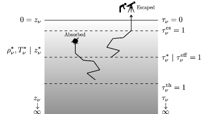
Refer to caption
Figure 6: Cartoon explaining the modified blackbody spectrum emerging from an optically thick, semi-infinite, plane-parallel, emitting atmosphere with total absorptive opacity ΞΊΞ½thsuperscriptsubscriptπœ…πœˆth\kappa_{\nu}^{\rm th}, but dominated by isotropic, coherent electron scattering opacities ΞΊΞ½es≫κνthmuch-greater-thansuperscriptsubscriptπœ…πœˆessuperscriptsubscriptπœ…πœˆth\kappa_{\nu}^{\rm es}\gg\kappa_{\nu}^{\rm th} in the non-relativistic limit (k​Teβ‰ͺme​c2much-less-thanπ‘˜subscript𝑇esubscriptπ‘šesuperscript𝑐2kT_{\rm e}\ll m_{\rm e}c^{2}; h​νβ‰ͺme​c2much-less-thanβ„Žπœˆsubscriptπ‘šesuperscript𝑐2h\nu\ll m_{\rm e}c^{2}). At the altitude zΞ½βˆ—superscriptsubscriptπ‘§πœˆβˆ—z_{\nu}^{\ast} of the effective photosphere, defined by where the effective β€œoptical depth” τνeffβ‰‘βˆ’βˆ«zΞ½βˆ—0[3​κνth​(ΞΊΞ½th+ΞΊΞ½es)]1/2​ρ​𝑑z=1superscriptsubscript𝜏𝜈effsuperscriptsubscriptsuperscriptsubscriptπ‘§πœˆβˆ—0superscriptdelimited-[]3superscriptsubscriptπœ…πœˆthsuperscriptsubscriptπœ…πœˆthsuperscriptsubscriptπœ…πœˆes12𝜌differential-d𝑧1\tau_{\nu}^{\rm eff}\equiv-\int_{z_{\nu}^{\ast}}^{0}[3\kappa_{\nu}^{\rm th}(\kappa_{\nu}^{\rm th}+\kappa_{\nu}^{\rm es})]^{1/2}\rho dz=1, the radiation gets thermalized with the gas temperature TΞ½βˆ—superscriptsubscriptπ‘‡πœˆβˆ—T_{\nu}^{\ast}. That is, a typical photon experiences its last absorption event at zΞ½βˆ—superscriptsubscriptπ‘§πœˆβˆ—z_{\nu}^{\ast}. Above zΞ½βˆ—superscriptsubscriptπ‘§πœˆβˆ—z_{\nu}^{\ast}, the radiation performs a scattering random walk to escape the atmosphere. The actual optical depth to the effective photosphere is Ο„Ξ½βˆ—=βˆ’βˆ«zΞ½βˆ—0(ΞΊΞ½th+ΞΊΞ½es)​ρ​𝑑z≫1superscriptsubscriptπœπœˆβˆ—superscriptsubscriptsuperscriptsubscriptπ‘§πœˆβˆ—0superscriptsubscriptπœ…πœˆthsuperscriptsubscriptπœ…πœˆes𝜌differential-d𝑧much-greater-than1\tau_{\nu}^{\ast}=-\int_{z_{\nu}^{\ast}}^{0}(\kappa_{\nu}^{\rm th}+\kappa_{\nu}^{\rm es})\rho dz\gg 1, so we assume thermal equilibrium there and Kirchoff’s law gives the emission coefficient at the effective photosphere, jΞ½thβ£βˆ—=ΞΊΞ½thβ£βˆ—β€‹ΟΞ½βˆ—β€‹Bν​(TΞ½βˆ—)superscriptsubscriptπ‘—πœˆthβˆ—superscriptsubscriptπœ…πœˆthβˆ—superscriptsubscriptπœŒπœˆβˆ—subscript𝐡𝜈superscriptsubscriptπ‘‡πœˆβˆ—j_{\nu}^{{\rm th}\ast}=\kappa_{\nu}^{{\rm th}\ast}\rho_{\nu}^{\ast}B_{\nu}(T_{\nu}^{\ast}). Absorption is not important above zΞ½βˆ—superscriptsubscriptπ‘§πœˆβˆ—z_{\nu}^{\ast}, so the radiative transfer equation for emission only gives the approximate emergent specific intensity Iν∼jΞ½thβ£βˆ—β€‹zΞ½βˆ—similar-tosubscript𝐼𝜈superscriptsubscriptπ‘—πœˆthβˆ—superscriptsubscriptπ‘§πœˆβˆ—I_{\nu}\sim j_{\nu}^{{\rm th}\ast}z_{\nu}^{\ast}. The modified blackbody of equation (A1) then follows, given jΞ½thβ£βˆ—superscriptsubscriptπ‘—πœˆthβˆ—j_{\nu}^{{\rm th}\ast} along with ΟΞ½βˆ—β€‹zΞ½βˆ—superscriptsubscriptπœŒπœˆβˆ—superscriptsubscriptπ‘§πœˆβˆ—\rho_{\nu}^{\ast}z_{\nu}^{\ast} from solving the approximation τνeff=1∼κνthβ£βˆ—β€‹ΞΊΞ½esβ£βˆ—β€‹ΟΞ½βˆ—β€‹zΞ½βˆ—superscriptsubscript𝜏𝜈eff1similar-tosuperscriptsubscriptπœ…πœˆthβˆ—superscriptsubscriptπœ…πœˆesβˆ—superscriptsubscriptπœŒπœˆβˆ—superscriptsubscriptπ‘§πœˆβˆ—\tau_{\nu}^{\rm eff}=1\sim\sqrt{\kappa_{\nu}^{{\rm th}\ast}\kappa_{\nu}^{{\rm es}\ast}}\rho_{\nu}^{\ast}z_{\nu}^{\ast}. The cartoon also marks the locations of the scattering-only photosphere τνes=1superscriptsubscript𝜏𝜈es1\tau_{\nu}^{\rm es}=1 and the absorption-only photosphere τνth=1superscriptsubscript𝜏𝜈th1\tau_{\nu}^{\rm th}=1. If Comptonization is saturated at the effective photosphere (yΞ½βˆ—β‰«1much-greater-thansuperscriptsubscriptπ‘¦πœˆβˆ—1y_{\nu}^{\ast}\gg 1), then thermalization occurs at the location where yΞ½=1subscriptπ‘¦πœˆ1y_{\nu}=1 rather than where τνeff=1superscriptsubscript𝜏𝜈eff1\tau_{\nu}^{\rm eff}=1.

Considering radiative diffusion as the only heat transport mechanism, the outgoing bolometric radiative flux is F=c​(d​Prad/d​τ)𝐹𝑐𝑑subscript𝑃radπ‘‘πœF=c(dP_{\rm rad}/d\tau). We assume that any flux added above the effective photosphere is small compared to the flux at the effective photosphere (i.e., F≃constantsimilar-to-or-equals𝐹constantF\simeq{\rm constant}). This amounts to the assumption that the energy dissipation rate per unit volume Ο΅=d​F/d​zitalic-ϡ𝑑𝐹𝑑𝑧\epsilon=dF/dz, or the volume-specific dissipation of accretion power, is negligible above the effective photosphere compared to all greater depths.202020Turbulence generated by the magneto-rotational instability, and presumably its associated dissipation, peaks above the mid-plane in the disc surface layers (e.g., Zhu & Stone, 2018), which if above the effective photosphere would nullify this F≃constantsimilar-to-or-equals𝐹constantF\simeq{\rm constant} assumption. Next, assuming local thermodynamic equilibrium (LTE) means the radiation pressure Pradβˆ—=(4​σ/3​c)​Tβˆ—4superscriptsubscript𝑃radβˆ—4𝜎3𝑐superscriptsubscriptπ‘‡βˆ—4P_{\rm rad}^{\ast}=(4\sigma/3c)T_{\ast}^{4} at the effective photosphere, and integrating the radiative diffusion equation from Ο„=0𝜏0\tau=0 down to the depth of formation Ο„=Ο„βˆ—πœsubscriptπœβˆ—\tau=\tau_{\ast} gives FβˆΌΟƒβ€‹Tβˆ—4/Ο„βˆ—similar-to𝐹𝜎superscriptsubscriptπ‘‡βˆ—4subscriptπœβˆ—F\sim\sigma T_{\ast}^{4}/\tau_{\ast}. Equating this expression to the definition of the effective temperature F≑σ​Teff4𝐹𝜎superscriptsubscript𝑇eff4F\equiv\sigma T_{\rm eff}^{4} (recall Ο„βˆ—β‰«1much-greater-thansubscriptπœβˆ—1\tau_{\ast}\gg 1) gives Tβˆ—βˆΌΟ„βˆ—1/4​Teffsimilar-tosubscriptπ‘‡βˆ—superscriptsubscriptπœβˆ—14subscript𝑇effT_{\ast}\sim\tau_{\ast}^{1/4}T_{\rm eff}. Substituting212121This comes from electron scattering being the dominant opacity source, such that Ο„βˆ—β‰ƒΟ„esβˆ—βˆΌΞΊesβˆ—β€‹Οβˆ—β€‹zβˆ—similar-to-or-equalssubscriptπœβˆ—superscriptsubscript𝜏esβˆ—similar-tosuperscriptsubscriptπœ…esβˆ—subscriptπœŒβˆ—subscriptπ‘§βˆ—\tau_{\ast}\simeq\tau_{\rm es}^{\ast}\sim\kappa_{\rm es}^{\ast}\rho_{\ast}z_{\ast}, combined with the approximation Ο„eff=1∼κthβˆ—β€‹ΞΊesβˆ—β€‹Οβˆ—β€‹zβˆ—subscript𝜏eff1similar-tosuperscriptsubscriptπœ…thβˆ—superscriptsubscriptπœ…esβˆ—subscriptπœŒβˆ—subscriptπ‘§βˆ—\tau_{\rm eff}=1\sim\sqrt{\kappa_{\rm th}^{\ast}\kappa_{\rm es}^{\ast}}\rho_{\ast}z_{\ast} (see Figure 6 caption). Ο„βˆ—βˆΌΞΊesβˆ—/ΞΊthβˆ—similar-tosubscriptπœβˆ—superscriptsubscriptπœ…esβˆ—superscriptsubscriptπœ…thβˆ—\tau_{\ast}\sim\sqrt{\kappa_{\rm es}^{\ast}/\kappa_{\rm th}^{\ast}} and recalling that ΞΊesβˆ—β‰«ΞΊthβˆ—much-greater-thansuperscriptsubscriptπœ…esβˆ—superscriptsubscriptπœ…thβˆ—\kappa_{\rm es}^{\ast}\gg\kappa_{\rm th}^{\ast}, we find the temperature at the effective photosphere Tβˆ—subscriptπ‘‡βˆ—T_{\ast} is ∼(ΞΊesβˆ—/ΞΊthβˆ—)1/8similar-toabsentsuperscriptsuperscriptsubscriptπœ…esβˆ—superscriptsubscriptπœ…thβˆ—18\sim(\kappa_{\rm es}^{\ast}/\kappa_{\rm th}^{\ast})^{1/8} times hotter than the effective temperature Teffsubscript𝑇effT_{\rm eff}, which means Bν​(Tβˆ—)subscript𝐡𝜈subscriptπ‘‡βˆ—B_{\nu}(T_{\ast}) in equation (A1) is spectrally harder than Bν​(Teff)subscript𝐡𝜈subscript𝑇effB_{\nu}(T_{\rm eff}).

Noticing that the (grey) dilution factor ΞΊthβˆ—/ΞΊesβˆ—superscriptsubscriptπœ…thβˆ—superscriptsubscriptπœ…esβˆ—\sqrt{\kappa_{\rm th}^{\ast}/\kappa_{\rm es}^{\ast}} is the minus fourth power of the hardening factor (ΞΊesβˆ—/ΞΊthβˆ—)1/8superscriptsuperscriptsubscriptπœ…esβˆ—superscriptsubscriptπœ…thβˆ—18(\kappa_{\rm es}^{\ast}/\kappa_{\rm th}^{\ast})^{1/8} motivates re-expressing equation (A1) as a colour-corrected blackbody (e.g., Shimura & Takahara, 1995)

IΞ½=1fcol4​Bν​(fcol​Teff),subscript𝐼𝜈1superscriptsubscript𝑓col4subscript𝐡𝜈subscript𝑓colsubscript𝑇effI_{\nu}=\frac{1}{f_{\rm col}^{4}}B_{\nu}\left(f_{\rm col}T_{\rm eff}\right), (A2)

where the colour correction factor fcol∼(ΞΊesβˆ—/ΞΊthβˆ—)1/8similar-tosubscript𝑓colsuperscriptsuperscriptsubscriptπœ…esβˆ—superscriptsubscriptπœ…thβˆ—18f_{\rm col}\sim(\kappa_{\rm es}^{\ast}/\kappa_{\rm th}^{\ast})^{1/8} phenomenologically relates the theoretically predicted effective temperature to the observed colour temperature Tcol=fcol​Teffsubscript𝑇colsubscript𝑓colsubscript𝑇effT_{\rm col}=f_{\rm col}T_{\rm eff}. The interpretation of fcolsubscript𝑓colf_{\rm col} is the multiplicative shift factor of spectral features to higher energies, while the fcolβˆ’4superscriptsubscript𝑓col4f_{\rm col}^{-4} factor out front keeps the ν​Iν𝜈subscript𝐼𝜈\nu I_{\nu} amplitude, and therefore the frequency-integrated intensity, constant (e.g., Davis & El-Abd, 2019). The colour-corrected blackbody approximation of equation (A2) neglects the frequency-dependence of thermalization. In general, the frequency-dependence of the depth of formation Ο„Ξ½βˆ—superscriptsubscriptπœπœˆβˆ—\tau_{\nu}^{\ast} and the location where the Compton y𝑦y-parameter yΞ½=1subscriptπ‘¦πœˆ1y_{\nu}=1 means that different frequencies probe different atmospheric depths and therefore different temperatures. Assessing the applicability of the colour-corrected blackbody approximation to accretion disc spectra requires sophisticated modeling.

The modified blackbody arises when electron scattering is an important opacity source, but spectral hardening is also sensitive to the profile of gas temperature, which generally decreases at higher disc altitudes. When the effective photosphere (i.e., where escaping radiation gets thermalized with the gas) is deeper in the atmosphere, the thermalization temperature Tβˆ—subscriptπ‘‡βˆ—T_{\ast} is hotter and so the emergent spectrum is harder. Adding bound-free opacities increases the total absorptive opacity ΞΊthsubscriptπœ…th\kappa_{\rm th}, which pushes the effective photosphere to higher disc altitudes where Tβˆ—subscriptπ‘‡βˆ—T_{\ast} is colder, making the emergent modified blackbody softer. Adding bound-free opacities reduces the ratio of scattering-to-absorption opacities ΞΊes/ΞΊthsubscriptπœ…essubscriptπœ…th\kappa_{\rm es}/\kappa_{\rm th}, which also softens the emergent spectrum. These two effects might explain why fcolsubscript𝑓colf_{\rm col} is slightly lower when bound-free absorption opacities are included (Davis etΒ al., 2005), compared to considering only free-free absorption opacities (Shimura & Takahara, 1995).

Finally, there is the question of what physical process is responsible for thermalizing the radiation? The preceding discussion supposes that absorption dictates thermalization, but thermalization with the non-relativistic electrons is possible for saturated Comptonization; that is, when the Compton y𝑦y-parameter at the effective photosphere yΞ½βˆ—β‰‘4​kB​TΞ½βˆ—/(me​c2)​max⁑(Ο„Ξ½βˆ—2,Ο„Ξ½βˆ—)superscriptsubscriptπ‘¦πœˆβˆ—4subscriptπ‘˜Bsuperscriptsubscriptπ‘‡πœˆβˆ—subscriptπ‘šesuperscript𝑐2superscriptsubscriptπœπœˆβˆ—absent2superscriptsubscriptπœπœˆβˆ—y_{\nu}^{\ast}\equiv 4k_{\rm B}T_{\nu}^{\ast}/(m_{\rm e}c^{2})\max(\tau_{\nu}^{\ast 2},\tau_{\nu}^{\ast}) is large (yΞ½βˆ—β‰«1much-greater-thansuperscriptsubscriptπ‘¦πœˆβˆ—1y_{\nu}^{\ast}\gg 1). In this scenario, the blackbody spectrum Bν​(TΞ½βˆ—)subscript𝐡𝜈superscriptsubscriptπ‘‡πœˆβˆ—B_{\nu}(T_{\nu}^{\ast}) produced at the effective photosphere diffuses outward and continually experiences incoherent Compton (down)scattering, ultimately emerging as a softer, Wien-like spectrum with a temperature corresponding to the altitude where y≃1similar-to-or-equals𝑦1y\simeq 1 (Ross etΒ al., 1992). Early models neglecting bound-free opacities showed saturated Comptonization (yΞ½βˆ—β‰«1much-greater-thansuperscriptsubscriptπ‘¦πœˆβˆ—1y_{\nu}^{\ast}\gg 1) and found that a colour-corrected disc blackbody well-approximated the emergent disc continuum for luminosities l≳0.01greater-than-or-equivalent-to𝑙0.01l\gtrsim 0.01 (Shimura & Takahara, 1995). These models found that disc annuli with yΞ½βˆ—β‰«1much-greater-thansuperscriptsubscriptπ‘¦πœˆβˆ—1y_{\nu}^{\ast}\gg 1 were better approximated by a colour-corrected blackbody than their yΞ½βˆ—β‰ͺ1much-less-thansuperscriptsubscriptπ‘¦πœˆβˆ—1y_{\nu}^{\ast}\ll 1 counterparts, and attributed this improvement to Comptonization providing enhanced thermalization of the radiation with the gas. More recent models including bound-free opacities showed Comptonization to be much less important (yΞ½βˆ—β‰²1less-than-or-similar-tosuperscriptsubscriptπ‘¦πœˆβˆ—1y_{\nu}^{\ast}\lesssim 1), but still found that a colour-corrected disc blackbody well-approximated the emergent disc continuum (Davis etΒ al., 2005). This success was attributed to the relative frequency-independence of Ο„Ξ½βˆ—superscriptsubscriptπœπœˆβˆ—\tau_{\nu}^{\ast}, such that photons with different frequencies probe similar temperatures because thermalization occurs over a confined range of atmospheric depths.

Appendix B Accretion Disc Continuum Model

Our starting point is the observed specific disc flux calculated from the kerrbb model (equation E2 of Li etΒ al., 2005),

FEobs=∫g3​IEem​𝑑Ωobs,subscript𝐹subscript𝐸obssuperscript𝑔3subscript𝐼subscript𝐸emdifferential-dsubscriptΞ©obsF_{E_{\rm obs}}=\int g^{3}I_{E_{\rm em}}d\Omega_{\rm obs}, (B1)

which accounts for relativistic effects on photon propagation from the disc surface to the observer by using a ray-tracing technique. Here, IEemsubscript𝐼subscript𝐸emI_{E_{\rm em}} is the specific intensity emitted from the disc surface, Eobssubscript𝐸obsE_{\rm obs} is the observed photon energy, and g≑Eobs/Eem𝑔subscript𝐸obssubscript𝐸emg\equiv E_{\rm obs}/E_{\rm em} is the redshift factor relating the observed and emitted photon energies. The solid angle element of the disc image plane seen by the observer, but written in terms of polar coordinates in the disc equatorial plane, is d​Ωobs=R​d​R​d​ϕ​cos⁑(idisc)/D2𝑑subscriptΞ©obs𝑅𝑑𝑅𝑑italic-Ο•subscript𝑖discsuperscript𝐷2d\Omega_{\rm obs}=R~{}dR~{}d\phi~{}\cos(i_{\rm disc})/D^{2}. Assuming IEemsubscript𝐼subscript𝐸emI_{E_{\rm em}} obeys a colour-corrected blackbody spectrum according to the local disc colour temperature Tcol​(R)=fcol​Teff​(R)subscript𝑇col𝑅subscript𝑓colsubscript𝑇eff𝑅T_{\rm col}(R)=f_{\rm col}T_{\rm eff}(R), equation (B1) becomes (equation E7 of Li etΒ al., 2005)

FEobs=1fcol4​2​Eobs3h3​c2β€‹βˆ«[exp⁑(Eobsg​kB​Tcol​(R))βˆ’1]βˆ’1​Ξ₯​(ΞΈ)​𝑑Ωobs,subscript𝐹subscript𝐸obs1superscriptsubscript𝑓col42superscriptsubscript𝐸obs3superscriptβ„Ž3superscript𝑐2superscriptdelimited-[]subscript𝐸obs𝑔subscriptπ‘˜Bsubscript𝑇col𝑅11Ξ₯πœƒdifferential-dsubscriptΞ©obsF_{E_{\rm obs}}=\frac{1}{f_{\rm col}^{4}}\frac{2E_{\rm obs}^{3}}{h^{3}c^{2}}\int\left[\exp\left(\frac{E_{\rm obs}}{gk_{\rm B}T_{\rm col}\left(R\right)}\right)-1\right]^{-1}\Upsilon\left(\theta\right)d\Omega_{\rm obs}, (B2)

where the colour correction factor fcolsubscript𝑓colf_{\rm col} (assumed to be constant) relates the colour and effective temperatures. The kerrbb model obtains Teff​(R)=[Fout​(R)/ΟƒSB]1/4subscript𝑇eff𝑅superscriptdelimited-[]subscript𝐹out𝑅subscript𝜎SB14T_{\rm eff}(R)=[F_{\rm out}(R)/\sigma_{\rm SB}]^{1/4} by calculating the outgoing flux Foutsubscript𝐹outF_{\rm out} through an iterative procedure that uses the aforementioned ray-tracing technique. The limb-darkening law describing the angular distribution of IEemsubscript𝐼subscript𝐸emI_{E_{\rm em}} is taken to be that of a plane-parallel, semi-infinite, electron scattering atmosphere (Chandrasekhar, 1960; Fukue & Akizuki, 2006),

Ξ₯​(ΞΈ)=12+34​cos⁑(ΞΈ),Ξ₯πœƒ1234πœƒ\Upsilon\left(\theta\right)=\frac{1}{2}+\frac{3}{4}\cos\left(\theta\right), (B3)

where ΞΈπœƒ\theta is the polar angle measured from the disc surface normal to the wavevector of the emitted photon. Defining r~≑R/Rin~π‘Ÿπ‘…subscript𝑅in\tilde{r}\equiv R/R_{\rm in} as the radial coordinate in units of the inner disc radius Rinsubscript𝑅inR_{\rm in} and performing the change of variables Rβ†’r~→𝑅~π‘ŸR\rightarrow\tilde{r}, equation (B2) becomes

FEobs=rin2fcol4​(G​M/c2D)2​cos⁑(idisc)​2​Eobs3h3​c2β€‹βˆ«02β€‹Ο€βˆ«1r~out[exp⁑(Eobsg​kB​Tcol​(r~))βˆ’1]βˆ’1​Ξ₯​(ΞΈ)​r~​𝑑r~​𝑑ϕ,subscript𝐹subscript𝐸obssuperscriptsubscriptπ‘Ÿin2superscriptsubscript𝑓col4superscript𝐺𝑀superscript𝑐2𝐷2subscript𝑖disc2superscriptsubscript𝐸obs3superscriptβ„Ž3superscript𝑐2superscriptsubscript02πœ‹superscriptsubscript1subscript~π‘Ÿoutsuperscriptdelimited-[]subscript𝐸obs𝑔subscriptπ‘˜Bsubscript𝑇col~π‘Ÿ11Ξ₯πœƒ~π‘Ÿdifferential-d~π‘Ÿdifferential-ditalic-Ο•F_{E_{\rm obs}}=\frac{r_{\rm in}^{2}}{f_{\rm col}^{4}}\left(\frac{GM/c^{2}}{D}\right)^{2}\cos\left(i_{\rm disc}\right)\frac{2E_{\rm obs}^{3}}{h^{3}c^{2}}\int\limits_{0}^{2\pi}\int\limits_{1}^{\tilde{r}_{\rm out}}\left[\exp\left(\frac{E_{\rm obs}}{gk_{\rm B}T_{\rm col}\left(\tilde{r}\right)}\right)-1\right]^{-1}\Upsilon\left(\theta\right)\tilde{r}~{}d\tilde{r}~{}d\phi, (B4)

where (no tilde) r≑R/Rgπ‘Ÿπ‘…subscript𝑅gr\equiv R/R_{\rm g} is the radial coordinate in units of the gravitational radius Rg=G​M/c2subscript𝑅g𝐺𝑀superscript𝑐2R_{\rm g}=GM/c^{2}. The dependence of the disc continuum model on the system parameters {rin,fcol,M,D,idisc}subscriptπ‘Ÿinsubscript𝑓col𝑀𝐷subscript𝑖disc\{r_{\rm in},f_{\rm col},M,D,i_{\rm disc}\} is now apparent and a dependence on the mass accretion rate M˙˙𝑀\dot{M} is contained within Tcolsubscript𝑇colT_{\rm col}. Integrating FEobssubscript𝐹subscript𝐸obsF_{E_{\rm obs}} over Eobssubscript𝐸obsE_{\rm obs} then gives the total observed disc flux,

Fobs=∫0∞FEobs​𝑑Eobs.subscript𝐹obssuperscriptsubscript0subscript𝐹subscript𝐸obsdifferential-dsubscript𝐸obsF_{\rm obs}=\int\limits_{0}^{\infty}F_{E_{\rm obs}}dE_{\rm obs}. (B5)

Our first objective is to find an equivalent expression for Fobssubscript𝐹obsF_{\rm obs} that replaces the integral in equation (B4) with something more tractable (i.e., that does not require ray tracing). We will achieve this by isolating the relativistic effects on photon propagation into β€œdisc flux correction factors,” as follows. Ignoring relativistic effects on photon propagation (as indicated by the ^^absent\widehat{\;} symbol below) means that the outgoing flux is axisymmetric, the photons experience no redshift (g=1𝑔1g=1), and only the photons emitted from the disc surface with polar angle ΞΈ=idiscπœƒsubscript𝑖disc\theta=i_{\rm disc} reach the observer. The total observed disc flux that results from this simplification is (e.g., Mitsuda etΒ al., 1984; Zimmerman etΒ al., 2005)

F^obs=rin2fcol4​(G​M/c2D)2​cos⁑(idisc)​Ξ₯​(idisc)β€‹βˆ«0∞4​π​Eobs3h3​c2β€‹βˆ«1r~out[exp⁑(EobskB​Tcol​(r~))βˆ’1]βˆ’1​r~​𝑑r~​𝑑Eobs.subscript^𝐹obssuperscriptsubscriptπ‘Ÿin2superscriptsubscript𝑓col4superscript𝐺𝑀superscript𝑐2𝐷2subscript𝑖discΞ₯subscript𝑖discsuperscriptsubscript04πœ‹superscriptsubscript𝐸obs3superscriptβ„Ž3superscript𝑐2superscriptsubscript1subscript~π‘Ÿoutsuperscriptdelimited-[]subscript𝐸obssubscriptπ‘˜Bsubscript𝑇col~π‘Ÿ11~π‘Ÿdifferential-d~π‘Ÿdifferential-dsubscript𝐸obs\widehat{F}_{\rm obs}=\frac{r_{\rm in}^{2}}{f_{\rm col}^{4}}\left(\frac{GM/c^{2}}{D}\right)^{2}\cos\left(i_{\rm disc}\right)\Upsilon\left(i_{\rm disc}\right)\int\limits_{0}^{\infty}\frac{4\pi E_{\rm obs}^{3}}{h^{3}c^{2}}\int\limits_{1}^{\tilde{r}_{\rm out}}\left[\exp\left(\frac{E_{\rm obs}}{k_{\rm B}T_{\rm col}\left(\tilde{r}\right)}\right)-1\right]^{-1}\tilde{r}~{}d\tilde{r}~{}dE_{\rm obs}. (B6)

To isolate the effect of neglecting relativistic photon propagation on the total observed disc flux, we must adopt the same underlying disc physics used by the kerrbb model; that is, the standard relativistic β€œΞ±π›Ό\alpha-disc” model for a geometrically thin, optically thick accretion disc. The α𝛼\alpha-disc model predicts the radial profile of the colour temperature at the disc mid-plane to be (Shakura & Sunyaev, 1973)

Tcol​(x)=fcol​[3​G​M​MΛ™8​π​σSB​Rg3​f​(x)]1/4,subscript𝑇colπ‘₯subscript𝑓colsuperscriptdelimited-[]3𝐺𝑀˙𝑀8πœ‹subscript𝜎SBsuperscriptsubscript𝑅g3𝑓π‘₯14T_{\rm col}(x)=f_{\rm col}\left[\frac{3GM\dot{M}}{8\pi\sigma_{\rm SB}R_{\rm g}^{3}}f\left(x\right)\right]^{1/4}, (B7)

where the radial coordinate is parametrized as x≑(R/Rg)1/2=(r~​Rin/Rg)1/2π‘₯superscript𝑅subscript𝑅g12superscript~π‘Ÿsubscript𝑅insubscript𝑅g12x\equiv(R/R_{\rm g})^{1/2}=(\tilde{r}R_{\rm in}/R_{\rm g})^{1/2} and f​(x)𝑓π‘₯f(x) describes the radial profile of gravitational energy released in the form of a radiation flux through the disc surfaces. The time-steady mass accretion rate M˙˙𝑀\dot{M} through the disc is taken to be radially independent and one generally assumes a zero-torque boundary condition on the inner disc edge. With these assumptions, the relativistic radial disc structure adopted by kerrbb gives f​(x)𝑓π‘₯f(x) as (Novikov & Thorne, 1973; Page & Thorne, 1974)

fNT​(x)subscript𝑓NTπ‘₯\displaystyle f_{\rm NT}\left(x\right) =1x4​(x3βˆ’3​x+2​a)[xβˆ’x0βˆ’32aln(xx0)βˆ’3​(x1βˆ’a)2x1​(x1βˆ’x2)​(x1βˆ’x3)ln(xβˆ’x1x0βˆ’x1)\displaystyle=\frac{1}{x^{4}\left(x^{3}-3x+2a\right)}\left[x-x_{0}-\frac{3}{2}a\ln\left(\frac{x}{x_{0}}\right)-\frac{3\left(x_{1}-a\right)^{2}}{x_{1}\left(x_{1}-x_{2}\right)\left(x_{1}-x_{3}\right)}\ln\left(\frac{x-x_{1}}{x_{0}-x_{1}}\right)\right.
βˆ’3​(x2βˆ’a)2x2​(x2βˆ’x1)​(x2βˆ’x3)ln(xβˆ’x2x0βˆ’x2)βˆ’3​(x3βˆ’a)2x3​(x3βˆ’x1)​(x3βˆ’x2)ln(xβˆ’x3x0βˆ’x3)],\displaystyle\left.-\frac{3\left(x_{2}-a\right)^{2}}{x_{2}\left(x_{2}-x_{1}\right)\left(x_{2}-x_{3}\right)}\ln\left(\frac{x-x_{2}}{x_{0}-x_{2}}\right)-\frac{3\left(x_{3}-a\right)^{2}}{x_{3}\left(x_{3}-x_{1}\right)\left(x_{3}-x_{2}\right)}\ln\left(\frac{x-x_{3}}{x_{0}-x_{3}}\right)\right], (B8)

where,

x0≑(RinRg)1/2,x1≑2​cos⁑(13​cosβˆ’1⁑(a)βˆ’Ο€3),x2≑2​cos⁑(13​cosβˆ’1⁑(a)+Ο€3),x3β‰‘βˆ’2​cos⁑(13​cosβˆ’1⁑(a)),formulae-sequencesubscriptπ‘₯0superscriptsubscript𝑅insubscript𝑅g12formulae-sequencesubscriptπ‘₯1213superscript1π‘Žπœ‹3formulae-sequencesubscriptπ‘₯2213superscript1π‘Žπœ‹3subscriptπ‘₯3213superscript1π‘Žx_{0}\equiv\left(\frac{R_{\rm in}}{R_{\rm g}}\right)^{1/2},\qquad x_{1}\equiv 2\cos\left(\frac{1}{3}\cos^{-1}\left(a\right)-\frac{\pi}{3}\right),\qquad x_{2}\equiv 2\cos\left(\frac{1}{3}\cos^{-1}\left(a\right)+\frac{\pi}{3}\right),\qquad x_{3}\equiv-2\cos\left(\frac{1}{3}\cos^{-1}\left(a\right)\right), (B9)

and a=J/(Rg​M​c)π‘Žπ½subscript𝑅g𝑀𝑐a=J/(R_{\rm g}Mc) is the black hole spin parameter, where J𝐽J is the black hole angular momentum. The black hole spin is interchangeable with the inner disc radius under the standard assumption that rinsubscriptπ‘Ÿinr_{\rm in} coincides with the location of the innermost stable circular orbit (ISCO), which depends on aπ‘Ža monotonically (Bardeen etΒ al., 1972),

rISCO={3+Z2βˆ’(3βˆ’Z1)​(3+Z1+2​Z2),for0≀a≀+13+Z2+(3βˆ’Z1)​(3+Z1+2​Z2),forβˆ’1≀a<0,r_{\rm ISCO}=\left\{\begin{array}[]{@{\hspace{0mm}}l@{\hspace{1mm}}l@{\hspace{0mm}}}3+Z_{2}-\sqrt{\left(3-Z_{1}\right)\left(3+Z_{1}+2Z_{2}\right)}\hfil\hskip 2.84526pt&,~{}\mathrm{for}~{}0\leq a\leq+1\\ \hfil\hskip 2.84526pt\\ 3+Z_{2}+\sqrt{\left(3-Z_{1}\right)\left(3+Z_{1}+2Z_{2}\right)}\hfil\hskip 2.84526pt&,~{}\mathrm{for}~{}-1\leq a<0,\end{array}\right. (B10)

where,

Z1≑1+(1βˆ’a2)1/3​[(1+a)1/3+(1βˆ’a)1/3],Z2≑3​a2+Z12.formulae-sequencesubscript𝑍11superscript1superscriptπ‘Ž213delimited-[]superscript1π‘Ž13superscript1π‘Ž13subscript𝑍23superscriptπ‘Ž2superscriptsubscript𝑍12Z_{1}\equiv 1+\left(1-a^{2}\right)^{1/3}\left[\left(1+a\right)^{1/3}+\left(1-a\right)^{1/3}\right],\qquad Z_{2}\equiv\sqrt{3a^{2}+Z_{1}^{2}}. (B11)

For a set of model parameters {rin,fcol,M,D,idisc,MΛ™}subscriptπ‘Ÿinsubscript𝑓col𝑀𝐷subscript𝑖disc˙𝑀\{r_{\rm in},f_{\rm col},M,D,i_{\rm disc},\dot{M}\}, we can calculate F^obssubscript^𝐹obs\widehat{F}_{\rm obs} from equation (B6), given Tcol​(r~)subscript𝑇col~π‘ŸT_{\rm col}(\tilde{r}) as determined by inserting an explicit expression for f​(x)𝑓π‘₯f(x) in equation (B7). Choosing the relativistic radial disc structure fNT​(x)subscript𝑓NTπ‘₯f_{\rm NT}(x) from equation (B8) defines the radial profile of the colour temperature TcolNT​(x)superscriptsubscript𝑇colNTπ‘₯T_{\rm col}^{\rm NT}(x), which we insert into equation (B6) to obtain the corresponding total observed disc flux F^obsNTsuperscriptsubscript^𝐹obsNT\widehat{F}_{\rm obs}^{\rm NT}. Because F^obsNTsuperscriptsubscript^𝐹obsNT\widehat{F}_{\rm obs}^{\rm NT} and Fobssubscript𝐹obsF_{\rm obs} have identical temperature profiles, they only differ in their treatment of relativistic effects on photon propagation, which F^obsNTsuperscriptsubscript^𝐹obsNT\widehat{F}_{\rm obs}^{\rm NT} ignores and Fobssubscript𝐹obsF_{\rm obs} includes. To isolate these effects on the total observed disc flux, we define the disc flux correction factor (e.g., Cunningham, 1975; Zhang etΒ al., 1997)

gGR​(rin,idisc)=FobsF^obsNT,subscript𝑔GRsubscriptπ‘Ÿinsubscript𝑖discsubscript𝐹obssuperscriptsubscript^𝐹obsNTg_{\rm GR}\left(r_{\rm in},i_{\rm disc}\right)=\frac{F_{\rm obs}}{\widehat{F}_{\rm obs}^{\rm NT}}, (B12)

which we tabulate in Β§B.1. Having condensed the relativistic effects on the propagation of photons from the disc surface to the observer into the correction factor gGR​(rin,idisc)subscript𝑔GRsubscriptπ‘Ÿinsubscript𝑖discg_{\rm GR}(r_{\rm in},i_{\rm disc}), equation (B5) becomes

Fobs=rin2fcol4​(G​M/c2D)2​cos⁑(idisc)​Ξ₯​(idisc)​gGR​(rin,idisc)β€‹βˆ«0∞4​π​Eobs3h3​c2β€‹βˆ«1r~out[exp⁑(EobskB​TcolNT​(r~))βˆ’1]βˆ’1​r~​𝑑r~​𝑑Eobs,subscript𝐹obssuperscriptsubscriptπ‘Ÿin2superscriptsubscript𝑓col4superscript𝐺𝑀superscript𝑐2𝐷2subscript𝑖discΞ₯subscript𝑖discsubscript𝑔GRsubscriptπ‘Ÿinsubscript𝑖discsuperscriptsubscript04πœ‹superscriptsubscript𝐸obs3superscriptβ„Ž3superscript𝑐2superscriptsubscript1subscript~π‘Ÿoutsuperscriptdelimited-[]subscript𝐸obssubscriptπ‘˜Bsuperscriptsubscript𝑇colNT~π‘Ÿ11~π‘Ÿdifferential-d~π‘Ÿdifferential-dsubscript𝐸obsF_{\rm obs}=\frac{r_{\rm in}^{2}}{f_{\rm col}^{4}}\left(\frac{GM/c^{2}}{D}\right)^{2}\cos\left(i_{\rm disc}\right)\Upsilon\left(i_{\rm disc}\right)g_{\rm GR}\left(r_{\rm in},i_{\rm disc}\right)\int\limits_{0}^{\infty}\frac{4\pi E_{\rm obs}^{3}}{h^{3}c^{2}}\int\limits_{1}^{\tilde{r}_{\rm out}}\left[\exp\left(\frac{E_{\rm obs}}{k_{\rm B}T_{\rm col}^{\rm NT}\left(\tilde{r}\right)}\right)-1\right]^{-1}\tilde{r}~{}d\tilde{r}~{}dE_{\rm obs}, (B13)

which is equivalent to Fobssubscript𝐹obsF_{\rm obs} calculated using kerrbb. Notably, we took advantage of the kerrbb ray-tracing calculations by pre-computing gGRsubscript𝑔GRg_{\rm GR}, such that we can calculate Fobssubscript𝐹obsF_{\rm obs} from equation (B13) with straightforward integration.

Our next objective is to reduce equation (B13) to a two-parameter disc model described by only a disc flux normalization and a characteristic colour temperature, just like the diskbb family of disc models (Mitsuda etΒ al., 1984). As equation (B13) currently stands, the factors outside the integrals could be rolled into a single β€œnormalization” model parameter, but parametrizing the colour temperature profile is more complicated. Notably, in the non-relativistic limit for the radial disc structure, we have f​(x)β†’fSS​(x)=(xβˆ’x0)/x7→𝑓π‘₯subscript𝑓SSπ‘₯π‘₯subscriptπ‘₯0superscriptπ‘₯7f(x)\rightarrow f_{\rm SS}(x)=(x-x_{0})/x^{7} and the corresponding colour temperature profile (Shakura & Sunyaev, 1973)

TcolSS​(r~)=Tcolβˆ—β€‹r~βˆ’3/4​(1βˆ’r~βˆ’1/2)1/4superscriptsubscript𝑇colSS~π‘Ÿsuperscriptsubscript𝑇colβˆ—superscript~π‘Ÿ34superscript1superscript~π‘Ÿ1214T_{\rm col}^{\rm SS}\left(\tilde{r}\right)=T_{\rm col}^{\ast}\tilde{r}^{-3/4}\left(1-\tilde{r}^{-1/2}\right)^{1/4} (B14)

is completely specified by the characteristic colour temperature (e.g., Frank etΒ al., 2002)

Tcolβˆ—β‰‘fcol​(3​G​M​MΛ™8​π​σSB​Rin3)1/4,superscriptsubscript𝑇colβˆ—subscript𝑓colsuperscript3𝐺𝑀˙𝑀8πœ‹subscript𝜎SBsuperscriptsubscript𝑅in314T_{\rm col}^{\ast}\equiv f_{\rm col}\left(\frac{3GM\dot{M}}{8\pi\sigma_{\rm SB}R_{\rm in}^{3}}\right)^{1/4}, (B15)

which allows equation (B13) to be reduced to a two-parameter model. However, unlike TcolSS​(r~)superscriptsubscript𝑇colSS~π‘ŸT_{\rm col}^{\rm SS}(\tilde{r}), the colour temperature profile TcolNT​(x)superscriptsubscript𝑇colNTπ‘₯T_{\rm col}^{\rm NT}(x) associated with the relativistic radial disc structure used by kerrbb cannot be parametrized in terms of only Tcolβˆ—superscriptsubscript𝑇colβˆ—T_{\rm col}^{\ast}, but also requires specifying rinsubscriptπ‘Ÿinr_{\rm in} because this sets the black hole spin aπ‘Ža (assuming rin=rISCOsubscriptπ‘Ÿinsubscriptπ‘ŸISCOr_{\rm in}=r_{\rm ISCO}) as needed by fNT​(x)subscript𝑓NTπ‘₯f_{\rm NT}(x). Analogously to our calculation of gGRsubscript𝑔GRg_{\rm GR} above, we can isolate the effects of a relativistic radial disc structure by defining another disc flux correction factor (tabulated in Β§B.1)

gNT​(rin)=F^obsNTF^obsSS,subscript𝑔NTsubscriptπ‘Ÿinsuperscriptsubscript^𝐹obsNTsuperscriptsubscript^𝐹obsSSg_{\rm NT}\left(r_{\rm in}\right)=\frac{\widehat{F}_{\rm obs}^{\rm NT}}{\widehat{F}_{\rm obs}^{\rm SS}}, (B16)

where we calculate F^obsSSsuperscriptsubscript^𝐹obsSS\widehat{F}_{\rm obs}^{\rm SS} using equation (B6), with TcolSS​(r~)superscriptsubscript𝑇colSS~π‘ŸT_{\rm col}^{\rm SS}(\tilde{r}) from equation (B14) inserted for Tcol​(r~)subscript𝑇col~π‘ŸT_{\rm col}(\tilde{r}). Condensing the relativistic effects on the radial profile of the colour temperature into the correction factor gNT​(rin)subscript𝑔NTsubscriptπ‘Ÿing_{\rm NT}(r_{\rm in}), we can write equation (B13) as a two-parameter β€” Kfluxsubscript𝐾fluxK_{\rm flux} and Tcolβˆ—superscriptsubscript𝑇colβˆ—T_{\rm col}^{\ast} β€” model for the total observed disc flux

Fobs=Kfluxβ€‹βˆ«0∞4​π​Eobs3h3​c2β€‹βˆ«1r~out[exp⁑(EobskB​Tcolβˆ—β€‹r~βˆ’3/4​(1βˆ’r~βˆ’1/2)1/4)βˆ’1]βˆ’1​r~​𝑑r~​𝑑Eobs,subscript𝐹obssubscript𝐾fluxsuperscriptsubscript04πœ‹superscriptsubscript𝐸obs3superscriptβ„Ž3superscript𝑐2superscriptsubscript1subscript~π‘Ÿoutsuperscriptdelimited-[]subscript𝐸obssubscriptπ‘˜Bsuperscriptsubscript𝑇colβˆ—superscript~π‘Ÿ34superscript1superscript~π‘Ÿ121411~π‘Ÿdifferential-d~π‘Ÿdifferential-dsubscript𝐸obsF_{\rm obs}=K_{\rm flux}\int\limits_{0}^{\infty}\frac{4\pi E_{\rm obs}^{3}}{h^{3}c^{2}}\int\limits_{1}^{\tilde{r}_{\rm out}}\left[\exp\left(\frac{E_{\rm obs}}{k_{\rm B}T_{\rm col}^{\ast}\tilde{r}^{-3/4}\left(1-\tilde{r}^{-1/2}\right)^{1/4}}\right)-1\right]^{-1}\tilde{r}~{}d\tilde{r}~{}dE_{\rm obs}, (B17)

where we combined {rin,fcol,M,D,idisc}subscriptπ‘Ÿinsubscript𝑓col𝑀𝐷subscript𝑖disc\{r_{\rm in},f_{\rm col},M,D,i_{\rm disc}\} into a single model parameter called the β€œdisc flux normalization”

Kflux≑rin2fcol4​(G​M/c2D)2​cos⁑(idisc)​Ξ₯​(idisc)​gGR​(rin,idisc)​gNT​(rin).subscript𝐾fluxsuperscriptsubscriptπ‘Ÿin2superscriptsubscript𝑓col4superscript𝐺𝑀superscript𝑐2𝐷2subscript𝑖discΞ₯subscript𝑖discsubscript𝑔GRsubscriptπ‘Ÿinsubscript𝑖discsubscript𝑔NTsubscriptπ‘ŸinK_{\rm flux}\equiv\frac{r_{\rm in}^{2}}{f_{\rm col}^{4}}\left(\frac{GM/c^{2}}{D}\right)^{2}\cos\left(i_{\rm disc}\right)\Upsilon\left(i_{\rm disc}\right)g_{\rm GR}\left(r_{\rm in},i_{\rm disc}\right)g_{\rm NT}\left(r_{\rm in}\right). (B18)

For the same set of input parameters {rin,fcol,M,D,idisc,MΛ™}subscriptπ‘Ÿinsubscript𝑓col𝑀𝐷subscript𝑖disc˙𝑀\{r_{\rm in},f_{\rm col},M,D,i_{\rm disc},\dot{M}\}, the total observed disc flux Fobssubscript𝐹obsF_{\rm obs} calculated from equation (B17) is identical to that calculated from the kerrbb model.
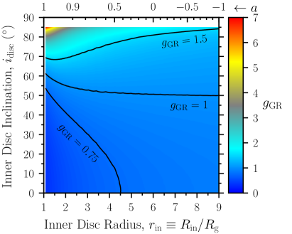
Refer to caption
Refer to caption
Figure 7: Left: Disc flux correction factor gGR​(rin,idisc)subscript𝑔GRsubscriptπ‘Ÿinsubscript𝑖discg_{\rm GR}(r_{\rm in},i_{\rm disc}), which accounts for relativistic effects on photon propagation, on a grid of inner disc radius rinsubscriptπ‘Ÿinr_{\rm in} and inner disc inclination angle idiscsubscript𝑖disci_{\rm disc}. The top xπ‘₯x-axis gives the black hole spin parameter aπ‘Ža corresponding to rinsubscriptπ‘Ÿinr_{\rm in}, assuming rin=rISCOsubscriptπ‘Ÿinsubscriptπ‘ŸISCOr_{\rm in}=r_{\rm ISCO}. Significant departures of gGRsubscript𝑔GRg_{\rm GR} away from unity occur for moderate-to-extreme prograde black hole spins and/or more edge-on disc inclinations. For a non-spinning black hole, gGR=1subscript𝑔GR1g_{\rm GR}=1 when idisc=50​.βˆ˜β€‹7subscript𝑖disc50degree7i_{\rm disc}=50\fdg 7. The gGRsubscript𝑔GRg_{\rm GR} extrema are [0.33,6.9]0.336.9[0.33,6.9]. White regions show the parameter space inaccessible to kerrbb. Right: Inner disc radius partial derivative of the disc flux correction factor βˆ‚gGR/βˆ‚rinsubscript𝑔GRsubscriptπ‘Ÿin\partial g_{\rm GR}/\partial r_{\rm in}, which is needed to compute the Jacobian determinant of equation (C14). The gGRsubscript𝑔GRg_{\rm GR} contour lines show artifacts (resembling ocean surface waves) that get amplified to large oscillations in βˆ‚gGR/βˆ‚rinsubscript𝑔GRsubscriptπ‘Ÿin\partial g_{\rm GR}/\partial r_{\rm in}, so we smoothed βˆ‚gGR/βˆ‚rinsubscript𝑔GRsubscriptπ‘Ÿin\partial g_{\rm GR}/\partial r_{\rm in} along the rinsubscriptπ‘Ÿinr_{\rm in}-dimension using a Gaussian filter, whose kernel required a standard deviation of 25​Rg25subscript𝑅g25~{}R_{\rm g} to yield the smooth, non-oscillatory contour lines shown in the plot. After smoothing, the βˆ‚gGR/βˆ‚rinsubscript𝑔GRsubscriptπ‘Ÿin\partial g_{\rm GR}/\partial r_{\rm in} extrema are [βˆ’3.1,1.3]3.11.3[-3.1,1.3].
Refer to caption
Figure 8: Disc flux correction factor gNT​(rin)subscript𝑔NTsubscriptπ‘Ÿing_{\rm NT}(r_{\rm in}) (left axis; solid blue line), which accounts for relativistic effects on the radial disc structure, and its derivative d​gNT/d​rin𝑑subscript𝑔NT𝑑subscriptπ‘Ÿindg_{\rm NT}/dr_{\rm in} (right axis; dashed orange line), which is needed to compute the Jacobian determinant of equation (C14). The top xπ‘₯x-axis gives the black hole spin parameter aπ‘Ža corresponding to rinsubscriptπ‘Ÿinr_{\rm in}, assuming rin=rISCOsubscriptπ‘Ÿinsubscriptπ‘ŸISCOr_{\rm in}=r_{\rm ISCO}.

B.1 Relativistic Disc Flux Correction Factors gGR​(rin,idisc)subscript𝑔GRsubscriptπ‘Ÿinsubscript𝑖discg_{\rm GR}(r_{\rm in},i_{\rm disc}) and gNT​(rin)subscript𝑔NTsubscriptπ‘Ÿing_{\rm NT}(r_{\rm in})

The disc flux correction factor gGR​(rin,idisc)=Fobs/F^obsNTsubscript𝑔GRsubscriptπ‘Ÿinsubscript𝑖discsubscript𝐹obssuperscriptsubscript^𝐹obsNTg_{\rm GR}(r_{\rm in},i_{\rm disc})=F_{\rm obs}/\widehat{F}_{\rm obs}^{\rm NT} is the ratio of the total observed disc flux including relativistic effects on photon propagation to that without such effects. We calculate F^obsNTsuperscriptsubscript^𝐹obsNT\widehat{F}_{\rm obs}^{\rm NT} using equation (B6) with Tcol​(r~)β†’TcolNT​(r~)β†’subscript𝑇col~π‘Ÿsuperscriptsubscript𝑇colNT~π‘ŸT_{\rm col}(\tilde{r})\rightarrow T_{\rm col}^{\rm NT}(\tilde{r}), which follows from inserting equation (B7) into (B8). The integral over r~~π‘Ÿ\tilde{r} becomes numerically tractable by assuming a large outer disc radius Rout=106​Rgsubscript𝑅outsuperscript106subscript𝑅gR_{\rm out}=10^{6}R_{\rm g} (the same as kerrbb) and changing variables r~β†’β„›~≑log10⁑(r~)β†’~π‘Ÿ~β„›subscript10~π‘Ÿ\tilde{r}\rightarrow\tilde{\mathscr{R}}\equiv\log_{10}(\tilde{r}) to accommodate the large range in r~~π‘Ÿ\tilde{r} spanned by the integration bounds. We evaluate this integral using 600 bins linearly-spaced in β„›~~β„›\tilde{\mathscr{R}}. We numerically evaluate the Eobssubscript𝐸obsE_{\rm obs} integral over the range [Eobsmin,Eobsmax]=[0.001,100]​keVsuperscriptsubscript𝐸obsminsuperscriptsubscript𝐸obsmax0.001100keV\left[E_{\rm obs}^{\rm min},E_{\rm obs}^{\rm max}\right]=\left[0.001,100\right]~{}{\rm keV} with 500 logarithmically-spaced bins. To get Fobssubscript𝐹obsF_{\rm obs}, we first use kerrbb to calculate the specific observed disc flux FEobssubscript𝐹subscript𝐸obsF_{{E}_{\rm obs}} with the flags for limb-darkening and self-irradiation turned on and the inner disc torque set to zero, as is always done by the continuum fitting community. Then we integrate FEobssubscript𝐹subscript𝐸obsF_{{E}_{\rm obs}} over Eobssubscript𝐸obsE_{\rm obs} using the flux command in XSPEC (version 12.10.1f; Arnaud, 1996) and the same Eobssubscript𝐸obsE_{\rm obs} grid used to calculate F^obsNTsuperscriptsubscript^𝐹obsNT\widehat{F}_{\rm obs}^{\rm NT}.

The disc flux correction factor gNT​(rin)=F^obsNT/F^obsSSsubscript𝑔NTsubscriptπ‘Ÿinsuperscriptsubscript^𝐹obsNTsuperscriptsubscript^𝐹obsSSg_{\rm NT}(r_{\rm in})=\widehat{F}_{\rm obs}^{\rm NT}/\widehat{F}_{\rm obs}^{\rm SS} is the ratio of the total observed disc flux including relativistic effects on the radial temperature profile to that without such effects (both fluxes ignore relativistic effects on photon propagation). We calculate F^obsNTsuperscriptsubscript^𝐹obsNT\widehat{F}_{\rm obs}^{\rm NT} as described in the preceding paragraph and F^obsSSsuperscriptsubscript^𝐹obsSS\widehat{F}_{\rm obs}^{\rm SS} similarly follows from choosing Tcol​(r~)β†’TcolSS​(r~)β†’subscript𝑇col~π‘Ÿsuperscriptsubscript𝑇colSS~π‘ŸT_{\rm col}(\tilde{r})\rightarrow T_{\rm col}^{\rm SS}(\tilde{r}), as defined in equations (B14)–(B15).

For each of the eight black hole X-ray binaries in Table 1 with non-maximal spin measurements, we compute grids of gGR​(rin,idisc)subscript𝑔GRsubscriptπ‘Ÿinsubscript𝑖discg_{\rm GR}(r_{\rm in},i_{\rm disc}) and gNT​(rin)subscript𝑔NTsubscriptπ‘Ÿing_{\rm NT}(r_{\rm in}) over the parameter ranges [rinmin,rinmax]=[1.08,9]superscriptsubscriptπ‘Ÿinminsuperscriptsubscriptπ‘Ÿinmax1.089[r_{\rm in}^{\rm min},r_{\rm in}^{\rm max}]=[1.08,9] and [idiscmin,idiscmax]=[0∘,85∘]superscriptsubscript𝑖discminsuperscriptsubscript𝑖discmaxsuperscript0superscript85[i_{\rm disc}^{\rm min},i_{\rm disc}^{\rm max}]=[0^{\circ},85^{\circ}] in increments of Δ​rin=0.01Ξ”subscriptπ‘Ÿin0.01\Delta r_{\rm in}=0.01 and Δ​idisc=0​.βˆ˜β€‹1Ξ”subscript𝑖disc0degree1\Delta i_{\rm disc}=0\fdg 1. Adopting the usual rin=rISCOsubscriptπ‘Ÿinsubscriptπ‘ŸISCOr_{\rm in}=r_{\rm ISCO} assumption makes rinsubscriptπ‘Ÿinr_{\rm in} synonymous with the black hole spin aπ‘Ža, which kerrbb takes as an input. Starting with LMC X–1 in Table 1 and considering each source from top to bottom, we adopt the listed input parameters {fcol,M,D}subscript𝑓col𝑀𝐷\{f_{\rm col},M,D\} and choose an M˙˙𝑀\dot{M} based on the quoted values in the aCFsuperscriptπ‘ŽCFa^{\rm CF} reference paper:222222The Eddington mass accretion rate is MΛ™Edd=LEdd/(η​c2)subscript˙𝑀Eddsubscript𝐿Eddπœ‚superscript𝑐2\dot{M}_{\rm Edd}=L_{\rm Edd}/(\eta c^{2}), where the Eddington luminosity is LEdd=4​π​G​M​mp​c/ΟƒTsubscript𝐿Edd4πœ‹πΊπ‘€subscriptπ‘šp𝑐subscript𝜎TL_{\rm Edd}=4\pi GMm_{\rm p}c/\sigma_{\rm T} and the radiative efficiency is Ξ·=1βˆ’[1βˆ’2​Rg/(3​RISCO)]1/2πœ‚1superscriptdelimited-[]12subscript𝑅g3subscript𝑅ISCO12\eta=1-[1-2R_{\rm g}/(3R_{\rm ISCO})]^{1/2}. m˙≑MΛ™/MΛ™Edd=0.16Λ™π‘šΛ™π‘€subscript˙𝑀Edd0.16\dot{m}\equiv\dot{M}/\dot{M}_{\rm Edd}=0.16, 0.1, 0.095, 0.12, 0.082, 0.2, 0.2, 0.11. For the representative system GRO J1655–40, Figure 7 shows gGR​(rin,idisc)subscript𝑔GRsubscriptπ‘Ÿinsubscript𝑖discg_{\rm GR}(r_{\rm in},i_{\rm disc}) and its rinsubscriptπ‘Ÿinr_{\rm in} partial derivative, while Figure 8 shows gNT​(rin)subscript𝑔NTsubscriptπ‘Ÿing_{\rm NT}(r_{\rm in}) and its derivative. Although we tailor the gGRsubscript𝑔GRg_{\rm GR} and gNTsubscript𝑔NTg_{\rm NT} grids to each individual system by using the appropriate input parameters {fcol,M,D,MΛ™}subscript𝑓col𝑀𝐷˙𝑀\{f_{\rm col},M,D,\dot{M}\} for that system, it turns out these customized grids are practically identical to each other, confirming that gGR=gGR​(rin,idisc)subscript𝑔GRsubscript𝑔GRsubscriptπ‘Ÿinsubscript𝑖discg_{\rm GR}=g_{\rm GR}(r_{\rm in},i_{\rm disc}) and gNT=gNT​(rin)subscript𝑔NTsubscript𝑔NTsubscriptπ‘Ÿing_{\rm NT}=g_{\rm NT}(r_{\rm in}) have no appreciable {fcol,M,D,MΛ™}subscript𝑓col𝑀𝐷˙𝑀\{f_{\rm col},M,D,\dot{M}\}-dependence.

Appendix C Methodology for Revising Black Hole Spin Measurements

Here, we present the step-by-step methodology for incorporating uncertainties in the colour correction factor fcolsubscript𝑓colf_{\rm col} into measurements of the black hole spin parameter aπ‘Ža. In summary, the published disc continuum fitting literature provides a measured marginal density faCF​(a)superscriptsubscriptπ‘“π‘ŽCFπ‘Žf_{a}^{\rm CF}(a) for the black hole spin, which effectively does not include fcolsubscript𝑓colf_{\rm col} uncertainties. We transform this faCF​(a)superscriptsubscriptπ‘“π‘ŽCFπ‘Žf_{a}^{\rm CF}(a) into a marginal density f∘CF​(rISCO)superscriptsubscript𝑓CFsubscriptπ‘ŸISCOf_{\circ}^{\rm CF}(r_{\rm ISCO}) for the innermost stable circular orbit (ISCO) by a change of variables (see Β§C.1) and make the standard assumption that f∘CF​(rISCO)=frCF​(rin)superscriptsubscript𝑓CFsubscriptπ‘ŸISCOsuperscriptsubscriptπ‘“π‘ŸCFsubscriptπ‘Ÿinf_{\circ}^{\rm CF}(r_{\rm ISCO})=f_{r}^{\rm CF}(r_{\rm in}), the marginal density for the inner disc radius. Next, we use frCF​(rin)superscriptsubscriptπ‘“π‘ŸCFsubscriptπ‘Ÿinf_{r}^{\rm CF}(r_{\rm in}) to reverse-engineer the marginal density fK​(Kflux)subscript𝑓𝐾subscript𝐾fluxf_{K}(K_{\rm flux}) for the disc flux normalization associated with the published black hole spin measurement. We accomplish this by taking advantage of the variables {Kflux,fcol,M,D,idisc}subscript𝐾fluxsubscript𝑓col𝑀𝐷subscript𝑖disc\{K_{\rm flux},f_{\rm col},M,D,i_{\rm disc}\} being independent (see Β§C.2), then inverting an integral transform equation using properties of orthonormal basis functions (see Β§C.2.1) and imposing constraints (see Β§C.2.4). With the original continuum fitting observable fK​(Kflux)subscript𝑓𝐾subscript𝐾fluxf_{K}(K_{\rm flux}) in hand, we measure a revised fr​(rin)subscriptπ‘“π‘Ÿsubscriptπ‘Ÿinf_{r}(r_{\rm in}) β€” this time accounting for fcolsubscript𝑓colf_{\rm col} uncertainty β€” by adopting an equivalent approach to the modern continuum fitting method (see Β§C.3). To come full circle, we assume this updated fr​(rin)subscriptπ‘“π‘Ÿsubscriptπ‘Ÿinf_{r}(r_{\rm in}) is interchangeable with fβˆ˜β€‹(rISCO)subscript𝑓subscriptπ‘ŸISCOf_{\circ}(r_{\rm ISCO}), which we transform to a revised black hole spin measurement fa​(a)subscriptπ‘“π‘Žπ‘Žf_{a}(a).

We use the superscript β€œCF” to uniquely associate a probability density or a variable with the disc continuum fitting literature. For example, frCF​(rin)superscriptsubscriptπ‘“π‘ŸCFsubscriptπ‘Ÿinf_{r}^{\rm CF}(r_{\rm in}) is the measured marginal density for the inner disc radius reported in a continuum fitting paper and derived assuming the marginal density for the colour correction factor ffCF​(fcol)=δ​(fcolβˆ’fcolCF)superscriptsubscript𝑓𝑓CFsubscript𝑓col𝛿subscript𝑓colsuperscriptsubscript𝑓colCFf_{f}^{\rm CF}(f_{\rm col})=\delta(f_{\rm col}-f_{\rm col}^{\rm CF}) is a Dirac delta function.232323Understanding that ffCF​(fcol)=δ​(fcolβˆ’fcolCF)superscriptsubscript𝑓𝑓CFsubscript𝑓col𝛿subscript𝑓colsuperscriptsubscript𝑓colCFf_{f}^{\rm CF}(f_{\rm col})=\delta(f_{\rm col}-f_{\rm col}^{\rm CF}), the marginal density frCF​(rin)superscriptsubscriptπ‘“π‘ŸCFsubscriptπ‘Ÿinf_{r}^{\rm CF}(r_{\rm in}) is equivalent to the conditional density fr|fCF​(rin|fcolCF)superscriptsubscript𝑓conditionalπ‘Ÿπ‘“CFconditionalsubscriptπ‘Ÿinsuperscriptsubscript𝑓colCFf_{r|f}^{\rm CF}(r_{\rm in}|f_{\rm col}^{\rm CF}). In what follows, we drive toward calculating fr​(rin)subscriptπ‘“π‘Ÿsubscriptπ‘Ÿinf_{r}(r_{\rm in}), which revises frCF​(rin)superscriptsubscriptπ‘“π‘ŸCFsubscriptπ‘Ÿinf_{r}^{\rm CF}(r_{\rm in}) by marginalizing over fcolsubscript𝑓colf_{\rm col}. We omit the β€œCF” superscript for probability densities fK​(Kflux)subscript𝑓𝐾subscript𝐾fluxf_{K}(K_{\rm flux}) and fM,D,i​(M,D,idisc)subscript𝑓𝑀𝐷𝑖𝑀𝐷subscript𝑖discf_{M,D,i}(M,D,i_{\rm disc}), which are the same between the continuum fitting literature and our treatment.

Let us take a brief detour here to explain some notation. Standard convention for a probability density fX​(x)subscript𝑓𝑋π‘₯f_{X}(x) is to adopt an uppercase letter (e.g., X𝑋X) for the random variable associated with the density (denoted as a subscript) and its corresponding lowercase form (e.g., xπ‘₯x) to specify the individual point to be evaluated (denoted as an argument). In our convention, probability densities have subscripts and arguments with these same meanings, but we forego the upper/lower case convention because it is not compatible with the symbols we use for variables (i.e., rinsubscriptπ‘Ÿinr_{\rm in}, Kfluxsubscript𝐾fluxK_{\rm flux}, fcolsubscript𝑓colf_{\rm col}, M𝑀M, D𝐷D, idiscsubscript𝑖disci_{\rm disc}). Here are examples of several probability densities the reader might encounter below, using the random variables xπ‘₯x and y𝑦y: The marginal density of xπ‘₯x evaluated at x=xπ‘₯π‘₯x=x is fx​(x)subscript𝑓π‘₯π‘₯f_{x}(x); the marginal density of xπ‘₯x evaluated at x=yπ‘₯𝑦x=y is fx​(y)subscript𝑓π‘₯𝑦f_{x}(y); the conditional density of xπ‘₯x given y𝑦y evaluated at x=xπ‘₯π‘₯x=x and y=y𝑦𝑦y=y is fx|y​(x|y)subscript𝑓conditionalπ‘₯𝑦conditionalπ‘₯𝑦f_{x|y}{(x|y)}; and the joint density of xπ‘₯x and y𝑦y evaluated at x=xπ‘₯π‘₯x=x and y=y𝑦𝑦y=y is fx,y​(x,y)subscript𝑓π‘₯𝑦π‘₯𝑦f_{x,y}(x,y).

C.1 Change of Variables Method: fa​(a)↔fβˆ˜β€‹(rISCO)↔subscriptπ‘“π‘Žπ‘Žsubscript𝑓subscriptπ‘ŸISCOf_{a}\left(a\right)\leftrightarrow f_{\circ}\left(r_{\rm ISCO}\right)

The derived measurement from disc continuum fitting is the inner disc radius marginal density fr​(rin)subscriptπ‘“π‘Ÿsubscriptπ‘Ÿinf_{r}(r_{\rm in}). This then gets converted to the black hole spin parameter marginal density fa​(a)subscriptπ‘“π‘Žπ‘Žf_{a}(a) under the assumption that fr​(rin)=fβˆ˜β€‹(rISCO)subscriptπ‘“π‘Ÿsubscriptπ‘Ÿinsubscript𝑓subscriptπ‘ŸISCOf_{r}(r_{\rm in})=f_{\circ}(r_{\rm ISCO}), which is the marginal density for the innermost stable circular orbit (ISCO). The transformation from fβˆ˜β€‹(rISCO)subscript𝑓subscriptπ‘ŸISCOf_{\circ}(r_{\rm ISCO}) to fa​(a)subscriptπ‘“π‘Žπ‘Žf_{a}(a) follows from the change of variables

fa​(a)=fβˆ˜β€‹(hβˆ˜βˆ’1​(a))​|J​(a)|,subscriptπ‘“π‘Žπ‘Žsubscript𝑓superscriptsubscriptβ„Ž1π‘Žπ½π‘Žf_{a}\left(a\right)=f_{\circ}\left(h_{\circ}^{-1}\left(a\right)\right)\left|J\left(a\right)\right|, (C1)

where rISCO=hβˆ˜βˆ’1​(a)subscriptπ‘ŸISCOsuperscriptsubscriptβ„Ž1π‘Žr_{\rm ISCO}=h_{\circ}^{-1}(a) is the inverse transformation function, given by equation (B10), and J​(a)π½π‘ŽJ(a) is the Jacobian of the transformation from rISCOsubscriptπ‘ŸISCOr_{\rm ISCO} to aπ‘Ža, given by

J​(a)=d​rISCOd​a={d​Z2d​aβˆ’(3βˆ’Z1)​(d​Z2/d​a)βˆ’(Z1+Z2)​(d​Z1/d​a)(3βˆ’Z1)​(3+Z1+2​Z2),for0≀a≀1d​Z2d​a+(3βˆ’Z1)​(d​Z2/d​a)βˆ’(Z1+Z2)​(d​Z1/d​a)(3βˆ’Z1)​(3+Z1+2​Z2),forβˆ’1≀a<0,J\left(a\right)=\frac{dr_{\rm ISCO}}{da}=\left\{\begin{array}[]{@{\hspace{0mm}}l@{\hspace{1mm}}l@{\hspace{0mm}}}\dfrac{dZ_{2}}{da}-\dfrac{\left(3-Z_{1}\right)\left(dZ_{2}/da\right)-\left(Z_{1}+Z_{2}\right)\left(dZ_{1}/da\right)}{\sqrt{\left(3-Z_{1}\right)\left(3+Z_{1}+2Z_{2}\right)}}\hfil\hskip 2.84526pt&,~{}\mathrm{for}~{}0\leq a\leq 1\\ \hfil\hskip 2.84526pt\\ \dfrac{dZ_{2}}{da}+\dfrac{\left(3-Z_{1}\right)\left(dZ_{2}/da\right)-\left(Z_{1}+Z_{2}\right)\left(dZ_{1}/da\right)}{\sqrt{\left(3-Z_{1}\right)\left(3+Z_{1}+2Z_{2}\right)}}\hfil\hskip 2.84526pt&,~{}\mathrm{for}~{}-1\leq a<0,\end{array}\right. (C2)

where from differentiating equation (B11),

d​Z1d​a𝑑subscript𝑍1π‘‘π‘Ž\displaystyle\frac{dZ_{1}}{da} =13​[(1+a)βˆ’2/3βˆ’(1βˆ’a)βˆ’2/3]​(1βˆ’a2)1/3βˆ’23​a​[(1+a)1/3+(1βˆ’a)1/3]​(1βˆ’a2)βˆ’2/3absent13delimited-[]superscript1π‘Ž23superscript1π‘Ž23superscript1superscriptπ‘Ž21323π‘Ždelimited-[]superscript1π‘Ž13superscript1π‘Ž13superscript1superscriptπ‘Ž223\displaystyle=\frac{1}{3}\left[\left(1+a\right)^{-2/3}-\left(1-a\right)^{-2/3}\right]\left(1-a^{2}\right)^{1/3}-\frac{2}{3}a\left[\left(1+a\right)^{1/3}+\left(1-a\right)^{1/3}\right]\left(1-a^{2}\right)^{-2/3} (C3)
d​Z2d​a𝑑subscript𝑍2π‘‘π‘Ž\displaystyle\frac{dZ_{2}}{da} =3​a+Z1​(d​Z1/d​a)3​a2+Z12.absent3π‘Žsubscript𝑍1𝑑subscript𝑍1π‘‘π‘Ž3superscriptπ‘Ž2superscriptsubscript𝑍12\displaystyle=\frac{3a+Z_{1}\left(dZ_{1}/da\right)}{\sqrt{3a^{2}+Z_{1}^{2}}}. (C4)

By using equation (C1) with the Jacobian J​(a)π½π‘ŽJ(a) from equation (C2), we can transform from fβˆ˜β€‹(rISCO)subscript𝑓subscriptπ‘ŸISCOf_{\circ}(r_{\rm ISCO}) to fa​(a)subscriptπ‘“π‘Žπ‘Žf_{a}(a).

Our initial task is to obtain the frCF​(rin)superscriptsubscriptπ‘“π‘ŸCFsubscriptπ‘Ÿinf_{r}^{\rm CF}(r_{\rm in}) measurement from the disc continuum fitting literature. In some cases, this is provided upfront, while in other cases the published distribution is faCF​(a)superscriptsubscriptπ‘“π‘ŽCFπ‘Žf_{a}^{\rm CF}(a) and we must perform the reverse process described above to convert faCF​(a)superscriptsubscriptπ‘“π‘ŽCFπ‘Žf_{a}^{\rm CF}(a) to f∘CF​(rISCO)superscriptsubscript𝑓CFsubscriptπ‘ŸISCOf_{\circ}^{\rm CF}(r_{\rm ISCO}) under the transformation

fβˆ˜β€‹(rISCO)=fa​(haβˆ’1​(rISCO))​|J​(rISCO)|.subscript𝑓subscriptπ‘ŸISCOsubscriptπ‘“π‘Žsuperscriptsubscriptβ„Žπ‘Ž1subscriptπ‘ŸISCO𝐽subscriptπ‘ŸISCOf_{\circ}\left(r_{\rm ISCO}\right)=f_{a}\left(h_{a}^{-1}\left(r_{\rm ISCO}\right)\right)\left|J\left(r_{\rm ISCO}\right)\right|. (C5)

By numerically solving equation (B10) for aπ‘Ža, we obtain the inverse transformation function a=haβˆ’1​(rISCO)π‘Žsuperscriptsubscriptβ„Žπ‘Ž1subscriptπ‘ŸISCOa=h_{a}^{-1}(r_{\rm ISCO}) and numerically differentiating yields the Jacobian J​(rISCO)=d​a/d​rISCO𝐽subscriptπ‘ŸISCOπ‘‘π‘Žπ‘‘subscriptπ‘ŸISCOJ(r_{\rm ISCO})=da/dr_{\rm ISCO} of the transformation from aπ‘Ža to rISCOsubscriptπ‘ŸISCOr_{\rm ISCO}. Making the usual, but crucial, assumption that f∘CF​(rISCO)=frCF​(rin)superscriptsubscript𝑓CFsubscriptπ‘ŸISCOsuperscriptsubscriptπ‘“π‘ŸCFsubscriptπ‘Ÿinf_{\circ}^{\rm CF}(r_{\rm ISCO})=f_{r}^{\rm CF}(r_{\rm in}), we can proceed to Β§C.2.

C.2 Multi-Variate Change of Variables Method: frCF​(rin)β†’fK​(Kflux)β†’superscriptsubscriptπ‘“π‘ŸCFsubscriptπ‘Ÿinsubscript𝑓𝐾subscript𝐾fluxf_{r}^{\rm CF}(r_{\rm in})\rightarrow f_{K}(K_{\rm flux})

The ultimate goal of Appendix C is to obtain the marginal density fr​(rin)subscriptπ‘“π‘Ÿsubscriptπ‘Ÿinf_{r}(r_{\rm in}) for the dependent variable rinsubscriptπ‘Ÿinr_{\rm in}, which is the measurement derived from our re-parametrized version of the disc continuum fitting technique (see Β§2), given the marginal density fK​(Kflux)subscript𝑓𝐾subscript𝐾fluxf_{K}(K_{\rm flux}) for the independent variable Kfluxsubscript𝐾fluxK_{\rm flux}, which is the actual observable. In this section C.2, we accomplish the intermediate goal of reverse-engineering the published measurement frCF​(rin)superscriptsubscriptπ‘“π‘ŸCFsubscriptπ‘Ÿinf_{r}^{\rm CF}(r_{\rm in}) to obtain fK​(Kflux)subscript𝑓𝐾subscript𝐾fluxf_{K}(K_{\rm flux}). We are also given the independent variable242424There is speculation that fcolsubscript𝑓colf_{\rm col} could have an idiscsubscript𝑖disci_{\rm disc} dependence (e.g., Miller & Miller, 2015), so we look to existing calculations for guidance (Davis etΒ al., 2005). From fitting kerrbb to bhspec models with a fixed choice for the Eddington-scaled disc luminosity spanning l=0.03𝑙0.03l=0.03–0.3, we find fcolsubscript𝑓colf_{\rm col} only increases by as much as ∼0.1similar-toabsent0.1\sim 0.1 when the disc goes from being face-on to edge-on. There is a similarly weak trend of fcolsubscript𝑓colf_{\rm col} to increase with aπ‘Ža by as much as ∼0.1similar-toabsent0.1\sim 0.1 when the black hole goes from non-spinning to near-maximal. These weak dependencies justify treating fcolsubscript𝑓colf_{\rm col} is an independent parameter over the narrow ranges of idiscsubscript𝑖disci_{\rm disc} and aπ‘Ža reported for any given source in Table 1. fcolsubscript𝑓colf_{\rm col} with marginal density ff​(fcol)subscript𝑓𝑓subscript𝑓colf_{f}(f_{\rm col}) and the set of independent variables {M,D,idisc}𝑀𝐷subscript𝑖disc\{M,D,i_{\rm disc}\} with joint density fM,D,i​(M,D,idisc)subscript𝑓𝑀𝐷𝑖𝑀𝐷subscript𝑖discf_{M,D,i}(M,D,i_{\rm disc}). In cases where the observables M𝑀M, D𝐷D, idiscsubscript𝑖disci_{\rm disc} are obtained independently, their joint density can be replaced with the product of their marginals.

Given the set of variables {Kflux,fcol,M,D,idisc}subscript𝐾fluxsubscript𝑓col𝑀𝐷subscript𝑖disc\{K_{\rm flux},f_{\rm col},M,D,i_{\rm disc}\} with joint density fK,f,M,D,i​(Kflux,fcol,M,D,idisc)subscript𝑓𝐾𝑓𝑀𝐷𝑖subscript𝐾fluxsubscript𝑓col𝑀𝐷subscript𝑖discf_{K,f,M,D,i}(K_{\rm flux},f_{\rm col},M,D,i_{\rm disc}), we can construct the joint density for the transformed set of variables {rin,fcol,M,D,idisc}subscriptπ‘Ÿinsubscript𝑓col𝑀𝐷subscript𝑖disc\{r_{\rm in},f_{\rm col},M,D,i_{\rm disc}\} as

fr,f,M,D,i​(rin,fcol,M,D,idisc)=fK,f,M,D,i​(hβˆ’1​(rin,fcol,M,D,idisc),fcol,M,D,idisc)​|J​(rin,fcol,M,D,idisc)|,subscriptπ‘“π‘Ÿπ‘“π‘€π·π‘–subscriptπ‘Ÿinsubscript𝑓col𝑀𝐷subscript𝑖discsubscript𝑓𝐾𝑓𝑀𝐷𝑖superscriptβ„Ž1subscriptπ‘Ÿinsubscript𝑓col𝑀𝐷subscript𝑖discsubscript𝑓col𝑀𝐷subscript𝑖disc𝐽subscriptπ‘Ÿinsubscript𝑓col𝑀𝐷subscript𝑖discf_{r,f,M,D,i}\left(r_{\rm in},f_{\rm col},M,D,i_{\rm disc}\right)=f_{K,f,M,D,i}\left(h^{-1}\left(r_{\rm in},f_{\rm col},M,D,i_{\rm disc}\right),f_{\rm col},M,D,i_{\rm disc}\right)\left|J\left(r_{\rm in},f_{\rm col},M,D,i_{\rm disc}\right)\right|, (C6)

where J​(rin,fcol,M,D,idisc)𝐽subscriptπ‘Ÿinsubscript𝑓col𝑀𝐷subscript𝑖discJ(r_{\rm in},f_{\rm col},M,D,i_{\rm disc}) is the Jacobian of the Kfluxβ†’rinβ†’subscript𝐾fluxsubscriptπ‘ŸinK_{\rm flux}\rightarrow r_{\rm in} transformation and the inverse transformation function is (see equation B18)

Kflux=hβˆ’1​(rin,fcol,M,D,idisc)=rin2fcol4​(G​M/c2D)2​cos⁑(idisc)​Ξ₯​(idisc)​gGR​(rin,idisc)​gNT​(rin).subscript𝐾fluxsuperscriptβ„Ž1subscriptπ‘Ÿinsubscript𝑓col𝑀𝐷subscript𝑖discsuperscriptsubscriptπ‘Ÿin2superscriptsubscript𝑓col4superscript𝐺𝑀superscript𝑐2𝐷2subscript𝑖discΞ₯subscript𝑖discsubscript𝑔GRsubscriptπ‘Ÿinsubscript𝑖discsubscript𝑔NTsubscriptπ‘ŸinK_{\rm flux}=h^{-1}\left(r_{\rm in},f_{\rm col},M,D,i_{\rm disc}\right)=\frac{r_{\rm in}^{2}}{f_{\rm col}^{4}}\left(\frac{GM/c^{2}}{D}\right)^{2}\cos\left(i_{\rm disc}\right)\Upsilon\left(i_{\rm disc}\right)g_{\rm GR}\left(r_{\rm in},i_{\rm disc}\right)g_{\rm NT}\left(r_{\rm in}\right). (C7)

Because the variables {Kflux,fcol,(M,D,idisc)}subscript𝐾fluxsubscript𝑓col𝑀𝐷subscript𝑖disc\{K_{\rm flux},f_{\rm col},(M,D,i_{\rm disc})\} are independent, their joint density is equivalent to the product of their marginals,252525Because rinsubscriptπ‘Ÿinr_{\rm in} is a derived variable, not an independent variable, its joint density with other variables cannot be decomposed into the product of their marginals; that is, fr,f,M,D,i​(rin,fcol,M,D,idisc)β‰ fr​(rin)​ff​(fcol)​fM,D,i​(M,D,idisc)subscriptπ‘“π‘Ÿπ‘“π‘€π·π‘–subscriptπ‘Ÿinsubscript𝑓col𝑀𝐷subscript𝑖discsubscriptπ‘“π‘Ÿsubscriptπ‘Ÿinsubscript𝑓𝑓subscript𝑓colsubscript𝑓𝑀𝐷𝑖𝑀𝐷subscript𝑖discf_{r,f,M,D,i}(r_{\rm in},f_{\rm col},M,D,i_{\rm disc})\neq f_{r}(r_{\rm in})f_{f}(f_{\rm col})f_{M,D,i}(M,D,i_{\rm disc}). Therefore, we cannot directly calculate the marginal density fK​(Kflux)subscript𝑓𝐾subscript𝐾fluxf_{K}(K_{\rm flux}) using a multi-variate change of variables approach analogous to that used here to isolate fr​(rin)subscriptπ‘“π‘Ÿsubscriptπ‘Ÿinf_{r}(r_{\rm in}).

fK,f,M,D,i​(hβˆ’1​(rin,fcol,M,D,idisc),fcol,M,D,idisc)=fK​(hβˆ’1​(rin,fcol,M,D,idisc))​ff​(fcol)​fM,D,i​(M,D,idisc).subscript𝑓𝐾𝑓𝑀𝐷𝑖superscriptβ„Ž1subscriptπ‘Ÿinsubscript𝑓col𝑀𝐷subscript𝑖discsubscript𝑓col𝑀𝐷subscript𝑖discsubscript𝑓𝐾superscriptβ„Ž1subscriptπ‘Ÿinsubscript𝑓col𝑀𝐷subscript𝑖discsubscript𝑓𝑓subscript𝑓colsubscript𝑓𝑀𝐷𝑖𝑀𝐷subscript𝑖discf_{K,f,M,D,i}\left(h^{-1}\left(r_{\rm in},f_{\rm col},M,D,i_{\rm disc}\right),f_{\rm col},M,D,i_{\rm disc}\right)=f_{K}\left(h^{-1}\left(r_{\rm in},f_{\rm col},M,D,i_{\rm disc}\right)\right)f_{f}\left(f_{\rm col}\right)f_{M,D,i}\left(M,D,i_{\rm disc}\right). (C8)

Substituting equation (C8) into (C6) and marginalizing over fcolsubscript𝑓colf_{\rm col}, M𝑀M, D𝐷D, idiscsubscript𝑖disci_{\rm disc}, we arrive at the integral transform

fr​(rin)=∭R𝐱∫fcol=fcolminfcolmaxfK​(hβˆ’1​(rin,fcol,𝐱))​ff​(fcol)​f𝐱​(𝐱)​|J​(rin,fcol,𝐱)|​𝑑fcol​𝑑𝐱,subscriptπ‘“π‘Ÿsubscriptπ‘Ÿinsubscripttriple-integralsubscript𝑅𝐱superscriptsubscriptsubscript𝑓colsuperscriptsubscript𝑓colminsuperscriptsubscript𝑓colmaxsubscript𝑓𝐾superscriptβ„Ž1subscriptπ‘Ÿinsubscript𝑓col𝐱subscript𝑓𝑓subscript𝑓colsubscript𝑓𝐱𝐱𝐽subscriptπ‘Ÿinsubscript𝑓col𝐱differential-dsubscript𝑓coldifferential-d𝐱f_{r}\left(r_{\rm in}\right)=\iiint\limits_{R_{\mathbf{x}}}\int_{f_{\rm col}=f_{\rm col}^{\rm min}}^{f_{\rm col}^{\rm max}}f_{K}\left(h^{-1}\left(r_{\rm in},f_{\rm col},\mathbf{x}\right)\right)f_{f}\left(f_{\rm col}\right)f_{\mathbf{x}}\left(\mathbf{x}\right)\left|J\left(r_{\rm in},f_{\rm col},\mathbf{x}\right)\right|df_{\rm col}~{}d\mathbf{x}, (C9)

where we adopt the shorthand notation

∭R𝐱subscripttriple-integralsubscript𝑅𝐱\displaystyle\iiint\limits_{R_{\mathbf{x}}} β‰‘βˆ«M=MminMmax∫D=DminDmax∫idisc=idiscminidiscmaxabsentsubscriptsuperscriptsuperscript𝑀max𝑀superscript𝑀minsubscriptsuperscriptsuperscript𝐷max𝐷superscript𝐷minsubscriptsuperscriptsuperscriptsubscript𝑖discmaxsubscript𝑖discsuperscriptsubscript𝑖discmin\displaystyle\equiv\int^{M^{\rm max}}_{M=M^{\rm min}}\int^{D^{\rm max}}_{D=D^{\rm min}}\int^{i_{\rm disc}^{\rm max}}_{i_{\rm disc}=i_{\rm disc}^{\rm min}} (C10)
f𝐱​(𝐱)subscript𝑓𝐱𝐱\displaystyle f_{\mathbf{x}}\left(\mathbf{x}\right) ≑fM,D,i​(M,D,idisc)absentsubscript𝑓𝑀𝐷𝑖𝑀𝐷subscript𝑖disc\displaystyle\equiv f_{M,D,i}\left(M,D,i_{\rm disc}\right) (C11)
d​𝐱𝑑𝐱\displaystyle d\mathbf{x} ≑d​M​d​D​d​idisc.absent𝑑𝑀𝑑𝐷𝑑subscript𝑖disc\displaystyle\equiv dM~{}dD~{}di_{\rm disc}. (C12)

The integration bounds span the variable domains fcol∈[fcolmin,fcolmax]subscript𝑓colsuperscriptsubscript𝑓colminsuperscriptsubscript𝑓colmaxf_{\rm col}\in[f_{\rm col}^{\rm min},f_{\rm col}^{\rm max}], M∈[Mmin,Mmax]𝑀superscript𝑀minsuperscript𝑀maxM\in[M^{\rm min},M^{\rm max}], D∈[Dmin,Dmax]𝐷superscript𝐷minsuperscript𝐷maxD\in[D^{\rm min},D^{\rm max}], and idisc∈[idiscmin,idiscmax]subscript𝑖discsuperscriptsubscript𝑖discminsuperscriptsubscript𝑖discmaxi_{\rm disc}\in[i_{\rm disc}^{\rm min},i_{\rm disc}^{\rm max}].262626In practice, we truncate the domain of a variable to enclose the inter-99.994% (i.e., Β±4​σplus-or-minus4𝜎\pm 4\sigma) region of its marginal density. This truncation is inconsequential because our focus is to characterize the bulk of a distribution, not its extremities of negligibly small probability density. If necessary, we enforce fcolmin=1superscriptsubscript𝑓colmin1f_{\rm col}^{\rm min}=1 and truncate ff​(fcol)subscript𝑓𝑓subscript𝑓colf_{f}(f_{\rm col}) appropriately due to values of fcol<1subscript𝑓col1f_{\rm col}<1 being unphysical. The Jacobian of the Kfluxβ†’rinβ†’subscript𝐾fluxsubscriptπ‘ŸinK_{\rm flux}\rightarrow r_{\rm in} transformation follows from the determinant of the matrix of partial derivatives,

J𝐽\displaystyle J =det​[βˆ‚(Kflux,fcol,M,D,idisc)βˆ‚(rin,fcol,M,D,idisc)]absentdetdelimited-[]subscript𝐾fluxsubscript𝑓col𝑀𝐷subscript𝑖discsubscriptπ‘Ÿinsubscript𝑓col𝑀𝐷subscript𝑖disc\displaystyle={\rm det}\left[\frac{\partial\left(K_{\rm flux},f_{\rm col},M,D,i_{\rm disc}\right)}{\partial\left(r_{\rm in},f_{\rm col},M,D,i_{\rm disc}\right)}\right]
=det​[βˆ‚Kfluxβˆ‚rin|fcol,M,D,idiscβˆ‚Kfluxβˆ‚fcol|rin,M,D,idiscβˆ‚Kfluxβˆ‚M|rin,fcol,D,idiscβˆ‚Kfluxβˆ‚D|rin,fcol,M,idiscβˆ‚Kfluxβˆ‚idisc|rin,fcol,M,Dβˆ‚fcolβˆ‚rin|fcol,M,D,idiscβˆ‚fcolβˆ‚fcol|rin,M,D,idiscβˆ‚fcolβˆ‚M|rin,fcol,D,idiscβˆ‚fcolβˆ‚D|rin,fcol,M,idiscβˆ‚fcolβˆ‚idisc|rin,fcol,M,Dβˆ‚Mβˆ‚rin|fcol,M,D,idiscβˆ‚Mβˆ‚fcol|rin,M,D,idiscβˆ‚Mβˆ‚M|rin,fcol,D,idiscβˆ‚Mβˆ‚D|rin,fcol,M,idiscβˆ‚Mβˆ‚idisc|rin,fcol,M,Dβˆ‚Dβˆ‚rin|fcol,M,D,idiscβˆ‚Dβˆ‚fcol|rin,M,D,idiscβˆ‚Dβˆ‚M|rin,fcol,D,idiscβˆ‚Dβˆ‚D|rin,fcol,M,idiscβˆ‚Dβˆ‚idisc|rin,fcol,M,Dβˆ‚idiscβˆ‚rin|fcol,M,D,idiscβˆ‚idiscβˆ‚fcol|rin,M,D,idiscβˆ‚idiscβˆ‚M|rin,fcol,D,idiscβˆ‚idiscβˆ‚D|rin,fcol,M,idiscβˆ‚idiscβˆ‚idisc|rin,fcol,M,D]absentdetmatrixevaluated-atsubscript𝐾fluxsubscriptπ‘Ÿinsubscript𝑓col𝑀𝐷subscript𝑖discevaluated-atsubscript𝐾fluxsubscript𝑓colsubscriptπ‘Ÿin𝑀𝐷subscript𝑖discevaluated-atsubscript𝐾flux𝑀subscriptπ‘Ÿinsubscript𝑓col𝐷subscript𝑖discevaluated-atsubscript𝐾flux𝐷subscriptπ‘Ÿinsubscript𝑓col𝑀subscript𝑖discevaluated-atsubscript𝐾fluxsubscript𝑖discsubscriptπ‘Ÿinsubscript𝑓col𝑀𝐷evaluated-atsubscript𝑓colsubscriptπ‘Ÿinsubscript𝑓col𝑀𝐷subscript𝑖discevaluated-atsubscript𝑓colsubscript𝑓colsubscriptπ‘Ÿin𝑀𝐷subscript𝑖discevaluated-atsubscript𝑓col𝑀subscriptπ‘Ÿinsubscript𝑓col𝐷subscript𝑖discevaluated-atsubscript𝑓col𝐷subscriptπ‘Ÿinsubscript𝑓col𝑀subscript𝑖discevaluated-atsubscript𝑓colsubscript𝑖discsubscriptπ‘Ÿinsubscript𝑓col𝑀𝐷evaluated-at𝑀subscriptπ‘Ÿinsubscript𝑓col𝑀𝐷subscript𝑖discevaluated-at𝑀subscript𝑓colsubscriptπ‘Ÿin𝑀𝐷subscript𝑖discevaluated-at𝑀𝑀subscriptπ‘Ÿinsubscript𝑓col𝐷subscript𝑖discevaluated-at𝑀𝐷subscriptπ‘Ÿinsubscript𝑓col𝑀subscript𝑖discevaluated-at𝑀subscript𝑖discsubscriptπ‘Ÿinsubscript𝑓col𝑀𝐷evaluated-at𝐷subscriptπ‘Ÿinsubscript𝑓col𝑀𝐷subscript𝑖discevaluated-at𝐷subscript𝑓colsubscriptπ‘Ÿin𝑀𝐷subscript𝑖discevaluated-at𝐷𝑀subscriptπ‘Ÿinsubscript𝑓col𝐷subscript𝑖discevaluated-at𝐷𝐷subscriptπ‘Ÿinsubscript𝑓col𝑀subscript𝑖discevaluated-at𝐷subscript𝑖discsubscriptπ‘Ÿinsubscript𝑓col𝑀𝐷evaluated-atsubscript𝑖discsubscriptπ‘Ÿinsubscript𝑓col𝑀𝐷subscript𝑖discevaluated-atsubscript𝑖discsubscript𝑓colsubscriptπ‘Ÿin𝑀𝐷subscript𝑖discevaluated-atsubscript𝑖disc𝑀subscriptπ‘Ÿinsubscript𝑓col𝐷subscript𝑖discevaluated-atsubscript𝑖disc𝐷subscriptπ‘Ÿinsubscript𝑓col𝑀subscript𝑖discevaluated-atsubscript𝑖discsubscript𝑖discsubscriptπ‘Ÿinsubscript𝑓col𝑀𝐷\displaystyle={\rm det}\begin{bmatrix}\left.\frac{\partial K_{\rm flux}}{\partial r_{\rm in}}\right|_{f_{\rm col},M,D,i_{\rm disc}}&\left.\frac{\partial K_{\rm flux}}{\partial f_{\rm col}}\right|_{r_{\rm in},M,D,i_{\rm disc}}&\left.\frac{\partial K_{\rm flux}}{\partial M}\right|_{r_{\rm in},f_{\rm col},D,i_{\rm disc}}&\left.\frac{\partial K_{\rm flux}}{\partial D}\right|_{r_{\rm in},f_{\rm col},M,i_{\rm disc}}&\left.\frac{\partial K_{\rm flux}}{\partial i_{\rm disc}}\right|_{r_{\rm in},f_{\rm col},M,D}\vskip 3.0pt plus 1.0pt minus 1.0pt\\ \left.\frac{\partial f_{\rm col}}{\partial r_{\rm in}}\right|_{f_{\rm col},M,D,i_{\rm disc}}&\left.\frac{\partial f_{\rm col}}{\partial f_{\rm col}}\right|_{r_{\rm in},M,D,i_{\rm disc}}&\left.\frac{\partial f_{\rm col}}{\partial M}\right|_{r_{\rm in},f_{\rm col},D,i_{\rm disc}}&\left.\frac{\partial f_{\rm col}}{\partial D}\right|_{r_{\rm in},f_{\rm col},M,i_{\rm disc}}&\left.\frac{\partial f_{\rm col}}{\partial i_{\rm disc}}\right|_{r_{\rm in},f_{\rm col},M,D}\vskip 3.0pt plus 1.0pt minus 1.0pt\\ \left.\frac{\partial M}{\partial r_{\rm in}}\right|_{f_{\rm col},M,D,i_{\rm disc}}&\left.\frac{\partial M}{\partial f_{\rm col}}\right|_{r_{\rm in},M,D,i_{\rm disc}}&\left.\frac{\partial M}{\partial M}\right|_{r_{\rm in},f_{\rm col},D,i_{\rm disc}}&\left.\frac{\partial M}{\partial D}\right|_{r_{\rm in},f_{\rm col},M,i_{\rm disc}}&\left.\frac{\partial M}{\partial i_{\rm disc}}\right|_{r_{\rm in},f_{\rm col},M,D}\vskip 3.0pt plus 1.0pt minus 1.0pt\\ \left.\frac{\partial D}{\partial r_{\rm in}}\right|_{f_{\rm col},M,D,i_{\rm disc}}&\left.\frac{\partial D}{\partial f_{\rm col}}\right|_{r_{\rm in},M,D,i_{\rm disc}}&\left.\frac{\partial D}{\partial M}\right|_{r_{\rm in},f_{\rm col},D,i_{\rm disc}}&\left.\frac{\partial D}{\partial D}\right|_{r_{\rm in},f_{\rm col},M,i_{\rm disc}}&\left.\frac{\partial D}{\partial i_{\rm disc}}\right|_{r_{\rm in},f_{\rm col},M,D}\vskip 3.0pt plus 1.0pt minus 1.0pt\\ \left.\frac{\partial i_{\rm disc}}{\partial r_{\rm in}}\right|_{f_{\rm col},M,D,i_{\rm disc}}&\left.\frac{\partial i_{\rm disc}}{\partial f_{\rm col}}\right|_{r_{\rm in},M,D,i_{\rm disc}}&\left.\frac{\partial i_{\rm disc}}{\partial M}\right|_{r_{\rm in},f_{\rm col},D,i_{\rm disc}}&\left.\frac{\partial i_{\rm disc}}{\partial D}\right|_{r_{\rm in},f_{\rm col},M,i_{\rm disc}}&\left.\frac{\partial i_{\rm disc}}{\partial i_{\rm disc}}\right|_{r_{\rm in},f_{\rm col},M,D}\end{bmatrix}
=det​[βˆ‚Kfluxβˆ‚rin|fcol,M,D,idisc000001000001000001000001]absentdetmatrixevaluated-atsubscript𝐾fluxsubscriptπ‘Ÿinsubscript𝑓col𝑀𝐷subscript𝑖disc000001000001000001000001\displaystyle={\rm det}\begin{bmatrix}\left.\frac{\partial K_{\rm flux}}{\partial r_{\rm in}}\right|_{f_{\rm col},M,D,i_{\rm disc}}&0&0&0&0\\ 0&1&0&0&0\\ 0&0&1&0&0\\ 0&0&0&1&0\\ 0&0&0&0&1\end{bmatrix}
=βˆ‚Kfluxβˆ‚rin|fcol,M,D,idisc,absentevaluated-atsubscript𝐾fluxsubscriptπ‘Ÿinsubscript𝑓col𝑀𝐷subscript𝑖disc\displaystyle=\left.\frac{\partial K_{\rm flux}}{\partial r_{\rm in}}\right|_{f_{\rm col},M,D,i_{\rm disc}}, (C13)

which is the partial derivative of Kfluxsubscript𝐾fluxK_{\rm flux} with respect to rinsubscriptπ‘Ÿinr_{\rm in}, holding constant fcol,M,D,idiscsubscript𝑓col𝑀𝐷subscript𝑖discf_{\rm col},M,D,i_{\rm disc}. Using the inverse transformation function (equation C7) to relate Kfluxsubscript𝐾fluxK_{\rm flux} and rinsubscriptπ‘Ÿinr_{\rm in}, we calculate this partial derivative to find

J​(rin,fcol,M,D,idisc)=hβˆ’1​(rin,fcol,M,D,idisc)​[2rin+βˆ‚βˆ‚rin​ln⁑(gGR​(rin,idisc))+dd​rin​ln⁑(gNT​(rin))].𝐽subscriptπ‘Ÿinsubscript𝑓col𝑀𝐷subscript𝑖discsuperscriptβ„Ž1subscriptπ‘Ÿinsubscript𝑓col𝑀𝐷subscript𝑖discdelimited-[]2subscriptπ‘Ÿinsubscriptπ‘Ÿinsubscript𝑔GRsubscriptπ‘Ÿinsubscript𝑖disc𝑑𝑑subscriptπ‘Ÿinsubscript𝑔NTsubscriptπ‘ŸinJ\left(r_{\rm in},f_{\rm col},M,D,i_{\rm disc}\right)=h^{-1}\left(r_{\rm in},f_{\rm col},M,D,i_{\rm disc}\right)\left[\frac{2}{r_{\rm in}}+\frac{\partial}{\partial r_{\rm in}}\ln\left(g_{\rm GR}\left(r_{\rm in},i_{\rm disc}\right)\right)+\frac{d}{dr_{\rm in}}\ln\left(g_{\rm NT}\left(r_{\rm in}\right)\right)\right]. (C14)

To recap, taking advantage of the independence of the variables {Kflux,fcol,(M,D,idisc)}subscript𝐾fluxsubscript𝑓col𝑀𝐷subscript𝑖disc\{K_{\rm flux},f_{\rm col},(M,D,i_{\rm disc})\}, we used a multi-variate change of variables approach to derive the integral transform equation (C9) that relates the marginal densities fr​(rin)subscriptπ‘“π‘Ÿsubscriptπ‘Ÿinf_{r}(r_{\rm in}) and fK​(Kflux)subscript𝑓𝐾subscript𝐾fluxf_{K}(K_{\rm flux}). At this stage, and as discussed in Β§3.1, we replace fr​(rin)subscriptπ‘“π‘Ÿsubscriptπ‘Ÿinf_{r}(r_{\rm in}) with the inner disc radius marginal density frCF​(rin)superscriptsubscriptπ‘“π‘ŸCFsubscriptπ‘Ÿinf_{r}^{\rm CF}(r_{\rm in}) measured by the disc continuum fitting practitioners. We also replace the colour correction factor marginal density ff​(fcol)subscript𝑓𝑓subscript𝑓colf_{f}(f_{\rm col}) with a Dirac delta function centered on the assumed value fcolCFsuperscriptsubscript𝑓colCFf_{\rm col}^{\rm CF} corresponding to the frCF​(rin)superscriptsubscriptπ‘“π‘ŸCFsubscriptπ‘Ÿinf_{r}^{\rm CF}(r_{\rm in}) measurement. With these replacements, equation (C9) becomes

frCF​(rin)superscriptsubscriptπ‘“π‘ŸCFsubscriptπ‘Ÿin\displaystyle f_{r}^{\rm CF}\left(r_{\rm in}\right) =∭R𝐱∫fcol=fcolCFβˆ’Ο΅fcolCF+Ο΅fK​(hβˆ’1​(rin,fcol,𝐱))​δ​(fcolβˆ’fcolCF)​f𝐱​(𝐱)​|J​(rin,fcol,𝐱)|​𝑑fcol​𝑑𝐱absentsubscripttriple-integralsubscript𝑅𝐱superscriptsubscriptsubscript𝑓colsuperscriptsubscript𝑓colCFitalic-Ο΅superscriptsubscript𝑓colCFitalic-Ο΅subscript𝑓𝐾superscriptβ„Ž1subscriptπ‘Ÿinsubscript𝑓col𝐱𝛿subscript𝑓colsuperscriptsubscript𝑓colCFsubscript𝑓𝐱𝐱𝐽subscriptπ‘Ÿinsubscript𝑓col𝐱differential-dsubscript𝑓coldifferential-d𝐱\displaystyle=\iiint\limits_{R_{\mathbf{x}}}\int_{f_{\rm col}=f_{\rm col}^{\rm CF}-\epsilon}^{f_{\rm col}^{\rm CF}+\epsilon}f_{K}\left(h^{-1}\left(r_{\rm in},f_{\rm col},\mathbf{x}\right)\right)\delta\left(f_{\rm col}-f_{\rm col}^{\rm CF}\right)f_{\mathbf{x}}\left(\mathbf{x}\right)\left|J\left(r_{\rm in},f_{\rm col},\mathbf{x}\right)\right|df_{\rm col}~{}d\mathbf{x}
=∭R𝐱fK​(hβˆ’1​(rin,fcolCF,𝐱))​f𝐱​(𝐱)​|J​(rin,fcolCF,𝐱)|​𝑑𝐱.absentsubscripttriple-integralsubscript𝑅𝐱subscript𝑓𝐾superscriptβ„Ž1subscriptπ‘Ÿinsuperscriptsubscript𝑓colCF𝐱subscript𝑓𝐱𝐱𝐽subscriptπ‘Ÿinsuperscriptsubscript𝑓colCF𝐱differential-d𝐱\displaystyle=\iiint\limits_{R_{\mathbf{x}}}f_{K}\left(h^{-1}\left(r_{\rm in},f_{\rm col}^{\rm CF},\mathbf{x}\right)\right)f_{\mathbf{x}}\left(\mathbf{x}\right)\left|J\left(r_{\rm in},f_{\rm col}^{\rm CF},\mathbf{x}\right)\right|d\mathbf{x}. (C15)

The objective now is to perform an inverse integral transform; that is, to solve for the disc flux normalization marginal density fK​(Kflux)subscript𝑓𝐾subscript𝐾fluxf_{K}(K_{\rm flux}) in the integrand of equation (C15). In other words, given frCF​(rin)superscriptsubscriptπ‘“π‘ŸCFsubscriptπ‘Ÿinf_{r}^{\rm CF}(r_{\rm in}), we wish to reverse-engineer this to fK​(Kflux)subscript𝑓𝐾subscript𝐾fluxf_{K}(K_{\rm flux}), which is the observable in our re-parametrized version of the disc continuum fitting technique. Inserting this fK​(Kflux)subscript𝑓𝐾subscript𝐾fluxf_{K}(K_{\rm flux}) into equation (C9), along with a marginal density ff​(fcol)subscript𝑓𝑓subscript𝑓colf_{f}(f_{\rm col}) that reflects realistic fcolsubscript𝑓colf_{\rm col} uncertainties, we can make a revised measurement of fr​(rin)subscriptπ‘“π‘Ÿsubscriptπ‘Ÿinf_{r}(r_{\rm in}) and consequently the black hole spin parameter.

C.2.1 Inverse Integral Transform Method Using Orthonormal Basis Functions

Picking up from where Β§C.2 left off, we seek the marginal density fK​(Kflux)subscript𝑓𝐾subscript𝐾fluxf_{K}(K_{\rm flux}) of the disc flux normalization that is consistent with the reported measurement for the marginal density frCF​(rin)superscriptsubscriptπ‘“π‘ŸCFsubscriptπ‘Ÿinf_{r}^{\rm CF}(r_{\rm in}) of the inner disc radius. From independent measurements, we also know the joint density fM,D,i​(M,D,idisc)subscript𝑓𝑀𝐷𝑖𝑀𝐷subscript𝑖discf_{M,D,i}(M,D,i_{\rm disc}) of the black hole mass M𝑀M, distance D𝐷D, and inner disc inclination idiscsubscript𝑖disci_{\rm disc}. Our starting point is equation (C15), the integral transform for frCF​(rin)superscriptsubscriptπ‘“π‘ŸCFsubscriptπ‘Ÿinf_{r}^{\rm CF}(r_{\rm in}), and our problem amounts to inverting this expression for fK​(Kflux)=fK​(hβˆ’1​(rin,fcolCF,𝐱))subscript𝑓𝐾subscript𝐾fluxsubscript𝑓𝐾superscriptβ„Ž1subscriptπ‘Ÿinsuperscriptsubscript𝑓colCF𝐱f_{K}(K_{\rm flux})=f_{K}(h^{-1}(r_{\rm in},f_{\rm col}^{\rm CF},\mathbf{x})), which we will accomplish below by approximating frCF​(rin)superscriptsubscriptπ‘“π‘ŸCFsubscriptπ‘Ÿinf_{r}^{\rm CF}(r_{\rm in}) and fK​(Kflux)subscript𝑓𝐾subscript𝐾fluxf_{K}(K_{\rm flux}) as linear combinations of orthonormal basis functions. Broadly, these techniques are called spectral methods. See Boyd (2013) for a review.272727We acknowledge a StackExchange post by user David Zaslavsky, who outlined the method adopted here to solve a similar problem: https://scicomp.stackexchange.com/questions/10161/numerical-methods-for-inverting-integral-transforms

The marginalization over a random variable removes information. Therefore the inversion of equation (C15) is under-determined. Given an frCF​(rin)superscriptsubscriptπ‘“π‘ŸCFsubscriptπ‘Ÿinf_{r}^{\rm CF}(r_{\rm in}), there may be more than one fK​(Kflux)subscript𝑓𝐾subscript𝐾fluxf_{K}(K_{\rm flux}) that satisfies equation (C15). Since, in the end, we are interested in building a new fr​(rin)subscriptπ‘“π‘Ÿsubscriptπ‘Ÿinf_{r}(r_{\rm in}) based on fK​(Kflux)subscript𝑓𝐾subscript𝐾fluxf_{K}(K_{\rm flux}), this ambiguity is not present in our main results. We will therefore develop and apply a spectral method for regression, where we find one of many optimal fits of a model for our data, rather than seeking a single exact solution.

Given a set of orthonormal basis functions Tℓ​(zβ€²)subscript𝑇ℓsuperscript𝑧′T_{\ell}(z^{\prime}), any function f​(zβ€²)𝑓superscript𝑧′f(z^{\prime}) can be expressed (approximated) as an infinite (truncated) linear combination of those basis functions and the coefficients aβ„“subscriptπ‘Žβ„“a_{\ell},

f​(zβ€²)=βˆ‘β„“=0∞aℓ​Tℓ​(zβ€²)β‰ƒβˆ‘β„“=0Laℓ​Tℓ​(zβ€²).𝑓superscript𝑧′superscriptsubscriptβ„“0subscriptπ‘Žβ„“subscript𝑇ℓsuperscript𝑧′similar-to-or-equalssuperscriptsubscriptβ„“0𝐿subscriptπ‘Žβ„“subscript𝑇ℓsuperscript𝑧′f\left(z^{\prime}\right)=\sum_{\ell=0}^{\infty}a_{\ell}T_{\ell}\left(z^{\prime}\right)\simeq\sum_{\ell=0}^{L}a_{\ell}T_{\ell}\left(z^{\prime}\right). (C16)

Orthonormal basis functions also have the useful property that their inner product with respect to their weighting function W​(zβ€²)π‘Šsuperscript𝑧′W(z^{\prime}) on the interval zβ€²βˆˆ[a,b]superscriptπ‘§β€²π‘Žπ‘z^{\prime}\in[a,b] evaluates to the Kronecker delta,

⟨Tℓ​(zβ€²),Tk​(zβ€²)βŸ©β‰‘βˆ«abW​(zβ€²)​Tℓ​(zβ€²)​Tk​(zβ€²)​𝑑zβ€²=δℓ​k,subscript𝑇ℓsuperscript𝑧′subscriptπ‘‡π‘˜superscript𝑧′superscriptsubscriptπ‘Žπ‘π‘Šsuperscript𝑧′subscript𝑇ℓsuperscript𝑧′subscriptπ‘‡π‘˜superscript𝑧′differential-dsuperscript𝑧′subscriptπ›Ώβ„“π‘˜\left\langle T_{\ell}\left(z^{\prime}\right),T_{k}\left(z^{\prime}\right)\right\rangle\equiv\int_{a}^{b}W\left(z^{\prime}\right)T_{\ell}\left(z^{\prime}\right)T_{k}\left(z^{\prime}\right)dz^{\prime}=\delta_{\ell k}, (C17)

where both W​(zβ€²)π‘Šsuperscript𝑧′W(z^{\prime}) and [a,b]π‘Žπ‘[a,b] are determined by the choice of Tℓ​(zβ€²)subscript𝑇ℓsuperscript𝑧′T_{\ell}(z^{\prime}), which we leave unspecified for now. We will also exploit the β€œcoefficient formula” for orthonormal functions,

aβ„“=⟨f​(zβ€²),Tℓ​(zβ€²)⟩.subscriptπ‘Žβ„“π‘“superscript𝑧′subscript𝑇ℓsuperscript𝑧′a_{\ell}=\left\langle f\left(z^{\prime}\right),T_{\ell}\left(z^{\prime}\right)\right\rangle. (C18)

Importantly, our notation of placing a prime on a variable (e.g., zβ€²superscript𝑧′z^{\prime}) now signifies that its domain conforms to [a,b]π‘Žπ‘[a,b].

To take advantage of the inner product property of orthonormal basis functions (equation C17), we linearly re-scale Kflux∈[Kfluxmin,Kfluxmax]subscript𝐾fluxsuperscriptsubscript𝐾fluxminsuperscriptsubscript𝐾fluxmaxK_{\rm flux}\in[K_{\rm flux}^{\rm min},K_{\rm flux}^{\rm max}] and rin∈[rinmin,rinmax]subscriptπ‘Ÿinsuperscriptsubscriptπ‘Ÿinminsuperscriptsubscriptπ‘Ÿinmaxr_{\rm in}\in[r_{\rm in}^{\rm min},r_{\rm in}^{\rm max}] to Kfluxβ€²βˆˆ[a,b]superscriptsubscript𝐾fluxβ€²π‘Žπ‘K_{\rm flux}^{\prime}\in[a,b] and rinβ€²βˆˆ[a,b]superscriptsubscriptπ‘Ÿinβ€²π‘Žπ‘r_{\rm in}^{\prime}\in[a,b] using the relation

zβ€²=(bβˆ’a)​zβˆ’zminzmaxβˆ’zmin+a,superscriptπ‘§β€²π‘π‘Žπ‘§superscript𝑧minsuperscript𝑧maxsuperscript𝑧minπ‘Žz^{\prime}=(b-a)\frac{z-z^{\rm min}}{z^{\rm max}-z^{\rm min}}+a, (C19)

where zβ€²βˆˆ[a,b]superscriptπ‘§β€²π‘Žπ‘z^{\prime}\in[a,b] and z∈[zmin,zmax]𝑧superscript𝑧minsuperscript𝑧maxz\in[z^{\rm min},z^{\rm max}]. Next, using the invariance of the probability contained in a differential element,

|fz​(z)​d​z|=|fz′​(zβ€²)​d​zβ€²|,subscript𝑓𝑧𝑧𝑑𝑧subscript𝑓superscript𝑧′superscript𝑧′𝑑superscript𝑧′\left|f_{z}\left(z\right)dz\right|=\left|f_{z^{\prime}}\left(z^{\prime}\right)dz^{\prime}\right|, (C20)

we replace the marginal densities fK​(Kflux)subscript𝑓𝐾subscript𝐾fluxf_{K}(K_{\rm flux}) and frCF​(rin)superscriptsubscriptπ‘“π‘ŸCFsubscriptπ‘Ÿinf_{r}^{\rm CF}(r_{\rm in}) with fK′​(Kfluxβ€²)subscript𝑓superscript𝐾′superscriptsubscript𝐾fluxβ€²f_{K^{\prime}}(K_{\rm flux}^{\prime}) and frβ€²CF​(rinβ€²)superscriptsubscript𝑓superscriptπ‘Ÿβ€²CFsuperscriptsubscriptπ‘Ÿinβ€²f_{r^{\prime}}^{\rm CF}(r_{\rm in}^{\prime}), and equation (C15) becomes

frβ€²CF​(rinβ€²)=rinmaxβˆ’rinminKfluxmaxβˆ’Kfluxminβ€‹βˆ­R𝐱fK′​(hβˆ’1​(rinβ€²,fcolCF,𝐱))​f𝐱​(𝐱)​|J​(rinβ€²,fcolCF,𝐱)|​𝑑𝐱.superscriptsubscript𝑓superscriptπ‘Ÿβ€²CFsuperscriptsubscriptπ‘Ÿinβ€²superscriptsubscriptπ‘Ÿinmaxsuperscriptsubscriptπ‘Ÿinminsuperscriptsubscript𝐾fluxmaxsuperscriptsubscript𝐾fluxminsubscripttriple-integralsubscript𝑅𝐱subscript𝑓superscript𝐾′superscriptβ„Ž1superscriptsubscriptπ‘Ÿinβ€²superscriptsubscript𝑓colCF𝐱subscript𝑓𝐱𝐱𝐽superscriptsubscriptπ‘Ÿinβ€²superscriptsubscript𝑓colCF𝐱differential-d𝐱f_{r^{\prime}}^{\rm CF}\left(r_{\rm in}^{\prime}\right)=\frac{r_{\rm in}^{\rm max}-r_{\rm in}^{\rm min}}{K_{\rm flux}^{\rm max}-K_{\rm flux}^{\rm min}}\iiint\limits_{R_{\mathbf{x}}}f_{K^{\prime}}\left(h^{-1}\left(r_{\rm in}^{\prime},f_{\rm col}^{\rm CF},\mathbf{x}\right)\right)f_{\mathbf{x}}\left(\mathbf{x}\right)\left|J\left(r_{\rm in}^{\prime},f_{\rm col}^{\rm CF},\mathbf{x}\right)\right|d\mathbf{x}. (C21)

At this stage, equation (C21) expresses the integral transform in terms of the marginal densities fK′​(Kfluxβ€²)subscript𝑓superscript𝐾′superscriptsubscript𝐾fluxβ€²f_{K^{\prime}}(K_{\rm flux}^{\prime}) and frβ€²CF​(rinβ€²)superscriptsubscript𝑓superscriptπ‘Ÿβ€²CFsuperscriptsubscriptπ‘Ÿinβ€²f_{r^{\prime}}^{\rm CF}(r_{\rm in}^{\prime}), both to be approximated with equation (C16), and whose variables Kfluxβ€²βˆˆ[a,b]superscriptsubscript𝐾fluxβ€²π‘Žπ‘K_{\rm flux}^{\prime}\in[a,b] and rinβ€²βˆˆ[a,b]superscriptsubscriptπ‘Ÿinβ€²π‘Žπ‘r_{\rm in}^{\prime}\in[a,b] span the appropriate range to invoke equation (C17). We discuss our choice of basis functions in Β§C.2.5.

Approximating fK′​(Kfluxβ€²)subscript𝑓superscript𝐾′superscriptsubscript𝐾fluxβ€²f_{K^{\prime}}(K_{\rm flux}^{\prime}) as a linear combination of orthonormal basis functions,

fK′​(Kfluxβ€²)β‰ƒβˆ‘n=0Ncn​Tn​(Kfluxβ€²).similar-to-or-equalssubscript𝑓superscript𝐾′superscriptsubscript𝐾fluxβ€²superscriptsubscript𝑛0𝑁subscript𝑐𝑛subscript𝑇𝑛superscriptsubscript𝐾fluxβ€²f_{K^{\prime}}\left(K_{\rm flux}^{\prime}\right)\simeq\sum_{n=0}^{N}c_{n}T_{n}\left(K_{\rm flux}^{\prime}\right). (C22)

The ultimate goal of everything to come is to find the coefficients cnsubscript𝑐𝑛c_{n}. Replacing the argument Kfluxβ€²superscriptsubscript𝐾fluxβ€²K_{\rm flux}^{\prime} of equation (C22) with the inverse transformation function Kfluxβ€²=hβˆ’1​(rinβ€²,fcolCF,𝐱)superscriptsubscript𝐾fluxβ€²superscriptβ„Ž1superscriptsubscriptπ‘Ÿinβ€²superscriptsubscript𝑓colCF𝐱K_{\rm flux}^{\prime}=h^{-1}(r_{\rm in}^{\prime},f_{\rm col}^{\rm CF},\mathbf{x}) of equation (C7), we can approximate the marginal density of the disc flux normalization as it appears in the integrand of equation (C21) with the linear combination

fK′​(hβˆ’1​(rinβ€²,fcolCF,𝐱))β‰ƒβˆ‘n=0Ncn​Tn​(hβˆ’1​(rinβ€²,fcolCF,𝐱)).similar-to-or-equalssubscript𝑓superscript𝐾′superscriptβ„Ž1superscriptsubscriptπ‘Ÿinβ€²superscriptsubscript𝑓colCF𝐱superscriptsubscript𝑛0𝑁subscript𝑐𝑛subscript𝑇𝑛superscriptβ„Ž1superscriptsubscriptπ‘Ÿinβ€²superscriptsubscript𝑓colCF𝐱f_{K^{\prime}}\left(h^{-1}\left(r_{\rm in}^{\prime},f_{\rm col}^{\rm CF},\mathbf{x}\right)\right)\simeq\sum_{n=0}^{N}c_{n}T_{n}\left(h^{-1}\left(r_{\rm in}^{\prime},f_{\rm col}^{\rm CF},\mathbf{x}\right)\right). (C23)

Equation (C21) then becomes

frβ€²CF​(rinβ€²)superscriptsubscript𝑓superscriptπ‘Ÿβ€²CFsubscriptsuperscriptπ‘Ÿβ€²in\displaystyle f_{r^{\prime}}^{\rm CF}\left(r^{\prime}_{\rm in}\right) ≃rinmaxβˆ’rinminKfluxmaxβˆ’Kfluxminβ€‹βˆ­R𝐱[βˆ‘n=0Ncn​Tn​(hβˆ’1​(rinβ€²,fcolCF,𝐱))]​f𝐱​(𝐱)​|J​(rinβ€²,fcolCF,𝐱)|​𝑑𝐱similar-to-or-equalsabsentsuperscriptsubscriptπ‘Ÿinmaxsuperscriptsubscriptπ‘Ÿinminsuperscriptsubscript𝐾fluxmaxsuperscriptsubscript𝐾fluxminsubscripttriple-integralsubscript𝑅𝐱delimited-[]superscriptsubscript𝑛0𝑁subscript𝑐𝑛subscript𝑇𝑛superscriptβ„Ž1superscriptsubscriptπ‘Ÿinβ€²superscriptsubscript𝑓colCF𝐱subscript𝑓𝐱𝐱𝐽superscriptsubscriptπ‘Ÿinβ€²superscriptsubscript𝑓colCF𝐱differential-d𝐱\displaystyle\simeq\frac{r_{\rm in}^{\rm max}-r_{\rm in}^{\rm min}}{K_{\rm flux}^{\rm max}-K_{\rm flux}^{\rm min}}\iiint\limits_{R_{\mathbf{x}}}\left[\sum_{n=0}^{N}c_{n}T_{n}\left(h^{-1}\left(r_{\rm in}^{\prime},f_{\rm col}^{\rm CF},\mathbf{x}\right)\right)\right]f_{\mathbf{x}}\left(\mathbf{x}\right)\left|J\left(r_{\rm in}^{\prime},f_{\rm col}^{\rm CF},\mathbf{x}\right)\right|d\mathbf{x}
β‰ƒβˆ‘n=0Ncn​rinmaxβˆ’rinminKfluxmaxβˆ’Kfluxminβ€‹βˆ­R𝐱Tn​(hβˆ’1​(rinβ€²,fcolCF,𝐱))​f𝐱​(𝐱)​|J​(rinβ€²,fcolCF,𝐱)|​𝑑𝐱.similar-to-or-equalsabsentsuperscriptsubscript𝑛0𝑁subscript𝑐𝑛superscriptsubscriptπ‘Ÿinmaxsuperscriptsubscriptπ‘Ÿinminsuperscriptsubscript𝐾fluxmaxsuperscriptsubscript𝐾fluxminsubscripttriple-integralsubscript𝑅𝐱subscript𝑇𝑛superscriptβ„Ž1superscriptsubscriptπ‘Ÿinβ€²superscriptsubscript𝑓colCF𝐱subscript𝑓𝐱𝐱𝐽superscriptsubscriptπ‘Ÿinβ€²superscriptsubscript𝑓colCF𝐱differential-d𝐱\displaystyle\simeq\sum_{n=0}^{N}c_{n}\frac{r_{\rm in}^{\rm max}-r_{\rm in}^{\rm min}}{K_{\rm flux}^{\rm max}-K_{\rm flux}^{\rm min}}\iiint\limits_{R_{\mathbf{x}}}T_{n}\left(h^{-1}\left(r_{\rm in}^{\prime},f_{\rm col}^{\rm CF},\mathbf{x}\right)\right)f_{\mathbf{x}}\left(\mathbf{x}\right)\left|J\left(r_{\rm in}^{\prime},f_{\rm col}^{\rm CF},\mathbf{x}\right)\right|d\mathbf{x}. (C24)

Importantly, we can evaluate this integral expression,282828When doing the numerical integration in practice, we set Tn​(hβˆ’1​(rinβ€²,fcolCF,𝐱))=0subscript𝑇𝑛superscriptβ„Ž1superscriptsubscriptπ‘Ÿinβ€²superscriptsubscript𝑓colCF𝐱0T_{n}(h^{-1}(r_{\rm in}^{\prime},f_{\rm col}^{\rm CF},\mathbf{x}))=0 if the argument of the basis function lies outside of its domain; that is, if hβˆ’1​(rinβ€²,fcolCF,𝐱)=Kfluxβ€²βˆ‰[a,b]superscriptβ„Ž1superscriptsubscriptπ‘Ÿinβ€²superscriptsubscript𝑓colCF𝐱superscriptsubscript𝐾fluxβ€²π‘Žπ‘h^{-1}(r_{\rm in}^{\prime},f_{\rm col}^{\rm CF},\mathbf{x})=K_{\rm flux}^{\prime}\not\in[a,b]. which we denote as

T~n​(rinβ€²)≑rinmaxβˆ’rinminKfluxmaxβˆ’Kfluxminβ€‹βˆ­R𝐱Tn​(hβˆ’1​(rinβ€²,fcolCF,𝐱))​f𝐱​(𝐱)​|J​(rinβ€²,fcolCF,𝐱)|​𝑑𝐱.subscript~𝑇𝑛superscriptsubscriptπ‘Ÿinβ€²superscriptsubscriptπ‘Ÿinmaxsuperscriptsubscriptπ‘Ÿinminsuperscriptsubscript𝐾fluxmaxsuperscriptsubscript𝐾fluxminsubscripttriple-integralsubscript𝑅𝐱subscript𝑇𝑛superscriptβ„Ž1superscriptsubscriptπ‘Ÿinβ€²superscriptsubscript𝑓colCF𝐱subscript𝑓𝐱𝐱𝐽superscriptsubscriptπ‘Ÿinβ€²superscriptsubscript𝑓colCF𝐱differential-d𝐱\widetilde{T}_{n}\left(r_{\rm in}^{\prime}\right)\equiv\frac{r_{\rm in}^{\rm max}-r_{\rm in}^{\rm min}}{K_{\rm flux}^{\rm max}-K_{\rm flux}^{\rm min}}\iiint\limits_{R_{\mathbf{x}}}T_{n}\left(h^{-1}\left(r_{\rm in}^{\prime},f_{\rm col}^{\rm CF},\mathbf{x}\right)\right)f_{\mathbf{x}}\left(\mathbf{x}\right)\left|J\left(r_{\rm in}^{\prime},f_{\rm col}^{\rm CF},\mathbf{x}\right)\right|d\mathbf{x}. (C25)

Substituting equation (C25) into (C24), we find that

frβ€²CF​(rinβ€²)β‰ƒβˆ‘n=0Ncn​T~n​(rinβ€²),similar-to-or-equalssuperscriptsubscript𝑓superscriptπ‘Ÿβ€²CFsubscriptsuperscriptπ‘Ÿβ€²insuperscriptsubscript𝑛0𝑁subscript𝑐𝑛subscript~𝑇𝑛superscriptsubscriptπ‘Ÿinβ€²f_{r^{\prime}}^{\rm CF}(r^{\prime}_{\rm in})\simeq\sum_{n=0}^{N}c_{n}\widetilde{T}_{n}\left(r_{\rm in}^{\prime}\right), (C26)

where the unknowns cnsubscript𝑐𝑛c_{n} now translate between the known functions T~n​(rinβ€²)subscript~𝑇𝑛superscriptsubscriptπ‘Ÿinβ€²\widetilde{T}_{n}(r_{\rm in}^{\prime}) and frβ€²CF​(rinβ€²)superscriptsubscript𝑓superscriptπ‘Ÿβ€²CFsuperscriptsubscriptπ‘Ÿinβ€²f_{r^{\prime}}^{\rm CF}(r_{\rm in}^{\prime}).

Next, we consider two options for converting equation (C26) into a set of M+1>N𝑀1𝑁M+1>N equations for the N+1𝑁1N+1 unknowns cnsubscript𝑐𝑛c_{n}:

  1. 1.

    Perform a mode decomposition for frβ€²CF​(rinβ€²)superscriptsubscript𝑓superscriptπ‘Ÿβ€²CFsubscriptsuperscriptπ‘Ÿβ€²inf_{r^{\prime}}^{\rm CF}(r^{\prime}_{\rm in}) using equation (C16), as we did for fK′​(Kfluxβ€²)subscript𝑓superscript𝐾′superscriptsubscript𝐾fluxβ€²f_{K^{\prime}}(K_{\rm flux}^{\prime}).

  2. 2.

    Discretize rinβ€²subscriptsuperscriptπ‘Ÿβ€²inr^{\prime}_{\rm in} directly as a grid of points riβ€²subscriptsuperscriptπ‘Ÿβ€²π‘–r^{\prime}_{i}, where i=0,1,…,M𝑖01…𝑀i=0,1,\ldots,M.

We call case 1 the modal approach. The modal approach can also be generalized to use cumulative distribution functions, rather than probability distribution functions. We call this the CDF approach. We describe the modal and CDF approaches in Β§C.2.2. We call case 2 the nodal approach and describe it in Β§C.2.3. The modal and CDF approaches generally perform better when frβ€²CF​(rinβ€²)superscriptsubscript𝑓superscriptπ‘Ÿβ€²CFsuperscriptsubscriptπ‘Ÿinβ€²f_{r^{\prime}}^{\rm CF}(r_{\rm in}^{\prime}) is smooth and slowly varying. On the other hand, the nodal approach performs best when frβ€²CF​(rinβ€²)superscriptsubscript𝑓superscriptπ‘Ÿβ€²CFsuperscriptsubscriptπ‘Ÿinβ€²f_{r^{\prime}}^{\rm CF}(r_{\rm in}^{\prime}) has features that the modal and CDF approaches fail to capture. In practice, we use the CDF and nodal approaches as appropriate on a case-by-case basis.

C.2.2 The Modal Approach

In the modal approach, we approximate frβ€²CF​(rinβ€²)superscriptsubscript𝑓superscriptπ‘Ÿβ€²CFsuperscriptsubscriptπ‘Ÿinβ€²f_{r^{\prime}}^{\rm CF}(r_{\rm in}^{\prime}) using a linear combination of basis functions with coefficients CmsubscriptπΆπ‘šC_{m},

frβ€²CF​(rinβ€²)β‰ƒβˆ‘m=0MCm​Tm​(rinβ€²)similar-to-or-equalssuperscriptsubscript𝑓superscriptπ‘Ÿβ€²CFsuperscriptsubscriptπ‘Ÿinβ€²superscriptsubscriptπ‘š0𝑀subscriptπΆπ‘šsubscriptπ‘‡π‘šsuperscriptsubscriptπ‘Ÿinβ€²f_{r^{\prime}}^{\rm CF}\left(r_{\rm in}^{\prime}\right)\simeq\sum_{m=0}^{M}C_{m}T_{m}\left(r_{\rm in}^{\prime}\right) (C27)

and then equation (C26) becomes

βˆ‘m=0MCm​Tm​(rinβ€²)β‰ƒβˆ‘n=0Ncn​T~n​(rinβ€²).similar-to-or-equalssuperscriptsubscriptπ‘š0𝑀subscriptπΆπ‘šsubscriptπ‘‡π‘šsuperscriptsubscriptπ‘Ÿinβ€²superscriptsubscript𝑛0𝑁subscript𝑐𝑛subscript~𝑇𝑛superscriptsubscriptπ‘Ÿinβ€²\displaystyle\sum_{m=0}^{M}C_{m}T_{m}\left(r_{\rm in}^{\prime}\right)\simeq\sum_{n=0}^{N}c_{n}\widetilde{T}_{n}\left(r_{\rm in}^{\prime}\right). (C28)

Now, the trick is to realize that T~n​(rinβ€²)subscript~𝑇𝑛superscriptsubscriptπ‘Ÿinβ€²\widetilde{T}_{n}(r_{\rm in}^{\prime}) itself is just a function, meaning that it, too, can be expressed as a linear combination of orthonormal basis functions,

T~n​(rinβ€²)=βˆ‘k=0∞An​k​Tk​(rinβ€²),subscript~𝑇𝑛superscriptsubscriptπ‘Ÿinβ€²superscriptsubscriptπ‘˜0subscriptπ΄π‘›π‘˜subscriptπ‘‡π‘˜superscriptsubscriptπ‘Ÿinβ€²\widetilde{T}_{n}\left(r_{\rm in}^{\prime}\right)=\sum_{k=0}^{\infty}A_{nk}T_{k}\left(r_{\rm in}^{\prime}\right), (C29)

where An​ksubscriptπ΄π‘›π‘˜A_{nk} is a coefficient matrix. Equation (C28) thus becomes,

βˆ‘m=0MCm​Tm​(rinβ€²)β‰ƒβˆ‘n=0Ncnβ€‹βˆ‘k=0∞An​k​Tk​(rinβ€²).similar-to-or-equalssuperscriptsubscriptπ‘š0𝑀subscriptπΆπ‘šsubscriptπ‘‡π‘šsuperscriptsubscriptπ‘Ÿinβ€²superscriptsubscript𝑛0𝑁subscript𝑐𝑛superscriptsubscriptπ‘˜0subscriptπ΄π‘›π‘˜subscriptπ‘‡π‘˜superscriptsubscriptπ‘Ÿinβ€²\sum_{m=0}^{M}C_{m}T_{m}\left(r_{\rm in}^{\prime}\right)\simeq\sum_{n=0}^{N}c_{n}\sum_{k=0}^{\infty}A_{nk}T_{k}\left(r_{\rm in}^{\prime}\right). (C30)

Taking the inner product of both sides with Tℓ​(rinβ€²)subscript𝑇ℓsuperscriptsubscriptπ‘Ÿinβ€²T_{\ell}(r_{\rm in}^{\prime}),

βŸ¨βˆ‘m=0MCm​Tm​(rinβ€²),Tℓ​(rinβ€²)⟩superscriptsubscriptπ‘š0𝑀subscriptπΆπ‘šsubscriptπ‘‡π‘šsuperscriptsubscriptπ‘Ÿinβ€²subscript𝑇ℓsuperscriptsubscriptπ‘Ÿinβ€²\displaystyle\left\langle\sum_{m=0}^{M}C_{m}T_{m}\left(r_{\rm in}^{\prime}\right),T_{\ell}\left(r_{\rm in}^{\prime}\right)\right\rangle β‰ƒβŸ¨βˆ‘n=0Ncnβ€‹βˆ‘k=0∞An​k​Tk​(rinβ€²),Tℓ​(rinβ€²)⟩similar-to-or-equalsabsentsuperscriptsubscript𝑛0𝑁subscript𝑐𝑛superscriptsubscriptπ‘˜0subscriptπ΄π‘›π‘˜subscriptπ‘‡π‘˜superscriptsubscriptπ‘Ÿinβ€²subscript𝑇ℓsuperscriptsubscriptπ‘Ÿinβ€²\displaystyle\simeq\left\langle\sum_{n=0}^{N}c_{n}\sum_{k=0}^{\infty}A_{nk}T_{k}\left(r_{\rm in}^{\prime}\right),T_{\ell}\left(r_{\rm in}^{\prime}\right)\right\rangle
∫abW​(rinβ€²)β€‹βˆ‘m=0MCm​Tm​(rinβ€²)​Tℓ​(rinβ€²)​d​rinβ€²superscriptsubscriptπ‘Žπ‘π‘Šsuperscriptsubscriptπ‘Ÿinβ€²superscriptsubscriptπ‘š0𝑀subscriptπΆπ‘šsubscriptπ‘‡π‘šsuperscriptsubscriptπ‘Ÿinβ€²subscript𝑇ℓsuperscriptsubscriptπ‘Ÿin′𝑑superscriptsubscriptπ‘Ÿinβ€²\displaystyle\int_{a}^{b}W\left(r_{\rm in}^{\prime}\right)\sum_{m=0}^{M}C_{m}T_{m}\left(r_{\rm in}^{\prime}\right)T_{\ell}\left(r_{\rm in}^{\prime}\right)dr_{\rm in}^{\prime} β‰ƒβˆ«abW​(rinβ€²)β€‹βˆ‘n=0Ncnβ€‹βˆ‘k=0∞An​k​Tk​(rinβ€²)​Tℓ​(rinβ€²)​d​rinβ€²similar-to-or-equalsabsentsuperscriptsubscriptπ‘Žπ‘π‘Šsuperscriptsubscriptπ‘Ÿinβ€²superscriptsubscript𝑛0𝑁subscript𝑐𝑛superscriptsubscriptπ‘˜0subscriptπ΄π‘›π‘˜subscriptπ‘‡π‘˜superscriptsubscriptπ‘Ÿinβ€²subscript𝑇ℓsuperscriptsubscriptπ‘Ÿin′𝑑superscriptsubscriptπ‘Ÿinβ€²\displaystyle\simeq\int_{a}^{b}W\left(r_{\rm in}^{\prime}\right)\sum_{n=0}^{N}c_{n}\sum_{k=0}^{\infty}A_{nk}T_{k}\left(r_{\rm in}^{\prime}\right)T_{\ell}\left(r_{\rm in}^{\prime}\right)dr_{\rm in}^{\prime}
βˆ‘m=0MCmβ€‹βˆ«abW​(rinβ€²)​Tm​(rinβ€²)​Tℓ​(rinβ€²)​𝑑rinβ€²superscriptsubscriptπ‘š0𝑀subscriptπΆπ‘šsuperscriptsubscriptπ‘Žπ‘π‘Šsuperscriptsubscriptπ‘Ÿinβ€²subscriptπ‘‡π‘šsuperscriptsubscriptπ‘Ÿinβ€²subscript𝑇ℓsuperscriptsubscriptπ‘Ÿinβ€²differential-dsuperscriptsubscriptπ‘Ÿinβ€²\displaystyle\sum_{m=0}^{M}C_{m}\int_{a}^{b}W\left(r_{\rm in}^{\prime}\right)T_{m}\left(r_{\rm in}^{\prime}\right)T_{\ell}\left(r_{\rm in}^{\prime}\right)dr_{\rm in}^{\prime} β‰ƒβˆ‘n=0Ncnβ€‹βˆ‘k=0∞An​kβ€‹βˆ«abW​(rinβ€²)​Tk​(rinβ€²)​Tℓ​(rinβ€²)​𝑑rinβ€²similar-to-or-equalsabsentsuperscriptsubscript𝑛0𝑁subscript𝑐𝑛superscriptsubscriptπ‘˜0subscriptπ΄π‘›π‘˜superscriptsubscriptπ‘Žπ‘π‘Šsuperscriptsubscriptπ‘Ÿinβ€²subscriptπ‘‡π‘˜superscriptsubscriptπ‘Ÿinβ€²subscript𝑇ℓsuperscriptsubscriptπ‘Ÿinβ€²differential-dsuperscriptsubscriptπ‘Ÿinβ€²\displaystyle\simeq\sum_{n=0}^{N}c_{n}\sum_{k=0}^{\infty}A_{nk}\int_{a}^{b}W\left(r_{\rm in}^{\prime}\right)T_{k}\left(r_{\rm in}^{\prime}\right)T_{\ell}\left(r_{\rm in}^{\prime}\right)dr_{\rm in}^{\prime}
βˆ‘m=0MCm​δm​ℓsuperscriptsubscriptπ‘š0𝑀subscriptπΆπ‘šsubscriptπ›Ώπ‘šβ„“\displaystyle\sum_{m=0}^{M}C_{m}\delta_{m\ell} β‰ƒβˆ‘n=0Ncnβ€‹βˆ‘k=0∞An​k​δk​ℓsimilar-to-or-equalsabsentsuperscriptsubscript𝑛0𝑁subscript𝑐𝑛superscriptsubscriptπ‘˜0subscriptπ΄π‘›π‘˜subscriptπ›Ώπ‘˜β„“\displaystyle\simeq\sum_{n=0}^{N}c_{n}\sum_{k=0}^{\infty}A_{nk}\delta_{k\ell}
Cβ„“subscript𝐢ℓ\displaystyle C_{\ell} β‰ƒβˆ‘n=0Ncn​An​ℓ,similar-to-or-equalsabsentsuperscriptsubscript𝑛0𝑁subscript𝑐𝑛subscript𝐴𝑛ℓ\displaystyle\simeq\sum_{n=0}^{N}c_{n}A_{n\ell}, (C31)

which is the desired linear system of M+1𝑀1M+1 equations and N+1𝑁1N+1 unknowns in terms of the coefficients Cβ„“subscript𝐢ℓC_{\ell}, cnsubscript𝑐𝑛c_{n}, and An​ℓsubscript𝐴𝑛ℓA_{n\ell}. Note that because β„“β„“\ell and mπ‘šm are dummy indices, they can be swapped out for each other. We can solve this system of equations for the cnsubscript𝑐𝑛c_{n} coefficients β€” and therefore obtain fK′​(Kfluxβ€²)subscript𝑓superscript𝐾′superscriptsubscript𝐾fluxβ€²f_{K^{\prime}}(K_{\rm flux}^{\prime}) from equation (C22) β€” if we know Cβ„“subscript𝐢ℓC_{\ell} and An​ℓsubscript𝐴𝑛ℓA_{n\ell}, both of which are accessible from applications of the inner product (see equation C18), as follows.

The coefficient formula for Cβ„“subscript𝐢ℓC_{\ell} follows from taking the inner product ⟨frβ€²CF​(rinβ€²),Tℓ​(rinβ€²)⟩superscriptsubscript𝑓superscriptπ‘Ÿβ€²CFsuperscriptsubscriptπ‘Ÿinβ€²subscript𝑇ℓsuperscriptsubscriptπ‘Ÿinβ€²\langle f_{r^{\prime}}^{\rm CF}(r_{\rm in}^{\prime}),T_{\ell}(r_{\rm in}^{\prime})\rangle and substituting in equation (C27) for frβ€²CF​(rinβ€²)superscriptsubscript𝑓superscriptπ‘Ÿβ€²CFsuperscriptsubscriptπ‘Ÿinβ€²f_{r^{\prime}}^{\rm CF}(r_{\rm in}^{\prime}),

∫abW​(rinβ€²)​frβ€²CF​(rinβ€²)​Tℓ​(rinβ€²)​𝑑rinβ€²superscriptsubscriptπ‘Žπ‘π‘Šsuperscriptsubscriptπ‘Ÿinβ€²superscriptsubscript𝑓superscriptπ‘Ÿβ€²CFsuperscriptsubscriptπ‘Ÿinβ€²subscript𝑇ℓsuperscriptsubscriptπ‘Ÿinβ€²differential-dsuperscriptsubscriptπ‘Ÿinβ€²\displaystyle\int_{a}^{b}W\left(r_{\rm in}^{\prime}\right)f_{r^{\prime}}^{\rm CF}\left(r_{\rm in}^{\prime}\right)T_{\ell}\left(r_{\rm in}^{\prime}\right)dr_{\rm in}^{\prime} β‰ƒβˆ«abW​(rinβ€²)​[βˆ‘m=0MCm​Tm​(rinβ€²)]​Tℓ​(rinβ€²)​𝑑rinβ€²similar-to-or-equalsabsentsuperscriptsubscriptπ‘Žπ‘π‘Šsuperscriptsubscriptπ‘Ÿinβ€²delimited-[]superscriptsubscriptπ‘š0𝑀subscriptπΆπ‘šsubscriptπ‘‡π‘šsuperscriptsubscriptπ‘Ÿinβ€²subscript𝑇ℓsuperscriptsubscriptπ‘Ÿinβ€²differential-dsuperscriptsubscriptπ‘Ÿinβ€²\displaystyle\simeq\int_{a}^{b}W\left(r_{\rm in}^{\prime}\right)\left[\sum_{m=0}^{M}C_{m}T_{m}\left(r_{\rm in}^{\prime}\right)\right]T_{\ell}\left(r_{\rm in}^{\prime}\right)dr_{\rm in}^{\prime}
β‰ƒβˆ‘m=0MCmβ€‹βˆ«abW​(rinβ€²)​Tm​(rinβ€²)​Tℓ​(rinβ€²)​𝑑rinβ€²similar-to-or-equalsabsentsuperscriptsubscriptπ‘š0𝑀subscriptπΆπ‘šsuperscriptsubscriptπ‘Žπ‘π‘Šsuperscriptsubscriptπ‘Ÿinβ€²subscriptπ‘‡π‘šsuperscriptsubscriptπ‘Ÿinβ€²subscript𝑇ℓsuperscriptsubscriptπ‘Ÿinβ€²differential-dsuperscriptsubscriptπ‘Ÿinβ€²\displaystyle\simeq\sum_{m=0}^{M}C_{m}\int_{a}^{b}W\left(r_{\rm in}^{\prime}\right)T_{m}\left(r_{\rm in}^{\prime}\right)T_{\ell}\left(r_{\rm in}^{\prime}\right)dr_{\rm in}^{\prime}
β‰ƒβˆ‘m=0MCm​δm​ℓsimilar-to-or-equalsabsentsuperscriptsubscriptπ‘š0𝑀subscriptπΆπ‘šsubscriptπ›Ώπ‘šβ„“\displaystyle\simeq\sum_{m=0}^{M}C_{m}\delta_{m\ell}
≃Cβ„“,similar-to-or-equalsabsentsubscript𝐢ℓ\displaystyle\simeq C_{\ell}, (C32)

where because frβ€²CF​(rinβ€²)superscriptsubscript𝑓superscriptπ‘Ÿβ€²CFsuperscriptsubscriptπ‘Ÿinβ€²f_{r^{\prime}}^{\rm CF}(r_{\rm in}^{\prime}) is known, we can evaluate the left-hand side of equation (C32) to obtain the coefficients Cβ„“subscript𝐢ℓC_{\ell}.

Similarly, the coefficient formula for the matrix An​ℓsubscript𝐴𝑛ℓA_{n\ell} follows from taking the inner product ⟨T~n​(rinβ€²),Tℓ​(rinβ€²)⟩subscript~𝑇𝑛superscriptsubscriptπ‘Ÿinβ€²subscript𝑇ℓsuperscriptsubscriptπ‘Ÿinβ€²\langle\widetilde{T}_{n}(r_{\rm in}^{\prime}),T_{\ell}(r_{\rm in}^{\prime})\rangle and substituting in equation (C29) for T~n​(rinβ€²)subscript~𝑇𝑛superscriptsubscriptπ‘Ÿinβ€²\widetilde{T}_{n}(r_{\rm in}^{\prime}),

∫abW​(rinβ€²)​T~n​(rinβ€²)​Tℓ​(rinβ€²)​𝑑rinβ€²superscriptsubscriptπ‘Žπ‘π‘Šsuperscriptsubscriptπ‘Ÿinβ€²subscript~𝑇𝑛superscriptsubscriptπ‘Ÿinβ€²subscript𝑇ℓsuperscriptsubscriptπ‘Ÿinβ€²differential-dsuperscriptsubscriptπ‘Ÿinβ€²\displaystyle\int_{a}^{b}W\left(r_{\rm in}^{\prime}\right)\widetilde{T}_{n}\left(r_{\rm in}^{\prime}\right)T_{\ell}\left(r_{\rm in}^{\prime}\right)dr_{\rm in}^{\prime} =∫abW​(rinβ€²)​[βˆ‘k=0∞An​k​Tk​(rinβ€²)]​Tℓ​(rinβ€²)​𝑑rinβ€²absentsuperscriptsubscriptπ‘Žπ‘π‘Šsuperscriptsubscriptπ‘Ÿinβ€²delimited-[]superscriptsubscriptπ‘˜0subscriptπ΄π‘›π‘˜subscriptπ‘‡π‘˜superscriptsubscriptπ‘Ÿinβ€²subscript𝑇ℓsuperscriptsubscriptπ‘Ÿinβ€²differential-dsuperscriptsubscriptπ‘Ÿinβ€²\displaystyle=\int_{a}^{b}W\left(r_{\rm in}^{\prime}\right)\left[\sum_{k=0}^{\infty}A_{nk}T_{k}\left(r_{\rm in}^{\prime}\right)\right]T_{\ell}\left(r_{\rm in}^{\prime}\right)dr_{\rm in}^{\prime}
=βˆ‘k=0∞An​kβ€‹βˆ«abW​(rinβ€²)​Tk​(rinβ€²)​Tℓ​(rinβ€²)​𝑑rinβ€²absentsuperscriptsubscriptπ‘˜0subscriptπ΄π‘›π‘˜superscriptsubscriptπ‘Žπ‘π‘Šsuperscriptsubscriptπ‘Ÿinβ€²subscriptπ‘‡π‘˜superscriptsubscriptπ‘Ÿinβ€²subscript𝑇ℓsuperscriptsubscriptπ‘Ÿinβ€²differential-dsuperscriptsubscriptπ‘Ÿinβ€²\displaystyle=\sum_{k=0}^{\infty}A_{nk}\int_{a}^{b}W\left(r_{\rm in}^{\prime}\right)T_{k}\left(r_{\rm in}^{\prime}\right)T_{\ell}\left(r_{\rm in}^{\prime}\right)dr_{\rm in}^{\prime}
=βˆ‘k=0∞An​k​δk​ℓabsentsuperscriptsubscriptπ‘˜0subscriptπ΄π‘›π‘˜subscriptπ›Ώπ‘˜β„“\displaystyle=\sum_{k=0}^{\infty}A_{nk}\delta_{k\ell}
=An​ℓ,absentsubscript𝐴𝑛ℓ\displaystyle=A_{n\ell}, (C33)

where because T~n​(rinβ€²)subscript~𝑇𝑛superscriptsubscriptπ‘Ÿinβ€²\widetilde{T}_{n}(r_{\rm in}^{\prime}) is known (equation C25), we can evaluate the left-hand side of equation (C33) to obtain the coefficient matrix An​ℓsubscript𝐴𝑛ℓA_{n\ell}. Each element of the (N+1)Γ—(M+1)𝑁1𝑀1(N+1)\times(M+1) matrix An​ℓsubscript𝐴𝑛ℓA_{n\ell} requires numerically calculating a quadruple integral. Figure 9 shows an example of the workflow for calculating these Cβ„“subscript𝐢ℓC_{\ell} and An​ℓsubscript𝐴𝑛ℓA_{n\ell} coefficients.

Refer to caption
Refer to caption
Refer to caption
Figure 9: Workflow to obtain the coefficients CmsubscriptπΆπ‘šC_{m} and An​msubscriptπ΄π‘›π‘šA_{nm}, as needed to solve the linear system (C31) for the coefficients cnsubscript𝑐𝑛c_{n}, using GRO J1655–40 as an example. Top left: We re-scale the marginal density frCF​(rin)superscriptsubscriptπ‘“π‘ŸCFsubscriptπ‘Ÿinf_{r}^{\rm CF}(r_{\rm in}) with rin∈[rinmin,rinmax]subscriptπ‘Ÿinsuperscriptsubscriptπ‘Ÿinminsuperscriptsubscriptπ‘Ÿinmaxr_{\rm in}\in[r_{\rm in}^{\rm min},r_{\rm in}^{\rm max}] to the marginal density frβ€²CF​(rinβ€²)superscriptsubscript𝑓superscriptπ‘Ÿβ€²CFsuperscriptsubscriptπ‘Ÿinβ€²f_{r^{\prime}}^{\rm CF}(r_{\rm in}^{\prime}) with rinβ€²βˆˆ[βˆ’1,1]superscriptsubscriptπ‘Ÿinβ€²11r_{\rm in}^{\prime}\in[-1,1] shown by the solid black line. We approximate the known frβ€²CF​(rinβ€²)superscriptsubscript𝑓superscriptπ‘Ÿβ€²CFsuperscriptsubscriptπ‘Ÿinβ€²f_{r^{\prime}}^{\rm CF}(r_{\rm in}^{\prime}) as the linear combination βˆ‘m=0MCm​Tm​(rinβ€²)superscriptsubscriptπ‘š0𝑀subscriptπΆπ‘šsubscriptπ‘‡π‘šsuperscriptsubscriptπ‘Ÿinβ€²\sum\limits_{m=0}^{M}C_{m}T_{m}(r_{\rm in}^{\prime}) with M=35𝑀35M=35 following equation (C27) and shown by the dashed orange line. The approximation is excellent and we use equation (C32) to calculate the coefficients CmsubscriptπΆπ‘šC_{m} shown in the inset. The dotted orange line demonstrates a poor approximation using M=11𝑀11M=11 for the linear combination. Bottom: Using equation (C25), we calculate T~n​(rinβ€²)subscript~𝑇𝑛superscriptsubscriptπ‘Ÿinβ€²\widetilde{T}_{n}(r_{\rm in}^{\prime}) shown by the solid black lines (the y𝑦y-axes linearly span [βˆ’2,2]22[-2,2]), which we approximate as the linear combination βˆ‘k=0KAn​k​Tk​(rinβ€²)superscriptsubscriptπ‘˜0𝐾subscriptπ΄π‘›π‘˜subscriptπ‘‡π‘˜superscriptsubscriptπ‘Ÿinβ€²\sum\limits_{k=0}^{K}A_{nk}T_{k}(r_{\rm in}^{\prime}) with K=35𝐾35K=35 following equation (C29) and shown by the dashed orange lines. Top right: In doing so, we use equation (C33) to calculate the coefficient matrix An​msubscriptπ΄π‘›π‘šA_{nm}. When calculating CmsubscriptπΆπ‘šC_{m} and An​msubscriptπ΄π‘›π‘šA_{nm}, we incorporate the appropriate normalization factors (see equation C57).

Having calculated each of the Cβ„“subscript𝐢ℓC_{\ell} coefficients (equation C32) and each element of the An​ℓsubscript𝐴𝑛ℓA_{n\ell} coefficient matrix (equation C33), we solve the linear system (C31) for the cnsubscript𝑐𝑛c_{n} coefficients following Β§C.2.4, where we describe solution methods. Typically, we set N=M=K𝑁𝑀𝐾N=M=K so there are an equal number of CmsubscriptπΆπ‘šC_{m} and cnsubscript𝑐𝑛c_{n} coefficients and such that An​ksubscriptπ΄π‘›π‘˜A_{nk} is square.

Both sides of equation (C26) can be integrated to achieve an expression in terms of the cumulative distribution function for rinβ€²subscriptsuperscriptπ‘Ÿβ€²inr^{\prime}_{\rm in}, CDFrβ€²CF​(rinβ€²)subscriptsuperscriptCDFCFsuperscriptπ‘Ÿβ€²subscriptsuperscriptπ‘Ÿβ€²in\text{CDF}^{\rm CF}_{r^{\prime}}(r^{\prime}_{\rm in}):

CDFrβ€²CF​(rinβ€²)β‰ƒβˆ‘n=0Ncnβ€‹βˆ«βˆ’1rinβ€²T~n​(x)​𝑑x.similar-to-or-equalssuperscriptsubscriptCDFsuperscriptπ‘Ÿβ€²CFsubscriptsuperscriptπ‘Ÿβ€²insuperscriptsubscript𝑛0𝑁subscript𝑐𝑛superscriptsubscript1subscriptsuperscriptπ‘Ÿβ€²insubscript~𝑇𝑛π‘₯differential-dπ‘₯\text{CDF}_{r^{\prime}}^{\rm CF}(r^{\prime}_{\rm in})\simeq\sum_{n=0}^{N}c_{n}\int_{-1}^{r^{\prime}_{\rm in}}\widetilde{T}_{n}\left(x\right)dx. (C34)

The discussion above and in Β§C.2.4 proceeds identically, except that the left-hand side is the cumulative rather than the probability distribution function and the right-hand side integrates over T~nsubscript~𝑇𝑛\widetilde{T}_{n}. In practice, we only combined the CDF with the modal approach. We call this the CDF approach.

C.2.3 The Nodal Approach

In the nodal approach, we investigate equation (C26) restricted to Mβ‰₯N𝑀𝑁M\geq N specific values of rinβ€²subscriptsuperscriptπ‘Ÿβ€²inr^{\prime}_{\rm in}: riβ€²subscriptsuperscriptπ‘Ÿβ€²π‘–r^{\prime}_{i}, for i=0,1,…,M𝑖01…𝑀i=0,1,\ldots,M. In keeping with best practices for spectral methods, we choose riβ€²subscriptsuperscriptπ‘Ÿβ€²π‘–r^{\prime}_{i} to be the Gauss quadrature points, which are the M+1𝑀1M+1 nodes of TM​(rinβ€²)subscript𝑇𝑀subscriptsuperscriptπ‘Ÿβ€²inT_{M}(r^{\prime}_{\rm in}).292929Note that the Gauss points do not include the boundary points, rinβ€²=βˆ’1,1subscriptsuperscriptπ‘Ÿβ€²in11r^{\prime}_{\rm in}=-1,1. An alternative choice is the Gauss-Lobatto points, which do include the boundaries. See Boyd (2013) for a more detailed discussion. So restricted, equation (C26) becomes a set of M+1𝑀1M+1 linear equations

frβ€²CF​(riβ€²)β‰ƒβˆ‘n=0Ncn​T~n​(riβ€²)β€‹βˆ€i=0,1,…,Mformulae-sequencesimilar-to-or-equalssuperscriptsubscript𝑓superscriptπ‘Ÿβ€²CFsubscriptsuperscriptπ‘Ÿβ€²π‘–superscriptsubscript𝑛0𝑁subscript𝑐𝑛subscript~𝑇𝑛superscriptsubscriptπ‘Ÿπ‘–β€²for-all𝑖01…𝑀f_{r^{\prime}}^{\rm CF}\left(r^{\prime}_{i}\right)\simeq\sum_{n=0}^{N}c_{n}\widetilde{T}_{n}\left(r_{i}^{{\prime}}\right)\ \forall\ i=0,1,\ldots,M (C35)

for the N+1𝑁1N+1 unknown cnsubscript𝑐𝑛c_{n} coefficients. Equation (C35) can be cast in matrix form as

frβ€²CF​(rmβ€²)β‰ƒβˆ‘n=0NBm​n​cn,similar-to-or-equalssuperscriptsubscript𝑓superscriptπ‘Ÿβ€²CFsubscriptsuperscriptπ‘Ÿβ€²π‘šsuperscriptsubscript𝑛0𝑁subscriptπ΅π‘šπ‘›subscript𝑐𝑛f_{r^{\prime}}^{\rm CF}\left(r^{\prime}_{m}\right)\simeq\sum_{n=0}^{N}B_{mn}c_{n}, (C36)

where Bm​n=T~n​(rmβ€²)subscriptπ΅π‘šπ‘›subscript~𝑇𝑛subscriptsuperscriptπ‘Ÿβ€²π‘šB_{mn}=\widetilde{T}_{n}(r^{\prime}_{m}) and we swapped the dummy index i𝑖i for mπ‘šm. Inverting Bm​nsubscriptπ΅π‘šπ‘›B_{mn} in equation (C36) yields the vector of unknowns cnsubscript𝑐𝑛c_{n}. We typically set M=N𝑀𝑁M=N.

C.2.4 Imposing Constraints on the Linear System

At this stage, we must solve either equation (C31) or equation (C36) for the coefficients cnsubscript𝑐𝑛c_{n}. For the purposes of this discussion, we write both equations in the more generic form of equation (C26)

frβ€²CF​(rinβ€²)β‰ƒβˆ‘n=0Ncn​T~n​(rinβ€²).similar-to-or-equalssuperscriptsubscript𝑓superscriptπ‘Ÿβ€²CFsubscriptsuperscriptπ‘Ÿβ€²insuperscriptsubscript𝑛0𝑁subscript𝑐𝑛subscript~𝑇𝑛superscriptsubscriptπ‘Ÿinβ€²f_{r^{\prime}}^{\rm CF}\left(r^{\prime}_{\rm in}\right)\simeq\sum_{n=0}^{N}c_{n}\widetilde{T}_{n}\left(r_{\rm in}^{\prime}\right).

Since the inversion of equation (C15) is under-determined, the linear systems (C31) and (C36) as written are ill-conditioned,303030That is, the matrices An​ℓsubscript𝐴𝑛ℓA_{n\ell} and Bm​nsubscriptπ΅π‘šπ‘›B_{mn} have large condition numbers. meaning the system is effectively under-constrained and matrix inversion is not a numerically well-defined procedure. We therefore shift our perspective from finding a unique solution to finding one of potentially many physically correct solutions. We seek to find the set of cnsubscript𝑐𝑛c_{n} that best satisfies both our linear equation (either C31 or C36) and a set of physically meaningful constraints.

In particular, fK′​(Kfluxβ€²)subscript𝑓superscript𝐾′superscriptsubscript𝐾fluxβ€²f_{K^{\prime}}(K_{\rm flux}^{\prime}) defined in equation (C22) is a probability distribution, so must be positive definite, integrate to unity, and vanish at Kfluxβ€²=0,1superscriptsubscript𝐾fluxβ€²01K_{\rm flux}^{\prime}=0,1. We encode these constraints on cnsubscript𝑐𝑛c_{n} as

βˆ‘n=0Ncn​Tn​(Kfluxβ€²)βˆ’|βˆ‘n=0Ncn​Tn​(Kfluxβ€²)|=0β€‹βˆ€Kfluxβ€²βˆˆ[0,1]superscriptsubscript𝑛0𝑁subscript𝑐𝑛subscript𝑇𝑛superscriptsubscript𝐾fluxβ€²superscriptsubscript𝑛0𝑁subscript𝑐𝑛subscript𝑇𝑛superscriptsubscript𝐾fluxβ€²0for-allsuperscriptsubscript𝐾fluxβ€²01\sum_{n=0}^{N}c_{n}T_{n}\left(K_{\rm flux}^{\prime}\right)-\left|\sum_{n=0}^{N}c_{n}T_{n}\left(K_{\rm flux}^{\prime}\right)\right|=0\ \forall\ K_{\rm flux}^{\prime}\in\left[0,1\right] (C37)

for positivity, as

1=βˆ‘n=0Ncnβ€‹βˆ«βˆ’11T~n​(rinβ€²)​𝑑rinβ€²1superscriptsubscript𝑛0𝑁subscript𝑐𝑛superscriptsubscript11subscript~𝑇𝑛subscriptsuperscriptπ‘Ÿβ€²indifferential-dsubscriptsuperscriptπ‘Ÿβ€²in1=\sum_{n=0}^{N}c_{n}\int_{-1}^{1}\widetilde{T}_{n}\left(r^{\prime}_{\rm in}\right)dr^{\prime}_{\rm in} (C38)

for unitarity, and as

βˆ‘n=0Ncn​Tn​(0)=βˆ‘n=0Ncn​Tn​(1)=0superscriptsubscript𝑛0𝑁subscript𝑐𝑛subscript𝑇𝑛0superscriptsubscript𝑛0𝑁subscript𝑐𝑛subscript𝑇𝑛10\sum_{n=0}^{N}c_{n}T_{n}\left(0\right)=\sum_{n=0}^{N}c_{n}T_{n}\left(1\right)=0 (C39)

for the vanishing boundaries condition. Given a monotonically increasing grid of M+1𝑀1M+1 points 0≀Ki′≀10superscriptsubscript𝐾𝑖′10\leq K_{i}^{\prime}\leq 1, such that K0β€²=0superscriptsubscript𝐾0β€²0K_{0}^{\prime}=0 and KMβ€²=1superscriptsubscript𝐾𝑀′1K_{M}^{\prime}=1, we can approximate condition (C37) as

βˆ‘n=0Ncn​Tn​(Kiβ€²)βˆ’|βˆ‘n=0Ncn​Tn​(Kiβ€²)|=0β€‹βˆ€i=0,1,…,M,formulae-sequencesuperscriptsubscript𝑛0𝑁subscript𝑐𝑛subscript𝑇𝑛superscriptsubscript𝐾𝑖′superscriptsubscript𝑛0𝑁subscript𝑐𝑛subscript𝑇𝑛superscriptsubscript𝐾𝑖′0for-all𝑖01…𝑀\sum_{n=0}^{N}c_{n}T_{n}\left(K_{i}^{\prime}\right)-\left|\sum_{n=0}^{N}c_{n}T_{n}\left(K_{i}^{\prime}\right)\right|=0\ \forall\ i=0,1,...,M, (C40)

which is easier to impose numerically. We choose this grid of Kiβ€²superscriptsubscript𝐾𝑖′K_{i}^{\prime} points to be the Gauss points described in Β§C.2.3.

To impose these constraints in our numerical method, we transform the linear system into a constrained optimization problem. We define the residual, which takes the vector of coefficients cnsubscript𝑐𝑛c_{n} and returns a scalar measure of how close cnsubscript𝑐𝑛c_{n} is to satisfying equations (C31), (C38), (C39), and (C40):

ℛ​[cn]β„›delimited-[]subscript𝑐𝑛\displaystyle\mathcal{R}[c_{n}] =\displaystyle= βˆ‘m=0M(frβ€²CF​(rinβ€²)βˆ’βˆ‘n=0Ncn​T~n​(rinβ€²))2superscriptsubscriptπ‘š0𝑀superscriptsubscriptsuperscript𝑓CFsuperscriptπ‘Ÿβ€²subscriptsuperscriptπ‘Ÿβ€²insuperscriptsubscript𝑛0𝑁subscript𝑐𝑛subscript~𝑇𝑛subscriptsuperscriptπ‘Ÿβ€²in2\displaystyle\sum_{m=0}^{M}\left(f^{\rm CF}_{r^{\prime}}(r^{\prime}_{\rm in})-\sum_{n=0}^{N}c_{n}\widetilde{T}_{n}(r^{\prime}_{\rm in})\right)^{2} (C46)
+Ξ»l​(βˆ‘n=0Ncn​Tn​(0))2subscriptπœ†π‘™superscriptsuperscriptsubscript𝑛0𝑁subscript𝑐𝑛subscript𝑇𝑛02\displaystyle\qquad+\lambda_{l}\left(\sum_{n=0}^{N}c_{n}T_{n}\left(0\right)\right)^{2}
+Ξ»r​(βˆ‘n=0Ncn​Tn​(1))2subscriptπœ†π‘Ÿsuperscriptsuperscriptsubscript𝑛0𝑁subscript𝑐𝑛subscript𝑇𝑛12\displaystyle\qquad+\lambda_{r}\left(\sum_{n=0}^{N}c_{n}T_{n}\left(1\right)\right)^{2}
+Ξ»1​(1βˆ’βˆ‘n=0Ncnβ€‹βˆ«βˆ’11T~n​(rinβ€²)​𝑑rinβ€²)2subscriptπœ†1superscript1superscriptsubscript𝑛0𝑁subscript𝑐𝑛superscriptsubscript11subscript~𝑇𝑛subscriptsuperscriptπ‘Ÿβ€²indifferential-dsubscriptsuperscriptπ‘Ÿβ€²in2\displaystyle\qquad+\lambda_{1}\left(1-\sum_{n=0}^{N}c_{n}\int_{-1}^{1}\widetilde{T}_{n}(r^{\prime}_{\rm in})dr^{\prime}_{\rm in}\right)^{2}
+Ξ»pβ€‹βˆ‘i=0M(βˆ‘n=0Ncn​Tn​(Kiβ€²)βˆ’|βˆ‘n=0Ncn​Tn​(Kiβ€²)|)2subscriptπœ†π‘superscriptsubscript𝑖0𝑀superscriptsuperscriptsubscript𝑛0𝑁subscript𝑐𝑛subscript𝑇𝑛superscriptsubscript𝐾𝑖′superscriptsubscript𝑛0𝑁subscript𝑐𝑛subscript𝑇𝑛superscriptsubscript𝐾𝑖′2\displaystyle\qquad+\lambda_{p}\sum_{i=0}^{M}\left(\sum_{n=0}^{N}c_{n}T_{n}\left(K_{i}^{\prime}\right)-\left|\sum_{n=0}^{N}c_{n}T_{n}\left(K_{i}^{\prime}\right)\right|\right)^{2}
+Ξ»eβ€‹βˆ‘n=0Ncn2,subscriptπœ†π‘’superscriptsubscript𝑛0𝑁superscriptsubscript𝑐𝑛2\displaystyle\qquad+\lambda_{e}\sum_{n=0}^{N}c_{n}^{2},

where contribution (C46) is the main linear system, depending on whether the modal or nodal method is used; contribution (C46) is the left boundary; contribution (C46) is the right boundary; contribution (C46) is the unitarity condition; contribution (C46) is the positivity condition; and contribution (C46) is an exponential filter condition found to reduce spurious oscillations in the solution (Goodfellow etΒ al., 2016). Ξ»lsubscriptπœ†π‘™\lambda_{l}, Ξ»rsubscriptπœ†π‘Ÿ\lambda_{r}, Ξ»1subscriptπœ†1\lambda_{1}, Ξ»psubscriptπœ†π‘\lambda_{p}, and Ξ»esubscriptπœ†π‘’\lambda_{e} are Lagrange multipliers. We then search for the global minimum of this residual

cn:=arg​mincn′⁑ℛ​[cnβ€²]assignsubscript𝑐𝑛subscriptargminsuperscriptsubscript𝑐𝑛′ℛdelimited-[]superscriptsubscript𝑐𝑛′\displaystyle c_{n}:=\operatorname*{arg\,min}_{c_{n}^{\prime}}\mathcal{R}\left[c_{n}^{\prime}\right] (C47)

via a standard optimization algorithm such as Newton’s method (Press etΒ al., 1986).

In practice, the Lagrange multiplier approach outlined here has the problem that the constraints may only be approximately satisfied, not exactly satisfied. The Newton-Raphson iteration in a standard solver may be modified to enforce that the constraints be exactly satisfied by performing a linear search only in constraint-satisfying directions of the parameter-space of possible values of cnsubscript𝑐𝑛c_{n}. This has the disadvantage that the solver can less easily explore the space, and it may be stuck in a local minimum that it could otherwise escape if it were allowed to temporarily violate the constraints. We experimented with both Lagrange-multiplier and exact constraints and chose the best combination on a system-by-system basis. If only Lagrange multipliers are used, we use the limited-memory variant of Newton’s method first presented in Byrd etΒ al. (1995). In the case of exact constraints, we use the sequential least squares programming algorithm originally implemented in Kraft etΒ al. (1988). In both cases, we use the minimize function in SciPy (Virtanen etΒ al., 2020), which wraps both solvers. SciPy calls the former BFGS and the latter SLSQP.

Source N+1𝑁1N+1 [Kfluxmin,Kfluxmax]superscriptsubscript𝐾fluxminsuperscriptsubscript𝐾fluxmax[K_{\rm flux}^{\rm min},K_{\rm flux}^{\rm max}] [rinmin,rinmax]superscriptsubscriptπ‘Ÿinminsuperscriptsubscriptπ‘Ÿinmax[r_{\rm in}^{\rm min},r_{\rm in}^{\rm max}] Method Lagrange Exact Constraints
[km2/(kpc/10)2]delimited-[]superscriptkm2superscriptkpc102[{\rm km^{2}/(kpc/10)^{2}}] [Rg]delimited-[]subscript𝑅g[R_{\rm g}] Ξ»lsubscriptπœ†π‘™\lambda_{l}, Ξ»rsubscriptπœ†π‘Ÿ\lambda_{r}, Ξ»psubscriptπœ†π‘\lambda_{p}, Ξ»1subscriptπœ†1\lambda_{1}, Ξ»esubscriptπœ†π‘’\lambda_{e} bnds, unit, pos
LMC X–1 18 [0,25]025[0,25] [0,5]05[0,5] CDF 0, 0, 0, 0, 0 1, 1, 1
4U 1543–47 32 [0,600]0600[0,600] [0.5,5]0.55[0.5,5] CDF 0, 0, 0, 1, 1 1, 1, 1
GRO J1655–40 36 [0,800]0800[0,800] [1,6]16[1,6] CDF 5, 5, 1, 1, 1 0, 0, 0
XTE J1550–564 164 [0,1250]01250[0,1250] [1,9]19[1,9] Nodal 0, 0, 1, 0, 0 1, 1, 0
M33 X–7 24 [0.005,0.0325]0.0050.0325[0.005,0.0325] [1.5,4.5]1.54.5[1.5,4.5] CDF 0, 0, 2, 0, 1 1, 1, 0
LMC X–3 28 [3,6]36[3,6] [3,8]38[3,8] Nodal 0, 0, 10, 0, 10 1, 1, 0
H1743–322 36 [0,250]0250[0,250] [0,10]010[0,10] Nodal 0, 0, 10, 0, 0 1, 1, 0
A0620–00 24 [1.5,2]Γ—1041.52superscript104[1.5,2]\times 10^{4} [3,8]38[3,8] Nodal 0, 0, 0, 0, 0.1 1, 1, 1
Table 2: Inputs and constraints used to calculate the disc flux normalization marginal density fK​(Kflux)subscript𝑓𝐾subscript𝐾fluxf_{K}(K_{\rm flux}) for each X-ray binary (see Figure 11). From left to right, the columns are: source name, N+1𝑁1N+1 number of cnsubscript𝑐𝑛c_{n} coefficients used to approximate fK′​(Kfluxβ€²)subscript𝑓superscript𝐾′superscriptsubscript𝐾fluxβ€²f_{K^{\prime}}(K_{\rm flux}^{\prime}), Kfluxsubscript𝐾fluxK_{\rm flux} range, rinsubscriptπ‘Ÿinr_{\rm in} range, adopted method, values of Lagrange multipliers used, and imposed exact constraints (see Β§C.2.4). Common to all calculations, we used 18 grid zones each for {M,D,idisc}𝑀𝐷subscript𝑖disc\{M,D,i_{\rm disc}\}, 180 grid zones each for {rin,Kflux}subscriptπ‘Ÿinsubscript𝐾flux\{r_{\rm in},K_{\rm flux}\}, and a Gaussian smoothing kernel of 25​Rg25subscript𝑅g25~{}R_{\rm g} for the βˆ‚gGR/βˆ‚rinsubscript𝑔GRsubscriptπ‘Ÿin\partial g_{\rm GR}/\partial r_{\rm in} grid (see Figure 7). LCM X–3 required smoothing frβ€²CF​(rinβ€²)subscriptsuperscript𝑓CFsuperscriptπ‘Ÿβ€²subscriptsuperscriptπ‘Ÿβ€²inf^{\rm CF}_{r^{\prime}}(r^{\prime}_{\rm in}) by a boxcar kernel of width 11 grid points to achieve convergence.

C.2.5 Our Basis Functions

Up until now, we left the orthonormal basis functions Tℓ​(zβ€²)subscript𝑇ℓsuperscript𝑧′T_{\ell}(z^{\prime}) unspecified. After experimenting with many different orthogonal basis functions, we ultimately settled on the Chebyshev polynomials of the first kind. The first two polynomials are T0​(zβ€²)=1subscript𝑇0superscript𝑧′1T_{0}(z^{\prime})=1 and T1​(zβ€²)=zβ€²subscript𝑇1superscript𝑧′superscript𝑧′T_{1}(z^{\prime})=z^{\prime}, and a recurrence relation defines all the others,

Tn​(zβ€²)=2​z′​Tnβˆ’1​(zβ€²)βˆ’Tnβˆ’2​(zβ€²),for​nβ‰₯2,formulae-sequencesubscript𝑇𝑛superscript𝑧′2superscript𝑧′subscript𝑇𝑛1superscript𝑧′subscript𝑇𝑛2superscript𝑧′for𝑛2T_{n}\left(z^{\prime}\right)=2z^{\prime}T_{n-1}\left(z^{\prime}\right)-T_{n-2}\left(z^{\prime}\right),~{}\mathrm{for}~{}n\geq 2, (C48)

where n𝑛n is an integer. The Chebyshev polynomials are orthogonal, but not normalized, with respect to the weighting function W​(zβ€²)=1/1βˆ’(zβ€²)2π‘Šsuperscript𝑧′11superscriptsuperscript𝑧′2W(z^{\prime})=1/\sqrt{1-(z^{\prime})^{2}} on the interval zβ€²βˆˆ[a,b]=[βˆ’1,1]superscriptπ‘§β€²π‘Žπ‘11z^{\prime}\in[a,b]=[-1,1],

⟨Tn​(zβ€²),Tm​(zβ€²)⟩=βˆ«βˆ’11Tn​(zβ€²)​Tm​(zβ€²)1βˆ’(zβ€²)2​𝑑zβ€²={Ο€,forn=0,m=0Ο€2​δn​m,fornβ‰ 0,mβ‰ 0.\left\langle T_{n}\left(z^{\prime}\right),T_{m}\left(z^{\prime}\right)\right\rangle=\int_{-1}^{1}\frac{T_{n}\left(z^{\prime}\right)T_{m}\left(z^{\prime}\right)}{\sqrt{1-\left(z^{\prime}\right)^{2}}}dz^{\prime}=\left\{\begin{array}[]{@{\hspace{0mm}}l@{\hspace{1mm}}l@{\hspace{0mm}}}\pi\hfil\hskip 2.84526pt&,~{}\mathrm{for}~{}n=0,m=0\\ \hfil\hskip 2.84526pt\\ \dfrac{\pi}{2}\delta_{nm}\hfil\hskip 2.84526pt&,~{}\mathrm{for}~{}n\neq 0,m\neq 0.\end{array}\right. (C49)

Consequently, we must modify the β€œcoefficient formula” (equation C18) accordingly,

⟨f​(zβ€²),Tn​(zβ€²)βŸ©π‘“superscript𝑧′subscript𝑇𝑛superscript𝑧′\displaystyle\left\langle f\left(z^{\prime}\right),T_{n}\left(z^{\prime}\right)\right\rangle =βˆ«βˆ’11f​(zβ€²)​Tn​(zβ€²)1βˆ’(zβ€²)2​𝑑zβ€²absentsuperscriptsubscript11𝑓superscript𝑧′subscript𝑇𝑛superscript𝑧′1superscriptsuperscript𝑧′2differential-dsuperscript𝑧′\displaystyle=\int_{-1}^{1}\frac{f\left(z^{\prime}\right)T_{n}\left(z^{\prime}\right)}{\sqrt{1-\left(z^{\prime}\right)^{2}}}dz^{\prime}
=βˆ«βˆ’11[βˆ‘m=0∞am​Tm​(zβ€²)]​Tn​(zβ€²)1βˆ’(zβ€²)2​𝑑zβ€²absentsuperscriptsubscript11delimited-[]superscriptsubscriptπ‘š0subscriptπ‘Žπ‘šsubscriptπ‘‡π‘šsuperscript𝑧′subscript𝑇𝑛superscript𝑧′1superscriptsuperscript𝑧′2differential-dsuperscript𝑧′\displaystyle=\int_{-1}^{1}\left[\sum_{m=0}^{\infty}a_{m}T_{m}\left(z^{\prime}\right)\right]\frac{T_{n}\left(z^{\prime}\right)}{\sqrt{1-\left(z^{\prime}\right)^{2}}}dz^{\prime}
=βˆ‘m=0∞amβ€‹βˆ«βˆ’11Tn​(zβ€²)​Tm​(zβ€²)1βˆ’(zβ€²)2​𝑑zβ€²absentsuperscriptsubscriptπ‘š0subscriptπ‘Žπ‘šsuperscriptsubscript11subscript𝑇𝑛superscript𝑧′subscriptπ‘‡π‘šsuperscript𝑧′1superscriptsuperscript𝑧′2differential-dsuperscript𝑧′\displaystyle=\sum_{m=0}^{\infty}a_{m}\int_{-1}^{1}\frac{T_{n}\left(z^{\prime}\right)T_{m}\left(z^{\prime}\right)}{\sqrt{1-\left(z^{\prime}\right)^{2}}}dz^{\prime}
={Ο€β€‹βˆ‘m=0∞am​δn​m,forn=0,m=0Ο€2β€‹βˆ‘m=0∞am​δn​m,fornβ‰ 0,mβ‰ 0.\displaystyle=\left\{\begin{array}[]{@{\hspace{0mm}}l@{\hspace{1mm}}l@{\hspace{0mm}}}\pi\sum_{m=0}^{\infty}a_{m}\delta_{nm}\hfil\hskip 2.84526pt&,~{}\mathrm{for}~{}n=0,m=0\\ \hfil\hskip 2.84526pt\\ \dfrac{\pi}{2}\sum_{m=0}^{\infty}a_{m}\delta_{nm}\hfil\hskip 2.84526pt&,~{}\mathrm{for}~{}n\neq 0,m\neq 0.\end{array}\right. (C53)
={π​an,forn=0Ο€2​an,fornβ‰ 0.\displaystyle=\left\{\begin{array}[]{@{\hspace{0mm}}l@{\hspace{1mm}}l@{\hspace{0mm}}}\pi a_{n}\hfil\hskip 2.84526pt&,~{}\mathrm{for}~{}n=0\\ \hfil\hskip 2.84526pt\\ \dfrac{\pi}{2}a_{n}\hfil\hskip 2.84526pt&,~{}\mathrm{for}~{}n\neq 0.\end{array}\right. (C57)

For our specific problem, this amounts to multiplying the left-hand sides of equations (C32) and (C33) by the appropriate factor of 1/Ο€1πœ‹1/\pi or 2/Ο€2πœ‹2/\pi when calculating the coefficients Cβ„“subscript𝐢ℓC_{\ell} and An​ℓsubscript𝐴𝑛ℓA_{n\ell}. We also invoked the coefficient formula on both sides when deriving the linear system of equations (C31), so the normalization factors cancel out in this case.

C.2.6 fK​(Kflux)subscript𝑓𝐾subscript𝐾fluxf_{K}(K_{\rm flux}) At Last

We experimented with the modal, nodal, and CDF approaches and with both the Lagrange-multiplier and exact constraints to achieve cnsubscript𝑐𝑛c_{n} on a system-by-system basis. We tabulate these choices in Table 2.

With cnsubscript𝑐𝑛c_{n} in hand, we plug the coefficients into equation (C22) and finally arrive at the marginal density fK′​(Kfluxβ€²)subscript𝑓superscript𝐾′superscriptsubscript𝐾fluxβ€²f_{K^{\prime}}(K_{\rm flux}^{\prime}), with an example shown in the left panel of Figure 10. With the help of equations (C19) and (C20), the final step is to re-scale the disc flux normalization and its marginal density back to Kflux∈[Kfluxmin,Kfluxmax]subscript𝐾fluxsuperscriptsubscript𝐾fluxminsuperscriptsubscript𝐾fluxmaxK_{\rm flux}\in[K_{\rm flux}^{\rm min},K_{\rm flux}^{\rm max}],

Kfluxsubscript𝐾flux\displaystyle K_{\rm flux} =(Kfluxβ€²βˆ’a)​Kfluxmaxβˆ’Kfluxminbβˆ’a+Kfluxminabsentsuperscriptsubscript𝐾fluxβ€²π‘Žsuperscriptsubscript𝐾fluxmaxsuperscriptsubscript𝐾fluxminπ‘π‘Žsuperscriptsubscript𝐾fluxmin\displaystyle=\left(K_{\rm flux}^{\prime}-a\right)\frac{K_{\rm flux}^{\rm max}-K_{\rm flux}^{\rm min}}{b-a}+K_{\rm flux}^{\rm min} (C58)
fK​(Kflux)subscript𝑓𝐾subscript𝐾flux\displaystyle f_{K}\left(K_{\rm flux}\right) =fK′​(Kfluxβ€²)​bβˆ’aKfluxmaxβˆ’Kfluxmin.absentsubscript𝑓superscript𝐾′superscriptsubscript𝐾fluxβ€²π‘π‘Žsuperscriptsubscript𝐾fluxmaxsuperscriptsubscript𝐾fluxmin\displaystyle=f_{K^{\prime}}\left(K_{\rm flux}^{\prime}\right)\frac{b-a}{K_{\rm flux}^{\rm max}-K_{\rm flux}^{\rm min}}. (C59)
Refer to caption
Refer to caption
Figure 10: Workflow to approximate the marginal density fK′​(Kfluxβ€²)subscript𝑓superscript𝐾′superscriptsubscript𝐾fluxβ€²f_{K^{\prime}}(K_{\rm flux}^{\prime}) and a demonstration of our method’s validity by recovering the input marginal density frCF​(rin)superscriptsubscriptπ‘“π‘ŸCFsubscriptπ‘Ÿinf_{r}^{\rm CF}(r_{\rm in}), using GRO J1655–40 as an example. Left: With the coefficients CmsubscriptπΆπ‘šC_{m} and An​msubscriptπ΄π‘›π‘šA_{nm} from Figure 9, we solve the linear system (C31) for the coefficients cnsubscript𝑐𝑛c_{n} (inset), which we use to approximate fK′​(Kfluxβ€²)subscript𝑓superscript𝐾′superscriptsubscript𝐾fluxβ€²f_{K^{\prime}}(K_{\rm flux}^{\prime}) as the linear combination βˆ‘n=0Ncn​Tn​(Kfluxβ€²)superscriptsubscript𝑛0𝑁subscript𝑐𝑛subscript𝑇𝑛superscriptsubscript𝐾fluxβ€²\sum\limits_{n=0}^{N}c_{n}T_{n}(K_{\rm flux}^{\prime}) with N=35𝑁35N=35 shown by the dashed orange line following equation (C22). Next, we re-scale the marginal density fK′​(Kfluxβ€²)subscript𝑓superscript𝐾′superscriptsubscript𝐾fluxβ€²f_{K^{\prime}}(K_{\rm flux}^{\prime}) with Kfluxβ€²βˆˆ[βˆ’1,1]superscriptsubscript𝐾fluxβ€²11K_{\rm flux}^{\prime}\in[-1,1] to the marginal density fK​(Kflux)subscript𝑓𝐾subscript𝐾fluxf_{K}(K_{\rm flux}) with Kflux∈[rinmin,rinmax]subscript𝐾fluxsuperscriptsubscriptπ‘Ÿinminsuperscriptsubscriptπ‘ŸinmaxK_{\rm flux}\in[r_{\rm in}^{\rm min},r_{\rm in}^{\rm max}] shown in Figure 11. Right: To test the backwards compatibility of our method, we attempt to recover the marginal density frCF​(rin)superscriptsubscriptπ‘“π‘ŸCFsubscriptπ‘Ÿinf_{r}^{\rm CF}(r_{\rm in}) measured by the disc continuum fitting practitioners, shown by the black solid line. With fK​(Kflux)subscript𝑓𝐾subscript𝐾fluxf_{K}(K_{\rm flux}) in hand, we follow Β§C.3 and incorporate no fcolsubscript𝑓colf_{\rm col} uncertainties (i.e., ff​(fcol)=δ​(fcolβˆ’fcolCF)subscript𝑓𝑓subscript𝑓col𝛿subscript𝑓colsuperscriptsubscript𝑓colCFf_{f}(f_{\rm col})=\delta(f_{\rm col}-f_{\rm col}^{\rm CF})) to arrive at the recovered fr​(rin)subscriptπ‘“π‘Ÿsubscriptπ‘Ÿinf_{r}(r_{\rm in}) shown by the dashed orange line. While not perfect, the agreement is very good in this case and all others (compare the black and grey lines in Figure 3), which demonstrates the validity of our methods. We note that both fK′​(Kfluxβ€²)subscript𝑓superscript𝐾′superscriptsubscript𝐾fluxβ€²f_{K^{\prime}}(K_{\rm flux}^{\prime}) and fr​(rin)subscriptπ‘“π‘Ÿsubscriptπ‘Ÿinf_{r}(r_{\rm in}) are converged, while the dotted orange lines show unconverged results using N=11𝑁11N=11 for the linear combination.

Figure 11 shows each disc flux normalization marginal density fK​(Kflux)subscript𝑓𝐾subscript𝐾fluxf_{K}(K_{\rm flux}) calculated as described above using the inputs and constraints (see Β§C.2.4) listed in Table 2. With fK​(Kflux)subscript𝑓𝐾subscript𝐾fluxf_{K}(K_{\rm flux}) finally in hand, we can proceed to Β§C.3.

Refer to caption
Refer to caption
Refer to caption
Refer to caption
Refer to caption
Refer to caption
Refer to caption
Refer to caption
Figure 11: Disc flux normalization marginal density fK​(Kflux)subscript𝑓𝐾subscript𝐾fluxf_{K}(K_{\rm flux}), as calculated from inverting equation (C15) using the methods from Β§C.2.1 and the constraints from Β§C.2.4, for each X-ray binary in Table 2, which also lists the inputs and imposed constraints used in each calculation. Each legend gives the Kfluxsubscript𝐾fluxK_{\rm flux} value where the cumulative density FK​(Kflux)=1/2subscript𝐹𝐾subscript𝐾flux12F_{K}(K_{\rm flux})=\nicefrac{{1}}{{2}} (i.e., the median), along with the inter-68% Kfluxsubscript𝐾fluxK_{\rm flux} range of the marginal density fK​(Kflux)subscript𝑓𝐾subscript𝐾fluxf_{K}(K_{\rm flux}). The horizontal dotted line shows that, in some cases, we are unable to enforce the positivity constraint in the tails of the distribution, but the offense is relatively minor.

C.3 Updating the Black Hole Spin Measurement to Include fcolsubscript𝑓colf_{\rm col} Uncertainties: fK​(Kflux)β†’fr​(rin)β†’fa​(a)β†’subscript𝑓𝐾subscript𝐾fluxsubscriptπ‘“π‘Ÿsubscriptπ‘Ÿinβ†’subscriptπ‘“π‘Žπ‘Žf_{K}(K_{\rm flux})\rightarrow f_{r}(r_{\rm in})\rightarrow f_{a}(a)

The final step is to determine the marginal density fa​(a)subscriptπ‘“π‘Žπ‘Žf_{a}(a) of the black hole spin parameter that would have been measured had the continuum fitting practitioners used a generic marginal density ff​(fcol)subscript𝑓𝑓subscript𝑓colf_{f}(f_{\rm col}) of the colour correction factor. We calculate the revised fr​(rin)subscriptπ‘“π‘Ÿsubscriptπ‘Ÿinf_{r}(r_{\rm in}) that incorporates fcolsubscript𝑓colf_{\rm col} uncertainties by inserting into equation (C9) both a non-trivial ff​(fcol)subscript𝑓𝑓subscript𝑓colf_{f}(f_{\rm col}) and the marginal density fK​(Kflux)subscript𝑓𝐾subscript𝐾fluxf_{K}(K_{\rm flux}) of the disc flux normalization from Β§C.2, Β§C.2.1, and Β§C.2.4. Finally, we assume fr​(rin)=fβˆ˜β€‹(rISCO)subscriptπ‘“π‘Ÿsubscriptπ‘Ÿinsubscript𝑓subscriptπ‘ŸISCOf_{r}(r_{\rm in})=f_{\circ}(r_{\rm ISCO}) and use equation (C1) to transform fβˆ˜β€‹(rISCO)subscript𝑓subscriptπ‘ŸISCOf_{\circ}(r_{\rm ISCO}) to fa​(a)subscriptπ‘“π‘Žπ‘Žf_{a}(a).

The right panel of Figure 10 validates our methods by demonstrating that we recover the input marginal density frCF​(rin)superscriptsubscriptπ‘“π‘ŸCFsubscriptπ‘Ÿinf_{r}^{\rm CF}(r_{\rm in}) if we ignore fcolsubscript𝑓colf_{\rm col} uncertainties, while Figure 3 showcases our final product: black hole spin measurements that include fcolsubscript𝑓colf_{\rm col} uncertainties.

Equivalently, we could obtain fr​(rin)subscriptπ‘“π‘Ÿsubscriptπ‘Ÿinf_{r}(r_{\rm in}) by sampling many sets of the independent variables {Kflux,fcol,(M,D,idisc)}subscript𝐾fluxsubscript𝑓col𝑀𝐷subscript𝑖disc\{K_{\rm flux},f_{\rm col},(M,D,i_{\rm disc})\} from their respective probability densities, calculating each corresponding rinsubscriptπ‘Ÿinr_{\rm in} from the transformation function rin=h​(Kflux,fcol,M,D,idisc)subscriptπ‘Ÿinβ„Žsubscript𝐾fluxsubscript𝑓col𝑀𝐷subscript𝑖discr_{\rm in}=h(K_{\rm flux},f_{\rm col},M,D,i_{\rm disc}), histogramming the results, and normalizing this distribution to get the marginal density fr​(rin)subscriptπ‘“π‘Ÿsubscriptπ‘Ÿinf_{r}(r_{\rm in}). Notably, a numerical root finder is required to calculate the transformation function because rinsubscriptπ‘Ÿinr_{\rm in} cannot be isolated in equation (B18). Although gGR​(rin,idisc)subscript𝑔GRsubscriptπ‘Ÿinsubscript𝑖discg_{\rm GR}(r_{\rm in},i_{\rm disc}) can be double-valued in rinsubscriptπ‘Ÿinr_{\rm in} (see Figure 7), in practice we always find one unique root for rinsubscriptπ‘Ÿinr_{\rm in} because Kflux∝rin2​gGR​(rin,idisc)proportional-tosubscript𝐾fluxsuperscriptsubscriptπ‘Ÿin2subscript𝑔GRsubscriptπ‘Ÿinsubscript𝑖discK_{\rm flux}\propto r_{\rm in}^{2}g_{\rm GR}(r_{\rm in},i_{\rm disc}) is not double-valued in rinsubscriptπ‘Ÿinr_{\rm in}.