Minimal Exposure Dubins Orienteering Problem

Abstract

Different applications, such as environmental monitoring and military operations, demand the observation of predefined target locations, and an autonomous mobile robot can assist in these tasks. In this context, the Orienteering Problem (OP) is a well-known routing problem, in which the goal is to maximize the objective function by visiting the most rewarding locations, however, respecting a limited travel budget (e.g., length, time, energy). However, traditional formulations for routing problems generally neglect some environment peculiarities, such as obstacles or threatening zones. In this paper, we tackle the OP considering Dubins vehicles in the presence of a known deployed sensor field. We propose a novel multi-objective formulation called Minimal Exposure Dubins Orienteering Problem (MEDOP), whose main objectives are: (i) maximize the collected reward, and (ii) minimize the exposure of the agent, i.e., the probability of being detected. The solution is based on an evolutionary algorithm that iteratively varies the subset and sequence of locations to be visited, the orientations on each location, and the turning radius used to determine the paths. Results show that our approach can efficiently find a diverse set of solutions that simultaneously optimize both objectives.

I Introduction

Advances on the research of autonomous vehicles have spread their use in applications such as environmental monitoring, surveillance, and military operations. In such cases, the tasks include typical routing problems, whose solutions are variants of the classic Traveling Salesman Problem (TSP). However, characteristics such as motion constraints and limited travel budget uncovers a broad range of new challenges to such well-known scenarios [1].

The Orienteering Problem (OP) is a variant of the TSP which considers heterogeneous target locations to be visited, each with an associated reward, and a limited travel budget [2]. The goal is to collect as many rewards as possible, respecting the budget. The OP has been generalized to consider motion constraints [3] and correlated rewards [4]. However, traditional routing formulations alone may be insufficient to deal with more realistic scenarios. For example, surveillance and military applications might demand a path to have some particular properties, e.g., avoid certain zones in the environment. In this context, the Minimal Exposure Path (MEP) problem [5] is relevant, whose goal is to design a path that traverses the environments and minimizes the probability of the vehicle being detected, or more generally, reduces the exposure to any sort of threatening aspect.

In this work, we tackle both of the aforementioned challenges, i.e., an OP instance for vehicles with a bounded turning radius (Dubins vehicles) in an environment with a known deployed sensor field. The goal is to determine a path that is feasible by the vehicle and also respects a limited travel budget, maximizes the collected reward, and minimizes the exposure of the agent. We combine these characteristics (motion constraints, limited travel budget, and exposure) into a novel unified multi-objective formulation, called Minimal Exposure Dubins Orienteering Problem (MEDOP). Figure 1 illustrates the problem, where a curvature-constrained path with varying turning radius is defined to avoid certain zones in the environment whilst visiting the most rewarding locations.

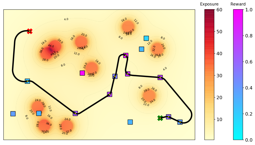
Figure 1: Minimal Exposure Dubins Orienteering Problem: given initial and final positions (red/green Xs), the goal is to compute a curvature-constrained path (black line) that visits the most rewarding locations (colored squares). The path is subjected to a limited travel budget and it must minimize the exposure to a known sensor field (reddish regions).

To solve this problem, we propose the use of an evolutionary algorithm that iteratively selects and evaluates distinct subsets of locations and in which order they should be visited; varies the orientations on each location; and attempts different feasible turning radii on the connecting segments, which aid to reduce the exposure. Results confirm that there is an inverse relationship between the collected reward and the path exposure. In other words, to avoid certain zones the agent will probably have to visit a smaller number of locations. However, by analyzing the behavior of the Pareto front we conclude that the approach can efficiently find a diverse set of solutions that simultaneously optimize both objectives.

II Related Work

A fundamental problem in Robotics is the generation of paths that are either length or time optimized, and a diverse collection of formulations and techniques to this challenge have been proposed in the literature.

The Orienteering Problem (OP) [2] is a multi-level optimization problem usually described as the combination of the Knapsack Problem (select subset of points) and the Traveling Salesman Problem (define the order of visit). The goal is to maximize the sum of the rewards associated with each location, however, considering a certain limited travel budget (e.g., length, time, energy, etc.). In most cases, this problem considers only a simple Euclidean metric to determine and represent the path, which may not be very representative.

In real-world scenarios, a large number of vehicles present motion constraints, and such characteristics must be taken into account when searching for solutions [6]. Recently, the Dubins Orienteering Problem (DOP) has been introduced [3], which considers the case of vehicles subjected to a bounded turning radius (Dubins vehicles [7]). Besides the selection of the subset of locations and sequence of visit, in this case, the orientation on each position must also be determined, which increases the complexity. The authors have employed the Variable Neighborhood Search (VNS) metaheuristic to solve this NP-hard problem.

Generally, routing problems such as the OP and DOP do not consider certain characteristics of the environment, and the determination of a safe path is also a fundamental requirement. Therefore, it is important to consider the presence of threatening zones, which can encompass from regular obstacles to regions that have a more continuous impact on the agent (e.g. detection probability).

The Minimal Exposure Path (MEP) [5] problem considers the case where an agent must minimize the exposure to certain regions in the environment. This concept introduced in [8] defines exposure as the capacity a sensor field possesses of perceiving a target along an arbitrary path. This problem is critical as it is usually associated with the coverage quality of a Wireless Sensor Network (WSN).

The first studies addressed the MEP problem with classic methods, such as grid-based approaches and Voronoi diagrams [9, 10]. Although simple to implement, such methods are not accurate enough, presenting difficulties in reaching the optimal solution [11]. They also have limitations dealing with heterogeneous networks or a large number of sensor nodes [12]. Due to the high complexity of the MEP, most of the recent literature has employed heuristics such as genetic algorithms [13, 14, 11]. Different approaches have also been applied for aerial robots with dynamic constraints to avoid threatening zones in 3D [15, 16].

To the best of our knowledge, this is the first work in which both DOP and MEP formulations are addressed simultaneously as a multi-objective problem, whose application can be extended to a broad range of more realistic contexts.

III Preliminaries

III-A Dubins curve

The Dubins model [7] considers vehicles that move in $\mathbb{R}^{2}$ along a path that respects a bounded curvature $\eta$, i.e.:

$$\dot{\vec{q}}=\begin{bmatrix}\dot{x}\\ \dot{y}\\ \dot{\theta}\end{bmatrix}=\mathit{v}\begin{bmatrix}\cos\theta\\ \sin\theta\\ u/\rho\end{bmatrix},$$

where $\mathit{v}\in\mathbb{R}^{+}$ is a constant linear speed and $u\in\{-1,\leavevmode\nobreak\ 0,\leavevmode\nobreak\ 1\}$. The curvature $\eta$ is inversely proportional to the minimum turning radius $\rho_{\textrm{min}}$ the vehicle is capable of executing.

This model is broadly adopted in robotics since it encompasses a large class of nonholonomic vehicles that range from Ackerman steering cars to fixed-wing aircrafts.

Definition 1.

A Dubins curve $\mathcal{D}_{\rho_{\textrm{min}}}(\vec{q}_{i},\vec{q}_{j})$ between two configurations $\vec{q}_{i}$ and $\vec{q}_{j}$ represents the shortest feasible path for a vehicle with minimum turning radius $\rho_{\textrm{min}}$ [7], and its length is given by $\mathit{d}_{\rho_{\textrm{min}}}:\text{SE}(2)\times\text{SE}(2)\rightarrow\mathbb{R}^{+}$.

III-B Sensing model

Threatening zones are modeled as a known deployed sensor field $\boldsymbol{\mathcal{N}}=\left\{\vec{n}_{1},\vec{n}_{2},\ldots,\vec{n}_{\mathit{n}}\right\}$, where $\vec{n}_{i}\in\mathbb{R}^{2}$ is the position of the $i$-th sensor node. Different sensing models can be found in the literature [12], from Boolean disks to probabilistic ones. We consider the broadly used attenuated disk coverage model since it accurately reflects the detection capability [14, 11].

Definition 2.

The sensing function $S(\cdot)$ provides the energy value of a target at a point $\vec{x}\in\mathbb{R}^{2}$ detected by a single sensor $\vec{n}_{i}$, given by

$$S(\vec{n}_{i},\vec{x})=\frac{\mathit{\alpha}}{\|\vec{n}_{i}-\vec{x}\|^{\mu}},$$ (1)

where $\mathit{\alpha}$ and $\mu$ are known positive constants related to the sensor and environment, while $\|\cdot\|$ is the Euclidean norm.

IV Problem Formulation

Let $\boldsymbol{\mathcal{P}}=\left\{\vec{p}_{1},\ldots,\vec{p}_{\mathit{m}}\right\}$ be a set of target locations, $\vec{p}_{i}\in\mathbb{R}^{2}$, each one with an associated reward $\mathit{r}(\vec{p}_{i})\in\mathbb{R}^{+}$. The OP aims to determine a subset $\boldsymbol{\mathcal{P}}_{k}\subseteq\boldsymbol{\mathcal{P}}$ and a sequence of visit that maximizes the accumulated reward, where the visiting path must respect a predefined travel budget $T_{\textrm{max}}$. It is assumed that the initial and final positions are fixed and given, and their rewards are $\mathit{r}(\vec{p}_{1})=\mathit{r}(\vec{p}_{m})=0$.

In the Dubins Orienteering Problem [3], the vehicle must assume a particular orientation at each location, and the determination of this configuration is also part of the problem. The final visiting path is a continuous map $\gamma:[0,1]\to\mathcal{L}$, $\gamma(0)=\vec{q}_{1}$ and $\gamma(1)=\vec{q}_{\mathit{m}}$, formed by Dubins curves:

$$\mathcal{L}=\bigcup_{i=1}^{k-1}\mathcal{D}_{\rho_{\textrm{min}}}(\vec{q}_{i},\vec{q}_{i+1}),$$ (2)

where $k$ defines subset $\boldsymbol{\mathcal{P}}_{k}$ of locations that will be visited. The orientation of two Dubins curves that meet at the same position must be equal, and $|\mathcal{L}|=\sum_{i=1}^{k-1}\mathit{d}_{\rho_{\textrm{min}}}(\vec{q}_{i},\vec{q}_{i+1})$ denotes the length of the path.

In this paper, the orienteering problem is addressed in the presence of a known deployed sensor field $\boldsymbol{\mathcal{N}}$. The concept of sensor field intensity is associated with the likelihood of a given target being detected at a location $\vec{x}$ by any of the sensors nodes [8]. Similar to the sensing function $S(\cdot)$, there are different forms of estimating the field intensity $I$, and we consider the all-sensor field intensity function, given by:

$$I(\boldsymbol{\mathcal{N}},\vec{x})=\sum_{i\in\boldsymbol{\mathcal{N}}}S(\vec{n}_{i},\vec{x}).$$ (3)

The field intensity function is used to calculate exposure $E$, which is related to the probability of a target being detected traveling at constant speed along an arbitrary path [10]. Given the Dubins path $\mathcal{L}$, it can be written as:

$$E(\boldsymbol{\mathcal{N}},\mathcal{L})=\int_{0}^{|\mathcal{L}|}I(\boldsymbol{\mathcal{N}},\mathcal{L}(s))ds.$$ (4)

Problem 1 (Minimal Exposure Dubins OP).

Given a set of target locations $\boldsymbol{\mathcal{P}}=\{\vec{p}_{i}\}_{i=1}^{\mathit{m}}$, each location $i$ with a known associated reward $\mathit{r}(\vec{p}_{i})$, and a sensor field formed by a set of nodes $\boldsymbol{\mathcal{N}}=\{\vec{n}_{i}\}_{i=1}^{\mathit{n}}$. Determine a path $\mathcal{L}$ that visits a subset of locations $\boldsymbol{\mathcal{P}}_{k}\subseteq\boldsymbol{\mathcal{P}}$ to maximize the total collected reward, whilst minimizes the exposure. Formally:

$$\max_{\leavevmode\nobreak\ \mathcal{L}} \displaystyle\sum_{\vec{p}\in\boldsymbol{\mathcal{P}}_{k}}\mathit{r}(\vec{p}),$$ (5)

$$\min_{\leavevmode\nobreak\ \mathcal{L}} E(\boldsymbol{\mathcal{N}},\mathcal{L}),$$ (6)

subject to $$\leavevmode\nobreak\ |\mathcal{L}|\leq T_{\textrm{max}}.$$ (7)

This problem (simplified as to define $\mathcal{L}$) involves the selection of the $k$ locations that will compose $\boldsymbol{\mathcal{P}}_{k}$ and their permutation, as well as the appropriate orientation at each location. Furthermore, we have to design the path in such a way that it avoids the threatening zones, in our case, by locally adjusting the turning radius.

V Methodology

The Minimal Exposure Dubins Orienteering Problem is constituted by both combinatorial and continuous optimization components. The combinatorial part of the problem is related to the subset selection of the most rewarding locations and the determination of the sequence of visits. The continuous part deals with the assignment of the vehicle’s orientation at the locations and the selection of a feasible and convenient turning radius, where both greatly affect the path shape.

Considering the high dimensionality of the search space, the problem is quite intractable, and finding efficient methods is an open challenge. In this context, evolutionary-based approaches proved to be a suitable option. Genetic Algorithm (GA) mimics evolutionary processes found in nature, working to find the fittest individual after a series of operations such as selection, reproduction, and mutation.

In multi-objective optimization problems, the usual concept of a single optimum solution (fittest individual) does not apply directly. Usually, the goal is to obtain different solutions with as many associated values as objectives. The best solutions for such problems belong to what is called a Pareto front, where all options are considered acceptable and equally good.

An important difference between multi-objective evolutionary algorithms over single-objective ones is in how to compare individuals, necessary in the selection phase. The selection is based on the dominance between individuals, given the objective dimensions. Usually, it is used a tournament selection considering a distance operator combined with a Pareto-based sorting (e.g., NSGA-II, SPEA2, etc.).

V-A Encoding

The chromosome is encoded as an array of tuples (Fig. 2), which represents a permutation of the locations to be visited as well as specific parameters to the calculation of the connecting Dubins curves. The indices of the genes correspond to the positions that must be visited.

$\langle\vec{p}_{\Sigma_{1}},\theta_{1},\rho_{1}\rangle$

$\langle\vec{p}_{\Sigma_{2}},\theta_{2},\rho_{2}\rangle$

$\ldots$

$\langle\vec{p}_{\Sigma_{\mathit{m}}},\theta_{\mathit{m}},\rho_{\mathit{m}}\rangle$

Figure 2: Chromosome structure.

The definition of $\boldsymbol{\mathcal{P}}_{k}$ and the permutation are based on a random-key scheme [17]. Each gene (tuple) in the chromosome has a parameter $\Sigma\in[0,1]$ that defines the order, and which is uniformly selected at random during initialization. A negative value will be used to represent that the location is not part of the solution, i.e., will not be visited. The start and goal locations receive $\Sigma_{1}=0$ and $\Sigma_{\mathit{m}}=1$.

The gene also has $\theta\in[0,2\pi)$ and $\rho\in[\rho_{\textrm{min}},\rho_{\textrm{max}}]$, which represent the orientation the vehicle must assume at a given location and the value of the turning radius used to determine the curve to the next location in the sequence, respectively.

V-B Fitness evaluation

Initially, we must decode the chromosome to obtain a solution (visit path). Hereupon, genes with $\Sigma=-1$ are discarded. We assume the remaining genes represent a valid solution, i.e., a path that respects $T_{\textrm{max}}$, as this validation is done during the generation of the offspring.

First, the genes are sorted by their random keys in ascending order. Next, we construct the path accordingly to Eq. (2). Each segment will be determined by considering the gene-specific values for the orientation and turning radius.

Finally, the fitness of the individual comprises the collected reward and the path’s exposure, determined by Eq. (4).

V-C Crossover

The crossover is responsible for the exploitation of the already known solutions, i.e., repeat decisions (in our case exchange individual genes) that have worked well so far.

This step will only exchange the values of the attributes, but not the index of the location a gene assigned to. This allows us to apply different types of operators and not only order-restricted ones. The well-known two-point crossover is a suitable and convenient option in our case, as it can produce changes considering only portions of the individual.

Then, we evaluate the validity of each new individual and adjust it if necessary. If the travel budget limit is violated, we repeatedly remove at random nodes that belong to the path, i.e., assign $\Sigma=-1$, until feasibility is achieved.

V-D Mutation

The mutation step brings innovation (exploration of the search space) and occurs internally to the individual.

In our context, it is responsible to randomly select new values to the order of visit, the orientation at a certain location, and the turning radius of the curve connecting two consecutive points in the sequence.

A different permutation is achieved by assigning a new value for $\Sigma$ in the $(0,1)$ interval. The start and goal locations do not suffer any change, and their values remain the same as they were initialized throughout the generations.

The heading $\theta$ will be updated accordingly to a von Mises (circular normal) distribution with mean $\mu$ and dispersion $\kappa$:

$$p(x)=\frac{e^{\kappa\cos(x-\mu)}}{2\pi I_{0}(\kappa)},$$ (8)

where $I_{0}(\kappa)$ is the modified Bessel function of order 0.

In our case, the mean $\mu$ will be defined as the current orientation. This distribution was chosen as it provides a good balance between the probability of searching in its vicinity and attempting a completely different new value.

Another innovative aspect of our approach is the variation of the turning radius along the path. New values will be uniformly chosen at random in an interval defined by the vehicle-specific constraint ($\rho_{\textrm{min}}$) and a scenario-related one ($\rho_{\textrm{max}}$). This is key to minimize the exposure of a path, however, the increase in the length can impact the collected reward (less visited locations) given the travel budget.

Finally, after the new values are assigned, the same budget violation check and correction operation mentioned in the previous step are executed to avoid invalid individuals.

VI Experiments

The simulation framework was implemented with Python 3.7 and uses the DEAP [18] library. The sensing function for all sensors considers coefficients $\mathit{\alpha}=50$ and $\mu=2$. We also apply a threshold where $S(\cdot)>30$.

VI-A Dataset

Since this is the first time the problem is being tackled, we propose two new test instances to the MEDOP and make them available.

• Scenario A: A 30m x 22m environment, with 11 nodes displaced in a cross shape. There are 18 locations to be visited, with rewards in $\{0.2,0.4,0.6,0.8,1.0\}$.

• Scenario B: A 30m x 30m environment, with 8 nodes displaced in a grid formation. There are 15 locations to be visited, with rewards in $\{0.2,0.4,0.6,0.8,1.0\}$.

VI-B Illustrative example

Initially, we present an illustrative example for better visualization of the test instances and understanding of the achieved results. In this example, we consider $T_{\textrm{max}}=100$ and $\rho\in[1.0,2.0]$ for both scenarios. Table I summarizes the parameters used for our evolutionary algorithm.

Table I: Algorithm parameters.

Parameter	Value
Population size	400
Number of generations	400
Selection method	NSGA-III (reference-point)
Crossover probability	0.8
Crossover operator	Two-point crossover
Mutation probability (individual)	0.4
Mutation probability (gene)	0.02
Dispersion (von Mises)	$\kappa=2.0$

Figures 3 and 4 show different solutions for the Scenario A and Scenario B instances, respectively. These solutions are in different parts of the final Pareto front, and it is possible to observe the trade-off between Reward and Exposure. Table II presents the extreme values of the frontier for each instance.

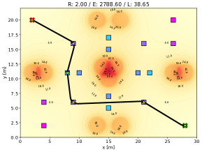
(a)

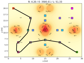
(b)

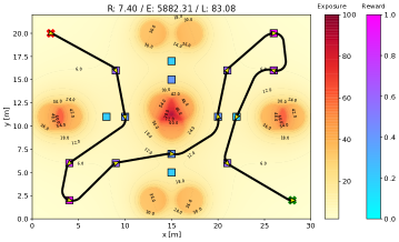
(c)

Figure 3: Example solutions along the Pareto front for Scenario A ($T_{\textrm{max}}=100$, $\rho\in[1.0,2.0]$). The title shows the values for Reward (R), Exposure (E), and Length (L) of the solutions.

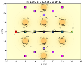
(a)

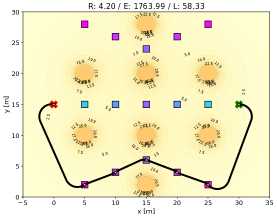
(b)

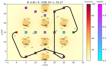
(c)

Figure 4: Example solutions along the Pareto front for Scenario B ($T_{\textrm{max}}=100$, $\rho\in[1.0,2.0]$). The title shows the values for Reward (R), Exposure (E), and Length (L) of the solutions.

Table II: Pareto front extreme solutions.

	Scenario A		Scenario B
	min	max	min	max
Reward	1.40	7.60	0.80	7.20
Exposure	2682.81	6671.75	1491.30	5440.37
Length	36.67	88.91	30.18	99.60

When tackling with multi-objective optimization problems, any of the Pareto front solutions are similarly good and acceptable. Therefore, a decision-making process can use different criteria to select the most adequate one, and the goal of a proper methodology for such problems is to provide it with a reasonable amount of rather distinct options.

For comparison purposes, we also solve the same instances considering only the reward objective ($\boldsymbol{\mathcal{N}}=\emptyset$). As can be seen in Fig. 5, by not taking into account the exposure restriction we can achieve a higher collected reward. Furthermore, the best individuals tend to keep $\rho$ close too $\rho_{\textrm{min}}$, as this helps to add more locations to the path.

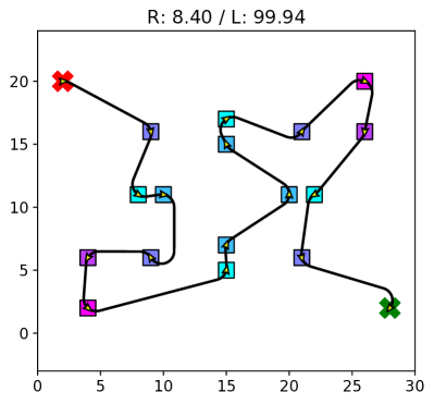
(a) MEDOP A

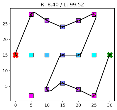
(b) MEDOP B

Figure 5: Single-objective solutions ($T_{\textrm{max}}=100$, $\rho\in[1.0,2.0]$).

A discussion about the use of the methodology for the single-objective case is presented in the next section.

VI-C Single-objective OP

Although our method is also applicable to the single-objective OP case, it was not designed for that purpose. Since we are tackling with multiple objectives, the final result is a set of optimal solutions. Hence, the goal is not only the convergence to an optimal solution but also the diversity of the solutions, which might assist a decision-making step.

Figure 6 presents a result of our method for the well-known Set 66 [19] dataset, considering $T_{\textrm{max}}=130$ and a fixed value of $\rho=0.7$. Figure 6a shows the result using the methodology as proposed (with $\kappa=8.0$). The genetic operators might be too simplistic for more dense and complex scenarios (orientations are challenging). Figure 6b shows the result considering a new operation during the mutation that simply tries to align the orientations of consecutive locations.

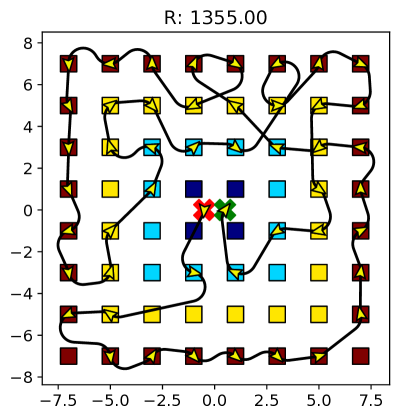
(a) Methodology

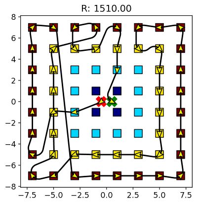
(b) Methodology+Alignment

Figure 6: Results for Set 66 [19] dataset ($T_{\textrm{max}}=130$, $\rho=0.7$).

Table III compares our results with other approaches in the literature. As can be seen, we achieve about $80\%-90\%$ of the state-of-the-art, however, with a simpler approach and without considering the assist of local search procedures.

Table III: Results for Set 66 dataset ($T_{\textrm{max}}=130$, $\rho=0.7$).

VNS [3]	Hybrid GA [4]	Ours	Ours (aligned)
1675	1670	1355	1510

Besides the satisfactory results when compared to other methods, in our case it is not recommended to explicitly benefit one objective over the other, for example, by applying the alignment strategy [20]. However, this shows the method is adaptable to easily incorporate more focused operators.

VI-D Numerical analysis

In this section, we investigate the effectiveness of our approach accordingly to a significant number of simulations. The behavior will be evaluated considering different combinations for the travel budget and turning radius interval.

The experiments were performed considering both test instances presented in Sec. VI-A. We vary the parameters accordingly to the following: $T_{\textrm{max}}=\{60,80,100,120\}$ and $\rho_{\textrm{max}}=\{1.0,2.0,3.0,4.0\}$, with a fixed $\rho_{\textrm{min}}=1.0$. For each case, the algorithm is executed 30 times, and we select the solution with the highest reward and smallest exposure. The overall performance is assessed through the final Pareto front.

Figure 7 shows the different results for a fixed $\rho_{\textrm{max}}=2.0$ and different values for $T_{\textrm{max}}$. As expected, a greater budget allows for the collection of more rewards. The behavior of all scenarios is similar, as there is not much room for different solutions with the fixed and equal turning radius interval.

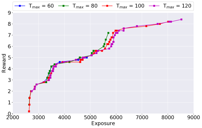
Figure 7: Test Instance - Scenario A. Final Pareto fronts for different values of $T_{\textrm{max}}$ and fixed $\rho_{\textrm{max}}=2.0$.

Figure 8 shows the results for a fixed $T_{\textrm{max}}=100$ and varying $\rho_{\textrm{max}}$. The following can be observed in this case: (i) it is possible to achieve a reduction on the exposure with greater values of $\rho_{\textrm{max}}$; (ii) to avoid certain regions and still respect the travel budget some locations will have to be removed from the path, resulting in a less collected reward. Hence, an intermediary value for $\rho_{\textrm{max}}$ seems the best choice.

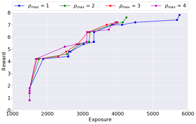
Figure 8: Test Instance - Scenario B. Final Pareto fronts for different values of $\rho_{\textrm{max}}$ and fixed $T_{\textrm{max}}=100$.

Due to space limitation, just partial results are presented here, the complete set of results can be found online.

VI-E Closed path

The OP was originally called Selective Traveling Salesman Problem [21], since it considered a circuit (i.e., $\vec{p}_{1}=\vec{p}_{\mathit{m}}$). Such formulation is a good representation of real-world scenarios, where vehicles usually leave and return to a common location (base). Considering this case, our problem can be seen as a variant of the Dubins Traveling Salesman Problem (DTSP) with budget and exposure constraints, and the methodology can be applied directly.

Figure 9 shows solutions of our approach for this case, with $T_{\textrm{max}}=120$ and different intervals for the turning radius. As can be seen, with the chance of varying the turning radius it is possible to modify the path and reduce the exposure, however, with an increase in the length. This corroborates with the previous sections, showing that focusing on achieving the shortest path is not the appropriate decision for the MEDOP.

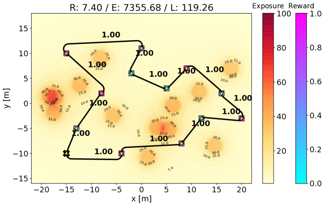
(a) $\rho_{\textrm{min}}=1.0,\rho_{\textrm{max}}=1.0$

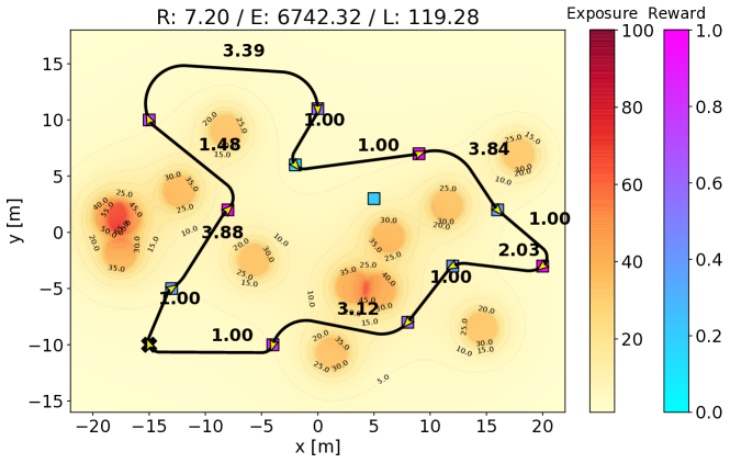
(b) $\rho_{\textrm{min}}=1.0,\rho_{\textrm{max}}=4.0$

Figure 9: Closed path examples ($T_{\textrm{max}}=120$). The bold numerals represent the turning radius used on that segment.

VII Conclusion and Future Work

In this paper, we introduced the Minimal Exposure Dubins Orienteering Problem (MEDOP), a multi-objective routing problem for bounded-curvature vehicles. The goal is to compute a path that maximizes the collected reward in predefined locations, while minimizes the exposure to threatening zones. This path is subjected to a limited travel budget, for example, time, length, or energy consumption.

The proposed methodology consists of an evolutionary algorithm that, in a combined manner, evaluates different sequences of visits, orientation on each location, and turning radius on each segment. Since our cost function is based on two objectives, we generate a set of fully viable solutions, and our evaluation is based on the Pareto front.

Results show that our approach can produce outcomes that have an adequate compromise between both objectives. Furthermore, it also contributes to the diversity of the solutions, which is a fundamental requirement in a decision-making step of multi-objective optimization problems.

Future research directions includes the use of multiple vehicles and more realistic environments filled with static or dynamic obstacles [22]. We also intend to address heterogeneous and dynamic sensor fields (e.g., moving nodes), and time-varying rewards on the locations.

References

- [1] D. G. Macharet and M. F. M. Campos, “A survey on routing problems and robotic systems,” Robotica, vol. 36, no. 12, p. 1781–1803, 2018.
- [2] I.-M. Chao, B. L. Golden, and E. A. Wasil, “A fast and effective heuristic for the orienteering problem,” European Journal of Operational Research, vol. 88, no. 3, pp. 475–489, 2 1996.
- [3] R. Pěnička, J. Faigl, P. Váňa, and M. Saska, “Dubins Orienteering Problem,” IEEE Robotics and Automation Letters, vol. 2, no. 2, pp. 1210–1217, 2017.
- [4] N. Tsiogkas and D. M. Lane, “DCOP: Dubins Correlated Orienteering Problem Optimizing Sensing Missions of a Nonholonomic Vehicle Under Budget Constraints,” IEEE Robotics and Automation Letters, vol. 3, no. 4, pp. 2926–2933, 10 2018.
- [5] G. Veltri, Q. Huang, G. Qu, and M. Potkonjak, “Minimal and Maximal Exposure Path Algorithms for Wireless Embedded Sensor Networks,” in 1st Int. Conf. on Embedded Networked Sensor Systems, ser. SenSys ’03. New York, NY, USA: Association for Computing Machinery, 2003, p. 40–50.
- [6] S. M. LaValle, Planning Algorithms. New York, NY, USA: Cambridge University Press, 2006.
- [7] L. E. Dubins, “On Curves of Minimal Length with a Constraint on Average Curvature, and with Prescribed Initial and Terminal Positions and Tangents,” American Journal of Mathematics, vol. 79, no. 3, pp. 497–516, 1957.
- [8] S. Meguerdichian, F. Koushanfar, G. Qu, and M. Potkonjak, “Exposure in Wireless Ad-Hoc Sensor Networks,” in 7th Annual Int. Conf. on Mobile Computing and Networking, ser. MobiCom ’01. New York, NY, USA: Association for Computing Machinery, 2001, p. 139–150.
- [9] V. Phipatanasuphorn and Parameswaran Ramanathan, “Vulnerability of sensor networks to unauthorized traversal and monitoring,” IEEE Trans. on Computers, vol. 53, no. 3, pp. 364–369, March 2004.
- [10] H. N. Djidjev, “Efficient computation of minimum exposure paths in a sensor network field,” in Distributed Computing in Sensor Systems, J. Aspnes, C. Scheideler, A. Arora, and S. Madden, Eds. Berlin, Heidelberg: Springer Berlin Heidelberg, 2007, pp. 295–308.
- [11] H. T. T. Binh, N. T. M. Binh, N. H. Ngoc, D. T. H. Ly, and N. D. Nghia, “Efficient approximation approaches to minimal exposure path problem in probabilistic coverage model for wireless sensor networks,” Applied Soft Computing, vol. 76, pp. 726–743, 2019.
- [12] M. Ye, Y. Wang, C. Dai, and X. Wang, “A Hybrid Genetic Algorithm for the Minimum Exposure Path Problem of Wireless Sensor Networks Based on a Numerical Functional Extreme Model,” IEEE Trans. on Vehicular Technology, vol. 65, no. 10, pp. 8644–8657, Oct 2016.
- [13] H. Feng, L. Luo, Y. Wang, M. Ye, and R. Dong, “A novel minimal exposure path problem in wireless sensor networks and its solution algorithm,” Int. Journal of Distributed Sensor Networks, vol. 12, no. 8, p. 1550147716664245, 2016.
- [14] T. M. B. Nguyen, C. M. Thang, D. N. Nguyen, and T. T. B. Huynh, “Genetic algorithm for solving minimal exposure path in mobile sensor networks,” in IEEE Symposium Series on Computational Intelligence (SSCI), Nov 2017, pp. 1–8.
- [15] B. Miller, K. Stepanyan, A. Miller, and M. Andreev, “3D path planning in a threat environment,” in 50th IEEE Conf. on Decision and Control and European Control Conf., 2011, pp. 6864–6869.
- [16] Y. Qu, Y. Zhang, and Y. Zhang, “Optimal flight path planning for UAVs in 3-D threat environment,” in Int. Conf. on Unmanned Aircraft Systems, ICUAS, 2014, pp. 149–155.
- [17] J. C. Bean, “Genetic Algorithms and Random Keys for Sequencing and Optimization,” ORSA Journal on Computing, vol. 6, no. 2, pp. 154–160, 1994.
- [18] F.-A. Fortin, F.-M. De Rainville, M.-A. Gardner, M. Parizeau, and C. Gagné, “DEAP: Evolutionary algorithms made easy,” Journal of Machine Learning Research, vol. 13, pp. 2171–2175, jul 2012.
- [19] I.-M. Chao, B. L. Golden, and E. A. Wasil, “A fast and effective heuristic for the orienteering problem,” European Journal of Operational Research, vol. 88, no. 3, pp. 475 – 489, 1996.
- [20] D. G. Macharet and M. F. M. Campos, “An Orientation Assignment Heuristic to the Dubins Traveling Salesman Problem,” in Advances in Artificial Intelligence – IBERAMIA 2014, A. L. Bazzan and K. Pichara, Eds. Cham: Springer International Publishing, 2014, pp. 457–468.
- [21] G. Laporte and S. Martello, “The selective travelling salesman problem,” Discrete Applied Mathematics, vol. 26, no. 2, pp. 193 – 207, 1990.
- [22] R. Pěnička, J. Faigl, and M. Saska, “Physical Orienteering Problem for Unmanned Aerial Vehicle Data Collection Planning in Environments With Obstacles,” IEEE Robotics and Automation Letters, vol. 4, no. 3, pp. 3005–3012, 2019.