Multi-spike solutions of a hybrid reaction-transport model

P. C. Bressloff,
Department of Mathematics, University of Utah
155 South 1400 East, Salt Lake City, UT 84112
Abstract

Numerical simulations of classical pattern forming reaction-diffusion systems indicate that they often operate in the strongly nonlinear regime, with the final steady-state consisting of a spatially repeating pattern of localized spikes. In activator-inhibitor systems such as the two-component Gierer-Meinhardt (GM) model, one can consider the singular limit DaDhmuch-less-thansubscript𝐷𝑎subscript𝐷D_{a}\ll D_{h}, where Dasubscript𝐷𝑎D_{a} and Dhsubscript𝐷D_{h} are the diffusivities of the activator and inhibitor, respectively. Asymptotic analysis can then be used to analyze the existence and linear stability of multi-spike solutions. In this paper, we analyze multi-spike solutions in a hybrid reaction-transport model, consisting of a slowly diffusing activator and an actively transported inhibitor that switches at a rate α𝛼\alpha between right-moving and left-moving velocity states. This class of model was recently introduced to account for the formation and homeostatic regulation of synaptic puncta during larval development in C. elegans. We exploit the fact that that the hybrid model can be mapped onto the classical GM model in the fast switching limit α𝛼\alpha\rightarrow\infty, which allows us to establish the existence of multi-spike solutions. Linearization about the multi-spike solution leads to a non-local eigenvalue problem that is used to derive stability conditions for the multi-spike solution for finite α𝛼\alpha.

1 Introduction

One major mechanism for self-organization between (and within cells) is the combination of diffusion and nonlinear chemical reactions. The notion that a reaction-diffusion (RD) system can spontaneously generate spatiotemporal patterns was first introduced by Turing in his seminal 1952 paper on morphogenesis [1]. He established the principle that two nonlinearly interacting chemical species differing significantly in their rates of diffusion can amplify spatially periodic fluctuations in their concentrations, resulting in the formation of a stable periodic pattern. The Turing mechanism for morphogenesis was subsequently refined by Gierer and Meinhardt [2], who showed that one way to generate a Turing instability is to have an antagonistic pair of molecular species known as an activator-inhibitor system, which consists of a slowly diffusing chemical activator and a quickly diffusing chemical inhibitor. For many years the only direct experimental evidence for spatiotemporal patterning of molecular concentrations came from the inorganic Belousov-Zhabotinsky reaction [3], until Kondo and Asai demonstrated the occurrence of the Turing mechanism in studies of animal coat patterning [4]. More recent advances in live cell imaging and gene knockout protocols are now allowing for a closer connection between theories of pattern formation and developmental cell biology. The range of models and applications of the Turing mechanism have expanded dramatically [5, 6, 7], including applications to ecology [8, 9] and systems neuroscience [10, 11]; in the latter case nonlocal synaptic interactions drive pattern forming instabilities rather than diffusion.

There are also a growing number of examples of spatiotemporal patterns of signaling molecules at the intracellular level [12, 13]. Such patterns typically regulate downstream structures such as the cytoskeleton and cell membrane, which then drive various mechanical processes including cell division and polarization [14, 15]. As highlighted by a number of authors [16, 17, 19, 20, 18], the classical activator-inhibitor mechanism for Turing pattern formation in cell development does not apply to many of the known examples of intracellular patterning during cell polarization and division. First, these latter processes are mass-conserving, at least on the time-scales for patterns to initially form and stabilize. Second, rather than two or more chemical species diffusing in the same medium and mutually affecting their rates of production and degradation, intracellular patterns typically involve the dynamical exchange of proteins between the cytoplasm and plasma membrane, resulting in associated changes of conformational state and a spatial redistribution of mass. One example of intracellular pattern formation without mass conservation is an RD model of the self-positioning of structural maintenance of chromosomes (SMC) protein complexes in E. coli, which are required for correct chromosome condensation, organization and segregation [22, 21, 23]. An interesting features shared by all of these model systems is that they tend to operate in the strongly non-linear regime (far from pattern onset). In the mass-conserving case, the final steady-state often consists of a single localized peak (spike) of the slowly diffusing activator, whereas multi-spike solutions can exist when mass is not conserved [23]. That is, the initial Turing pattern predicted from linear theory undergoes significant coarsening.

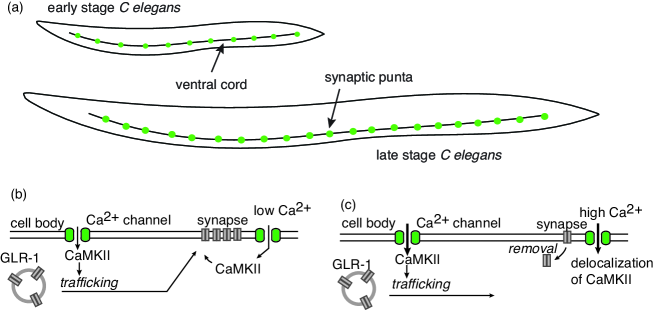
Based on experimental studies of synaptogenesis in Caenorhabditis elegans, we recently introduced a hybrid reaction-transport model for intracellular pattern formation, which involves the interaction between a passively diffusing component and an advecting component that switches between anterograde and retrograde motor-driven transport (bidirectional transport) [29, 30]. These components were identified as the protein kinase CaMKII and the glutamate receptor GLR-1, respectively. During larval development of C. elegans, the density of ventral and dorsal cord synapses containing the glutamate receptor GLR-1 is maintained despite significant changes in neurite length [24], see Fig. 1(a). It is known that the coupling of synapse number to neurite length requires CaMKII and voltage-gated calcium channels, and that CaMKII regulates the active (kinesin-based) transport and delivery of GLR-1 to synapses [25, 26, 27, 28], see Fig. 1(b). However, a long outstanding problem has been identifying a possible physical mechanism involving diffusing CaMKII molecules and motor-driven GLR-1 that leads to the homeostatic control of synaptic density. Using the classical Gierer and Meinhardt mechanism for reaction kinetics [2], we showed that our model supported Turing patterns on a one-dimensional domain of fixed length. (Turing pattern formation based on advecting species has also been considered within the context of chemotaxis [31].) Numerical simulations of the model using experimentally-based parameters generated patterns with a wavelength consistent with the synaptic spacing found in C. elegans, after identifying the in-phase CaMKII/GLR-1 concentration peaks as sites of new synapses. Extending the model to the case of a slowly growing 1D compartment, we subsequently showed how the synaptic density can be maintained during C. elegans growth, due to the insertion of new concentration peaks as the length of the compartment increases [30].

The above example of synaptogenesis in C. elegans motivates developing a more general theory of pattern formation in hybrid reaction-transport systems, particularly given the prevalence of both active and passive transport within cells. As part of such a program, we focus in this paper on multi-spike solutions far from pattern onset. Our previous work used linear stability analysis to identify regions in parameter space for a Turing instability close to pattern onset. However, numerical simulations indicated that the hybrid reaction-transport system operated in the strongly nonlinear regime, with the final steady-state consisting of a spatially repeating pattern of localized spikes. Although weakly nonlinear analysis is not applicable in the large amplitude regime, it is still possible to study the existence and stability of spike patterns in certain limits. For example, in the case of classical RD systems such as the Brusselator, Gierer-Meinhardt and Gray-Scott models, one can consider the singular limit DaDhmuch-less-thansubscript𝐷𝑎subscript𝐷D_{a}\ll D_{h}, where Dasubscript𝐷𝑎D_{a} and Dhsubscript𝐷D_{h} are the diffusivities of a slowly diffusing activator and a fast diffusing inhibitor, say. These systems support multi-spike solutions in which the activator is localized to narrow peak regions (spikes) within which the inhibitor is slowly varying. Asymptotic analysis can then be used to analyze the existence and linear stability of multi-spike solutions [32, 33, 34, 35, 36, 37], see also [23].
Refer to caption
Figure 1: (a) Schematic figure showing distribution of synaptic punta along ventral cord of early and late stage C. elegans. New synapses are inserted during development in order to maintain the synaptic density. (b) Regulation of transport and delivery of GLR-1 to synapses by CaMKII. Calcium influx through voltage-gated calcium channels activates CaMKII, which enhances the active transport and delivery of GLR-1 to synapses. Under conditions of increased excitation, higher calcium levels results in constitutively active CaMKII which fails to localize at synapses, leading to the removal of GLR-1 from synapses.

The structure of the paper is as follows. The hybrid reaction-transport model of [29, 30] is introduced in section 2, which is a three-component model consisting of a passively diffusing activator concentration P𝑃P and a pair of actively transported inhibitor concentrations A±subscript𝐴plus-or-minusA_{\pm}, which correspond to left-moving and right-moving velocity states, respectively. In steady-state, the full model is shown to be equivalent to the classical two-component GM model for (P,A)𝑃𝐴(P,A), where A=A++A𝐴subscript𝐴subscript𝐴A=A_{+}+A_{-}. In particular, the effective diffusivity of the inhibitor takes the form D=v2/(μ2+2α)𝐷superscript𝑣2subscript𝜇22𝛼D=v^{2}/(\mu_{2}+2\alpha), where v𝑣v is the speed of each velocity state, α𝛼\alpha is the switching rate, and μ2subscript𝜇2\mu_{2} is the degradation rate. In section 3 we construct a multi-spike solution of the steady-state model using the asymptotic method introduced in [32]. The one major difference is that in addition to the concentrations P,A𝑃𝐴P,A, one also has to determine the effective flux J=v(A+A)𝐽𝑣subscript𝐴subscript𝐴J=v(A_{+}-A_{-}). In section 4 we turn to the linear stability analysis of the multi-spike solution. This requires taking into account perturbations of all three components of the hybrid model, which ultimately leads to a non-local eigenvalue problem that is a generalization of the one obtained in [34]. Nevertheless, one can adapt the asymptotic analysis and winding number arguments of [34] to derive conditions for the stability of a multi-spike solution. In particular, we show how stability depends on the switching rate and degradation rate of the inhibitor.

2 Model

Consider a one-dimensional domain of fixed length 2L2𝐿2L. Let P(x,t)𝑃𝑥𝑡P(x,t) denote the concentration of a passively transported component at position x𝑥x at time t𝑡t and let A(x,t)𝐴𝑥𝑡A(x,t) denote the corresponding actively transported component. The latter is partitioned into two subpopulations: those that undergo anterograde transport (R+subscript𝑅R_{+}) and those that undergo retrograde transport (Rsubscript𝑅R_{-}) with A(x,t)=A+(x,t)+A(x,t)𝐴𝑥𝑡subscript𝐴𝑥𝑡subscript𝐴𝑥𝑡A(x,t)=A_{+}(x,t)+A_{-}(x,t). Individual particles randomly switch between the two advective states according to a two-state Markov process A+𝛼𝛼Asubscript𝐴𝛼𝛼subscript𝐴A_{+}\underset{\alpha}{\overset{\alpha}{\rightleftharpoons}}A_{-}, with transition rate α𝛼\alpha. Modeling the interactions between the active and passive using the classical activator-inhibitor system of Gierer and Meinhardt (GM) [2], we then have the following system of equations [29]:

Pt𝑃𝑡\displaystyle\frac{\partial P}{\partial t} =DP2Px2+f(P,A++A),absentsubscript𝐷𝑃superscript2𝑃superscript𝑥2𝑓𝑃subscript𝐴subscript𝐴\displaystyle=D_{P}\frac{\partial^{2}P}{\partial x^{2}}+f(P,A_{+}+A_{-}), (1a)
A+tsubscript𝐴𝑡\displaystyle\frac{\partial A_{+}}{\partial t} =vA+x+αAαA++g(P,A+),x[L,L],formulae-sequenceabsent𝑣subscript𝐴𝑥𝛼subscript𝐴𝛼subscript𝐴𝑔𝑃subscript𝐴𝑥𝐿𝐿\displaystyle=-v\frac{\partial A_{+}}{\partial x}+\alpha A_{-}-\alpha A_{+}+g(P,A_{+}),\quad x\in-[-L,L], (1b)
Atsubscript𝐴𝑡\displaystyle\frac{\partial A_{-}}{\partial t} =vAx+αA+αA+g(P,A),absent𝑣subscript𝐴𝑥𝛼subscript𝐴𝛼subscript𝐴𝑔𝑃subscript𝐴\displaystyle=v\frac{\partial A_{-}}{\partial x}+\alpha A_{+}-\alpha A_{-}+g(P,A_{-}), (1c)

where DPsubscript𝐷𝑃D_{P} is the diffusion coefficient of the passive component and v𝑣v is the speed of the motor-driven active component. The GM reaction terms are

f(P,A)=ρ1P2Aμ1P,g(P,A)=ρ2P2μ2A,formulae-sequence𝑓𝑃𝐴subscript𝜌1superscript𝑃2𝐴subscript𝜇1𝑃𝑔𝑃𝐴subscript𝜌2superscript𝑃2subscript𝜇2𝐴f(P,A)=\rho_{1}\frac{P^{2}}{A}-\mu_{1}P,\quad g(P,A)=\rho_{2}P^{2}-\mu_{2}A, (2)

so that P𝑃P is the activator and A±subscript𝐴plus-or-minusA_{\pm} the inhibitor. Here ρ1,ρ2subscript𝜌1subscript𝜌2\rho_{1},\rho_{2} represent the strength of interactions, and μ1,μ2subscript𝜇1subscript𝜇2\mu_{1},\mu_{2} are degradation rates. Equations (4) are supplemented by reflecting boundary conditions at the ends x=±L𝑥plus-or-minus𝐿x=\pm L:

C(x,t)x|x=±L=0,vR+(±L,t)=vR(±L,t).formulae-sequenceevaluated-at𝐶𝑥𝑡𝑥𝑥plus-or-minus𝐿0𝑣subscript𝑅plus-or-minus𝐿𝑡𝑣subscript𝑅plus-or-minus𝐿𝑡\displaystyle\left.\frac{\partial C(x,t)}{\partial x}\right|_{x=\pm L}=0,\quad vR_{+}(\pm L,t)=vR_{-}(\pm L,t). (3)

(Note that in the specific application to synaptogenesis in C. elegans, P𝑃P represented CaMKII and A±subscript𝐴plus-or-minusA_{\pm} represented GLR-1 [29, 30].)

Adding and subtracting the pair of equations (8b,c) and setting A=A++A𝐴subscript𝐴subscript𝐴A=A_{+}+A_{-} and J=vA+vA𝐽𝑣subscript𝐴𝑣subscript𝐴J=vA_{+}-vA_{-} yields the equivalent system

Pt𝑃𝑡\displaystyle\frac{\partial P}{\partial t} =DP2Px2+ρ1P2Aμ1P,absentsubscript𝐷𝑃superscript2𝑃superscript𝑥2subscript𝜌1superscript𝑃2𝐴subscript𝜇1𝑃\displaystyle=D_{P}\frac{\partial^{2}P}{\partial x^{2}}+\rho_{1}\frac{P^{2}}{A}-\mu_{1}P, (4a)
At𝐴𝑡\displaystyle\frac{\partial A}{\partial t} =Jx+2ρ2P2μ2A,x[L,L],formulae-sequenceabsent𝐽𝑥2subscript𝜌2superscript𝑃2subscript𝜇2𝐴𝑥𝐿𝐿\displaystyle=-\frac{\partial J}{\partial x}+2\rho_{2}P^{2}-\mu_{2}A,\quad x\in-[-L,L], (4b)
Jt𝐽𝑡\displaystyle\frac{\partial J}{\partial t} =v2Ax(2α+μ2)J.absentsuperscript𝑣2𝐴𝑥2𝛼subscript𝜇2𝐽\displaystyle=-{v^{2}}\frac{\partial A}{\partial x}-(2\alpha+\mu_{2})J. (4c)

Analogous to the reduction of a bidirectional transport model to the telegrapher’s equation [38], introducing the effective diffusivity

D=v22α+μ2,𝐷superscript𝑣22𝛼subscript𝜇2D=\frac{v^{2}}{2\alpha+\mu_{2}}, (5)

and taking the limit α𝛼\alpha\rightarrow\infty and v2superscript𝑣2v^{2}\rightarrow\infty with D𝐷D fixed (so that we can set HJ/t=0𝐻𝐽𝑡0\partial HJ/\partial t=0) yields the classical GM model for (P,A)𝑃𝐴(P,A) [2]

Pt𝑃𝑡\displaystyle\frac{\partial P}{\partial t} =DPd2Pdx2+ρ1P2Aμ1P,absentsubscript𝐷𝑃superscript𝑑2𝑃𝑑superscript𝑥2subscript𝜌1superscript𝑃2𝐴subscript𝜇1𝑃\displaystyle=D_{P}\frac{d^{2}P}{dx^{2}}+\frac{\rho_{1}P^{2}}{A}-\mu_{1}P, (6a)
At𝐴𝑡\displaystyle\frac{\partial A}{\partial t} =Dd2Adx2+2ρ2P2μ2A,D=v22α+μ2,formulae-sequenceabsent𝐷superscript𝑑2𝐴𝑑superscript𝑥22subscript𝜌2superscript𝑃2subscript𝜇2𝐴𝐷superscript𝑣22𝛼subscript𝜇2\displaystyle=D\frac{d^{2}A}{dx^{2}}+2\rho_{2}P^{2}-\mu_{2}A,\quad D=\frac{v^{2}}{2\alpha+\mu_{2}}, (6b)

In particular, we can identify D𝐷D as the diffusivity of the inhibitor in the reduced model. In addition, the time-independent versions of equations (4) and (6) are also equivalent for all finite values of α,D𝛼𝐷\alpha,D. It follows that the three-component hybrid reaction-transport model and the two-component RD model have the same steady-state solutions for (P,A)𝑃𝐴(P,A). This includes the unique uniform solution

P=ρ1μ22ρ2μ1,A±=ρ12μ24ρ2μ12,formulae-sequencesuperscript𝑃subscript𝜌1subscript𝜇22subscript𝜌2subscript𝜇1superscriptsubscript𝐴plus-or-minussuperscriptsubscript𝜌12subscript𝜇24subscript𝜌2superscriptsubscript𝜇12P^{*}=\frac{\rho_{1}\mu_{2}}{2\rho_{2}\mu_{1}},\quad A_{\pm}^{*}=\frac{\rho_{1}^{2}\mu_{2}}{4\rho_{2}\mu_{1}^{2}}, (7)

and multi-spike solutions. However, the corresponding eigenvalue problem obtained by linearizing about a given steady-state solution will differ in the two models, which means that their stability properties could also differ. A related issue is that, given a spatially varying steady-state solution for (P,A)𝑃𝐴(P,A) in the RD model, the corresponding hybrid system could support several different solutions for the flux J(x)𝐽𝑥J(x) and thus A±(x)subscript𝐴plus-or-minus𝑥A_{\pm}(x). In summary, one cannot simply carry over previous results for the existence and stability of spike solutions in the GM model of pattern formation [32].

One necessary condition for the occurrence of pattern formation in activator-inhibitor systems such as the GM model is that the inhibitor diffuses more quickly than the activator. Moreover, in order to obtain spike solutions of the form considered in Refs. [32, 33], the diffusivities should differ from each other by several orders of magnitude. The above analysis suggests that D𝐷D is the effective diffusivity of the actively transported component. We thus obtain the condition DPDmuch-less-thansubscript𝐷𝑃𝐷D_{P}\ll D. In the particular application to synaptogenesis in C. elegans the following order of magnitude parameter values were used [29, 30]: μ1,μ2,ρ11similar-tosubscript𝜇1subscript𝜇2subscript𝜌11\mu_{1},\mu_{2},\rho_{1}\sim 1/s, ρ21/(μM\rho_{2}\sim 1/(\mu M\cdots), α0.1similar-to𝛼0.1\alpha\sim 0.1/s, v1μsimilar-to𝑣1𝜇v\sim 1\mu\ m/s and DP0.01μsimilar-tosubscript𝐷𝑃0.01𝜇D_{P}\sim 0.01\ \mum2/s. In addition, the typical spacing of synaptic puncta is 3-4 per 10 μ𝜇\mum. It is clear that for this application, the effective diffusivity D1μ𝐷1𝜇D\approx 1\ \mum2/s, and thus the inequality DPDmuch-less-thansubscript𝐷𝑃𝐷D_{P}\ll D is satisfied. In this paper, we fix the units of time and space by setting μ1=1subscript𝜇11\mu_{1}=1 and L=1𝐿1L=1, and take ρ1=2ρ2=1subscript𝜌12subscript𝜌21\rho_{1}=2\rho_{2}=1. (In the case of C. elegans this corresponds to units t=1𝑡1t=1s and x=10μ𝑥10𝜇x=10\ \mum, assuming that L𝐿L is identified with a section of ventral cord containing approximately 3 or 4 synaptic puncta. An adult has a length of around 1 mm.) Writing DP=ϵ2subscript𝐷𝑃superscriptitalic-ϵ2D_{P}=\epsilon^{2} with 0<ϵ10italic-ϵmuch-less-than10<\epsilon\ll 1, we then have three remaining parameters μ2,α,Dsubscript𝜇2𝛼𝐷\mu_{2},\alpha,D. It is also more convenient to work with the variables P,A𝑃𝐴P,A and J𝐽J. Performing the rescaling PϵP/μ2𝑃italic-ϵ𝑃subscript𝜇2P\rightarrow{\epsilon}P/\mu_{2}, AϵA/μ2𝐴italic-ϵ𝐴subscript𝜇2A\rightarrow{\epsilon}A/\mu_{2}, JϵJ/μ22𝐽italic-ϵ𝐽superscriptsubscript𝜇22J\rightarrow\epsilon J/\mu_{2}^{2} and v2μ2v2superscript𝑣2subscript𝜇2superscript𝑣2v^{2}\rightarrow\mu_{2}v^{2} then gives

Pt𝑃𝑡\displaystyle\frac{\partial P}{\partial t} =ϵ22Px2+P2AP,absentsuperscriptitalic-ϵ2superscript2𝑃superscript𝑥2superscript𝑃2𝐴𝑃\displaystyle=\epsilon^{2}\frac{\partial^{2}P}{\partial x^{2}}+\frac{P^{2}}{A}-P, (8a)
1μ2At1subscript𝜇2𝐴𝑡\displaystyle\frac{1}{\mu_{2}}\frac{\partial A}{\partial t} =Jx+1ϵP2A,x[1,1],formulae-sequenceabsent𝐽𝑥1italic-ϵsuperscript𝑃2𝐴𝑥11\displaystyle=-\frac{\partial J}{\partial x}+\frac{1}{\epsilon}P^{2}-A,\quad x\in[-1,1], (8b)
12α+μ2Jt12𝛼subscript𝜇2𝐽𝑡\displaystyle\frac{1}{2\alpha+\mu_{2}}\frac{\partial J}{\partial t} =DAxJ.absent𝐷𝐴𝑥𝐽\displaystyle=-D\frac{\partial A}{\partial x}-J. (8c)

3 Existence of an N𝑁N-spike solution

We are interested in deriving conditions for the existence of multiple spike solutions in the limit ϵ0italic-ϵ0\epsilon\rightarrow 0. This type of solution consists of localized peaks in P𝑃P of width ϵitalic-ϵ\epsilon with P𝑃P exponentially small outside each spike, while A±subscript𝐴plus-or-minusA_{\pm} change slowly within each spike. Here we extend the asymptotic analysis of the classical GM model [32, 33]. Setting time-derivatives to zero in equations (8), we obtain the time-independent equations

00\displaystyle 0 =ϵ2d2Pdx2+P2AP,absentsuperscriptitalic-ϵ2superscript𝑑2𝑃𝑑superscript𝑥2superscript𝑃2𝐴𝑃\displaystyle=\epsilon^{2}\frac{d^{2}P}{dx^{2}}+\frac{P^{2}}{A}-P, (9a)
00\displaystyle 0 =DdAdxJ,absent𝐷𝑑𝐴𝑑𝑥𝐽\displaystyle=-D\frac{dA}{dx}-J, (9b)
00\displaystyle 0 =dJdx+1ϵP2A.absent𝑑𝐽𝑑𝑥1italic-ϵsuperscript𝑃2𝐴\displaystyle=-\frac{dJ}{dx}+\frac{1}{\epsilon}P^{2}-A. (9c)

Suppose that there are N𝑁N spikes at positions x1,,xNsubscript𝑥1subscript𝑥𝑁x_{1},\ldots,x_{N} with P𝑃P peaking at each point xjsubscript𝑥𝑗x_{j} such that

P(xj)=0,A(xj)=U,formulae-sequencesuperscript𝑃subscript𝑥𝑗0𝐴subscript𝑥𝑗𝑈P^{\prime}(x_{j})=0,\quad A(x_{j})=U, (10)

and U𝑈U independent of j𝑗j. (In order to apply asymptotic analysis, the spikes are located away from the boundaries x=0,1𝑥01x=0,1.)

Inside the inner region of the j𝑗j-th spike we introduce the stretched coordinate yj=ϵ1(xxj)subscript𝑦𝑗superscriptitalic-ϵ1𝑥subscript𝑥𝑗y_{j}=\epsilon^{-1}(x-x_{j}), and set P~(yj)=P(xj+ϵyj)~𝑃subscript𝑦𝑗𝑃subscript𝑥𝑗italic-ϵsubscript𝑦𝑗\widetilde{P}(y_{j})=P(x_{j}+\epsilon y_{j}), A~(yj)=A(xj+ϵyj)~𝐴subscript𝑦𝑗𝐴subscript𝑥𝑗italic-ϵsubscript𝑦𝑗\widetilde{A}(y_{j})=A(x_{j}+\epsilon y_{j}) and J~(yj)=J(xj+ϵyj)~𝐽subscript𝑦𝑗𝐽subscript𝑥𝑗italic-ϵsubscript𝑦𝑗\widetilde{J}(y_{j})=J(x_{j}+\epsilon y_{j}). Introduce the asymptotic expansions

P~=P~0+o(1),A~=A~0+ϵA~1+O(ϵ),J~=J~0+o(1),formulae-sequence~𝑃subscript~𝑃0𝑜1formulae-sequence~𝐴subscript~𝐴0italic-ϵsubscript~𝐴1𝑂italic-ϵ~𝐽subscript~𝐽0𝑜1\widetilde{P}=\widetilde{P}_{0}+o(1),\quad\widetilde{A}=\widetilde{A}_{0}+{\epsilon}\widetilde{A}_{1}+O(\epsilon),\quad\widetilde{J}=\widetilde{J}_{0}+o(1),

with

d2P~0dyj2+P~02A~0P~0=0,<yj<,formulae-sequencesuperscript𝑑2subscript~𝑃0𝑑superscriptsubscript𝑦𝑗2superscriptsubscript~𝑃02subscript~𝐴0subscript~𝑃00subscript𝑦𝑗\displaystyle\frac{d^{2}\widetilde{P}_{0}}{dy_{j}^{2}}+\frac{\widetilde{P}_{0}^{2}}{\widetilde{A}_{0}}-\widetilde{P}_{0}=0,\quad-\infty<y_{j}<\infty, (11)
dA~0dyj=0,DdA~1dyjJ~0=0,dJ~0dyj+P~02=0,formulae-sequence𝑑subscript~𝐴0𝑑subscript𝑦𝑗0formulae-sequence𝐷𝑑subscript~𝐴1𝑑subscript𝑦𝑗subscript~𝐽00𝑑subscript~𝐽0𝑑subscript𝑦𝑗superscriptsubscript~𝑃020\displaystyle\frac{d\widetilde{A}_{0}}{dy_{j}}=0,\quad-D\frac{d\widetilde{A}_{1}}{dy_{j}}-\widetilde{J}_{0}=0,\quad-\frac{d\widetilde{J}_{0}}{dy_{j}}+\widetilde{P}_{0}^{2}=0, (12)

and

P~0(0)=0,A~0(0)=U,A~1(0)=0.formulae-sequencesuperscriptsubscript~𝑃000formulae-sequencesubscript~𝐴00𝑈subscript~𝐴100\widetilde{P}_{0}^{\prime}(0)=0,\ \widetilde{A}_{0}(0)=U,\quad\widetilde{A}_{1}(0)=0. (13)

We also require P~00subscript~𝑃00\widetilde{P}_{0}\rightarrow 0 as |yj|subscript𝑦𝑗|y_{j}|\rightarrow\infty. The analysis of P~0subscript~𝑃0\widetilde{P}_{0}, A0~~subscript𝐴0\widetilde{A_{0}} and A1~~subscript𝐴1\widetilde{A_{1}} now proceeds in an identical fashion to the classical GM model [32]. (However, we also have the additional variable J𝐽J,which we will return to below). The first equation of (12) immediately implies that A~0(yj)=Usubscript~𝐴0subscript𝑦𝑗𝑈\widetilde{A}_{0}(y_{j})=U for all <yj<subscript𝑦𝑗-\infty<y_{j}<\infty. In addition, using phase plane analysis it can be shown that equation (11) has the solution [32]

P~0(yj)=32Usech2(yj/2):=Up(yj).subscript~𝑃0subscript𝑦𝑗32𝑈superscriptsech2subscript𝑦𝑗2assign𝑈𝑝subscript𝑦𝑗\widetilde{P}_{0}(y_{j})=\frac{3}{2}U\mbox{sech}^{2}\left(y_{j}/2\right):=Up(y_{j}). (14)

Therefore, integrating the equation for J~0subscript~𝐽0\widetilde{J}_{0} yields

[limyjJ~0limyjJ~0]=ΓU2,Γ=p~(y)2𝑑y=6.formulae-sequencedelimited-[]subscriptsubscript𝑦𝑗subscript~𝐽0subscriptsubscript𝑦𝑗subscript~𝐽0Γsuperscript𝑈2Γsuperscriptsubscript~𝑝superscript𝑦2differential-d𝑦6\left[\lim_{y_{j}\rightarrow\infty}\widetilde{J}_{0}-\lim_{y_{j}\rightarrow-\infty}\widetilde{J}_{0}\right]=\Gamma U^{2},\quad\Gamma=\int_{-\infty}^{\infty}\widetilde{p}(y)^{2}dy=6. (15)

Finally, substituting for J~0subscript~𝐽0\widetilde{J}_{0} using the second equation in (12) implies that

[limyjA~1limyjA~1]=ΓU2D.delimited-[]subscriptsubscript𝑦𝑗superscriptsubscript~𝐴1subscriptsubscript𝑦𝑗superscriptsubscript~𝐴1Γsuperscript𝑈2𝐷\left[\lim_{y_{j}\rightarrow\infty}\widetilde{A}_{1}^{\prime}-\lim_{y_{j}\rightarrow-\infty}\widetilde{A}_{1}^{\prime}\right]=-\frac{\Gamma U^{2}}{D}. (16)
Refer to caption
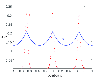
Figure 2: 3-spike solution obtained from asymptotic analysis with ϵ=0.02italic-ϵ0.02\epsilon=0.02, D=0.1𝐷0.1D=0.1, ρ1=μ1=2ρ2=μ=1subscript𝜌1subscript𝜇12subscript𝜌2𝜇1\rho_{1}=\mu_{1}=2\rho_{2}=\mu=1. Plots of A(x)𝐴𝑥A(x) and P(x)𝑃𝑥P(x).

Equation (16) acts as a jump condition for the first derivative of the solution for A𝐴A in the outer region. Since P0similar-to𝑃0P\sim 0 in the outer region, we can write A(x)=A0(x)+O(ϵ)𝐴𝑥subscript𝐴0𝑥𝑂italic-ϵA(x)=A_{0}(x)+O(\epsilon) with

Dd2A0dx2A0=0,x[1,1]\{x1,x2,,xN},formulae-sequence𝐷superscript𝑑2subscript𝐴0𝑑superscript𝑥2subscript𝐴00𝑥\11subscript𝑥1subscript𝑥2subscript𝑥𝑁D\frac{d^{2}A_{0}}{dx^{2}}-A_{0}=0,\quad x\in[-1,1]\backslash\{x_{1},x_{2},\ldots,x_{N}\}, (17)

and A0subscript𝐴0A_{0} continuous across xjsubscript𝑥𝑗x_{j} but A0superscriptsubscript𝐴0A_{0}^{\prime} discontinuous according to equation (16). That is,

Dd2A0dx2A0=ΓU2k=1Nδ(xxk),x[1,1],formulae-sequence𝐷superscript𝑑2subscript𝐴0𝑑superscript𝑥2subscript𝐴0Γsuperscript𝑈2superscriptsubscript𝑘1𝑁𝛿𝑥subscript𝑥𝑘𝑥11D\frac{d^{2}A_{0}}{dx^{2}}-A_{0}=-\Gamma U^{2}\sum_{k=1}^{N}\delta(x-x_{k}),\quad x\in[-1,1], (18)

with A0(x)=0superscriptsubscript𝐴0𝑥0A_{0}^{\prime}(x)=0 at x=0,1𝑥01x=0,1. Introducing the Neumann Green’s function

Dd2G(x;xk)dx2G(x;xk)𝐷superscript𝑑2𝐺𝑥subscript𝑥𝑘𝑑superscript𝑥2𝐺𝑥subscript𝑥𝑘\displaystyle D\frac{d^{2}G(x;x_{k})}{dx^{2}}-G(x;x_{k}) =δ(xxk),xG(0;xk)=0=xG(1;xk),formulae-sequenceabsent𝛿𝑥subscript𝑥𝑘subscript𝑥𝐺0subscript𝑥𝑘0subscript𝑥𝐺1subscript𝑥𝑘\displaystyle=-\delta(x-x_{k}),\ \partial_{x}G(0;x_{k})=0=\partial_{x}G(1;x_{k}), (19)
01G(x;xk)𝑑xsuperscriptsubscript01𝐺𝑥subscript𝑥𝑘differential-d𝑥\displaystyle\int_{0}^{1}G(x;x_{k})dx =1,absent1\displaystyle=1,

we can write the outer solution as

A0(x)=ΓU2j=1NG(x;xj).subscript𝐴0𝑥Γsuperscript𝑈2superscriptsubscript𝑗1𝑁𝐺𝑥subscript𝑥𝑗A_{0}(x)=\Gamma U^{2}\sum_{j=1}^{N}G(x;x_{j}). (20)

The explicit form of the 1D Green’s function is [32]

G(x;xk)={𝒜kcoshκ(1+x)/coshκ(1+xk)1<x<xk𝒜kcoshκ(1x)/coshκ(1xk)xk<x<1,𝐺𝑥subscript𝑥𝑘casessubscript𝒜𝑘𝜅1𝑥𝜅1subscript𝑥𝑘1𝑥subscript𝑥𝑘subscript𝒜𝑘𝜅1𝑥𝜅1subscript𝑥𝑘subscript𝑥𝑘𝑥1G(x;x_{k})=\left\{\begin{array}[]{cc}{\mathcal{A}}_{k}\cosh\kappa(1+x)/\cosh\kappa(1+x_{k})&\ -1<x<x_{k}\\ {\mathcal{A}}_{k}\cosh\kappa(1-x)/\cosh\kappa(1-x_{k})&\ x_{k}<x<1\end{array}\right., (21)

where

𝒜k=κ(tanhκ(1xk)+tanhκ(1+xk))1,κ=1/D.formulae-sequencesubscript𝒜𝑘𝜅superscript𝜅1subscript𝑥𝑘𝜅1subscript𝑥𝑘1𝜅1𝐷{\mathcal{A}}_{k}=\kappa\left(\tanh\kappa(1-x_{k})+\tanh\kappa(1+x_{k})\right)^{-1},\quad\kappa=\sqrt{1/D}. (22)

In particular,

j=1NG(x;xj)=12Dtanh(1/ND).superscriptsubscript𝑗1𝑁𝐺𝑥subscript𝑥𝑗12𝐷1𝑁𝐷\sum_{j=1}^{N}G(x;x_{j})=\frac{1}{2\sqrt{D}\tanh(1/N\sqrt{D})}. (23)

It remains to determine the constant U𝑈U. Setting x=xi𝑥subscript𝑥𝑖x=x_{i} in equation (20) yields the self-consistency condition

U=ΓU2j=1NG(xi;xj).𝑈Γsuperscript𝑈2superscriptsubscript𝑗1𝑁𝐺subscript𝑥𝑖subscript𝑥𝑗U=\Gamma U^{2}\sum_{j=1}^{N}G(x_{i};x_{j}). (24)

It follows that a symmetric N𝑁N spike solution will exist provided that the positions x1,,xNsubscript𝑥1subscript𝑥𝑁x_{1},\ldots,x_{N} are chosen such that the sum 𝒢=j=0N1G(xi;xj)𝒢superscriptsubscript𝑗0𝑁1𝐺subscript𝑥𝑖subscript𝑥𝑗{\mathcal{G}}=\sum_{j=0}^{N-1}G(x_{i};x_{j}) is independent of i𝑖i. It can be shown that this occurs for the equally spaced solution [32]

xj=1+2j1N,j=1,,N.formulae-sequencesubscript𝑥𝑗12𝑗1𝑁𝑗1𝑁x_{j}=-1+\frac{2j-1}{N},\quad j=1,\ldots,N. (25)

The non-trivial solution for the amplitude U𝑈U is then

U=1Γj=1NG(xi;xj).𝑈1Γsuperscriptsubscript𝑗1𝑁𝐺subscript𝑥𝑖subscript𝑥𝑗U=\frac{1}{\Gamma\sum_{j=1}^{N}G(x_{i};x_{j})}. (26)
Refer to caption
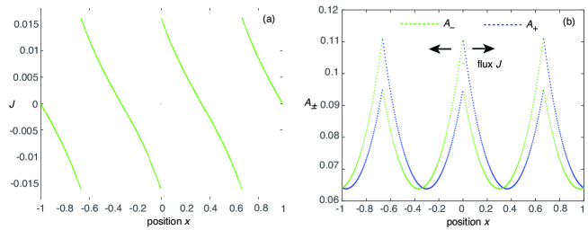
Figure 3: 3-spike solution obtained from asymptotic analysis with ϵ=0.02italic-ϵ0.02\epsilon=0.02, D=0.1𝐷0.1D=0.1, ρ1=μ1=2ρ2=μ=1subscript𝜌1subscript𝜇12subscript𝜌2𝜇1\rho_{1}=\mu_{1}=2\rho_{2}=\mu=1. (a) Plot of flux J(x)𝐽𝑥J(x). (c) Plots of A±(x)subscript𝐴plus-or-minus𝑥A_{\pm}(x).

So far everything has proceeded along the same lines as the analysis of spike solutions of the classical GM model. However, we also have the additional outer equation for J(x)=J0(x)+O(ϵ)𝐽𝑥subscript𝐽0𝑥𝑂italic-ϵJ(x)=J_{0}(x)+O(\epsilon):

J0(x)=DdA0dxx[1,1]\{x1,x2,,xN},formulae-sequencesubscript𝐽0𝑥𝐷𝑑subscript𝐴0𝑑𝑥𝑥\11subscript𝑥1subscript𝑥2subscript𝑥𝑁J_{0}(x)=-D\frac{dA_{0}}{dx}\quad x\in[-1,1]\backslash\{x_{1},x_{2},\ldots,x_{N}\}, (27)

with A0(x)subscript𝐴0𝑥A_{0}(x) given by equation (20) and J0subscript𝐽0J_{0} automatically satisfying the jump condition (15). Substituting for A0(x)subscript𝐴0𝑥A_{0}(x) gives

J0(x)=DΓU2k=1NxG(x;xk),x[1,1].formulae-sequencesubscript𝐽0𝑥𝐷Γsuperscript𝑈2superscriptsubscript𝑘1𝑁subscript𝑥𝐺𝑥subscript𝑥𝑘𝑥11J_{0}(x)=-D\Gamma U^{2}\sum_{k=1}^{N}\partial_{x}G(x;x_{k}),\quad x\in[-1,1]. (28)

In conclusion, in the limit ϵ0italic-ϵ0\epsilon\rightarrow 0 the leading order asymptotic solutions for the unscaled concentrations P𝑃P, A𝐴A and J𝐽J are of the form

P(x)Up([xxj]/ϵ),A(x)ΓU2j=1NG(x;xj),J(x)DΓU2k=1NxG(x;xk).formulae-sequencesimilar-to𝑃𝑥𝑈𝑝delimited-[]𝑥subscript𝑥𝑗italic-ϵformulae-sequencesimilar-to𝐴𝑥Γsuperscript𝑈2superscriptsubscript𝑗1𝑁𝐺𝑥subscript𝑥𝑗similar-to𝐽𝑥𝐷Γsuperscript𝑈2superscriptsubscript𝑘1𝑁subscript𝑥𝐺𝑥subscript𝑥𝑘P(x)\sim Up([x-x_{j}]/\epsilon),\quad A(x)\sim\Gamma U^{2}\sum_{j=1}^{N}G(x;x_{j}),\quad J(x)\sim-D\Gamma U^{2}\sum_{k=1}^{N}\partial_{x}G(x;x_{k}). (29)

In Figs. 2 and 3 we show an example of a 3-spike solution for ϵ=0.02italic-ϵ0.02\epsilon=0.02 and D=0.1𝐷0.1D=0.1. In particular, we see that the flux J𝐽J of the active component flows away from each peak such that the outer solutions for A+(x)subscript𝐴𝑥A_{+}(x) and A(x)subscript𝐴𝑥A_{-}(x) are asymmetric.

4 Linear stability analysis

In order to investigate the stability of an equilibrium spike solution, we introduce the perturbations

P(x,t)=P(x)+eλtΦ(x),A(x,t)=A(x)+eλtΨ(x),J(x,t)=J(x)+eλtΛ(x).formulae-sequence𝑃𝑥𝑡𝑃𝑥superscripte𝜆𝑡Φ𝑥formulae-sequence𝐴𝑥𝑡𝐴𝑥superscripte𝜆𝑡Ψ𝑥𝐽𝑥𝑡𝐽𝑥superscripte𝜆𝑡Λ𝑥P(x,t)=P(x)+{\mathrm{e}}^{\lambda t}\Phi(x),\quad A(x,t)=A(x)+{\mathrm{e}}^{\lambda t}\Psi(x),\quad J(x,t)=J(x)+{\mathrm{e}}^{\lambda t}\Lambda(x). (30)

Substituting into equations (8) and linearizing gives

(1+λ)Φ(x)1𝜆Φ𝑥\displaystyle(1+\lambda)\Phi(x) =ϵ2d2Φ(x)dx2+2P(x)A(x)Φ(x)P2(x)A2(x)Ψ(x),absentsuperscriptitalic-ϵ2superscript𝑑2Φ𝑥𝑑superscript𝑥22𝑃𝑥𝐴𝑥Φ𝑥superscript𝑃2𝑥superscript𝐴2𝑥Ψ𝑥\displaystyle=\epsilon^{2}\frac{d^{2}\Phi(x)}{dx^{2}}+2\frac{P(x)}{A(x)}\Phi(x)-\frac{P^{2}(x)}{A^{2}(x)}\Psi(x), (31a)
(1+τλ)Ψ(x)1𝜏𝜆Ψ𝑥\displaystyle(1+\tau\lambda)\Psi(x) =dΛ(x)dx+2P(x)ϵΦ(x),x[1,1],formulae-sequenceabsent𝑑Λ𝑥𝑑𝑥2𝑃𝑥italic-ϵΦ𝑥𝑥11\displaystyle=-\frac{d\Lambda(x)}{dx}+\frac{2P(x)}{\epsilon}\Phi(x),\quad x\in[-1,1], (31b)
(1+τ^λ)Λ(x)1^𝜏𝜆Λ𝑥\displaystyle(1+\widehat{\tau}\lambda)\Lambda(x) =DdΨ(x)dx.absent𝐷𝑑Ψ𝑥𝑑𝑥\displaystyle=-D\frac{d\Psi(x)}{dx}. (31c)

with

τ=1μ2,τ^=12α+μ2,D=v2τ^.formulae-sequence𝜏1subscript𝜇2formulae-sequence^𝜏12𝛼subscript𝜇2𝐷superscript𝑣2^𝜏\tau=\frac{1}{\mu_{2}},\quad\widehat{\tau}=\frac{1}{2\alpha+\mu_{2}},\quad D=v^{2}\widehat{\tau}. (32)

These equations are supplemented by the no-flux boundary conditions

Φ(±1)=Ψ(±1)=Λ(±1)=0.superscriptΦplus-or-minus1superscriptΨplus-or-minus1superscriptΛplus-or-minus10\Phi^{\prime}(\pm 1)=\Psi^{\prime}(\pm 1)=\Lambda^{\prime}(\pm 1)=0. (33)

Equation (32) implies that 0τ^τ0^𝜏𝜏0\leq\widehat{\tau}\leq\tau, and varying τ^^𝜏\widehat{\tau} from zero to τ𝜏\tau is equivalent to going from the fast switching regime α𝛼\alpha\rightarrow\infty to the slow switching regime α0𝛼0\alpha\rightarrow 0. In the following we investigate how the stability of the multi-spike solution depends on α𝛼\alpha.

Let us first consider the diffusion limit α,vformulae-sequence𝛼𝑣\alpha\rightarrow\infty,v\rightarrow\infty such that D𝐷D is fixed. Eliminating Λ(x)Λ𝑥\Lambda(x) gives

(1+λ)Φ(x)1𝜆Φ𝑥\displaystyle(1+\lambda)\Phi(x) =ϵ2d2Φ(x)dx2+2P(x)A(x)Φ(x)P2(x)A2(x)Ψ(x),absentsuperscriptitalic-ϵ2superscript𝑑2Φ𝑥𝑑superscript𝑥22𝑃𝑥𝐴𝑥Φ𝑥superscript𝑃2𝑥superscript𝐴2𝑥Ψ𝑥\displaystyle=\epsilon^{2}\frac{d^{2}\Phi(x)}{dx^{2}}+2\frac{P(x)}{A(x)}\Phi(x)-\frac{P^{2}(x)}{A^{2}(x)}\Psi(x), (34a)
(1+τλ)Ψ(x)1𝜏𝜆Ψ𝑥\displaystyle(1+\tau\lambda)\Psi(x) =Dd2Ψ(x)dx2+2P(x)ϵΦ(x),x[1,1].formulae-sequenceabsent𝐷superscript𝑑2Ψ𝑥𝑑superscript𝑥22𝑃𝑥italic-ϵΦ𝑥𝑥11\displaystyle=D\frac{d^{2}\Psi(x)}{dx^{2}}+\frac{2P(x)}{\epsilon}\Phi(x),\quad x\in[-1,1]. (34b)

This is identical to the eigenvalue problem for the classical GM model studied in [32, 34]. One finds that there are two sets of eigenvalues: large or O(1)𝑂1O(1) eigenvalues that are bounded away from zero as ϵ0italic-ϵ0\epsilon\rightarrow 0; small eigenvalues that approach zero as O(ϵ2)𝑂superscriptitalic-ϵ2O(\epsilon^{2}). The source of theses eigenvalues can be understood by considering the so-called shadow GM system in the limit D𝐷D\rightarrow\infty with τ=0𝜏0\tau=0. The linear operator of the latter has N𝑁N exponentially small eigenvalues that reflect the near translation invariance of the system and the existence of exponentially weak interactions between neighboring spikes and between spikes and the boundary. These become the small eigenvalues for finite D𝐷D is finite. The linear operator of the shadow system also has exactly one positive eigenvalue in the vicinity of each spike, which implies that an N𝑁N-spike solution is unstable on an O(1)𝑂1O(1) time-scale. However, as D𝐷D is decreased from infinity, the O(1)𝑂1O(1) eigenvalue near each spike moves into the left-half plane thus stabilizing the solution in the long-time limit. For D<𝐷D<\infty. N2𝑁2N\geq 2, and τ0𝜏0\tau\geq 0, the following results hold (see propositions 4 and 11 of [32] and proposition 5.3 of [34]).

Small eigenvalues. Consider a symmetric N𝑁N-spike solution and the associated linear operator (34) with τ=0𝜏0\tau=0. The O(ϵ2)𝑂superscriptitalic-ϵ2O(\epsilon^{2}) eigenvalues are negative only when D<DN𝐷superscriptsubscript𝐷𝑁D<D_{N}^{*}, where

DN=1[Nln(1+2)]2.superscriptsubscript𝐷𝑁1superscriptdelimited-[]𝑁122D_{N}^{*}=\frac{1}{[N\ln(1+\sqrt{2})]^{2}}. (35)

There are N1𝑁1N-1 small positive eigenvalues when D>DN𝐷superscriptsubscript𝐷𝑁D>D_{N}^{*} and λ=0𝜆0\lambda=0 is an eigenvalue of algebraic multiplicity N1𝑁1N-1 when D=DN𝐷superscriptsubscript𝐷𝑁D=D_{N}^{*}. Moreover, DNsuperscriptsubscript𝐷𝑁D_{N}^{*} is a decreasing function of N𝑁N, with D20.32superscriptsubscript𝐷20.32D_{2}^{*}\approx 0.32, D30.14superscriptsubscript𝐷30.14D_{3}^{*}\approx 0.14 and D40.08superscriptsubscript𝐷40.08D_{4}^{*}\approx 0.08, for example. These results persist to leading order when τ=O(1)𝜏𝑂1\tau=O(1).

Large eigenvalues. Let λ0subscript𝜆0\lambda_{0} be the O(1)𝑂1O(1) eigenvalue with the largest real part for τ=0𝜏0\tau=0. Then Re(λ0)<0Resubscript𝜆00\mbox{Re}(\lambda_{0})<0 when

D<DN1ΘN2,ΘN=N2ln[2+cos(π/N)+(2+cos(π/N))21)].D<D_{N}\equiv\frac{1}{\Theta_{N}^{2}},\quad\Theta_{N}=\frac{N}{2}\ln\left[2+\cos(\pi/N)+\sqrt{\left(2+\cos(\pi/N))^{2}-1\right)}\right]. (36)

On the other hand, Re(λ0)>0Resubscript𝜆00\mbox{Re}(\lambda_{0})>0 when D>DN𝐷subscript𝐷𝑁D>D_{N}. Note that DN>DNsubscript𝐷𝑁superscriptsubscript𝐷𝑁D_{N}>D_{N}^{*} and DNsubscript𝐷𝑁D_{N} is also a decreasing function of N𝑁N with D1=subscript𝐷1D_{1}=\infty, D20.58subscript𝐷20.58D_{2}\approx 0.58, D30.18subscript𝐷30.18D_{3}\approx 0.18 and D40.09subscript𝐷40.09D_{4}\approx 0.09, for example. It follows that there exists a parameter regime DN<D<DNsuperscriptsubscript𝐷𝑁𝐷subscript𝐷𝑁D_{N}^{*}<D<D_{N} where an N𝑁N-spike solution is stable on an O(1)𝑂1O(1) time-scale but unstable in the long-time limit. Finally, if τ=O(1)𝜏𝑂1\tau=O(1) then an N𝑁N-spike solution is unstable for any τ0𝜏0\tau\geq 0 when D>DN𝐷subscript𝐷𝑁D>D_{N}. For D>DN𝐷subscript𝐷𝑁D>D_{N} and τ0𝜏0\tau\geq 0, there are eigenvalues that are real and positive, and the resulting instability involves spikes being annihilated in finite time. On the other hand, for 0<D<DN0𝐷subscript𝐷𝑁0<D<D_{N}, an N𝑁N-spike solution is stable with respect to the O(1)𝑂1O(1) eigenvalues provided that 0ττN(D)0𝜏subscript𝜏𝑁𝐷0\leq\tau\leq\tau_{N}(D) for some critical time constant τNsubscript𝜏𝑁\tau_{N} (which can be determined numerically). When τ𝜏\tau crosses the critical value τN(D)subscript𝜏𝑁𝐷\tau_{N}(D), a synchronous oscillatory instability of the spike amplitudes is induced.

4.1 Derivation of nonlocal eigenvalue problem

Now suppose that v𝑣v and α𝛼\alpha are both finite. Since the left-hand sides of equations (31b,c) involve the factors (1+τλ)1𝜏𝜆(1+\tau\lambda) and (1+τ^λ)1^𝜏𝜆(1+\widehat{\tau}\lambda), respectively, it follows that the leading order results for the small eigenvalues carry over. Therefore, we can focus on the large eigenvalues. Equations (31) reduce to the pair of equations

(1+λ)Φ(x)1𝜆Φ𝑥\displaystyle(1+\lambda)\Phi(x) =ϵ2d2Φ(x)dx2+2P(x)A(x)Φ(x)P2(x)A2(x)Ψ(x),absentsuperscriptitalic-ϵ2superscript𝑑2Φ𝑥𝑑superscript𝑥22𝑃𝑥𝐴𝑥Φ𝑥superscript𝑃2𝑥superscript𝐴2𝑥Ψ𝑥\displaystyle=\epsilon^{2}\frac{d^{2}\Phi(x)}{dx^{2}}+2\frac{P(x)}{A(x)}\Phi(x)-\frac{P^{2}(x)}{A^{2}(x)}\Psi(x), (37a)
(1+τλ)Ψ(x)1𝜏𝜆Ψ𝑥\displaystyle(1+\tau\lambda)\Psi(x) =Dλd2Ψ(x)dx2+2P(x)ϵΦ(x),x[1,1],formulae-sequenceabsentsubscript𝐷𝜆superscript𝑑2Ψ𝑥𝑑superscript𝑥22𝑃𝑥italic-ϵΦ𝑥𝑥11\displaystyle=D_{\lambda}\frac{d^{2}\Psi(x)}{dx^{2}}+\frac{2P(x)}{\epsilon}\Phi(x),\quad x\in[-1,1], (37b)

with Φ(±1)=Ψ(±1)=0superscriptΦplus-or-minus1superscriptΨplus-or-minus10\Phi^{\prime}(\pm 1)=\Psi^{\prime}(\pm 1)=0 and a λ𝜆\lambda-dependent diffusivity

Dλ=D1+τ^λ.subscript𝐷𝜆𝐷1^𝜏𝜆D_{\lambda}=\frac{D}{1+\widehat{\tau}\lambda}. (38)

We also assume that N2𝑁2N\geq 2 - the analysis of single spike solutions is slightly different [34]. In order to determine the α𝛼\alpha-dependence of the eigenvalues for fixed v2superscript𝑣2v^{2}, it is necessary to consider the construction and analysis of the nonlocal eigenvalue problem developed in Ref. [34]. Following along analogous lines to Refs. [32, 34], we look for a localized eigenfunction of ΦΦ\Phi in the form

Φ(x)k=1Nckϕ[(xxk)/ϵ).\Phi(x)\sim\sum_{k=1}^{N}c_{k}\phi[(x-x_{k})/\epsilon). (39)

Since ΦΦ\Phi is localized to the inner region of each spike, it follows that it can be treated as a sum of Dirac delta functions in the equation for Ψ(x)Ψ𝑥\Psi(x):

Dλd2Ψ(x)dx2(1+τλ)Ψ(x)=2Up(y)ϕ(y)𝑑yk=1Nckδ(xxk).subscript𝐷𝜆superscript𝑑2Ψ𝑥𝑑superscript𝑥21𝜏𝜆Ψ𝑥2𝑈superscriptsubscript𝑝𝑦italic-ϕ𝑦differential-d𝑦superscriptsubscript𝑘1𝑁subscript𝑐𝑘𝛿𝑥subscript𝑥𝑘\displaystyle D_{\lambda}\frac{d^{2}\Psi(x)}{dx^{2}}-(1+\tau\lambda)\Psi(x)=-2U\int_{-\infty}^{\infty}p(y)\phi(y)dy\sum_{k=1}^{N}c_{k}\delta(x-x_{k}). (40)

Here p(y)𝑝𝑦p(y) is defined in equation (14). The solution for Ψ(x)Ψ𝑥\Psi(x) can be expressed in terms of the Neumann Green’s function

d2Gλ(x;xk)dx2θλGλ(x;xk)superscript𝑑2subscript𝐺𝜆𝑥subscript𝑥𝑘𝑑superscript𝑥2subscript𝜃𝜆subscript𝐺𝜆𝑥subscript𝑥𝑘\displaystyle\frac{d^{2}G_{\lambda}(x;x_{k})}{dx^{2}}-\theta_{\lambda}G_{\lambda}(x;x_{k}) =δ(xxk),xGλ(0;xk)=0=xGλ(1;xk),formulae-sequenceabsent𝛿𝑥subscript𝑥𝑘subscript𝑥subscript𝐺𝜆0subscript𝑥𝑘0subscript𝑥subscript𝐺𝜆1subscript𝑥𝑘\displaystyle=-\delta(x-x_{k}),\ \partial_{x}G_{\lambda}(0;x_{k})=0=\partial_{x}G_{\lambda}(1;x_{k}), (41)

where

θλ=[(1+λτ)/Dλ]1/2=(1+λτ)(1+λτ^)/D.subscript𝜃𝜆superscriptdelimited-[]1𝜆𝜏subscript𝐷𝜆121𝜆𝜏1𝜆^𝜏𝐷\theta_{\lambda}=\left[(1+\lambda\tau)/D_{\lambda}\right]^{1/2}=\sqrt{(1+\lambda\tau)(1+\lambda\widehat{\tau})/D}. (42)

That is,

Ψ(x)=ΩDλk=1NckGλ(x;xk),Ψ𝑥Ωsubscript𝐷𝜆superscriptsubscript𝑘1𝑁subscript𝑐𝑘subscript𝐺𝜆𝑥subscript𝑥𝑘\Psi(x)=\frac{\Omega}{D_{\lambda}}\sum_{k=1}^{N}c_{k}G_{\lambda}(x;x_{k}), (43)

with

Ω=2Up(y)ϕ(y)𝑑y.Ω2𝑈superscriptsubscript𝑝𝑦italic-ϕ𝑦differential-d𝑦\Omega=2U\int_{-\infty}^{\infty}p(y)\phi(y)dy. (44)

The explicit form of the 1D Green’s function is [32]

Gλ(x;xk)={𝒞kcoshθλ(1+x)/coshθλ(1+xk)1<x<xk𝒞kcoshθλ(1x)/coshθλ(1xk)xk<x<1,subscript𝐺𝜆𝑥subscript𝑥𝑘casessubscript𝒞𝑘subscript𝜃𝜆1𝑥subscript𝜃𝜆1subscript𝑥𝑘1𝑥subscript𝑥𝑘subscript𝒞𝑘subscript𝜃𝜆1𝑥subscript𝜃𝜆1subscript𝑥𝑘subscript𝑥𝑘𝑥1G_{\lambda}(x;x_{k})=\left\{\begin{array}[]{cc}{\mathcal{C}}_{k}\cosh\sqrt{\theta_{\lambda}}(1+x)/\cosh\sqrt{\theta_{\lambda}}(1+x_{k})&\ -1<x<x_{k}\\ {\mathcal{C}}_{k}\cosh\sqrt{\theta_{\lambda}}(1-x)/\cosh\sqrt{\theta_{\lambda}}(1-x_{k})&\ x_{k}<x<1\end{array}\right., (45)

where

𝒞k=1θλ(tanhθλ(1xk)+tanhθλ(1+xk))1.subscript𝒞𝑘1subscript𝜃𝜆superscriptsubscript𝜃𝜆1subscript𝑥𝑘subscript𝜃𝜆1subscript𝑥𝑘1{\mathcal{C}}_{k}=\frac{1}{\sqrt{\theta_{\lambda}}}\left(\tanh\sqrt{\theta_{\lambda}}(1-x_{k})+\tanh\sqrt{\theta_{\lambda}}(1+x_{k})\right)^{-1}. (46)

Substituting equations (39) and (43) into equation (37), using the fact that A(x)=U+O(ϵ)𝐴𝑥𝑈𝑂italic-ϵA(x)=U+O(\epsilon) when |xxj|=O(ϵ)𝑥subscript𝑥𝑗𝑂italic-ϵ|x-x_{j}|=O(\epsilon), and expressing ΦΦ\Phi in terms of stretched variables gives

cj(d2ϕ(y)dy2ϕ(y)+2p(y)ϕ(y))p2(y)ΩDλk=1NckGλ(xj;xk)subscript𝑐𝑗superscript𝑑2italic-ϕ𝑦𝑑superscript𝑦2italic-ϕ𝑦2𝑝𝑦italic-ϕ𝑦superscript𝑝2𝑦Ωsubscript𝐷𝜆superscriptsubscript𝑘1𝑁subscript𝑐𝑘subscript𝐺𝜆subscript𝑥𝑗subscript𝑥𝑘\displaystyle c_{j}\left(\frac{d^{2}\phi(y)}{dy^{2}}-\phi(y)+2p(y)\phi(y)\right)-p^{2}(y)\frac{\Omega}{D_{\lambda}}\sum_{k=1}^{N}c_{k}G_{\lambda}(x_{j};x_{k}) =cjλϕ(y)absentsubscript𝑐𝑗𝜆italic-ϕ𝑦\displaystyle=c_{j}\lambda\phi(y) (47)

for <y<𝑦-\infty<y<\infty. The eigenvalue problem is the same for each j𝑗j when c1,,cNsubscript𝑐1subscript𝑐𝑁c_{1},\ldots,c_{N} are the components of the eigenvector 𝐜𝐜{\bf c} of the matrix equation 𝒢λ𝐜=α(λ)𝐜subscript𝒢𝜆𝐜𝛼𝜆𝐜{\mathcal{G}}_{\lambda}{\bf c}=\alpha(\lambda){\bf c}, where [𝒢λ]ij=Gλ(xi;xj)subscriptdelimited-[]subscript𝒢𝜆𝑖𝑗subscript𝐺𝜆subscript𝑥𝑖subscript𝑥𝑗[{\mathcal{G}}_{\lambda}]_{ij}=G_{\lambda}(x_{i};x_{j}). We thus obtain the nonlocal eigenvalue problem

(d2ϕ(y)dy2ϕ(y)+2p(y)ϕ(y))2α(λ)p2(y)Dλj=1NG(xi;xj)p(y)ϕ(y)𝑑yp2(y)𝑑ysuperscript𝑑2italic-ϕ𝑦𝑑superscript𝑦2italic-ϕ𝑦2𝑝𝑦italic-ϕ𝑦2𝛼𝜆superscript𝑝2𝑦subscript𝐷𝜆superscriptsubscript𝑗1𝑁𝐺subscript𝑥𝑖subscript𝑥𝑗superscriptsubscript𝑝𝑦italic-ϕ𝑦differential-d𝑦superscriptsubscriptsuperscript𝑝2𝑦differential-d𝑦\displaystyle\left(\frac{d^{2}\phi(y)}{dy^{2}}-\phi(y)+2p(y)\phi(y)\right)-\frac{2\alpha(\lambda)p^{2}(y)}{D_{\lambda}\sum_{j=1}^{N}G(x_{i};x_{j})}\frac{\int_{-\infty}^{\infty}p(y)\phi(y)dy}{\int_{-\infty}^{\infty}p^{2}(y)dy} =λϕ(y)absent𝜆italic-ϕ𝑦\displaystyle=\lambda\phi(y) (48)

for <y<𝑦-\infty<y<\infty, and we have substituted for U𝑈U using equation (26). We also require ϕ0italic-ϕ0\phi\rightarrow 0 as |y|0𝑦0|y|\rightarrow 0. The next step is to calculate the eigenvalues α(λ)𝛼𝜆\alpha(\lambda), which was carried out for the classical GM model in [32, 34]. The basic idea is to solve equation (37b) for Ψ(xn)Ψsubscript𝑥𝑛\Psi(x_{n}), n=1,,N𝑛1𝑁n=1,\ldots,N, after rewriting it as

Dλd2Ψ(x)dx2(1+τλ)Ψ(x)=0,xn1<x<xn,n=1,N+1,formulae-sequenceformulae-sequencesubscript𝐷𝜆superscript𝑑2Ψ𝑥𝑑superscript𝑥21𝜏𝜆Ψ𝑥0subscript𝑥𝑛1𝑥subscript𝑥𝑛𝑛1𝑁1\displaystyle D_{\lambda}\frac{d^{2}\Psi(x)}{dx^{2}}-(1+\tau\lambda)\Psi(x)=0,\quad x_{n-1}<x<x_{n},\quad n=1,\ldots N+1, (49a)
[Ψ]n=0,Dλ[Ψ]=Ωcn,n=1,,N;Ψ(±1)=0,formulae-sequencesubscriptdelimited-[]Ψ𝑛0formulae-sequencesubscript𝐷𝜆delimited-[]superscriptΨΩsubscript𝑐𝑛formulae-sequence𝑛1𝑁superscriptΨplus-or-minus10\displaystyle[\Psi]_{n}=0,\quad D_{\lambda}[\Psi^{\prime}]=-\Omega c_{n},\quad n=1,\ldots,N;\quad\Psi^{\prime}(\pm 1)=0, (49b)

with x0=1subscript𝑥01x_{0}=-1 and xN+1=1subscript𝑥𝑁11x_{N+1}=1. One thus obtains the matrix equation

𝐚=Ω(1+τλ)Dλ𝐜,𝐚Ω1𝜏𝜆subscript𝐷𝜆𝐜{\mathcal{B}}{\bf a}=\frac{\Omega}{\sqrt{(1+\tau\lambda)D_{\lambda}}}{\bf c}, (50)

where 𝐚𝐚{\bf a} is the N𝑁N-vector with components Ψ(xj)Ψsubscript𝑥𝑗\Psi(x_{j}) and {\mathcal{B}} is a tridiagonal matrix [34]

=(dλfλ0000fλeλfλ0000fλeλ000000eλfλ0000fλeλfλ0000fλdλ)subscript𝑑𝜆subscript𝑓𝜆0000subscript𝑓𝜆subscript𝑒𝜆subscript𝑓𝜆0000subscript𝑓𝜆subscript𝑒𝜆000000subscript𝑒𝜆subscript𝑓𝜆0000subscript𝑓𝜆subscript𝑒𝜆subscript𝑓𝜆0000subscript𝑓𝜆subscript𝑑𝜆{\mathcal{B}}=\left(\begin{array}[]{ccccccc}d_{\lambda}&f_{\lambda}&0&\cdots&0&0&0\\ f_{\lambda}&e_{\lambda}&f_{\lambda}&\cdots&0&0&0\\ 0&f_{\lambda}&e_{\lambda}&\ddots&0&0&0\\ \vdots&\vdots&\ddots&\ddots&\ddots&\vdots&\vdots\\ 0&0&0&\ddots&e_{\lambda}&f_{\lambda}&0\\ 0&0&0&\cdots&f_{\lambda}&e_{\lambda}&f_{\lambda}\\ 0&0&0&\cdots&0&f_{\lambda}&d_{\lambda}\end{array}\right) (51)

with non-zero components

dλ=coth(2θλ/N)+tanh(θλ/N),eλ=2coth(2θλ/N),fλ=csch(2θλ/N).formulae-sequencesubscript𝑑𝜆coth2subscript𝜃𝜆𝑁subscript𝜃𝜆𝑁formulae-sequencesubscript𝑒𝜆2coth2subscript𝜃𝜆𝑁subscript𝑓𝜆csch2subscript𝜃𝜆𝑁d_{\lambda}=\mbox{coth}(2\theta_{\lambda}/N)+\tanh(\theta_{\lambda}/N),\ e_{\lambda}=2\mbox{coth}(2\theta_{\lambda}/N),\ f_{\lambda}=-\mbox{csch}(2\theta_{\lambda}/N). (52)

Comparison with the solution (43) for x=xi𝑥subscript𝑥𝑖x=x_{i} implies that

1Dλ𝒢=1(1+τλ)Dλ1.1subscript𝐷𝜆𝒢11𝜏𝜆subscript𝐷𝜆superscript1\frac{1}{D_{\lambda}}{\mathcal{G}}=\frac{1}{\sqrt{(1+\tau\lambda)D_{\lambda}}}{\mathcal{B}}^{-1}. (53)

Hence, α(λ)=Dλ[(1+τλ)Dλ]1/2κ1(λ)𝛼𝜆subscript𝐷𝜆superscriptdelimited-[]1𝜏𝜆subscript𝐷𝜆12superscript𝜅1𝜆\alpha(\lambda)=D_{\lambda}[(1+\tau\lambda)D_{\lambda}]^{-1/2}\kappa^{-1}(\lambda) where κ(λ)𝜅𝜆\kappa(\lambda) is an eigenvalue of {\mathcal{B}}. The eigenvalues of {\mathcal{B}} were calculated in [32, 34] for a given θλsubscript𝜃𝜆\theta_{\lambda}. We thus find that the eigenvalues of 𝒢𝒢{\mathcal{G}} are

αj(λ)=Dλ2(1+τλ)Dλ[coth(2θλ/N)csch(2θλ/N)cos(π(j1)/N)]1.subscript𝛼𝑗𝜆subscript𝐷𝜆21𝜏𝜆subscript𝐷𝜆superscriptdelimited-[]coth2subscript𝜃𝜆𝑁csch2subscript𝜃𝜆𝑁𝜋𝑗1𝑁1\alpha_{j}(\lambda)=\frac{D_{\lambda}}{2\sqrt{(1+\tau\lambda)D_{\lambda}}}\left[\mbox{coth}(2\theta_{\lambda}/N)-\mbox{csch}(2\theta_{\lambda}/N)\cos(\pi(j-1)/N)\right]^{-1}. (54)

In summary, the O(1)𝑂1O(1) eigenvalues satisfy the set of nonlocal eigenvalue problems

𝕃0ϕ(y)χj(λ)p2(y)p(y)ϕ(y)𝑑yp2(y)𝑑ysubscript𝕃0italic-ϕ𝑦subscript𝜒𝑗𝜆superscript𝑝2𝑦superscriptsubscript𝑝𝑦italic-ϕ𝑦differential-d𝑦superscriptsubscriptsuperscript𝑝2𝑦differential-d𝑦\displaystyle{\mathbb{L}}_{0}\phi(y)-\chi_{j}(\lambda)p^{2}(y)\frac{\int_{-\infty}^{\infty}p(y)\phi(y)dy}{\int_{-\infty}^{\infty}p^{2}(y)dy} =λϕ(y),<y<,formulae-sequenceabsent𝜆italic-ϕ𝑦𝑦\displaystyle=\lambda\phi(y),\ -\infty<y<\infty,\quad (55)

and ϕ0 as |y|italic-ϕ0 as 𝑦\phi\rightarrow 0\mbox{ as }|y|\rightarrow\infty for j=0,,N1𝑗0𝑁1j=0,\ldots,N-1, with the linear operator 𝕃0subscript𝕃0{\mathbb{L}}_{0} and factor χj(y)subscript𝜒𝑗𝑦\chi_{j}(y) given by

𝕃0ϕ(λ)subscript𝕃0italic-ϕ𝜆\displaystyle{\mathbb{L}}_{0}\phi(\lambda) =d2ϕ(y)dy2ϕ(y)+2p(y)ϕ(y),absentsuperscript𝑑2italic-ϕ𝑦𝑑superscript𝑦2italic-ϕ𝑦2𝑝𝑦italic-ϕ𝑦\displaystyle=\frac{d^{2}\phi(y)}{dy^{2}}-\phi(y)+2p(y)\phi(y), (56)
χj(y)subscript𝜒𝑗𝑦\displaystyle\chi_{j}(y) =21+τλtanh(1/ND)absent21𝜏𝜆1𝑁𝐷\displaystyle=\frac{2}{\sqrt{1+\tau\lambda}}\tanh(1/N\sqrt{D}) (57)
×[coth(2θλ/N)csch(2θλ/N)cos(π(j1)/N)]1.absentsuperscriptdelimited-[]coth2subscript𝜃𝜆𝑁csch2subscript𝜃𝜆𝑁𝜋𝑗1𝑁1\displaystyle\quad\times\left[\mbox{coth}(2\theta_{\lambda}/N)-\mbox{csch}(2\theta_{\lambda}/N)\cos(\pi(j-1)/N)\right]^{-1}.

There are two sources of α𝛼\alpha-dependence in the nonlocal eigenvalue equation (55): the term tanh(1/ND)1𝑁𝐷\tanh(1/\sqrt{N}D) with D=v2τ^𝐷superscript𝑣2^𝜏D=v^{2}\widehat{\tau} and the phase θλsubscript𝜃𝜆\theta_{\lambda} satisfying equation (42).

4.2 Stability conditions

We now use equation (55) to derive stability conditions for the O(1)𝑂1O(1) eigenvalues. First, it is convenient to rewrite the nonlocal equation along the lines of [34]. Let ψ(y)𝜓𝑦\psi(y) be the solution to the equation

𝕃0ψ(y)d2ψdy2ψ(y)+2p(y)ψ(y)=λψ(y)+p2(y);ψ0 as |y|.formulae-sequencesubscript𝕃0𝜓𝑦superscript𝑑2𝜓𝑑superscript𝑦2𝜓𝑦2𝑝𝑦𝜓𝑦𝜆𝜓𝑦superscript𝑝2𝑦𝜓0 as 𝑦{\mathbb{L}}_{0}\psi(y)\equiv\frac{d^{2}\psi}{dy^{2}}-\psi(y)+2p(y)\psi(y)=\lambda\psi(y)+p^{2}(y);\ \psi\rightarrow 0\mbox{ as }|y|\rightarrow\infty. (58)

That is,

ψ=(𝕃0λ)1p2.𝜓superscriptsubscript𝕃0𝜆1superscript𝑝2\psi=({\mathbb{L}}_{0}-\lambda)^{-1}p^{2}. (59)

The eigenfunction satisfying equation (58) can then be expressed as

ϕ(y)=χj(λ)ψ(y)Υ,Υ=p(y)ϕ(y)𝑑yp2(y)𝑑y.formulae-sequenceitalic-ϕ𝑦subscript𝜒𝑗𝜆𝜓𝑦ΥΥsuperscriptsubscript𝑝𝑦italic-ϕ𝑦differential-d𝑦superscriptsubscriptsuperscript𝑝2𝑦differential-d𝑦\phi(y)=\chi_{j}(\lambda)\psi(y)\Upsilon,\quad\Upsilon=\frac{\int_{-\infty}^{\infty}p(y)\phi(y)dy}{\int_{-\infty}^{\infty}p^{2}(y)dy}. (60)

Multiplying both sides of the equation relating ϕitalic-ϕ\phi to ψ𝜓\psi by p(y)𝑝𝑦p(y) and integrating with respect to y𝑦y yields a transcendental equation for the eigenvalues λ𝜆\lambda:

gj(λ)Cj(λ)f(λ)=0,f(λ)p(y)[𝕃0λ]1p2(y)𝑑yp2(y)𝑑y,formulae-sequencesubscript𝑔𝑗𝜆subscript𝐶𝑗𝜆𝑓𝜆0𝑓𝜆superscriptsubscript𝑝𝑦superscriptdelimited-[]subscript𝕃0𝜆1superscript𝑝2𝑦differential-d𝑦superscriptsubscriptsuperscript𝑝2𝑦differential-d𝑦g_{j}(\lambda)\equiv C_{j}(\lambda)-f(\lambda)=0,\quad f(\lambda)\equiv\frac{\int_{-\infty}^{\infty}p(y)[{\mathbb{L}}_{0}-\lambda]^{-1}p^{2}(y)dy}{\int_{-\infty}^{\infty}p^{2}(y)dy}, (61)

where

Cj(λ)=1χj(λ)=1+τλ2tanh(1/ND)[tanh(θλ/N)+1cos(π(j1)/N)sinh(2θλ/N)].subscript𝐶𝑗𝜆1subscript𝜒𝑗𝜆1𝜏𝜆21𝑁𝐷delimited-[]subscript𝜃𝜆𝑁1𝜋𝑗1𝑁2subscript𝜃𝜆𝑁\displaystyle C_{j}(\lambda)=\frac{1}{\chi_{j}(\lambda)}=\frac{\sqrt{1+\tau\lambda}}{2\tanh(1/N\sqrt{D})}\left[\tanh(\theta_{\lambda}/N)+\frac{1-\cos(\pi(j-1)/N)}{\sinh(2\theta_{\lambda}/N)}\right]. (62)

We have used some identities for hyperbolic functions. We wish to determine how the stability of an N𝑁N-spike solution depends on α𝛼\alpha. We begin by exploring conditions for the existence of positive real eigenvalues.

First consider the classical GM model, which is obtained in the limit α𝛼\alpha\rightarrow\infty and v2superscript𝑣2v^{2}\rightarrow\infty such that D𝐷D is fixed and θλ=(1+τλ)/Dsubscript𝜃𝜆1𝜏𝜆𝐷\theta_{\lambda}=\sqrt{(1+\tau\lambda)/D}. The following results hold for real λ𝜆\lambda [34]:

(i) The function f(λ)𝑓𝜆f(\lambda) has the asymptotic behavior

f(λ)1+34λR+κcλ2+O(λ3) as λ0;f(λ) as λν0,formulae-sequencesimilar-to𝑓𝜆134subscript𝜆𝑅subscript𝜅𝑐superscript𝜆2𝑂superscript𝜆3 as 𝜆0𝑓𝜆 as 𝜆superscriptsubscript𝜈0f(\lambda)\sim 1+\frac{3}{4}\lambda_{R}+\kappa_{c}\lambda^{2}+O(\lambda^{3})\mbox{ as }\lambda\rightarrow 0;\quad f(\lambda)\rightarrow\infty\mbox{ as }\lambda\rightarrow\nu_{0}^{-}, (63)

where κc>0subscript𝜅𝑐0\kappa_{c}>0 and ν0subscript𝜈0\nu_{0} is the principal eigenvalue of the linear operator 𝕃0subscript𝕃0{\mathbb{L}}_{0}. Moreover, f𝑓f is a strictly monotonically increasing convex function for all 0<λ<ν00𝜆subscript𝜈00<\lambda<\nu_{0}, that is, f(λ)>0superscript𝑓𝜆0f^{\prime}(\lambda)>0 and f′′(λ)>0superscript𝑓′′𝜆0f^{\prime\prime}(\lambda)>0; f(λ)<0𝑓𝜆0f(\lambda)<0 for λ>ν0𝜆subscript𝜈0\lambda>\nu_{0}.

(ii) For any fixed D>0𝐷0D>0 and τ>0𝜏0\tau>0, each C0,j(λ)subscript𝐶0𝑗𝜆C_{0,j}(\lambda), j=0,,N1𝑗0𝑁1j=0,\ldots,N-1, is a strictly monotonically increasing concave positive function for all λ0𝜆0\lambda\geq 0. That is, Cj(λ)>0subscript𝐶𝑗𝜆0C_{j}(\lambda)>0, Cj(λ)>0superscriptsubscript𝐶𝑗𝜆0C_{j}^{\prime}(\lambda)>0, and Cj′′(λ)<0superscriptsubscript𝐶𝑗′′𝜆0C_{j}^{\prime\prime}(\lambda)<0. Moreover, Cj(λ)=O(τ)superscriptsubscript𝐶𝑗𝜆𝑂𝜏C_{j}^{\prime}(\lambda)=O(\sqrt{\tau}) as τ𝜏\tau\rightarrow\infty.

(iii) The functions Cj(λ)subscript𝐶𝑗𝜆C_{j}(\lambda) are ordered such that

CN(λ)>CN1(λ)>>C1(λ),CN(λ)<CN1(λ)><C1(λ).formulae-sequencesubscript𝐶𝑁𝜆subscript𝐶𝑁1𝜆subscript𝐶1𝜆superscriptsubscript𝐶𝑁𝜆expectationsuperscriptsubscript𝐶𝑁1𝜆superscriptsubscript𝐶1𝜆C_{N}(\lambda)>C_{N-1}(\lambda)>\ldots>C_{1}(\lambda),\quad C_{N}^{\prime}(\lambda)<C_{N-1}^{\prime}(\lambda)>\ldots<C_{1}^{\prime}(\lambda). (64)

(iv) Set Bj(D)=Cj(0)subscript𝐵𝑗𝐷subscript𝐶𝑗0B_{j}(D)=C_{j}(0) for j=2,,N𝑗2𝑁j=2,\ldots,N. Here Bj(D)subscript𝐵𝑗𝐷B_{j}(D) is a strictly monotonically increasing function of D𝐷D for D>0𝐷0D>0 and is independent of τ𝜏\tau. In addition Bj(D)<1subscript𝐵𝑗𝐷1B_{j}(D)<1 for 0<D<DN0𝐷subscript𝐷𝑁0<D<D_{N} with Bj(DN)=1subscript𝐵𝑗subscript𝐷𝑁1B_{j}(D_{N})=1 and DNsubscript𝐷𝑁D_{N} given by equation (36).

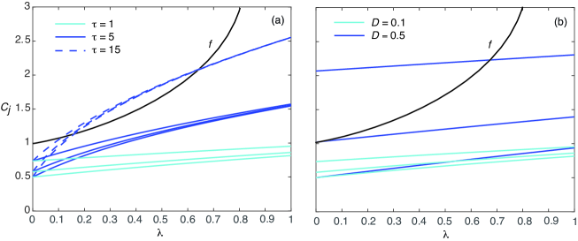
It follows from (i)-(iv) that if D<DN𝐷subscript𝐷𝑁D<D_{N} and τ𝜏\tau is sufficiently small (so that Cj(λ)superscriptsubscript𝐶𝑗𝜆C_{j}^{\prime}(\lambda) is sufficiently small), the curves f(λ)𝑓𝜆f(\lambda) and Cj(λ)subscript𝐶𝑗𝜆C_{j}(\lambda) will not intersect for any λ0𝜆0\lambda\geq 0. That is, the N𝑁N-spike solution is stable with respect to eigenmodes corresponding to real eigenvalues. The basic picture is illustrated in Fig. 4(a) for a 3-spike solution and D<D3𝐷subscript𝐷3D<D_{3}. One finds that there are no points of intersection for τ<τc𝜏subscript𝜏𝑐\tau<\tau_{c} with τc=O(10)subscript𝜏𝑐𝑂10\tau_{c}=O(10). On the other hand, for large τ𝜏\tau, there are two real eigenvalues for each j=1,2,3𝑗123j=1,2,3. It is clear that these eigenvalues do not appear by crossing the origin. Indeed, as highlighted in [34], instabilities induced by increasing τ𝜏\tau for fixed D𝐷D can only occur via a Hopf bifurcation. On the other hand, instabilities induced by increasing D𝐷D for fixed τ𝜏\tau can occur via a real eigenvalue entering the right half-plane, see Fig. 4(b).
Refer to caption
Figure 4: Plots of the functions Cj(λ)subscript𝐶𝑗𝜆C_{j}(\lambda), j=1,2,3𝑗123j=1,2,3, for a 3-spike solution of the classical GM model. (a) D=0.1<D3𝐷0.1subscript𝐷3D=0.1<D_{3}, and various τ𝜏\tau. (b) τ=0.1𝜏0.1\tau=0.1 and different diffusivities D𝐷D. For each triplet, the lowest curve is for C1subscript𝐶1C_{1} and the highest curve is for C3subscript𝐶3C_{3}. The black convex curve is the function f(λ)𝑓𝜆f(\lambda).

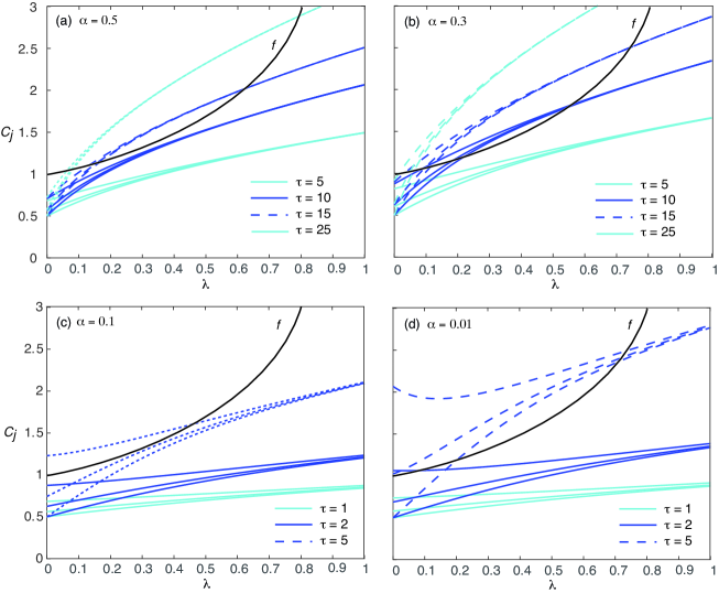
How does this story change for finite α𝛼\alpha and v2superscript𝑣2v^{2}? We will explore this issue by fixing the speed v𝑣v, and varying the switching rate α𝛼\alpha. This has two distinct effects. First, it modifies the effective diffusivity D=v2τ^𝐷superscript𝑣2^𝜏D=v^{2}\widehat{\tau} and, second, it alters the phase θλsubscript𝜃𝜆\theta_{\lambda}. For sufficiently large values of α𝛼\alpha, the time constant τ^^𝜏\widehat{\tau} is only weakly dependent on τ𝜏\tau so increasing the latter results in the appearance of pairs of positive real eigenvalues that do not cross the origin, indicative of a Hopf instability, see Fig. 5(a,b). On the other hand, in the limit α0𝛼0\alpha\rightarrow 0, we have τ^τ^𝜏𝜏\widehat{\tau}\approx\tau and the dominant effect of raising τ𝜏\tau is to increase the effective diffusivity. This implies that the resulting instability involves a real eigenvalue crossing the origin, as illustrated in Fig. 5(c,d). A necessary condition for no positive real eigenvalues is v2τ^<DNsuperscript𝑣2^𝜏subscript𝐷𝑁v^{2}\widehat{\tau}<D_{N}, that is, [v22αDN]τ<Dndelimited-[]superscript𝑣22𝛼subscript𝐷𝑁𝜏subscript𝐷𝑛[v^{2}-2\alpha D_{N}]\tau<D_{n}. The latter inequality is always satisfied if α>αc𝛼subscript𝛼𝑐\alpha>\alpha_{c} and holds for τ<τc(α)𝜏subscript𝜏𝑐𝛼\tau<\tau_{c}(\alpha) when α<αc𝛼subscript𝛼𝑐\alpha<\alpha_{c}, where

αc=v22DN;τc(α)=DNv22αDN for α<αc.formulae-sequencesubscript𝛼𝑐superscript𝑣22subscript𝐷𝑁subscript𝜏𝑐𝛼subscript𝐷𝑁superscript𝑣22𝛼subscript𝐷𝑁 for 𝛼subscript𝛼𝑐\alpha_{c}=\frac{v^{2}}{2D_{N}};\quad\tau_{c}(\alpha)=\frac{D_{N}}{v^{2}-2\alpha D_{N}}\mbox{ for }\alpha<\alpha_{c}. (65)

In the case N=3𝑁3N=3, we have D30.1subscript𝐷30.1D_{3}\approx 0.1 so that αc0.28subscript𝛼𝑐0.28\alpha_{c}\approx 0.28 when v2=0.1superscript𝑣20.1v^{2}=0.1. In cases where v2τ^<DNsuperscript𝑣2^𝜏subscript𝐷𝑁v^{2}\widehat{\tau}<D_{N}, we still require τ𝜏\tau to be sufficiently small so that there are no points of intersection with f(λ)𝑓𝜆f(\lambda).

Refer to caption
Figure 5: Plots of the functions Cj(λ)subscript𝐶𝑗𝜆C_{j}(\lambda), j=1,2,3𝑗123j=1,2,3, for a 3-spike solution of the hybrid reaction-transport model. Here v2=0.1superscript𝑣20.1v^{2}=0.1 and τ^=τ/(1+2τα)^𝜏𝜏12𝜏𝛼\widehat{\tau}=\tau/(1+2\tau\alpha). (a) α=0.5𝛼0.5\alpha=0.5; (b) α=0.3𝛼0.3\alpha=0.3; (c) α=0.1𝛼0.1\alpha=0.1 and (d) α=0.01𝛼0.01\alpha=0.01. In each case, the lowest curve is C1subscript𝐶1C_{1} and the highest curve is C3subscript𝐶3C_{3}.The black convex curve is the function f(λ)𝑓𝜆f(\lambda).

The next step is to look for pure imaginary eigenvalues. We begin by separating equation (61) into real and imaginary parts:

gj=gj,R+igj,I,f=fR+ifI,λ=λR+iλI.formulae-sequencesubscript𝑔𝑗subscript𝑔𝑗𝑅𝑖subscript𝑔𝑗𝐼formulae-sequence𝑓subscript𝑓𝑅𝑖subscript𝑓𝐼𝜆subscript𝜆𝑅𝑖subscript𝜆𝐼g_{j}=g_{j,R}+ig_{j,I},\quad f=f_{R}+if_{I},\quad\lambda=\lambda_{R}+i\lambda_{I}. (66)

If we now set λR=0subscript𝜆𝑅0\lambda_{R}=0, the eigenvalues along the imaginary axis are the solutions of the following pair of equations

g~j,R(λI)C~j,R(λI)f~R(λI),g~j,I(λI)C~j,I(λI)f~I(λI),formulae-sequencesubscript~𝑔𝑗𝑅subscript𝜆𝐼subscript~𝐶𝑗𝑅subscript𝜆𝐼subscript~𝑓𝑅subscript𝜆𝐼subscript~𝑔𝑗𝐼subscript𝜆𝐼subscript~𝐶𝑗𝐼subscript𝜆𝐼subscript~𝑓𝐼subscript𝜆𝐼\widetilde{g}_{j,R}(\lambda_{I})\equiv\widetilde{C}_{j,R}(\lambda_{I})-\widetilde{f}_{R}(\lambda_{I}),\quad\widetilde{g}_{j,I}(\lambda_{I})\equiv\widetilde{C}_{j,I}(\lambda_{I})-\widetilde{f}_{I}(\lambda_{I}), (67)

with C~j,R(λI)=Re[Cj(iλI)]subscript~𝐶𝑗𝑅subscript𝜆𝐼Redelimited-[]subscript𝐶𝑗𝑖subscript𝜆𝐼\widetilde{C}_{j,R}(\lambda_{I})=\mbox{Re}[C_{j}(i\lambda_{I})], C~j,L(λI)=Im[Cj(iλI)]subscript~𝐶𝑗𝐿subscript𝜆𝐼Imdelimited-[]subscript𝐶𝑗𝑖subscript𝜆𝐼\widetilde{C}_{j,L}(\lambda_{I})=\mbox{Im}[C_{j}(i\lambda_{I})], and

f~R(λI)subscript~𝑓𝑅subscript𝜆𝐼\displaystyle\widetilde{f}_{R}(\lambda_{I}) =Re[f(iλI)]=p(y)𝕃0[𝕃02+λI2]1p2(y)𝑑yp2(y)𝑑yabsentRedelimited-[]𝑓𝑖subscript𝜆𝐼superscriptsubscript𝑝𝑦subscript𝕃0superscriptdelimited-[]superscriptsubscript𝕃02superscriptsubscript𝜆𝐼21superscript𝑝2𝑦differential-d𝑦superscriptsubscriptsuperscript𝑝2𝑦differential-d𝑦\displaystyle=\mbox{Re}[f(i\lambda_{I})]=\frac{\int_{-\infty}^{\infty}p(y){\mathbb{L}}_{0}[{\mathbb{L}}_{0}^{2}+\lambda_{I}^{2}]^{-1}p^{2}(y)dy}{\int_{-\infty}^{\infty}\ p^{2}(y)dy}
f~I(λI)subscript~𝑓𝐼subscript𝜆𝐼\displaystyle\widetilde{f}_{I}(\lambda_{I}) =Im[f(iλI)]=λIp(y)[𝕃02+λI2]1p2(y)𝑑yp2(y)𝑑y.absentImdelimited-[]𝑓𝑖subscript𝜆𝐼subscript𝜆𝐼superscriptsubscript𝑝𝑦superscriptdelimited-[]superscriptsubscript𝕃02superscriptsubscript𝜆𝐼21superscript𝑝2𝑦differential-d𝑦superscriptsubscriptsuperscript𝑝2𝑦differential-d𝑦\displaystyle=\mbox{Im}[f(i\lambda_{I})]=\frac{\lambda_{I}\int_{-\infty}^{\infty}p(y)[{\mathbb{L}}_{0}^{2}+\lambda_{I}^{2}]^{-1}p^{2}(y)dy}{\int_{-\infty}^{\infty}\ p^{2}(y)dy}.

Without loss of generality, we can take λI0subscript𝜆𝐼0\lambda_{I}\geq 0. The following results for f~R(λI)subscript~𝑓𝑅subscript𝜆𝐼\widetilde{f}_{R}(\lambda_{I}) and f~I(λI)subscript~𝑓𝐼subscript𝜆𝐼\widetilde{f}_{I}(\lambda_{I}) hold [34]:

Refer to caption
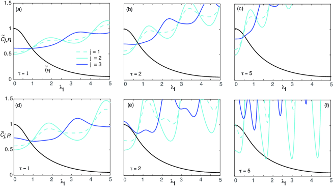
Figure 6: Plot of the functions C~j,R(λI)subscript~𝐶𝑗𝑅subscript𝜆𝐼\widetilde{C}_{j,R}(\lambda_{I}), j=1,2,3𝑗123j=1,2,3, for a 3-spike solution of the hybrid reaction-transport model. Here v2=0.1superscript𝑣20.1v^{2}=0.1 and τ^=τ/(1+2τα)^𝜏𝜏12𝜏𝛼\widehat{\tau}=\tau/(1+2\tau\alpha) with τ=1,2,5𝜏125\tau=1,2,5. (a-c) α=0.3𝛼0.3\alpha=0.3; (d-f) α=0.01𝛼0.01\alpha=0.01. The black curve is the function f~R(λI)subscript~𝑓𝑅subscript𝜆𝐼\widetilde{f}_{R}(\lambda_{I}).

(a) The function f~Rsubscript~𝑓𝑅\widetilde{f}_{R} has the asymptotic behavior

f~R(λI)1κcλI2+O(λI4) as λI0;f~R(λI)O(λI2) as λI,formulae-sequencesimilar-tosubscript~𝑓𝑅subscript𝜆𝐼1subscript𝜅𝑐superscriptsubscript𝜆𝐼2𝑂superscriptsubscript𝜆𝐼4 as subscript𝜆𝐼0subscript~𝑓𝑅subscript𝜆𝐼𝑂superscriptsubscript𝜆𝐼2 as subscript𝜆𝐼\widetilde{f}_{R}(\lambda_{I})\sim 1-\kappa_{c}\lambda_{I}^{2}+O(\lambda_{I}^{4})\mbox{ as }\lambda_{I}\rightarrow 0;\quad\widetilde{f}_{R}(\lambda_{I})\rightarrow O(\lambda_{I}^{-2})\mbox{ as }\lambda_{I}\rightarrow\infty, (68)

where κc>0subscript𝜅𝑐0\kappa_{c}>0. Moreover, f𝑓f is a strictly monotonically decreasing function for all 0<λI<0subscript𝜆𝐼0<\lambda_{I}<\infty, that is, f~R(λI)<0superscriptsubscript~𝑓𝑅subscript𝜆𝐼0\widetilde{f}_{R}^{\prime}(\lambda_{I})<0.

(b) The function f~Isubscript~𝑓𝐼\widetilde{f}_{I} has the asymptotic behavior

f~I(λI)34λI+O(λI3) as λI0;f~I(λI)O(λI1) as λI,formulae-sequencesimilar-tosubscript~𝑓𝐼subscript𝜆𝐼34subscript𝜆𝐼𝑂superscriptsubscript𝜆𝐼3 as subscript𝜆𝐼0subscript~𝑓𝐼subscript𝜆𝐼𝑂superscriptsubscript𝜆𝐼1 as subscript𝜆𝐼\widetilde{f}_{I}(\lambda_{I})\sim\frac{3}{4}\lambda_{I}+O(\lambda_{I}^{3})\mbox{ as }\lambda_{I}\rightarrow 0;\quad\widetilde{f}_{I}(\lambda_{I})\rightarrow O(\lambda_{I}^{-1})\mbox{ as }\lambda_{I}\rightarrow\infty, (69)

and f~I(λI)>0subscript~𝑓𝐼subscript𝜆𝐼0\widetilde{f}_{I}(\lambda_{I})>0 for all 0<λI<0subscript𝜆𝐼0<\lambda_{I}<\infty.

Again we begin by considering the classical GM model in the limit αinfty𝛼𝑖𝑛𝑓𝑡𝑦\alpha\rightarrow infty and v𝑣v\rightarrow\infty with D𝐷D fixed. Note that C~j,R(0)=Cj(0)=Bj(D)subscript~𝐶𝑗𝑅0subscript𝐶𝑗0subscript𝐵𝑗𝐷\widetilde{C}_{j,R}(0)=C_{j}(0)=B_{j}(D) for all λIsubscript𝜆𝐼\lambda_{I}. Hence, if D<DN𝐷subscript𝐷𝑁D<D_{N} then C~j,R(0)<f~R(0)subscript~𝐶𝑗𝑅0subscript~𝑓𝑅0\widetilde{C}_{j,R}(0)<\widetilde{f}_{R}(0). Moreover, if τ>0𝜏0\tau>0 then C~j,R(λI)subscript~𝐶𝑗𝑅subscript𝜆𝐼\widetilde{C}_{j,R}(\lambda_{I}) is an increasing function of λIsubscript𝜆𝐼\lambda_{I} [34], which from result (a) means that there is a single intersection point with f^R(λI)subscript^𝑓𝑅subscript𝜆𝐼\widehat{f}_{R}(\lambda_{I}) and thus a unique positive root λIsuperscriptsubscript𝜆𝐼\lambda_{I}^{*} where g~j,R(λI)=0subscript~𝑔𝑗𝑅superscriptsubscript𝜆𝐼0\widetilde{g}_{j,R}(\lambda_{I}^{*})=0. Moreover, from result (b) we have f~I(λI)>0subscript~𝑓𝐼subscript𝜆𝐼0\widetilde{f}_{I}(\lambda_{I})>0 for all λI>0subscript𝜆𝐼0\lambda_{I}>0, whereas C~j,I=O(τ)subscript~𝐶𝑗𝐼𝑂𝜏\widetilde{C}_{j,I}=O(\tau) as τ0𝜏0\tau\rightarrow 0. This implies that for sufficiently small τ𝜏\tau, g~j,I(λI)<0subscript~𝑔𝑗𝐼superscriptsubscript𝜆𝐼0\widetilde{g}_{j,I}(\lambda_{I}^{*})<0 and there are no purely imaginary eigenvalues.

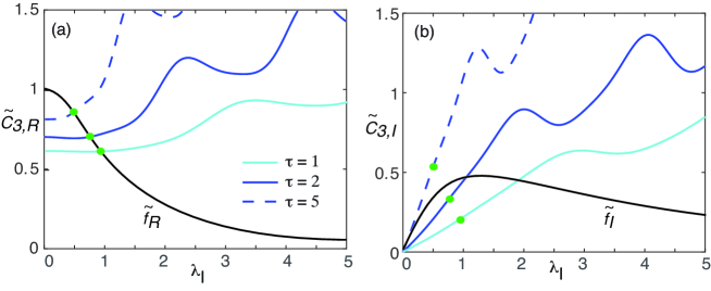
Now suppose that α𝛼\alpha and v𝑣v are finite. Similar to the case of real eigenvalues, we wish to explore how C~j,R(λI)subscript~𝐶𝑗𝑅subscript𝜆𝐼\widetilde{C}_{j,R}(\lambda_{I}) and C~j,I(λI)subscript~𝐶𝑗𝐼subscript𝜆𝐼\widetilde{C}_{j,I}(\lambda_{I}) depend on the switching rate α𝛼\alpha. Some example plots of C~j,R(λI)subscript~𝐶𝑗𝑅subscript𝜆𝐼\widetilde{C}_{j,R}(\lambda_{I}) are shown in Fig. 6 for the two cases α=0.3𝛼0.3\alpha=0.3 and α=0.01𝛼0.01\alpha=0.01. It is clear that C~j,R(λI)subscript~𝐶𝑗𝑅subscript𝜆𝐼\widetilde{C}_{j,R}(\lambda_{I}) is no longer a monotonically increasing function of λIsubscript𝜆𝐼\lambda_{I}, even though C~j,R(λI)subscript~𝐶𝑗𝑅subscript𝜆𝐼\widetilde{C}_{j,R}(\lambda_{I})\rightarrow\infty as λIsubscript𝜆𝐼\lambda_{I}\rightarrow\infty.That is, there still exists at least one intersection point between C~j,R(λI)subscript~𝐶𝑗𝑅subscript𝜆𝐼\widetilde{C}_{j,R}(\lambda_{I}) and f~R(λI)subscript~𝑓𝑅subscript𝜆𝐼\widetilde{f}_{R}(\lambda_{I}), but it is no longer necessarily unique unless τ𝜏\tau is sufficiently small; the latter condition ensures that the curves are only weakly non-monotonic. For larger values of τ𝜏\tau, one has to investigate the number of intersection points numerically. Although we cannot make any rigorous statements, our numerical studies suggest that there is a unique intersection point for all τ>0𝜏0\tau>0 when α>αc𝛼subscript𝛼𝑐\alpha>\alpha_{c}, as illustrated in Fig. 6(a-c). On the other hand, for α<αc𝛼subscript𝛼𝑐\alpha<\alpha_{c} and sufficiently large τ𝜏\tau, it is possible for C~j,R(λI)subscript~𝐶𝑗𝑅subscript𝜆𝐼\widetilde{C}_{j,R}(\lambda_{I}) to intersect f~R(λI)subscript~𝑓𝑅subscript𝜆𝐼\widetilde{f}_{R}(\lambda_{I}) more than once, see Fig. 6(d-f).

Refer to caption
Figure 7: Plot of the functions (a) C~3,R(λI)subscript~𝐶3𝑅subscript𝜆𝐼\widetilde{C}_{3,R}(\lambda_{I}) and (b) C~3,I(λI)subscript~𝐶3𝐼subscript𝜆𝐼\widetilde{C}_{3,I}(\lambda_{I}) for a 3-spike solution of the hybrid reaction-transport model. Here v2=0.1superscript𝑣20.1v^{2}=0.1 and τ^=τ/(1+2τα)^𝜏𝜏12𝜏𝛼\widehat{\tau}=\tau/(1+2\tau\alpha) with τ=1,2,5𝜏125\tau=1,2,5 and α=0.3𝛼0.3\alpha=0.3. The black curves in (a) and (b) are the functions f~R(λI)subscript~𝑓𝑅subscript𝜆𝐼\widetilde{f}_{R}(\lambda_{I}) and f~I(λI)subscript~𝑓𝐼subscript𝜆𝐼\widetilde{f}_{I}(\lambda_{I}), respectively. Green dots indicate the values at λI=λIsubscript𝜆𝐼superscriptsubscript𝜆𝐼\lambda_{I}=\lambda_{I}^{*}.
Refer to caption
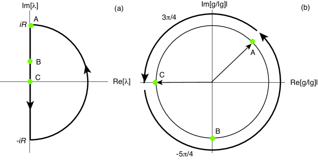
Figure 8: Winding number argument of [34]. (a) Counterclockwise path along the contour ΓRΓIΓ¯IsubscriptΓ𝑅subscriptΓ𝐼subscript¯Γ𝐼\Gamma_{R}\cup\Gamma_{I}\cup\overline{\Gamma}_{I} in the complex λ𝜆\lambda-plane, where ΓRsubscriptΓ𝑅\Gamma_{R} is the semi-circle of radius R𝑅R, ΓI=[iR,0]subscriptΓ𝐼𝑖𝑅0\Gamma_{I}=[iR,0] and Γ¯I=[0,iR]subscript¯Γ𝐼0𝑖𝑅\overline{\Gamma}_{I}=[0,-iR]. (b) Change in argg𝑔\arg g along ΓIsubscriptΓ𝐼\Gamma_{I} (from A to C) in the limit R𝑅R\rightarrow\infty. There exists a unique point iλ𝑖superscript𝜆i\lambda^{*} on the positive imaginary axis where g~j,R(λ)=0subscript~𝑔𝑗𝑅superscript𝜆0\widetilde{g}_{j,R}(\lambda^{*})=0 (point B). If g~I(λ)<0subscript~𝑔𝐼superscript𝜆0\widetilde{g}_{I}(\lambda^{*})<0 then argg(iλ)=π/2𝑔𝑖superscript𝜆𝜋2\arg g(i\lambda^{*})=-\pi/2 and Δargg=5π/4Δ𝑔5𝜋4\Delta\arg g=-5\pi/4.

For the moment, take α>αc𝛼subscript𝛼𝑐\alpha>\alpha_{c} and assume that for the given τ𝜏\tau there exists a unique point iλI𝑖superscriptsubscript𝜆𝐼i\lambda_{I}^{*} on the imaginary axis at which g~j,R(λI)=0subscript~𝑔𝑗𝑅superscriptsubscript𝜆𝐼0\widetilde{g}_{j,R}(\lambda_{I}^{*})=0. It can be checked that if τ𝜏\tau is sufficiently small then g~j,I(λI)<0subscript~𝑔𝑗𝐼superscriptsubscript𝜆𝐼0\widetilde{g}_{j,I}(\lambda_{I}^{*})<0. This is illustrated in Fig. 7, where we plot C~3,R(λI)subscript~𝐶3𝑅subscript𝜆𝐼\widetilde{C}_{3,R}(\lambda_{I}) and C~3,I(λI)subscript~𝐶3𝐼subscript𝜆𝐼\widetilde{C}_{3,I}(\lambda_{I}) for α=0.3𝛼0.3\alpha=0.3 and various τ𝜏\tau. As τ𝜏\tau increases the curve C~3,R(λI)subscript~𝐶3𝑅subscript𝜆𝐼\widetilde{C}_{3,R}(\lambda_{I}) becomes steeper in a neighborhood of the origin so that g~j,I(λI)subscript~𝑔𝑗𝐼superscriptsubscript𝜆𝐼\widetilde{g}_{j,I}(\lambda_{I}^{*}) switches sign. The condition g~j,I(λI)<0subscript~𝑔𝑗𝐼superscriptsubscript𝜆𝐼0\widetilde{g}_{j,I}(\lambda_{I}^{*})<0 not only ensures that there are no pure imaginary eigenvalues but also implies that there are no complex-valued eigenvalues in the right complex half-plane. This follows from the winding number construction of [34]. First, recall the argument principle of complex analysis: if F(x)𝐹𝑥F(x) is a meromorphic function inside and on some closed contour C𝐶C and F𝐹F has no zeros or poles on C𝐶C, then

12πiCF(z)F(z)𝑑z=12πiF(C)dww=ZP,12𝜋𝑖subscriptcontour-integral𝐶superscript𝐹𝑧𝐹𝑧differential-d𝑧12𝜋𝑖subscriptcontour-integral𝐹𝐶𝑑𝑤𝑤𝑍𝑃\frac{1}{2\pi i}\oint_{C}\frac{F^{\prime}(z)}{F(z)}dz=\frac{1}{2\pi i}\oint_{F(C)}\frac{dw}{w}=Z-P, (70)

where w=F(z)𝑤𝐹𝑧w=F(z), and Z,P𝑍𝑃Z,P denote, respectively, the number of zeros (including multiplicity) and poles (including order) of F(z)𝐹𝑧F(z) inside C𝐶C. The second integral is the winding number of F𝐹F. Consider the contour C𝐶C shown in Fig. 8(a), which consists of the semicircle ΓRsubscriptΓ𝑅\Gamma_{R} given by |λ|=R>0𝜆𝑅0|\lambda|=R>0 for π/2argλπ/2𝜋2arg𝜆𝜋2-\pi/2\mbox{arg}\lambda\leq\pi/2, and the section iRIm[λ]iR𝑖𝑅Imdelimited-[]𝜆𝑖𝑅-iR\leq\mbox{Im}[\lambda]\leq iR of the imaginary axis. Assuming that α𝛼\alpha is sufficiently large so that there are no pure imaginary eigenvalues (see above), we can let R𝑅R\rightarrow\infty and use the argument principle to determine the number of zeros of gj(λ)subscript𝑔𝑗𝜆g_{j}(\lambda) in the right-half plane. Since Cj(λ)λ1/2similar-tosubscript𝐶𝑗𝜆superscript𝜆12C_{j}(\lambda)\sim\lambda^{1/2} as |λ|𝜆|\lambda|\rightarrow\infty while f(λ)0𝑓𝜆0f(\lambda)\rightarrow 0 as |λ|𝜆|\lambda|\rightarrow\infty, it follows that argλ𝜆\arg\lambda changes by an amount π/2𝜋2\pi/2 as ΓRsubscriptΓ𝑅\Gamma_{R} is traversed counterclockwise. Using the fact that gj(λ)subscript𝑔𝑗𝜆g_{j}(\lambda) is analytic in the right-half plane, except at the simple pole λ=ν0>0𝜆subscript𝜈00\lambda=\nu_{0}>0 (P=1𝑃1P=1), it follows from the argument principle that the number M𝑀M of zeros of gj(λ)subscript𝑔𝑗𝜆g_{j}(\lambda) in the right half-plane is

Z=54+1π[arggj]ΓI,𝑍541𝜋subscriptdelimited-[]subscript𝑔𝑗subscriptΓ𝐼Z=\frac{5}{4}+\frac{1}{\pi}[\arg g_{j}]_{\Gamma_{I}}, (71)

where [arggj]ΓIsubscriptdelimited-[]subscript𝑔𝑗subscriptΓ𝐼[\arg g_{j}]_{\Gamma_{I}} is the change in the argument of g𝑔g along the semi-infinite imaginary axis ΓI=iλsubscriptΓ𝐼𝑖𝜆\Gamma_{I}=i\lambda, 0λ<0𝜆0\leq\lambda<\infty. Setting C~j(λ)=Cj(iλ)subscript~𝐶𝑗𝜆subscript𝐶𝑗𝑖𝜆\widetilde{C}_{j}(\lambda)=C_{j}(i\lambda) with λ𝜆\lambda real, we have C~j(λ)iλsimilar-tosubscript~𝐶𝑗𝜆𝑖𝜆\widetilde{C}_{j}(\lambda)\sim\sqrt{i\lambda} as λ𝜆\lambda\rightarrow\infty so that argg=π/4𝑔𝜋4\arg g=\pi/4 at the start of ΓIsubscriptΓ𝐼\Gamma_{I}. Moreover, arggj(0)=πsubscript𝑔𝑗0𝜋\arg g_{j}(0)=\pi, since gj(0)=Cj(0)f(0)<0subscript𝑔𝑗0subscript𝐶𝑗0𝑓00g_{j}(0)=C_{j}(0)-f(0)<0. Given the unique point iλ𝑖superscript𝜆i\lambda^{*} on the positive imaginary axis where g~j,R(λ)=0subscript~𝑔𝑗𝑅superscript𝜆0\widetilde{g}_{j,R}(\lambda^{*})=0. If we can show that g~j,I(λ)<0subscript~𝑔𝑗𝐼superscript𝜆0\widetilde{g}_{j,I}(\lambda^{*})<0, then argg(iλ)=π/2𝑔𝑖superscript𝜆𝜋2\arg g(i\lambda^{*})=-\pi/2 and the change of argg𝑔\arg g along ΓIsubscriptΓ𝐼\Gamma_{I} is 5π/45𝜋4-5\pi/4, see Fig. 8(b). Equation (71) then ensures that there are no eigenvalues in the right half-plane and the N𝑁N-spike solution is stable. From result (b), we have f~I(λ)>0subscript~𝑓𝐼𝜆0\widetilde{f}_{I}(\lambda)>0 for all 0<λ<0𝜆0<\lambda<\infty, whereas C~j,I(0)=0subscript~𝐶𝑗𝐼00\widetilde{C}_{j,I}(0)=0 and C~j,I(λ)=O(τ)subscript~𝐶𝑗𝐼𝜆𝑂𝜏\widetilde{C}_{j,I}(\lambda)=O(\tau) as τ0𝜏0\tau\rightarrow 0 for finite λ𝜆\lambda. Hence, for j=1,,N𝑗1𝑁j=1,\ldots,N, there exists a τ0>0subscript𝜏00\tau_{0}>0 such that g~j,I(λ)<0subscript~𝑔𝑗𝐼superscript𝜆0\widetilde{g}_{j,I}(\lambda^{*})<0 and thus Z=0𝑍0Z=0 for all τ𝜏\tau satisfying 0τ<τ00𝜏subscript𝜏00\leq\tau<\tau_{0}.

We have thus established that the hybrid reaction-transport model with GM kinetics supports a stable N𝑁N-spike solution that is stable on O(1)𝑂1O(1) time-scales provided that α>αc𝛼subscript𝛼𝑐\alpha>\alpha_{c} and 0τ<τ00𝜏subscript𝜏00\leq\tau<\tau_{0} for some τ0=τ0(α)subscript𝜏0subscript𝜏0𝛼\tau_{0}=\tau_{0}(\alpha). The first condition ensures that D=v2τ^<DN𝐷superscript𝑣2^𝜏subscript𝐷𝑁D=v^{2}\widehat{\tau}<D_{N}, with DNsubscript𝐷𝑁D_{N} given by equation (36). When τ𝜏\tau increases beyond τ0subscript𝜏0\tau_{0}, a pair of complex conjugate eigenvalues crosses into the right half-plane, indicating the occurrence of a Hopf bifurcation. Finally, note that if α<αc𝛼subscript𝛼𝑐\alpha<\alpha_{c}, then the same winding number argument can be used to show that an N𝑁N-spike is still stable for sufficiently small τ𝜏\tau, but the nature of the instability as τ𝜏\tau increases differs. This is due to the fact that D𝐷D crosses the critical value DNsubscript𝐷𝑁D_{N}, signaling that a real eigenvalue passes the origin into the right half-plane. An example of such a scenario is shown in Fig. 9.
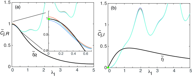
Refer to caption
Figure 9: Plot of the functions (a) C~3,R(λ)subscript~𝐶3𝑅𝜆\widetilde{C}_{3,R}(\lambda) and (b) C~3,I(λ)subscript~𝐶3𝐼𝜆\widetilde{C}_{3,I}(\lambda) for a 3-spike solution of the hybrid reaction-transport model. Here v2=0.1superscript𝑣20.1v^{2}=0.1 and τ^=τ/(1+2τα)^𝜏𝜏12𝜏𝛼\widehat{\tau}=\tau/(1+2\tau\alpha) with τ=2𝜏2\tau=2. Solutions for three slightly different values of the switching rate are shown: α=0.02,0.025,0.03𝛼0.020.0250.03\alpha=0.02,0.025,0.03. As α𝛼\alpha increases, C~3,R(λ)subscript~𝐶3𝑅𝜆\widetilde{C}_{3,R}(\lambda) crosses f~R(λ)subscript~𝑓𝑅𝜆\widetilde{f}_{R}(\lambda) at the origin (highlighted by the green dot in the inset), indicating that a real eigenvalue becomes positive. For a narrow range of α𝛼\alpha there exists a pair of intersection points between C~3,R(λ)subscript~𝐶3𝑅𝜆\widetilde{C}_{3,R}(\lambda) and f~R(λ)subscript~𝑓𝑅𝜆\widetilde{f}_{R}(\lambda).

5 Conclusion

In summary, we have extended the asymptotic analysis of the classical two-component GM model [32, 34] to a hybrid reaction-transport model with GM kinetics in order to derive conditions for the existence and stability of an N𝑁N-spike solution. We exploited the fact that in the limit α𝛼\alpha\rightarrow\infty and v𝑣v\rightarrow\infty with D=v2/(μ2+2α)𝐷superscript𝑣2subscript𝜇22𝛼D=v^{2}/(\mu_{2}+2\alpha) fixed, the 3-component hybrid reaction-transport model reduces to the classical two-component GM reaction-diffusion model with effective inhibitor diffusivity D𝐷D. Here v𝑣v is the speed of active transport, α𝛼\alpha is the switching rate and μ2subscript𝜇2\mu_{2} is the degradation rate of the inhibitor. Linearizing about a multi-spike solution resulted in a non-local eigenvalue problem that could be used to derive stability conditions as a function of the switching rate α𝛼\alpha. In particular, we showed that there exists a critical switching rate αcsubscript𝛼𝑐\alpha_{c} such that for α>αc𝛼subscript𝛼𝑐\alpha>\alpha_{c}, the multi-spike solution tends to undergo a Hopf instability, whereas for α<αc𝛼subscript𝛼𝑐\alpha<\alpha_{c} the instability is due to one or more real eigenvalues becoming positive. Although we focused our analysis on the particular hybrid model introduced within the context of synaptogenesis in C. elegans [29, 30], it would be interesting in future work to explore a more general class of hybrid models. One generalization would be to consider alternative reaction schemes to GM kinetics, where it is not possible to reduce the steady-state equations to a two-component reaction-diffusion system by eliminating the flux J=v(A+A)𝐽𝑣subscript𝐴subscript𝐴J=v(A_{+}-A_{-}). This would require modifying the construction of multi-spike solutions in section 3. A second modification would be to allow for biased active transport by taking the speeds of the left-moving and right-moving states to differ. Any effective reduction of the hybrid model would result in an advection-diffusion equation for the inhibitor. Third, from a mathematical perspective, there is no reason to identify the activator as the diffusing species and the inhibitor as the actively transported species. How would the results change if the transport modes of the activator and inhibitor were reversed?

The particular application of the hybrid model to larval development also raises a number of issues. For example, while the important role of CaMKII in regulating the delivery of GLR-1 to synapses along the ventral cord of C. elegans is well known, the detailed mechanisms regarding their interactions are still unclear. Developing a more detailed biophysical model of CaMKII-GLR-1 coupling would be one way to explore more general reaction schemes in the hybrid model. This might also require the introduction of additional components, such as allowing for stationary states of GLR-1 and distinguishing between cytoplasmic and membrane-bound CaMKII. Another major aspect of C. elegans development is the insertion of new synaptic puncta as the larva grow, see Fig. 1. It would be interesting to model this as an example of spike insertion in a growing domain.


References

  • [1] Turing AM. 1952. The chemical basis of morphogenesis. Philos Trans Roy Soc Lond Ser B Biol Sci 237 37-72.
  • [2] Gierer A, Meinhardt H. 1972 A theory of biological pattern formation. Kybernetik 12 30-39.
  • [3] Zaikin AN, Zhabotinsky AM. 1970. Concentration wave propagation in two-dimensional liquid-phase self-oscillating system. Nature 225, 535-537.
  • [4] Kondo S, Asai R. 1995. A reaction-diffusion wave on the skin of the marine angelfish Pomacanthus. Nature 376 765-768.
  • [5] Murray JD. 2001. Mathematical Biology. II Spatial Models and Biomedical Applications, Interdisciplinary Applied Mathematics V. 18, Springer-Verlag, New York.
  • [6] Cross MC, Greenside HS. 2009. Pattern formation and dynamics in non-equilibrium systems. Cambridge: Cambridge University Press.
  • [7] Walgraef D. 1997. Pattern Formation with Examples from Physics, Chemistry, and Materials Science. New York: Springer
  • [8] Levin SA. 1992. The problem of pattern and scale in ecology. Ecology 73 1943-1967.
  • [9] Rietkerk M, van de Koppel J. 2007. Regular pattern formation in real ecosystems. Trends. Ecol. Evol. 23 169-175.
  • [10] Ermentrout GB, Cowan JD. 1979. A mathematical theory of visual hallucination patterns. Bio. Cybern. 34 137-150.
  • [11] Bressloff PC, Cowan JD, Golubitsky M, Thomas PJ, Wiener M. 2001 Geometric Visual Hallucinations, Euclidean Symmetry and the Functional Architecture of Striate Cortex. Phil. Trans. Roy. Soc. Lond. B 356 299-330
  • [12] Kholodenko BN. 2009. Spatially distributed cell signalling. FEBS Letters 583 4006-4012.
  • [13] Howard M. 2012. How to build a robust intracellular concentration gradient. Trends Cell Biol. 22 311-317.
  • [14] Goryachev AB, Pokhilko AV. 2008. Dynamics of Cdc42 network embodies a Turing-type mechanism of yeast cell polarity. FEBS Lett 582 1437-1443.
  • [15] Drake T, Vavylonis D. 2010. Cytoskeletal dynamics in fission yeast: a review of models for polarization and division. HFSP journal 4 122-130.
  • [16] Ishihara S, Otsuji M, Mochizuki A. 2007. Transient and steady state of mass-conserved reaction-diffusion systems. Phys. Rev. E 75 015203(R).
  • [17] Otsuji M., Ishihara S, Co C, Kaibuchi K, Mochizuki A, Kuroda S. 2007. A mass conserved reaction-diffusion system captures properties of cell polarity. PLoS Comput Biol. 3 e108.
  • [18] Brauns F, Halatek J, Frey E. Phase-space geometry of reaction-diffusion dynamics. arXiv:1812.08684 (2020).
  • [19] Halatek J. Brauns F, Frey E. 2018. Self-organization principles of intracellular pattern formation. Phil. Trans. R. Soc. B 373 20170107.
  • [20] Halatek J, Frey E. 2018. Rethinking pattern formation in reaction-diffusion systems. Nat. Phys. 14 507-514.
  • [21] Hofmann A, Makela J, Sherratt D J, Heermann D, Murray SM. 2019. Self-organised segregation of bacterial chromosomal origins. eLife 8 e46564.
  • [22] Murray SM, Sourjik V. 2017. Self-organization and positioning of bacterial protein clusters. Nature Phys. 13 1006-1013.
  • [23] Subramanian S, Murray SM. 2020. Pattern selection in reaction diffusion systems. arXiv:2005.07940v2.
  • [24] Rongo C and Kaplan JM. 1999 CaMKII regulates the density of central glutamatergic synapses in vivo. Nature 402 195-199.
  • [25] Shen K, Meyer T. 1999. Dynamic control of CaMKII translocation and localization in hippocampal neurons by NMDA receptor stimulation. Science 284 162-166.
  • [26] Monteiro MI, Ahlawat S, Kowalski JR, Malkin E, Koushika SP, Juoa P. 2012. The kinesin-3 family motor KLP-4 regulates anterograde trafficking of GLR-1 glutamate receptors in the ventral nerve cord of Caenorhabditis elegans. Mol Biol Cell 23 3647-3662.
  • [27] Hoerndli FJ, Maxfield DA, Brockie PJ, Mellem JE, Jensen E, Wang R, Madsen DM, and Maricq AV. 2013. Kinesin-1 regulates synaptic strength by mediating the delivery, removal, and redistribution of AMPA receptors. Neuron 80 1421-1437.
  • [28] Hoerndli FJ, Wang R, Mellem JE, Kallarackal A, Brockie PJ, Thacker C, Jensen E, Madsen DM, and Maricq AV. 2015. Neuronal activity and CaMKII regulate kinesin-mediated transport of synaptic AMPARs. Neuron 86 457-474.
  • [29] Brooks HA and Bressloff PC. 2016. A mechanism for Turing pattern formation with active and passive transport. SIAM J Appl Dyn Syst 15 1823-1843.
  • [30] Brooks HA and Bressloff PC. 2017. Turing mechanism for homeostatic control of synaptic density during C. elegans growth. Phys Rev E 96 012413.
  • [31] Hillen T. 1996. A Turing model with correlated random walk. J Math Biol 35 49-72.
  • [32] Iron D. Ward MJ, Wei J. 2001. The stability of spike solutions to the one-dimensional Gierer-Meinhardt model. Physica D 150 25-62.
  • [33] Iron D, Ward MJ. 2002 The Dynamics of multi-spike solutions for the one-dimensional Gierer-Meinhardt model. SIAM J. Appl. Math. 62 1924-1951.
  • [34] Ward MJ, Wei J. 2003. Hopf bifurcation and oscillatory instabilities of spike solutions for the one-dimensional Gierer-Meinhardt model. J. Nonlinear Science 13 209-264.
  • [35] Kolokolnikov T, Ward MJ, Wei J. 2005. The existence and stability of spike equilibria in the one-dimensional Gray-Scott model: The low feed rate regime. Studies in Appl. Math. 115 21-71.
  • [36] Kolokolnikov T, Ward MJ, Wei J. 2005. The existence and stability of spike equilibria in the one-dimensional Gray-Scott model: The pulse-splitting regime. Studies in Appl. Math. 115 258-293.
  • [37] Tzou J, Nec Y, Ward MJ. 2013. The stability of localized spikes for the 1-D Brusselator reaction-diffusion model. Eur. J. Appl. Math. 24 515.
  • [38] Kac M. 1974. Rocky Mountain J. Math 4 497.