Lefschetz fibrations with arbitrary signature

R. İnanç Baykur Department of Mathematics and Statistics, University of Massachusetts, Amherst, MA 01003, USA baykur@math.umass.edu  and  Noriyuki Hamada Department of Mathematics and Statistics, University of Massachusetts, Amherst, MA 01003, USA hamada@math.umass.edu
Abstract.

We develop techniques to construct explicit symplectic Lefschetz fibrations over the 222–sphere with any prescribed signature σ𝜎\sigma and any spin type when σ𝜎\sigma is divisible by 161616. This solves a long-standing conjecture on the existence of such fibrations with positive signature. As applications, we produce symplectic 444–manifolds that are homeomorphic but not diffeomorphic to connected sums of S2×S2superscript𝑆2superscript𝑆2S^{2}\times S^{2}, with the smallest topology known to date, as well as larger examples as symplectic Lefschetz fibrations.

1. Introduction

An immense literature has been dedicated to the study of symplectic Lefschetz fibrations since the works of Donaldson and Gompf [19, 31] have established Lefschetz fibrations over the 222–sphere as topological counter-parts of closed symplectic 444–manifolds, after blow-ups. However, the possible values of one of the most fundamental invariants of 444–manifolds, the signature of a Lefschetz fibration over the 222–sphere, has not been quite understood, despite many effective ways of calculating it being available, due to the works of Endo, Ozbagci and others [42, 20, 21, 45, 51, 17]. The aim of our article is to resolve this problem:

Theorem A.

There exist infinitely many relatively minimal symplectic Lefschetz fibrations over the 222–sphere, whose total spaces have any prescribed signature σ𝜎\sigma\in\mathbb{Z} and any spin type when σ𝜎\sigma is divisible by 161616. All the examples can be chosen to be simply-connected, minimal, and with fiber genus as small as 999, as well as arbitrarily high.

Fiber summing with trivial fibrations over orientable surfaces, possibly with boundary, the main statements of the theorem carry over to Lefschetz fibrations over any compact orientable surface.

It was often conjectured that Lefschetz fibrations over the 222–sphere with positive signatures did not exist, which constituted a long-standing open problem; see e.g. [44, 45], [56], [57, Problems 6.3, 6.4], [38, Problems 7.4, 7.5]. Our examples settle this conjecture in the negative. In contrast, in the literature there are plenty of examples of Lefschetz fibrations over the 222–sphere with negative signatures, many coming from algebraic geometry. To the best of our knowledge, even in this case it was not known that every negative signature could be realized; see Remark 18.

We will prove the theorem by explicitly describing the Lefschetz fibrations in terms of their monodromy factorizations, which correspond to positive Dehn twist factorizations in the mapping class group of an orientable surface. Our constructions will heavily use variations of the breeding technique [12, 32] for building Lefschetz pencils and fibrations out of lower genera ones. A great deal of our efforts will be spent on building monodromy factorizations for spin Lefschetz fibrations. We should note that, even though we effectively use the breeding technique to derive new symplectic 444–manifolds from smaller ones, this is not an inherently symplectic operation; we build pencils/fibrations with locally non-complex nodal singularities in intermediate steps, but then we match all the locally non-complex nodes with locally complex ones and remove these pairs at the end (which corresponds to a 555–dimensional 333–handle attachment, and at times to removing an S2×S2superscript𝑆2superscript𝑆2S^{2}\times S^{2} summand from a connected sum); see Remark 16.

We should also note that more flexible variations of this signature realization problem are easier to address, even in the holomorphic category: For Lefschetz pencils, where one allows base points, examples with prescribed signatures are easy to obtain using very ample line bundles on suitable compact complex surfaces. Similarly, there are many compact complex surfaces admitting semi-stable fibrations over non-rational complex curves; in fact, when one allows the base surface of the fibration to be of higher genera, there are even smooth fibrations, often called Kodaira fibrations, whose total spaces have positive signatures. While the essential challenge is to describe positive signature Lefschetz fibrations over the 222–sphere, we shall point out that most, and possibly all, of our examples in Theorem A are not holomorphic; see Remark 19. Since there are no separating vanishing cycles in our fibrations, by Endo’s signature formula [20], none of our examples with non-negative signatures can be hyperelliptic either.

Recall that two 444–manifolds are said to be stably diffeomorphic if they become diffeomorphic after taking connected sums of each with copies of S2×S2superscript𝑆2superscript𝑆2S^{2}\times S^{2}. By a classical result of C. T. C. Wall, we have the following immediate corollary to our theorem:

Corollary B.

Any closed smooth oriented simply-connected 444–manifold is stably diffeomorphic to a symplectic Lefschetz fibration.

Furthermore, by crafting the monodromies of our fibrations more carefully and invoking Freedman’s celebrated work, we can show that any closed smooth oriented simply-connected 444–manifold X𝑋X with signature σ𝜎\sigma, provided its holomorphic Euler charactersitic χh(X):=14(e(X)+σ(X))assignsubscript𝜒𝑋14e𝑋𝜎𝑋\chi_{h}(X):=\frac{1}{4}({\text{e}}(X)+\sigma(X)) is integral and sufficiently large (depending solely on σ𝜎\sigma), is homeomorphic to a symplectic Lefschetz fibration. (Doing this for all integral χh(X)subscript𝜒𝑋\chi_{h}(X) greater than a constant that depends on σ𝜎\sigma requires more work.) So we get symplectic Lefschetz fibrations as exotic copies of standard 444–manifolds that are connected sums of copies of S2×S2superscript𝑆2superscript𝑆2S^{2}\times S^{2}, 2{\mathbb{CP}}{}^{2} and the K3K3{\rm K3} surface, taken with either orientations. It is a very interesting problem to determine the smallest χhsubscript𝜒\chi_{h} (or b2subscript𝑏2b_{2}) one can take for a given σ𝜎\sigma. For example, when σ=0𝜎0\sigma=0, we can show that:

Corollary C.

There exist symplectic Lefschetz fibrations, whose total spaces are pairwise non-diffeomorphic, but homeomorphic to #m(S2×S2)subscript#𝑚superscript𝑆2superscript𝑆2\#_{m}(S^{2}\times S^{2}), where the examples can be chosen so that m𝑚m is as small as 127127127, or is any odd m415𝑚415m\geq 415.

These are the first exampes of Lefschetz fibrations in the given homeomorphism classes. The spin examples are particularly interesting, and have been sought after for quite some time, in connection with the existence of exotically knotted orientable surfaces in the 444–sphere. Examples of exotically knotted non-orientable surfaces in the 444–sphere were constructed by Finashin, Kreck and Viro [24], and further examples were given by Finashin [23], all using involutions on genus–111 Lefschetz fibrations. In contrast, it is still unknown whether there are any examples of exotically knotted orientable surfaces in the 444–sphere, whereas double covers along topologically but not smoothly trivial ones would yield exotic #m(S2×S2)subscript#𝑚superscript𝑆2superscript𝑆2\#_{m}(S^{2}\times S^{2}); see Remark 21.

The motivation for the Theorem A in part comes from the symplectic geography problem, pioneered by Gompf in [30], which asks to determine the pairs of integers that can be realized as χhsubscript𝜒\chi_{h} and c12=2e+3σsuperscriptsubscript𝑐122e3𝜎c_{1}^{2}=2{\text{e}}+3\sigma of minimal symplectic 444–manifolds for a given spin type and fundamental group, akin to the geography problem for compact complex surfaces [48, 18, 49]. This is because of the extensive use of Lefschetz fibrations in the past four decades as building blocks for new complex, symplectic and smooth 444–manifolds. Employing symplectic surgeries, which do not preserve the fibration structure, we can get sharper results and realize new pairs of values as (χh,c12)subscript𝜒superscriptsubscript𝑐12(\chi_{h},c_{1}^{2}) of simply-connected spin symplectic 444–manifolds:

Theorem D.

There exist symplectic Lefschetz fibrations over the 222–torus, which are equivalent via Luttinger surgeries to infinitely many, pairwise non-diffeomorphic symplectic 444–manifolds homeomorphic to #m(S2×S2)subscript#𝑚superscript𝑆2superscript𝑆2\#_{m}(S^{2}\times S^{2}), where m𝑚m can be chosen as small as 232323, as well as arbitrarily large. They further yield examples of infinitely many, pairwise non-diffeomorphic symplectic 444–manifolds homeomorphic to #m(S2×S2)subscript#𝑚superscript𝑆2superscript𝑆2\#_{m}(S^{2}\times S^{2}) for any odd m23𝑚23m\geq 23.

To the best of our knowledge, Theorem C contains examples with the smallest topology among the exotic #m(S2×S2)subscript#𝑚superscript𝑆2superscript𝑆2\#_{m}(S^{2}\times S^{2}) discovered to date. Symplectic 444–manifolds homeomorphic but not diffeomorphic to #m(S2×S2)subscript#𝑚superscript𝑆2superscript𝑆2\#_{m}(S^{2}\times S^{2}) were first constructed by J. Park in [47] for unspecified large m𝑚m, and this result was improved dramatically by Akhmedov and D. Park to m275𝑚275m\geq 275 [4] and later to m175𝑚175m\geq 175 [5]. (Recent talks by Sakallı announce further improvement to m27𝑚27m\geq 27 in joint work with the same authors [6], but this preprint is not publicly available at the time of writing.) All these previous works use compact complex surfaces with positive signatures built by algebraic geometers as essential ingredients. Our main ingredients, the symplectic Lefschetz fibrations over the 222–torus we build, are not homotopy equivalent to any complex surfaces.

We discuss how to describe spin structures on Lefschetz pencils and fibrations using their monodromy factorizations in Section 2. There we present a way to calculate the divisibility of the fiber class from the monodromy factorization, and produce a very handy criterion for equipping the fibration with a spin structure, building on Stipsicz’s work in [54]; see Proposition 8 and Theorem 9. Both are employed repeatedly in our constructions of spin Lefschetz fibrations to follow. In the proof of our main theorem, Theorem A, the signature zero genus–999 Lefschetz fibration over the 222–sphere singled out in Theorem  14 will play a key role. The construction of this fibration, which spans the entire Section 3, is the most technically involved one in our paper, so we chose to present it in multiple steps, in each step producing positive factorizations for Lefschetz pencils that might be of particular interest themselves. Even more effort is spent on establishing whether this fibration has a primitive fiber, since we were not able to identify any sections of this fibration. (We plan to examine the existence of (multi)sections of this fibration elsewhere.) We will finish the proof of Theorem A in Section 4, and prove Corollary C and Theorem D in Section 5, using the explicit monodromies of our signature zero Lefschetz fibrations, while now paying special attention to killing the fundamental group efficiently so as to produce symplectic 444–manifolds in the desired homeomorphism classes.


Conventions: Any Lefschetz fibration in this article is assumed to have non-empty critical set, and any Lefschetz pencil has non-empty base locus. All are assumed to be relatively minimal, i.e. no exceptional spheres contained in the fibers. Unless explicitly specified otherwise, the base of our Lefschetz fibrations is the 222–sphere. We denote by Σg,kbsuperscriptsubscriptΣ𝑔𝑘𝑏\Sigma_{g,k}^{b} a compact orientable surface of genus g𝑔g with b𝑏b boundary components and k𝑘k marked points in its interior, and we drop b𝑏b or k𝑘k from the notation when they are zero. The mapping class group Mod(Σg,kb)ModsuperscriptsubscriptΣ𝑔𝑘𝑏\operatorname{Mod}(\Sigma_{g,k}^{b}) then consists of orientation-preserving diffeomorphisms of Σg,kbsuperscriptsubscriptΣ𝑔𝑘𝑏\Sigma_{g,k}^{b} which fix all the boundary points and marked points, modulo isotopies of the same type. A right-handed or positive Dehn twist along a simple closed curve or loop c𝑐c on a surface ΣΣ\Sigma is denoted by tcsubscript𝑡𝑐t_{c} in Mod(Σ)ModΣ\operatorname{Mod}(\Sigma). Our products of mapping classes, and in particular of Dehn twists, act on curves starting with the rightmost factor. We express a monodromy factorization of a genus–g𝑔g Lefschetz fibration by tc1tcn=1subscript𝑡subscript𝑐1subscript𝑡subscript𝑐𝑛1t_{c_{1}}\cdots t_{c_{n}}=1 in Mod(Σg)ModsubscriptΣ𝑔\operatorname{Mod}(\Sigma_{g}), and that of a genus–g𝑔g Lefschetz pencil with b𝑏b base points as tc1tcn=tδ1tδbsubscript𝑡subscript𝑐1subscript𝑡subscript𝑐𝑛subscript𝑡subscript𝛿1subscript𝑡subscript𝛿𝑏t_{c_{1}}\cdots t_{c_{n}}=t_{\delta_{1}}\cdots t_{\delta_{b}} in Mod(Σgb)ModsuperscriptsubscriptΣ𝑔𝑏\operatorname{Mod}(\Sigma_{g}^{b}), where {δi\{\delta_{i}} are boundary parallel curves along distinct boundary components of ΣgbsuperscriptsubscriptΣ𝑔𝑏\Sigma_{g}^{b}. We often refer to these as positive factorizations (of identity or boundary multi-twist). The reader can turn to [31] for general background on Lefschetz fibrations and pencils, monodromy factorizations and symplectic 444–manifolds, and to [22, 21] for more on relations in the mapping class group and signature calculations (while keeping in mind that in [22] the authors’ convention is to use left-handed Dehn twists instead).

Acknowledgements. The first author was supported by a Simons Foundation Grant (634309) and an NSF grant (DMS-200532).

2. Spin structures on Lefschetz pencils and fibrations

In this section, we will first review some preliminary results on spin structures on Lefschetz pencils and fibrations, and present a few quintessential examples that will be used in our later constructions. We will then discuss how to calculate the divisibility of the homology class of the regular fiber of a Lefschetz fibration, and present a practical way to build a spin structure on its total space, solely using monodromy factorizations. The reader can turn to [36, 31, 54] for basic definitions and background results on spin structures on 333– and 444–manifolds, and to [16, 35, 41] for spin structures on surfaces, quadratic forms and spin mapping class groups. While we will focus on Lefschetz pencils and fibrations, we note that everything we discuss is applicable, mutatis mutandis, to achiral pencils and fibrations.

Given a Lefschetz pencil (X,f)𝑋𝑓(X,f), we can easily determine whether X𝑋X admits a spin structure by studying the 2subscript2\mathbb{Z}_{2}–homology classes of the Dehn twist curves in the monodromy factorization of f𝑓f:

Theorem 1 (Baykur-Hayano-Monden [14]).

Let (X,f)𝑋𝑓(X,f) be a Lefschetz pencil with monodromy factorization  tc1tcn=tδ1tδbsubscript𝑡subscript𝑐1subscript𝑡subscript𝑐𝑛subscript𝑡subscript𝛿1subscript𝑡subscript𝛿𝑏t_{c_{1}}\cdots t_{c_{n}}=t_{\delta_{1}}\cdots t_{\delta_{b}} in Mod(Σgb)ModsuperscriptsubscriptΣ𝑔𝑏\operatorname{Mod}(\Sigma_{g}^{b}), b1𝑏1b\geq 1. Then X𝑋X admits a spin structure if and only if there is a quadratic form q:H1(Σgb;2)2:𝑞subscript𝐻1superscriptsubscriptΣ𝑔𝑏subscript2subscript2q\colon H_{1}(\Sigma_{g}^{b};\mathbb{Z}_{2})\to\mathbb{Z}_{2} with respect to the 2subscript2\mathbb{Z}_{2}–intersection pairing, such that q(ci)=1𝑞subscript𝑐𝑖1q(c_{i})=1 for all i, and q(δj)=1𝑞subscript𝛿𝑗1q(\delta_{j})=1 for some j𝑗j.

Given a Lefschetz fibration (X,f)𝑋𝑓(X,f), we can also determine whether X𝑋X admits a spin structure or not from the monodromy factorization of f𝑓f, provided the integral homology class of the regular fiber F𝐹F is primitive and there is information available on the self-intersection of an algebraic dual S𝑆S of F𝐹F in H2(X)subscript𝐻2𝑋H_{2}(X), i.e. FS=1𝐹𝑆1F\cdot S=1. (These extra conditions will be the focus of our discussions to follow.) A characterization in this case was given by Stipsicz in [54], which motivates and predates Theorem 1. We rephrase it as:

Theorem 2 (Stipsicz [54]).

Let (X,f)𝑋𝑓(X,f) be a genus–g𝑔g Lefschetz fibration with monodromy factorization  tc1tcn=1subscript𝑡subscript𝑐1subscript𝑡subscript𝑐𝑛1t_{c_{1}}\cdots t_{c_{n}}=1. Assume that the homology class of the regular fiber has an algebraic dual S𝑆S in H2(X)subscript𝐻2𝑋H_{2}(X). Then X𝑋X admits a spin structure if and only if S𝑆S has even self-intersection, and there is a quadratic form q:H1(Σg;2)2:𝑞subscript𝐻1subscriptΣ𝑔subscript2subscript2q\colon H_{1}(\Sigma_{g};\mathbb{Z}_{2})\to\mathbb{Z}_{2} with respect to the 2subscript2\mathbb{Z}_{2}–intersection pairing, such that q(ci)=1𝑞subscript𝑐𝑖1q(c_{i})=1 for all i.

In our revised statement of Theorem 2, we replaced the original algebraic condition for the vanishing cycles {ci}subscript𝑐𝑖\{c_{i}\} given in [54], with an equivalent condition in terms of a quadratic form, which we find to be handier for our calculations. (See below for an explanation of this condition.) Further, we have stated the existence of an algebraic dual as a hypothesis, which always holds when the homology class of the regular fiber is primitive in H2(X)subscript𝐻2𝑋H_{2}(X). In [54, 55] it was claimed that every Lefschetz fibration has a primitive fiber class, but there is a mistake in the proof of this claim (and there are counter-examples in the achiral case, like Matsumoto’s genus–111 achiral Lefschetz fibration on S4superscript𝑆4S^{4}); see e.g. [10, Appendix] for an explanation. In the case of a pencil, the induced handle decomposition removes the need for additional assumptions on the homological dual of the fiber class. Note that when X𝑋X is spin, the condition on the vanishing cycles is implied regardless of the divisibility of the fiber class.

Recall that a function q:H1(Σg;2)2:𝑞subscript𝐻1subscriptΣ𝑔subscript2subscript2q\colon H_{1}(\Sigma_{g};\mathbb{Z}_{2})\to\mathbb{Z}_{2} describes a quadratic form with respect to the 2subscript2\mathbb{Z}_{2}–intersection pairing if  q(a+b)=q(a)+q(b)+ab𝑞𝑎𝑏𝑞𝑎𝑞𝑏𝑎𝑏q(a+b)=q(a)+q(b)+a\cdot b (mod 2) for every a,bH1(Σg;2)𝑎𝑏subscript𝐻1subscriptΣ𝑔subscript2a,b\in H_{1}(\Sigma_{g};\mathbb{Z}_{2}).There is a bijection between the set of isomorphism classes of spin structures Spin(Σg)SpinsubscriptΣ𝑔\mathrm{Spin}(\Sigma_{g}) and the set of such quadratic forms on H1(Σg;2)subscript𝐻1subscriptΣ𝑔subscript2H_{1}(\Sigma_{g};\mathbb{Z}_{2}) [16, 35] —and a similar correspondence holds for ΣgbsuperscriptsubscriptΣ𝑔𝑏\Sigma_{g}^{b}, where the quadratic form is no longer non-singular. From the proof of the above theorems, one can in fact deduce that any spin structure on X𝑋X comes from one on ΣgbsuperscriptsubscriptΣ𝑔𝑏\Sigma_{g}^{b} or ΣgsubscriptΣ𝑔\Sigma_{g}, for which the monodromy curves satisfy the spin property given in the statements.

An important invariant of a quadratic form q𝑞q on H1(Σg;2)subscript𝐻1subscriptΣ𝑔subscript2H_{1}(\Sigma_{g};\mathbb{Z}_{2}) is its 2subscript2\mathbb{Z}_{2}–valued Arf invariant Arf(q)Arf𝑞\mathrm{Arf}(q), which can be most easily calculated as Arf(q)=i=1qq(αi)q(βi)Arf𝑞superscriptsubscript𝑖1𝑞𝑞subscript𝛼𝑖𝑞subscript𝛽𝑖\mathrm{Arf}(q)=\sum_{i=1}^{q}\,q(\alpha_{i})q(\beta_{i}), where {αi,βi}subscript𝛼𝑖subscript𝛽𝑖\{\alpha_{i},\beta_{i}\} is any symplectic basis for H1(Σg;2)subscript𝐻1subscriptΣ𝑔subscript2H_{1}(\Sigma_{g};\mathbb{Z}_{2}). For qssubscript𝑞𝑠q_{s}, qssubscript𝑞superscript𝑠q_{s^{\prime}} the quadratic forms corresponding to s,sSpin(Σg)𝑠superscript𝑠SpinsubscriptΣ𝑔s,s^{\prime}\in\mathrm{Spin}(\Sigma_{g}) respectively, there exists a spin diffeomorphism ϕ:(Σg,s)(Σg,s):italic-ϕsubscriptΣ𝑔𝑠subscriptΣ𝑔superscript𝑠\phi\colon(\Sigma_{g},s)\to(\Sigma_{g},s^{\prime}), or equivalently ϕ(qs)=qssuperscriptitalic-ϕsubscript𝑞superscript𝑠subscript𝑞𝑠\phi^{*}(q_{s^{\prime}})=q_{s}, if and only if Arf(qs)=Arf(qs)Arfsubscript𝑞𝑠Arfsubscript𝑞superscript𝑠\mathrm{Arf}(q_{s})=\mathrm{Arf}(q_{s^{\prime}}) [7, 35].

For a fixed spin structure sSpin(Σg)𝑠SpinsubscriptΣ𝑔s\in\mathrm{Spin}(\Sigma_{g}), let Mod(Σg,s)ModsubscriptΣ𝑔𝑠\operatorname{Mod}(\Sigma_{g},s) be the spin mapping class group, which consists of ϕMod(Σg)italic-ϕModsubscriptΣ𝑔\phi\in\operatorname{Mod}(\Sigma_{g}) such that ϕq=qsuperscriptitalic-ϕ𝑞𝑞\phi^{*}q=q, where q𝑞q is the quadratic form corresponding to s𝑠s. Since q𝑞q respects the 2subscript2\mathbb{Z}_{2}–intersections, it follows from the Picard-Lefschetz formula that a Dehn twist tcsubscript𝑡𝑐t_{c} is in Mod(Σg,s)ModsubscriptΣ𝑔𝑠\operatorname{Mod}(\Sigma_{g},s) if and only if q(c)=1𝑞𝑐1q(c)=1. Now, if Y𝑌Y is a ΣgsubscriptΣ𝑔\Sigma_{g}–bundle over S1superscript𝑆1S^{1} with monodromy ϕitalic-ϕ\phi, then it admits a spin structure 𝔰𝔰\mathfrak{s} that restricts to a spin structure s𝑠s on the fibers if and only if ϕMod(Σg,s)italic-ϕModsubscriptΣ𝑔𝑠\phi\in\operatorname{Mod}(\Sigma_{g},s). When this holds, attaching a Lefschetz 222–handle to Y×I𝑌𝐼Y\times I along a loop c𝑐c on a fiber prescribes a fibered cobordism from Y𝑌Y to Ysuperscript𝑌Y^{\prime}, another ΣgsubscriptΣ𝑔\Sigma_{g}–bundle with monodromy ϕ=tcϕsuperscriptitalic-ϕsubscript𝑡𝑐italic-ϕ\phi^{\prime}=t_{c}\circ\phi, if and only if tcMod(Σg,s)subscript𝑡𝑐ModsubscriptΣ𝑔𝑠t_{c}\in\operatorname{Mod}(\Sigma_{g},s) [50, 54]. With these in mind, we will next illustrate how Dehn twists in Mod(Σg,s)ModsubscriptΣ𝑔𝑠\operatorname{Mod}(\Sigma_{g},s) play a key role in building spin Lefschetz fibrations.

Let (X,f)𝑋𝑓(X,f) be a Lefschetz fibration with monodromy factorization  tc1tcn=1subscript𝑡subscript𝑐1subscript𝑡subscript𝑐𝑛1t_{c_{1}}\cdots t_{c_{n}}=1, and assume that there is a quadratic form q𝑞q satisfying the hypothesis of Theorem 2. The Lefschetz fibration f𝑓f on X𝑋X induces a decomposition X=(D2×Σg)W(D2×Σg)𝑋superscript𝐷2subscriptΣ𝑔𝑊superscript𝐷2subscriptΣ𝑔X=(D^{2}\times\Sigma_{g})\,\cup\,W\,\cup\,(D^{2}\times\Sigma_{g}), where W=(S1×Σg×I)i=1nhi𝑊superscript𝑆1subscriptΣ𝑔𝐼superscriptsubscript𝑖1𝑛subscript𝑖W=(S^{1}\times\Sigma_{g}\times I)\,\cup\,\sum_{i=1}^{n}\,h_{i} consists of Lefschetz 222–handles hisubscript𝑖h_{i} attached along the Dehn twist curves cisubscript𝑐𝑖c_{i} on ΣgsubscriptΣ𝑔\Sigma_{g}. For sSpin(Σg)𝑠SpinsubscriptΣ𝑔s\in\mathrm{Spin}(\Sigma_{g}) corresponding to the quadratic form q𝑞q, take the spin structure on the first copy of D2×Σgsuperscript𝐷2subscriptΣ𝑔D^{2}\times\Sigma_{g} which is the product of the unique spin structure on D2superscript𝐷2D^{2} with s𝑠s. Induced spin structure 𝔰𝔰\mathfrak{s} on the boundary D2×Σgsuperscript𝐷2subscriptΣ𝑔\partial D^{2}\times\Sigma_{g} is obviously the product of the bounding spin structure on S1superscript𝑆1S^{1} and s𝑠s [54]. Now, by our discussion in the previous paragraph, W𝑊W yields a spin cobordism from D2×Σgsuperscript𝐷2subscriptΣ𝑔\partial D^{2}\times\Sigma_{g} to Xsuperscript𝑋\partial X^{\prime}, for X=(D2×Σg)Wsuperscript𝑋superscript𝐷2subscriptΣ𝑔𝑊X^{\prime}=(D^{2}\times\Sigma_{g})\cup W. As tc1tcn=1subscript𝑡subscript𝑐1subscript𝑡subscript𝑐𝑛1t_{c_{1}}\cdots t_{c_{n}}=1, there is a diffeomorphism XS1×Σgsuperscript𝑋superscript𝑆1subscriptΣ𝑔\partial X^{\prime}\to S^{1}\times\Sigma_{g}, which maps the induced spin structure 𝔰superscript𝔰\mathfrak{s^{\prime}} on Xsuperscript𝑋\partial X^{\prime} to a spin structure 𝔰′′superscript𝔰′′\mathfrak{s^{\prime\prime}} on S1×Σgsuperscript𝑆1subscriptΣ𝑔S^{1}\times\Sigma_{g}. However, for 𝔰′′superscript𝔰′′\mathfrak{s^{\prime\prime}} to extend over the remaining D2×Σgsuperscript𝐷2subscriptΣ𝑔D^{2}\times\Sigma_{g}, it should be coming from a product spin structure where the spin structure on the S1superscript𝑆1S^{1} factor is the bounding one.

We note that when we double the monodromy factorization, the spin condition for the vanishing cycles alone is sufficient to conclude that the total space of the new fibration is spin:

Proposition 3.

Let (X,f)𝑋𝑓(X,f) be a Lefschetz fibration with monodromy factorization (tc1tcn)2=1superscriptsubscript𝑡subscript𝑐1subscript𝑡subscript𝑐𝑛21(t_{c_{1}}\cdots t_{c_{n}})^{2}=1, where  tc1tcn=1subscript𝑡subscript𝑐1subscript𝑡subscript𝑐𝑛1t_{c_{1}}\cdots t_{c_{n}}=1 in Mod(Σg)ModsubscriptΣ𝑔\operatorname{Mod}(\Sigma_{g}). Then X𝑋X admits a spin structure if and only if there is a quadratic form q:H1(Σg;2)2:𝑞subscript𝐻1subscriptΣ𝑔subscript2subscript2q\colon H_{1}(\Sigma_{g};\mathbb{Z}_{2})\to\mathbb{Z}_{2} with respect to the 2subscript2\mathbb{Z}_{2}–intersection pairing, such that q(ci)=1𝑞subscript𝑐𝑖1q(c_{i})=1 for all i.

Proof.

In this case, the Lefschetz fibration f𝑓f with doubled monodromy induces a decomposition

X=(D2×Σg)WW(D2×Σg)=XX,𝑋superscript𝐷2subscriptΣ𝑔𝑊𝑊superscript𝐷2subscriptΣ𝑔superscript𝑋superscript𝑋X=(D^{2}\times\Sigma_{g})\,\cup\,W\,\cup\,W\,\cup\,(D^{2}\times\Sigma_{g})=X^{\prime}\cup X^{\prime}\,,

where, W=(S1×Σg×I)i=1nhi𝑊superscript𝑆1subscriptΣ𝑔𝐼superscriptsubscript𝑖1𝑛subscript𝑖W=(S^{1}\times\Sigma_{g}\times I)\,\cup\sum_{i=1}^{n}h_{i}, with 222–handles hisubscript𝑖h_{i} attached along cisubscript𝑐𝑖c_{i} on ΣgsubscriptΣ𝑔\Sigma_{g}, is a spin cobordism as we argued above. So X=(D2×Σg)Wsuperscript𝑋superscript𝐷2subscriptΣ𝑔𝑊X^{\prime}=(D^{2}\times\Sigma_{g})\,\cup\,W admits a spin structure per our hypothesis. As before, tc1tcn=1subscript𝑡subscript𝑐1subscript𝑡subscript𝑐𝑛1t_{c_{1}}\cdots t_{c_{n}}=1 induces an identification Φ:XS1×Σg:Φsuperscript𝑋superscript𝑆1subscriptΣ𝑔\Phi\colon\partial X^{\prime}\to S^{1}\times\Sigma_{g}, and for ΨΨ\Psi the orientation-reversing diffeomorphism on S1×Σgsuperscript𝑆1subscriptΣ𝑔S^{1}\times\Sigma_{g} which is the product of the complex conjugation on S1superscript𝑆1S^{1} and identity on ΣgsubscriptΣ𝑔\Sigma_{g}, we have X=XΦ1ΨΦX𝑋subscriptsuperscriptΦ1ΨΦsuperscript𝑋superscript𝑋X=X^{\prime}\cup_{\Phi^{-1}\Psi\Phi}X^{\prime}. Clearly, this gluing matches the induced spin structures 𝔰superscript𝔰\mathfrak{s^{\prime}} on both copies of Xsuperscript𝑋\partial X^{\prime}, and the spin structures we have on the two copies of Xsuperscript𝑋X^{\prime} then extend to a spin structure on the whole of X𝑋X. (So we see that if the cobordism W𝑊W from S1×Σgsuperscript𝑆1subscriptΣ𝑔S^{1}\times\Sigma_{g} to itself happens to flip the spin structure on the S1superscript𝑆1S^{1} factor, attaching W𝑊W for a second time, we still get back the bounding spin structure on the S1superscript𝑆1S^{1} factor.) ∎

The doubled monodromy in Proposition 3 obviously amounts to taking an untwisted fiber sum (X,f)=(X,f)#(X,f)𝑋𝑓superscript𝑋superscript𝑓#superscript𝑋superscript𝑓(X,f)=(X^{\prime},f^{\prime})\,\#\,(X^{\prime},f^{\prime}), where fsuperscript𝑓f^{\prime} has monodromy tc1tcn=1subscript𝑡subscript𝑐1subscript𝑡subscript𝑐𝑛1t_{c_{1}}\cdots t_{c_{n}}=1. In [53] Stipsicz argues that even if fsuperscript𝑓f^{\prime} does not have a section, f𝑓f always has one with even self-intersection. One can then invoke Theorem 2 to obtain another proof of the proposition.

More generally, the essential information on an algebraic dual of the fiber in Theorem 2 would be readily available if the fibration (X,f)𝑋𝑓(X,f) admits a section S𝑆S. While this is equivalent to having a lift of the monodromy tc1tcn=1subscript𝑡subscript𝑐1subscript𝑡subscript𝑐𝑛1t_{c_{1}}\cdots t_{c_{n}}=1 in Mod(Σg)ModsubscriptΣ𝑔\operatorname{Mod}(\Sigma_{g}) to tc1tcn=1subscript𝑡subscriptsuperscript𝑐1subscript𝑡subscriptsuperscript𝑐𝑛1t_{c^{\prime}_{1}}\cdots t_{c^{\prime}_{n}}=1 in Mod(Σg,1\operatorname{Mod}(\Sigma_{g,1}), finding such a lift —which might require isotoping the original {ci}subscript𝑐𝑖\{c_{i}\} so they now have a lot more geometric intersections— is a challenging job; see e.g. [39, 43, 58, 32]. Nonetheless, once we have this lift, determining the self-intersection of the section is fairly easy. We have the short exact sequence

1tδMod(Σg1)Mod(Σg,1)11delimited-⟨⟩subscript𝑡𝛿ModsuperscriptsubscriptΣ𝑔1ModsubscriptΣ𝑔111\rightarrow\langle t_{\delta}\rangle\rightarrow\operatorname{Mod}(\Sigma_{g}^{1})\rightarrow\operatorname{Mod}(\Sigma_{g,1})\rightarrow 1

where the epimorphism is induced by capping the boundary component δ𝛿\delta of Σg1superscriptsubscriptΣ𝑔1\Sigma_{g}^{1} by a disk with a marked point. So there is always a further lift tc1′′tcn′′=tδksubscript𝑡subscriptsuperscript𝑐′′1subscript𝑡subscriptsuperscript𝑐′′𝑛superscriptsubscript𝑡𝛿𝑘t_{c^{\prime\prime}_{1}}\cdots t_{c^{\prime\prime}_{n}}=t_{\delta}^{k} in Mod(Σg1)ModsuperscriptsubscriptΣ𝑔1\operatorname{Mod}(\Sigma_{g}^{1}), which one can easily obtain by removing a disk neighborhood of the marked point and then calculating the number of boundary twists needed to get back to identity, by looking at the action of the monodromy on an essential arc on Σg1superscriptsubscriptΣ𝑔1\Sigma_{g}^{1}. The power k𝑘k of the boundary-twist tδsubscript𝑡𝛿t_{\delta} then determines the negative of the self-intersection number of S𝑆S. This can be easily seen as follows: The disk neighborhood of the marked point corresponds to a tubular neighborhood of S𝑆S, and by picking a fixed point on the boundary of the disk, we get a push-off of S𝑆S, so now by the action of tδksuperscriptsubscript𝑡𝛿𝑘t_{\delta}^{k}, the intersection number of the two is ±kplus-or-minus𝑘\pm k. Running this calculation in a single example (like the ones below), for once and all we determine the sign, and conclude that the self-intersection of S𝑆S is k𝑘-k.

We continue with some quintessential examples:

Example 4.

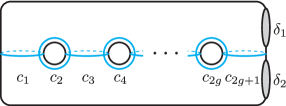
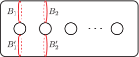
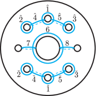
The odd chain relation in Mod(Σg2)ModsuperscriptsubscriptΣ𝑔2\operatorname{Mod}(\Sigma_{g}^{2}), with cisubscript𝑐𝑖c_{i} as in Figure 1(a)

(1) (tc1tc2tc2g+1)2g+2=tδ1tδ2,superscriptsubscript𝑡subscript𝑐1subscript𝑡subscript𝑐2subscript𝑡subscript𝑐2𝑔12𝑔2subscript𝑡subscript𝛿1subscript𝑡subscript𝛿2(t_{c_{1}}t_{c_{2}}\cdots t_{c_{2g+1}})^{2g+2}=t_{\delta_{1}}t_{\delta_{2}}\,,

is the monodromy factorization of a genus–g𝑔g pencil on a simply-connected Kähler surface, which is the K3K3{\rm K3} surface when g=2𝑔2g=2 [31]. Since the 2subscript2\mathbb{Z}_{2}–homology classes of c1,,c2g+1subscript𝑐1subscript𝑐2𝑔1c_{1},\ldots,c_{2g+1} generate H1(Σg2;2)subscript𝐻1superscriptsubscriptΣ𝑔2subscript2H_{1}(\Sigma_{g}^{2};\mathbb{Z}_{2}), and the sum of all odd indexed cisubscript𝑐𝑖c_{i} is homologous to each δjsubscript𝛿𝑗\delta_{j}, we see that there is in fact a unique quadratic form q:H1(Σg2;2)2:𝑞subscript𝐻1superscriptsubscriptΣ𝑔2subscript2subscript2q\colon H_{1}(\Sigma_{g}^{2};\mathbb{Z}_{2})\to\mathbb{Z}_{2} for which the monodromy curves satisfy the spin condition (corresponding to the unique spin structure on the 444–manifold) if and only if g𝑔g is even.

Example 5.

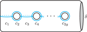
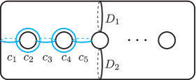
The even chain relation in Mod(Σg1)ModsuperscriptsubscriptΣ𝑔1\operatorname{Mod}(\Sigma_{g}^{1}), with cisubscript𝑐𝑖c_{i} as in Figure 1(b)

(2) (tc1tc2tc2g)4g+2=tδ,superscriptsubscript𝑡subscript𝑐1subscript𝑡subscript𝑐2subscript𝑡subscript𝑐2𝑔4𝑔2subscript𝑡𝛿(t_{c_{1}}t_{c_{2}}\cdots t_{c_{2g}})^{4g+2}=t_{\delta}\,,

is the monodromy factorization of a genus–g𝑔g pencil on a simply-connected Kähler surface. Since the 2subscript2\mathbb{Z}_{2}–homology classes of the curves c1,,c2gsubscript𝑐1subscript𝑐2𝑔c_{1},\ldots,c_{2g} generate H1(Σg1;2)subscript𝐻1superscriptsubscriptΣ𝑔1subscript2H_{1}(\Sigma_{g}^{1};\mathbb{Z}_{2}), there is in fact a unique quadratic form q:H1(Σg1;2)2:𝑞subscript𝐻1superscriptsubscriptΣ𝑔1subscript2subscript2q\colon H_{1}(\Sigma_{g}^{1};\mathbb{Z}_{2})\to\mathbb{Z}_{2} for which q(ci)=1𝑞subscript𝑐𝑖1q(c_{i})=1 for all i𝑖i. To check the remaining condition on the boundary components, take c2g+1subscript𝑐2𝑔1c_{2g+1} to be any curve extending the 2g2𝑔2g–chain c1,,c2gsubscript𝑐1subscript𝑐2𝑔c_{1},\ldots,c_{2g} to a (2g+1)2𝑔1(2g+1)–chain on Σg1superscriptsubscriptΣ𝑔1\Sigma_{g}^{1}. Now we see that all the odd indexed cisubscript𝑐𝑖c_{i} cobound a Σ0g+1superscriptsubscriptΣ0𝑔1\Sigma_{0}^{g+1}, and together with δ𝛿\delta, they also cobound a Σ0g+2superscriptsubscriptΣ0𝑔2\Sigma_{0}^{g+2}. So we have q(c2g+1)i=1gq(c2i1)𝑞subscript𝑐2𝑔1superscriptsubscript𝑖1𝑔𝑞subscript𝑐2𝑖1q(c_{2g+1})\equiv\sum_{i=1}^{g}q(c_{2i-1}) (mod 222), and q(δ)q(c2g+1)+i=1gq(c2i1)2q(c2g+1)0𝑞𝛿𝑞subscript𝑐2𝑔1superscriptsubscript𝑖1𝑔𝑞subscript𝑐2𝑖12𝑞subscript𝑐2𝑔10q(\delta)\equiv q(c_{2g+1})+\sum_{i=1}^{g}q(c_{2i-1})\equiv 2q(c_{2g+1})\equiv 0 (mod 222). Hence, these 444–manifolds are never spin.

Refer to caption
(a) Odd chain.
Refer to caption
(b) Even chain.
Refer to caption
(c) Hyperelliptic relation.
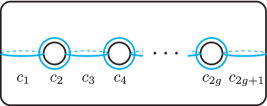
Figure 1. Dehn twist curves for standard relations.
Example 6.

The hyperelliptic relation in Mod(Σg)ModsubscriptΣ𝑔\operatorname{Mod}(\Sigma_{g}), with cisubscript𝑐𝑖c_{i} as in Figure 1(c)

(3) (tc1tc2tc2gtc2g+12tc2gtc2tc1)2=1,superscriptsubscript𝑡subscript𝑐1subscript𝑡subscript𝑐2subscript𝑡subscript𝑐2𝑔superscriptsubscript𝑡subscript𝑐2𝑔12subscript𝑡subscript𝑐2𝑔subscript𝑡subscript𝑐2subscript𝑡subscript𝑐121(t_{c_{1}}t_{c_{2}}\cdots t_{c_{2g}}t_{c_{2g+1}}^{2}t_{c_{2g}}\cdots t_{c_{2}}t_{c_{1}})^{2}=1\,,

is the monodromy factorization of a genus–g𝑔g fibration on the rational surface #2(4g+5)¯2{\mathbb{CP}}{}^{2}\#(4g+5)\overline{\mathbb{CP}}{}^{2}, and the double of this factorization is known to yield a genus–g𝑔g Lefschetz fibration on the elliptic surface E(g+1)𝐸𝑔1E(g+1) [31]. Once again, the 2subscript2\mathbb{Z}_{2}–homology classes of the curves c1,,c2g+1subscript𝑐1subscript𝑐2𝑔1c_{1},\ldots,c_{2g+1} generate H1(Σg;2)subscript𝐻1subscriptΣ𝑔subscript2H_{1}(\Sigma_{g};\mathbb{Z}_{2}), and because the odd indexed cisubscript𝑐𝑖c_{i} all together bound a subsurface, there is a unique quadratic form q:H1(Σg;2)2:𝑞subscript𝐻1subscriptΣ𝑔subscript2subscript2q\colon H_{1}(\Sigma_{g};\mathbb{Z}_{2})\to\mathbb{Z}_{2} for which q(ci)=1𝑞subscript𝑐𝑖1q(c_{i})=1 for all i𝑖i, if and only if g𝑔g is odd.

Yet, even when g𝑔g is odd, the total space #2(4g+5)¯2{\mathbb{CP}}{}^{2}\#(4g+5)\overline{\mathbb{CP}}{}^{2} for the positive factorization (3) is obviously not spin, despite the fiber class being primitive (which is immediate by the particular case of Proposition 8 below, or by the fibration admitting sections). Indeed, this fibration arises as a blow-up of a pencil on a Hirzebruch surface, and admits as many as 4g+44𝑔44g+4 exceptional sections, each one of which can be taken as the dual S𝑆S. As an instance of Proposition 3 however, when we double the monodromy factorization (3), we get a spin Lefschetz fibration, which yields the unique spin structure on E(g+1)𝐸𝑔1E(g+1), for g𝑔g odd. This is also evident from Theorem 2 and the fact that by matching the exceptional sections, we see that the latter fibration has a section S:=S#Sassignsuperscript𝑆𝑆#𝑆S^{\prime}:=S\#S with self-intersection 22-2. Similarly, if we cap off the two boundary components in Example 4, we get a positive factorization of the identity, and doubling it, we get a monodromy factorization for a spin Lefschetz fibration, provided g𝑔g is odd. Note that in both examples, we have the same spin structure on ΣgsubscriptΣ𝑔\Sigma_{g}, and the corresponding quadratic form has Arf invariant 111 when g1𝑔1g\equiv 1 (mod 4) and 00 when g3𝑔3g\equiv 3 (mod 4).

On the other hand, if we cap off the boundary component in Example 5, the monodromy curves, which are in this case linearly independent in homology, already satisfy the spin condition for any genus g𝑔g, and doubling it yields a spin Lefschetz fibration. The quadratic form for this unique spin structure on ΣgsubscriptΣ𝑔\Sigma_{g} now has Arf invariant 111 when g1𝑔1g\equiv 1 or 222 (mod 4) and 00 when g3𝑔3g\equiv 3 or 444 (mod 4).

Example 7.

A less known relation in Mod(Σg)ModsubscriptΣ𝑔\operatorname{Mod}(\Sigma_{g}) discovered by K.-H. Yun [63], which is a simultaneous generalization of the hyperelliptic relation and the Matsumoto-Cadavid-Korkmaz relation [42, 37] (all coming from different involutions), is as follows:

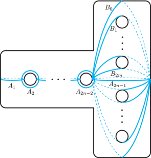
(4) (tA2n2tA2n3tA2tA12tA2tA2n3tA2n2tB0tB2mtA2n1)2=1,superscriptsubscript𝑡subscript𝐴2𝑛2subscript𝑡subscript𝐴2𝑛3subscript𝑡subscript𝐴2superscriptsubscript𝑡subscript𝐴12subscript𝑡subscript𝐴2subscript𝑡subscript𝐴2𝑛3subscript𝑡subscript𝐴2𝑛2subscript𝑡subscript𝐵0subscript𝑡subscript𝐵2𝑚subscript𝑡subscript𝐴2𝑛121(t_{A_{2n-2}}t_{A_{2n-3}}\cdots t_{A_{2}}t_{A_{1}}^{2}t_{A_{2}}\cdots t_{A_{2n-3}}t_{A_{2n-2}}\,t_{B_{0}}\cdots t_{B_{2m}}t_{A_{2n-1}})^{2}=1\,,

where Ai,Bjsubscript𝐴𝑖subscript𝐵𝑗A_{i},B_{j} are as in Figure 2, and m,n>0𝑚𝑛0m,n>0. This is the monodromy factorization of a genus g=2m+n1𝑔2𝑚𝑛1g=2m+n-1 fibration on the ruled surface (Σm×S2)# 4n¯2(\Sigma_{m}\times S^{2})\,\#\,4n\overline{\mathbb{CP}}{}^{2}, and importantly, a twisted fiber sum of two copies of this fibration is known to yield a genus–g𝑔g Lefschetz fibration with several (2(-2)–sections, the total space of which is a knot surgered elliptic surface E(n)K𝐸subscript𝑛𝐾E(n)_{K}, where K𝐾K is a fibered knot of genus m𝑚m [27, 63]. Since E(n)K𝐸subscript𝑛𝐾E(n)_{K} are homeomorphic to E(n)𝐸𝑛E(n) [26], in particular we deduce that there is a twisted fiber sum of two copies of this fibration that is simply-connected, and moreover spin with signature 8n8𝑛-8n when n𝑛n is even.

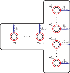
Let {αi,βi}i=1n1{αj,βj}j=12msuperscriptsubscriptsubscript𝛼𝑖subscript𝛽𝑖𝑖1𝑛1superscriptsubscriptsubscriptsuperscript𝛼𝑗subscriptsuperscript𝛽𝑗𝑗12𝑚\{\alpha_{i},\beta_{i}\}_{i=1}^{n-1}\cup\{\alpha^{\prime}_{j},\beta^{\prime}_{j}\}_{j=1}^{2m} be a symplectic basis of H1(Σg;2)subscript𝐻1subscriptΣ𝑔subscript2H_{1}(\Sigma_{g};\mathbb{Z}_{2}), represented by the same labeled curves in Figure 2. We calculate the 2subscript2\mathbb{Z}_{2}–homology classes of the vanishing cycles as

A1subscript𝐴1\displaystyle A_{1} =β1,absentsubscript𝛽1\displaystyle=\beta_{1},
A2i1subscript𝐴2𝑖1\displaystyle A_{2i-1} =βi1+βi(i=2,,n1),absentsubscript𝛽𝑖1subscript𝛽𝑖𝑖2𝑛1\displaystyle=\beta_{i-1}+\beta_{i}\quad(i=2,\ldots,n-1),
A2n1subscript𝐴2𝑛1\displaystyle A_{2n-1} =βn1,absentsubscript𝛽𝑛1\displaystyle=\beta_{n-1},
A2isubscript𝐴2𝑖\displaystyle A_{2i} =αi(i=1,,n1),absentsubscript𝛼𝑖𝑖1𝑛1\displaystyle=\alpha_{i}\quad(i=1,\ldots,n-1),
B0subscript𝐵0\displaystyle B_{0} =α1++α2m+βn1,absentsuperscriptsubscript𝛼1superscriptsubscript𝛼2𝑚subscript𝛽𝑛1\displaystyle=\alpha_{1}^{\prime}+\cdots+\alpha_{2m}^{\prime}+\beta_{n-1},
B2jsubscript𝐵2𝑗\displaystyle B_{2j} =αj+1++α2mj+βj+β2m+1j+βn1(j=1,,m1),absentsuperscriptsubscript𝛼𝑗1superscriptsubscript𝛼2𝑚𝑗superscriptsubscript𝛽𝑗superscriptsubscript𝛽2𝑚1𝑗subscript𝛽𝑛1𝑗1𝑚1\displaystyle=\alpha_{j+1}^{\prime}+\cdots+\alpha_{2m-j}^{\prime}+\beta_{j}^{\prime}+\beta_{2m+1-j}^{\prime}+\beta_{n-1}\quad(j=1,\ldots,m-1),
B2msubscript𝐵2𝑚\displaystyle B_{2m} =βm+βm+1+βn1,absentsuperscriptsubscript𝛽𝑚superscriptsubscript𝛽𝑚1subscript𝛽𝑛1\displaystyle=\beta_{m}^{\prime}+\beta_{m+1}^{\prime}+\beta_{n-1},
B2j1subscript𝐵2𝑗1\displaystyle B_{2j-1} =αj++α2m+1j+βj+β2m+1j+βn1(j=1,,m).absentsuperscriptsubscript𝛼𝑗superscriptsubscript𝛼2𝑚1𝑗superscriptsubscript𝛽𝑗superscriptsubscript𝛽2𝑚1𝑗subscript𝛽𝑛1𝑗1𝑚\displaystyle=\alpha_{j}^{\prime}+\cdots+\alpha_{2m+1-j}^{\prime}+\beta_{j}^{\prime}+\beta_{2m+1-j}^{\prime}+\beta_{n-1}\quad(j=1,\ldots,m).

If n𝑛n is odd then no quadratic form q:H1(Σg;2)2:𝑞subscript𝐻1subscriptΣ𝑔subscript2subscript2q\colon H_{1}(\Sigma_{g};\mathbb{Z}_{2})\to\mathbb{Z}_{2} satisfies q(Ai)=1𝑞subscript𝐴𝑖1q(A_{i})=1 for all odd i𝑖i since such Aisubscript𝐴𝑖A_{i} cobound a subsurface ΣmnsuperscriptsubscriptΣ𝑚𝑛\Sigma_{m}^{n}. Suppose that n𝑛n is even. Let q(αi)=q(αj)=q(βj)=1𝑞subscript𝛼𝑖𝑞subscriptsuperscript𝛼𝑗𝑞subscriptsuperscript𝛽𝑗1q(\alpha_{i})=q(\alpha^{\prime}_{j})=q(\beta^{\prime}_{j})=1 for all i,j𝑖𝑗i,j, and set q(βi)=1𝑞subscript𝛽𝑖1q(\beta_{i})=1 for all odd 1in11𝑖𝑛11\leq i\leq n-1 and q(βi)=0𝑞subscript𝛽𝑖0q(\beta_{i})=0 for all even 2in22𝑖𝑛22\leq i\leq n-2. This defines a quadratic form on H1(Σg;2)subscript𝐻1subscriptΣ𝑔subscript2H_{1}(\Sigma_{g};\mathbb{Z}_{2}) for which q(Ai)=q(Bj)=1𝑞subscript𝐴𝑖𝑞subscript𝐵𝑗1q(A_{i})=q(B_{j})=1 for all i,j𝑖𝑗i,j, and the Arf invariant of this quadratic form is 00 when n0𝑛0n\equiv 0 (mod 4) and 111 when n2𝑛2n\equiv 2 (mod 4).

Refer to caption
Refer to caption
Figure 2. Dehn twist curves of Yun’s relation and the homology generators.

We will next show, when there is no information available for a section, how, using the monodromy, we can still determine whether the fiber is primitive and thus has an algebraic dual as required in Theorem 2. Since the kernel of the forgetful homomorphism Mod(Σg,1)Mod(Σg)ModsubscriptΣ𝑔1ModsubscriptΣ𝑔\operatorname{Mod}(\Sigma_{g,1})\to\operatorname{Mod}(\Sigma_{g}) is generated by point-pushing maps [22], if we take an arbitrary marked point on ΣgsubscriptΣ𝑔\Sigma_{g} avoiding all the cisubscript𝑐𝑖c_{i}, we still get a lift   tc1tcn=𝒫α1𝒫αmsubscript𝑡subscriptsuperscript𝑐1subscript𝑡subscriptsuperscript𝑐𝑛subscript𝒫subscript𝛼1subscript𝒫subscript𝛼𝑚t_{c^{\prime}_{1}}\cdots t_{c^{\prime}_{n}}=\mathcal{P}_{\vec{\alpha}_{1}}\cdots\mathcal{P}_{\vec{\alpha}_{m}}\, in Mod(Σg,1)ModsubscriptΣ𝑔1\operatorname{Mod}(\Sigma_{g,1}), where on the right-hand side we now have point-pushing maps along oriented loops αisubscript𝛼𝑖\vec{\alpha}_{i}. This product of point-pushing maps can be expressed as one point-pushing map along a possibly immersed oriented loop α𝛼\vec{\alpha}, and when α𝛼\alpha is null-homotopic, the marked point we picked in fact gives an honest section of the fibration.

Proposition 8.

Let (X,f)𝑋𝑓(X,f) be a genus–g𝑔g Lefschetz fibration, which has a monodromy factorization tc1tcn=1subscript𝑡subscript𝑐1subscript𝑡subscript𝑐𝑛1t_{c_{1}}\cdots t_{c_{n}}=1, with the following lift in Mod(Σg,1)ModsubscriptΣ𝑔1\operatorname{Mod}(\Sigma_{g,1}):

tc1tcn=𝒫α1𝒫αm.subscript𝑡subscriptsuperscript𝑐1subscript𝑡subscriptsuperscript𝑐𝑛subscript𝒫subscript𝛼1subscript𝒫subscript𝛼𝑚t_{c^{\prime}_{1}}\cdots t_{c^{\prime}_{n}}=\mathcal{P}_{\vec{\alpha}_{1}}\cdots\mathcal{P}_{\vec{\alpha}_{m}}\,.

Let γisubscript𝛾𝑖\gamma_{i} be the homology class of cisubscript𝑐𝑖c_{i} taken with either orientation for i=1,,n𝑖1𝑛i=1,\ldots,n, and let α𝛼\alpha be the sum of the homology classes of all αjsubscript𝛼𝑗\vec{\alpha}_{j} in H1(Σg)subscript𝐻1subscriptΣ𝑔H_{1}(\Sigma_{g}). The divisibility of the homology class of the regular fiber F𝐹F in H2(X)subscript𝐻2𝑋H_{2}(X) is the smallest positive integer d𝑑d such that the image of dα𝑑𝛼d\alpha under the homomorphism H1(Σg)H1(Σg)/γ1,,γnsubscript𝐻1subscriptΣ𝑔subscript𝐻1subscriptΣ𝑔subscript𝛾1subscript𝛾𝑛H_{1}(\Sigma_{g})\to H_{1}(\Sigma_{g})\,/\langle\gamma_{1},\ldots,\gamma_{n}\rangle is trivial. In particular, if {γi}i=1nsuperscriptsubscriptsubscript𝛾𝑖𝑖1𝑛\{\gamma_{i}\}_{i=1}^{n} generate H1(Σg)subscript𝐻1subscriptΣ𝑔H_{1}(\Sigma_{g}), then [F]delimited-[]𝐹[F] is primitive.

Proof.

We have X=X(D2×Σg)𝑋superscript𝑋superscript𝐷2subscriptΣ𝑔X=X^{\prime}\cup(D^{2}\times\Sigma_{g}), where X=(D2×Σg)i=1nhisuperscript𝑋superscript𝐷2subscriptΣ𝑔superscriptsubscript𝑖1𝑛subscript𝑖X^{\prime}=(D^{2}\times\Sigma_{g})\cup\,\sum_{i=1}^{n}h_{i} and {hi}subscript𝑖\{h_{i}\} are the Lefschetz 222–handles attached along cisubscript𝑐𝑖c_{i} on ΣgsubscriptΣ𝑔\Sigma_{g}. So Xsuperscript𝑋X^{\prime} contains all the 222–handles of X𝑋X but one, which comes from the second copy of D2×Σgsuperscript𝐷2subscriptΣ𝑔D^{2}\times\Sigma_{g} in the decomposition of X𝑋X. The isotopy, which takes the product tc1tcnsubscript𝑡subscript𝑐1subscript𝑡subscript𝑐𝑛t_{c_{1}}\cdots t_{c_{n}} to 111 in Diff+(Σg)superscriptDiffsubscriptΣ𝑔\mathrm{Diff}^{+}(\Sigma_{g}), prescribes a fiber–preserving diffeomorphism ΦΦ\Phi from the boundary fibration f|Xevaluated-at𝑓superscript𝑋f|_{\partial X^{\prime}} to the trivial ΣgsubscriptΣ𝑔\Sigma_{g}–fibration on D2×Σgsuperscript𝐷2subscriptΣ𝑔\partial D^{2}\times\Sigma_{g}. The attaching circle csuperscript𝑐c^{\prime} of the last 222–handle hsuperscripth^{\prime} is a section s:=Φ1(D2×p)assignsuperscript𝑠superscriptΦ1superscript𝐷2𝑝s^{\prime}:=\Phi^{-1}(\partial D^{2}\times p) of f|Xevaluated-at𝑓superscript𝑋f|_{\partial X^{\prime}}, for some point pΣg𝑝subscriptΣ𝑔p\in\Sigma_{g}.

In the standard handle diagram of Xsuperscript𝑋X^{\prime}, the attaching circle csuperscript𝑐c^{\prime} of hsuperscripth^{\prime} links the 222–handle of the fiber geometrically once, and possibly goes over the 111–handles coming from ΣgsubscriptΣ𝑔\Sigma_{g}, and links with the attaching circles {ci}subscript𝑐𝑖\{c_{i}\} of the Lefschetz 222–handles {hi}subscript𝑖\{h_{i}\}. While the section ssuperscript𝑠s^{\prime} of f|Xevaluated-at𝑓superscript𝑋f|_{\partial X^{\prime}} carries the first information, i.e. how csuperscript𝑐c^{\prime} would go over the 111–handles as it traverses around D2×psuperscript𝐷2𝑝\partial D^{2}\times p once, there are still many ways hsuperscripth^{\prime} can be attached along a circle c𝑐c in the complement of the attaching circles {ci}subscript𝑐𝑖\{c_{i}\} —where c𝑐c, even if it is not isotopic to csuperscript𝑐c^{\prime} in the diagram, is still isotopic to ssuperscript𝑠s^{\prime} on Xsuperscript𝑋{\partial X^{\prime}}. Equivalently, there are several ways to isotope all the attaching circles {ci}subscript𝑐𝑖\{c_{i}\} in the diagram to curves that will project on to ΣgsubscriptΣ𝑔\Sigma_{g} still as embedded curves {ci}subscriptsuperscript𝑐𝑖\{c^{\prime}_{i}\}, while now avoiding a marked point corresponding to c𝑐c. Each one of them prescribes a lift of the identity tc1tcn=1subscript𝑡subscript𝑐1subscript𝑡subscript𝑐𝑛1t_{c_{1}}\cdots t_{c_{n}}=1 in Mod(Σg)ModsubscriptΣ𝑔\operatorname{Mod}(\Sigma_{g}) to a factorization tc1tcn=𝒫αsubscript𝑡subscriptsuperscript𝑐1subscript𝑡subscriptsuperscript𝑐𝑛subscript𝒫𝛼t_{c^{\prime}_{1}}\cdots t_{c^{\prime}_{n}}=\mathcal{P}_{\vec{\alpha}} in Mod(Σg,1)ModsubscriptΣ𝑔1\operatorname{Mod}(\Sigma_{g,1}), where α𝛼\vec{\alpha} is an oriented curve on ΣgsubscriptΣ𝑔\Sigma_{g}. However, c𝑐c and csuperscript𝑐c^{\prime} only differ by handle slides over hisubscript𝑖h_{i}, and the homology classes of their attaching circles on ΣgsubscriptΣ𝑔\Sigma_{g} will only differ by relations generated by the homology classes of {ci}subscript𝑐𝑖\{c_{i}\} in H1(Σg)subscript𝐻1subscriptΣ𝑔H_{1}(\Sigma_{g}). Thus, they will all map to the same homology class under the projection H1(Σg)H1(Σg)/γ1,,γnsubscript𝐻1subscriptΣ𝑔subscript𝐻1subscriptΣ𝑔subscript𝛾1subscript𝛾𝑛H_{1}(\Sigma_{g})\to H_{1}(\Sigma_{g})\,/\langle\gamma_{1},\ldots,\gamma_{n}\rangle.

Corresponding to a given lift tc1tcn=𝒫α1𝒫αmsubscript𝑡subscriptsuperscript𝑐1subscript𝑡subscriptsuperscript𝑐𝑛subscript𝒫subscript𝛼1subscript𝒫subscript𝛼𝑚t_{c^{\prime}_{1}}\cdots t_{c^{\prime}_{n}}=\mathcal{P}_{\vec{\alpha}_{1}}\cdots\mathcal{P}_{\vec{\alpha}_{m}} in Mod(Σg,1)ModsubscriptΣ𝑔1\operatorname{Mod}(\Sigma_{g,1}) is such a choice c𝑐c as above. To see this, let π:S1×ΣgΣg:𝜋superscript𝑆1subscriptΣ𝑔subscriptΣ𝑔\pi\colon S^{1}\times\Sigma_{g}\to\Sigma_{g} be the projection, and let t𝑡t parametrize S1=[0,1]/0 1superscript𝑆1010similar-to1S^{1}=[0,1]\,/0\,{\small\sim}\,1. Take a partition 0=t0<t1<<ti<<tm=10subscript𝑡0subscript𝑡1subscript𝑡𝑖subscript𝑡𝑚10=t_{0}<t_{1}<\ldots<t_{i}<\ldots<t_{m}=1. For each αisubscript𝛼𝑖\vec{\alpha}_{i}, we can find an oriented arc βisubscript𝛽𝑖\beta_{i} in [ti1,ti]×Σgt_{i-1},t_{i}]\times\Sigma_{g}, running from the point ti1×psubscript𝑡𝑖1𝑝t_{i-1}\times p to the point ti×psubscript𝑡𝑖𝑝t_{i}\times p, so that the π|βi:βiαi:evaluated-at𝜋subscript𝛽𝑖subscript𝛽𝑖subscript𝛼𝑖\pi|_{\beta_{i}}\colon\beta_{i}\to\vec{\alpha}_{i} is an immersion. Concatenating all of them, we get an oriented arc β𝛽\beta in [0,1]×Σg01subscriptΣ𝑔[0,1]\times\Sigma_{g}. Identifying the end points of either +β𝛽+\beta or β𝛽-\beta, we obtain c𝑐c. Just like our reading of the self-intersection number of a section from the corresponding monodromy factorization, the correct sign of β𝛽\beta here can be settled for once and all after calculating it in one example, but for our homology calculations to follow, the sign will not matter.

From the decomposition X=X(D2×Σg)𝑋superscript𝑋superscript𝐷2subscriptΣ𝑔X=X^{\prime}\,\cup\,(D^{2}\times\Sigma_{g}), it is clear that there is no class with a representative in Xsuperscript𝑋X^{\prime} which has non-trivial pairing with the homology class of the regular fiber F𝐹F in H2(X)subscript𝐻2𝑋H_{2}(X). By our discussion above, up to relations generated by the homology classes γisubscript𝛾𝑖\gamma_{i} of cisubscript𝑐𝑖c_{i} on H1(Σg)subscript𝐻1subscriptΣ𝑔H_{1}(\Sigma_{g}), the attaching circle csuperscript𝑐c^{\prime} of the last 222–handle hsuperscripth^{\prime} is homologous to c𝑐c we build from a given lift, which in turn is homologous to a concatenation of S1×psuperscript𝑆1𝑝S^{1}\times p and all αjsubscript𝛼𝑗\vec{\alpha}_{j}s in H1(S1×Σg)=H1(S1)×H1(Σg)subscript𝐻1superscript𝑆1subscriptΣ𝑔subscript𝐻1superscript𝑆1subscript𝐻1subscriptΣ𝑔H_{1}(S^{1}\times\Sigma_{g})=H_{1}(S^{1})\times H_{1}(\Sigma_{g}). Since the S1×psuperscript𝑆1𝑝S^{1}\times p curve already bounds D2×psuperscript𝐷2𝑝D^{2}\times p, when we attach hsuperscripth^{\prime}, its attaching circle becomes homologous to ±αplus-or-minus𝛼\pm\alpha in H1(S1×Σg)subscript𝐻1superscript𝑆1subscriptΣ𝑔H_{1}(S^{1}\times\Sigma_{g}), for α=j=1m[αj]𝛼superscriptsubscript𝑗1𝑚delimited-[]subscript𝛼𝑗\alpha=\sum_{j=1}^{m}[\vec{\alpha}_{j}] in H1(Σg)subscript𝐻1subscriptΣ𝑔H_{1}(\Sigma_{g}). It follows that if the image of α𝛼\alpha is trivial in the quotient H1(Σg)/γ1,,γnH1(X)subscript𝐻1subscriptΣ𝑔subscript𝛾1subscript𝛾𝑛subscript𝐻1superscript𝑋H_{1}(\Sigma_{g})\,/\langle\gamma_{1},\ldots,\gamma_{n}\rangle\cong H_{1}(X^{\prime}), then the attaching circle of hsuperscripth^{\prime} bounds some surface Ssuperscript𝑆S^{\prime} in Xsuperscript𝑋X^{\prime}. We can then form a closed surface S𝑆S in X𝑋X by gluing Ssuperscript𝑆S^{\prime} and the core of hsuperscripth^{\prime} to obtain a surface which intersects the fiber F𝐹F once, and conclude that [F]delimited-[]𝐹[F] is primitive.

In general, if the image of dα𝑑𝛼d\,\alpha is trivial in H1(Σg)/γ1,,γnsubscript𝐻1subscriptΣ𝑔subscript𝛾1subscript𝛾𝑛H_{1}(\Sigma_{g})\,/\langle\gamma_{1},\ldots,\gamma_{n}\rangle, we get a surface Ssuperscript𝑆S^{\prime} in Xsuperscript𝑋X^{\prime} that bounds d𝑑d parallel copies of the attaching circle of hsuperscripth^{\prime}. So we can build a closed surface S𝑆S in X𝑋X, which satisfies SF=d𝑆𝐹𝑑S\cdot F=d, by gluing Ssuperscript𝑆S^{\prime} and d𝑑d parallel copies of the core of the 222–handle hsuperscripth^{\prime}. Conversely, if [F]=dF0delimited-[]𝐹𝑑subscript𝐹0[F]=dF_{0} for a primitive class F0subscript𝐹0F_{0}, let S𝑆S be a surface in X𝑋X representing the dual of F0subscript𝐹0F_{0}, so SF=d𝑆𝐹𝑑S\cdot F=d. If necessary, by tubing —along F𝐹F— between any pair of positive and negative intersections of S𝑆S with F𝐹F, we can replace S𝑆S with a higher genus surface in the same homology class, which now intersects F𝐹F geometrically d𝑑d times. We can then isotope this S𝑆S so that in a small neighborhood N(F)𝑁𝐹N(F) of F𝐹F identified as N(F)D2×Σg𝑁𝐹superscript𝐷2subscriptΣ𝑔N(F)\cong D^{2}\times\Sigma_{g}, we have SN(F)D2×d points𝑆𝑁𝐹superscript𝐷2𝑑 pointsS\cap N(F)\cong D^{2}\times d\textrm{ points}. Identifying N(F)𝑁𝐹N(F) with D2×Σgsuperscript𝐷2subscriptΣ𝑔D^{2}\times\Sigma_{g} in the decomposition X=X(D2×Σg)𝑋superscript𝑋superscript𝐷2subscriptΣ𝑔X=X^{\prime}\cup\,(D^{2}\times\Sigma_{g}), we conclude that any class dual to the primitive root F0subscript𝐹0F_{0} of [F]delimited-[]𝐹[F] can in fact be represented by a surface S𝑆S that splits into a surface Ssuperscript𝑆S^{\prime} in Xsuperscript𝑋X^{\prime} and d𝑑d parallel copies of the core of hsuperscripth^{\prime}. Hence, the smallest positive integer d𝑑d, for which dα𝑑𝛼d\,\alpha is trivial in the quotient, gives the divisibility of the fiber class [F]delimited-[]𝐹[F] in H2(X)subscript𝐻2𝑋H_{2}(X). ∎

In the case of pencils, the induced handle decomposition nullifies the need for the additional information on the attaching of the last 222–handle, and one can determine the divisibility of the fiber class of a genus–g𝑔g Lefschetz pencil with b𝑏b base points directly using a lift of the monodromy in Mod(Σgb)ModsuperscriptsubscriptΣ𝑔𝑏\operatorname{Mod}(\Sigma_{g}^{b}); see [33, Appendix].

We will call a surface S𝑆S a pseudosection of (X,f)𝑋𝑓(X,f) if it intersects a regular fiber F𝐹F once. As seen from our proof of Proposition 8, when the lift of the monodromy factorization to Mod(Σg,1)ModsubscriptΣ𝑔1\operatorname{Mod}(\Sigma_{g,1}) involves non-trivial point-pushing maps, one gets a pseudosection (possibly after some handle slides over the Lefschetz 222–handles), provided the class α𝛼\alpha determined by the point-pushing curves becomes trivial under the quotient homomorphism H1(Σg)H1(Σg)/γ1,,γnsubscript𝐻1subscriptΣ𝑔subscript𝐻1subscriptΣ𝑔subscript𝛾1subscript𝛾𝑛H_{1}(\Sigma_{g})\to H_{1}(\Sigma_{g})\,/\langle\gamma_{1},\ldots,\gamma_{n}\rangle, and conversely any pseudosection yields such a lift. However, unlike in the case of a section, now a further lift to Mod(Σg1)ModsuperscriptsubscriptΣ𝑔1\operatorname{Mod}(\Sigma_{g}^{1}) does not allow us to directly determine the self-intersection number of S𝑆S.111In principle, one can of course attempt to access all this information by first drawing the standard handle diagram for (X,f|X)superscript𝑋evaluated-at𝑓superscript𝑋(X^{\prime},f|_{X^{\prime}}) , then finding a sequence of Kirby moves from the induced diagram on Xsuperscript𝑋\partial X^{\prime} to the standard handle diagram of S1×Σgsuperscript𝑆1subscriptΣ𝑔S^{1}\times\Sigma_{g} with 2g2𝑔2g 111–handles and a 222–handle, and finally dragging back a 00–framed meridian to the 222–handle in the latter diagram to a 222–handle in the former, so as to calculate its framing, and so on. However, this not only proves to be a difficult exercise even for Kirby calculus aficionados, but also departs from our general approach to read off all the essential information from monodromy factorizations.

We will show that, under favorable conditions that apply to all the examples we will deal with in this article, knowing that the fiber class is primitive will be enough to build the spin structure:

Theorem 9.

Let (X,f)𝑋𝑓(X,f) be a genus–g𝑔g Lefschetz fibration with a monodromy factorization tc1tcn=1subscript𝑡subscript𝑐1subscript𝑡subscript𝑐𝑛1t_{c_{1}}\cdots t_{c_{n}}=1, a primitive fiber class in H2(X)subscript𝐻2𝑋H_{2}(X), and signature σ(X)0𝜎𝑋0\sigma(X)\equiv 0 (mod 16). Assume that there is a quadratic form q:H1(Σg;2)2:𝑞subscript𝐻1subscriptΣ𝑔subscript2subscript2q\colon H_{1}(\Sigma_{g};\mathbb{Z}_{2})\to\mathbb{Z}_{2} with respect to the 2subscript2\mathbb{Z}_{2}–intersection pairing, such that q(ci)=1𝑞subscript𝑐𝑖1q(c_{i})=1 for all i𝑖i, and Arf(q)=1Arf𝑞1\textrm{Arf}\,(q)=1. Then any spin structure ssuperscript𝑠s^{\prime} corresponding to a quadratic form qsuperscript𝑞q^{\prime} on H1(Σg;2)subscript𝐻1subscriptΣ𝑔subscript2H_{1}(\Sigma_{g};\mathbb{Z}_{2}) with q(ci)=1superscript𝑞subscript𝑐𝑖1q^{\prime}(c_{i})=1 for all i𝑖i, induces a spin structure on X𝑋X.

Proof.

Let us first assume that there exists a genus–g𝑔g achiral Lefschetz fibration (Yg,fg)subscript𝑌𝑔subscript𝑓𝑔(Y_{g},f_{g}), with a monodromy factorization td1ϵ1tdmϵm=1superscriptsubscript𝑡subscript𝑑1subscriptitalic-ϵ1superscriptsubscript𝑡subscript𝑑𝑚subscriptitalic-ϵ𝑚1t_{d_{1}}^{\epsilon_{1}}\cdots t_{d_{m}}^{\epsilon_{m}}=1 in Mod(Σg)ModsubscriptΣ𝑔\operatorname{Mod}(\Sigma_{g}) (for some ϵi=±1subscriptitalic-ϵ𝑖plus-or-minus1\epsilon_{i}=\pm 1), which satisfies the following four properties:

  1. (i)

    σ(Yg)8𝜎subscript𝑌𝑔8\sigma(Y_{g})\equiv 8 (mod 161616),

  2. (ii)

    fgsubscript𝑓𝑔f_{g} admits a section Sgsubscript𝑆𝑔S_{g} of (possibly positive) odd self-intersection,

  3. (iii)

    there is an sgSpin(Σg)subscript𝑠𝑔SpinsubscriptΣ𝑔s_{g}\in\mathrm{Spin}(\Sigma_{g}), with a quadratic form qgsubscript𝑞𝑔q_{g} such that qg(di)=1subscript𝑞𝑔subscript𝑑𝑖1q_{g}(d_{i})=1 for all i𝑖i,

  4. (iv)

    Arf(qg)=1Arfsubscript𝑞𝑔1\textrm{Arf}(q_{g})=1.

We will show in a bit that there are such model fibrations for every genus g1𝑔1g\geq 1.

Since (X,f)𝑋𝑓(X,f) has a primitive fiber class, by our discussion above, it has a pseudosection S𝑆S intersecting a regular fiber F𝐹F geometrically once. Let sSpin(Σg)𝑠SpinsubscriptΣ𝑔s\in\mathrm{Spin}(\Sigma_{g}) correspond to the quadratic form q𝑞q in the hypothesis.

Removing a small neighborhood N(F)𝑁𝐹N(F) of F𝐹F, where S𝑆S intersects F𝐹F once, and N(Fg)𝑁subscript𝐹𝑔N(F_{g}) of the regular fiber Fgsubscript𝐹𝑔F_{g} of (Yg,fg)subscript𝑌𝑔subscript𝑓𝑔(Y_{g},f_{g}), we can take a fiber sum (X^,f^)=(X,f)#(Yg,fg)^𝑋^𝑓𝑋𝑓#subscript𝑌𝑔subscript𝑓𝑔(\hat{X},\hat{f})=(X,f)\#(Y_{g},f_{g}), so that under the gluing (XN(F))(YN(Fg))𝑋𝑁𝐹𝑌𝑁subscript𝐹𝑔\partial(X\setminus N(F))\to\partial(Y\setminus N(F_{g})) we have SN(F)𝑆𝑁𝐹S\cap\,\partial N(F) sent to SgN(Fg)subscript𝑆𝑔𝑁subscript𝐹𝑔S_{g}\cap\,\partial N(F_{g}), which we can always achieve after an isotopy for any given fiber-preserving diffeomorphism. So this fibration has a pseudosection S^=(SSN(F))(SgSgN(Fg))=S#Sg^𝑆𝑆𝑆𝑁𝐹subscript𝑆𝑔subscript𝑆𝑔𝑁subscript𝐹𝑔𝑆#subscript𝑆𝑔\hat{S}=(S\setminus S\cap N(F))\cup(S_{g}\setminus S_{g}\cap N(F_{g}))=S\#S_{g}, with self-intersection S^S^=SS+SgSgSS+1^𝑆^𝑆𝑆𝑆subscript𝑆𝑔subscript𝑆𝑔𝑆𝑆1\hat{S}\cdot\hat{S}=S\cdot S+S_{g}\cdot S_{g}\equiv S\cdot S+1 (mod 222), as we assumed Sgsubscript𝑆𝑔S_{g} has odd self-intersection.

Identifying the boundaries N(F)𝑁𝐹\partial N(F) and N(Fg)𝑁subscript𝐹𝑔\partial N(F_{g}) with S1×Σgsuperscript𝑆1subscriptΣ𝑔S^{1}\times\Sigma_{g}, the gluing diffeomorphism is prescribed by a self-diffeomorphism ΦΦ\Phi of S1×Σgsuperscript𝑆1subscriptΣ𝑔S^{1}\times\Sigma_{g}, which is the product of the complex conjugation of the unit circle S1superscript𝑆1S^{1}\subset\mathbb{C}, and some ϕDiff+(Σg)italic-ϕsuperscriptDiffsubscriptΣ𝑔\phi\in\textrm{Diff}^{+}(\Sigma_{g}). Since both spin structures s𝑠s and sgsubscript𝑠𝑔s_{g} have the same Arf invariant, we can choose ϕitalic-ϕ\phi to be a spin diffeomorphism ϕ:(Σg,s)(Σg,sg):italic-ϕsubscriptΣ𝑔𝑠subscriptΣ𝑔subscript𝑠𝑔\phi\colon(\Sigma_{g},s)\to(\Sigma_{g},s_{g}). Now, the fibration (X^,f^)^𝑋^𝑓(\hat{X},\hat{f}) has monodromy curves {ci,ϕ1(dj)}subscript𝑐𝑖superscriptitalic-ϕ1subscript𝑑𝑗\{c_{i},\phi^{-1}(d_{j})\}, with q(ci)=1𝑞subscript𝑐𝑖1q(c_{i})=1 and q(ϕ1(dj))=qg(dj)=1𝑞superscriptitalic-ϕ1subscript𝑑𝑗subscript𝑞𝑔subscript𝑑𝑗1q(\phi^{-1}(d_{j}))=q_{g}(d_{j})=1 for all i,j𝑖𝑗i,j. If the pseudosection S𝑆S of (X,f)𝑋𝑓(X,f) had odd self-intersection, then S^^𝑆\hat{S} would have even self-intersection, and by Theorem 2, X^^𝑋\hat{X} would be spin. However, by Novikov additivity, the signature σ(X^)=σ(X)+σ(Yg)8𝜎^𝑋𝜎𝑋𝜎subscript𝑌𝑔8\sigma(\hat{X})=\sigma(X)+\sigma(Y_{g})\equiv 8 (mod 161616), and Rokhlin’s theorem implies that X^^𝑋\hat{X} cannot be spin. So we deduce that S𝑆S has even self-intersection, and thus we can invoke Theorem 2 to conclude that our original Lefschetz fibration (X,f)𝑋𝑓(X,f) is spin, in fact not only for q𝑞q, but for any quadratic form qsuperscript𝑞q^{\prime} with q(ci)=1superscript𝑞subscript𝑐𝑖1q^{\prime}(c_{i})=1 for all i𝑖i.

We are left with building the models (Yg,fg)subscript𝑌𝑔subscript𝑓𝑔(Y_{g},f_{g}). Note that by Proposition 3, any achiral Lefschetz fibration satisfying (iii) should necessarily have signature σ(Yg)0𝜎subscript𝑌𝑔0\sigma(Y_{g})\equiv 0 (mod 8). Some of these models can be derived immediately from Examples 46. When we cap off the boundary components, all these relations yield hyperelliptic Lefschetz fibrations, so using Endo’s signature formula for hyperelliptic fibrations [20], we can easily see that the even-chain relation yields Lefschetz fibrations with the desired properties when g2𝑔2g\equiv 2 (mod 4), whereas all three relations yield such examples when g1𝑔1g\equiv 1 (mod 4).

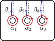
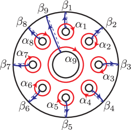
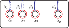
To get models for all g𝑔g however, we will go about it a little differently, and build achiral fibrations out of the smallest chain relations instead —while remembering that everything we have discussed so far also applies to achiral fibrations. Below, let {αi,βi}subscript𝛼𝑖subscript𝛽𝑖\{\alpha_{i},\beta_{i}\} be a symplectic basis for H1(Σg;2)subscript𝐻1subscriptΣ𝑔subscript2H_{1}(\Sigma_{g};\mathbb{Z}_{2}) generated by the same labeled curves given in Figure 3.
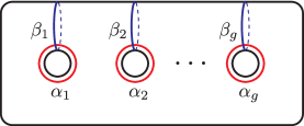
Refer to caption
Figure 3. The symplectic basis for H1(Σg;2)subscript𝐻1subscriptΣ𝑔subscript2H_{1}(\Sigma_{g};\mathbb{Z}_{2}).

g=1𝑔1g=1: Capped off even chain, odd chain and hyperelliptic relations all give Hurwitz equivalent positive factorizations, the monodromy curves of which evaluate as 111 under the quadratic form prescribed by q1(α1)=q1(β1)=1subscript𝑞1subscript𝛼1subscript𝑞1subscript𝛽11q_{1}(\alpha_{1})=q_{1}(\beta_{1})=1. Its signature is 88-8.

g=2𝑔2g=2: Capped off even chain relation gives a positive factorization, the monodromy curves of which evaluate as 111 under the quadratic form prescribed by q2(α1)=q2(β1)=q2(α2)=1subscript𝑞2subscript𝛼1subscript𝑞2subscript𝛽1subscript𝑞2subscript𝛼21q_{2}(\alpha_{1})=q_{2}(\beta_{1})=q_{2}(\alpha_{2})=1 and q2(β2)=0subscript𝑞2subscript𝛽20q_{2}(\beta_{2})=0. Its signature is 2424-24.

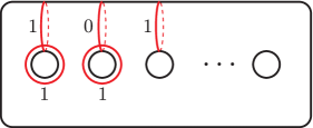
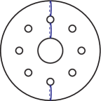
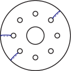
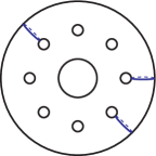
Every odd g3𝑔3g\geq 3: We have a decomposition Σg=Σ11Σ12Σ12Σ11subscriptΣ𝑔superscriptsubscriptΣ11superscriptsubscriptΣ12superscriptsubscriptΣ12superscriptsubscriptΣ11\Sigma_{g}=\Sigma_{1}^{1}\cup\Sigma_{1}^{2}\cup\ldots\cup\Sigma_{1}^{2}\cup\Sigma_{1}^{1}, with 2k12𝑘12k-1 copies of Σ12superscriptsubscriptΣ12\Sigma_{1}^{2} for g=2k+1𝑔2𝑘1g=2k+1. Let A𝐴A denote the 222–chain relation (tc1tc2)6tδ1superscriptsubscript𝑡subscript𝑐1subscript𝑡subscript𝑐26superscriptsubscript𝑡𝛿1(t_{c_{1}}t_{c_{2}})^{6}t_{\delta}^{-1} and B𝐵B denote the 333–chain relation (tc1tc2tc3)4tδ11tδ21superscriptsubscript𝑡subscript𝑐1subscript𝑡subscript𝑐2subscript𝑡subscript𝑐34superscriptsubscript𝑡subscript𝛿11superscriptsubscript𝑡subscript𝛿21(t_{c_{1}}t_{c_{2}}t_{c_{3}})^{4}t_{\delta_{1}}^{-1}t_{\delta_{2}}^{-1}. Embed A𝐴A in both copies of Σ11superscriptsubscriptΣ11\Sigma_{1}^{1}, and embed B1superscript𝐵1B^{-1} into the first copy of Σ12superscriptsubscriptΣ12\Sigma_{1}^{2}, B𝐵B into the second copy, and keep alternating the embeddings in the same fashion for all the copies of Σ12superscriptsubscriptΣ12\Sigma_{1}^{2}. The embeddings of the boundary twists tδ,tδ1,tδ2subscript𝑡𝛿subscript𝑡subscript𝛿1subscript𝑡subscript𝛿2t_{\delta},t_{\delta_{1}},t_{\delta_{2}} all cancel out with each other. So we get an achiral fibration (Yg,fg)subscript𝑌𝑔subscript𝑓𝑔(Y_{g},f_{g}), for g=2k+1𝑔2𝑘1g=2k+1, with only non-separating monodromy curves as in Figure 4(a). Take the quadratic form q𝑞q which maps qg(αi)=qg(βi)=1subscript𝑞𝑔subscript𝛼𝑖subscript𝑞𝑔subscript𝛽𝑖1q_{g}(\alpha_{i})=q_{g}(\beta_{i})=1 for all i𝑖i, so q𝑞q maps all the monodromy curves to 111. By [21], taking the algebraic sum of the signatures of the relations σ(A)=7𝜎𝐴7\sigma(A)=-7 and σ(B)=6𝜎𝐵6\sigma(B)=-6, we calculate that σ(Yg)=2(7)+k(6)+(k1)(6)=8𝜎subscript𝑌𝑔27𝑘6𝑘168\sigma(Y_{g})=2(-7)+k(6)+(k-1)(-6)=-8.

Every even g4𝑔4g\geq 4: This time we have a decomposition Σg=Σ11Σ12Σ12Σ21subscriptΣ𝑔superscriptsubscriptΣ11superscriptsubscriptΣ12superscriptsubscriptΣ12superscriptsubscriptΣ21\Sigma_{g}=\Sigma_{1}^{1}\cup\Sigma_{1}^{2}\cup\ldots\cup\Sigma_{1}^{2}\cup\Sigma_{2}^{1}, with 2k12𝑘12k-1 copies of Σ12superscriptsubscriptΣ12\Sigma_{1}^{2} for g=2k+2𝑔2𝑘2g=2k+2. Let A𝐴A and B𝐵B denote the 222–chain and 333–chain relations as above, and in addition, let C𝐶C denote the 444–chain relation (tc1tc2tc3tc4)10tδ1superscriptsubscript𝑡subscript𝑐1subscript𝑡subscript𝑐2subscript𝑡subscript𝑐3subscript𝑡subscript𝑐410superscriptsubscript𝑡𝛿1(t_{c_{1}}t_{c_{2}}t_{c_{3}}t_{c_{4}})^{10}\,t_{\delta}^{-1}. Embed A𝐴A into Σ11superscriptsubscriptΣ11\Sigma_{1}^{1}, then B1superscript𝐵1B^{-1} and B𝐵B into the copies of Σ12superscriptsubscriptΣ12\Sigma_{1}^{2} in the same alternating fashion as above. This time we finish with embedding C𝐶C into the last Σ21superscriptsubscriptΣ21\Sigma_{2}^{1} piece. Once again, the embeddings of the boundary twists tδ,tδ1,tδ2subscript𝑡𝛿subscript𝑡subscript𝛿1subscript𝑡subscript𝛿2t_{\delta},t_{\delta_{1}},t_{\delta_{2}} all cancel out with each other, and we get an achiral fibration (Yg,fg)subscript𝑌𝑔subscript𝑓𝑔(Y_{g},f_{g}), for g=2k+2𝑔2𝑘2g=2k+2, with non-separating monodromy curves as in Figure 4(b). Take the quadratic form qgsubscript𝑞𝑔q_{g} which maps all qg(αi)=qg(βj)=1subscript𝑞𝑔subscript𝛼𝑖subscript𝑞𝑔subscript𝛽𝑗1q_{g}(\alpha_{i})=q_{g}(\beta_{j})=1 except for qg(βg1)=0subscript𝑞𝑔subscript𝛽𝑔10q_{g}(\beta_{g-1})=0. One can see that all the monodromy curves are mapped to 111 under qgsubscript𝑞𝑔q_{g}. Using [21] again, by taking the algebraic sum of the signatures of the relations σ(A)=7𝜎𝐴7\sigma(A)=-7, σ(B)=6𝜎𝐵6\sigma(B)=-6 and σ(C)=23𝜎𝐶23\sigma(C)=-23, we calculate that σ(Yg)=(7)+k(6)+(k1)(6)+(23)=24𝜎subscript𝑌𝑔7𝑘6𝑘162324\sigma(Y_{g})=(-7)+k(6)+(k-1)(-6)+(-23)=-24.

It is easy to check that the quadratic forms we described for each fibration (Yg,fg)subscript𝑌𝑔subscript𝑓𝑔(Y_{g},f_{g}) has Arf invariant 111. (In fact there is a unique quadratic form for each one, since the monodromy curves of each fgsubscript𝑓𝑔f_{g} generate H1(Σg;2)subscript𝐻1subscriptΣ𝑔subscript2H_{1}(\Sigma_{g};\mathbb{Z}_{2}).) Finally, note that every (Yg,fg)subscript𝑌𝑔subscript𝑓𝑔(Y_{g},f_{g}) has exceptional sections: This is obvious for g=1,2𝑔12g=1,2, and the higher genera ones always have an exceptional section supported in the Σ11superscriptsubscriptΣ11\Sigma_{1}^{1} piece (for instance since the 222–chain is obtained from the 333–chain by capping off a boundary component which has a single Dehn twist). So each (Yg,fg)subscript𝑌𝑔subscript𝑓𝑔(Y_{g},f_{g}) has a section Sgsubscript𝑆𝑔S_{g} of odd self-intersection (in fact a lot of them). ∎

Refer to caption
(a) Odd genus model.
Refer to caption
(b) Even genus model.
Figure 4. Model spin achiral Lefschetz fibrations.
Remark 10.

The converse to the statement of Theorem 9 is not true. For instance, when we double the capped off even-chain relation on ΣgsubscriptΣ𝑔\Sigma_{g} with g0𝑔0g\equiv 0 or 333 (mod 4), we get a spin Lefschetz fibration with signature divisible by 161616, but the only possible quadratic form on ΣgsubscriptΣ𝑔\Sigma_{g}, under which all the monodromy curves are mapped to 111, has Arf invariant 00. On the other hand, when rank(H1(X;2))>0ranksuperscript𝐻1𝑋subscript20\textrm{rank}(H^{1}(X;\mathbb{Z}_{2}))>0, one often finds spin structures on (X,f)𝑋𝑓(X,f) coming from quadratic forms on the fiber ΣgsubscriptΣ𝑔\Sigma_{g} with either Arf invariant, which will be the case for our key example given in Theorem 14. (While this is often the case, it is not always true either; the double of the genus g=2m+1𝑔2𝑚1g=2m+1 Matsumoto-Cadavid-Korkmaz fibration on (Σm×S2)#8¯2(\Sigma_{m}\times S^{2})\,\#8\overline{\mathbb{CP}}{}^{2} has 22msuperscript22𝑚2^{2m} distinct spin structures, but a calculation similar to ours in Example 7 shows that all of these spin structures come from a quadratic form on ΣgsubscriptΣ𝑔\Sigma_{g} with Arf invariant 111!)

Remark 11.

While the achiral Lefschetz fibrations (Yg,fg)subscript𝑌𝑔subscript𝑓𝑔(Y_{g},f_{g}) we built in the proof of Theorem 9 might be of some interest, the 444–manifolds Ygsubscript𝑌𝑔Y_{g} themselves, as well as their spin doubles can all be seen to decompose into a connected sum of standard simply-connected 444–manifolds S2×S2superscript𝑆2superscript𝑆2S^{2}\times S^{2}, 2{\mathbb{CP}}{}^{2} and K3K3{\rm K3}–surface, taken with either orientations. To see this, first observe that they are all fiber sums of 444–manifolds that are such connected sums themselves, along embedded spheres of opposite self-intersections (coming from canceling boundary twists), then apply classical cobordism arguments due to Mandelbaum and Moishezon, as in [40, 29, 11]. In particular, none of them are symplectic when g>2𝑔2g>2.

3. Lefschetz fibrations with signature zero

We will construct our examples of signature zero Lefschetz fibrations in three steps, split into the next three subsections herein, where we employ the breeding technique [12] in increasing complexity, to build signature zero Lefschetz pencils and fibrations out of lower genera pencils. This is done through careful embeddings of the corresponding positive factorizations into the mapping class group of higher genera surfaces, so that one can cancel all the negative Dehn twists against positive ones. Our 333-step construction will result in the signature zero genus–999 Lefschetz fibration (X,f)𝑋𝑓(X,f) of Theorem 14.

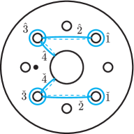
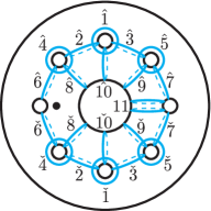
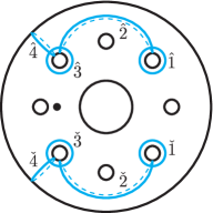
The interested reader can see how the key signature zero example (X,f)𝑋𝑓(X,f) comes to life, without getting bogged down in more technical details. Here is the outline of our construction: We first build the relation (7) in Mod(Σ24)ModsuperscriptsubscriptΣ24\operatorname{Mod}(\Sigma_{2}^{4}) for a genus–222 pencil, using the 222–chain and several lantern relations. We embed two copies of this particular relation into Mod(Σ34)ModsuperscriptsubscriptΣ34\operatorname{Mod}(\Sigma_{3}^{4}), as shown in Figure 12, in order to obtain a new relation for a genus–333 pencil. Importantly, this relation (9) contains positive Dehn twists along four bounding pairs given in Figure 13, each one of which cobound two copies of Σ14superscriptsubscriptΣ14\Sigma_{1}^{4} with a pair of negative Dehn twist curves corresponding to the base points of the pencil. We then embed two copies of this special relation into Mod(Σ9)ModsubscriptΣ9\operatorname{Mod}(\Sigma_{9}) as in Figure 16. At this point we have four pairs of negative Dehn twists, which we will cancel one pair at a time, by carefully embedding four more copies of the same genus–333 relation, so that each time pairs of negative boundary twists match and cancel with positive bounding pair twists of the first two original genus–333 relations, while a positive bounding pair matches and cancels with a negative pair. Here one simply needs to see how the positive bounding pairs from the top and the bottom halves of Σ9subscriptΣ9\Sigma_{9} in Figure 16 cobound a Σ34superscriptsubscriptΣ34\Sigma_{3}^{4}, split into two copies of Σ14superscriptsubscriptΣ14\Sigma_{1}^{4}, cobounded by these positive pairs and a negative pair from the first two embeddings of the genus–333 relation. Following the ingenious work of Endo and Nagami [21], which allows one to calculate the signature of a Lefschetz fibration via elementary relations in the mapping class group, a simple algebraic count of the total number of 222–chain and lantern relations we employed (as cancellations and braid relations do not affect the signature) confirms that the genus–222 and genus–333 pencils, and the genus–999 Lefschetz fibration we built at the end, all have signature zero.

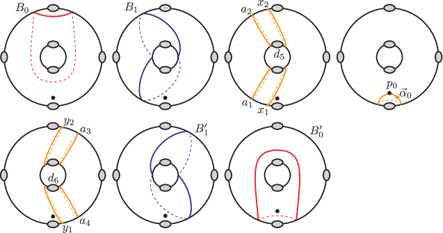
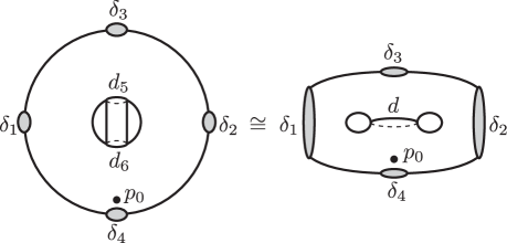
During our 333–step construction we will also chase around an additional marked point on the fiber, the information on which we will need only later when calculating the divisibility of the fiber class of (X,f)𝑋𝑓(X,f). The reader who is not interested in this particular calculation can safely ignore the additional point-pushing maps that appear in our monodromy factorizations. In fact, while the breeding technique plays an innovative role in the construction of (X,f)𝑋𝑓(X,f), because we present this fibration with an explicit positive factorization, the more conservative reader may choose to skip the next three subsections and verify its monodromy given in Theorem 14 in a straightforward fashion, using the Alexander method. (This is a tedious but still manageable calculation, as we have observed so while doing our due diligence to test our monodromy using the same method.)

3.1. A signature zero genus–222 pencil

We begin with describing a genus–222 Lefschetz pencil, whose topology and monodromy both have special features we need for the later steps of our construction. Namely, we would like the total space to have signature zero and be spin, and the monodromy curves to contain a bounding pair and two disjoint separating curves. (The need for all these properties will become clear as we move on to next steps.)

In order to make our construction as self-contained as possible, we will derive all our relations from elementary relations that are known to generate the mapping class group, namely, the 222–chain relation, the lantern relation, and the braid relation, along with commutativity, cancellation and conjugation. In the computations we will freely perform Hurwitz moves and cyclic permutations without stating explicitly.

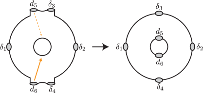
A variation of the 666–holed torus relation: We first present a variation of what is known as the 666–holed torus relation. The curves involved in our construction to follow are given in Figure 5(a).

Refer to caption
(a) The 222-chain relation and lantern relations.
Refer to caption
(b) Rearrangement of the boundary components.
Figure 5. Construction of a 666–holed torus relation.

We begin with the following 222–chain relation and lantern relation:

(t\scaletoa19ptt\scaletob9pt)subscript𝑡\scaletosubscript𝑎19𝑝𝑡subscript𝑡\scaleto𝑏9𝑝𝑡\displaystyle(t_{\scaleto{\mathstrut a_{1}}{9pt}}t_{\scaleto{\mathstrut b}{9pt}}) =t\scaletod9pt,absentsubscript𝑡\scaleto𝑑9𝑝𝑡\displaystyle=t_{\scaleto{\mathstrut d}{9pt}},
t\scaletoa39ptt\scaletod9ptt\scaletoγ9ptsubscript𝑡\scaletosubscript𝑎39𝑝𝑡subscript𝑡\scaleto𝑑9𝑝𝑡subscript𝑡\scaleto𝛾9𝑝𝑡\displaystyle t_{\scaleto{\mathstrut a_{3}}{9pt}}t_{\scaleto{\mathstrut d}{9pt}}t_{\scaleto{\mathstrut\gamma}{9pt}} =t\scaletoa19ptt\scaletoa19ptt\scaletod19ptt\scaletod29pt.absentsubscript𝑡\scaletosubscript𝑎19𝑝𝑡subscript𝑡\scaletosubscript𝑎19𝑝𝑡subscript𝑡\scaletosubscript𝑑19𝑝𝑡subscript𝑡\scaletosubscript𝑑29𝑝𝑡\displaystyle=t_{\scaleto{\mathstrut a_{1}}{9pt}}t_{\scaleto{\mathstrut a_{1}}{9pt}}t_{\scaleto{\mathstrut d_{1}}{9pt}}t_{\scaleto{\mathstrut d_{2}}{9pt}}.

We combine them as follows. (Here we underline the parts that we modify in that very step.)

11\displaystyle 1 =t\scaletoa19ptt\scaletob9ptt\scaletoa19ptt\scaletob9ptt\scaletoa19ptt\scaletob9ptt\scaletoa19ptt\scaletob9ptt\scaletoa19ptt\scaletob9ptt\scaletoa19ptt\scaletob9ptt\scaletod9pt1t\scaletod9ptt\scaletoγ9ptt\scaletoa39ptt\scaletoa19pt1t\scaletoa19pt1t\scaletod19pt1t\scaletod29pt1absentsubscript𝑡\scaletosubscript𝑎19𝑝𝑡subscript𝑡\scaleto𝑏9𝑝𝑡subscript𝑡\scaletosubscript𝑎19𝑝𝑡subscript𝑡\scaleto𝑏9𝑝𝑡subscript𝑡\scaletosubscript𝑎19𝑝𝑡subscript𝑡\scaleto𝑏9𝑝𝑡subscript𝑡\scaletosubscript𝑎19𝑝𝑡subscript𝑡\scaleto𝑏9𝑝𝑡subscript𝑡\scaletosubscript𝑎19𝑝𝑡subscript𝑡\scaleto𝑏9𝑝𝑡subscript𝑡\scaletosubscript𝑎19𝑝𝑡subscript𝑡\scaleto𝑏9𝑝𝑡superscriptsubscript𝑡\scaleto𝑑9𝑝𝑡1subscript𝑡\scaleto𝑑9𝑝𝑡subscript𝑡\scaleto𝛾9𝑝𝑡subscript𝑡\scaletosubscript𝑎39𝑝𝑡superscriptsubscript𝑡\scaletosubscript𝑎19𝑝𝑡1superscriptsubscript𝑡\scaletosubscript𝑎19𝑝𝑡1superscriptsubscript𝑡\scaletosubscript𝑑19𝑝𝑡1superscriptsubscript𝑡\scaletosubscript𝑑29𝑝𝑡1\displaystyle=t_{\scaleto{\mathstrut a_{1}}{9pt}}t_{\scaleto{\mathstrut b}{9pt}}t_{\scaleto{\mathstrut a_{1}}{9pt}}t_{\scaleto{\mathstrut b}{9pt}}t_{\scaleto{\mathstrut a_{1}}{9pt}}t_{\scaleto{\mathstrut b}{9pt}}t_{\scaleto{\mathstrut a_{1}}{9pt}}t_{\scaleto{\mathstrut b}{9pt}}t_{\scaleto{\mathstrut a_{1}}{9pt}}t_{\scaleto{\mathstrut b}{9pt}}t_{\scaleto{\mathstrut a_{1}}{9pt}}t_{\scaleto{\mathstrut b}{9pt}}t_{\scaleto{\mathstrut d}{9pt}}^{-1}\cdot t_{\scaleto{\mathstrut d}{9pt}}t_{\scaleto{\mathstrut\gamma}{9pt}}t_{\scaleto{\mathstrut a_{3}}{9pt}}t_{\scaleto{\mathstrut a_{1}}{9pt}}^{-1}t_{\scaleto{\mathstrut a_{1}}{9pt}}^{-1}t_{\scaleto{\mathstrut d_{1}}{9pt}}^{-1}t_{\scaleto{\mathstrut d_{2}}{9pt}}^{-1}
=t\scaletoa19ptt\scaletob9ptt\scaletoa19ptt\scaletob9ptt\scaletoa19ptt\scaletob9ptt\scaletoa19ptt\scaletob9ptt\scaletod9pt1t\scaletod9ptt\scaletoγ9ptt\scaletoa39ptt\scaletoa19pt1t\scaletoa19pt1t\scaletod19pt1t\scaletod29pt1t\scaletoa19ptt\scaletob9ptt\scaletoa19ptt\scaletob9ptabsentsubscript𝑡\scaletosubscript𝑎19𝑝𝑡subscript𝑡\scaleto𝑏9𝑝𝑡subscript𝑡\scaletosubscript𝑎19𝑝𝑡subscript𝑡\scaleto𝑏9𝑝𝑡subscript𝑡\scaletosubscript𝑎19𝑝𝑡subscript𝑡\scaleto𝑏9𝑝𝑡subscript𝑡\scaletosubscript𝑎19𝑝𝑡subscript𝑡\scaleto𝑏9𝑝𝑡superscriptsubscript𝑡\scaleto𝑑9𝑝𝑡1subscript𝑡\scaleto𝑑9𝑝𝑡subscript𝑡\scaleto𝛾9𝑝𝑡subscript𝑡\scaletosubscript𝑎39𝑝𝑡superscriptsubscript𝑡\scaletosubscript𝑎19𝑝𝑡1superscriptsubscript𝑡\scaletosubscript𝑎19𝑝𝑡1superscriptsubscript𝑡\scaletosubscript𝑑19𝑝𝑡1superscriptsubscript𝑡\scaletosubscript𝑑29𝑝𝑡1subscript𝑡\scaletosubscript𝑎19𝑝𝑡subscript𝑡\scaleto𝑏9𝑝𝑡subscript𝑡\scaletosubscript𝑎19𝑝𝑡subscript𝑡\scaleto𝑏9𝑝𝑡\displaystyle=t_{\scaleto{\mathstrut a_{1}}{9pt}}t_{\scaleto{\mathstrut b}{9pt}}t_{\scaleto{\mathstrut a_{1}}{9pt}}t_{\scaleto{\mathstrut b}{9pt}}t_{\scaleto{\mathstrut a_{1}}{9pt}}t_{\scaleto{\mathstrut b}{9pt}}t_{\scaleto{\mathstrut a_{1}}{9pt}}t_{\scaleto{\mathstrut b}{9pt}}t_{\scaleto{\mathstrut d}{9pt}}^{-1}\cdot t_{\scaleto{\mathstrut d}{9pt}}t_{\scaleto{\mathstrut\gamma}{9pt}}t_{\scaleto{\mathstrut a_{3}}{9pt}}t_{\scaleto{\mathstrut a_{1}}{9pt}}^{-1}t_{\scaleto{\mathstrut a_{1}}{9pt}}^{-1}t_{\scaleto{\mathstrut d_{1}}{9pt}}^{-1}t_{\scaleto{\mathstrut d_{2}}{9pt}}^{-1}\cdot t_{\scaleto{\mathstrut a_{1}}{9pt}}t_{\scaleto{\mathstrut b}{9pt}}t_{\scaleto{\mathstrut a_{1}}{9pt}}t_{\scaleto{\mathstrut b}{9pt}}
=t\scaletoa19ptt\scaletob9ptt\scaletoa19ptt\scaletob9ptt\scaletoa19ptt\scaletob9ptt\scaletoa19ptt\scaletob9ptt\scaletod9pt1t\scaletod9ptt\scaletoγ9ptt\scaletoa39ptt\scaletoa19pt1t\scaletoa19pt1t\scaletoa19ptt\scaletob9ptt\scaletoa19ptt\scaletob9ptt\scaletod19pt1t\scaletod29pt1absentsubscript𝑡\scaletosubscript𝑎19𝑝𝑡subscript𝑡\scaleto𝑏9𝑝𝑡subscript𝑡\scaletosubscript𝑎19𝑝𝑡subscript𝑡\scaleto𝑏9𝑝𝑡subscript𝑡\scaletosubscript𝑎19𝑝𝑡subscript𝑡\scaleto𝑏9𝑝𝑡subscript𝑡\scaletosubscript𝑎19𝑝𝑡subscript𝑡\scaleto𝑏9𝑝𝑡superscriptsubscript𝑡\scaleto𝑑9𝑝𝑡1subscript𝑡\scaleto𝑑9𝑝𝑡subscript𝑡\scaleto𝛾9𝑝𝑡subscript𝑡\scaletosubscript𝑎39𝑝𝑡superscriptsubscript𝑡\scaletosubscript𝑎19𝑝𝑡1superscriptsubscript𝑡\scaletosubscript𝑎19𝑝𝑡1subscript𝑡\scaletosubscript𝑎19𝑝𝑡subscript𝑡\scaleto𝑏9𝑝𝑡subscript𝑡\scaletosubscript𝑎19𝑝𝑡subscript𝑡\scaleto𝑏9𝑝𝑡superscriptsubscript𝑡\scaletosubscript𝑑19𝑝𝑡1superscriptsubscript𝑡\scaletosubscript𝑑29𝑝𝑡1\displaystyle=t_{\scaleto{\mathstrut a_{1}}{9pt}}t_{\scaleto{\mathstrut b}{9pt}}t_{\scaleto{\mathstrut a_{1}}{9pt}}t_{\scaleto{\mathstrut b}{9pt}}t_{\scaleto{\mathstrut a_{1}}{9pt}}t_{\scaleto{\mathstrut b}{9pt}}t_{\scaleto{\mathstrut a_{1}}{9pt}}t_{\scaleto{\mathstrut b}{9pt}}t_{\scaleto{\mathstrut d}{9pt}}^{-1}\cdot t_{\scaleto{\mathstrut d}{9pt}}t_{\scaleto{\mathstrut\gamma}{9pt}}t_{\scaleto{\mathstrut a_{3}}{9pt}}t_{\scaleto{\mathstrut a_{1}}{9pt}}^{-1}t_{\scaleto{\mathstrut a_{1}}{9pt}}^{-1}\cdot t_{\scaleto{\mathstrut a_{1}}{9pt}}t_{\scaleto{\mathstrut b}{9pt}}t_{\scaleto{\mathstrut a_{1}}{9pt}}t_{\scaleto{\mathstrut b}{9pt}}\cdot t_{\scaleto{\mathstrut d_{1}}{9pt}}^{-1}t_{\scaleto{\mathstrut d_{2}}{9pt}}^{-1}
=t\scaletoa19ptt\scaletob9ptt\scaletoa19ptt\scaletob9ptt\scaletoa19ptt\scaletob9ptt\scaletoa19ptt\scaletob9ptt\scaletoγ9ptt\scaletoa39ptt\scaletoa19pt1t\scaletob9ptt\scaletoa19ptt\scaletob9pt¯t\scaletod19pt1t\scaletod29pt1absentsubscript𝑡\scaletosubscript𝑎19𝑝𝑡subscript𝑡\scaleto𝑏9𝑝𝑡subscript𝑡\scaletosubscript𝑎19𝑝𝑡subscript𝑡\scaleto𝑏9𝑝𝑡subscript𝑡\scaletosubscript𝑎19𝑝𝑡subscript𝑡\scaleto𝑏9𝑝𝑡subscript𝑡\scaletosubscript𝑎19𝑝𝑡subscript𝑡\scaleto𝑏9𝑝𝑡subscript𝑡\scaleto𝛾9𝑝𝑡subscript𝑡\scaletosubscript𝑎39𝑝𝑡superscriptsubscript𝑡\scaletosubscript𝑎19𝑝𝑡1¯subscript𝑡\scaleto𝑏9𝑝𝑡subscript𝑡\scaletosubscript𝑎19𝑝𝑡subscript𝑡\scaleto𝑏9𝑝𝑡superscriptsubscript𝑡\scaletosubscript𝑑19𝑝𝑡1superscriptsubscript𝑡\scaletosubscript𝑑29𝑝𝑡1\displaystyle=t_{\scaleto{\mathstrut a_{1}}{9pt}}t_{\scaleto{\mathstrut b}{9pt}}t_{\scaleto{\mathstrut a_{1}}{9pt}}t_{\scaleto{\mathstrut b}{9pt}}t_{\scaleto{\mathstrut a_{1}}{9pt}}t_{\scaleto{\mathstrut b}{9pt}}t_{\scaleto{\mathstrut a_{1}}{9pt}}t_{\scaleto{\mathstrut b}{9pt}}t_{\scaleto{\mathstrut\gamma}{9pt}}t_{\scaleto{\mathstrut a_{3}}{9pt}}t_{\scaleto{\mathstrut a_{1}}{9pt}}^{-1}\underline{t_{\scaleto{\mathstrut b}{9pt}}t_{\scaleto{\mathstrut a_{1}}{9pt}}t_{\scaleto{\mathstrut b}{9pt}}}\cdot t_{\scaleto{\mathstrut d_{1}}{9pt}}^{-1}t_{\scaleto{\mathstrut d_{2}}{9pt}}^{-1}
=t\scaletoa19ptt\scaletob9ptt\scaletoa19ptt\scaletob9ptt\scaletoa19ptt\scaletob9ptt\scaletoa19ptt\scaletob9ptt\scaletoγ9ptt\scaletoa39ptt\scaletoa19pt1t\scaletoa19ptt\scaletob9ptt\scaletoa19ptt\scaletod19pt1t\scaletod29pt1absentsubscript𝑡\scaletosubscript𝑎19𝑝𝑡subscript𝑡\scaleto𝑏9𝑝𝑡subscript𝑡\scaletosubscript𝑎19𝑝𝑡subscript𝑡\scaleto𝑏9𝑝𝑡subscript𝑡\scaletosubscript𝑎19𝑝𝑡subscript𝑡\scaleto𝑏9𝑝𝑡subscript𝑡\scaletosubscript𝑎19𝑝𝑡subscript𝑡\scaleto𝑏9𝑝𝑡subscript𝑡\scaleto𝛾9𝑝𝑡subscript𝑡\scaletosubscript𝑎39𝑝𝑡superscriptsubscript𝑡\scaletosubscript𝑎19𝑝𝑡1subscript𝑡\scaletosubscript𝑎19𝑝𝑡subscript𝑡\scaleto𝑏9𝑝𝑡subscript𝑡\scaletosubscript𝑎19𝑝𝑡superscriptsubscript𝑡\scaletosubscript𝑑19𝑝𝑡1superscriptsubscript𝑡\scaletosubscript𝑑29𝑝𝑡1\displaystyle=t_{\scaleto{\mathstrut a_{1}}{9pt}}t_{\scaleto{\mathstrut b}{9pt}}t_{\scaleto{\mathstrut a_{1}}{9pt}}t_{\scaleto{\mathstrut b}{9pt}}t_{\scaleto{\mathstrut a_{1}}{9pt}}t_{\scaleto{\mathstrut b}{9pt}}t_{\scaleto{\mathstrut a_{1}}{9pt}}t_{\scaleto{\mathstrut b}{9pt}}t_{\scaleto{\mathstrut\gamma}{9pt}}t_{\scaleto{\mathstrut a_{3}}{9pt}}t_{\scaleto{\mathstrut a_{1}}{9pt}}^{-1}t_{\scaleto{\mathstrut a_{1}}{9pt}}t_{\scaleto{\mathstrut b}{9pt}}t_{\scaleto{\mathstrut a_{1}}{9pt}}\cdot t_{\scaleto{\mathstrut d_{1}}{9pt}}^{-1}t_{\scaleto{\mathstrut d_{2}}{9pt}}^{-1}
=t\scaletoa19ptt\scaletob9ptt\scaletoa19ptt\scaletob9ptt\scaletoa19ptt\scaletob9ptt\scaletoa19ptt\scaletob9ptt\scaletoγ9pt¯t\scaletoa39ptt\scaletob9ptt\scaletoa19ptt\scaletod19pt1t\scaletod29pt1absentsubscript𝑡\scaletosubscript𝑎19𝑝𝑡subscript𝑡\scaleto𝑏9𝑝𝑡subscript𝑡\scaletosubscript𝑎19𝑝𝑡¯subscript𝑡\scaleto𝑏9𝑝𝑡subscript𝑡\scaletosubscript𝑎19𝑝𝑡subscript𝑡\scaleto𝑏9𝑝𝑡subscript𝑡\scaletosubscript𝑎19𝑝𝑡subscript𝑡\scaleto𝑏9𝑝𝑡subscript𝑡\scaleto𝛾9𝑝𝑡subscript𝑡\scaletosubscript𝑎39𝑝𝑡subscript𝑡\scaleto𝑏9𝑝𝑡subscript𝑡\scaletosubscript𝑎19𝑝𝑡superscriptsubscript𝑡\scaletosubscript𝑑19𝑝𝑡1superscriptsubscript𝑡\scaletosubscript𝑑29𝑝𝑡1\displaystyle=t_{\scaleto{\mathstrut a_{1}}{9pt}}t_{\scaleto{\mathstrut b}{9pt}}t_{\scaleto{\mathstrut a_{1}}{9pt}}\underline{t_{\scaleto{\mathstrut b}{9pt}}t_{\scaleto{\mathstrut a_{1}}{9pt}}t_{\scaleto{\mathstrut b}{9pt}}t_{\scaleto{\mathstrut a_{1}}{9pt}}t_{\scaleto{\mathstrut b}{9pt}}t_{\scaleto{\mathstrut\gamma}{9pt}}}t_{\scaleto{\mathstrut a_{3}}{9pt}}t_{\scaleto{\mathstrut b}{9pt}}t_{\scaleto{\mathstrut a_{1}}{9pt}}\cdot t_{\scaleto{\mathstrut d_{1}}{9pt}}^{-1}t_{\scaleto{\mathstrut d_{2}}{9pt}}^{-1}
=t\scaletoa19ptt\scaletob9ptt\scaletoa19ptt\scaletoa39ptt\scaletob9ptt\scaletoa19ptt\scaletob9ptt\scaletoa19ptt\scaletob9ptt\scaletoa39ptt\scaletob9ptt\scaletoa19ptt\scaletod19pt1t\scaletod29pt1absentsubscript𝑡\scaletosubscript𝑎19𝑝𝑡subscript𝑡\scaleto𝑏9𝑝𝑡subscript𝑡\scaletosubscript𝑎19𝑝𝑡subscript𝑡\scaletosubscript𝑎39𝑝𝑡subscript𝑡\scaleto𝑏9𝑝𝑡subscript𝑡\scaletosubscript𝑎19𝑝𝑡subscript𝑡\scaleto𝑏9𝑝𝑡subscript𝑡\scaletosubscript𝑎19𝑝𝑡subscript𝑡\scaleto𝑏9𝑝𝑡subscript𝑡\scaletosubscript𝑎39𝑝𝑡subscript𝑡\scaleto𝑏9𝑝𝑡subscript𝑡\scaletosubscript𝑎19𝑝𝑡superscriptsubscript𝑡\scaletosubscript𝑑19𝑝𝑡1superscriptsubscript𝑡\scaletosubscript𝑑29𝑝𝑡1\displaystyle=t_{\scaleto{\mathstrut a_{1}}{9pt}}t_{\scaleto{\mathstrut b}{9pt}}t_{\scaleto{\mathstrut a_{1}}{9pt}}t_{\scaleto{\mathstrut a_{3}}{9pt}}t_{\scaleto{\mathstrut b}{9pt}}t_{\scaleto{\mathstrut a_{1}}{9pt}}t_{\scaleto{\mathstrut b}{9pt}}t_{\scaleto{\mathstrut a_{1}}{9pt}}t_{\scaleto{\mathstrut b}{9pt}}t_{\scaleto{\mathstrut a_{3}}{9pt}}t_{\scaleto{\mathstrut b}{9pt}}t_{\scaleto{\mathstrut a_{1}}{9pt}}\cdot t_{\scaleto{\mathstrut d_{1}}{9pt}}^{-1}t_{\scaleto{\mathstrut d_{2}}{9pt}}^{-1}
(Here we used the simple observation that t\scaletob9ptt\scaletoa19ptt\scaletob9ptt\scaletoa19ptt\scaletob9pt(γ)=a3subscript𝑡\scaleto𝑏9𝑝𝑡subscript𝑡\scaletosubscript𝑎19𝑝𝑡subscript𝑡\scaleto𝑏9𝑝𝑡subscript𝑡\scaletosubscript𝑎19𝑝𝑡subscript𝑡\scaleto𝑏9𝑝𝑡𝛾subscript𝑎3t_{\scaleto{\mathstrut b}{9pt}}t_{\scaleto{\mathstrut a_{1}}{9pt}}t_{\scaleto{\mathstrut b}{9pt}}t_{\scaleto{\mathstrut a_{1}}{9pt}}t_{\scaleto{\mathstrut b}{9pt}}(\gamma)=a_{3}.)
=t\scaletoa19ptt\scaletob9ptt\scaletoa19ptt\scaletoa39ptt\scaletob9ptt\scaletoa19ptt\scaletob9ptt\scaletoa19ptt\scaletob9ptt\scaletoa39ptt\scaletob9pt¯t\scaletoa19ptt\scaletod19pt1t\scaletod29pt1absentsubscript𝑡\scaletosubscript𝑎19𝑝𝑡subscript𝑡\scaleto𝑏9𝑝𝑡subscript𝑡\scaletosubscript𝑎19𝑝𝑡subscript𝑡\scaletosubscript𝑎39𝑝𝑡subscript𝑡\scaleto𝑏9𝑝𝑡subscript𝑡\scaletosubscript𝑎19𝑝𝑡subscript𝑡\scaleto𝑏9𝑝𝑡subscript𝑡\scaletosubscript𝑎19𝑝𝑡¯subscript𝑡\scaleto𝑏9𝑝𝑡subscript𝑡\scaletosubscript𝑎39𝑝𝑡subscript𝑡\scaleto𝑏9𝑝𝑡subscript𝑡\scaletosubscript𝑎19𝑝𝑡superscriptsubscript𝑡\scaletosubscript𝑑19𝑝𝑡1superscriptsubscript𝑡\scaletosubscript𝑑29𝑝𝑡1\displaystyle=t_{\scaleto{\mathstrut a_{1}}{9pt}}t_{\scaleto{\mathstrut b}{9pt}}t_{\scaleto{\mathstrut a_{1}}{9pt}}t_{\scaleto{\mathstrut a_{3}}{9pt}}t_{\scaleto{\mathstrut b}{9pt}}t_{\scaleto{\mathstrut a_{1}}{9pt}}t_{\scaleto{\mathstrut b}{9pt}}t_{\scaleto{\mathstrut a_{1}}{9pt}}\underline{t_{\scaleto{\mathstrut b}{9pt}}t_{\scaleto{\mathstrut a_{3}}{9pt}}t_{\scaleto{\mathstrut b}{9pt}}}t_{\scaleto{\mathstrut a_{1}}{9pt}}\cdot t_{\scaleto{\mathstrut d_{1}}{9pt}}^{-1}t_{\scaleto{\mathstrut d_{2}}{9pt}}^{-1}
=t\scaletoa19ptt\scaletob9ptt\scaletoa19ptt\scaletoa39ptt\scaletob9ptt\scaletoa19ptt\scaletob9ptt\scaletoa19ptt\scaletoa39ptt\scaletob9ptt\scaletoa39ptt\scaletoa19ptt\scaletod19pt1t\scaletod29pt1absentsubscript𝑡\scaletosubscript𝑎19𝑝𝑡subscript𝑡\scaleto𝑏9𝑝𝑡subscript𝑡\scaletosubscript𝑎19𝑝𝑡subscript𝑡\scaletosubscript𝑎39𝑝𝑡subscript𝑡\scaleto𝑏9𝑝𝑡subscript𝑡\scaletosubscript𝑎19𝑝𝑡subscript𝑡\scaleto𝑏9𝑝𝑡subscript𝑡\scaletosubscript𝑎19𝑝𝑡subscript𝑡\scaletosubscript𝑎39𝑝𝑡subscript𝑡\scaleto𝑏9𝑝𝑡subscript𝑡\scaletosubscript𝑎39𝑝𝑡subscript𝑡\scaletosubscript𝑎19𝑝𝑡superscriptsubscript𝑡\scaletosubscript𝑑19𝑝𝑡1superscriptsubscript𝑡\scaletosubscript𝑑29𝑝𝑡1\displaystyle=t_{\scaleto{\mathstrut a_{1}}{9pt}}t_{\scaleto{\mathstrut b}{9pt}}t_{\scaleto{\mathstrut a_{1}}{9pt}}t_{\scaleto{\mathstrut a_{3}}{9pt}}t_{\scaleto{\mathstrut b}{9pt}}t_{\scaleto{\mathstrut a_{1}}{9pt}}t_{\scaleto{\mathstrut b}{9pt}}t_{\scaleto{\mathstrut a_{1}}{9pt}}t_{\scaleto{\mathstrut a_{3}}{9pt}}t_{\scaleto{\mathstrut b}{9pt}}t_{\scaleto{\mathstrut a_{3}}{9pt}}t_{\scaleto{\mathstrut a_{1}}{9pt}}\cdot t_{\scaleto{\mathstrut d_{1}}{9pt}}^{-1}t_{\scaleto{\mathstrut d_{2}}{9pt}}^{-1}
=t\scaletoa19ptt\scaletob9ptt\scaletoa19ptt\scaletoa39ptt\scaletob9ptt\scaletoa19ptt\scaletob9ptt\scaletoa39ptt\scaletoa19ptt\scaletob9ptt\scaletoa19pt¯t\scaletoa39ptt\scaletod19pt1t\scaletod29pt1absentsubscript𝑡\scaletosubscript𝑎19𝑝𝑡subscript𝑡\scaleto𝑏9𝑝𝑡subscript𝑡\scaletosubscript𝑎19𝑝𝑡subscript𝑡\scaletosubscript𝑎39𝑝𝑡subscript𝑡\scaleto𝑏9𝑝𝑡subscript𝑡\scaletosubscript𝑎19𝑝𝑡subscript𝑡\scaleto𝑏9𝑝𝑡subscript𝑡\scaletosubscript𝑎39𝑝𝑡¯subscript𝑡\scaletosubscript𝑎19𝑝𝑡subscript𝑡\scaleto𝑏9𝑝𝑡subscript𝑡\scaletosubscript𝑎19𝑝𝑡subscript𝑡\scaletosubscript𝑎39𝑝𝑡superscriptsubscript𝑡\scaletosubscript𝑑19𝑝𝑡1superscriptsubscript𝑡\scaletosubscript𝑑29𝑝𝑡1\displaystyle=t_{\scaleto{\mathstrut a_{1}}{9pt}}t_{\scaleto{\mathstrut b}{9pt}}t_{\scaleto{\mathstrut a_{1}}{9pt}}t_{\scaleto{\mathstrut a_{3}}{9pt}}t_{\scaleto{\mathstrut b}{9pt}}t_{\scaleto{\mathstrut a_{1}}{9pt}}t_{\scaleto{\mathstrut b}{9pt}}t_{\scaleto{\mathstrut a_{3}}{9pt}}\underline{t_{\scaleto{\mathstrut a_{1}}{9pt}}t_{\scaleto{\mathstrut b}{9pt}}t_{\scaleto{\mathstrut a_{1}}{9pt}}}t_{\scaleto{\mathstrut a_{3}}{9pt}}\cdot t_{\scaleto{\mathstrut d_{1}}{9pt}}^{-1}t_{\scaleto{\mathstrut d_{2}}{9pt}}^{-1}
=t\scaletoa19ptt\scaletob9ptt\scaletoa19ptt\scaletoa39ptt\scaletob9ptt\scaletoa19ptt\scaletob9ptt\scaletoa39ptt\scaletob9pt¯t\scaletoa19ptt\scaletob9ptt\scaletoa39ptt\scaletod19pt1t\scaletod29pt1absentsubscript𝑡\scaletosubscript𝑎19𝑝𝑡subscript𝑡\scaleto𝑏9𝑝𝑡subscript𝑡\scaletosubscript𝑎19𝑝𝑡subscript𝑡\scaletosubscript𝑎39𝑝𝑡subscript𝑡\scaleto𝑏9𝑝𝑡subscript𝑡\scaletosubscript𝑎19𝑝𝑡¯subscript𝑡\scaleto𝑏9𝑝𝑡subscript𝑡\scaletosubscript𝑎39𝑝𝑡subscript𝑡\scaleto𝑏9𝑝𝑡subscript𝑡\scaletosubscript𝑎19𝑝𝑡subscript𝑡\scaleto𝑏9𝑝𝑡subscript𝑡\scaletosubscript𝑎39𝑝𝑡superscriptsubscript𝑡\scaletosubscript𝑑19𝑝𝑡1superscriptsubscript𝑡\scaletosubscript𝑑29𝑝𝑡1\displaystyle=t_{\scaleto{\mathstrut a_{1}}{9pt}}t_{\scaleto{\mathstrut b}{9pt}}t_{\scaleto{\mathstrut a_{1}}{9pt}}t_{\scaleto{\mathstrut a_{3}}{9pt}}t_{\scaleto{\mathstrut b}{9pt}}t_{\scaleto{\mathstrut a_{1}}{9pt}}\underline{t_{\scaleto{\mathstrut b}{9pt}}t_{\scaleto{\mathstrut a_{3}}{9pt}}t_{\scaleto{\mathstrut b}{9pt}}}t_{\scaleto{\mathstrut a_{1}}{9pt}}t_{\scaleto{\mathstrut b}{9pt}}t_{\scaleto{\mathstrut a_{3}}{9pt}}\cdot t_{\scaleto{\mathstrut d_{1}}{9pt}}^{-1}t_{\scaleto{\mathstrut d_{2}}{9pt}}^{-1}
=t\scaletoa19ptt\scaletob9ptt\scaletoa19ptt\scaletoa39ptt\scaletob9ptt\scaletoa19ptt\scaletoa39ptt\scaletob9ptt\scaletoa39ptt\scaletoa19ptt\scaletob9ptt\scaletoa39ptt\scaletod19pt1t\scaletod29pt1absentsubscript𝑡\scaletosubscript𝑎19𝑝𝑡subscript𝑡\scaleto𝑏9𝑝𝑡subscript𝑡\scaletosubscript𝑎19𝑝𝑡subscript𝑡\scaletosubscript𝑎39𝑝𝑡subscript𝑡\scaleto𝑏9𝑝𝑡subscript𝑡\scaletosubscript𝑎19𝑝𝑡subscript𝑡\scaletosubscript𝑎39𝑝𝑡subscript𝑡\scaleto𝑏9𝑝𝑡subscript𝑡\scaletosubscript𝑎39𝑝𝑡subscript𝑡\scaletosubscript𝑎19𝑝𝑡subscript𝑡\scaleto𝑏9𝑝𝑡subscript𝑡\scaletosubscript𝑎39𝑝𝑡superscriptsubscript𝑡\scaletosubscript𝑑19𝑝𝑡1superscriptsubscript𝑡\scaletosubscript𝑑29𝑝𝑡1\displaystyle=t_{\scaleto{\mathstrut a_{1}}{9pt}}t_{\scaleto{\mathstrut b}{9pt}}t_{\scaleto{\mathstrut a_{1}}{9pt}}t_{\scaleto{\mathstrut a_{3}}{9pt}}t_{\scaleto{\mathstrut b}{9pt}}t_{\scaleto{\mathstrut a_{1}}{9pt}}t_{\scaleto{\mathstrut a_{3}}{9pt}}t_{\scaleto{\mathstrut b}{9pt}}t_{\scaleto{\mathstrut a_{3}}{9pt}}t_{\scaleto{\mathstrut a_{1}}{9pt}}t_{\scaleto{\mathstrut b}{9pt}}t_{\scaleto{\mathstrut a_{3}}{9pt}}\cdot t_{\scaleto{\mathstrut d_{1}}{9pt}}^{-1}t_{\scaleto{\mathstrut d_{2}}{9pt}}^{-1}
=t\scaletoa19ptt\scaletob9ptt\scaletoa19ptt\scaletoa39ptt\scaletod19pt1¯t\scaletob9ptt\scaletoa19ptt\scaletoa39ptt\scaletob9ptt\scaletoa39ptt\scaletoa19ptt\scaletod29pt1¯t\scaletob9ptt\scaletoa39pt.absentsubscript𝑡\scaletosubscript𝑎19𝑝𝑡subscript𝑡\scaleto𝑏9𝑝𝑡¯subscript𝑡\scaletosubscript𝑎19𝑝𝑡subscript𝑡\scaletosubscript𝑎39𝑝𝑡superscriptsubscript𝑡\scaletosubscript𝑑19𝑝𝑡1subscript𝑡\scaleto𝑏9𝑝𝑡subscript𝑡\scaletosubscript𝑎19𝑝𝑡subscript𝑡\scaletosubscript𝑎39𝑝𝑡subscript𝑡\scaleto𝑏9𝑝𝑡¯subscript𝑡\scaletosubscript𝑎39𝑝𝑡subscript𝑡\scaletosubscript𝑎19𝑝𝑡superscriptsubscript𝑡\scaletosubscript𝑑29𝑝𝑡1subscript𝑡\scaleto𝑏9𝑝𝑡subscript𝑡\scaletosubscript𝑎39𝑝𝑡\displaystyle=t_{\scaleto{\mathstrut a_{1}}{9pt}}t_{\scaleto{\mathstrut b}{9pt}}\cdot\underline{t_{\scaleto{\mathstrut a_{1}}{9pt}}t_{\scaleto{\mathstrut a_{3}}{9pt}}t_{\scaleto{\mathstrut d_{1}}{9pt}}^{-1}}\cdot t_{\scaleto{\mathstrut b}{9pt}}t_{\scaleto{\mathstrut a_{1}}{9pt}}t_{\scaleto{\mathstrut a_{3}}{9pt}}t_{\scaleto{\mathstrut b}{9pt}}\cdot\underline{t_{\scaleto{\mathstrut a_{3}}{9pt}}t_{\scaleto{\mathstrut a_{1}}{9pt}}t_{\scaleto{\mathstrut d_{2}}{9pt}}^{-1}}\cdot t_{\scaleto{\mathstrut b}{9pt}}t_{\scaleto{\mathstrut a_{3}}{9pt}}.

Now we substitute the two lantern relations

t\scaletod19ptt\scaletoγ19ptt\scaletoa29pt=t\scaletoa19ptt\scaletoa39ptt\scaletoδ19ptt\scaletod39pt,subscript𝑡\scaletosubscript𝑑19𝑝𝑡subscript𝑡\scaletosubscript𝛾19𝑝𝑡subscript𝑡\scaletosubscript𝑎29𝑝𝑡subscript𝑡\scaletosubscript𝑎19𝑝𝑡subscript𝑡\scaletosubscript𝑎39𝑝𝑡subscript𝑡\scaletosubscript𝛿19𝑝𝑡subscript𝑡\scaletosubscript𝑑39𝑝𝑡\displaystyle t_{\scaleto{\mathstrut d_{1}}{9pt}}t_{\scaleto{\mathstrut\gamma_{1}}{9pt}}t_{\scaleto{\mathstrut a_{2}}{9pt}}=t_{\scaleto{\mathstrut a_{1}}{9pt}}t_{\scaleto{\mathstrut a_{3}}{9pt}}t_{\scaleto{\mathstrut\delta_{1}}{9pt}}t_{\scaleto{\mathstrut d_{3}}{9pt}},
t\scaletod29ptt\scaletoa49ptt\scaletoγ29pt=t\scaletoa19ptt\scaletoa39ptt\scaletoδ29ptt\scaletod49pt,subscript𝑡\scaletosubscript𝑑29𝑝𝑡subscript𝑡\scaletosubscript𝑎49𝑝𝑡subscript𝑡\scaletosubscript𝛾29𝑝𝑡subscript𝑡\scaletosubscript𝑎19𝑝𝑡subscript𝑡\scaletosubscript𝑎39𝑝𝑡subscript𝑡\scaletosubscript𝛿29𝑝𝑡subscript𝑡\scaletosubscript𝑑49𝑝𝑡\displaystyle t_{\scaleto{\mathstrut d_{2}}{9pt}}t_{\scaleto{\mathstrut a_{4}}{9pt}}t_{\scaleto{\mathstrut\gamma_{2}}{9pt}}=t_{\scaleto{\mathstrut a_{1}}{9pt}}t_{\scaleto{\mathstrut a_{3}}{9pt}}t_{\scaleto{\mathstrut\delta_{2}}{9pt}}t_{\scaleto{\mathstrut d_{4}}{9pt}},

to get

11\displaystyle 1 =t\scaletoa19ptt\scaletob9ptt\scaletoa19ptt\scaletoa39ptt\scaletod19pt1t\scaletoa19pt1t\scaletoa39pt1t\scaletod19ptt\scaletoγ19ptt\scaletoa29ptt\scaletoδ19pt1t\scaletod39pt1t\scaletob9ptt\scaletoa19ptt\scaletoa39ptt\scaletob9ptabsentsubscript𝑡\scaletosubscript𝑎19𝑝𝑡subscript𝑡\scaleto𝑏9𝑝𝑡subscript𝑡\scaletosubscript𝑎19𝑝𝑡subscript𝑡\scaletosubscript𝑎39𝑝𝑡superscriptsubscript𝑡\scaletosubscript𝑑19𝑝𝑡1superscriptsubscript𝑡\scaletosubscript𝑎19𝑝𝑡1superscriptsubscript𝑡\scaletosubscript𝑎39𝑝𝑡1subscript𝑡\scaletosubscript𝑑19𝑝𝑡subscript𝑡\scaletosubscript𝛾19𝑝𝑡subscript𝑡\scaletosubscript𝑎29𝑝𝑡superscriptsubscript𝑡\scaletosubscript𝛿19𝑝𝑡1superscriptsubscript𝑡\scaletosubscript𝑑39𝑝𝑡1subscript𝑡\scaleto𝑏9𝑝𝑡subscript𝑡\scaletosubscript𝑎19𝑝𝑡subscript𝑡\scaletosubscript𝑎39𝑝𝑡subscript𝑡\scaleto𝑏9𝑝𝑡\displaystyle=t_{\scaleto{\mathstrut a_{1}}{9pt}}t_{\scaleto{\mathstrut b}{9pt}}\cdot t_{\scaleto{\mathstrut a_{1}}{9pt}}t_{\scaleto{\mathstrut a_{3}}{9pt}}t_{\scaleto{\mathstrut d_{1}}{9pt}}^{-1}\cdot t_{\scaleto{\mathstrut a_{1}}{9pt}}^{-1}t_{\scaleto{\mathstrut a_{3}}{9pt}}^{-1}t_{\scaleto{\mathstrut d_{1}}{9pt}}t_{\scaleto{\mathstrut\gamma_{1}}{9pt}}t_{\scaleto{\mathstrut a_{2}}{9pt}}t_{\scaleto{\mathstrut\delta_{1}}{9pt}}^{-1}t_{\scaleto{\mathstrut d_{3}}{9pt}}^{-1}\cdot t_{\scaleto{\mathstrut b}{9pt}}t_{\scaleto{\mathstrut a_{1}}{9pt}}t_{\scaleto{\mathstrut a_{3}}{9pt}}t_{\scaleto{\mathstrut b}{9pt}}
t\scaletoδ29pt1t\scaletod49pt1t\scaletoa49ptt\scaletoγ29ptt\scaletod29ptt\scaletoa19pt1t\scaletoa39pt1t\scaletoa39ptt\scaletoa19ptt\scaletod29pt1t\scaletob9ptt\scaletoa39pt.absentsuperscriptsubscript𝑡\scaletosubscript𝛿29𝑝𝑡1superscriptsubscript𝑡\scaletosubscript𝑑49𝑝𝑡1subscript𝑡\scaletosubscript𝑎49𝑝𝑡subscript𝑡\scaletosubscript𝛾29𝑝𝑡subscript𝑡\scaletosubscript𝑑29𝑝𝑡superscriptsubscript𝑡\scaletosubscript𝑎19𝑝𝑡1superscriptsubscript𝑡\scaletosubscript𝑎39𝑝𝑡1subscript𝑡\scaletosubscript𝑎39𝑝𝑡subscript𝑡\scaletosubscript𝑎19𝑝𝑡superscriptsubscript𝑡\scaletosubscript𝑑29𝑝𝑡1subscript𝑡\scaleto𝑏9𝑝𝑡subscript𝑡\scaletosubscript𝑎39𝑝𝑡\displaystyle\qquad\cdot t_{\scaleto{\mathstrut\delta_{2}}{9pt}}^{-1}t_{\scaleto{\mathstrut d_{4}}{9pt}}^{-1}t_{\scaleto{\mathstrut a_{4}}{9pt}}t_{\scaleto{\mathstrut\gamma_{2}}{9pt}}t_{\scaleto{\mathstrut d_{2}}{9pt}}t_{\scaleto{\mathstrut a_{1}}{9pt}}^{-1}t_{\scaleto{\mathstrut a_{3}}{9pt}}^{-1}\cdot t_{\scaleto{\mathstrut a_{3}}{9pt}}t_{\scaleto{\mathstrut a_{1}}{9pt}}t_{\scaleto{\mathstrut d_{2}}{9pt}}^{-1}\cdot t_{\scaleto{\mathstrut b}{9pt}}t_{\scaleto{\mathstrut a_{3}}{9pt}}.

Cancellation and commutativity yield

t\scaletoδ19ptt\scaletoδ29ptsubscript𝑡\scaletosubscript𝛿19𝑝𝑡subscript𝑡\scaletosubscript𝛿29𝑝𝑡\displaystyle t_{\scaleto{\mathstrut\delta_{1}}{9pt}}t_{\scaleto{\mathstrut\delta_{2}}{9pt}} =t\scaletoa19ptt\scaletob9ptt\scaletoγ19pt¯t\scaletoa29ptt\scaletob9ptt\scaletoa19ptt\scaletod39pt1t\scaletod49pt1t\scaletoa39ptt\scaletob9ptt\scaletoa49ptt\scaletoγ29ptt\scaletob9ptt\scaletoa39pt¯absent¯subscript𝑡\scaletosubscript𝑎19𝑝𝑡subscript𝑡\scaleto𝑏9𝑝𝑡subscript𝑡\scaletosubscript𝛾19𝑝𝑡subscript𝑡\scaletosubscript𝑎29𝑝𝑡subscript𝑡\scaleto𝑏9𝑝𝑡subscript𝑡\scaletosubscript𝑎19𝑝𝑡superscriptsubscript𝑡\scaletosubscript𝑑39𝑝𝑡1superscriptsubscript𝑡\scaletosubscript𝑑49𝑝𝑡1subscript𝑡\scaletosubscript𝑎39𝑝𝑡subscript𝑡\scaleto𝑏9𝑝𝑡subscript𝑡\scaletosubscript𝑎49𝑝𝑡¯subscript𝑡\scaletosubscript𝛾29𝑝𝑡subscript𝑡\scaleto𝑏9𝑝𝑡subscript𝑡\scaletosubscript𝑎39𝑝𝑡\displaystyle=\underline{t_{\scaleto{\mathstrut a_{1}}{9pt}}t_{\scaleto{\mathstrut b}{9pt}}t_{\scaleto{\mathstrut\gamma_{1}}{9pt}}}t_{\scaleto{\mathstrut a_{2}}{9pt}}t_{\scaleto{\mathstrut b}{9pt}}t_{\scaleto{\mathstrut a_{1}}{9pt}}\cdot t_{\scaleto{\mathstrut d_{3}}{9pt}}^{-1}t_{\scaleto{\mathstrut d_{4}}{9pt}}^{-1}\cdot t_{\scaleto{\mathstrut a_{3}}{9pt}}t_{\scaleto{\mathstrut b}{9pt}}t_{\scaleto{\mathstrut a_{4}}{9pt}}\underline{t_{\scaleto{\mathstrut\gamma_{2}}{9pt}}t_{\scaleto{\mathstrut b}{9pt}}t_{\scaleto{\mathstrut a_{3}}{9pt}}}
=t\scaletoB09ptt\scaletoa19ptt\scaletob9ptt\scaletoa29ptt\scaletob9ptt\scaletoa19ptt\scaletod39pt1t\scaletod49pt1t\scaletoa39ptt\scaletob9ptt\scaletoa49ptt\scaletob9ptt\scaletoa39ptt\scaletoB09ptabsentsubscript𝑡\scaletosubscript𝐵09𝑝𝑡subscript𝑡\scaletosubscript𝑎19𝑝𝑡subscript𝑡\scaleto𝑏9𝑝𝑡subscript𝑡\scaletosubscript𝑎29𝑝𝑡subscript𝑡\scaleto𝑏9𝑝𝑡subscript𝑡\scaletosubscript𝑎19𝑝𝑡superscriptsubscript𝑡\scaletosubscript𝑑39𝑝𝑡1superscriptsubscript𝑡\scaletosubscript𝑑49𝑝𝑡1subscript𝑡\scaletosubscript𝑎39𝑝𝑡subscript𝑡\scaleto𝑏9𝑝𝑡subscript𝑡\scaletosubscript𝑎49𝑝𝑡subscript𝑡\scaleto𝑏9𝑝𝑡subscript𝑡\scaletosubscript𝑎39𝑝𝑡subscript𝑡\scaletosuperscriptsubscript𝐵09𝑝𝑡\displaystyle=t_{\scaleto{\mathstrut B_{0}}{9pt}}t_{\scaleto{\mathstrut a_{1}}{9pt}}t_{\scaleto{\mathstrut b}{9pt}}t_{\scaleto{\mathstrut a_{2}}{9pt}}t_{\scaleto{\mathstrut b}{9pt}}t_{\scaleto{\mathstrut a_{1}}{9pt}}\cdot t_{\scaleto{\mathstrut d_{3}}{9pt}}^{-1}t_{\scaleto{\mathstrut d_{4}}{9pt}}^{-1}\cdot t_{\scaleto{\mathstrut a_{3}}{9pt}}t_{\scaleto{\mathstrut b}{9pt}}t_{\scaleto{\mathstrut a_{4}}{9pt}}t_{\scaleto{\mathstrut b}{9pt}}t_{\scaleto{\mathstrut a_{3}}{9pt}}t_{\scaleto{\mathstrut B_{0}^{\prime}}{9pt}}
where B0:=t\scaletoa19ptt\scaletob9pt(γ1)assignsubscript𝐵0subscript𝑡\scaletosubscript𝑎19𝑝𝑡subscript𝑡\scaleto𝑏9𝑝𝑡subscript𝛾1B_{0}:=t_{\scaleto{\mathstrut a_{1}}{9pt}}t_{\scaleto{\mathstrut b}{9pt}}(\gamma_{1}) and B0:=t\scaletoa39pt1t\scaletob9pt1(γ2)assignsuperscriptsubscript𝐵0superscriptsubscript𝑡\scaletosubscript𝑎39𝑝𝑡1superscriptsubscript𝑡\scaleto𝑏9𝑝𝑡1subscript𝛾2B_{0}^{\prime}:=t_{\scaleto{\mathstrut a_{3}}{9pt}}^{-1}t_{\scaleto{\mathstrut b}{9pt}}^{-1}(\gamma_{2}),
=t\scaletoB09ptt\scaletoa19ptt\scaletob9ptt\scaletoa29ptt\scaletob9pt¯t\scaletoa19ptt\scaletod39pt1t\scaletod49pt1t\scaletoa39ptt\scaletob9ptt\scaletoa49ptt\scaletob9pt¯t\scaletoa39ptt\scaletoB09ptabsentsubscript𝑡\scaletosubscript𝐵09𝑝𝑡subscript𝑡\scaletosubscript𝑎19𝑝𝑡¯subscript𝑡\scaleto𝑏9𝑝𝑡subscript𝑡\scaletosubscript𝑎29𝑝𝑡subscript𝑡\scaleto𝑏9𝑝𝑡subscript𝑡\scaletosubscript𝑎19𝑝𝑡superscriptsubscript𝑡\scaletosubscript𝑑39𝑝𝑡1superscriptsubscript𝑡\scaletosubscript𝑑49𝑝𝑡1subscript𝑡\scaletosubscript𝑎39𝑝𝑡¯subscript𝑡\scaleto𝑏9𝑝𝑡subscript𝑡\scaletosubscript𝑎49𝑝𝑡subscript𝑡\scaleto𝑏9𝑝𝑡subscript𝑡\scaletosubscript𝑎39𝑝𝑡subscript𝑡\scaletosuperscriptsubscript𝐵09𝑝𝑡\displaystyle=t_{\scaleto{\mathstrut B_{0}}{9pt}}t_{\scaleto{\mathstrut a_{1}}{9pt}}\underline{t_{\scaleto{\mathstrut b}{9pt}}t_{\scaleto{\mathstrut a_{2}}{9pt}}t_{\scaleto{\mathstrut b}{9pt}}}t_{\scaleto{\mathstrut a_{1}}{9pt}}\cdot t_{\scaleto{\mathstrut d_{3}}{9pt}}^{-1}t_{\scaleto{\mathstrut d_{4}}{9pt}}^{-1}\cdot t_{\scaleto{\mathstrut a_{3}}{9pt}}\underline{t_{\scaleto{\mathstrut b}{9pt}}t_{\scaleto{\mathstrut a_{4}}{9pt}}t_{\scaleto{\mathstrut b}{9pt}}}t_{\scaleto{\mathstrut a_{3}}{9pt}}t_{\scaleto{\mathstrut B_{0}^{\prime}}{9pt}}
=t\scaletoB09ptt\scaletoa19ptt\scaletoa29ptt\scaletob9pt¯t\scaletoa29ptt\scaletoa19ptt\scaletod39pt1t\scaletod49pt1t\scaletoa39ptt\scaletoa49ptt\scaletob9ptt\scaletoa49ptt\scaletoa39pt¯t\scaletoB09ptabsentsubscript𝑡\scaletosubscript𝐵09𝑝𝑡¯subscript𝑡\scaletosubscript𝑎19𝑝𝑡subscript𝑡\scaletosubscript𝑎29𝑝𝑡subscript𝑡\scaleto𝑏9𝑝𝑡subscript𝑡\scaletosubscript𝑎29𝑝𝑡subscript𝑡\scaletosubscript𝑎19𝑝𝑡superscriptsubscript𝑡\scaletosubscript𝑑39𝑝𝑡1superscriptsubscript𝑡\scaletosubscript𝑑49𝑝𝑡1subscript𝑡\scaletosubscript𝑎39𝑝𝑡subscript𝑡\scaletosubscript𝑎49𝑝𝑡¯subscript𝑡\scaleto𝑏9𝑝𝑡subscript𝑡\scaletosubscript𝑎49𝑝𝑡subscript𝑡\scaletosubscript𝑎39𝑝𝑡subscript𝑡\scaletosuperscriptsubscript𝐵09𝑝𝑡\displaystyle=t_{\scaleto{\mathstrut B_{0}}{9pt}}\underline{t_{\scaleto{\mathstrut a_{1}}{9pt}}t_{\scaleto{\mathstrut a_{2}}{9pt}}t_{\scaleto{\mathstrut b}{9pt}}}t_{\scaleto{\mathstrut a_{2}}{9pt}}t_{\scaleto{\mathstrut a_{1}}{9pt}}\cdot t_{\scaleto{\mathstrut d_{3}}{9pt}}^{-1}t_{\scaleto{\mathstrut d_{4}}{9pt}}^{-1}\cdot t_{\scaleto{\mathstrut a_{3}}{9pt}}t_{\scaleto{\mathstrut a_{4}}{9pt}}\underline{t_{\scaleto{\mathstrut b}{9pt}}t_{\scaleto{\mathstrut a_{4}}{9pt}}t_{\scaleto{\mathstrut a_{3}}{9pt}}}t_{\scaleto{\mathstrut B_{0}^{\prime}}{9pt}}
=t\scaletoB09ptt\scaletoB19ptt\scaletoa19ptt\scaletoa29ptt\scaletoa29ptt\scaletoa19ptt\scaletod39pt1t\scaletod49pt1t\scaletoa39ptt\scaletoa49ptt\scaletoa49ptt\scaletoa39ptt\scaletoB19ptt\scaletoB09ptabsentsubscript𝑡\scaletosubscript𝐵09𝑝𝑡subscript𝑡\scaletosubscript𝐵19𝑝𝑡subscript𝑡\scaletosubscript𝑎19𝑝𝑡subscript𝑡\scaletosubscript𝑎29𝑝𝑡subscript𝑡\scaletosubscript𝑎29𝑝𝑡subscript𝑡\scaletosubscript𝑎19𝑝𝑡superscriptsubscript𝑡\scaletosubscript𝑑39𝑝𝑡1superscriptsubscript𝑡\scaletosubscript𝑑49𝑝𝑡1subscript𝑡\scaletosubscript𝑎39𝑝𝑡subscript𝑡\scaletosubscript𝑎49𝑝𝑡subscript𝑡\scaletosubscript𝑎49𝑝𝑡subscript𝑡\scaletosubscript𝑎39𝑝𝑡subscript𝑡\scaletosuperscriptsubscript𝐵19𝑝𝑡subscript𝑡\scaletosuperscriptsubscript𝐵09𝑝𝑡\displaystyle=t_{\scaleto{\mathstrut B_{0}}{9pt}}t_{\scaleto{\mathstrut B_{1}}{9pt}}t_{\scaleto{\mathstrut a_{1}}{9pt}}t_{\scaleto{\mathstrut a_{2}}{9pt}}t_{\scaleto{\mathstrut a_{2}}{9pt}}t_{\scaleto{\mathstrut a_{1}}{9pt}}\cdot t_{\scaleto{\mathstrut d_{3}}{9pt}}^{-1}t_{\scaleto{\mathstrut d_{4}}{9pt}}^{-1}\cdot t_{\scaleto{\mathstrut a_{3}}{9pt}}t_{\scaleto{\mathstrut a_{4}}{9pt}}t_{\scaleto{\mathstrut a_{4}}{9pt}}t_{\scaleto{\mathstrut a_{3}}{9pt}}t_{\scaleto{\mathstrut B_{1}^{\prime}}{9pt}}t_{\scaleto{\mathstrut B_{0}^{\prime}}{9pt}}
where B1:=t\scaletoa19ptt\scaletoa29pt(b)assignsubscript𝐵1subscript𝑡\scaletosubscript𝑎19𝑝𝑡subscript𝑡\scaletosubscript𝑎29𝑝𝑡𝑏B_{1}:=t_{\scaleto{\mathstrut a_{1}}{9pt}}t_{\scaleto{\mathstrut a_{2}}{9pt}}(b) and B1:=t\scaletoa39pt1t\scaletoa49pt1(b)assignsuperscriptsubscript𝐵1superscriptsubscript𝑡\scaletosubscript𝑎39𝑝𝑡1superscriptsubscript𝑡\scaletosubscript𝑎49𝑝𝑡1𝑏B_{1}^{\prime}:=t_{\scaleto{\mathstrut a_{3}}{9pt}}^{-1}t_{\scaleto{\mathstrut a_{4}}{9pt}}^{-1}(b),
=t\scaletoB09ptt\scaletoB19ptt\scaletoa19ptt\scaletoa29ptt\scaletoa19ptt\scaletoa49ptt\scaletod49pt1¯t\scaletod39pt1t\scaletoa29ptt\scaletoa39pt¯t\scaletoa49ptt\scaletoa39ptt\scaletoB19ptt\scaletoB09pt.absentsubscript𝑡\scaletosubscript𝐵09𝑝𝑡subscript𝑡\scaletosubscript𝐵19𝑝𝑡subscript𝑡\scaletosubscript𝑎19𝑝𝑡subscript𝑡\scaletosubscript𝑎29𝑝𝑡¯subscript𝑡\scaletosubscript𝑎19𝑝𝑡subscript𝑡\scaletosubscript𝑎49𝑝𝑡superscriptsubscript𝑡\scaletosubscript𝑑49𝑝𝑡1¯superscriptsubscript𝑡\scaletosubscript𝑑39𝑝𝑡1subscript𝑡\scaletosubscript𝑎29𝑝𝑡subscript𝑡\scaletosubscript𝑎39𝑝𝑡subscript𝑡\scaletosubscript𝑎49𝑝𝑡subscript𝑡\scaletosubscript𝑎39𝑝𝑡subscript𝑡\scaletosuperscriptsubscript𝐵19𝑝𝑡subscript𝑡\scaletosuperscriptsubscript𝐵09𝑝𝑡\displaystyle=t_{\scaleto{\mathstrut B_{0}}{9pt}}t_{\scaleto{\mathstrut B_{1}}{9pt}}t_{\scaleto{\mathstrut a_{1}}{9pt}}t_{\scaleto{\mathstrut a_{2}}{9pt}}\cdot\underline{t_{\scaleto{\mathstrut a_{1}}{9pt}}t_{\scaleto{\mathstrut a_{4}}{9pt}}t_{\scaleto{\mathstrut d_{4}}{9pt}}^{-1}}\cdot\underline{t_{\scaleto{\mathstrut d_{3}}{9pt}}^{-1}t_{\scaleto{\mathstrut a_{2}}{9pt}}t_{\scaleto{\mathstrut a_{3}}{9pt}}}\cdot t_{\scaleto{\mathstrut a_{4}}{9pt}}t_{\scaleto{\mathstrut a_{3}}{9pt}}t_{\scaleto{\mathstrut B_{1}^{\prime}}{9pt}}t_{\scaleto{\mathstrut B_{0}^{\prime}}{9pt}}.

We further substitute two more lantern relations, specifically

t\scaletod49ptt\scaletox19ptt\scaletoy19pt=t\scaletoa19ptt\scaletoa49ptt\scaletoδ49ptt\scaletod69pt,subscript𝑡\scaletosubscript𝑑49𝑝𝑡subscript𝑡\scaletosubscript𝑥19𝑝𝑡subscript𝑡\scaletosubscript𝑦19𝑝𝑡subscript𝑡\scaletosubscript𝑎19𝑝𝑡subscript𝑡\scaletosubscript𝑎49𝑝𝑡subscript𝑡\scaletosubscript𝛿49𝑝𝑡subscript𝑡\scaletosubscript𝑑69𝑝𝑡\displaystyle t_{\scaleto{\mathstrut d_{4}}{9pt}}t_{\scaleto{\mathstrut x_{1}}{9pt}}t_{\scaleto{\mathstrut y_{1}}{9pt}}=t_{\scaleto{\mathstrut a_{1}}{9pt}}t_{\scaleto{\mathstrut a_{4}}{9pt}}t_{\scaleto{\mathstrut\delta_{4}}{9pt}}t_{\scaleto{\mathstrut d_{6}}{9pt}},
t\scaletod39ptt\scaletox29ptt\scaletoy29pt=t\scaletoa29ptt\scaletoa39ptt\scaletoδ39ptt\scaletod59pt,subscript𝑡\scaletosubscript𝑑39𝑝𝑡subscript𝑡\scaletosubscript𝑥29𝑝𝑡subscript𝑡\scaletosubscript𝑦29𝑝𝑡subscript𝑡\scaletosubscript𝑎29𝑝𝑡subscript𝑡\scaletosubscript𝑎39𝑝𝑡subscript𝑡\scaletosubscript𝛿39𝑝𝑡subscript𝑡\scaletosubscript𝑑59𝑝𝑡\displaystyle t_{\scaleto{\mathstrut d_{3}}{9pt}}t_{\scaleto{\mathstrut x_{2}}{9pt}}t_{\scaleto{\mathstrut y_{2}}{9pt}}=t_{\scaleto{\mathstrut a_{2}}{9pt}}t_{\scaleto{\mathstrut a_{3}}{9pt}}t_{\scaleto{\mathstrut\delta_{3}}{9pt}}t_{\scaleto{\mathstrut d_{5}}{9pt}},

so that

t\scaletoδ19ptt\scaletoδ29ptsubscript𝑡\scaletosubscript𝛿19𝑝𝑡subscript𝑡\scaletosubscript𝛿29𝑝𝑡\displaystyle t_{\scaleto{\mathstrut\delta_{1}}{9pt}}t_{\scaleto{\mathstrut\delta_{2}}{9pt}} =t\scaletoB09ptt\scaletoB19ptt\scaletoa19ptt\scaletoa29ptt\scaletoa19ptt\scaletoa49ptt\scaletod49pt1t\scaletoa19pt1t\scaletoa49pt1t\scaletod49ptt\scaletox19ptt\scaletoy19ptt\scaletoδ49pt1t\scaletod69pt1absentsubscript𝑡\scaletosubscript𝐵09𝑝𝑡subscript𝑡\scaletosubscript𝐵19𝑝𝑡subscript𝑡\scaletosubscript𝑎19𝑝𝑡subscript𝑡\scaletosubscript𝑎29𝑝𝑡subscript𝑡\scaletosubscript𝑎19𝑝𝑡subscript𝑡\scaletosubscript𝑎49𝑝𝑡superscriptsubscript𝑡\scaletosubscript𝑑49𝑝𝑡1superscriptsubscript𝑡\scaletosubscript𝑎19𝑝𝑡1superscriptsubscript𝑡\scaletosubscript𝑎49𝑝𝑡1subscript𝑡\scaletosubscript𝑑49𝑝𝑡subscript𝑡\scaletosubscript𝑥19𝑝𝑡subscript𝑡\scaletosubscript𝑦19𝑝𝑡superscriptsubscript𝑡\scaletosubscript𝛿49𝑝𝑡1superscriptsubscript𝑡\scaletosubscript𝑑69𝑝𝑡1\displaystyle=t_{\scaleto{\mathstrut B_{0}}{9pt}}t_{\scaleto{\mathstrut B_{1}}{9pt}}t_{\scaleto{\mathstrut a_{1}}{9pt}}t_{\scaleto{\mathstrut a_{2}}{9pt}}\cdot t_{\scaleto{\mathstrut a_{1}}{9pt}}t_{\scaleto{\mathstrut a_{4}}{9pt}}t_{\scaleto{\mathstrut d_{4}}{9pt}}^{-1}\cdot t_{\scaleto{\mathstrut a_{1}}{9pt}}^{-1}t_{\scaleto{\mathstrut a_{4}}{9pt}}^{-1}t_{\scaleto{\mathstrut d_{4}}{9pt}}t_{\scaleto{\mathstrut x_{1}}{9pt}}t_{\scaleto{\mathstrut y_{1}}{9pt}}t_{\scaleto{\mathstrut\delta_{4}}{9pt}}^{-1}t_{\scaleto{\mathstrut d_{6}}{9pt}}^{-1}
t\scaletod59pt1t\scaletoδ39pt1t\scaletox29ptt\scaletoy29ptt\scaletod39ptt\scaletoa29pt1t\scaletoa39pt1t\scaletod39pt1t\scaletoa29ptt\scaletoa39ptt\scaletoa49ptt\scaletoa39ptt\scaletoB19ptt\scaletoB09pt.absentsuperscriptsubscript𝑡\scaletosubscript𝑑59𝑝𝑡1superscriptsubscript𝑡\scaletosubscript𝛿39𝑝𝑡1subscript𝑡\scaletosubscript𝑥29𝑝𝑡subscript𝑡\scaletosubscript𝑦29𝑝𝑡subscript𝑡\scaletosubscript𝑑39𝑝𝑡superscriptsubscript𝑡\scaletosubscript𝑎29𝑝𝑡1superscriptsubscript𝑡\scaletosubscript𝑎39𝑝𝑡1superscriptsubscript𝑡\scaletosubscript𝑑39𝑝𝑡1subscript𝑡\scaletosubscript𝑎29𝑝𝑡subscript𝑡\scaletosubscript𝑎39𝑝𝑡subscript𝑡\scaletosubscript𝑎49𝑝𝑡subscript𝑡\scaletosubscript𝑎39𝑝𝑡subscript𝑡\scaletosuperscriptsubscript𝐵19𝑝𝑡subscript𝑡\scaletosuperscriptsubscript𝐵09𝑝𝑡\displaystyle\qquad\cdot t_{\scaleto{\mathstrut d_{5}}{9pt}}^{-1}t_{\scaleto{\mathstrut\delta_{3}}{9pt}}^{-1}t_{\scaleto{\mathstrut x_{2}}{9pt}}t_{\scaleto{\mathstrut y_{2}}{9pt}}t_{\scaleto{\mathstrut d_{3}}{9pt}}t_{\scaleto{\mathstrut a_{2}}{9pt}}^{-1}t_{\scaleto{\mathstrut a_{3}}{9pt}}^{-1}\cdot t_{\scaleto{\mathstrut d_{3}}{9pt}}^{-1}t_{\scaleto{\mathstrut a_{2}}{9pt}}t_{\scaleto{\mathstrut a_{3}}{9pt}}\cdot t_{\scaleto{\mathstrut a_{4}}{9pt}}t_{\scaleto{\mathstrut a_{3}}{9pt}}t_{\scaleto{\mathstrut B_{1}^{\prime}}{9pt}}t_{\scaleto{\mathstrut B_{0}^{\prime}}{9pt}}.

This now gives

t\scaletoδ19ptt\scaletoδ29ptt\scaletoδ39ptt\scaletoδ49ptt\scaletod59ptt\scaletod69ptsubscript𝑡\scaletosubscript𝛿19𝑝𝑡subscript𝑡\scaletosubscript𝛿29𝑝𝑡subscript𝑡\scaletosubscript𝛿39𝑝𝑡subscript𝑡\scaletosubscript𝛿49𝑝𝑡subscript𝑡\scaletosubscript𝑑59𝑝𝑡subscript𝑡\scaletosubscript𝑑69𝑝𝑡\displaystyle t_{\scaleto{\mathstrut\delta_{1}}{9pt}}t_{\scaleto{\mathstrut\delta_{2}}{9pt}}t_{\scaleto{\mathstrut\delta_{3}}{9pt}}t_{\scaleto{\mathstrut\delta_{4}}{9pt}}t_{\scaleto{\mathstrut d_{5}}{9pt}}t_{\scaleto{\mathstrut d_{6}}{9pt}} =t\scaletoB09ptt\scaletoB19ptt\scaletoa19ptt\scaletoa29ptt\scaletox19ptt\scaletoy19ptt\scaletox29ptt\scaletoy29ptt\scaletoa49ptt\scaletoa39ptt\scaletoB19ptt\scaletoB09ptabsentsubscript𝑡\scaletosubscript𝐵09𝑝𝑡subscript𝑡\scaletosubscript𝐵19𝑝𝑡subscript𝑡\scaletosubscript𝑎19𝑝𝑡subscript𝑡\scaletosubscript𝑎29𝑝𝑡subscript𝑡\scaletosubscript𝑥19𝑝𝑡subscript𝑡\scaletosubscript𝑦19𝑝𝑡subscript𝑡\scaletosubscript𝑥29𝑝𝑡subscript𝑡\scaletosubscript𝑦29𝑝𝑡subscript𝑡\scaletosubscript𝑎49𝑝𝑡subscript𝑡\scaletosubscript𝑎39𝑝𝑡subscript𝑡\scaletosuperscriptsubscript𝐵19𝑝𝑡subscript𝑡\scaletosuperscriptsubscript𝐵09𝑝𝑡\displaystyle=t_{\scaleto{\mathstrut B_{0}}{9pt}}t_{\scaleto{\mathstrut B_{1}}{9pt}}t_{\scaleto{\mathstrut a_{1}}{9pt}}t_{\scaleto{\mathstrut a_{2}}{9pt}}t_{\scaleto{\mathstrut x_{1}}{9pt}}t_{\scaleto{\mathstrut y_{1}}{9pt}}t_{\scaleto{\mathstrut x_{2}}{9pt}}t_{\scaleto{\mathstrut y_{2}}{9pt}}t_{\scaleto{\mathstrut a_{4}}{9pt}}t_{\scaleto{\mathstrut a_{3}}{9pt}}t_{\scaleto{\mathstrut B_{1}^{\prime}}{9pt}}t_{\scaleto{\mathstrut B_{0}^{\prime}}{9pt}}
or
(5) t\scaletoδ19ptt\scaletoδ29ptt\scaletoδ39ptt\scaletoδ49ptt\scaletod59ptt\scaletod69ptsubscript𝑡\scaletosubscript𝛿19𝑝𝑡subscript𝑡\scaletosubscript𝛿29𝑝𝑡subscript𝑡\scaletosubscript𝛿39𝑝𝑡subscript𝑡\scaletosubscript𝛿49𝑝𝑡subscript𝑡\scaletosubscript𝑑59𝑝𝑡subscript𝑡\scaletosubscript𝑑69𝑝𝑡\displaystyle t_{\scaleto{\mathstrut\delta_{1}}{9pt}}t_{\scaleto{\mathstrut\delta_{2}}{9pt}}t_{\scaleto{\mathstrut\delta_{3}}{9pt}}t_{\scaleto{\mathstrut\delta_{4}}{9pt}}t_{\scaleto{\mathstrut d_{5}}{9pt}}t_{\scaleto{\mathstrut d_{6}}{9pt}} =t\scaletoB09ptt\scaletoB19ptt\scaletoa19ptt\scaletoa29ptt\scaletox19ptt\scaletox29ptt\scaletoy19ptt\scaletoy29ptt\scaletoa39ptt\scaletoa49ptt\scaletoB19ptt\scaletoB09ptabsentsubscript𝑡\scaletosubscript𝐵09𝑝𝑡subscript𝑡\scaletosubscript𝐵19𝑝𝑡subscript𝑡\scaletosubscript𝑎19𝑝𝑡subscript𝑡\scaletosubscript𝑎29𝑝𝑡subscript𝑡\scaletosubscript𝑥19𝑝𝑡subscript𝑡\scaletosubscript𝑥29𝑝𝑡subscript𝑡\scaletosubscript𝑦19𝑝𝑡subscript𝑡\scaletosubscript𝑦29𝑝𝑡subscript𝑡\scaletosubscript𝑎39𝑝𝑡subscript𝑡\scaletosubscript𝑎49𝑝𝑡subscript𝑡\scaletosuperscriptsubscript𝐵19𝑝𝑡subscript𝑡\scaletosuperscriptsubscript𝐵09𝑝𝑡\displaystyle=t_{\scaleto{\mathstrut B_{0}}{9pt}}t_{\scaleto{\mathstrut B_{1}}{9pt}}\cdot t_{\scaleto{\mathstrut a_{1}}{9pt}}t_{\scaleto{\mathstrut a_{2}}{9pt}}t_{\scaleto{\mathstrut x_{1}}{9pt}}t_{\scaleto{\mathstrut x_{2}}{9pt}}\cdot t_{\scaleto{\mathstrut y_{1}}{9pt}}t_{\scaleto{\mathstrut y_{2}}{9pt}}t_{\scaleto{\mathstrut a_{3}}{9pt}}t_{\scaleto{\mathstrut a_{4}}{9pt}}\cdot t_{\scaleto{\mathstrut B_{1}^{\prime}}{9pt}}t_{\scaleto{\mathstrut B_{0}^{\prime}}{9pt}}

in Mod(Σ16)ModsuperscriptsubscriptΣ16\operatorname{Mod}(\Sigma_{1}^{6}). Finally, we push the boundary components d5subscript𝑑5d_{5} and d6subscript𝑑6d_{6} as indicated in Figure 5(b) so we get the Dehn twist curves as depicted in Figure 6. With this configuration of the curves in mind, the relation (5) is the 666–holed torus relation we wanted. Note that we have used one 222–chain relation and five lantern relations to construct the relation (5).
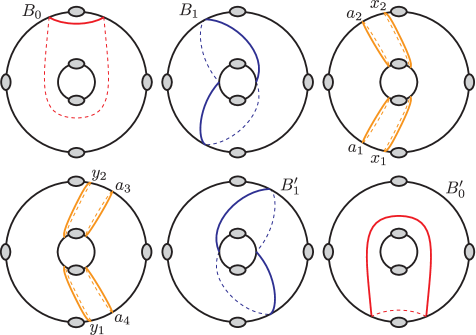
Refer to caption
Figure 6. The curve configuration for our 666–holed torus relation.

A lift of the 666–holed torus relation: Here we pause our construction to capture a lift of the relation (5) in Mod(Σ16)ModsuperscriptsubscriptΣ16\operatorname{Mod}(\Sigma_{1}^{6}) to Mod(Σ1,16)ModsuperscriptsubscriptΣ116\operatorname{Mod}(\Sigma_{1,1}^{6}). This lift will involve a non-trivial point-pushing map, and thus it will not yield an honest section, but we will plug this information in later to describe a pseudosection for the penultimate signature zero genus–999 Lefschetz fibration.

Consider the lower half of the 666–holed torus Σ16superscriptsubscriptΣ16\Sigma_{1}^{6} and glue a 222–holed disk to the boundary component d6subscript𝑑6d_{6} so that the entire surface becomes Σ17superscriptsubscriptΣ17\Sigma_{1}^{7}, as illustrated on the left in Figure 7(a). Notice that the curves a1,x1,d6,d6′′subscript𝑎1subscript𝑥1superscriptsubscript𝑑6superscriptsubscript𝑑6′′a_{1},x_{1},d_{6}^{\prime},d_{6}^{\prime\prime} cobound a Σ04superscriptsubscriptΣ04\Sigma_{0}^{4}, so this is set up for a lantern substitution. We further add a disk with a marked point along the new boundary component d6′′superscriptsubscript𝑑6′′d_{6}^{\prime\prime}, which results in the surface Σ1,16superscriptsubscriptΣ116\Sigma_{1,1}^{6}. Now the curves d6subscript𝑑6d_{6}, x1superscriptsubscript𝑥1x_{1}^{\prime}, a1superscriptsubscript𝑎1a_{1}^{\prime} and d6′′superscriptsubscript𝑑6′′d_{6}^{\prime\prime}, as shown on the right in Figure 7(a), make up the configuration of a lantern relation, though this relation is reduced to

t\scaletod69ptt\scaletox19ptt\scaletoa19pt=t\scaletod69ptt\scaletox19ptt\scaletoa19ptsubscript𝑡\scaletosubscript𝑑69𝑝𝑡subscript𝑡\scaletosuperscriptsubscript𝑥19𝑝𝑡subscript𝑡\scaletosuperscriptsubscript𝑎19𝑝𝑡subscript𝑡\scaletosuperscriptsubscript𝑑69𝑝𝑡subscript𝑡\scaletosubscript𝑥19𝑝𝑡subscript𝑡\scaletosubscript𝑎19𝑝𝑡\displaystyle t_{\scaleto{\mathstrut d_{6}}{9pt}}t_{\scaleto{\mathstrut x_{1}^{\prime}}{9pt}}t_{\scaleto{\mathstrut a_{1}^{\prime}}{9pt}}=t_{\scaleto{\mathstrut d_{6}^{\prime}}{9pt}}t_{\scaleto{\mathstrut x_{1}}{9pt}}t_{\scaleto{\mathstrut a_{1}}{9pt}}

for the Dehn twist along d6′′superscriptsubscript𝑑6′′d_{6}^{\prime\prime} is trivial in Mod(Σ1,16)ModsuperscriptsubscriptΣ116\operatorname{Mod}(\Sigma_{1,1}^{6}). We substitute this relation to the 666–holed torus relation (5) as

t\scaletoδ19ptt\scaletoδ29ptt\scaletoδ39ptt\scaletoδ49ptt\scaletod59ptt\scaletod69ptsubscript𝑡\scaletosubscript𝛿19𝑝𝑡subscript𝑡\scaletosubscript𝛿29𝑝𝑡subscript𝑡\scaletosubscript𝛿39𝑝𝑡subscript𝑡\scaletosubscript𝛿49𝑝𝑡subscript𝑡\scaletosubscript𝑑59𝑝𝑡subscript𝑡\scaletosubscript𝑑69𝑝𝑡\displaystyle t_{\scaleto{\mathstrut\delta_{1}}{9pt}}t_{\scaleto{\mathstrut\delta_{2}}{9pt}}t_{\scaleto{\mathstrut\delta_{3}}{9pt}}t_{\scaleto{\mathstrut\delta_{4}}{9pt}}t_{\scaleto{\mathstrut d_{5}}{9pt}}t_{\scaleto{\mathstrut d_{6}}{9pt}} =t\scaletoB09ptt\scaletoB19ptt\scaletoa19ptt\scaletoa29ptt\scaletox19ptt\scaletox29ptt\scaletoa19pt1t\scaletox19pt1t\scaletod69pt1t\scaletod69ptt\scaletox19ptt\scaletoa19ptt\scaletoy19ptt\scaletoy29ptt\scaletoa39ptt\scaletoa49ptt\scaletoB19ptt\scaletoB09pt.absentsubscript𝑡\scaletosubscript𝐵09𝑝𝑡subscript𝑡\scaletosubscript𝐵19𝑝𝑡subscript𝑡\scaletosubscript𝑎19𝑝𝑡subscript𝑡\scaletosubscript𝑎29𝑝𝑡subscript𝑡\scaletosubscript𝑥19𝑝𝑡subscript𝑡\scaletosubscript𝑥29𝑝𝑡superscriptsubscript𝑡\scaletosubscript𝑎19𝑝𝑡1superscriptsubscript𝑡\scaletosubscript𝑥19𝑝𝑡1superscriptsubscript𝑡\scaletosuperscriptsubscript𝑑69𝑝𝑡1subscript𝑡\scaletosubscript𝑑69𝑝𝑡subscript𝑡\scaletosuperscriptsubscript𝑥19𝑝𝑡subscript𝑡\scaletosuperscriptsubscript𝑎19𝑝𝑡subscript𝑡\scaletosubscript𝑦19𝑝𝑡subscript𝑡\scaletosubscript𝑦29𝑝𝑡subscript𝑡\scaletosubscript𝑎39𝑝𝑡subscript𝑡\scaletosubscript𝑎49𝑝𝑡subscript𝑡\scaletosuperscriptsubscript𝐵19𝑝𝑡subscript𝑡\scaletosuperscriptsubscript𝐵09𝑝𝑡\displaystyle=t_{\scaleto{\mathstrut B_{0}}{9pt}}t_{\scaleto{\mathstrut B_{1}}{9pt}}\cdot t_{\scaleto{\mathstrut a_{1}}{9pt}}t_{\scaleto{\mathstrut a_{2}}{9pt}}t_{\scaleto{\mathstrut x_{1}}{9pt}}t_{\scaleto{\mathstrut x_{2}}{9pt}}\cdot t_{\scaleto{\mathstrut a_{1}}{9pt}}^{-1}t_{\scaleto{\mathstrut x_{1}}{9pt}}^{-1}t_{\scaleto{\mathstrut d_{6}^{\prime}}{9pt}}^{-1}t_{\scaleto{\mathstrut d_{6}}{9pt}}t_{\scaleto{\mathstrut x_{1}^{\prime}}{9pt}}t_{\scaleto{\mathstrut a_{1}^{\prime}}{9pt}}\cdot t_{\scaleto{\mathstrut y_{1}}{9pt}}t_{\scaleto{\mathstrut y_{2}}{9pt}}t_{\scaleto{\mathstrut a_{3}}{9pt}}t_{\scaleto{\mathstrut a_{4}}{9pt}}\cdot t_{\scaleto{\mathstrut B_{1}^{\prime}}{9pt}}t_{\scaleto{\mathstrut B_{0}^{\prime}}{9pt}}.

By commutativity and cancellation, we obtain

t\scaletoδ19ptt\scaletoδ29ptt\scaletoδ39ptt\scaletoδ49ptt\scaletod59ptt\scaletod69ptsubscript𝑡\scaletosubscript𝛿19𝑝𝑡subscript𝑡\scaletosubscript𝛿29𝑝𝑡subscript𝑡\scaletosubscript𝛿39𝑝𝑡subscript𝑡\scaletosubscript𝛿49𝑝𝑡subscript𝑡\scaletosubscript𝑑59𝑝𝑡subscript𝑡\scaletosuperscriptsubscript𝑑69𝑝𝑡\displaystyle t_{\scaleto{\mathstrut\delta_{1}}{9pt}}t_{\scaleto{\mathstrut\delta_{2}}{9pt}}t_{\scaleto{\mathstrut\delta_{3}}{9pt}}t_{\scaleto{\mathstrut\delta_{4}}{9pt}}t_{\scaleto{\mathstrut d_{5}}{9pt}}t_{\scaleto{\mathstrut d_{6}^{\prime}}{9pt}} =t\scaletoB09ptt\scaletoB19ptt\scaletoa29ptt\scaletox29ptt\scaletox19ptt\scaletoa19ptt\scaletoy19ptt\scaletoy29ptt\scaletoa39ptt\scaletoa49ptt\scaletoB19ptt\scaletoB09pt.absentsubscript𝑡\scaletosubscript𝐵09𝑝𝑡subscript𝑡\scaletosubscript𝐵19𝑝𝑡subscript𝑡\scaletosubscript𝑎29𝑝𝑡subscript𝑡\scaletosubscript𝑥29𝑝𝑡subscript𝑡\scaletosuperscriptsubscript𝑥19𝑝𝑡subscript𝑡\scaletosuperscriptsubscript𝑎19𝑝𝑡subscript𝑡\scaletosubscript𝑦19𝑝𝑡subscript𝑡\scaletosubscript𝑦29𝑝𝑡subscript𝑡\scaletosubscript𝑎39𝑝𝑡subscript𝑡\scaletosubscript𝑎49𝑝𝑡subscript𝑡\scaletosuperscriptsubscript𝐵19𝑝𝑡subscript𝑡\scaletosuperscriptsubscript𝐵09𝑝𝑡\displaystyle=t_{\scaleto{\mathstrut B_{0}}{9pt}}t_{\scaleto{\mathstrut B_{1}}{9pt}}\cdot t_{\scaleto{\mathstrut a_{2}}{9pt}}t_{\scaleto{\mathstrut x_{2}}{9pt}}\cdot t_{\scaleto{\mathstrut x_{1}^{\prime}}{9pt}}t_{\scaleto{\mathstrut a_{1}^{\prime}}{9pt}}\cdot t_{\scaleto{\mathstrut y_{1}}{9pt}}t_{\scaleto{\mathstrut y_{2}}{9pt}}t_{\scaleto{\mathstrut a_{3}}{9pt}}t_{\scaleto{\mathstrut a_{4}}{9pt}}\cdot t_{\scaleto{\mathstrut B_{1}^{\prime}}{9pt}}t_{\scaleto{\mathstrut B_{0}^{\prime}}{9pt}}.

We then introduce canceling pairs t\scaletoa19ptt\scaletoa19pt1subscript𝑡\scaletosubscript𝑎19𝑝𝑡superscriptsubscript𝑡\scaletosubscript𝑎19𝑝𝑡1t_{\scaleto{\mathstrut a_{1}}{9pt}}t_{\scaleto{\mathstrut a_{1}}{9pt}}^{-1} and t\scaletoy19pt1t\scaletoy19ptsuperscriptsubscript𝑡\scaletosuperscriptsubscript𝑦19𝑝𝑡1subscript𝑡\scaletosuperscriptsubscript𝑦19𝑝𝑡t_{\scaleto{\mathstrut y_{1}^{\prime}}{9pt}}^{-1}t_{\scaleto{\mathstrut y_{1}^{\prime}}{9pt}} where the curve y1superscriptsubscript𝑦1y_{1}^{\prime} is as in Figure 7(b).

t\scaletoδ19ptt\scaletoδ29ptt\scaletoδ39ptt\scaletoδ49ptt\scaletod59ptt\scaletod69ptsubscript𝑡\scaletosubscript𝛿19𝑝𝑡subscript𝑡\scaletosubscript𝛿29𝑝𝑡subscript𝑡\scaletosubscript𝛿39𝑝𝑡subscript𝑡\scaletosubscript𝛿49𝑝𝑡subscript𝑡\scaletosubscript𝑑59𝑝𝑡subscript𝑡\scaletosuperscriptsubscript𝑑69𝑝𝑡\displaystyle t_{\scaleto{\mathstrut\delta_{1}}{9pt}}t_{\scaleto{\mathstrut\delta_{2}}{9pt}}t_{\scaleto{\mathstrut\delta_{3}}{9pt}}t_{\scaleto{\mathstrut\delta_{4}}{9pt}}t_{\scaleto{\mathstrut d_{5}}{9pt}}t_{\scaleto{\mathstrut d_{6}^{\prime}}{9pt}} =t\scaletoB09ptt\scaletoB19ptt\scaletoa29ptt\scaletox29ptt\scaletoa19ptt\scaletoa19pt1t\scaletox19ptt\scaletoa19ptt\scaletoy19pt1t\scaletoy19ptt\scaletoy19ptt\scaletoy29ptt\scaletoa39ptt\scaletoa49ptt\scaletoB19ptt\scaletoB09ptabsentsubscript𝑡\scaletosubscript𝐵09𝑝𝑡subscript𝑡\scaletosubscript𝐵19𝑝𝑡subscript𝑡\scaletosubscript𝑎29𝑝𝑡subscript𝑡\scaletosubscript𝑥29𝑝𝑡subscript𝑡\scaletosubscript𝑎19𝑝𝑡superscriptsubscript𝑡\scaletosubscript𝑎19𝑝𝑡1subscript𝑡\scaletosuperscriptsubscript𝑥19𝑝𝑡subscript𝑡\scaletosuperscriptsubscript𝑎19𝑝𝑡superscriptsubscript𝑡\scaletosuperscriptsubscript𝑦19𝑝𝑡1subscript𝑡\scaletosuperscriptsubscript𝑦19𝑝𝑡subscript𝑡\scaletosubscript𝑦19𝑝𝑡subscript𝑡\scaletosubscript𝑦29𝑝𝑡subscript𝑡\scaletosubscript𝑎39𝑝𝑡subscript𝑡\scaletosubscript𝑎49𝑝𝑡subscript𝑡\scaletosuperscriptsubscript𝐵19𝑝𝑡subscript𝑡\scaletosuperscriptsubscript𝐵09𝑝𝑡\displaystyle=t_{\scaleto{\mathstrut B_{0}}{9pt}}t_{\scaleto{\mathstrut B_{1}}{9pt}}\cdot t_{\scaleto{\mathstrut a_{2}}{9pt}}t_{\scaleto{\mathstrut x_{2}}{9pt}}\cdot t_{\scaleto{\mathstrut a_{1}}{9pt}}t_{\scaleto{\mathstrut a_{1}}{9pt}}^{-1}\cdot t_{\scaleto{\mathstrut x_{1}^{\prime}}{9pt}}t_{\scaleto{\mathstrut a_{1}^{\prime}}{9pt}}\cdot t_{\scaleto{\mathstrut y_{1}^{\prime}}{9pt}}^{-1}t_{\scaleto{\mathstrut y_{1}^{\prime}}{9pt}}\cdot t_{\scaleto{\mathstrut y_{1}}{9pt}}t_{\scaleto{\mathstrut y_{2}}{9pt}}t_{\scaleto{\mathstrut a_{3}}{9pt}}t_{\scaleto{\mathstrut a_{4}}{9pt}}\cdot t_{\scaleto{\mathstrut B_{1}^{\prime}}{9pt}}t_{\scaleto{\mathstrut B_{0}^{\prime}}{9pt}}
=t\scaletoB09ptt\scaletoB19ptt\scaletoa29ptt\scaletox29ptt\scaletoa19ptt\scaletox19ptt\scaletoa19pt1t\scaletoa19ptt\scaletoy19pt1t\scaletoy19ptt\scaletoy19ptt\scaletoy29ptt\scaletoa39ptt\scaletoa49ptt\scaletoB19ptt\scaletoB09pt.absentsubscript𝑡\scaletosubscript𝐵09𝑝𝑡subscript𝑡\scaletosubscript𝐵19𝑝𝑡subscript𝑡\scaletosubscript𝑎29𝑝𝑡subscript𝑡\scaletosubscript𝑥29𝑝𝑡subscript𝑡\scaletosubscript𝑎19𝑝𝑡subscript𝑡\scaletosuperscriptsubscript𝑥19𝑝𝑡superscriptsubscript𝑡\scaletosubscript𝑎19𝑝𝑡1subscript𝑡\scaletosuperscriptsubscript𝑎19𝑝𝑡superscriptsubscript𝑡\scaletosuperscriptsubscript𝑦19𝑝𝑡1subscript𝑡\scaletosubscript𝑦19𝑝𝑡subscript𝑡\scaletosuperscriptsubscript𝑦19𝑝𝑡subscript𝑡\scaletosubscript𝑦29𝑝𝑡subscript𝑡\scaletosubscript𝑎39𝑝𝑡subscript𝑡\scaletosubscript𝑎49𝑝𝑡subscript𝑡\scaletosuperscriptsubscript𝐵19𝑝𝑡subscript𝑡\scaletosuperscriptsubscript𝐵09𝑝𝑡\displaystyle=t_{\scaleto{\mathstrut B_{0}}{9pt}}t_{\scaleto{\mathstrut B_{1}}{9pt}}\cdot t_{\scaleto{\mathstrut a_{2}}{9pt}}t_{\scaleto{\mathstrut x_{2}}{9pt}}t_{\scaleto{\mathstrut a_{1}}{9pt}}t_{\scaleto{\mathstrut x_{1}^{\prime}}{9pt}}\cdot t_{\scaleto{\mathstrut a_{1}}{9pt}}^{-1}t_{\scaleto{\mathstrut a_{1}^{\prime}}{9pt}}\cdot t_{\scaleto{\mathstrut y_{1}^{\prime}}{9pt}}^{-1}t_{\scaleto{\mathstrut y_{1}}{9pt}}\cdot t_{\scaleto{\mathstrut y_{1}^{\prime}}{9pt}}t_{\scaleto{\mathstrut y_{2}}{9pt}}t_{\scaleto{\mathstrut a_{3}}{9pt}}t_{\scaleto{\mathstrut a_{4}}{9pt}}\cdot t_{\scaleto{\mathstrut B_{1}^{\prime}}{9pt}}t_{\scaleto{\mathstrut B_{0}^{\prime}}{9pt}}.

Observe that a1,a1subscript𝑎1superscriptsubscript𝑎1a_{1},a_{1}^{\prime} are parallel curves between which the marked point lies, so are y1,y1subscript𝑦1superscriptsubscript𝑦1y_{1},y_{1}^{\prime}. Therefore, the factors t\scaletoa19pt1t\scaletoa19ptsuperscriptsubscript𝑡\scaletosubscript𝑎19𝑝𝑡1subscript𝑡\scaletosuperscriptsubscript𝑎19𝑝𝑡t_{\scaleto{\mathstrut a_{1}}{9pt}}^{-1}t_{\scaleto{\mathstrut a_{1}^{\prime}}{9pt}} and t\scaletoy19pt1t\scaletoy19ptsuperscriptsubscript𝑡\scaletosuperscriptsubscript𝑦19𝑝𝑡1subscript𝑡\scaletosubscript𝑦19𝑝𝑡t_{\scaleto{\mathstrut y_{1}^{\prime}}{9pt}}^{-1}t_{\scaleto{\mathstrut y_{1}}{9pt}} can be viewed as, respectively, the point-pushing maps 𝒫β1subscript𝒫subscript𝛽1\mathcal{P}_{\vec{\beta}_{1}} and 𝒫β2subscript𝒫subscript𝛽2\mathcal{P}_{\vec{\beta}_{2}} along the oriented loops β1subscript𝛽1\vec{\beta}_{1} and β2subscript𝛽2\vec{\beta}_{2} in Figure 7(c). The product 𝒫β1𝒫β2subscript𝒫subscript𝛽1subscript𝒫subscript𝛽2\mathcal{P}_{\vec{\beta}_{1}}\mathcal{P}_{\vec{\beta}_{2}}, in turn, can be seen as the single point-pushing map 𝒫α0subscript𝒫subscript𝛼0\mathcal{P}_{\vec{\alpha}_{0}} along α0subscript𝛼0\vec{\alpha}_{0}, which is homotopic to the concatenation of β2subscript𝛽2\vec{\beta}_{2} and β1subscript𝛽1\vec{\beta}_{1}. The oriented loop α0subscript𝛼0\vec{\alpha}_{0} is shown in Figure 7(c).

Refer to caption
(a) Left: Adding a 222–holed disk to the 666–holed torus. Right: Capping off with a disk with a marked point, and getting a reduced lantern configuration.
Refer to caption
(b) Introducing canceling pairs about a1subscript𝑎1a_{1} and y1superscriptsubscript𝑦1y_{1}^{\prime}.
Refer to caption
(c) The oriented loops β1subscript𝛽1\vec{\beta}_{1}, β2subscript𝛽2\vec{\beta}_{2}, and α0subscript𝛼0\vec{\alpha}_{0} of the point-pushing maps.
Figure 7. Finding a pseudosection of the 666–holed torus relation.

In summary, we have

t\scaletoδ19ptt\scaletoδ29ptt\scaletoδ39ptt\scaletoδ49ptt\scaletod59ptt\scaletod69ptsubscript𝑡\scaletosubscript𝛿19𝑝𝑡subscript𝑡\scaletosubscript𝛿29𝑝𝑡subscript𝑡\scaletosubscript𝛿39𝑝𝑡subscript𝑡\scaletosubscript𝛿49𝑝𝑡subscript𝑡\scaletosubscript𝑑59𝑝𝑡subscript𝑡\scaletosuperscriptsubscript𝑑69𝑝𝑡\displaystyle t_{\scaleto{\mathstrut\delta_{1}}{9pt}}t_{\scaleto{\mathstrut\delta_{2}}{9pt}}t_{\scaleto{\mathstrut\delta_{3}}{9pt}}t_{\scaleto{\mathstrut\delta_{4}}{9pt}}t_{\scaleto{\mathstrut d_{5}}{9pt}}t_{\scaleto{\mathstrut d_{6}^{\prime}}{9pt}} =t\scaletoB09ptt\scaletoB19ptt\scaletoa29ptt\scaletox29ptt\scaletoa19ptt\scaletox19ptt\scaletoa19pt1t\scaletoa19ptt\scaletoy19pt1t\scaletoy19ptt\scaletoy19ptt\scaletoy29ptt\scaletoa39ptt\scaletoa49ptt\scaletoB19ptt\scaletoB09ptabsentsubscript𝑡\scaletosubscript𝐵09𝑝𝑡subscript𝑡\scaletosubscript𝐵19𝑝𝑡subscript𝑡\scaletosubscript𝑎29𝑝𝑡subscript𝑡\scaletosubscript𝑥29𝑝𝑡subscript𝑡\scaletosubscript𝑎19𝑝𝑡subscript𝑡\scaletosuperscriptsubscript𝑥19𝑝𝑡superscriptsubscript𝑡\scaletosubscript𝑎19𝑝𝑡1subscript𝑡\scaletosuperscriptsubscript𝑎19𝑝𝑡superscriptsubscript𝑡\scaletosuperscriptsubscript𝑦19𝑝𝑡1subscript𝑡\scaletosubscript𝑦19𝑝𝑡subscript𝑡\scaletosuperscriptsubscript𝑦19𝑝𝑡subscript𝑡\scaletosubscript𝑦29𝑝𝑡subscript𝑡\scaletosubscript𝑎39𝑝𝑡subscript𝑡\scaletosubscript𝑎49𝑝𝑡subscript𝑡\scaletosuperscriptsubscript𝐵19𝑝𝑡subscript𝑡\scaletosuperscriptsubscript𝐵09𝑝𝑡\displaystyle=t_{\scaleto{\mathstrut B_{0}}{9pt}}t_{\scaleto{\mathstrut B_{1}}{9pt}}\cdot t_{\scaleto{\mathstrut a_{2}}{9pt}}t_{\scaleto{\mathstrut x_{2}}{9pt}}t_{\scaleto{\mathstrut a_{1}}{9pt}}t_{\scaleto{\mathstrut x_{1}^{\prime}}{9pt}}\cdot t_{\scaleto{\mathstrut a_{1}}{9pt}}^{-1}t_{\scaleto{\mathstrut a_{1}^{\prime}}{9pt}}\cdot t_{\scaleto{\mathstrut y_{1}^{\prime}}{9pt}}^{-1}t_{\scaleto{\mathstrut y_{1}}{9pt}}\cdot t_{\scaleto{\mathstrut y_{1}^{\prime}}{9pt}}t_{\scaleto{\mathstrut y_{2}}{9pt}}t_{\scaleto{\mathstrut a_{3}}{9pt}}t_{\scaleto{\mathstrut a_{4}}{9pt}}\cdot t_{\scaleto{\mathstrut B_{1}^{\prime}}{9pt}}t_{\scaleto{\mathstrut B_{0}^{\prime}}{9pt}}
=t\scaletoB09ptt\scaletoB19ptt\scaletoa29ptt\scaletox29ptt\scaletoa19ptt\scaletox19pt𝒫β1𝒫β2t\scaletoy19ptt\scaletoy29ptt\scaletoa39ptt\scaletoa49ptt\scaletoB19ptt\scaletoB09ptabsentsubscript𝑡\scaletosubscript𝐵09𝑝𝑡subscript𝑡\scaletosubscript𝐵19𝑝𝑡subscript𝑡\scaletosubscript𝑎29𝑝𝑡subscript𝑡\scaletosubscript𝑥29𝑝𝑡subscript𝑡\scaletosubscript𝑎19𝑝𝑡subscript𝑡\scaletosuperscriptsubscript𝑥19𝑝𝑡subscript𝒫subscript𝛽1subscript𝒫subscript𝛽2subscript𝑡\scaletosuperscriptsubscript𝑦19𝑝𝑡subscript𝑡\scaletosubscript𝑦29𝑝𝑡subscript𝑡\scaletosubscript𝑎39𝑝𝑡subscript𝑡\scaletosubscript𝑎49𝑝𝑡subscript𝑡\scaletosuperscriptsubscript𝐵19𝑝𝑡subscript𝑡\scaletosuperscriptsubscript𝐵09𝑝𝑡\displaystyle=t_{\scaleto{\mathstrut B_{0}}{9pt}}t_{\scaleto{\mathstrut B_{1}}{9pt}}\cdot t_{\scaleto{\mathstrut a_{2}}{9pt}}t_{\scaleto{\mathstrut x_{2}}{9pt}}t_{\scaleto{\mathstrut a_{1}}{9pt}}t_{\scaleto{\mathstrut x_{1}^{\prime}}{9pt}}\cdot\mathcal{P}_{\vec{\beta}_{1}}\cdot\mathcal{P}_{\vec{\beta}_{2}}\cdot t_{\scaleto{\mathstrut y_{1}^{\prime}}{9pt}}t_{\scaleto{\mathstrut y_{2}}{9pt}}t_{\scaleto{\mathstrut a_{3}}{9pt}}t_{\scaleto{\mathstrut a_{4}}{9pt}}\cdot t_{\scaleto{\mathstrut B_{1}^{\prime}}{9pt}}t_{\scaleto{\mathstrut B_{0}^{\prime}}{9pt}}
=t\scaletoB09ptt\scaletoB19ptt\scaletoa29ptt\scaletox29ptt\scaletoa19ptt\scaletox19pt𝒫α0t\scaletoy19ptt\scaletoy29ptt\scaletoa39ptt\scaletoa49ptt\scaletoB19ptt\scaletoB09pt.absentsubscript𝑡\scaletosubscript𝐵09𝑝𝑡subscript𝑡\scaletosubscript𝐵19𝑝𝑡subscript𝑡\scaletosubscript𝑎29𝑝𝑡subscript𝑡\scaletosubscript𝑥29𝑝𝑡subscript𝑡\scaletosubscript𝑎19𝑝𝑡subscript𝑡\scaletosuperscriptsubscript𝑥19𝑝𝑡subscript𝒫subscript𝛼0subscript𝑡\scaletosuperscriptsubscript𝑦19𝑝𝑡subscript𝑡\scaletosubscript𝑦29𝑝𝑡subscript𝑡\scaletosubscript𝑎39𝑝𝑡subscript𝑡\scaletosubscript𝑎49𝑝𝑡subscript𝑡\scaletosuperscriptsubscript𝐵19𝑝𝑡subscript𝑡\scaletosuperscriptsubscript𝐵09𝑝𝑡\displaystyle=t_{\scaleto{\mathstrut B_{0}}{9pt}}t_{\scaleto{\mathstrut B_{1}}{9pt}}\cdot t_{\scaleto{\mathstrut a_{2}}{9pt}}t_{\scaleto{\mathstrut x_{2}}{9pt}}t_{\scaleto{\mathstrut a_{1}}{9pt}}t_{\scaleto{\mathstrut x_{1}^{\prime}}{9pt}}\cdot\mathcal{P}_{\vec{\alpha}_{0}}\cdot t_{\scaleto{\mathstrut y_{1}^{\prime}}{9pt}}t_{\scaleto{\mathstrut y_{2}}{9pt}}t_{\scaleto{\mathstrut a_{3}}{9pt}}t_{\scaleto{\mathstrut a_{4}}{9pt}}\cdot t_{\scaleto{\mathstrut B_{1}^{\prime}}{9pt}}t_{\scaleto{\mathstrut B_{0}^{\prime}}{9pt}}.

Finally, by dropping the prime symbol from d6superscriptsubscript𝑑6d_{6}^{\prime}, x1superscriptsubscript𝑥1x_{1}^{\prime}, y1superscriptsubscript𝑦1y_{1}^{\prime} (which should cause no confusion with the previous notation) we rewrite this relation in Mod(Σ1,16)ModsuperscriptsubscriptΣ116\operatorname{Mod}(\Sigma_{1,1}^{6}) as:

(6) t\scaletoδ19ptt\scaletoδ29ptt\scaletoδ39ptt\scaletoδ49ptt\scaletod59ptt\scaletod69ptsubscript𝑡\scaletosubscript𝛿19𝑝𝑡subscript𝑡\scaletosubscript𝛿29𝑝𝑡subscript𝑡\scaletosubscript𝛿39𝑝𝑡subscript𝑡\scaletosubscript𝛿49𝑝𝑡subscript𝑡\scaletosubscript𝑑59𝑝𝑡subscript𝑡\scaletosubscript𝑑69𝑝𝑡\displaystyle t_{\scaleto{\mathstrut\delta_{1}}{9pt}}t_{\scaleto{\mathstrut\delta_{2}}{9pt}}t_{\scaleto{\mathstrut\delta_{3}}{9pt}}t_{\scaleto{\mathstrut\delta_{4}}{9pt}}t_{\scaleto{\mathstrut d_{5}}{9pt}}t_{\scaleto{\mathstrut d_{6}}{9pt}} =t\scaletoB09ptt\scaletoB19ptt\scaletoa19ptt\scaletoa29ptt\scaletox19ptt\scaletox29pt𝒫α0t\scaletoy19ptt\scaletoy29ptt\scaletoa39ptt\scaletoa49ptt\scaletoB19ptt\scaletoB09pt,absentsubscript𝑡\scaletosubscript𝐵09𝑝𝑡subscript𝑡\scaletosubscript𝐵19𝑝𝑡subscript𝑡\scaletosubscript𝑎19𝑝𝑡subscript𝑡\scaletosubscript𝑎29𝑝𝑡subscript𝑡\scaletosubscript𝑥19𝑝𝑡subscript𝑡\scaletosubscript𝑥29𝑝𝑡subscript𝒫subscript𝛼0subscript𝑡\scaletosubscript𝑦19𝑝𝑡subscript𝑡\scaletosubscript𝑦29𝑝𝑡subscript𝑡\scaletosubscript𝑎39𝑝𝑡subscript𝑡\scaletosubscript𝑎49𝑝𝑡subscript𝑡\scaletosuperscriptsubscript𝐵19𝑝𝑡subscript𝑡\scaletosuperscriptsubscript𝐵09𝑝𝑡\displaystyle=t_{\scaleto{\mathstrut B_{0}}{9pt}}t_{\scaleto{\mathstrut B_{1}}{9pt}}\cdot t_{\scaleto{\mathstrut a_{1}}{9pt}}t_{\scaleto{\mathstrut a_{2}}{9pt}}t_{\scaleto{\mathstrut x_{1}}{9pt}}t_{\scaleto{\mathstrut x_{2}}{9pt}}\cdot\mathcal{P}_{\vec{\alpha}_{0}}\cdot t_{\scaleto{\mathstrut y_{1}}{9pt}}t_{\scaleto{\mathstrut y_{2}}{9pt}}t_{\scaleto{\mathstrut a_{3}}{9pt}}t_{\scaleto{\mathstrut a_{4}}{9pt}}\cdot t_{\scaleto{\mathstrut B_{1}^{\prime}}{9pt}}t_{\scaleto{\mathstrut B_{0}^{\prime}}{9pt}},

where the curves are as illustrated in Figure 8. This is our lift of the 666–holed torus relation (5).

Refer to caption
Figure 8. The 666–holed torus relation with a marked point.

It happens that the oriented loop α0subscript𝛼0\vec{\alpha}_{0} of the point-pushing map in the lift encircles one of the boundary components without intersecting any of the Dehn twist curves. This will make it easier to describe lifts in later steps of our construction to follow.

A genus–222 pencil: We now construct the genus–222 Lefschetz pencil that will become one of our main building blocks. Take the boundary components d5subscript𝑑5d_{5}, d6subscript𝑑6d_{6} of the 666–holed torus Σ1,16superscriptsubscriptΣ116\Sigma_{1,1}^{6} in the previous step and connect them by a tube as shown in Figure 9(a). This gives a Σ2,14superscriptsubscriptΣ214\Sigma_{2,1}^{4}, a genus–222 surface with four boundary components and a marked point. The curves d5subscript𝑑5d_{5} and d6subscript𝑑6d_{6} become identical, so we denote both by d𝑑d.

Refer to caption
(a) The embedding of Σ1,16superscriptsubscriptΣ116\Sigma_{1,1}^{6} into Σ2,14superscriptsubscriptΣ214\Sigma_{2,1}^{4}.
Refer to caption
(b) Two configurations of lantern curves in Σ2,14superscriptsubscriptΣ214\Sigma_{2,1}^{4}.
Refer to caption
(c) Rearranging the boundary components δ3subscript𝛿3\delta_{3} and δ4subscript𝛿4\delta_{4}. On the right, δ4subscript𝛿4\delta_{4} is on the front and δ3subscript𝛿3\delta_{3} is on the back of the surface.
Figure 9. Construction of a genus–222 pencil.
Refer to caption
Figure 10. Vanishing cycles of a genus–222 pencil. Notice that B0,B0subscript𝐵0superscriptsubscript𝐵0B_{0},B_{0}^{\prime} is a bounding pair and the two separating curves C𝐶C, Csuperscript𝐶C^{\prime} are disjoint.

Now for the quadruples of curves a1,a2,x1,x2,dsubscript𝑎1subscript𝑎2subscript𝑥1subscript𝑥2𝑑a_{1},a_{2},x_{1},x_{2},d and y1,y2,a3,a4,dsubscript𝑦1subscript𝑦2subscript𝑎3subscript𝑎4𝑑y_{1},y_{2},a_{3},a_{4},d each cobounding a Σ04superscriptsubscriptΣ04\Sigma_{0}^{4} as shown in Figure 9(b), we have the lantern relations

t\scaletod9ptt\scaletoB29ptt\scaletoC9ptsubscript𝑡\scaleto𝑑9𝑝𝑡subscript𝑡\scaletosubscript𝐵29𝑝𝑡subscript𝑡\scaleto𝐶9𝑝𝑡\displaystyle t_{\scaleto{\mathstrut d}{9pt}}t_{\scaleto{\mathstrut B_{2}}{9pt}}t_{\scaleto{\mathstrut C}{9pt}} =t\scaletoa19ptt\scaletoa29ptt\scaletox19ptt\scaletox29pt,absentsubscript𝑡\scaletosubscript𝑎19𝑝𝑡subscript𝑡\scaletosubscript𝑎29𝑝𝑡subscript𝑡\scaletosubscript𝑥19𝑝𝑡subscript𝑡\scaletosubscript𝑥29𝑝𝑡\displaystyle=t_{\scaleto{\mathstrut a_{1}}{9pt}}t_{\scaleto{\mathstrut a_{2}}{9pt}}t_{\scaleto{\mathstrut x_{1}}{9pt}}t_{\scaleto{\mathstrut x_{2}}{9pt}},
t\scaletoC9ptt\scaletoB29ptt\scaletod9ptsubscript𝑡\scaletosuperscript𝐶9𝑝𝑡subscript𝑡\scaletosuperscriptsubscript𝐵29𝑝𝑡subscript𝑡\scaleto𝑑9𝑝𝑡\displaystyle t_{\scaleto{\mathstrut C^{\prime}}{9pt}}t_{\scaleto{\mathstrut B_{2}^{\prime}}{9pt}}t_{\scaleto{\mathstrut d}{9pt}} =t\scaletoy19ptt\scaletoy29ptt\scaletoa39ptt\scaletoa49pt,absentsubscript𝑡\scaletosubscript𝑦19𝑝𝑡subscript𝑡\scaletosubscript𝑦29𝑝𝑡subscript𝑡\scaletosubscript𝑎39𝑝𝑡subscript𝑡\scaletosubscript𝑎49𝑝𝑡\displaystyle=t_{\scaleto{\mathstrut y_{1}}{9pt}}t_{\scaleto{\mathstrut y_{2}}{9pt}}t_{\scaleto{\mathstrut a_{3}}{9pt}}t_{\scaleto{\mathstrut a_{4}}{9pt}},

where the curves B2,C,C,B2subscript𝐵2𝐶superscript𝐶superscriptsubscript𝐵2B_{2},C,C^{\prime},B_{2}^{\prime} are as in Figure 9(b). Combining the two with our 666–holed torus relation (6) yields

t\scaletoδ19ptt\scaletoδ29ptt\scaletoδ39ptt\scaletoδ49ptt\scaletod9ptt\scaletod9ptsubscript𝑡\scaletosubscript𝛿19𝑝𝑡subscript𝑡\scaletosubscript𝛿29𝑝𝑡subscript𝑡\scaletosubscript𝛿39𝑝𝑡subscript𝑡\scaletosubscript𝛿49𝑝𝑡subscript𝑡\scaleto𝑑9𝑝𝑡subscript𝑡\scaleto𝑑9𝑝𝑡\displaystyle t_{\scaleto{\mathstrut\delta_{1}}{9pt}}t_{\scaleto{\mathstrut\delta_{2}}{9pt}}t_{\scaleto{\mathstrut\delta_{3}}{9pt}}t_{\scaleto{\mathstrut\delta_{4}}{9pt}}t_{\scaleto{\mathstrut d}{9pt}}t_{\scaleto{\mathstrut d}{9pt}} =t\scaletoB09ptt\scaletoB19ptt\scaletoa19ptt\scaletoa29ptt\scaletox19ptt\scaletox29pt¯𝒫α0t\scaletoy19ptt\scaletoy29ptt\scaletoa39ptt\scaletoa49pt¯t\scaletoB19ptt\scaletoB09ptabsentsubscript𝑡\scaletosubscript𝐵09𝑝𝑡subscript𝑡\scaletosubscript𝐵19𝑝𝑡¯subscript𝑡\scaletosubscript𝑎19𝑝𝑡subscript𝑡\scaletosubscript𝑎29𝑝𝑡subscript𝑡\scaletosubscript𝑥19𝑝𝑡subscript𝑡\scaletosubscript𝑥29𝑝𝑡subscript𝒫subscript𝛼0¯subscript𝑡\scaletosubscript𝑦19𝑝𝑡subscript𝑡\scaletosubscript𝑦29𝑝𝑡subscript𝑡\scaletosubscript𝑎39𝑝𝑡subscript𝑡\scaletosubscript𝑎49𝑝𝑡subscript𝑡\scaletosuperscriptsubscript𝐵19𝑝𝑡subscript𝑡\scaletosuperscriptsubscript𝐵09𝑝𝑡\displaystyle=t_{\scaleto{\mathstrut B_{0}}{9pt}}t_{\scaleto{\mathstrut B_{1}}{9pt}}\cdot\underline{t_{\scaleto{\mathstrut a_{1}}{9pt}}t_{\scaleto{\mathstrut a_{2}}{9pt}}t_{\scaleto{\mathstrut x_{1}}{9pt}}t_{\scaleto{\mathstrut x_{2}}{9pt}}}\cdot\mathcal{P}_{\vec{\alpha}_{0}}\cdot\underline{t_{\scaleto{\mathstrut y_{1}}{9pt}}t_{\scaleto{\mathstrut y_{2}}{9pt}}t_{\scaleto{\mathstrut a_{3}}{9pt}}t_{\scaleto{\mathstrut a_{4}}{9pt}}}\cdot t_{\scaleto{\mathstrut B_{1}^{\prime}}{9pt}}t_{\scaleto{\mathstrut B_{0}^{\prime}}{9pt}}
=t\scaletoB09ptt\scaletoB19ptt\scaletod9ptt\scaletoB29ptt\scaletoC9pt𝒫α0t\scaletoC9ptt\scaletoB29ptt\scaletod9ptt\scaletoB19ptt\scaletoB09pt.absentsubscript𝑡\scaletosubscript𝐵09𝑝𝑡subscript𝑡\scaletosubscript𝐵19𝑝𝑡subscript𝑡\scaleto𝑑9𝑝𝑡subscript𝑡\scaletosubscript𝐵29𝑝𝑡subscript𝑡\scaleto𝐶9𝑝𝑡subscript𝒫subscript𝛼0subscript𝑡\scaletosuperscript𝐶9𝑝𝑡subscript𝑡\scaletosuperscriptsubscript𝐵29𝑝𝑡subscript𝑡\scaleto𝑑9𝑝𝑡subscript𝑡\scaletosuperscriptsubscript𝐵19𝑝𝑡subscript𝑡\scaletosuperscriptsubscript𝐵09𝑝𝑡\displaystyle=t_{\scaleto{\mathstrut B_{0}}{9pt}}t_{\scaleto{\mathstrut B_{1}}{9pt}}\cdot t_{\scaleto{\mathstrut d}{9pt}}t_{\scaleto{\mathstrut B_{2}}{9pt}}t_{\scaleto{\mathstrut C}{9pt}}\cdot\mathcal{P}_{\vec{\alpha}_{0}}\cdot t_{\scaleto{\mathstrut C^{\prime}}{9pt}}t_{\scaleto{\mathstrut B_{2}^{\prime}}{9pt}}t_{\scaleto{\mathstrut d}{9pt}}\cdot t_{\scaleto{\mathstrut B_{1}^{\prime}}{9pt}}t_{\scaleto{\mathstrut B_{0}^{\prime}}{9pt}}.

By canceling the t\scaletod9ptsubscript𝑡\scaleto𝑑9𝑝𝑡t_{\scaleto{\mathstrut d}{9pt}} factors we obtain the relation

(7) t\scaletoδ19ptt\scaletoδ29ptt\scaletoδ39ptt\scaletoδ49ptsubscript𝑡\scaletosubscript𝛿19𝑝𝑡subscript𝑡\scaletosubscript𝛿29𝑝𝑡subscript𝑡\scaletosubscript𝛿39𝑝𝑡subscript𝑡\scaletosubscript𝛿49𝑝𝑡\displaystyle t_{\scaleto{\mathstrut\delta_{1}}{9pt}}t_{\scaleto{\mathstrut\delta_{2}}{9pt}}t_{\scaleto{\mathstrut\delta_{3}}{9pt}}t_{\scaleto{\mathstrut\delta_{4}}{9pt}} =t\scaletoB09ptt\scaletoB19ptt\scaletoB29ptt\scaletoC9pt𝒫α0t\scaletoC9ptt\scaletoB29ptt\scaletoB19ptt\scaletoB09ptabsentsubscript𝑡\scaletosubscript𝐵09𝑝𝑡subscript𝑡\scaletosubscript𝐵19𝑝𝑡subscript𝑡\scaletosubscript𝐵29𝑝𝑡subscript𝑡\scaleto𝐶9𝑝𝑡subscript𝒫subscript𝛼0subscript𝑡\scaletosuperscript𝐶9𝑝𝑡subscript𝑡\scaletosuperscriptsubscript𝐵29𝑝𝑡subscript𝑡\scaletosuperscriptsubscript𝐵19𝑝𝑡subscript𝑡\scaletosuperscriptsubscript𝐵09𝑝𝑡\displaystyle=t_{\scaleto{\mathstrut B_{0}}{9pt}}t_{\scaleto{\mathstrut B_{1}}{9pt}}t_{\scaleto{\mathstrut B_{2}}{9pt}}t_{\scaleto{\mathstrut C}{9pt}}\cdot\mathcal{P}_{\vec{\alpha}_{0}}\cdot t_{\scaleto{\mathstrut C^{\prime}}{9pt}}t_{\scaleto{\mathstrut B_{2}^{\prime}}{9pt}}t_{\scaleto{\mathstrut B_{1}^{\prime}}{9pt}}t_{\scaleto{\mathstrut B_{0}^{\prime}}{9pt}}

in Mod(Σ2,14)ModsuperscriptsubscriptΣ214\operatorname{Mod}(\Sigma_{2,1}^{4}). Moreover, after pushing the boundary components δ3subscript𝛿3\delta_{3} and δ4subscript𝛿4\delta_{4} as indicated in Figure 9(c), we get a neater presentation of the Dehn twist curves as illustrated in Figure 10. Pairs of curves labeled with the same letters, but one decorated with a prime and one without it, are all symmetric under the obvious involution.

The relation (7) (after forgetting the marked point) is the monodromy factorization for our genus–222 Lefschetz pencil. Observe that in the monodromy factorization (7) the pair B0,B0subscript𝐵0superscriptsubscript𝐵0B_{0},B_{0}^{\prime} cobounds two copies of Σ14superscriptsubscriptΣ14\Sigma_{1}^{4} with the boundary components, and we also have two disjoint separating curves C𝐶C and Csuperscript𝐶C^{\prime}, each of which cobounds a copy of Σ12superscriptsubscriptΣ12\Sigma_{1}^{2} with a boundary component.

Let us compute the signature σ𝜎\sigma of the total space of this genus–222 pencil. As we noted earlier, the 666–holed torus relation (5) is derived by using a single 222–chain relation and five lantern relations. We have then used two more lantern relations to obtain the relation (7). (Here we forget the marked point and the relations we employed for finding the point-pushing map.) Since the 222–chain relation and the lantern relation contribute 77-7 and +11+1 to the signature, respectively, we compute the signature of the pencil as   σ=1(7)+7(+1)=0𝜎17710\sigma=1(-7)+7(+1)=0.

We can moreover describe an explicit spin structure on this pencil (which we will make use of in Section 5.1.) Let {α1,β1,α2,β2,δ1,δ2,δ3}subscript𝛼1subscript𝛽1subscript𝛼2subscript𝛽2subscript𝛿1subscript𝛿2subscript𝛿3\{\alpha_{1},\beta_{1},\alpha_{2},\beta_{2},\delta_{1},\delta_{2},\delta_{3}\} be a basis for H1(Σ24;2)subscript𝐻1superscriptsubscriptΣ24subscript2H_{1}(\Sigma_{2}^{4};\mathbb{Z}_{2}), given by the same labeled curves in Figure 11.

Refer to caption
Figure 11. A basis for H1(Σ24;2)subscript𝐻1superscriptsubscriptΣ24subscript2H_{1}(\Sigma_{2}^{4};\mathbb{Z}_{2}).

We can then compute the 2subscript2\mathbb{Z}_{2}–homology classes of the vanishing cycles as:

B0subscript𝐵0\displaystyle B_{0} =α1+α2+δ1+δ2+δ3;absentsubscript𝛼1subscript𝛼2subscript𝛿1subscript𝛿2subscript𝛿3\displaystyle=\alpha_{1}+\alpha_{2}+\delta_{1}+\delta_{2}+\delta_{3};
B1subscript𝐵1\displaystyle B_{1} =α1+β1+α2+β2+δ1+δ2+δ3;absentsubscript𝛼1subscript𝛽1subscript𝛼2subscript𝛽2subscript𝛿1subscript𝛿2subscript𝛿3\displaystyle=\alpha_{1}+\beta_{1}+\alpha_{2}+\beta_{2}+\delta_{1}+\delta_{2}+\delta_{3};
B2subscript𝐵2\displaystyle B_{2} =β1+β2+δ1+δ2+δ3;absentsubscript𝛽1subscript𝛽2subscript𝛿1subscript𝛿2subscript𝛿3\displaystyle=\beta_{1}+\beta_{2}+\delta_{1}+\delta_{2}+\delta_{3};
C𝐶\displaystyle C =δ1;absentsubscript𝛿1\displaystyle=\delta_{1};
Csuperscript𝐶\displaystyle C^{\prime} =δ2;absentsubscript𝛿2\displaystyle=\delta_{2};
B2superscriptsubscript𝐵2\displaystyle B_{2}^{\prime} =β1+β2+δ3;absentsubscript𝛽1subscript𝛽2subscript𝛿3\displaystyle=\beta_{1}+\beta_{2}+\delta_{3};
B1superscriptsubscript𝐵1\displaystyle B_{1}^{\prime} =α1+β1+α2+β2+δ3;absentsubscript𝛼1subscript𝛽1subscript𝛼2subscript𝛽2subscript𝛿3\displaystyle=\alpha_{1}+\beta_{1}+\alpha_{2}+\beta_{2}+\delta_{3};
B0superscriptsubscript𝐵0\displaystyle B_{0}^{\prime} =α1+α2+δ3.absentsubscript𝛼1subscript𝛼2subscript𝛿3\displaystyle=\alpha_{1}+\alpha_{2}+\delta_{3}.

If we now define a quadratic form q𝑞q on H1(Σ24;2)subscript𝐻1superscriptsubscriptΣ24subscript2H_{1}(\Sigma_{2}^{4};\mathbb{Z}_{2}) such that

(8) q(αi)=q(βi)=q(δj)=1 for all i=1,2 and j=1,,4,formulae-sequence𝑞subscript𝛼𝑖𝑞subscript𝛽𝑖𝑞subscript𝛿𝑗1 for all 𝑖12 and 𝑗14q(\alpha_{i})=q(\beta_{i})=q(\delta_{j})=1\text{ for all }i=1,2\text{ and }j=1,\ldots,4\,,

then it maps each vanishing cycle to 111, and by Theorem 1, we get a spin structure on the total space of the pencil.

Equipping the pencil with a Gompf-Thurston symplectic form, we get a symplectic 444–manifold. Then, observing that the fiber of the pencil violates the adjunction inequality, we conclude that the total space has to be a rational or a ruled surface. As it quickly follows from the above calculation, the rank of the 2subscript2\mathbb{Z}_{2}–homology of this 444–manifold is two, thus it should be the ruled surface T2×S2superscript𝑇2superscript𝑆2T^{2}\times S^{2}.

Remark 12.

There are other explicit monodromy factorizations for genus–222 pencils with four base points on the ruled surface T2×S2superscript𝑇2superscript𝑆2T^{2}\times S^{2}, which were obtained by the second author in [32] as lifts of Matsumoto’s well-known relation [42]. It is natural to ask whether the one we discovered here is Hurwitz equivalent to any of those, and we will show that it is indeed the case in Appendix A.

3.2. A signature zero genus–333 pencil

We will next describe a genus–333 pencil, the total space of which has signature zero and is spin, whereas its monodromy has four (in fact five) pairs of Dehn twists along certain bounding pairs.

We breed two copies of the genus–222 pencil constructed in the previous subsection to obtain the desired genus–333 pencil. The curves δ1,δ3,C3,C4subscript𝛿1subscript𝛿3subscript𝐶3subscript𝐶4\delta_{1},\delta_{3},C_{3},C_{4} on Σ3,24superscriptsubscriptΣ324\Sigma_{3,2}^{4} in Figure 12 cobound a subsurface diffeomorphic to Σ2,14superscriptsubscriptΣ214\Sigma_{2,1}^{4}. The same goes for the curves δ2,δ4,C1,C2subscript𝛿2subscript𝛿4subscript𝐶1subscript𝐶2\delta_{2},\delta_{4},C_{1},C_{2}. Thus, we can embed two copies of the relation (7) in Mod(Σ2,14)ModsuperscriptsubscriptΣ214\operatorname{Mod}(\Sigma_{2,1}^{4}) into Mod(Σ3,14)ModsuperscriptsubscriptΣ314\operatorname{Mod}(\Sigma_{3,1}^{4}) as

t\scaletoa9ptt\scaletox9ptt\scaletob9ptt\scaletoC19pt𝒫α1t\scaletoC29ptt\scaletod9ptt\scaletow9ptt\scaletoa9pt=t\scaletoδ19ptt\scaletoδ39ptt\scaletoC39ptt\scaletoC49pt,subscript𝑡\scaletosuperscript𝑎9𝑝𝑡subscript𝑡\scaleto𝑥9𝑝𝑡subscript𝑡\scaleto𝑏9𝑝𝑡subscript𝑡\scaletosubscript𝐶19𝑝𝑡subscript𝒫subscript𝛼1subscript𝑡\scaletosubscript𝐶29𝑝𝑡subscript𝑡\scaletosuperscript𝑑9𝑝𝑡subscript𝑡\scaleto𝑤9𝑝𝑡subscript𝑡\scaleto𝑎9𝑝𝑡subscript𝑡\scaletosubscript𝛿19𝑝𝑡subscript𝑡\scaletosubscript𝛿39𝑝𝑡subscript𝑡\scaletosubscript𝐶39𝑝𝑡subscript𝑡\scaletosubscript𝐶49𝑝𝑡\displaystyle t_{\scaleto{\mathstrut a^{\prime}}{9pt}}t_{\scaleto{\mathstrut x}{9pt}}t_{\scaleto{\mathstrut b}{9pt}}t_{\scaleto{\mathstrut C_{1}}{9pt}}\cdot\mathcal{P}_{\vec{\alpha}_{1}}\cdot t_{\scaleto{\mathstrut C_{2}}{9pt}}t_{\scaleto{\mathstrut d^{\prime}}{9pt}}t_{\scaleto{\mathstrut w}{9pt}}t_{\scaleto{\mathstrut a}{9pt}}=t_{\scaleto{\mathstrut\delta_{1}}{9pt}}t_{\scaleto{\mathstrut\delta_{3}}{9pt}}t_{\scaleto{\mathstrut C_{3}}{9pt}}t_{\scaleto{\mathstrut C_{4}}{9pt}},
t\scaletoc9ptt\scaletoz9ptt\scaletod9ptt\scaletoC39pt𝒫α2t\scaletoC49ptt\scaletob9ptt\scaletoy9ptt\scaletoc9pt=t\scaletoδ29ptt\scaletoδ49ptt\scaletoC19ptt\scaletoC29pt,subscript𝑡\scaletosuperscript𝑐9𝑝𝑡subscript𝑡\scaleto𝑧9𝑝𝑡subscript𝑡\scaleto𝑑9𝑝𝑡subscript𝑡\scaletosubscript𝐶39𝑝𝑡subscript𝒫subscript𝛼2subscript𝑡\scaletosubscript𝐶49𝑝𝑡subscript𝑡\scaletosuperscript𝑏9𝑝𝑡subscript𝑡\scaleto𝑦9𝑝𝑡subscript𝑡\scaleto𝑐9𝑝𝑡subscript𝑡\scaletosubscript𝛿29𝑝𝑡subscript𝑡\scaletosubscript𝛿49𝑝𝑡subscript𝑡\scaletosubscript𝐶19𝑝𝑡subscript𝑡\scaletosubscript𝐶29𝑝𝑡\displaystyle t_{\scaleto{\mathstrut c^{\prime}}{9pt}}t_{\scaleto{\mathstrut z}{9pt}}t_{\scaleto{\mathstrut d}{9pt}}t_{\scaleto{\mathstrut C_{3}}{9pt}}\cdot\mathcal{P}_{\vec{\alpha}_{2}}\cdot t_{\scaleto{\mathstrut C_{4}}{9pt}}t_{\scaleto{\mathstrut b^{\prime}}{9pt}}t_{\scaleto{\mathstrut y}{9pt}}t_{\scaleto{\mathstrut c}{9pt}}=t_{\scaleto{\mathstrut\delta_{2}}{9pt}}t_{\scaleto{\mathstrut\delta_{4}}{9pt}}t_{\scaleto{\mathstrut C_{1}}{9pt}}t_{\scaleto{\mathstrut C_{2}}{9pt}},

where the curves are as shown in Figure 13. Note that the second embedding is obtained by the first embedding followed by a rotation by π𝜋\pi about the horizontal line, so while the first marked point is near δ1subscript𝛿1\delta_{1} on the front of the surface, the second is placed near δ4subscript𝛿4\delta_{4} on the back. Dehn twist curves in the two relations above are the images, under the respective embeddings, of the curves of the relation (7) in the same order.
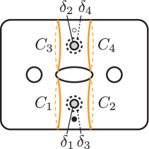
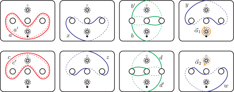
Refer to caption
Figure 12. The curves Ci,δisubscript𝐶𝑖subscript𝛿𝑖C_{i},\delta_{i} on Σ3,24superscriptsubscriptΣ324\Sigma_{3,2}^{4}.
Refer to caption
Figure 13. Vanishing cycles of the genus–333 pencil.

By cyclic permutations, we can rewrite the relations as

t\scaletod9ptt\scaletow9ptt\scaletoa9ptt\scaletoa9ptt\scaletox9ptt\scaletob9pt𝒫α1=t\scaletoδ19ptt\scaletoδ29ptt\scaletoC39ptt\scaletoC49ptt\scaletoC29pt1t\scaletoC19pt1,subscript𝑡\scaletosuperscript𝑑9𝑝𝑡subscript𝑡\scaleto𝑤9𝑝𝑡subscript𝑡\scaleto𝑎9𝑝𝑡subscript𝑡\scaletosuperscript𝑎9𝑝𝑡subscript𝑡\scaleto𝑥9𝑝𝑡subscript𝑡\scaleto𝑏9𝑝𝑡subscript𝒫subscript𝛼1subscript𝑡\scaletosubscript𝛿19𝑝𝑡subscript𝑡\scaletosubscript𝛿29𝑝𝑡subscript𝑡\scaletosubscript𝐶39𝑝𝑡subscript𝑡\scaletosubscript𝐶49𝑝𝑡superscriptsubscript𝑡\scaletosubscript𝐶29𝑝𝑡1superscriptsubscript𝑡\scaletosubscript𝐶19𝑝𝑡1\displaystyle t_{\scaleto{\mathstrut d^{\prime}}{9pt}}t_{\scaleto{\mathstrut w}{9pt}}t_{\scaleto{\mathstrut a}{9pt}}t_{\scaleto{\mathstrut a^{\prime}}{9pt}}t_{\scaleto{\mathstrut x}{9pt}}t_{\scaleto{\mathstrut b}{9pt}}\cdot\mathcal{P}_{\vec{\alpha}_{1}}=t_{\scaleto{\mathstrut\delta_{1}}{9pt}}t_{\scaleto{\mathstrut\delta_{2}}{9pt}}t_{\scaleto{\mathstrut C_{3}}{9pt}}t_{\scaleto{\mathstrut C_{4}}{9pt}}t_{\scaleto{\mathstrut C_{2}}{9pt}}^{-1}t_{\scaleto{\mathstrut C_{1}}{9pt}}^{-1},
t\scaletob9ptt\scaletoy9ptt\scaletoc9ptt\scaletoc9ptt\scaletoz9ptt\scaletod9pt𝒫α2=t\scaletoδ39ptt\scaletoδ49ptt\scaletoC19ptt\scaletoC29ptt\scaletoC49pt1t\scaletoC39pt1.subscript𝑡\scaletosuperscript𝑏9𝑝𝑡subscript𝑡\scaleto𝑦9𝑝𝑡subscript𝑡\scaleto𝑐9𝑝𝑡subscript𝑡\scaletosuperscript𝑐9𝑝𝑡subscript𝑡\scaleto𝑧9𝑝𝑡subscript𝑡\scaleto𝑑9𝑝𝑡subscript𝒫subscript𝛼2subscript𝑡\scaletosubscript𝛿39𝑝𝑡subscript𝑡\scaletosubscript𝛿49𝑝𝑡subscript𝑡\scaletosubscript𝐶19𝑝𝑡subscript𝑡\scaletosubscript𝐶29𝑝𝑡superscriptsubscript𝑡\scaletosubscript𝐶49𝑝𝑡1superscriptsubscript𝑡\scaletosubscript𝐶39𝑝𝑡1\displaystyle t_{\scaleto{\mathstrut b^{\prime}}{9pt}}t_{\scaleto{\mathstrut y}{9pt}}t_{\scaleto{\mathstrut c}{9pt}}t_{\scaleto{\mathstrut c^{\prime}}{9pt}}t_{\scaleto{\mathstrut z}{9pt}}t_{\scaleto{\mathstrut d}{9pt}}\cdot\mathcal{P}_{\vec{\alpha}_{2}}=t_{\scaleto{\mathstrut\delta_{3}}{9pt}}t_{\scaleto{\mathstrut\delta_{4}}{9pt}}t_{\scaleto{\mathstrut C_{1}}{9pt}}t_{\scaleto{\mathstrut C_{2}}{9pt}}t_{\scaleto{\mathstrut C_{4}}{9pt}}^{-1}t_{\scaleto{\mathstrut C_{3}}{9pt}}^{-1}.

Combining them we get

t\scaletod9ptt\scaletow9ptt\scaletoa9ptt\scaletoa9ptt\scaletox9ptt\scaletob9pt𝒫α1t\scaletob9ptt\scaletoy9ptt\scaletoc9ptt\scaletoc9ptt\scaletoz9ptt\scaletod9pt𝒫α2=t\scaletoδ19ptt\scaletoδ29ptt\scaletoδ39ptt\scaletoδ49pt,subscript𝑡\scaletosuperscript𝑑9𝑝𝑡subscript𝑡\scaleto𝑤9𝑝𝑡subscript𝑡\scaleto𝑎9𝑝𝑡subscript𝑡\scaletosuperscript𝑎9𝑝𝑡subscript𝑡\scaleto𝑥9𝑝𝑡subscript𝑡\scaleto𝑏9𝑝𝑡subscript𝒫subscript𝛼1subscript𝑡\scaletosuperscript𝑏9𝑝𝑡subscript𝑡\scaleto𝑦9𝑝𝑡subscript𝑡\scaleto𝑐9𝑝𝑡subscript𝑡\scaletosuperscript𝑐9𝑝𝑡subscript𝑡\scaleto𝑧9𝑝𝑡subscript𝑡\scaleto𝑑9𝑝𝑡subscript𝒫subscript𝛼2subscript𝑡\scaletosubscript𝛿19𝑝𝑡subscript𝑡\scaletosubscript𝛿29𝑝𝑡subscript𝑡\scaletosubscript𝛿39𝑝𝑡subscript𝑡\scaletosubscript𝛿49𝑝𝑡\displaystyle t_{\scaleto{\mathstrut d^{\prime}}{9pt}}t_{\scaleto{\mathstrut w}{9pt}}t_{\scaleto{\mathstrut a}{9pt}}t_{\scaleto{\mathstrut a^{\prime}}{9pt}}t_{\scaleto{\mathstrut x}{9pt}}t_{\scaleto{\mathstrut b}{9pt}}\cdot\mathcal{P}_{\vec{\alpha}_{1}}\cdot t_{\scaleto{\mathstrut b^{\prime}}{9pt}}t_{\scaleto{\mathstrut y}{9pt}}t_{\scaleto{\mathstrut c}{9pt}}t_{\scaleto{\mathstrut c^{\prime}}{9pt}}t_{\scaleto{\mathstrut z}{9pt}}t_{\scaleto{\mathstrut d}{9pt}}\cdot\mathcal{P}_{\vec{\alpha}_{2}}=t_{\scaleto{\mathstrut\delta_{1}}{9pt}}t_{\scaleto{\mathstrut\delta_{2}}{9pt}}t_{\scaleto{\mathstrut\delta_{3}}{9pt}}t_{\scaleto{\mathstrut\delta_{4}}{9pt}},

which, using cyclic permutation and commutativity, can be expressed as

(9) t\scaletoa9ptt\scaletoa9ptt\scaletox9ptt\scaletob9ptt\scaletob9ptt\scaletoy9ptt\scaletoc9ptt\scaletoc9ptt\scaletoz9ptt\scaletod9ptt\scaletod9ptt\scaletow9pt𝒫α1𝒫α2=t\scaletoδ19ptt\scaletoδ29ptt\scaletoδ39ptt\scaletoδ49pt.subscript𝑡\scaleto𝑎9𝑝𝑡subscript𝑡\scaletosuperscript𝑎9𝑝𝑡subscript𝑡\scaleto𝑥9𝑝𝑡subscript𝑡\scaleto𝑏9𝑝𝑡subscript𝑡\scaletosuperscript𝑏9𝑝𝑡subscript𝑡\scaleto𝑦9𝑝𝑡subscript𝑡\scaleto𝑐9𝑝𝑡subscript𝑡\scaletosuperscript𝑐9𝑝𝑡subscript𝑡\scaleto𝑧9𝑝𝑡subscript𝑡\scaleto𝑑9𝑝𝑡subscript𝑡\scaletosuperscript𝑑9𝑝𝑡subscript𝑡\scaleto𝑤9𝑝𝑡subscript𝒫subscript𝛼1subscript𝒫subscript𝛼2subscript𝑡\scaletosubscript𝛿19𝑝𝑡subscript𝑡\scaletosubscript𝛿29𝑝𝑡subscript𝑡\scaletosubscript𝛿39𝑝𝑡subscript𝑡\scaletosubscript𝛿49𝑝𝑡\displaystyle t_{\scaleto{\mathstrut a}{9pt}}t_{\scaleto{\mathstrut a^{\prime}}{9pt}}t_{\scaleto{\mathstrut x}{9pt}}t_{\scaleto{\mathstrut b}{9pt}}t_{\scaleto{\mathstrut b^{\prime}}{9pt}}t_{\scaleto{\mathstrut y}{9pt}}t_{\scaleto{\mathstrut c}{9pt}}t_{\scaleto{\mathstrut c^{\prime}}{9pt}}t_{\scaleto{\mathstrut z}{9pt}}t_{\scaleto{\mathstrut d}{9pt}}t_{\scaleto{\mathstrut d^{\prime}}{9pt}}t_{\scaleto{\mathstrut w}{9pt}}\cdot\mathcal{P}_{\vec{\alpha}_{1}}\mathcal{P}_{\vec{\alpha}_{2}}=t_{\scaleto{\mathstrut\delta_{1}}{9pt}}t_{\scaleto{\mathstrut\delta_{2}}{9pt}}t_{\scaleto{\mathstrut\delta_{3}}{9pt}}t_{\scaleto{\mathstrut\delta_{4}}{9pt}}.

This is a relation in Mod(Σ3,24)ModsuperscriptsubscriptΣ324\operatorname{Mod}(\Sigma_{3,2}^{4}), which, by forgetting the marked points, reduces to the positive factorization of a genus–333 pencil.

In the relation (9), we have the two bounding pairs a,a𝑎superscript𝑎a,a^{\prime} and c,c𝑐superscript𝑐c,c^{\prime}, which are inherited from the genus–222 pencil. There are two more bounding pairs b,b𝑏superscript𝑏b,b^{\prime} and d,d𝑑superscript𝑑d,d^{\prime}; see Figure 13. (The existence of these four bounding pairs is the most essential feature for our constructing of the signature zero Lefschetz fibration in the next subsection.) There is in fact a fifth bounding pair we can get after Hurwitz moves: We can move the factor t\scaletox9ptsubscript𝑡\scaleto𝑥9𝑝𝑡t_{\scaleto{\mathstrut x}{9pt}} over the subword t\scaletob9ptt\scaletob9ptt\scaletoy9ptt\scaletoc9ptt\scaletoc9ptsubscript𝑡\scaleto𝑏9𝑝𝑡subscript𝑡\scaletosuperscript𝑏9𝑝𝑡subscript𝑡\scaleto𝑦9𝑝𝑡subscript𝑡\scaleto𝑐9𝑝𝑡subscript𝑡\scaletosuperscript𝑐9𝑝𝑡t_{\scaleto{\mathstrut b}{9pt}}t_{\scaleto{\mathstrut b^{\prime}}{9pt}}t_{\scaleto{\mathstrut y}{9pt}}t_{\scaleto{\mathstrut c}{9pt}}t_{\scaleto{\mathstrut c^{\prime}}{9pt}} (i.e. we conjugate this subword with t\scaletox9ptsubscript𝑡\scaleto𝑥9𝑝𝑡t_{\scaleto{\mathstrut x}{9pt}}) to get the subword t\scaletox9ptt\scaletoz9ptsubscript𝑡\scaleto𝑥9𝑝𝑡subscript𝑡\scaleto𝑧9𝑝𝑡t_{\scaleto{\mathstrut x}{9pt}}t_{\scaleto{\mathstrut z}{9pt}} in the monodromy, where the pair x,z𝑥𝑧x,z too splits the surface into two genus–111 subsurfaces. (Note that the pair y,w𝑦𝑤y,w is yet another bounding pair, but this property is destroyed when we bring t\scaletox9ptsubscript𝑡\scaleto𝑥9𝑝𝑡t_{\scaleto{\mathstrut x}{9pt}} and t\scaletoz9ptsubscript𝑡\scaleto𝑧9𝑝𝑡t_{\scaleto{\mathstrut z}{9pt}} together above.)

The total space Y𝑌Y of our genus–333 pencil has signature zero since the relation (9) is the combination of two copies of the relation (7) with signature zero. The Euler characteristic is easily calculated as e(Y)=44g+lb=443+124=0e𝑌44𝑔𝑙𝑏4431240{\text{e}}(Y)=4-4g+l-b=4-4\cdot 3+12-4=0 (where g𝑔g is the fiber genus, l𝑙l is the number of Lefschetz critical points and b𝑏b is the number of base points).

To pin down the topology of Y𝑌Y we will calculate its first homology. Let us use the symplectic basis {α1,β1,α2,β2,α3,β3}subscript𝛼1subscript𝛽1subscript𝛼2subscript𝛽2subscript𝛼3subscript𝛽3\{\alpha_{1},\beta_{1},\alpha_{2},\beta_{2},\alpha_{3},\beta_{3}\} for H1(Σ4;)subscript𝐻1subscriptΣ4H_{1}(\Sigma_{4};\mathbb{Z}) as in Figure 14.

Refer to caption
Figure 14. The basis for H1(Σ4;)subscript𝐻1subscriptΣ4H_{1}(\Sigma_{4};\mathbb{Z}).

The homology classes of the vanishing cycles in this basis are: a=a=c=c=α1+α3𝑎superscript𝑎𝑐superscript𝑐subscript𝛼1subscript𝛼3a=a^{\prime}=c=c^{\prime}=\alpha_{1}+\alpha_{3},  x=z=α1+α3β1+β2β3𝑥𝑧subscript𝛼1subscript𝛼3subscript𝛽1subscript𝛽2subscript𝛽3x=z=\alpha_{1}+\alpha_{3}-\beta_{1}+\beta_{2}-\beta_{3},  b=b=d=d=β1β2+β3𝑏superscript𝑏𝑑superscript𝑑subscript𝛽1subscript𝛽2subscript𝛽3b=b^{\prime}=d=d^{\prime}=\beta_{1}-\beta_{2}+\beta_{3}  and y=w=α1+α3+β1β2+β3𝑦𝑤subscript𝛼1subscript𝛼3subscript𝛽1subscript𝛽2subscript𝛽3y=w=\alpha_{1}+\alpha_{3}+\beta_{1}-\beta_{2}+\beta_{3}. In turn, the relations in H1(Y;)subscript𝐻1𝑌H_{1}(Y;\mathbb{Z}) we obtain by setting the vanishing cycles equal to zero are: α3=α1subscript𝛼3subscript𝛼1\alpha_{3}=-\alpha_{1}  and β3=β1+β2subscript𝛽3subscript𝛽1subscript𝛽2\beta_{3}=-\beta_{1}+\beta_{2}. Therefore H1(Y;)subscript𝐻1𝑌H_{1}(Y;\mathbb{Z}) is freely generated by α1,β1,α2,β2subscript𝛼1subscript𝛽1subscript𝛼2subscript𝛽2\alpha_{1},\beta_{1},\alpha_{2},\beta_{2}, and H1(Y;)=4subscript𝐻1𝑌superscript4H_{1}(Y;\mathbb{Z})=\mathbb{Z}^{4}.

Since σ(Y)=e(Y)𝜎𝑌e𝑌\sigma(Y)={\text{e}}(Y) and b1(Y)=4subscript𝑏1𝑌4b_{1}(Y)=4, Y𝑌Y cannot be a rational or ruled surface. Since this genus–333 pencil has 444 base points, by [13, Theorem 1.2], Y𝑌Y is a symplectic Calabi-Yau 444–manifold, rational homology equivalent to T4superscript𝑇4T^{4}. (In fact one can show that π1(Y)4subscript𝜋1𝑌superscript4\pi_{1}(Y)\cong\mathbb{Z}^{4} and thus Y𝑌Y is homeomorphic to T4superscript𝑇4T^{4}.) In particular we see that Y𝑌Y is spin. Alternatively, one can directly construct a quadratic form on Σ34superscriptsubscriptΣ34\Sigma_{3}^{4} that satisfies the conditions in Theorem 1 to show Y𝑌Y is spin.

Remark 13.

There are other explicit monodromy factorizations for genus–333 pencils with four base points on symplectic Calabi-Yau 444–manifolds homeomorphic to T4superscript𝑇4T^{4}, obtained by the first author in [12] and the second author and Hayano in [33]. It is once again natural to ask whether the one we discovered here is Hurwitz equivalent to any of those, and we will also confirm that this is the case in Appendix A, which in particular will imply that this 444–manifold Y𝑌Y is diffeomorphic to the standard T4superscript𝑇4T^{4}.

3.3. A signature zero genus–999 Lefschetz fibration over the 222–sphere

We will now describe our genus–999 fibration (X,f)𝑋𝑓(X,f), the total space of which has signature zero. Further properties of X𝑋X, such as it being spin, will be explored in Section 4.1. Expectedly, its monodromy factorization will not contain any Dehn twists along separating curves (which would destroy the spin property), but it contains Dehn twists along a quadruple of bounding curves which split the Σ9subscriptΣ9\Sigma_{9} into two copies of Σ34superscriptsubscriptΣ34\Sigma_{3}^{4}. This extra property will be essential for our arguments in Section 5.

We will first explain how we obtain our signature zero Lefschetz fibration, without specifying all the embeddings involved in this construction, and thus without an explicit description of all the curves in the final monodromy factorization. We will also omit the marked point in this exposition. This first round of information suffices to justify the existence of a signature zero genus–999 Lefschetz fibration. Afterwards, we will describe the embeddings explicitly, and also include the marked point for the pseudosection calculation. The latter will take the chunk of this subsection.

Schematic construction: For simplicity, we omit all the marked points in any of the figures we will refer to here. We will breed six copies of our genus–333 pencil with monodromy factorization (9). As seen on the right side of Figure 16, the curves Δ1,Δ2,Δ3,Δ4subscriptΔ1subscriptΔ2subscriptΔ3subscriptΔ4\Delta_{1},\Delta_{2},\Delta_{3},\Delta_{4} on Σ9subscriptΣ9\Sigma_{9} bound two copies of Σ34superscriptsubscriptΣ34\Sigma_{3}^{4}, which constitute the top and the bottom halves of Σ9subscriptΣ9\Sigma_{9}. We embed two copies of the relation (9) in Mod(Σ34)ModsuperscriptsubscriptΣ34\operatorname{Mod}(\Sigma_{3}^{4}) into Mod(Σ9)ModsubscriptΣ9\operatorname{Mod}(\Sigma_{9}) via the embeddings Φ1subscriptΦ1\Phi_{1} and Φ2subscriptΦ2\Phi_{2} as explained in Figure 16 (and its caption), such that the first one is supported on the top and the second one on the bottom half:

t\scaletoa19ptt\scaletoa19ptt\scaletox19ptt\scaletob19ptt\scaletob19ptt\scaletoy19ptt\scaletoc19ptt\scaletoc19ptt\scaletoz19ptt\scaletod19ptt\scaletod19ptt\scaletow19pt=t\scaletoΔ19ptt\scaletoΔ29ptt\scaletoΔ39ptt\scaletoΔ49pt,subscript𝑡\scaletosubscript𝑎19𝑝𝑡subscript𝑡\scaletosuperscriptsubscript𝑎19𝑝𝑡subscript𝑡\scaletosubscript𝑥19𝑝𝑡subscript𝑡\scaletosubscript𝑏19𝑝𝑡subscript𝑡\scaletosuperscriptsubscript𝑏19𝑝𝑡subscript𝑡\scaletosubscript𝑦19𝑝𝑡subscript𝑡\scaletosubscript𝑐19𝑝𝑡subscript𝑡\scaletosuperscriptsubscript𝑐19𝑝𝑡subscript𝑡\scaletosubscript𝑧19𝑝𝑡subscript𝑡\scaletosubscript𝑑19𝑝𝑡subscript𝑡\scaletosuperscriptsubscript𝑑19𝑝𝑡subscript𝑡\scaletosubscript𝑤19𝑝𝑡subscript𝑡\scaletosubscriptΔ19𝑝𝑡subscript𝑡\scaletosubscriptΔ29𝑝𝑡subscript𝑡\scaletosubscriptΔ39𝑝𝑡subscript𝑡\scaletosubscriptΔ49𝑝𝑡\displaystyle t_{\scaleto{\mathstrut a_{1}}{9pt}}t_{\scaleto{\mathstrut a_{1}^{\prime}}{9pt}}t_{\scaleto{\mathstrut x_{1}}{9pt}}t_{\scaleto{\mathstrut b_{1}}{9pt}}t_{\scaleto{\mathstrut b_{1}^{\prime}}{9pt}}t_{\scaleto{\mathstrut y_{1}}{9pt}}t_{\scaleto{\mathstrut c_{1}}{9pt}}t_{\scaleto{\mathstrut c_{1}^{\prime}}{9pt}}t_{\scaleto{\mathstrut z_{1}}{9pt}}t_{\scaleto{\mathstrut d_{1}}{9pt}}t_{\scaleto{\mathstrut d_{1}^{\prime}}{9pt}}t_{\scaleto{\mathstrut w_{1}}{9pt}}=t_{\scaleto{\mathstrut\Delta_{1}}{9pt}}t_{\scaleto{\mathstrut\Delta_{2}}{9pt}}t_{\scaleto{\mathstrut\Delta_{3}}{9pt}}t_{\scaleto{\mathstrut\Delta_{4}}{9pt}},
t\scaletoa29ptt\scaletoa29ptt\scaletox29ptt\scaletob29ptt\scaletob29ptt\scaletoy29ptt\scaletoc29ptt\scaletoc29ptt\scaletoz29ptt\scaletod29ptt\scaletod29ptt\scaletow29pt=t\scaletoΔ19ptt\scaletoΔ29ptt\scaletoΔ39ptt\scaletoΔ49pt.subscript𝑡\scaletosubscript𝑎29𝑝𝑡subscript𝑡\scaletosuperscriptsubscript𝑎29𝑝𝑡subscript𝑡\scaletosubscript𝑥29𝑝𝑡subscript𝑡\scaletosubscript𝑏29𝑝𝑡subscript𝑡\scaletosuperscriptsubscript𝑏29𝑝𝑡subscript𝑡\scaletosubscript𝑦29𝑝𝑡subscript𝑡\scaletosubscript𝑐29𝑝𝑡subscript𝑡\scaletosuperscriptsubscript𝑐29𝑝𝑡subscript𝑡\scaletosubscript𝑧29𝑝𝑡subscript𝑡\scaletosubscript𝑑29𝑝𝑡subscript𝑡\scaletosuperscriptsubscript𝑑29𝑝𝑡subscript𝑡\scaletosubscript𝑤29𝑝𝑡subscript𝑡\scaletosubscriptΔ19𝑝𝑡subscript𝑡\scaletosubscriptΔ29𝑝𝑡subscript𝑡\scaletosubscriptΔ39𝑝𝑡subscript𝑡\scaletosubscriptΔ49𝑝𝑡\displaystyle t_{\scaleto{\mathstrut a_{2}}{9pt}}t_{\scaleto{\mathstrut a_{2}^{\prime}}{9pt}}t_{\scaleto{\mathstrut x_{2}}{9pt}}t_{\scaleto{\mathstrut b_{2}}{9pt}}t_{\scaleto{\mathstrut b_{2}^{\prime}}{9pt}}t_{\scaleto{\mathstrut y_{2}}{9pt}}t_{\scaleto{\mathstrut c_{2}}{9pt}}t_{\scaleto{\mathstrut c_{2}^{\prime}}{9pt}}t_{\scaleto{\mathstrut z_{2}}{9pt}}t_{\scaleto{\mathstrut d_{2}}{9pt}}t_{\scaleto{\mathstrut d_{2}^{\prime}}{9pt}}t_{\scaleto{\mathstrut w_{2}}{9pt}}=t_{\scaleto{\mathstrut\Delta_{1}}{9pt}}t_{\scaleto{\mathstrut\Delta_{2}}{9pt}}t_{\scaleto{\mathstrut\Delta_{3}}{9pt}}t_{\scaleto{\mathstrut\Delta_{4}}{9pt}}.

These curves are explicitly given in Figures 16 and 23. As usual, the Dehn twist curves in the two relations above are the images, under the respective embeddings Φ1subscriptΦ1\Phi_{1} and Φ2subscriptΦ2\Phi_{2}, of the curves of the relation (9) in the same order – and the same goes for our four other embeddings to follow.

[Uncaptioned image]
Figure 15. The embedding Φ1subscriptΦ1\Phi_{1} of Σ34superscriptsubscriptΣ34\Sigma_{3}^{4} into Σ9subscriptΣ9\Sigma_{9}. First, we slide the four boundary components as indicated by the blue arrows. Then embed the surface into the top half of Σ9subscriptΣ9\Sigma_{9}. The labels 1,2,3,412341,2,3,4 indicate how the boundary components are matched with the quadruple Δ1,Δ2,Δ3,Δ4subscriptΔ1subscriptΔ2subscriptΔ3subscriptΔ4\Delta_{1},\Delta_{2},\Delta_{3},\Delta_{4}. Also, the gray curves, which fill Σ34superscriptsubscriptΣ34\Sigma_{3}^{4}, and their embedded images are drawn so that the embedding Φ1subscriptΦ1\Phi_{1} is uniquely defined. The second embedding Φ2subscriptΦ2\Phi_{2} is given by Φ1subscriptΦ1\Phi_{1} followed by the π𝜋\pi–rotation r𝑟r, that is Φ2:=rΦ1assignsubscriptΦ2𝑟subscriptΦ1\Phi_{2}:=r\circ\Phi_{1}.
[Uncaptioned image]
Figure 16. The four bounding quadruples.

Since these two relations have disjoint supports, we can combine them to get

t\scaletoa19ptt\scaletoa19ptt\scaletoa29ptt\scaletoa29ptt\scaletox19ptt\scaletox29ptt\scaletob19ptt\scaletob19ptt\scaletob29ptt\scaletob29ptt\scaletoy19ptt\scaletoy29ptt\scaletoc19ptt\scaletoc19ptt\scaletoc29ptt\scaletoc29ptt\scaletoz19ptt\scaletoz29ptt\scaletod19ptt\scaletod19ptt\scaletod29ptt\scaletod29ptt\scaletow19ptt\scaletow29pt=t\scaletoΔ19pt2t\scaletoΔ29pt2t\scaletoΔ39pt2t\scaletoΔ49pt2,subscript𝑡\scaletosubscript𝑎19𝑝𝑡subscript𝑡\scaletosuperscriptsubscript𝑎19𝑝𝑡subscript𝑡\scaletosubscript𝑎29𝑝𝑡subscript𝑡\scaletosuperscriptsubscript𝑎29𝑝𝑡subscript𝑡\scaletosubscript𝑥19𝑝𝑡subscript𝑡\scaletosubscript𝑥29𝑝𝑡subscript𝑡\scaletosubscript𝑏19𝑝𝑡subscript𝑡\scaletosuperscriptsubscript𝑏19𝑝𝑡subscript𝑡\scaletosubscript𝑏29𝑝𝑡subscript𝑡\scaletosuperscriptsubscript𝑏29𝑝𝑡subscript𝑡\scaletosubscript𝑦19𝑝𝑡subscript𝑡\scaletosubscript𝑦29𝑝𝑡subscript𝑡\scaletosubscript𝑐19𝑝𝑡subscript𝑡\scaletosuperscriptsubscript𝑐19𝑝𝑡subscript𝑡\scaletosubscript𝑐29𝑝𝑡subscript𝑡\scaletosuperscriptsubscript𝑐29𝑝𝑡subscript𝑡\scaletosubscript𝑧19𝑝𝑡subscript𝑡\scaletosubscript𝑧29𝑝𝑡subscript𝑡\scaletosubscript𝑑19𝑝𝑡subscript𝑡\scaletosuperscriptsubscript𝑑19𝑝𝑡subscript𝑡\scaletosubscript𝑑29𝑝𝑡subscript𝑡\scaletosuperscriptsubscript𝑑29𝑝𝑡subscript𝑡\scaletosubscript𝑤19𝑝𝑡subscript𝑡\scaletosubscript𝑤29𝑝𝑡superscriptsubscript𝑡\scaletosubscriptΔ19𝑝𝑡2superscriptsubscript𝑡\scaletosubscriptΔ29𝑝𝑡2superscriptsubscript𝑡\scaletosubscriptΔ39𝑝𝑡2superscriptsubscript𝑡\scaletosubscriptΔ49𝑝𝑡2\displaystyle t_{\scaleto{\mathstrut a_{1}}{9pt}}t_{\scaleto{\mathstrut a_{1}^{\prime}}{9pt}}t_{\scaleto{\mathstrut a_{2}}{9pt}}t_{\scaleto{\mathstrut a_{2}^{\prime}}{9pt}}t_{\scaleto{\mathstrut x_{1}}{9pt}}t_{\scaleto{\mathstrut x_{2}}{9pt}}t_{\scaleto{\mathstrut b_{1}}{9pt}}t_{\scaleto{\mathstrut b_{1}^{\prime}}{9pt}}t_{\scaleto{\mathstrut b_{2}}{9pt}}t_{\scaleto{\mathstrut b_{2}^{\prime}}{9pt}}t_{\scaleto{\mathstrut y_{1}}{9pt}}t_{\scaleto{\mathstrut y_{2}}{9pt}}t_{\scaleto{\mathstrut c_{1}}{9pt}}t_{\scaleto{\mathstrut c_{1}^{\prime}}{9pt}}t_{\scaleto{\mathstrut c_{2}}{9pt}}t_{\scaleto{\mathstrut c_{2}^{\prime}}{9pt}}t_{\scaleto{\mathstrut z_{1}}{9pt}}t_{\scaleto{\mathstrut z_{2}}{9pt}}t_{\scaleto{\mathstrut d_{1}}{9pt}}t_{\scaleto{\mathstrut d_{1}^{\prime}}{9pt}}t_{\scaleto{\mathstrut d_{2}}{9pt}}t_{\scaleto{\mathstrut d_{2}^{\prime}}{9pt}}t_{\scaleto{\mathstrut w_{1}}{9pt}}t_{\scaleto{\mathstrut w_{2}}{9pt}}=t_{\scaleto{\mathstrut\Delta_{1}}{9pt}}^{2}t_{\scaleto{\mathstrut\Delta_{2}}{9pt}}^{2}t_{\scaleto{\mathstrut\Delta_{3}}{9pt}}^{2}t_{\scaleto{\mathstrut\Delta_{4}}{9pt}}^{2},

in Mod(Σ9)ModsubscriptΣ9\operatorname{Mod}(\Sigma_{9}), which we can rewrite as

(10) t\scaletoa19ptt\scaletoa19ptt\scaletoa29ptt\scaletoa29ptt\scaletoΔ19pt1t\scaletoΔ49pt1¯t\scaletox19ptt\scaletox29ptt\scaletob19ptt\scaletob19ptt\scaletob29ptt\scaletob29ptt\scaletoΔ39pt1t\scaletoΔ49pt1¯t\scaletoy19ptt\scaletoy29pt¯subscript𝑡\scaletosubscript𝑎19𝑝𝑡subscript𝑡\scaletosuperscriptsubscript𝑎19𝑝𝑡subscript𝑡\scaletosubscript𝑎29𝑝𝑡subscript𝑡\scaletosuperscriptsubscript𝑎29𝑝𝑡superscriptsubscript𝑡\scaletosubscriptΔ19𝑝𝑡1superscriptsubscript𝑡\scaletosubscriptΔ49𝑝𝑡1subscript𝑡\scaletosubscript𝑥19𝑝𝑡subscript𝑡\scaletosubscript𝑥29𝑝𝑡¯subscript𝑡\scaletosubscript𝑏19𝑝𝑡subscript𝑡\scaletosuperscriptsubscript𝑏19𝑝𝑡subscript𝑡\scaletosubscript𝑏29𝑝𝑡subscript𝑡\scaletosuperscriptsubscript𝑏29𝑝𝑡superscriptsubscript𝑡\scaletosubscriptΔ39𝑝𝑡1superscriptsubscript𝑡\scaletosubscriptΔ49𝑝𝑡1subscript𝑡\scaletosubscript𝑦19𝑝𝑡subscript𝑡\scaletosubscript𝑦29𝑝𝑡\displaystyle\underline{t_{\scaleto{\mathstrut a_{1}}{9pt}}t_{\scaleto{\mathstrut a_{1}^{\prime}}{9pt}}t_{\scaleto{\mathstrut a_{2}}{9pt}}t_{\scaleto{\mathstrut a_{2}^{\prime}}{9pt}}t_{\scaleto{\mathstrut\Delta_{1}}{9pt}}^{-1}t_{\scaleto{\mathstrut\Delta_{4}}{9pt}}^{-1}}\cdot t_{\scaleto{\mathstrut x_{1}}{9pt}}t_{\scaleto{\mathstrut x_{2}}{9pt}}\cdot\underline{t_{\scaleto{\mathstrut b_{1}}{9pt}}t_{\scaleto{\mathstrut b_{1}^{\prime}}{9pt}}t_{\scaleto{\mathstrut b_{2}}{9pt}}t_{\scaleto{\mathstrut b_{2}^{\prime}}{9pt}}t_{\scaleto{\mathstrut\Delta_{3}}{9pt}}^{-1}t_{\scaleto{\mathstrut\Delta_{4}}{9pt}}^{-1}}\cdot t_{\scaleto{\mathstrut y_{1}}{9pt}}t_{\scaleto{\mathstrut y_{2}}{9pt}}
t\scaletoc19ptt\scaletoc19ptt\scaletoc29ptt\scaletoc29ptt\scaletoΔ29pt1t\scaletoΔ39pt1¯t\scaletoz19ptt\scaletoz29ptt\scaletod19ptt\scaletod19ptt\scaletod29ptt\scaletod29ptt\scaletoΔ19pt1t\scaletoΔ29pt1¯t\scaletow19ptt\scaletow29pt=1.\displaystyle\cdot\underline{t_{\scaleto{\mathstrut c_{1}}{9pt}}t_{\scaleto{\mathstrut c_{1}^{\prime}}{9pt}}t_{\scaleto{\mathstrut c_{2}}{9pt}}t_{\scaleto{\mathstrut c_{2}^{\prime}}{9pt}}t_{\scaleto{\mathstrut\Delta_{2}}{9pt}}^{-1}t_{\scaleto{\mathstrut\Delta_{3}}{9pt}}^{-1}}\cdot t_{\scaleto{\mathstrut z_{1}}{9pt}}t_{\scaleto{\mathstrut z_{2}}{9pt}}\cdot\underline{t_{\scaleto{\mathstrut d_{1}}{9pt}}t_{\scaleto{\mathstrut d_{1}^{\prime}}{9pt}}t_{\scaleto{\mathstrut d_{2}}{9pt}}t_{\scaleto{\mathstrut d_{2}^{\prime}}{9pt}}t_{\scaleto{\mathstrut\Delta_{1}}{9pt}}^{-1}t_{\scaleto{\mathstrut\Delta_{2}}{9pt}}^{-1}}\cdot t_{\scaleto{\mathstrut w_{1}}{9pt}}t_{\scaleto{\mathstrut w_{2}}{9pt}}=1.

The most essential feature of this relation is that it contains Dehn twists along four bounding quadruples, as singled out in Figure 16, such that the subsurfaces they cobound are diffeomorphic to Σ34superscriptsubscriptΣ34\Sigma_{3}^{4} with pairs of ΔisubscriptΔ𝑖\Delta_{i} as genus–111 bounding pairs in each Σ34superscriptsubscriptΣ34\Sigma_{3}^{4}.

Now, let us examine the configuration of the curves a1,a1,a2,a2,Δ1,Δ4subscript𝑎1superscriptsubscript𝑎1subscript𝑎2superscriptsubscript𝑎2subscriptΔ1subscriptΔ4a_{1},a_{1}^{\prime},a_{2},a_{2}^{\prime},\Delta_{1},\Delta_{4}. Let S3subscript𝑆3S_{3} be the subsurface bounded by the quadruple a1,a1,a2,a2subscript𝑎1superscriptsubscript𝑎1subscript𝑎2superscriptsubscript𝑎2a_{1},a_{1}^{\prime},a_{2},a_{2}^{\prime} that contains Δ1subscriptΔ1\Delta_{1} and Δ4subscriptΔ4\Delta_{4}. Then it is easy to observe that S3subscript𝑆3S_{3} is diffeomorphic to Σ34superscriptsubscriptΣ34\Sigma_{3}^{4} and the pair Δ1,Δ4subscriptΔ1subscriptΔ4\Delta_{1},\Delta_{4} splits S3subscript𝑆3S_{3} into two genus–111 subsurfaces with the boundary components a1,a1,Δ1,Δ4subscript𝑎1superscriptsubscript𝑎1subscriptΔ1subscriptΔ4a_{1},a_{1}^{\prime},\Delta_{1},\Delta_{4} and a2,a2,Δ1,Δ4subscript𝑎2superscriptsubscript𝑎2subscriptΔ1subscriptΔ4a_{2},a_{2}^{\prime},\Delta_{1},\Delta_{4}, respectively. Turning to Figure 13 we note that the pair d,d𝑑superscript𝑑d,d^{\prime} also splits Σ34superscriptsubscriptΣ34\Sigma_{3}^{4} into two genus–111 subsurfaces with the boundary components δ1,δ2,d,dsubscript𝛿1subscript𝛿2𝑑superscript𝑑\delta_{1},\delta_{2},d,d^{\prime} and δ3,δ4,d,dsubscript𝛿3subscript𝛿4𝑑superscript𝑑\delta_{3},\delta_{4},d,d^{\prime}, respectively. This means that the tuple of curves (a1,a1,a2,a2,Δ1,Δ4(a_{1},a_{1}^{\prime},a_{2},a_{2}^{\prime},\Delta_{1},\Delta_{4}) in S3subscript𝑆3S_{3} is topologically equivalent to (δ1,δ2,δ3,δ4,d,d)subscript𝛿1subscript𝛿2subscript𝛿3subscript𝛿4𝑑superscript𝑑(\delta_{1},\delta_{2},\delta_{3},\delta_{4},d,d^{\prime}) in Σ34superscriptsubscriptΣ34\Sigma_{3}^{4}. Therefore there exists an embedding Φ3subscriptΦ3\Phi_{3} of Σ34superscriptsubscriptΣ34\Sigma_{3}^{4} into Σ9subscriptΣ9\Sigma_{9} such that

  • Φ3subscriptΦ3\Phi_{3} maps (δ1,δ2,δ3,δ4,d,d)subscript𝛿1subscript𝛿2subscript𝛿3subscript𝛿4𝑑superscript𝑑(\delta_{1},\delta_{2},\delta_{3},\delta_{4},d,d^{\prime}) to (a1,a1,a2,a2,Δ1,Δ4)subscript𝑎1superscriptsubscript𝑎1subscript𝑎2superscriptsubscript𝑎2subscriptΔ1subscriptΔ4(a_{1},a_{1}^{\prime},a_{2},a_{2}^{\prime},\Delta_{1},\Delta_{4}).

Identical arguments guarantee that there exist embeddings Φ4,Φ5,Φ6subscriptΦ4subscriptΦ5subscriptΦ6\Phi_{4},\Phi_{5},\Phi_{6} of Σ34superscriptsubscriptΣ34\Sigma_{3}^{4} into Σ9subscriptΣ9\Sigma_{9} such that

  • Φ4subscriptΦ4\Phi_{4} maps (δ1,δ2,δ3,δ4,d,d)subscript𝛿1subscript𝛿2subscript𝛿3subscript𝛿4𝑑superscript𝑑(\delta_{1},\delta_{2},\delta_{3},\delta_{4},d,d^{\prime}) to (b1,b1,b2,b2,Δ3,Δ4)subscript𝑏1superscriptsubscript𝑏1subscript𝑏2superscriptsubscript𝑏2subscriptΔ3subscriptΔ4(b_{1},b_{1}^{\prime},b_{2},b_{2}^{\prime},\Delta_{3},\Delta_{4}),

  • Φ5subscriptΦ5\Phi_{5} maps (δ1,δ2,δ3,δ4,d,d)subscript𝛿1subscript𝛿2subscript𝛿3subscript𝛿4𝑑superscript𝑑(\delta_{1},\delta_{2},\delta_{3},\delta_{4},d,d^{\prime}) to (c1,c1,c2,c2,Δ2,Δ3)subscript𝑐1superscriptsubscript𝑐1subscript𝑐2superscriptsubscript𝑐2subscriptΔ2subscriptΔ3(c_{1},c_{1}^{\prime},c_{2},c_{2}^{\prime},\Delta_{2},\Delta_{3}),

  • Φ6subscriptΦ6\Phi_{6} maps (δ1,δ2,δ3,δ4,d,d)subscript𝛿1subscript𝛿2subscript𝛿3subscript𝛿4𝑑superscript𝑑(\delta_{1},\delta_{2},\delta_{3},\delta_{4},d,d^{\prime}) to (d1,d1,d2,d2,Δ1,Δ2)subscript𝑑1superscriptsubscript𝑑1subscript𝑑2superscriptsubscript𝑑2subscriptΔ1subscriptΔ2(d_{1},d_{1}^{\prime},d_{2},d_{2}^{\prime},\Delta_{1},\Delta_{2}).

Now the genus–333 relation (9) (without marked points) can be rearranged as

t\scaletow9ptt\scaletoa9ptt\scaletoa9ptt\scaletox9ptt\scaletob9ptt\scaletob9ptt\scaletoy9ptt\scaletoc9ptt\scaletoc9ptt\scaletoz9pt=t\scaletoδ19ptt\scaletoδ29ptt\scaletoδ39ptt\scaletoδ49ptt\scaletod9pt1t\scaletod9pt1.subscript𝑡\scaleto𝑤9𝑝𝑡subscript𝑡\scaleto𝑎9𝑝𝑡subscript𝑡\scaletosuperscript𝑎9𝑝𝑡subscript𝑡\scaleto𝑥9𝑝𝑡subscript𝑡\scaleto𝑏9𝑝𝑡subscript𝑡\scaletosuperscript𝑏9𝑝𝑡subscript𝑡\scaleto𝑦9𝑝𝑡subscript𝑡\scaleto𝑐9𝑝𝑡subscript𝑡\scaletosuperscript𝑐9𝑝𝑡subscript𝑡\scaleto𝑧9𝑝𝑡subscript𝑡\scaletosubscript𝛿19𝑝𝑡subscript𝑡\scaletosubscript𝛿29𝑝𝑡subscript𝑡\scaletosubscript𝛿39𝑝𝑡subscript𝑡\scaletosubscript𝛿49𝑝𝑡superscriptsubscript𝑡\scaleto𝑑9𝑝𝑡1superscriptsubscript𝑡\scaletosuperscript𝑑9𝑝𝑡1\displaystyle t_{\scaleto{\mathstrut w}{9pt}}t_{\scaleto{\mathstrut a}{9pt}}t_{\scaleto{\mathstrut a^{\prime}}{9pt}}t_{\scaleto{\mathstrut x}{9pt}}t_{\scaleto{\mathstrut b}{9pt}}t_{\scaleto{\mathstrut b^{\prime}}{9pt}}t_{\scaleto{\mathstrut y}{9pt}}t_{\scaleto{\mathstrut c}{9pt}}t_{\scaleto{\mathstrut c^{\prime}}{9pt}}t_{\scaleto{\mathstrut z}{9pt}}=t_{\scaleto{\mathstrut\delta_{1}}{9pt}}t_{\scaleto{\mathstrut\delta_{2}}{9pt}}t_{\scaleto{\mathstrut\delta_{3}}{9pt}}t_{\scaleto{\mathstrut\delta_{4}}{9pt}}t_{\scaleto{\mathstrut d}{9pt}}^{-1}t_{\scaleto{\mathstrut d^{\prime}}{9pt}}^{-1}.

So if we set ai:=Φi(a),ai:=Φi(a),xi:=Φi(x)formulae-sequenceassignsubscript𝑎𝑖subscriptΦ𝑖𝑎formulae-sequenceassignsuperscriptsubscript𝑎𝑖subscriptΦ𝑖superscript𝑎assignsubscript𝑥𝑖subscriptΦ𝑖𝑥a_{i}:=\Phi_{i}(a),a_{i}^{\prime}:=\Phi_{i}(a^{\prime}),x_{i}:=\Phi_{i}(x), and so on, then copies of this relation are embedded into Γ9subscriptΓ9\Gamma_{9} as

t\scaletow39ptt\scaletoa39ptt\scaletoa39ptt\scaletox39ptt\scaletob39ptt\scaletob39ptt\scaletoy39ptt\scaletoc39ptt\scaletoc39ptt\scaletoz39pt=t\scaletoa19ptt\scaletoa19ptt\scaletoa29ptt\scaletoa29ptt\scaletoΔ19pt1t\scaletoΔ49pt1,subscript𝑡\scaletosubscript𝑤39𝑝𝑡subscript𝑡\scaletosubscript𝑎39𝑝𝑡subscript𝑡\scaletosuperscriptsubscript𝑎39𝑝𝑡subscript𝑡\scaletosubscript𝑥39𝑝𝑡subscript𝑡\scaletosubscript𝑏39𝑝𝑡subscript𝑡\scaletosuperscriptsubscript𝑏39𝑝𝑡subscript𝑡\scaletosubscript𝑦39𝑝𝑡subscript𝑡\scaletosubscript𝑐39𝑝𝑡subscript𝑡\scaletosuperscriptsubscript𝑐39𝑝𝑡subscript𝑡\scaletosubscript𝑧39𝑝𝑡subscript𝑡\scaletosubscript𝑎19𝑝𝑡subscript𝑡\scaletosuperscriptsubscript𝑎19𝑝𝑡subscript𝑡\scaletosubscript𝑎29𝑝𝑡subscript𝑡\scaletosuperscriptsubscript𝑎29𝑝𝑡superscriptsubscript𝑡\scaletosubscriptΔ19𝑝𝑡1superscriptsubscript𝑡\scaletosubscriptΔ49𝑝𝑡1\displaystyle t_{\scaleto{\mathstrut w_{3}}{9pt}}t_{\scaleto{\mathstrut a_{3}}{9pt}}t_{\scaleto{\mathstrut a_{3}^{\prime}}{9pt}}t_{\scaleto{\mathstrut x_{3}}{9pt}}t_{\scaleto{\mathstrut b_{3}}{9pt}}t_{\scaleto{\mathstrut b_{3}^{\prime}}{9pt}}t_{\scaleto{\mathstrut y_{3}}{9pt}}t_{\scaleto{\mathstrut c_{3}}{9pt}}t_{\scaleto{\mathstrut c_{3}^{\prime}}{9pt}}t_{\scaleto{\mathstrut z_{3}}{9pt}}=t_{\scaleto{\mathstrut a_{1}}{9pt}}t_{\scaleto{\mathstrut a_{1}^{\prime}}{9pt}}t_{\scaleto{\mathstrut a_{2}}{9pt}}t_{\scaleto{\mathstrut a_{2}^{\prime}}{9pt}}t_{\scaleto{\mathstrut\Delta_{1}}{9pt}}^{-1}t_{\scaleto{\mathstrut\Delta_{4}}{9pt}}^{-1},
t\scaletow49ptt\scaletoa49ptt\scaletoa49ptt\scaletox49ptt\scaletob49ptt\scaletob49ptt\scaletoy49ptt\scaletoc49ptt\scaletoc49ptt\scaletoz49pt=t\scaletob19ptt\scaletob19ptt\scaletob29ptt\scaletob29ptt\scaletoΔ39pt1t\scaletoΔ49pt1,subscript𝑡\scaletosubscript𝑤49𝑝𝑡subscript𝑡\scaletosubscript𝑎49𝑝𝑡subscript𝑡\scaletosuperscriptsubscript𝑎49𝑝𝑡subscript𝑡\scaletosubscript𝑥49𝑝𝑡subscript𝑡\scaletosubscript𝑏49𝑝𝑡subscript𝑡\scaletosuperscriptsubscript𝑏49𝑝𝑡subscript𝑡\scaletosubscript𝑦49𝑝𝑡subscript𝑡\scaletosubscript𝑐49𝑝𝑡subscript𝑡\scaletosuperscriptsubscript𝑐49𝑝𝑡subscript𝑡\scaletosubscript𝑧49𝑝𝑡subscript𝑡\scaletosubscript𝑏19𝑝𝑡subscript𝑡\scaletosuperscriptsubscript𝑏19𝑝𝑡subscript𝑡\scaletosubscript𝑏29𝑝𝑡subscript𝑡\scaletosuperscriptsubscript𝑏29𝑝𝑡superscriptsubscript𝑡\scaletosubscriptΔ39𝑝𝑡1superscriptsubscript𝑡\scaletosubscriptΔ49𝑝𝑡1\displaystyle t_{\scaleto{\mathstrut w_{4}}{9pt}}t_{\scaleto{\mathstrut a_{4}}{9pt}}t_{\scaleto{\mathstrut a_{4}^{\prime}}{9pt}}t_{\scaleto{\mathstrut x_{4}}{9pt}}t_{\scaleto{\mathstrut b_{4}}{9pt}}t_{\scaleto{\mathstrut b_{4}^{\prime}}{9pt}}t_{\scaleto{\mathstrut y_{4}}{9pt}}t_{\scaleto{\mathstrut c_{4}}{9pt}}t_{\scaleto{\mathstrut c_{4}^{\prime}}{9pt}}t_{\scaleto{\mathstrut z_{4}}{9pt}}=t_{\scaleto{\mathstrut b_{1}}{9pt}}t_{\scaleto{\mathstrut b_{1}^{\prime}}{9pt}}t_{\scaleto{\mathstrut b_{2}}{9pt}}t_{\scaleto{\mathstrut b_{2}^{\prime}}{9pt}}t_{\scaleto{\mathstrut\Delta_{3}}{9pt}}^{-1}t_{\scaleto{\mathstrut\Delta_{4}}{9pt}}^{-1},
t\scaletow59ptt\scaletoa59ptt\scaletoa59ptt\scaletox59ptt\scaletob59ptt\scaletob59ptt\scaletoy59ptt\scaletoc59ptt\scaletoc59ptt\scaletoz59pt=t\scaletoc19ptt\scaletoc19ptt\scaletoc29ptt\scaletoc29ptt\scaletoΔ29pt1t\scaletoΔ39pt1,subscript𝑡\scaletosubscript𝑤59𝑝𝑡subscript𝑡\scaletosubscript𝑎59𝑝𝑡subscript𝑡\scaletosuperscriptsubscript𝑎59𝑝𝑡subscript𝑡\scaletosubscript𝑥59𝑝𝑡subscript𝑡\scaletosubscript𝑏59𝑝𝑡subscript𝑡\scaletosuperscriptsubscript𝑏59𝑝𝑡subscript𝑡\scaletosubscript𝑦59𝑝𝑡subscript𝑡\scaletosubscript𝑐59𝑝𝑡subscript𝑡\scaletosuperscriptsubscript𝑐59𝑝𝑡subscript𝑡\scaletosubscript𝑧59𝑝𝑡subscript𝑡\scaletosubscript𝑐19𝑝𝑡subscript𝑡\scaletosuperscriptsubscript𝑐19𝑝𝑡subscript𝑡\scaletosubscript𝑐29𝑝𝑡subscript𝑡\scaletosuperscriptsubscript𝑐29𝑝𝑡superscriptsubscript𝑡\scaletosubscriptΔ29𝑝𝑡1superscriptsubscript𝑡\scaletosubscriptΔ39𝑝𝑡1\displaystyle t_{\scaleto{\mathstrut w_{5}}{9pt}}t_{\scaleto{\mathstrut a_{5}}{9pt}}t_{\scaleto{\mathstrut a_{5}^{\prime}}{9pt}}t_{\scaleto{\mathstrut x_{5}}{9pt}}t_{\scaleto{\mathstrut b_{5}}{9pt}}t_{\scaleto{\mathstrut b_{5}^{\prime}}{9pt}}t_{\scaleto{\mathstrut y_{5}}{9pt}}t_{\scaleto{\mathstrut c_{5}}{9pt}}t_{\scaleto{\mathstrut c_{5}^{\prime}}{9pt}}t_{\scaleto{\mathstrut z_{5}}{9pt}}=t_{\scaleto{\mathstrut c_{1}}{9pt}}t_{\scaleto{\mathstrut c_{1}^{\prime}}{9pt}}t_{\scaleto{\mathstrut c_{2}}{9pt}}t_{\scaleto{\mathstrut c_{2}^{\prime}}{9pt}}t_{\scaleto{\mathstrut\Delta_{2}}{9pt}}^{-1}t_{\scaleto{\mathstrut\Delta_{3}}{9pt}}^{-1},
t\scaletow69ptt\scaletoa69ptt\scaletoa69ptt\scaletox69ptt\scaletob69ptt\scaletob69ptt\scaletoy69ptt\scaletoc69ptt\scaletoc69ptt\scaletoz69pt=t\scaletod19ptt\scaletod19ptt\scaletod29ptt\scaletod29ptt\scaletoΔ19pt1t\scaletoΔ29pt1.subscript𝑡\scaletosubscript𝑤69𝑝𝑡subscript𝑡\scaletosubscript𝑎69𝑝𝑡subscript𝑡\scaletosuperscriptsubscript𝑎69𝑝𝑡subscript𝑡\scaletosubscript𝑥69𝑝𝑡subscript𝑡\scaletosubscript𝑏69𝑝𝑡subscript𝑡\scaletosuperscriptsubscript𝑏69𝑝𝑡subscript𝑡\scaletosubscript𝑦69𝑝𝑡subscript𝑡\scaletosubscript𝑐69𝑝𝑡subscript𝑡\scaletosuperscriptsubscript𝑐69𝑝𝑡subscript𝑡\scaletosubscript𝑧69𝑝𝑡subscript𝑡\scaletosubscript𝑑19𝑝𝑡subscript𝑡\scaletosuperscriptsubscript𝑑19𝑝𝑡subscript𝑡\scaletosubscript𝑑29𝑝𝑡subscript𝑡\scaletosuperscriptsubscript𝑑29𝑝𝑡superscriptsubscript𝑡\scaletosubscriptΔ19𝑝𝑡1superscriptsubscript𝑡\scaletosubscriptΔ29𝑝𝑡1\displaystyle t_{\scaleto{\mathstrut w_{6}}{9pt}}t_{\scaleto{\mathstrut a_{6}}{9pt}}t_{\scaleto{\mathstrut a_{6}^{\prime}}{9pt}}t_{\scaleto{\mathstrut x_{6}}{9pt}}t_{\scaleto{\mathstrut b_{6}}{9pt}}t_{\scaleto{\mathstrut b_{6}^{\prime}}{9pt}}t_{\scaleto{\mathstrut y_{6}}{9pt}}t_{\scaleto{\mathstrut c_{6}}{9pt}}t_{\scaleto{\mathstrut c_{6}^{\prime}}{9pt}}t_{\scaleto{\mathstrut z_{6}}{9pt}}=t_{\scaleto{\mathstrut d_{1}}{9pt}}t_{\scaleto{\mathstrut d_{1}^{\prime}}{9pt}}t_{\scaleto{\mathstrut d_{2}}{9pt}}t_{\scaleto{\mathstrut d_{2}^{\prime}}{9pt}}t_{\scaleto{\mathstrut\Delta_{1}}{9pt}}^{-1}t_{\scaleto{\mathstrut\Delta_{2}}{9pt}}^{-1}.

Then we can substitute those four relations into the underlined parts of the relation (10) to obtain:

(11) t\scaletow39ptt\scaletoa39ptt\scaletoa39ptt\scaletox39ptt\scaletob39ptt\scaletob39ptt\scaletoy39ptt\scaletoc39ptt\scaletoc39ptt\scaletoz39ptt\scaletox19ptt\scaletox29ptt\scaletow49ptt\scaletoa49ptt\scaletoa49ptt\scaletox49ptt\scaletob49ptt\scaletob49ptt\scaletoy49ptt\scaletoc49ptt\scaletoc49ptt\scaletoz49ptt\scaletoy19ptt\scaletoy29ptsubscript𝑡\scaletosubscript𝑤39𝑝𝑡subscript𝑡\scaletosubscript𝑎39𝑝𝑡subscript𝑡\scaletosuperscriptsubscript𝑎39𝑝𝑡subscript𝑡\scaletosubscript𝑥39𝑝𝑡subscript𝑡\scaletosubscript𝑏39𝑝𝑡subscript𝑡\scaletosuperscriptsubscript𝑏39𝑝𝑡subscript𝑡\scaletosubscript𝑦39𝑝𝑡subscript𝑡\scaletosubscript𝑐39𝑝𝑡subscript𝑡\scaletosuperscriptsubscript𝑐39𝑝𝑡subscript𝑡\scaletosubscript𝑧39𝑝𝑡subscript𝑡\scaletosubscript𝑥19𝑝𝑡subscript𝑡\scaletosubscript𝑥29𝑝𝑡subscript𝑡\scaletosubscript𝑤49𝑝𝑡subscript𝑡\scaletosubscript𝑎49𝑝𝑡subscript𝑡\scaletosuperscriptsubscript𝑎49𝑝𝑡subscript𝑡\scaletosubscript𝑥49𝑝𝑡subscript𝑡\scaletosubscript𝑏49𝑝𝑡subscript𝑡\scaletosuperscriptsubscript𝑏49𝑝𝑡subscript𝑡\scaletosubscript𝑦49𝑝𝑡subscript𝑡\scaletosubscript𝑐49𝑝𝑡subscript𝑡\scaletosuperscriptsubscript𝑐49𝑝𝑡subscript𝑡\scaletosubscript𝑧49𝑝𝑡subscript𝑡\scaletosubscript𝑦19𝑝𝑡subscript𝑡\scaletosubscript𝑦29𝑝𝑡\displaystyle t_{\scaleto{\mathstrut w_{3}}{9pt}}t_{\scaleto{\mathstrut a_{3}}{9pt}}t_{\scaleto{\mathstrut a_{3}^{\prime}}{9pt}}t_{\scaleto{\mathstrut x_{3}}{9pt}}t_{\scaleto{\mathstrut b_{3}}{9pt}}t_{\scaleto{\mathstrut b_{3}^{\prime}}{9pt}}t_{\scaleto{\mathstrut y_{3}}{9pt}}t_{\scaleto{\mathstrut c_{3}}{9pt}}t_{\scaleto{\mathstrut c_{3}^{\prime}}{9pt}}t_{\scaleto{\mathstrut z_{3}}{9pt}}t_{\scaleto{\mathstrut x_{1}}{9pt}}t_{\scaleto{\mathstrut x_{2}}{9pt}}\cdot t_{\scaleto{\mathstrut w_{4}}{9pt}}t_{\scaleto{\mathstrut a_{4}}{9pt}}t_{\scaleto{\mathstrut a_{4}^{\prime}}{9pt}}t_{\scaleto{\mathstrut x_{4}}{9pt}}t_{\scaleto{\mathstrut b_{4}}{9pt}}t_{\scaleto{\mathstrut b_{4}^{\prime}}{9pt}}t_{\scaleto{\mathstrut y_{4}}{9pt}}t_{\scaleto{\mathstrut c_{4}}{9pt}}t_{\scaleto{\mathstrut c_{4}^{\prime}}{9pt}}t_{\scaleto{\mathstrut z_{4}}{9pt}}t_{\scaleto{\mathstrut y_{1}}{9pt}}t_{\scaleto{\mathstrut y_{2}}{9pt}}
t\scaletow59ptt\scaletoa59ptt\scaletoa59ptt\scaletox59ptt\scaletob59ptt\scaletob59ptt\scaletoy59ptt\scaletoc59ptt\scaletoc59ptt\scaletoz59ptt\scaletoz19ptt\scaletoz29ptt\scaletow69ptt\scaletoa69ptt\scaletoa69ptt\scaletox69ptt\scaletob69ptt\scaletob69ptt\scaletoy69ptt\scaletoc69ptt\scaletoc69ptt\scaletoz69ptt\scaletow19ptt\scaletow29pt=1.\displaystyle\cdot t_{\scaleto{\mathstrut w_{5}}{9pt}}t_{\scaleto{\mathstrut a_{5}}{9pt}}t_{\scaleto{\mathstrut a_{5}^{\prime}}{9pt}}t_{\scaleto{\mathstrut x_{5}}{9pt}}t_{\scaleto{\mathstrut b_{5}}{9pt}}t_{\scaleto{\mathstrut b_{5}^{\prime}}{9pt}}t_{\scaleto{\mathstrut y_{5}}{9pt}}t_{\scaleto{\mathstrut c_{5}}{9pt}}t_{\scaleto{\mathstrut c_{5}^{\prime}}{9pt}}t_{\scaleto{\mathstrut z_{5}}{9pt}}t_{\scaleto{\mathstrut z_{1}}{9pt}}t_{\scaleto{\mathstrut z_{2}}{9pt}}\cdot t_{\scaleto{\mathstrut w_{6}}{9pt}}t_{\scaleto{\mathstrut a_{6}}{9pt}}t_{\scaleto{\mathstrut a_{6}^{\prime}}{9pt}}t_{\scaleto{\mathstrut x_{6}}{9pt}}t_{\scaleto{\mathstrut b_{6}}{9pt}}t_{\scaleto{\mathstrut b_{6}^{\prime}}{9pt}}t_{\scaleto{\mathstrut y_{6}}{9pt}}t_{\scaleto{\mathstrut c_{6}}{9pt}}t_{\scaleto{\mathstrut c_{6}^{\prime}}{9pt}}t_{\scaleto{\mathstrut z_{6}}{9pt}}t_{\scaleto{\mathstrut w_{1}}{9pt}}t_{\scaleto{\mathstrut w_{2}}{9pt}}=1.

This is a positive factorization of the identity in Mod(Σ9)ModsubscriptΣ9\operatorname{Mod}(\Sigma_{9}), so it provides a genus–999 Lefschetz fibration f:XS2:𝑓𝑋superscript𝑆2f\colon X\to S^{2}. Since we only used copies of the relation (9), which has signature zero, the total space X𝑋X has signature zero.

Explicit construction: We will now describe explicit embeddings Φ3,Φ4,Φ5,Φ6subscriptΦ3subscriptΦ4subscriptΦ5subscriptΦ6\Phi_{3},\Phi_{4},\Phi_{5},\Phi_{6} of Σ34superscriptsubscriptΣ34\Sigma_{3}^{4} (with or without a marked point) into Σ9,1subscriptΣ91\Sigma_{9,1} to obtain an explicit monodromy factorization of the genus–999 fibration, as well as to pin-point a pseudosection.
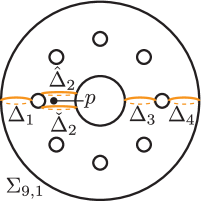
Refer to caption
Figure 17. The curves Δ1,Δ^2,Δˇ2,Δ3,Δ4subscriptΔ1subscript^Δ2subscriptˇΔ2subscriptΔ3subscriptΔ4\Delta_{1},\hat{\Delta}_{2},\check{\Delta}_{2},\Delta_{3},\Delta_{4} on Σ9,1subscriptΣ91\Sigma_{9,1}.

On Σ9subscriptΣ9\Sigma_{9} we take two parallel copies of Δ2subscriptΔ2\Delta_{2}, Δ^2subscript^Δ2\hat{\Delta}_{2} and Δˇ2subscriptˇΔ2\check{\Delta}_{2}, and add a marked point between them as in Figure 17. The first two embeddings Φ1subscriptΦ1\Phi_{1} and Φ2subscriptΦ2\Phi_{2} are now regarded as embeddings of Σ34superscriptsubscriptΣ34\Sigma_{3}^{4} into Σ9,1subscriptΣ91\Sigma_{9,1} in a straightforward fashion, which provide the two relations

t\scaletoa19ptt\scaletoa19ptt\scaletox19ptt\scaletob19ptt\scaletob19ptt\scaletoy19ptt\scaletoc19ptt\scaletoc19ptt\scaletoz19ptt\scaletod19ptt\scaletod19ptt\scaletow19pt=t\scaletoΔ19ptt\scaletoΔ^29ptt\scaletoΔ39ptt\scaletoΔ49pt,subscript𝑡\scaletosubscript𝑎19𝑝𝑡subscript𝑡\scaletosuperscriptsubscript𝑎19𝑝𝑡subscript𝑡\scaletosubscript𝑥19𝑝𝑡subscript𝑡\scaletosubscript𝑏19𝑝𝑡subscript𝑡\scaletosuperscriptsubscript𝑏19𝑝𝑡subscript𝑡\scaletosubscript𝑦19𝑝𝑡subscript𝑡\scaletosubscript𝑐19𝑝𝑡subscript𝑡\scaletosuperscriptsubscript𝑐19𝑝𝑡subscript𝑡\scaletosubscript𝑧19𝑝𝑡subscript𝑡\scaletosubscript𝑑19𝑝𝑡subscript𝑡\scaletosuperscriptsubscript𝑑19𝑝𝑡subscript𝑡\scaletosubscript𝑤19𝑝𝑡subscript𝑡\scaletosubscriptΔ19𝑝𝑡subscript𝑡\scaletosubscript^Δ29𝑝𝑡subscript𝑡\scaletosubscriptΔ39𝑝𝑡subscript𝑡\scaletosubscriptΔ49𝑝𝑡\displaystyle t_{\scaleto{\mathstrut a_{1}}{9pt}}t_{\scaleto{\mathstrut a_{1}^{\prime}}{9pt}}t_{\scaleto{\mathstrut x_{1}}{9pt}}t_{\scaleto{\mathstrut b_{1}}{9pt}}t_{\scaleto{\mathstrut b_{1}^{\prime}}{9pt}}t_{\scaleto{\mathstrut y_{1}}{9pt}}t_{\scaleto{\mathstrut c_{1}}{9pt}}t_{\scaleto{\mathstrut c_{1}^{\prime}}{9pt}}t_{\scaleto{\mathstrut z_{1}}{9pt}}t_{\scaleto{\mathstrut d_{1}}{9pt}}t_{\scaleto{\mathstrut d_{1}^{\prime}}{9pt}}t_{\scaleto{\mathstrut w_{1}}{9pt}}=t_{\scaleto{\mathstrut\Delta_{1}}{9pt}}t_{\scaleto{\mathstrut\hat{\Delta}_{2}}{9pt}}t_{\scaleto{\mathstrut\Delta_{3}}{9pt}}t_{\scaleto{\mathstrut\Delta_{4}}{9pt}},
t\scaletoa29ptt\scaletoa29ptt\scaletox29ptt\scaletob29ptt\scaletob29ptt\scaletoy29ptt\scaletoc29ptt\scaletoc29ptt\scaletoz29ptt\scaletod29ptt\scaletod29ptt\scaletow29pt=t\scaletoΔ19ptt\scaletoΔˇ29ptt\scaletoΔ39ptt\scaletoΔ49ptsubscript𝑡\scaletosubscript𝑎29𝑝𝑡subscript𝑡\scaletosuperscriptsubscript𝑎29𝑝𝑡subscript𝑡\scaletosubscript𝑥29𝑝𝑡subscript𝑡\scaletosubscript𝑏29𝑝𝑡subscript𝑡\scaletosuperscriptsubscript𝑏29𝑝𝑡subscript𝑡\scaletosubscript𝑦29𝑝𝑡subscript𝑡\scaletosubscript𝑐29𝑝𝑡subscript𝑡\scaletosuperscriptsubscript𝑐29𝑝𝑡subscript𝑡\scaletosubscript𝑧29𝑝𝑡subscript𝑡\scaletosubscript𝑑29𝑝𝑡subscript𝑡\scaletosuperscriptsubscript𝑑29𝑝𝑡subscript𝑡\scaletosubscript𝑤29𝑝𝑡subscript𝑡\scaletosubscriptΔ19𝑝𝑡subscript𝑡\scaletosubscriptˇΔ29𝑝𝑡subscript𝑡\scaletosubscriptΔ39𝑝𝑡subscript𝑡\scaletosubscriptΔ49𝑝𝑡\displaystyle t_{\scaleto{\mathstrut a_{2}}{9pt}}t_{\scaleto{\mathstrut a_{2}^{\prime}}{9pt}}t_{\scaleto{\mathstrut x_{2}}{9pt}}t_{\scaleto{\mathstrut b_{2}}{9pt}}t_{\scaleto{\mathstrut b_{2}^{\prime}}{9pt}}t_{\scaleto{\mathstrut y_{2}}{9pt}}t_{\scaleto{\mathstrut c_{2}}{9pt}}t_{\scaleto{\mathstrut c_{2}^{\prime}}{9pt}}t_{\scaleto{\mathstrut z_{2}}{9pt}}t_{\scaleto{\mathstrut d_{2}}{9pt}}t_{\scaleto{\mathstrut d_{2}^{\prime}}{9pt}}t_{\scaleto{\mathstrut w_{2}}{9pt}}=t_{\scaleto{\mathstrut\Delta_{1}}{9pt}}t_{\scaleto{\mathstrut\check{\Delta}_{2}}{9pt}}t_{\scaleto{\mathstrut\Delta_{3}}{9pt}}t_{\scaleto{\mathstrut\Delta_{4}}{9pt}}

in Mod(Σ9,1)ModsubscriptΣ91\operatorname{Mod}(\Sigma_{9,1}). Combining them as before, we get a factorization (with no point-pushing map yet):

(12) t\scaletoa19ptt\scaletoa19ptt\scaletoa29ptt\scaletoa29ptt\scaletoΔ19pt1t\scaletoΔ49pt1¯t\scaletox19ptt\scaletox29ptt\scaletob19ptt\scaletob19ptt\scaletob29ptt\scaletob29ptt\scaletoΔ39pt1t\scaletoΔ49pt1¯t\scaletoy19ptt\scaletoy29pt¯subscript𝑡\scaletosubscript𝑎19𝑝𝑡subscript𝑡\scaletosuperscriptsubscript𝑎19𝑝𝑡subscript𝑡\scaletosubscript𝑎29𝑝𝑡subscript𝑡\scaletosuperscriptsubscript𝑎29𝑝𝑡superscriptsubscript𝑡\scaletosubscriptΔ19𝑝𝑡1superscriptsubscript𝑡\scaletosubscriptΔ49𝑝𝑡1subscript𝑡\scaletosubscript𝑥19𝑝𝑡subscript𝑡\scaletosubscript𝑥29𝑝𝑡¯subscript𝑡\scaletosubscript𝑏19𝑝𝑡subscript𝑡\scaletosuperscriptsubscript𝑏19𝑝𝑡subscript𝑡\scaletosubscript𝑏29𝑝𝑡subscript𝑡\scaletosuperscriptsubscript𝑏29𝑝𝑡superscriptsubscript𝑡\scaletosubscriptΔ39𝑝𝑡1superscriptsubscript𝑡\scaletosubscriptΔ49𝑝𝑡1subscript𝑡\scaletosubscript𝑦19𝑝𝑡subscript𝑡\scaletosubscript𝑦29𝑝𝑡\displaystyle\underline{t_{\scaleto{\mathstrut a_{1}}{9pt}}t_{\scaleto{\mathstrut a_{1}^{\prime}}{9pt}}t_{\scaleto{\mathstrut a_{2}}{9pt}}t_{\scaleto{\mathstrut a_{2}^{\prime}}{9pt}}t_{\scaleto{\mathstrut\Delta_{1}}{9pt}}^{-1}t_{\scaleto{\mathstrut\Delta_{4}}{9pt}}^{-1}}\cdot t_{\scaleto{\mathstrut x_{1}}{9pt}}t_{\scaleto{\mathstrut x_{2}}{9pt}}\cdot\underline{t_{\scaleto{\mathstrut b_{1}}{9pt}}t_{\scaleto{\mathstrut b_{1}^{\prime}}{9pt}}t_{\scaleto{\mathstrut b_{2}}{9pt}}t_{\scaleto{\mathstrut b_{2}^{\prime}}{9pt}}t_{\scaleto{\mathstrut\Delta_{3}}{9pt}}^{-1}t_{\scaleto{\mathstrut\Delta_{4}}{9pt}}^{-1}}\cdot t_{\scaleto{\mathstrut y_{1}}{9pt}}t_{\scaleto{\mathstrut y_{2}}{9pt}}
t\scaletoc19ptt\scaletoc19ptt\scaletoc29ptt\scaletoc29ptt\scaletoΔˇ29pt1t\scaletoΔ39pt1¯t\scaletoz19ptt\scaletoz29ptt\scaletod19ptt\scaletod19ptt\scaletod29ptt\scaletod29ptt\scaletoΔ19pt1t\scaletoΔ^29pt1¯t\scaletow19ptt\scaletow29pt=1.\displaystyle\cdot\underline{t_{\scaleto{\mathstrut c_{1}}{9pt}}t_{\scaleto{\mathstrut c_{1}^{\prime}}{9pt}}t_{\scaleto{\mathstrut c_{2}}{9pt}}t_{\scaleto{\mathstrut c_{2}^{\prime}}{9pt}}t_{\scaleto{\mathstrut\check{\Delta}_{2}}{9pt}}^{-1}t_{\scaleto{\mathstrut\Delta_{3}}{9pt}}^{-1}}\cdot t_{\scaleto{\mathstrut z_{1}}{9pt}}t_{\scaleto{\mathstrut z_{2}}{9pt}}\cdot\underline{t_{\scaleto{\mathstrut d_{1}}{9pt}}t_{\scaleto{\mathstrut d_{1}^{\prime}}{9pt}}t_{\scaleto{\mathstrut d_{2}}{9pt}}t_{\scaleto{\mathstrut d_{2}^{\prime}}{9pt}}t_{\scaleto{\mathstrut\Delta_{1}}{9pt}}^{-1}t_{\scaleto{\mathstrut\hat{\Delta}_{2}}{9pt}}^{-1}}\cdot t_{\scaleto{\mathstrut w_{1}}{9pt}}t_{\scaleto{\mathstrut w_{2}}{9pt}}=1.

We can now describe our embeddings Φ3,Φ4,Φ5,Φ6subscriptΦ3subscriptΦ4subscriptΦ5subscriptΦ6\Phi_{3},\Phi_{4},\Phi_{5},\Phi_{6}. We first modify the presentation of the genus–333 relation (9) so that one of the bounding pair sits in a “standard position” as illustrated in Figure 19. Take the surface Σ3,24superscriptsubscriptΣ324\Sigma_{3,2}^{4} in Figure 13 and slightly slide the boundary components as indicated in Figure 19. Then we conjugate the relation (9) by the series of Dehn twists

t\scaletoβ9ptt\scaletoγ9ptt\scaletoα9ptt\scaletoβ9ptt\scaletoγ9ptt\scaletoα9ptt\scaletoη9pt1subscript𝑡\scaleto𝛽9𝑝𝑡subscript𝑡\scaleto𝛾9𝑝𝑡subscript𝑡\scaleto𝛼9𝑝𝑡subscript𝑡\scaleto𝛽9𝑝𝑡subscript𝑡\scaleto𝛾9𝑝𝑡subscript𝑡\scaleto𝛼9𝑝𝑡superscriptsubscript𝑡\scaleto𝜂9𝑝𝑡1t_{\scaleto{\mathstrut\beta}{9pt}}t_{\scaleto{\mathstrut\gamma}{9pt}}t_{\scaleto{\mathstrut\alpha}{9pt}}t_{\scaleto{\mathstrut\beta}{9pt}}t_{\scaleto{\mathstrut\gamma}{9pt}}t_{\scaleto{\mathstrut\alpha}{9pt}}t_{\scaleto{\mathstrut\eta}{9pt}}^{-1}

with the curves given on the right of Figure 19. This puts the bounding pair d,d𝑑superscript𝑑d,d^{\prime} in the standard position as shown in Figure 19, where the images of the other curves are also given. Here we keep using the same symbols for the curves as those before the conjugation.

[Uncaptioned image]
Figure 18. Sliding the boundary components and the curves for the conjugation.
[Uncaptioned image]
Figure 19. Monodromy curves of the genus–333 pencil with simpler d𝑑d and dsuperscript𝑑d^{\prime}.

By cyclic permutation and commutativity, the relation (9) becomes

(16) 𝒫α2t\scaletow9ptt\scaletoa9ptt\scaletoa9ptt\scaletox9ptt\scaletob9ptt\scaletob9ptt\scaletoy9ptt\scaletoc9ptt\scaletoc9ptt\scaletoz9pt𝒫α1=t\scaletoδ19ptt\scaletoδ29ptt\scaletoδ39ptt\scaletoδ49ptt\scaletod9pt1t\scaletod9pt1.subscript𝒫subscript𝛼2subscript𝑡\scaleto𝑤9𝑝𝑡subscript𝑡\scaleto𝑎9𝑝𝑡subscript𝑡\scaletosuperscript𝑎9𝑝𝑡subscript𝑡\scaleto𝑥9𝑝𝑡subscript𝑡\scaleto𝑏9𝑝𝑡subscript𝑡\scaletosuperscript𝑏9𝑝𝑡subscript𝑡\scaleto𝑦9𝑝𝑡subscript𝑡\scaleto𝑐9𝑝𝑡subscript𝑡\scaletosuperscript𝑐9𝑝𝑡subscript𝑡\scaleto𝑧9𝑝𝑡subscript𝒫subscript𝛼1subscript𝑡\scaletosubscript𝛿19𝑝𝑡subscript𝑡\scaletosubscript𝛿29𝑝𝑡subscript𝑡\scaletosubscript𝛿39𝑝𝑡subscript𝑡\scaletosubscript𝛿49𝑝𝑡superscriptsubscript𝑡\scaleto𝑑9𝑝𝑡1superscriptsubscript𝑡\scaletosuperscript𝑑9𝑝𝑡1\displaystyle\mathcal{P}_{\vec{\alpha}_{2}}\cdot t_{\scaleto{\mathstrut w}{9pt}}t_{\scaleto{\mathstrut a}{9pt}}t_{\scaleto{\mathstrut a^{\prime}}{9pt}}t_{\scaleto{\mathstrut x}{9pt}}t_{\scaleto{\mathstrut b}{9pt}}t_{\scaleto{\mathstrut b^{\prime}}{9pt}}t_{\scaleto{\mathstrut y}{9pt}}t_{\scaleto{\mathstrut c}{9pt}}t_{\scaleto{\mathstrut c^{\prime}}{9pt}}t_{\scaleto{\mathstrut z}{9pt}}\cdot\mathcal{P}_{\vec{\alpha}_{1}}=t_{\scaleto{\mathstrut\delta_{1}}{9pt}}t_{\scaleto{\mathstrut\delta_{2}}{9pt}}t_{\scaleto{\mathstrut\delta_{3}}{9pt}}t_{\scaleto{\mathstrut\delta_{4}}{9pt}}t_{\scaleto{\mathstrut d}{9pt}}^{-1}t_{\scaleto{\mathstrut d^{\prime}}{9pt}}^{-1}.

We will embed the relation (16) with the curves in Figure 19 into Mod(Σ9,1)ModsubscriptΣ91\operatorname{Mod}(\Sigma_{9,1}). For Φ3subscriptΦ3\Phi_{3} and Φ4subscriptΦ4\Phi_{4} we do not need the marked points. For Φ5subscriptΦ5\Phi_{5} we include the marked point p1subscript𝑝1p_{1} and forget p2subscript𝑝2p_{2}, whereas for Φ6subscriptΦ6\Phi_{6} we keep p2subscript𝑝2p_{2} and forget p1subscript𝑝1p_{1}. In Figures 20(a)–(d), we describe the embeddings

Φ3:Σ34Σ9,1,Φ4:Σ34Σ9,1,Φ5:Σ3,14Σ9,1,Φ6:Σ3,14Σ9,1,:subscriptΦ3superscriptsubscriptΣ34subscriptΣ91subscriptΦ4:superscriptsubscriptΣ34subscriptΣ91subscriptΦ5:superscriptsubscriptΣ314subscriptΣ91subscriptΦ6:superscriptsubscriptΣ314subscriptΣ91\displaystyle\Phi_{3}:\Sigma_{3}^{4}\to\Sigma_{9,1},\quad\Phi_{4}:\Sigma_{3}^{4}\to\Sigma_{9,1},\quad\Phi_{5}:\Sigma_{3,1}^{4}\to\Sigma_{9,1},\quad\Phi_{6}:\Sigma_{3,1}^{4}\to\Sigma_{9,1},

as the compositions of embeddings Φ~isubscript~Φ𝑖\tilde{\Phi}_{i} (which are easier to visualize) and diffeomorphisms ψisubscript𝜓𝑖\psi_{i} of Σ9,1subscriptΣ91\Sigma_{9,1}. The embeddings Φ~isubscript~Φ𝑖\tilde{\Phi}_{i} are uniquely specified by describing how the gray curves that fill the genus–333 surfaces are embedded. The diffeomorphisms ψ3,ψ4,ψ5subscript𝜓3subscript𝜓4subscript𝜓5\psi_{3},\psi_{4},\psi_{5} and ψ6subscript𝜓6\psi_{6}, are given by the products of Dehn twists below. Here tisubscript𝑡𝑖t_{i} means the right-handed Dehn twist along the curve labeled i𝑖i in the respective Figures 21(a)–(d):

ψ3subscript𝜓3\displaystyle\psi_{3} :=t4ˇ1t4^1t3ˇ1t3^1t2ˇ1t2^1t1ˇ1t1^1,assignabsentsuperscriptsubscript𝑡ˇ41superscriptsubscript𝑡^41superscriptsubscript𝑡ˇ31superscriptsubscript𝑡^31superscriptsubscript𝑡ˇ21superscriptsubscript𝑡^21superscriptsubscript𝑡ˇ11superscriptsubscript𝑡^11\displaystyle:=t_{\check{4}}^{-1}t_{\hat{4}}^{-1}t_{\check{3}}^{-1}t_{\hat{3}}^{-1}t_{\check{2}}^{-1}t_{\hat{2}}^{-1}t_{\check{1}}^{-1}t_{\hat{1}}^{-1},
ψ4subscript𝜓4\displaystyle\psi_{4} :=t112t10ˇt10^t9ˇ1t9^1t8ˇ1t8^1t5ˇ1t5^1t4ˇ1t4^1t7ˇ1t7^1t6ˇ1t6^1assignabsentsuperscriptsubscript𝑡112subscript𝑡ˇ10subscript𝑡^10superscriptsubscript𝑡ˇ91superscriptsubscript𝑡^91superscriptsubscript𝑡ˇ81superscriptsubscript𝑡^81superscriptsubscript𝑡ˇ51superscriptsubscript𝑡^51superscriptsubscript𝑡ˇ41superscriptsubscript𝑡^41superscriptsubscript𝑡ˇ71superscriptsubscript𝑡^71superscriptsubscript𝑡ˇ61superscriptsubscript𝑡^61\displaystyle:=t_{11}^{2}t_{\check{10}}t_{\hat{10}}t_{\check{9}}^{-1}t_{\hat{9}}^{-1}t_{\check{8}}^{-1}t_{\hat{8}}^{-1}t_{\check{5}}^{-1}t_{\hat{5}}^{-1}t_{\check{4}}^{-1}t_{\hat{4}}^{-1}t_{\check{7}}^{-1}t_{\hat{7}}^{-1}t_{\check{6}}^{-1}t_{\hat{6}}^{-1}
t3ˇ1t3^1t2ˇ1t2^1t1ˇ1t1^1t5ˇ1t5^1t4ˇ1t4^1t3ˇ1t3^1t2ˇ1t2^1t1ˇ1t1^1,absentsuperscriptsubscript𝑡ˇ31superscriptsubscript𝑡^31superscriptsubscript𝑡ˇ21superscriptsubscript𝑡^21superscriptsubscript𝑡ˇ11superscriptsubscript𝑡^11superscriptsubscript𝑡ˇ51superscriptsubscript𝑡^51superscriptsubscript𝑡ˇ41superscriptsubscript𝑡^41superscriptsubscript𝑡ˇ31superscriptsubscript𝑡^31superscriptsubscript𝑡ˇ21superscriptsubscript𝑡^21superscriptsubscript𝑡ˇ11superscriptsubscript𝑡^11\displaystyle\qquad\cdot t_{\check{3}}^{-1}t_{\hat{3}}^{-1}t_{\check{2}}^{-1}t_{\hat{2}}^{-1}t_{\check{1}}^{-1}t_{\hat{1}}^{-1}t_{\check{5}}^{-1}t_{\hat{5}}^{-1}t_{\check{4}}^{-1}t_{\hat{4}}^{-1}t_{\check{3}}^{-1}t_{\hat{3}}^{-1}t_{\check{2}}^{-1}t_{\hat{2}}^{-1}t_{\check{1}}^{-1}t_{\hat{1}}^{-1},
ψ5subscript𝜓5\displaystyle\psi_{5} :=t4ˇt4^t3ˇt3^t2ˇt2^t1ˇt1^,assignabsentsubscript𝑡ˇ4subscript𝑡^4subscript𝑡ˇ3subscript𝑡^3subscript𝑡ˇ2subscript𝑡^2subscript𝑡ˇ1subscript𝑡^1\displaystyle:=t_{\check{4}}t_{\hat{4}}t_{\check{3}}t_{\hat{3}}t_{\check{2}}t_{\hat{2}}t_{\check{1}}t_{\hat{1}},
ψ6subscript𝜓6\displaystyle\psi_{6} :=t6ˇ1t6^1t5ˇt5^t4ˇt4^t3ˇ1t3^1t2ˇ1t2^1t1ˇ1t1^1t3ˇ1t3^1t2ˇ1t2^1t1ˇ1t1^1.assignabsentsuperscriptsubscript𝑡ˇ61superscriptsubscript𝑡^61subscript𝑡ˇ5subscript𝑡^5subscript𝑡ˇ4subscript𝑡^4superscriptsubscript𝑡ˇ31superscriptsubscript𝑡^31superscriptsubscript𝑡ˇ21superscriptsubscript𝑡^21superscriptsubscript𝑡ˇ11superscriptsubscript𝑡^11superscriptsubscript𝑡ˇ31superscriptsubscript𝑡^31superscriptsubscript𝑡ˇ21superscriptsubscript𝑡^21superscriptsubscript𝑡ˇ11superscriptsubscript𝑡^11\displaystyle:=t_{\check{6}}^{-1}t_{\hat{6}}^{-1}t_{\check{5}}t_{\hat{5}}t_{\check{4}}t_{\hat{4}}t_{\check{3}}^{-1}t_{\hat{3}}^{-1}t_{\check{2}}^{-1}t_{\hat{2}}^{-1}t_{\check{1}}^{-1}t_{\hat{1}}^{-1}t_{\check{3}}^{-1}t_{\hat{3}}^{-1}t_{\check{2}}^{-1}t_{\hat{2}}^{-1}t_{\check{1}}^{-1}t_{\hat{1}}^{-1}.
Refer to caption
(a) The embedding Φ3=ψ3Φ~3subscriptΦ3subscript𝜓3subscript~Φ3\Phi_{3}=\psi_{3}\circ\tilde{\Phi}_{3}.
Refer to caption
(b) The embedding Φ4=ψ4Φ~4subscriptΦ4subscript𝜓4subscript~Φ4\Phi_{4}=\psi_{4}\circ\tilde{\Phi}_{4}.
Refer to caption
(c) The embedding Φ5=ψ5Φ~5subscriptΦ5subscript𝜓5subscript~Φ5\Phi_{5}=\psi_{5}\circ\tilde{\Phi}_{5}.
Refer to caption
(d) The embedding Φ6=ψ6Φ~6subscriptΦ6subscript𝜓6subscript~Φ6\Phi_{6}=\psi_{6}\circ\tilde{\Phi}_{6}.
Figure 20. The embeddings.
Refer to caption
(a) Curves for ψ3subscript𝜓3\psi_{3}
Refer to caption
(b) for ψ4subscript𝜓4\psi_{4}
Refer to caption
(c) for ψ5subscript𝜓5\psi_{5}
Refer to caption
(d) for ψ6subscript𝜓6\psi_{6}
Figure 21. Dehn twist curves for the diffeomorphisms ψ3,ψ4,ψ5,ψ6subscript𝜓3subscript𝜓4subscript𝜓5subscript𝜓6\psi_{3},\psi_{4},\psi_{5},\psi_{6}.

So we have

  • Φ3subscriptΦ3\Phi_{3} maps (δ1,δ2,δ3,δ4,d,d)subscript𝛿1subscript𝛿2subscript𝛿3subscript𝛿4𝑑superscript𝑑(\delta_{1},\delta_{2},\delta_{3},\delta_{4},d,d^{\prime}) to (a1,a1,a2,a2,Δ4,Δ1)subscript𝑎1superscriptsubscript𝑎1superscriptsubscript𝑎2subscript𝑎2subscriptΔ4subscriptΔ1(a_{1},a_{1}^{\prime},a_{2}^{\prime},a_{2},\Delta_{4},\Delta_{1}),

  • Φ4subscriptΦ4\Phi_{4} maps (δ1,δ2,δ3,δ4,d,d)subscript𝛿1subscript𝛿2subscript𝛿3subscript𝛿4𝑑superscript𝑑(\delta_{1},\delta_{2},\delta_{3},\delta_{4},d,d^{\prime}) to (b1,b1,b2,b2,Δ4,Δ3)subscript𝑏1superscriptsubscript𝑏1subscript𝑏2superscriptsubscript𝑏2subscriptΔ4subscriptΔ3(b_{1},b_{1}^{\prime},b_{2},b_{2}^{\prime},\Delta_{4},\Delta_{3}),

  • Φ5subscriptΦ5\Phi_{5} maps (δ1,δ2,δ3,δ4,d,d)subscript𝛿1subscript𝛿2subscript𝛿3subscript𝛿4𝑑superscript𝑑(\delta_{1},\delta_{2},\delta_{3},\delta_{4},d,d^{\prime}) to (c1,c1,c2,c2,Δ3,Δˇ2)subscript𝑐1superscriptsubscript𝑐1superscriptsubscript𝑐2subscript𝑐2subscriptΔ3subscriptˇΔ2(c_{1},c_{1}^{\prime},c_{2}^{\prime},c_{2},\Delta_{3},\check{\Delta}_{2}),

  • Φ6subscriptΦ6\Phi_{6} maps (δ1,δ2,δ3,δ4,d,d)subscript𝛿1subscript𝛿2subscript𝛿3subscript𝛿4𝑑superscript𝑑(\delta_{1},\delta_{2},\delta_{3},\delta_{4},d,d^{\prime}) to (d1,d1,d2,d2,Δ^2,Δ1)subscript𝑑1superscriptsubscript𝑑1subscript𝑑2superscriptsubscript𝑑2subscript^Δ2subscriptΔ1(d_{1},d_{1}^{\prime},d_{2},d_{2}^{\prime},\hat{\Delta}_{2},\Delta_{1}).

Under these embeddings, the modified genus–333 relation (16) yields

t\scaletow39ptt\scaletoa39ptt\scaletoa39ptt\scaletox39ptt\scaletob39ptt\scaletob39ptt\scaletoy39ptt\scaletoc39ptt\scaletoc39ptt\scaletoz39ptsubscript𝑡\scaletosubscript𝑤39𝑝𝑡subscript𝑡\scaletosubscript𝑎39𝑝𝑡subscript𝑡\scaletosuperscriptsubscript𝑎39𝑝𝑡subscript𝑡\scaletosubscript𝑥39𝑝𝑡subscript𝑡\scaletosubscript𝑏39𝑝𝑡subscript𝑡\scaletosuperscriptsubscript𝑏39𝑝𝑡subscript𝑡\scaletosubscript𝑦39𝑝𝑡subscript𝑡\scaletosubscript𝑐39𝑝𝑡subscript𝑡\scaletosuperscriptsubscript𝑐39𝑝𝑡subscript𝑡\scaletosubscript𝑧39𝑝𝑡\displaystyle t_{\scaleto{\mathstrut w_{3}}{9pt}}t_{\scaleto{\mathstrut a_{3}}{9pt}}t_{\scaleto{\mathstrut a_{3}^{\prime}}{9pt}}t_{\scaleto{\mathstrut x_{3}}{9pt}}t_{\scaleto{\mathstrut b_{3}}{9pt}}t_{\scaleto{\mathstrut b_{3}^{\prime}}{9pt}}t_{\scaleto{\mathstrut y_{3}}{9pt}}t_{\scaleto{\mathstrut c_{3}}{9pt}}t_{\scaleto{\mathstrut c_{3}^{\prime}}{9pt}}t_{\scaleto{\mathstrut z_{3}}{9pt}} =t\scaletoa19ptt\scaletoa19ptt\scaletoa29ptt\scaletoa29ptt\scaletoΔ19pt1t\scaletoΔ49pt1,absentsubscript𝑡\scaletosubscript𝑎19𝑝𝑡subscript𝑡\scaletosuperscriptsubscript𝑎19𝑝𝑡subscript𝑡\scaletosubscript𝑎29𝑝𝑡subscript𝑡\scaletosuperscriptsubscript𝑎29𝑝𝑡superscriptsubscript𝑡\scaletosubscriptΔ19𝑝𝑡1superscriptsubscript𝑡\scaletosubscriptΔ49𝑝𝑡1\displaystyle=t_{\scaleto{\mathstrut a_{1}}{9pt}}t_{\scaleto{\mathstrut a_{1}^{\prime}}{9pt}}t_{\scaleto{\mathstrut a_{2}}{9pt}}t_{\scaleto{\mathstrut a_{2}^{\prime}}{9pt}}t_{\scaleto{\mathstrut\Delta_{1}}{9pt}}^{-1}t_{\scaleto{\mathstrut\Delta_{4}}{9pt}}^{-1},
t\scaletow49ptt\scaletoa49ptt\scaletoa49ptt\scaletox49ptt\scaletob49ptt\scaletob49ptt\scaletoy49ptt\scaletoc49ptt\scaletoc49ptt\scaletoz49ptsubscript𝑡\scaletosubscript𝑤49𝑝𝑡subscript𝑡\scaletosubscript𝑎49𝑝𝑡subscript𝑡\scaletosuperscriptsubscript𝑎49𝑝𝑡subscript𝑡\scaletosubscript𝑥49𝑝𝑡subscript𝑡\scaletosubscript𝑏49𝑝𝑡subscript𝑡\scaletosuperscriptsubscript𝑏49𝑝𝑡subscript𝑡\scaletosubscript𝑦49𝑝𝑡subscript𝑡\scaletosubscript𝑐49𝑝𝑡subscript𝑡\scaletosuperscriptsubscript𝑐49𝑝𝑡subscript𝑡\scaletosubscript𝑧49𝑝𝑡\displaystyle t_{\scaleto{\mathstrut w_{4}}{9pt}}t_{\scaleto{\mathstrut a_{4}}{9pt}}t_{\scaleto{\mathstrut a_{4}^{\prime}}{9pt}}t_{\scaleto{\mathstrut x_{4}}{9pt}}t_{\scaleto{\mathstrut b_{4}}{9pt}}t_{\scaleto{\mathstrut b_{4}^{\prime}}{9pt}}t_{\scaleto{\mathstrut y_{4}}{9pt}}t_{\scaleto{\mathstrut c_{4}}{9pt}}t_{\scaleto{\mathstrut c_{4}^{\prime}}{9pt}}t_{\scaleto{\mathstrut z_{4}}{9pt}} =t\scaletob19ptt\scaletob19ptt\scaletob29ptt\scaletob29ptt\scaletoΔ39pt1t\scaletoΔ49pt1,absentsubscript𝑡\scaletosubscript𝑏19𝑝𝑡subscript𝑡\scaletosuperscriptsubscript𝑏19𝑝𝑡subscript𝑡\scaletosubscript𝑏29𝑝𝑡subscript𝑡\scaletosuperscriptsubscript𝑏29𝑝𝑡superscriptsubscript𝑡\scaletosubscriptΔ39𝑝𝑡1superscriptsubscript𝑡\scaletosubscriptΔ49𝑝𝑡1\displaystyle=t_{\scaleto{\mathstrut b_{1}}{9pt}}t_{\scaleto{\mathstrut b_{1}^{\prime}}{9pt}}t_{\scaleto{\mathstrut b_{2}}{9pt}}t_{\scaleto{\mathstrut b_{2}^{\prime}}{9pt}}t_{\scaleto{\mathstrut\Delta_{3}}{9pt}}^{-1}t_{\scaleto{\mathstrut\Delta_{4}}{9pt}}^{-1},
t\scaletow59ptt\scaletoa59ptt\scaletoa59ptt\scaletox59ptt\scaletob59ptt\scaletob59ptt\scaletoy59ptt\scaletoc59ptt\scaletoc59ptt\scaletoz59pt𝒫α1subscript𝑡\scaletosubscript𝑤59𝑝𝑡subscript𝑡\scaletosubscript𝑎59𝑝𝑡subscript𝑡\scaletosuperscriptsubscript𝑎59𝑝𝑡subscript𝑡\scaletosubscript𝑥59𝑝𝑡subscript𝑡\scaletosubscript𝑏59𝑝𝑡subscript𝑡\scaletosuperscriptsubscript𝑏59𝑝𝑡subscript𝑡\scaletosubscript𝑦59𝑝𝑡subscript𝑡\scaletosubscript𝑐59𝑝𝑡subscript𝑡\scaletosuperscriptsubscript𝑐59𝑝𝑡subscript𝑡\scaletosubscript𝑧59𝑝𝑡subscript𝒫subscript𝛼1\displaystyle t_{\scaleto{\mathstrut w_{5}}{9pt}}t_{\scaleto{\mathstrut a_{5}}{9pt}}t_{\scaleto{\mathstrut a_{5}^{\prime}}{9pt}}t_{\scaleto{\mathstrut x_{5}}{9pt}}t_{\scaleto{\mathstrut b_{5}}{9pt}}t_{\scaleto{\mathstrut b_{5}^{\prime}}{9pt}}t_{\scaleto{\mathstrut y_{5}}{9pt}}t_{\scaleto{\mathstrut c_{5}}{9pt}}t_{\scaleto{\mathstrut c_{5}^{\prime}}{9pt}}t_{\scaleto{\mathstrut z_{5}}{9pt}}\cdot\mathcal{P}_{\vec{\alpha}_{1}} =t\scaletoc19ptt\scaletoc19ptt\scaletoc29ptt\scaletoc29ptt\scaletoΔˇ29pt1t\scaletoΔ39pt1,absentsubscript𝑡\scaletosubscript𝑐19𝑝𝑡subscript𝑡\scaletosuperscriptsubscript𝑐19𝑝𝑡subscript𝑡\scaletosubscript𝑐29𝑝𝑡subscript𝑡\scaletosuperscriptsubscript𝑐29𝑝𝑡superscriptsubscript𝑡\scaletosubscriptˇΔ29𝑝𝑡1superscriptsubscript𝑡\scaletosubscriptΔ39𝑝𝑡1\displaystyle=t_{\scaleto{\mathstrut c_{1}}{9pt}}t_{\scaleto{\mathstrut c_{1}^{\prime}}{9pt}}t_{\scaleto{\mathstrut c_{2}}{9pt}}t_{\scaleto{\mathstrut c_{2}^{\prime}}{9pt}}t_{\scaleto{\mathstrut\check{\Delta}_{2}}{9pt}}^{-1}t_{\scaleto{\mathstrut\Delta_{3}}{9pt}}^{-1},
𝒫α2t\scaletow69ptt\scaletoa69ptt\scaletoa69ptt\scaletox69ptt\scaletob69ptt\scaletob69ptt\scaletoy69ptt\scaletoc69ptt\scaletoc69ptt\scaletoz69ptsubscript𝒫subscript𝛼2subscript𝑡\scaletosubscript𝑤69𝑝𝑡subscript𝑡\scaletosubscript𝑎69𝑝𝑡subscript𝑡\scaletosuperscriptsubscript𝑎69𝑝𝑡subscript𝑡\scaletosubscript𝑥69𝑝𝑡subscript𝑡\scaletosubscript𝑏69𝑝𝑡subscript𝑡\scaletosuperscriptsubscript𝑏69𝑝𝑡subscript𝑡\scaletosubscript𝑦69𝑝𝑡subscript𝑡\scaletosubscript𝑐69𝑝𝑡subscript𝑡\scaletosuperscriptsubscript𝑐69𝑝𝑡subscript𝑡\scaletosubscript𝑧69𝑝𝑡\displaystyle\mathcal{P}_{\vec{\alpha}_{2}}\cdot t_{\scaleto{\mathstrut w_{6}}{9pt}}t_{\scaleto{\mathstrut a_{6}}{9pt}}t_{\scaleto{\mathstrut a_{6}^{\prime}}{9pt}}t_{\scaleto{\mathstrut x_{6}}{9pt}}t_{\scaleto{\mathstrut b_{6}}{9pt}}t_{\scaleto{\mathstrut b_{6}^{\prime}}{9pt}}t_{\scaleto{\mathstrut y_{6}}{9pt}}t_{\scaleto{\mathstrut c_{6}}{9pt}}t_{\scaleto{\mathstrut c_{6}^{\prime}}{9pt}}t_{\scaleto{\mathstrut z_{6}}{9pt}} =t\scaletod19ptt\scaletod19ptt\scaletod29ptt\scaletod29ptt\scaletoΔ19pt1t\scaletoΔ^29pt1.absentsubscript𝑡\scaletosubscript𝑑19𝑝𝑡subscript𝑡\scaletosuperscriptsubscript𝑑19𝑝𝑡subscript𝑡\scaletosubscript𝑑29𝑝𝑡subscript𝑡\scaletosuperscriptsubscript𝑑29𝑝𝑡superscriptsubscript𝑡\scaletosubscriptΔ19𝑝𝑡1superscriptsubscript𝑡\scaletosubscript^Δ29𝑝𝑡1\displaystyle=t_{\scaleto{\mathstrut d_{1}}{9pt}}t_{\scaleto{\mathstrut d_{1}^{\prime}}{9pt}}t_{\scaleto{\mathstrut d_{2}}{9pt}}t_{\scaleto{\mathstrut d_{2}^{\prime}}{9pt}}t_{\scaleto{\mathstrut\Delta_{1}}{9pt}}^{-1}t_{\scaleto{\mathstrut\hat{\Delta}_{2}}{9pt}}^{-1}.

The images of the curves under these embeddings are given in Figures 23. In addition, the oriented loops α1,α2subscript𝛼1subscript𝛼2\vec{\alpha}_{1},\vec{\alpha}_{2} for the point-pushing maps are given in Figure 22. By substituting all into the relation (12), we get

t\scaletow39ptt\scaletoa39ptt\scaletoa39ptt\scaletox39ptt\scaletob39ptt\scaletob39ptt\scaletoy39ptt\scaletoc39ptt\scaletoc39ptt\scaletoz39ptt\scaletox19ptt\scaletox29ptt\scaletow49ptt\scaletoa49ptt\scaletoa49ptt\scaletox49ptt\scaletob49ptt\scaletob49ptt\scaletoy49ptt\scaletoc49ptt\scaletoc49ptt\scaletoz49ptt\scaletoy19ptt\scaletoy29ptsubscript𝑡\scaletosubscript𝑤39𝑝𝑡subscript𝑡\scaletosubscript𝑎39𝑝𝑡subscript𝑡\scaletosuperscriptsubscript𝑎39𝑝𝑡subscript𝑡\scaletosubscript𝑥39𝑝𝑡subscript𝑡\scaletosubscript𝑏39𝑝𝑡subscript𝑡\scaletosuperscriptsubscript𝑏39𝑝𝑡subscript𝑡\scaletosubscript𝑦39𝑝𝑡subscript𝑡\scaletosubscript𝑐39𝑝𝑡subscript𝑡\scaletosuperscriptsubscript𝑐39𝑝𝑡subscript𝑡\scaletosubscript𝑧39𝑝𝑡subscript𝑡\scaletosubscript𝑥19𝑝𝑡subscript𝑡\scaletosubscript𝑥29𝑝𝑡subscript𝑡\scaletosubscript𝑤49𝑝𝑡subscript𝑡\scaletosubscript𝑎49𝑝𝑡subscript𝑡\scaletosuperscriptsubscript𝑎49𝑝𝑡subscript𝑡\scaletosubscript𝑥49𝑝𝑡subscript𝑡\scaletosubscript𝑏49𝑝𝑡subscript𝑡\scaletosuperscriptsubscript𝑏49𝑝𝑡subscript𝑡\scaletosubscript𝑦49𝑝𝑡subscript𝑡\scaletosubscript𝑐49𝑝𝑡subscript𝑡\scaletosuperscriptsubscript𝑐49𝑝𝑡subscript𝑡\scaletosubscript𝑧49𝑝𝑡subscript𝑡\scaletosubscript𝑦19𝑝𝑡subscript𝑡\scaletosubscript𝑦29𝑝𝑡\displaystyle t_{\scaleto{\mathstrut w_{3}}{9pt}}t_{\scaleto{\mathstrut a_{3}}{9pt}}t_{\scaleto{\mathstrut a_{3}^{\prime}}{9pt}}t_{\scaleto{\mathstrut x_{3}}{9pt}}t_{\scaleto{\mathstrut b_{3}}{9pt}}t_{\scaleto{\mathstrut b_{3}^{\prime}}{9pt}}t_{\scaleto{\mathstrut y_{3}}{9pt}}t_{\scaleto{\mathstrut c_{3}}{9pt}}t_{\scaleto{\mathstrut c_{3}^{\prime}}{9pt}}t_{\scaleto{\mathstrut z_{3}}{9pt}}t_{\scaleto{\mathstrut x_{1}}{9pt}}t_{\scaleto{\mathstrut x_{2}}{9pt}}\cdot t_{\scaleto{\mathstrut w_{4}}{9pt}}t_{\scaleto{\mathstrut a_{4}}{9pt}}t_{\scaleto{\mathstrut a_{4}^{\prime}}{9pt}}t_{\scaleto{\mathstrut x_{4}}{9pt}}t_{\scaleto{\mathstrut b_{4}}{9pt}}t_{\scaleto{\mathstrut b_{4}^{\prime}}{9pt}}t_{\scaleto{\mathstrut y_{4}}{9pt}}t_{\scaleto{\mathstrut c_{4}}{9pt}}t_{\scaleto{\mathstrut c_{4}^{\prime}}{9pt}}t_{\scaleto{\mathstrut z_{4}}{9pt}}t_{\scaleto{\mathstrut y_{1}}{9pt}}t_{\scaleto{\mathstrut y_{2}}{9pt}}
t\scaletow59ptt\scaletoa59ptt\scaletoa59ptt\scaletox59ptt\scaletob59ptt\scaletob59ptt\scaletoy59ptt\scaletoc59ptt\scaletoc59ptt\scaletoz59pt𝒫α1t\scaletoz19ptt\scaletoz29pt𝒫α2¯t\scaletow69ptt\scaletoa69ptt\scaletoa69ptt\scaletox69ptt\scaletob69ptt\scaletob69ptt\scaletoy69ptt\scaletoc69ptt\scaletoc69ptt\scaletoz69ptt\scaletow19ptt\scaletow29pt=1.\displaystyle\cdot t_{\scaleto{\mathstrut w_{5}}{9pt}}t_{\scaleto{\mathstrut a_{5}}{9pt}}t_{\scaleto{\mathstrut a_{5}^{\prime}}{9pt}}t_{\scaleto{\mathstrut x_{5}}{9pt}}t_{\scaleto{\mathstrut b_{5}}{9pt}}t_{\scaleto{\mathstrut b_{5}^{\prime}}{9pt}}t_{\scaleto{\mathstrut y_{5}}{9pt}}t_{\scaleto{\mathstrut c_{5}}{9pt}}t_{\scaleto{\mathstrut c_{5}^{\prime}}{9pt}}t_{\scaleto{\mathstrut z_{5}}{9pt}}\cdot\underline{\mathcal{P}_{\vec{\alpha}_{1}}\cdot t_{\scaleto{\mathstrut z_{1}}{9pt}}t_{\scaleto{\mathstrut z_{2}}{9pt}}\cdot\mathcal{P}_{\vec{\alpha}_{2}}}\cdot t_{\scaleto{\mathstrut w_{6}}{9pt}}t_{\scaleto{\mathstrut a_{6}}{9pt}}t_{\scaleto{\mathstrut a_{6}^{\prime}}{9pt}}t_{\scaleto{\mathstrut x_{6}}{9pt}}t_{\scaleto{\mathstrut b_{6}}{9pt}}t_{\scaleto{\mathstrut b_{6}^{\prime}}{9pt}}t_{\scaleto{\mathstrut y_{6}}{9pt}}t_{\scaleto{\mathstrut c_{6}}{9pt}}t_{\scaleto{\mathstrut c_{6}^{\prime}}{9pt}}t_{\scaleto{\mathstrut z_{6}}{9pt}}t_{\scaleto{\mathstrut w_{1}}{9pt}}t_{\scaleto{\mathstrut w_{2}}{9pt}}=1.

Here z1subscript𝑧1z_{1} and z2subscript𝑧2z_{2} are disjoint, α1subscript𝛼1\vec{\alpha}_{1} and z2subscript𝑧2z_{2} are disjoint, and z1subscript𝑧1z_{1} and α2subscript𝛼2\vec{\alpha}_{2} are disjoint, so we get

𝒫α1t\scaletoz19ptt\scaletoz29pt𝒫α2=𝒫α1t\scaletoz29ptt\scaletoz19pt𝒫α2=t\scaletoz29pt𝒫α1𝒫α2t\scaletoz19pt.subscript𝒫subscript𝛼1subscript𝑡\scaletosubscript𝑧19𝑝𝑡subscript𝑡\scaletosubscript𝑧29𝑝𝑡subscript𝒫subscript𝛼2subscript𝒫subscript𝛼1subscript𝑡\scaletosubscript𝑧29𝑝𝑡subscript𝑡\scaletosubscript𝑧19𝑝𝑡subscript𝒫subscript𝛼2subscript𝑡\scaletosubscript𝑧29𝑝𝑡subscript𝒫subscript𝛼1subscript𝒫subscript𝛼2subscript𝑡\scaletosubscript𝑧19𝑝𝑡\displaystyle\mathcal{P}_{\vec{\alpha}_{1}}\cdot t_{\scaleto{\mathstrut z_{1}}{9pt}}t_{\scaleto{\mathstrut z_{2}}{9pt}}\cdot\mathcal{P}_{\vec{\alpha}_{2}}=\mathcal{P}_{\vec{\alpha}_{1}}\cdot t_{\scaleto{\mathstrut z_{2}}{9pt}}t_{\scaleto{\mathstrut z_{1}}{9pt}}\cdot\mathcal{P}_{\vec{\alpha}_{2}}=t_{\scaleto{\mathstrut z_{2}}{9pt}}\cdot\mathcal{P}_{\vec{\alpha}_{1}}\mathcal{P}_{\vec{\alpha}_{2}}\cdot t_{\scaleto{\mathstrut z_{1}}{9pt}}.

Then the product 𝒫α1𝒫α2subscript𝒫subscript𝛼1subscript𝒫subscript𝛼2\mathcal{P}_{\vec{\alpha}_{1}}\mathcal{P}_{\vec{\alpha}_{2}} is equal to the single point-pushing map along α𝛼\vec{\alpha}, which is homotopic to the concatenation α2α1subscript𝛼2subscript𝛼1\vec{\alpha}_{2}\cdot\vec{\alpha}_{1}.

Refer to caption
Figure 22. Curves of the point-pushing maps.

Hence, we obtain the factorization in Mod(Σ9,1)ModsubscriptΣ91\operatorname{Mod}(\Sigma_{9,1}):

(17) t\scaletow39ptt\scaletoa39ptt\scaletoa39ptt\scaletox39ptt\scaletob39ptt\scaletob39ptt\scaletoy39ptt\scaletoc39ptt\scaletoc39ptt\scaletoz39ptt\scaletox19ptt\scaletox29ptt\scaletow49ptt\scaletoa49ptt\scaletoa49ptt\scaletox49ptt\scaletob49ptt\scaletob49ptt\scaletoy49ptt\scaletoc49ptt\scaletoc49ptt\scaletoz49ptt\scaletoy19ptt\scaletoy29ptsubscript𝑡\scaletosubscript𝑤39𝑝𝑡subscript𝑡\scaletosubscript𝑎39𝑝𝑡subscript𝑡\scaletosuperscriptsubscript𝑎39𝑝𝑡subscript𝑡\scaletosubscript𝑥39𝑝𝑡subscript𝑡\scaletosubscript𝑏39𝑝𝑡subscript𝑡\scaletosuperscriptsubscript𝑏39𝑝𝑡subscript𝑡\scaletosubscript𝑦39𝑝𝑡subscript𝑡\scaletosubscript𝑐39𝑝𝑡subscript𝑡\scaletosuperscriptsubscript𝑐39𝑝𝑡subscript𝑡\scaletosubscript𝑧39𝑝𝑡subscript𝑡\scaletosubscript𝑥19𝑝𝑡subscript𝑡\scaletosubscript𝑥29𝑝𝑡subscript𝑡\scaletosubscript𝑤49𝑝𝑡subscript𝑡\scaletosubscript𝑎49𝑝𝑡subscript𝑡\scaletosuperscriptsubscript𝑎49𝑝𝑡subscript𝑡\scaletosubscript𝑥49𝑝𝑡subscript𝑡\scaletosubscript𝑏49𝑝𝑡subscript𝑡\scaletosuperscriptsubscript𝑏49𝑝𝑡subscript𝑡\scaletosubscript𝑦49𝑝𝑡subscript𝑡\scaletosubscript𝑐49𝑝𝑡subscript𝑡\scaletosuperscriptsubscript𝑐49𝑝𝑡subscript𝑡\scaletosubscript𝑧49𝑝𝑡subscript𝑡\scaletosubscript𝑦19𝑝𝑡subscript𝑡\scaletosubscript𝑦29𝑝𝑡\displaystyle t_{\scaleto{\mathstrut w_{3}}{9pt}}t_{\scaleto{\mathstrut a_{3}}{9pt}}t_{\scaleto{\mathstrut a_{3}^{\prime}}{9pt}}t_{\scaleto{\mathstrut x_{3}}{9pt}}t_{\scaleto{\mathstrut b_{3}}{9pt}}t_{\scaleto{\mathstrut b_{3}^{\prime}}{9pt}}t_{\scaleto{\mathstrut y_{3}}{9pt}}t_{\scaleto{\mathstrut c_{3}}{9pt}}t_{\scaleto{\mathstrut c_{3}^{\prime}}{9pt}}t_{\scaleto{\mathstrut z_{3}}{9pt}}t_{\scaleto{\mathstrut x_{1}}{9pt}}t_{\scaleto{\mathstrut x_{2}}{9pt}}\cdot t_{\scaleto{\mathstrut w_{4}}{9pt}}t_{\scaleto{\mathstrut a_{4}}{9pt}}t_{\scaleto{\mathstrut a_{4}^{\prime}}{9pt}}t_{\scaleto{\mathstrut x_{4}}{9pt}}t_{\scaleto{\mathstrut b_{4}}{9pt}}t_{\scaleto{\mathstrut b_{4}^{\prime}}{9pt}}t_{\scaleto{\mathstrut y_{4}}{9pt}}t_{\scaleto{\mathstrut c_{4}}{9pt}}t_{\scaleto{\mathstrut c_{4}^{\prime}}{9pt}}t_{\scaleto{\mathstrut z_{4}}{9pt}}t_{\scaleto{\mathstrut y_{1}}{9pt}}t_{\scaleto{\mathstrut y_{2}}{9pt}}
t\scaletow59ptt\scaletoa59ptt\scaletoa59ptt\scaletox59ptt\scaletob59ptt\scaletob59ptt\scaletoy59ptt\scaletoc59ptt\scaletoc59ptt\scaletoz59ptt\scaletoz29pt𝒫αt\scaletoz19ptt\scaletow69ptt\scaletoa69ptt\scaletoa69ptt\scaletox69ptt\scaletob69ptt\scaletob69ptt\scaletoy69ptt\scaletoc69ptt\scaletoc69ptt\scaletoz69ptt\scaletow19ptt\scaletow29ptabsentsubscript𝑡\scaletosubscript𝑤59𝑝𝑡subscript𝑡\scaletosubscript𝑎59𝑝𝑡subscript𝑡\scaletosuperscriptsubscript𝑎59𝑝𝑡subscript𝑡\scaletosubscript𝑥59𝑝𝑡subscript𝑡\scaletosubscript𝑏59𝑝𝑡subscript𝑡\scaletosuperscriptsubscript𝑏59𝑝𝑡subscript𝑡\scaletosubscript𝑦59𝑝𝑡subscript𝑡\scaletosubscript𝑐59𝑝𝑡subscript𝑡\scaletosuperscriptsubscript𝑐59𝑝𝑡subscript𝑡\scaletosubscript𝑧59𝑝𝑡subscript𝑡\scaletosubscript𝑧29𝑝𝑡subscript𝒫𝛼subscript𝑡\scaletosubscript𝑧19𝑝𝑡subscript𝑡\scaletosubscript𝑤69𝑝𝑡subscript𝑡\scaletosubscript𝑎69𝑝𝑡subscript𝑡\scaletosuperscriptsubscript𝑎69𝑝𝑡subscript𝑡\scaletosubscript𝑥69𝑝𝑡subscript𝑡\scaletosubscript𝑏69𝑝𝑡subscript𝑡\scaletosuperscriptsubscript𝑏69𝑝𝑡subscript𝑡\scaletosubscript𝑦69𝑝𝑡subscript𝑡\scaletosubscript𝑐69𝑝𝑡subscript𝑡\scaletosuperscriptsubscript𝑐69𝑝𝑡subscript𝑡\scaletosubscript𝑧69𝑝𝑡subscript𝑡\scaletosubscript𝑤19𝑝𝑡subscript𝑡\scaletosubscript𝑤29𝑝𝑡\displaystyle\cdot t_{\scaleto{\mathstrut w_{5}}{9pt}}t_{\scaleto{\mathstrut a_{5}}{9pt}}t_{\scaleto{\mathstrut a_{5}^{\prime}}{9pt}}t_{\scaleto{\mathstrut x_{5}}{9pt}}t_{\scaleto{\mathstrut b_{5}}{9pt}}t_{\scaleto{\mathstrut b_{5}^{\prime}}{9pt}}t_{\scaleto{\mathstrut y_{5}}{9pt}}t_{\scaleto{\mathstrut c_{5}}{9pt}}t_{\scaleto{\mathstrut c_{5}^{\prime}}{9pt}}t_{\scaleto{\mathstrut z_{5}}{9pt}}\cdot t_{\scaleto{\mathstrut z_{2}}{9pt}}\cdot\mathcal{P}_{\vec{\alpha}}\cdot t_{\scaleto{\mathstrut z_{1}}{9pt}}\cdot t_{\scaleto{\mathstrut w_{6}}{9pt}}t_{\scaleto{\mathstrut a_{6}}{9pt}}t_{\scaleto{\mathstrut a_{6}^{\prime}}{9pt}}t_{\scaleto{\mathstrut x_{6}}{9pt}}t_{\scaleto{\mathstrut b_{6}}{9pt}}t_{\scaleto{\mathstrut b_{6}^{\prime}}{9pt}}t_{\scaleto{\mathstrut y_{6}}{9pt}}t_{\scaleto{\mathstrut c_{6}}{9pt}}t_{\scaleto{\mathstrut c_{6}^{\prime}}{9pt}}t_{\scaleto{\mathstrut z_{6}}{9pt}}t_{\scaleto{\mathstrut w_{1}}{9pt}}t_{\scaleto{\mathstrut w_{2}}{9pt}} =\displaystyle= 1,1\displaystyle 1,

where all the Dehn twist curves are as in Figure 23. Forgetting the marked point (and thus the point-pushing map in the factorization), we get an explicit monodromy factorization of our signature zero Lefschetz fibration.
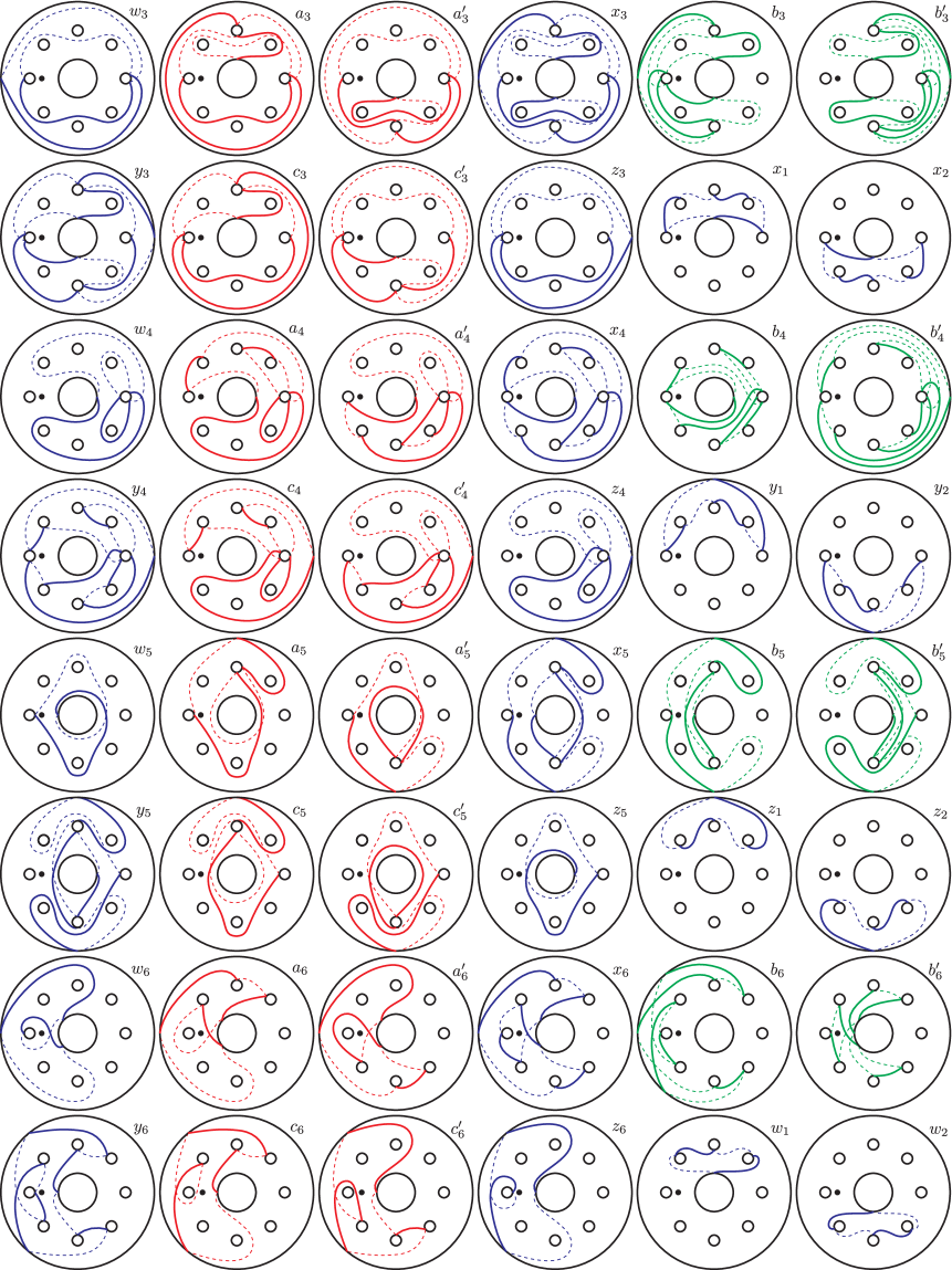
Refer to caption
Figure 23. Vanishing cycles of the genus–999 Lefschetz fibration with signature zero.

4. Proof of Theorem A

Here is an outline for our proof of Theorem A: Since the novel genus–999 Lefschetz fibration (X,f)𝑋𝑓(X,f) we built in the previous section will serve as one of the main building blocks of our constructions, we will first analyze the algebraic and differential topology of X𝑋X in some detail. We will then first prove all the statements for genus–999 fibrations, deferring the construction of higher genera examples till the end. We will first construct Lefschetz fibrations with prescribed signatures, and then the spin ones. All will be done by taking products of conjugated positive factorizations of the identity in Mod(Σg)ModsubscriptΣ𝑔\operatorname{Mod}(\Sigma_{g}) (corresponding to twisted fiber sums of the fibrations) and breedings (one of which corresponds to lantern substitution, thus the rational blowdown), which will require extra care in the spin case.

4.1. The topology of the signature zero genus-999 Lefschetz fibration

The essential information we need for later arguments is summed up as follows:

Theorem 14.

There is a symplectic genus–999 Lefschetz fibration (X,f)𝑋𝑓(X,f) with monodromy factorization

(18) t\scaletow39ptt\scaletoa39ptt\scaletoa39ptt\scaletox39ptt\scaletob39ptt\scaletob39ptt\scaletoy39ptt\scaletoc39ptt\scaletoc39ptt\scaletoz39ptt\scaletox19ptt\scaletox29ptt\scaletow49ptt\scaletoa49ptt\scaletoa49ptt\scaletox49ptt\scaletob49ptt\scaletob49ptt\scaletoy49ptt\scaletoc49ptt\scaletoc49ptt\scaletoz49ptt\scaletoy19ptt\scaletoy29ptsubscript𝑡\scaletosubscript𝑤39𝑝𝑡subscript𝑡\scaletosubscript𝑎39𝑝𝑡subscript𝑡\scaletosuperscriptsubscript𝑎39𝑝𝑡subscript𝑡\scaletosubscript𝑥39𝑝𝑡subscript𝑡\scaletosubscript𝑏39𝑝𝑡subscript𝑡\scaletosuperscriptsubscript𝑏39𝑝𝑡subscript𝑡\scaletosubscript𝑦39𝑝𝑡subscript𝑡\scaletosubscript𝑐39𝑝𝑡subscript𝑡\scaletosuperscriptsubscript𝑐39𝑝𝑡subscript𝑡\scaletosubscript𝑧39𝑝𝑡subscript𝑡\scaletosubscript𝑥19𝑝𝑡subscript𝑡\scaletosubscript𝑥29𝑝𝑡subscript𝑡\scaletosubscript𝑤49𝑝𝑡subscript𝑡\scaletosubscript𝑎49𝑝𝑡subscript𝑡\scaletosuperscriptsubscript𝑎49𝑝𝑡subscript𝑡\scaletosubscript𝑥49𝑝𝑡subscript𝑡\scaletosubscript𝑏49𝑝𝑡subscript𝑡\scaletosuperscriptsubscript𝑏49𝑝𝑡subscript𝑡\scaletosubscript𝑦49𝑝𝑡subscript𝑡\scaletosubscript𝑐49𝑝𝑡subscript𝑡\scaletosuperscriptsubscript𝑐49𝑝𝑡subscript𝑡\scaletosubscript𝑧49𝑝𝑡subscript𝑡\scaletosubscript𝑦19𝑝𝑡subscript𝑡\scaletosubscript𝑦29𝑝𝑡\displaystyle t_{\scaleto{\mathstrut w_{3}}{9pt}}t_{\scaleto{\mathstrut a_{3}}{9pt}}t_{\scaleto{\mathstrut a_{3}^{\prime}}{9pt}}t_{\scaleto{\mathstrut x_{3}}{9pt}}t_{\scaleto{\mathstrut b_{3}}{9pt}}t_{\scaleto{\mathstrut b_{3}^{\prime}}{9pt}}t_{\scaleto{\mathstrut y_{3}}{9pt}}t_{\scaleto{\mathstrut c_{3}}{9pt}}t_{\scaleto{\mathstrut c_{3}^{\prime}}{9pt}}t_{\scaleto{\mathstrut z_{3}}{9pt}}t_{\scaleto{\mathstrut x_{1}}{9pt}}t_{\scaleto{\mathstrut x_{2}}{9pt}}t_{\scaleto{\mathstrut w_{4}}{9pt}}t_{\scaleto{\mathstrut a_{4}}{9pt}}t_{\scaleto{\mathstrut a_{4}^{\prime}}{9pt}}t_{\scaleto{\mathstrut x_{4}}{9pt}}t_{\scaleto{\mathstrut b_{4}}{9pt}}t_{\scaleto{\mathstrut b_{4}^{\prime}}{9pt}}t_{\scaleto{\mathstrut y_{4}}{9pt}}t_{\scaleto{\mathstrut c_{4}}{9pt}}t_{\scaleto{\mathstrut c_{4}^{\prime}}{9pt}}t_{\scaleto{\mathstrut z_{4}}{9pt}}t_{\scaleto{\mathstrut y_{1}}{9pt}}t_{\scaleto{\mathstrut y_{2}}{9pt}}
t\scaletow59ptt\scaletoa59ptt\scaletoa59ptt\scaletox59ptt\scaletob59ptt\scaletob59ptt\scaletoy59ptt\scaletoc59ptt\scaletoc59ptt\scaletoz59ptt\scaletoz29ptt\scaletoz19ptt\scaletow69ptt\scaletoa69ptt\scaletoa69ptt\scaletox69ptt\scaletob69ptt\scaletob69ptt\scaletoy69ptt\scaletoc69ptt\scaletoc69ptt\scaletoz69ptt\scaletow19ptt\scaletow29pt=1,\displaystyle\cdot t_{\scaleto{\mathstrut w_{5}}{9pt}}t_{\scaleto{\mathstrut a_{5}}{9pt}}t_{\scaleto{\mathstrut a_{5}^{\prime}}{9pt}}t_{\scaleto{\mathstrut x_{5}}{9pt}}t_{\scaleto{\mathstrut b_{5}}{9pt}}t_{\scaleto{\mathstrut b_{5}^{\prime}}{9pt}}t_{\scaleto{\mathstrut y_{5}}{9pt}}t_{\scaleto{\mathstrut c_{5}}{9pt}}t_{\scaleto{\mathstrut c_{5}^{\prime}}{9pt}}t_{\scaleto{\mathstrut z_{5}}{9pt}}t_{\scaleto{\mathstrut z_{2}}{9pt}}t_{\scaleto{\mathstrut z_{1}}{9pt}}t_{\scaleto{\mathstrut w_{6}}{9pt}}t_{\scaleto{\mathstrut a_{6}}{9pt}}t_{\scaleto{\mathstrut a_{6}^{\prime}}{9pt}}t_{\scaleto{\mathstrut x_{6}}{9pt}}t_{\scaleto{\mathstrut b_{6}}{9pt}}t_{\scaleto{\mathstrut b_{6}^{\prime}}{9pt}}t_{\scaleto{\mathstrut y_{6}}{9pt}}t_{\scaleto{\mathstrut c_{6}}{9pt}}t_{\scaleto{\mathstrut c_{6}^{\prime}}{9pt}}t_{\scaleto{\mathstrut z_{6}}{9pt}}t_{\scaleto{\mathstrut w_{1}}{9pt}}t_{\scaleto{\mathstrut w_{2}}{9pt}}=1,

in Mod(Σ9)ModsubscriptΣ9\mathrm{Mod}(\Sigma_{9}), where the Dehn twist curves are as in Figure 23. The total space X𝑋X is a spin symplectic 444–manifold of general type, which is not deformation equivalent to any compact complex surface, where e(X)=16e𝑋16{\text{e}}(X)=16, σ(X)=0𝜎𝑋0\sigma(X)=0, and H1(X)=742subscript𝐻1𝑋direct-sumsuperscript7subscript4subscript2H_{1}(X)=\mathbb{Z}^{7}\oplus\mathbb{Z}_{4}\oplus\mathbb{Z}_{2}.

Proof.

The Lefschetz fibration (X,f)𝑋𝑓(X,f) prescribed by the positive factorization (18) we have constructed in the previous section, is a symplectic fibration with respect to a Gompf-Thurston symplectic form ω𝜔\omega we can equip it with. While it will take some effort to prove that X𝑋X is spin, all other claims on the differential topology of X𝑋X follow from our claims on its algebraic topology: For X𝑋X is spin, it is obviously minimal, and c12(X)=2e(X)+3σ(X)=32>0superscriptsubscript𝑐12𝑋2e𝑋3𝜎𝑋320c_{1}^{2}(X)=2{\text{e}}(X)+3\sigma(X)=32>0, so the Kodaira dimension of the symplectic 444–manifold (X,ω)𝑋𝜔(X,\omega) is κ(X)=2𝜅𝑋2\kappa(X)=2, in other words, it is of general type. Because b1(X)subscript𝑏1𝑋b_{1}(X) is odd, X𝑋X is not even homotopy equivalent to a compact complex surface of general type, which are all known to be Kähler.

We calculate the algebraic invariants of X𝑋X next.

Euler characteristic and signature: The Euler characteristic of X𝑋X is the easiest to calculate by the formula e(X)=44g+ne𝑋44𝑔𝑛{\text{e}}(X)=4-4g+n, where the genus of the Lefschetz fibration g=9𝑔9g=9, and the number of nodes, corresponding to the Dehn twists in the monodromy factorization, is n=48𝑛48n=48.

Although the calculation of the signature of a Lefschetz fibration usually requires computer assistance to run an algorithm, we leveraged the fact that we have built the monodromy factorization (18) for (X,f)𝑋𝑓(X,f) from scratch, using only basic relations in the mapping class group. Thanks to the work of Endo and Nagami [21], we easily calculate the signature of X𝑋X by an algebraic count of the relations we have employed to derive the final positive factorization of the identity in Mod(Σ9)ModsubscriptΣ9\operatorname{Mod}(\Sigma_{9}). Embeddings of relations into higher genera surfaces, cancellations of positive and negative Dehn twists, and Hurwitz moves do not affect the signature calculation. Since we built our genus–999 factorization through embeddings of the signature zero genus–333 relation, cancellations and Hurwitz moves, we conclude that σ(X)=0𝜎𝑋0\sigma(X)=0.

Note that we calculated the signature of our genus–222 and genus–333 pencils in the same way, recalling that every use of the 222–chain and the lantern relation contributes 77-7 and +11+1 to the signature count [21]. Algebraically, we used one 222–chain and seven lantern relations to derive the monodromy factorization of the genus–222 pencil, whereas these numbers are doubled for the genus–333 pencil. In turn, a total of 121212 222–chain and 848484 lantern relations yield the positive factorization for (X,f)𝑋𝑓(X,f). (These large numbers might demonstrate why it is more feasible to build such a relation in multiple steps via breedings.)

First homology: The total space of a genus–g𝑔g Lefschetz fibration over the 222–sphere has a handle decomposition (D2×Σg)ihi(D2×Σg)superscript𝐷2subscriptΣ𝑔subscript𝑖subscript𝑖superscript𝐷2subscriptΣ𝑔(D^{2}\times\Sigma_{g})\cup\,\sum_{i}h_{i}\,\cup(D^{2}\times\Sigma_{g}), where hisubscript𝑖h_{i} are 222–handles attached along the loops on ΣgsubscriptΣ𝑔\Sigma_{g}, which are the Dehn twist curves cisubscript𝑐𝑖c_{i} in the monodromy factorization of the fibration [31]. Therefore, the first homology of the total space can be calculated by taking a quotient H1(Σg)subscript𝐻1subscriptΣ𝑔H_{1}(\Sigma_{g}), as the first D2×Σgsuperscript𝐷2subscriptΣ𝑔D^{2}\times\Sigma_{g} contains all the 111–handles, by the abelianized relations induced by the attaching circles of all the 222–handles, which are the vanishing cycles cisubscript𝑐𝑖c_{i}, and the attaching circle of the last 222–handle coming from the second D2×Σgsuperscript𝐷2subscriptΣ𝑔D^{2}\times\Sigma_{g} in the above decomposition.

Accordingly, we will calculate H1(X)subscript𝐻1𝑋H_{1}(X) using the monodromy factorization of our genus–999 fibration. Let {αi,βi}subscript𝛼𝑖subscript𝛽𝑖\{\alpha_{i},\beta_{i}\} be the homology generators of H1(Σ9)subscript𝐻1subscriptΣ9H_{1}(\Sigma_{9}), represented by the loops in Figure 24. After picking an auxiliary orientation on each Dehn twist curve in Figure 23, and calculating the number of its algebraic intersections with {αi,βi}subscript𝛼𝑖subscript𝛽𝑖\{\alpha_{i},\beta_{i}\}, we can easily read off the relation induced by the corresponding vanishing cycle. We tabulate this data below in a way the coefficients are easily visible, as it will be vital to our arguments for determining the spin type of X𝑋X as well.

Refer to caption
Figure 24. The symplectic basis for H1(Σ9;)subscript𝐻1subscriptΣ9H_{1}(\Sigma_{9};\mathbb{Z}).

Homology classes of the vanishing cycles:

w3subscript𝑤3\displaystyle w_{3} =α1absentsubscript𝛼1\displaystyle=\alpha_{1} +2α22subscript𝛼2\displaystyle+2\alpha_{2} +2α32subscript𝛼3\displaystyle+2\alpha_{3} +2α42subscript𝛼4\displaystyle+2\alpha_{4} +α5subscript𝛼5\displaystyle+\alpha_{5} +2α62subscript𝛼6\displaystyle+2\alpha_{6} +2α72subscript𝛼7\displaystyle+2\alpha_{7} +2α82subscript𝛼8\displaystyle+2\alpha_{8} +2α92subscript𝛼9\displaystyle+2\alpha_{9} +2β32subscript𝛽3\displaystyle+2\beta_{3} β7subscript𝛽7\displaystyle-\beta_{7} ,
a3subscript𝑎3\displaystyle a_{3} =α1absentsubscript𝛼1\displaystyle=\alpha_{1} +3α23subscript𝛼2\displaystyle+3\alpha_{2} +2α32subscript𝛼3\displaystyle+2\alpha_{3} +2α42subscript𝛼4\displaystyle+2\alpha_{4} +α5subscript𝛼5\displaystyle+\alpha_{5} +2α62subscript𝛼6\displaystyle+2\alpha_{6} +2α72subscript𝛼7\displaystyle+2\alpha_{7} +3α83subscript𝛼8\displaystyle+3\alpha_{8} +2α92subscript𝛼9\displaystyle+2\alpha_{9} +2β32subscript𝛽3\displaystyle+2\beta_{3} β7subscript𝛽7\displaystyle-\beta_{7} β9,subscript𝛽9\displaystyle-\beta_{9},
a3superscriptsubscript𝑎3\displaystyle a_{3}^{\prime} =α1absentsubscript𝛼1\displaystyle=\alpha_{1} +2α22subscript𝛼2\displaystyle+2\alpha_{2} +2α32subscript𝛼3\displaystyle+2\alpha_{3} +3α43subscript𝛼4\displaystyle+3\alpha_{4} +α5subscript𝛼5\displaystyle+\alpha_{5} +3α63subscript𝛼6\displaystyle+3\alpha_{6} +2α72subscript𝛼7\displaystyle+2\alpha_{7} +2α82subscript𝛼8\displaystyle+2\alpha_{8} +2α92subscript𝛼9\displaystyle+2\alpha_{9} +2β32subscript𝛽3\displaystyle+2\beta_{3} β7subscript𝛽7\displaystyle-\beta_{7} β9,subscript𝛽9\displaystyle-\beta_{9},
x3subscript𝑥3\displaystyle x_{3} =α1absentsubscript𝛼1\displaystyle=\alpha_{1} +3α23subscript𝛼2\displaystyle+3\alpha_{2} +2α32subscript𝛼3\displaystyle+2\alpha_{3} +3α43subscript𝛼4\displaystyle+3\alpha_{4} +α5subscript𝛼5\displaystyle+\alpha_{5} +3α63subscript𝛼6\displaystyle+3\alpha_{6} +2α72subscript𝛼7\displaystyle+2\alpha_{7} +3α83subscript𝛼8\displaystyle+3\alpha_{8} +2α92subscript𝛼9\displaystyle+2\alpha_{9} +2β32subscript𝛽3\displaystyle+2\beta_{3} β7subscript𝛽7\displaystyle-\beta_{7} 2β9,2subscript𝛽9\displaystyle-2\beta_{9},
b3subscript𝑏3\displaystyle b_{3} =\displaystyle= α2subscript𝛼2\displaystyle\alpha_{2} +α4subscript𝛼4\displaystyle+\alpha_{4} +α6subscript𝛼6\displaystyle+\alpha_{6} +α8subscript𝛼8\displaystyle+\alpha_{8} +β7subscript𝛽7\displaystyle+\beta_{7} 2β9,2subscript𝛽9\displaystyle-2\beta_{9},
b3superscriptsubscript𝑏3\displaystyle b_{3}^{\prime} =\displaystyle= α2subscript𝛼2\displaystyle\alpha_{2} +α4subscript𝛼4\displaystyle+\alpha_{4} +α6subscript𝛼6\displaystyle+\alpha_{6} +α8subscript𝛼8\displaystyle+\alpha_{8} +β3subscript𝛽3\displaystyle+\beta_{3} 2β9,2subscript𝛽9\displaystyle-2\beta_{9},
y3subscript𝑦3\displaystyle y_{3} =α1absentsubscript𝛼1\displaystyle=\alpha_{1} +α2subscript𝛼2\displaystyle+\alpha_{2} +2α32subscript𝛼3\displaystyle+2\alpha_{3} +α4subscript𝛼4\displaystyle+\alpha_{4} +α5subscript𝛼5\displaystyle+\alpha_{5} +α6subscript𝛼6\displaystyle+\alpha_{6} +2α72subscript𝛼7\displaystyle+2\alpha_{7} +α8subscript𝛼8\displaystyle+\alpha_{8} +2α92subscript𝛼9\displaystyle+2\alpha_{9} +β3subscript𝛽3\displaystyle+\beta_{3} 2β72subscript𝛽7\displaystyle-2\beta_{7} +2β9,2subscript𝛽9\displaystyle+2\beta_{9},
c3subscript𝑐3\displaystyle c_{3} =α1absentsubscript𝛼1\displaystyle=\alpha_{1} +α2subscript𝛼2\displaystyle+\alpha_{2} +2α32subscript𝛼3\displaystyle+2\alpha_{3} +2α42subscript𝛼4\displaystyle+2\alpha_{4} +α5subscript𝛼5\displaystyle+\alpha_{5} +2α62subscript𝛼6\displaystyle+2\alpha_{6} +2α72subscript𝛼7\displaystyle+2\alpha_{7} +α8subscript𝛼8\displaystyle+\alpha_{8} +2α92subscript𝛼9\displaystyle+2\alpha_{9} +β3subscript𝛽3\displaystyle+\beta_{3} 2β72subscript𝛽7\displaystyle-2\beta_{7} +β9,subscript𝛽9\displaystyle+\beta_{9},
c3superscriptsubscript𝑐3\displaystyle c_{3}^{\prime} =α1absentsubscript𝛼1\displaystyle=\alpha_{1} +2α22subscript𝛼2\displaystyle+2\alpha_{2} +2α32subscript𝛼3\displaystyle+2\alpha_{3} +α4subscript𝛼4\displaystyle+\alpha_{4} +α5subscript𝛼5\displaystyle+\alpha_{5} +α6subscript𝛼6\displaystyle+\alpha_{6} +2α72subscript𝛼7\displaystyle+2\alpha_{7} +2α82subscript𝛼8\displaystyle+2\alpha_{8} +2α92subscript𝛼9\displaystyle+2\alpha_{9} +β3subscript𝛽3\displaystyle+\beta_{3} 2β72subscript𝛽7\displaystyle-2\beta_{7} +β9,subscript𝛽9\displaystyle+\beta_{9},
z3subscript𝑧3\displaystyle z_{3} =α1absentsubscript𝛼1\displaystyle=\alpha_{1} +2α22subscript𝛼2\displaystyle+2\alpha_{2} +2α32subscript𝛼3\displaystyle+2\alpha_{3} +2α42subscript𝛼4\displaystyle+2\alpha_{4} +α5subscript𝛼5\displaystyle+\alpha_{5} +2α62subscript𝛼6\displaystyle+2\alpha_{6} +2α72subscript𝛼7\displaystyle+2\alpha_{7} +2α82subscript𝛼8\displaystyle+2\alpha_{8} +2α92subscript𝛼9\displaystyle+2\alpha_{9} +β3subscript𝛽3\displaystyle+\beta_{3} 2β72subscript𝛽7\displaystyle-2\beta_{7} ,
x1subscript𝑥1\displaystyle x_{1} =\displaystyle= α2subscript𝛼2\displaystyle\alpha_{2} +α8subscript𝛼8\displaystyle+\alpha_{8} +β1subscript𝛽1\displaystyle+\beta_{1} β2subscript𝛽2\displaystyle-\beta_{2} +β3subscript𝛽3\displaystyle+\beta_{3} +β7subscript𝛽7\displaystyle+\beta_{7} β8subscript𝛽8\displaystyle-\beta_{8} β9,subscript𝛽9\displaystyle-\beta_{9},
x2subscript𝑥2\displaystyle x_{2} =\displaystyle= α4subscript𝛼4\displaystyle\alpha_{4} +α6subscript𝛼6\displaystyle+\alpha_{6} +β3subscript𝛽3\displaystyle+\beta_{3} β4subscript𝛽4\displaystyle-\beta_{4} +β5subscript𝛽5\displaystyle+\beta_{5} β6subscript𝛽6\displaystyle-\beta_{6} +β7subscript𝛽7\displaystyle+\beta_{7} β9,subscript𝛽9\displaystyle-\beta_{9},
w4subscript𝑤4\displaystyle w_{4} =α1absentsubscript𝛼1\displaystyle=\alpha_{1} +2α22subscript𝛼2\displaystyle+2\alpha_{2} +2α32subscript𝛼3\displaystyle+2\alpha_{3} +2α42subscript𝛼4\displaystyle+2\alpha_{4} +α5subscript𝛼5\displaystyle+\alpha_{5} +α6subscript𝛼6\displaystyle+\alpha_{6} +α8subscript𝛼8\displaystyle+\alpha_{8} +β3subscript𝛽3\displaystyle+\beta_{3} β9,subscript𝛽9\displaystyle-\beta_{9},
a4subscript𝑎4\displaystyle a_{4} =α1absentsubscript𝛼1\displaystyle=\alpha_{1} +2α22subscript𝛼2\displaystyle+2\alpha_{2} +2α32subscript𝛼3\displaystyle+2\alpha_{3} +2α42subscript𝛼4\displaystyle+2\alpha_{4} +α5subscript𝛼5\displaystyle+\alpha_{5} +α6subscript𝛼6\displaystyle+\alpha_{6} +α8subscript𝛼8\displaystyle+\alpha_{8} +β1subscript𝛽1\displaystyle+\beta_{1} β2subscript𝛽2\displaystyle-\beta_{2} +β3subscript𝛽3\displaystyle+\beta_{3} +β7subscript𝛽7\displaystyle+\beta_{7} β8subscript𝛽8\displaystyle-\beta_{8} β9,subscript𝛽9\displaystyle-\beta_{9},
a4superscriptsubscript𝑎4\displaystyle a_{4}^{\prime} =α1absentsubscript𝛼1\displaystyle=\alpha_{1} +2α22subscript𝛼2\displaystyle+2\alpha_{2} +2α32subscript𝛼3\displaystyle+2\alpha_{3} +2α42subscript𝛼4\displaystyle+2\alpha_{4} +α5subscript𝛼5\displaystyle+\alpha_{5} +α6subscript𝛼6\displaystyle+\alpha_{6} +α8subscript𝛼8\displaystyle+\alpha_{8} +β3subscript𝛽3\displaystyle+\beta_{3} β4subscript𝛽4\displaystyle-\beta_{4} +β5subscript𝛽5\displaystyle+\beta_{5} β6subscript𝛽6\displaystyle-\beta_{6} +β7subscript𝛽7\displaystyle+\beta_{7} β9,subscript𝛽9\displaystyle-\beta_{9},
x4subscript𝑥4\displaystyle x_{4} =α1absentsubscript𝛼1\displaystyle=\alpha_{1} +2α22subscript𝛼2\displaystyle+2\alpha_{2} +2α32subscript𝛼3\displaystyle+2\alpha_{3} +2α42subscript𝛼4\displaystyle+2\alpha_{4} +α5subscript𝛼5\displaystyle+\alpha_{5} +α6subscript𝛼6\displaystyle+\alpha_{6} +α8subscript𝛼8\displaystyle+\alpha_{8} +β1subscript𝛽1\displaystyle+\beta_{1} β2subscript𝛽2\displaystyle-\beta_{2} +β3subscript𝛽3\displaystyle+\beta_{3} β4subscript𝛽4\displaystyle-\beta_{4} +β5subscript𝛽5\displaystyle+\beta_{5} β6subscript𝛽6\displaystyle-\beta_{6} +2β72subscript𝛽7\displaystyle+2\beta_{7} β8subscript𝛽8\displaystyle-\beta_{8} β9,subscript𝛽9\displaystyle-\beta_{9},
b4subscript𝑏4\displaystyle b_{4} =\displaystyle= β1subscript𝛽1\displaystyle\beta_{1} β2subscript𝛽2\displaystyle-\beta_{2} +β3subscript𝛽3\displaystyle+\beta_{3} β4subscript𝛽4\displaystyle-\beta_{4} +β5subscript𝛽5\displaystyle+\beta_{5} β6subscript𝛽6\displaystyle-\beta_{6} +2β72subscript𝛽7\displaystyle+2\beta_{7} β8subscript𝛽8\displaystyle-\beta_{8} β9,subscript𝛽9\displaystyle-\beta_{9},
b4superscriptsubscript𝑏4\displaystyle b_{4}^{\prime} =\displaystyle= β1subscript𝛽1\displaystyle\beta_{1} β2subscript𝛽2\displaystyle-\beta_{2} +β3subscript𝛽3\displaystyle+\beta_{3} β4subscript𝛽4\displaystyle-\beta_{4} +β5subscript𝛽5\displaystyle+\beta_{5} β6subscript𝛽6\displaystyle-\beta_{6} +2β72subscript𝛽7\displaystyle+2\beta_{7} β8subscript𝛽8\displaystyle-\beta_{8} ,
y4subscript𝑦4\displaystyle y_{4} =α1absentsubscript𝛼1\displaystyle=\alpha_{1} +2α22subscript𝛼2\displaystyle+2\alpha_{2} +2α32subscript𝛼3\displaystyle+2\alpha_{3} +2α42subscript𝛼4\displaystyle+2\alpha_{4} +α5subscript𝛼5\displaystyle+\alpha_{5} +α6subscript𝛼6\displaystyle+\alpha_{6} +α8subscript𝛼8\displaystyle+\alpha_{8} β1subscript𝛽1\displaystyle-\beta_{1} +β2subscript𝛽2\displaystyle+\beta_{2} β3subscript𝛽3\displaystyle-\beta_{3} +β4subscript𝛽4\displaystyle+\beta_{4} β5subscript𝛽5\displaystyle-\beta_{5} +β6subscript𝛽6\displaystyle+\beta_{6} 2β72subscript𝛽7\displaystyle-2\beta_{7} +β8subscript𝛽8\displaystyle+\beta_{8} ,
c4subscript𝑐4\displaystyle c_{4} =α1absentsubscript𝛼1\displaystyle=\alpha_{1} +2α22subscript𝛼2\displaystyle+2\alpha_{2} +2α32subscript𝛼3\displaystyle+2\alpha_{3} +2α42subscript𝛼4\displaystyle+2\alpha_{4} +α5subscript𝛼5\displaystyle+\alpha_{5} +α6subscript𝛼6\displaystyle+\alpha_{6} +α8subscript𝛼8\displaystyle+\alpha_{8} β1subscript𝛽1\displaystyle-\beta_{1} +β2subscript𝛽2\displaystyle+\beta_{2} β3subscript𝛽3\displaystyle-\beta_{3} β7subscript𝛽7\displaystyle-\beta_{7} +β8subscript𝛽8\displaystyle+\beta_{8} ,
c4superscriptsubscript𝑐4\displaystyle c_{4}^{\prime} =α1absentsubscript𝛼1\displaystyle=\alpha_{1} +2α22subscript𝛼2\displaystyle+2\alpha_{2} +2α32subscript𝛼3\displaystyle+2\alpha_{3} +2α42subscript𝛼4\displaystyle+2\alpha_{4} +α5subscript𝛼5\displaystyle+\alpha_{5} +α6subscript𝛼6\displaystyle+\alpha_{6} +α8subscript𝛼8\displaystyle+\alpha_{8} β3subscript𝛽3\displaystyle-\beta_{3} +β4subscript𝛽4\displaystyle+\beta_{4} β5subscript𝛽5\displaystyle-\beta_{5} +β6subscript𝛽6\displaystyle+\beta_{6} β7subscript𝛽7\displaystyle-\beta_{7} ,
z4subscript𝑧4\displaystyle z_{4} =α1absentsubscript𝛼1\displaystyle=\alpha_{1} +2α22subscript𝛼2\displaystyle+2\alpha_{2} +2α32subscript𝛼3\displaystyle+2\alpha_{3} +2α42subscript𝛼4\displaystyle+2\alpha_{4} +α5subscript𝛼5\displaystyle+\alpha_{5} +α6subscript𝛼6\displaystyle+\alpha_{6} +α8subscript𝛼8\displaystyle+\alpha_{8} β3subscript𝛽3\displaystyle-\beta_{3} ,
y1subscript𝑦1\displaystyle y_{1} =\displaystyle= α2subscript𝛼2\displaystyle\alpha_{2} +α8subscript𝛼8\displaystyle+\alpha_{8} β1subscript𝛽1\displaystyle-\beta_{1} +β2subscript𝛽2\displaystyle+\beta_{2} β3subscript𝛽3\displaystyle-\beta_{3} β7subscript𝛽7\displaystyle-\beta_{7} +β8subscript𝛽8\displaystyle+\beta_{8} ,
y2subscript𝑦2\displaystyle y_{2} =\displaystyle= α4subscript𝛼4\displaystyle\alpha_{4} +α6subscript𝛼6\displaystyle+\alpha_{6} β3subscript𝛽3\displaystyle-\beta_{3} +β4subscript𝛽4\displaystyle+\beta_{4} β5subscript𝛽5\displaystyle-\beta_{5} +β6subscript𝛽6\displaystyle+\beta_{6} β7subscript𝛽7\displaystyle-\beta_{7} ,
w5subscript𝑤5\displaystyle w_{5} =α1absentsubscript𝛼1\displaystyle=\alpha_{1} +α5subscript𝛼5\displaystyle+\alpha_{5} +2α92subscript𝛼9\displaystyle+2\alpha_{9} β7subscript𝛽7\displaystyle-\beta_{7} +β9,subscript𝛽9\displaystyle+\beta_{9},
a5subscript𝑎5\displaystyle a_{5} =α1absentsubscript𝛼1\displaystyle=\alpha_{1} +α2subscript𝛼2\displaystyle+\alpha_{2} +α5subscript𝛼5\displaystyle+\alpha_{5} +α8subscript𝛼8\displaystyle+\alpha_{8} +2α92subscript𝛼9\displaystyle+2\alpha_{9} β7subscript𝛽7\displaystyle-\beta_{7} ,
a5superscriptsubscript𝑎5\displaystyle a_{5}^{\prime} =α1absentsubscript𝛼1\displaystyle=\alpha_{1} +α4subscript𝛼4\displaystyle+\alpha_{4} +α5subscript𝛼5\displaystyle+\alpha_{5} +α6subscript𝛼6\displaystyle+\alpha_{6} +2α92subscript𝛼9\displaystyle+2\alpha_{9} β7subscript𝛽7\displaystyle-\beta_{7} ,
x5subscript𝑥5\displaystyle x_{5} =α1absentsubscript𝛼1\displaystyle=\alpha_{1} +α2subscript𝛼2\displaystyle+\alpha_{2} +α4subscript𝛼4\displaystyle+\alpha_{4} +α5subscript𝛼5\displaystyle+\alpha_{5} +α6subscript𝛼6\displaystyle+\alpha_{6} +α8subscript𝛼8\displaystyle+\alpha_{8} +2α92subscript𝛼9\displaystyle+2\alpha_{9} β7subscript𝛽7\displaystyle-\beta_{7} β9,subscript𝛽9\displaystyle-\beta_{9},
b5subscript𝑏5\displaystyle b_{5} =\displaystyle= α2subscript𝛼2\displaystyle\alpha_{2} +α4subscript𝛼4\displaystyle+\alpha_{4} +α6subscript𝛼6\displaystyle+\alpha_{6} +α8subscript𝛼8\displaystyle+\alpha_{8} β7subscript𝛽7\displaystyle-\beta_{7} β9,subscript𝛽9\displaystyle-\beta_{9},
b5superscriptsubscript𝑏5\displaystyle b_{5}^{\prime} =\displaystyle= α2subscript𝛼2\displaystyle\alpha_{2} +α4subscript𝛼4\displaystyle+\alpha_{4} +α6subscript𝛼6\displaystyle+\alpha_{6} +α8subscript𝛼8\displaystyle+\alpha_{8} β3subscript𝛽3\displaystyle-\beta_{3} β9,subscript𝛽9\displaystyle-\beta_{9},
y5subscript𝑦5\displaystyle y_{5} =α1absentsubscript𝛼1\displaystyle=\alpha_{1} α2subscript𝛼2\displaystyle-\alpha_{2} α4subscript𝛼4\displaystyle-\alpha_{4} +α5subscript𝛼5\displaystyle+\alpha_{5} α6subscript𝛼6\displaystyle-\alpha_{6} α8subscript𝛼8\displaystyle-\alpha_{8} +2α92subscript𝛼9\displaystyle+2\alpha_{9} +β3subscript𝛽3\displaystyle+\beta_{3} +β9,subscript𝛽9\displaystyle+\beta_{9},
c5subscript𝑐5\displaystyle c_{5} =α1absentsubscript𝛼1\displaystyle=\alpha_{1} α2subscript𝛼2\displaystyle-\alpha_{2} +α5subscript𝛼5\displaystyle+\alpha_{5} α8subscript𝛼8\displaystyle-\alpha_{8} +2α92subscript𝛼9\displaystyle+2\alpha_{9} +β3subscript𝛽3\displaystyle+\beta_{3} ,
c5superscriptsubscript𝑐5\displaystyle c_{5}^{\prime} =α1absentsubscript𝛼1\displaystyle=\alpha_{1} α4subscript𝛼4\displaystyle-\alpha_{4} +α5subscript𝛼5\displaystyle+\alpha_{5} α6subscript𝛼6\displaystyle-\alpha_{6} +2α92subscript𝛼9\displaystyle+2\alpha_{9} +β3subscript𝛽3\displaystyle+\beta_{3} ,
z5subscript𝑧5\displaystyle z_{5} =α1absentsubscript𝛼1\displaystyle=\alpha_{1} +α5subscript𝛼5\displaystyle+\alpha_{5} +2α92subscript𝛼9\displaystyle+2\alpha_{9} +β3subscript𝛽3\displaystyle+\beta_{3} β9,subscript𝛽9\displaystyle-\beta_{9},
z1subscript𝑧1\displaystyle z_{1} =\displaystyle= α2subscript𝛼2\displaystyle\alpha_{2} +α8subscript𝛼8\displaystyle+\alpha_{8} +β1subscript𝛽1\displaystyle+\beta_{1} β2subscript𝛽2\displaystyle-\beta_{2} β8subscript𝛽8\displaystyle-\beta_{8} ,
z2subscript𝑧2\displaystyle z_{2} =\displaystyle= α4subscript𝛼4\displaystyle\alpha_{4} +α6subscript𝛼6\displaystyle+\alpha_{6} β4subscript𝛽4\displaystyle-\beta_{4} +β5subscript𝛽5\displaystyle+\beta_{5} β6subscript𝛽6\displaystyle-\beta_{6} ,
w6subscript𝑤6\displaystyle w_{6} =α1absentsubscript𝛼1\displaystyle=\alpha_{1} +α5subscript𝛼5\displaystyle+\alpha_{5} +α6subscript𝛼6\displaystyle+\alpha_{6} +2α72subscript𝛼7\displaystyle+2\alpha_{7} +α8subscript𝛼8\displaystyle+\alpha_{8} +β7subscript𝛽7\displaystyle+\beta_{7} 2β9,2subscript𝛽9\displaystyle-2\beta_{9},
a6subscript𝑎6\displaystyle a_{6} =α1absentsubscript𝛼1\displaystyle=\alpha_{1} +α5subscript𝛼5\displaystyle+\alpha_{5} +α6subscript𝛼6\displaystyle+\alpha_{6} +2α72subscript𝛼7\displaystyle+2\alpha_{7} +α8subscript𝛼8\displaystyle+\alpha_{8} β1subscript𝛽1\displaystyle-\beta_{1} +β2subscript𝛽2\displaystyle+\beta_{2} +β8subscript𝛽8\displaystyle+\beta_{8} 2β9,2subscript𝛽9\displaystyle-2\beta_{9},
a6superscriptsubscript𝑎6\displaystyle a_{6}^{\prime} =α1absentsubscript𝛼1\displaystyle=\alpha_{1} +α5subscript𝛼5\displaystyle+\alpha_{5} +α6subscript𝛼6\displaystyle+\alpha_{6} +2α72subscript𝛼7\displaystyle+2\alpha_{7} +α8subscript𝛼8\displaystyle+\alpha_{8} +β4subscript𝛽4\displaystyle+\beta_{4} β5subscript𝛽5\displaystyle-\beta_{5} +β6subscript𝛽6\displaystyle+\beta_{6} 2β9,2subscript𝛽9\displaystyle-2\beta_{9},
x6subscript𝑥6\displaystyle x_{6} =α1absentsubscript𝛼1\displaystyle=\alpha_{1} +α5subscript𝛼5\displaystyle+\alpha_{5} +α6subscript𝛼6\displaystyle+\alpha_{6} +2α72subscript𝛼7\displaystyle+2\alpha_{7} +α8subscript𝛼8\displaystyle+\alpha_{8} β1subscript𝛽1\displaystyle-\beta_{1} +β2subscript𝛽2\displaystyle+\beta_{2} +β4subscript𝛽4\displaystyle+\beta_{4} β5subscript𝛽5\displaystyle-\beta_{5} +β6subscript𝛽6\displaystyle+\beta_{6} β7subscript𝛽7\displaystyle-\beta_{7} +β8subscript𝛽8\displaystyle+\beta_{8} 2β9,2subscript𝛽9\displaystyle-2\beta_{9},
b6subscript𝑏6\displaystyle b_{6} =\displaystyle= β1subscript𝛽1\displaystyle\beta_{1} β2subscript𝛽2\displaystyle-\beta_{2} β4subscript𝛽4\displaystyle-\beta_{4} +β5subscript𝛽5\displaystyle+\beta_{5} β6subscript𝛽6\displaystyle-\beta_{6} +β7subscript𝛽7\displaystyle+\beta_{7} β8subscript𝛽8\displaystyle-\beta_{8} ,
b6superscriptsubscript𝑏6\displaystyle b_{6}^{\prime} =\displaystyle= β1subscript𝛽1\displaystyle\beta_{1} β2subscript𝛽2\displaystyle-\beta_{2} β4subscript𝛽4\displaystyle-\beta_{4} +β5subscript𝛽5\displaystyle+\beta_{5} β6subscript𝛽6\displaystyle-\beta_{6} +β7subscript𝛽7\displaystyle+\beta_{7} β8subscript𝛽8\displaystyle-\beta_{8} +β9,subscript𝛽9\displaystyle+\beta_{9},
y6subscript𝑦6\displaystyle y_{6} =α1absentsubscript𝛼1\displaystyle=\alpha_{1} +α5subscript𝛼5\displaystyle+\alpha_{5} +α6subscript𝛼6\displaystyle+\alpha_{6} +2α72subscript𝛼7\displaystyle+2\alpha_{7} +α8subscript𝛼8\displaystyle+\alpha_{8} +β1subscript𝛽1\displaystyle+\beta_{1} β2subscript𝛽2\displaystyle-\beta_{2} β4subscript𝛽4\displaystyle-\beta_{4} +β5subscript𝛽5\displaystyle+\beta_{5} β6subscript𝛽6\displaystyle-\beta_{6} +β7subscript𝛽7\displaystyle+\beta_{7} β8subscript𝛽8\displaystyle-\beta_{8} β9,subscript𝛽9\displaystyle-\beta_{9},
c6subscript𝑐6\displaystyle c_{6} =α1absentsubscript𝛼1\displaystyle=\alpha_{1} +α5subscript𝛼5\displaystyle+\alpha_{5} +α6subscript𝛼6\displaystyle+\alpha_{6} +2α72subscript𝛼7\displaystyle+2\alpha_{7} +α8subscript𝛼8\displaystyle+\alpha_{8} +β1subscript𝛽1\displaystyle+\beta_{1} β2subscript𝛽2\displaystyle-\beta_{2} β8subscript𝛽8\displaystyle-\beta_{8} β9,subscript𝛽9\displaystyle-\beta_{9},
c6superscriptsubscript𝑐6\displaystyle c_{6}^{\prime} =α1absentsubscript𝛼1\displaystyle=\alpha_{1} +α5subscript𝛼5\displaystyle+\alpha_{5} +α6subscript𝛼6\displaystyle+\alpha_{6} +2α72subscript𝛼7\displaystyle+2\alpha_{7} +α8subscript𝛼8\displaystyle+\alpha_{8} β4subscript𝛽4\displaystyle-\beta_{4} +β5subscript𝛽5\displaystyle+\beta_{5} β6subscript𝛽6\displaystyle-\beta_{6} β9,subscript𝛽9\displaystyle-\beta_{9},
z6subscript𝑧6\displaystyle z_{6} =α1absentsubscript𝛼1\displaystyle=\alpha_{1} +α5subscript𝛼5\displaystyle+\alpha_{5} +α6subscript𝛼6\displaystyle+\alpha_{6} +2α72subscript𝛼7\displaystyle+2\alpha_{7} +α8subscript𝛼8\displaystyle+\alpha_{8} β7subscript𝛽7\displaystyle-\beta_{7} β9,subscript𝛽9\displaystyle-\beta_{9},
w1subscript𝑤1\displaystyle w_{1} =\displaystyle= α2subscript𝛼2\displaystyle\alpha_{2} +α8subscript𝛼8\displaystyle+\alpha_{8} β1subscript𝛽1\displaystyle-\beta_{1} +β2subscript𝛽2\displaystyle+\beta_{2} +β8subscript𝛽8\displaystyle+\beta_{8} β9,subscript𝛽9\displaystyle-\beta_{9},
w2subscript𝑤2\displaystyle w_{2} =\displaystyle= α4subscript𝛼4\displaystyle\alpha_{4} +α6subscript𝛼6\displaystyle+\alpha_{6} +β4subscript𝛽4\displaystyle+\beta_{4} β5subscript𝛽5\displaystyle-\beta_{5} +β6subscript𝛽6\displaystyle+\beta_{6} β9.subscript𝛽9\displaystyle-\beta_{9}.

Recall that there is one more 222–handle we have to consider, and as we explained in the proof of Proposition 8 in Section 2, its attaching circle is homologous to the sum of the oriented curves of the point-pushing maps for any chosen marked point inducing a lift of the monodromy factorization from Mod(Σ9)ModsubscriptΣ9\operatorname{Mod}(\Sigma_{9}) to Mod(Σ9,1)ModsubscriptΣ91\operatorname{Mod}(\Sigma_{9,1}). (If we could find a section of (X,f)𝑋𝑓(X,f), the lift for the corresponding marked point would have no point-pushing maps, so this homology class would be trivial.) Looking at the point-pushing map in the relation (17) in Mod(Σ9,1)ModsubscriptΣ91\operatorname{Mod}(\Sigma_{9,1}) we get the following additional relation in homology:

s=α2+α8+β4β5+β6β7β9=0𝑠subscript𝛼2subscript𝛼8subscript𝛽4subscript𝛽5subscript𝛽6subscript𝛽7subscript𝛽90s=\alpha_{2}+\alpha_{8}+\beta_{4}-\beta_{5}+\beta_{6}-\beta_{7}-\beta_{9}=0\,

With this explicit presentation in hand, determining the finitely generated abelian group H1(X)subscript𝐻1𝑋H_{1}(X) is now a straightforward calculation. We will show that H1(X)=742.subscript𝐻1𝑋direct-sumsuperscript7subscript4subscript2H_{1}(X)=\mathbb{Z}^{7}\oplus\mathbb{Z}_{4}\oplus\mathbb{Z}_{2}.

From b4b4=β9superscriptsubscript𝑏4subscript𝑏4subscript𝛽9b_{4}^{\prime}-b_{4}=\beta_{9} we see β9=0subscript𝛽90\beta_{9}=0. Then, a3w3=α2+α8β9subscript𝑎3subscript𝑤3subscript𝛼2subscript𝛼8subscript𝛽9a_{3}-w_{3}=\alpha_{2}+\alpha_{8}-\beta_{9}, a3w3=α4+α6β9superscriptsubscript𝑎3subscript𝑤3subscript𝛼4subscript𝛼6subscript𝛽9a_{3}^{\prime}-w_{3}=\alpha_{4}+\alpha_{6}-\beta_{9} give α2+α8=0subscript𝛼2subscript𝛼80\alpha_{2}+\alpha_{8}=0, α4+α6=0subscript𝛼4subscript𝛼60\alpha_{4}+\alpha_{6}=0. Since b3=β7subscript𝑏3subscript𝛽7b_{3}=\beta_{7} modulo β9=α2+α8=α4+α6=0subscript𝛽9subscript𝛼2subscript𝛼8subscript𝛼4subscript𝛼60\beta_{9}=\alpha_{2}+\alpha_{8}=\alpha_{4}+\alpha_{6}=0, we have β7=0subscript𝛽70\beta_{7}=0. Similarly, b3=0superscriptsubscript𝑏30b_{3}^{\prime}=0 gives β3=0subscript𝛽30\beta_{3}=0. Now x1=β1β2β8subscript𝑥1subscript𝛽1subscript𝛽2subscript𝛽8x_{1}=\beta_{1}-\beta_{2}-\beta_{8} and x2=β4+β5β6subscript𝑥2subscript𝛽4subscript𝛽5subscript𝛽6x_{2}=-\beta_{4}+\beta_{5}-\beta_{6} modulo β9=α2+α8=α4+α6=β3=β7=0subscript𝛽9subscript𝛼2subscript𝛼8subscript𝛼4subscript𝛼6subscript𝛽3subscript𝛽70\beta_{9}=\alpha_{2}+\alpha_{8}=\alpha_{4}+\alpha_{6}=\beta_{3}=\beta_{7}=0, thus β1β2β8=β4+β5β6=0subscript𝛽1subscript𝛽2subscript𝛽8subscript𝛽4subscript𝛽5subscript𝛽60\beta_{1}-\beta_{2}-\beta_{8}=-\beta_{4}+\beta_{5}-\beta_{6}=0, or β1=β2+β8subscript𝛽1subscript𝛽2subscript𝛽8\beta_{1}=\beta_{2}+\beta_{8} and β5=β4+β6subscript𝛽5subscript𝛽4subscript𝛽6\beta_{5}=\beta_{4}+\beta_{6}. From w5=0subscript𝑤50w_{5}=0 with β7=β9=0subscript𝛽7subscript𝛽90\beta_{7}=\beta_{9}=0 we see α1+α5+2α9=0subscript𝛼1subscript𝛼52subscript𝛼90\alpha_{1}+\alpha_{5}+2\alpha_{9}=0. Looking at w3=0subscript𝑤30w_{3}=0 together with α1+α5+2α9=α2+α8=α4+α6=β3=β7=0subscript𝛼1subscript𝛼52subscript𝛼9subscript𝛼2subscript𝛼8subscript𝛼4subscript𝛼6subscript𝛽3subscript𝛽70\alpha_{1}+\alpha_{5}+2\alpha_{9}=\alpha_{2}+\alpha_{8}=\alpha_{4}+\alpha_{6}=\beta_{3}=\beta_{7}=0 we get 2α3+2α7=02subscript𝛼32subscript𝛼702\alpha_{3}+2\alpha_{7}=0. Combining 0=w4+w6=2α1+2α2+2α3+2α4+2α5+2α6+2α7+2α8+β3+β73β90subscript𝑤4subscript𝑤62subscript𝛼12subscript𝛼22subscript𝛼32subscript𝛼42subscript𝛼52subscript𝛼62subscript𝛼72subscript𝛼8subscript𝛽3subscript𝛽73subscript𝛽90=w_{4}+w_{6}=2\alpha_{1}+2\alpha_{2}+2\alpha_{3}+2\alpha_{4}+2\alpha_{5}+2\alpha_{6}+2\alpha_{7}+2\alpha_{8}+\beta_{3}+\beta_{7}-3\beta_{9} and α2+α8=α4+α6=2α3+2α7=β3=β7=β9=0subscript𝛼2subscript𝛼8subscript𝛼4subscript𝛼62subscript𝛼32subscript𝛼7subscript𝛽3subscript𝛽7subscript𝛽90\alpha_{2}+\alpha_{8}=\alpha_{4}+\alpha_{6}=2\alpha_{3}+2\alpha_{7}=\beta_{3}=\beta_{7}=\beta_{9}=0 we obtain 2α1+2α5=02subscript𝛼12subscript𝛼502\alpha_{1}+2\alpha_{5}=0. Since we also know α1+α5+2α9=0subscript𝛼1subscript𝛼52subscript𝛼90\alpha_{1}+\alpha_{5}+2\alpha_{9}=0 we deduce 4α9=04subscript𝛼904\alpha_{9}=0. We turn to w6=0subscript𝑤60w_{6}=0 and substitute α1+α5=2α9,β7=β9=0formulae-sequencesubscript𝛼1subscript𝛼52subscript𝛼9subscript𝛽7subscript𝛽90\alpha_{1}+\alpha_{5}=2\alpha_{9},\beta_{7}=\beta_{9}=0 to get 2α9+α6+2α7+α8=02subscript𝛼9subscript𝛼62subscript𝛼7subscript𝛼80-2\alpha_{9}+\alpha_{6}+2\alpha_{7}+\alpha_{8}=0, or α8=α62α7+2α9subscript𝛼8subscript𝛼62subscript𝛼72subscript𝛼9\alpha_{8}=-\alpha_{6}-2\alpha_{7}+2\alpha_{9}. In summary, we have

2(α3+α7)=0;2subscript𝛼3subscript𝛼70\displaystyle 2(\alpha_{3}+\alpha_{7})=0;
4α9=0;4subscript𝛼90\displaystyle 4\alpha_{9}=0;
α2=α8=α6+2α72α9;subscript𝛼2subscript𝛼8subscript𝛼62subscript𝛼72subscript𝛼9\displaystyle\alpha_{2}=-\alpha_{8}=\alpha_{6}+2\alpha_{7}-2\alpha_{9};
α4=α6;subscript𝛼4subscript𝛼6\displaystyle\alpha_{4}=-\alpha_{6};
α5=α12α9;subscript𝛼5subscript𝛼12subscript𝛼9\displaystyle\alpha_{5}=-\alpha_{1}-2\alpha_{9};
α8=α62α7+2α9;subscript𝛼8subscript𝛼62subscript𝛼72subscript𝛼9\displaystyle\alpha_{8}=-\alpha_{6}-2\alpha_{7}+2\alpha_{9};
β1=β2+β8;subscript𝛽1subscript𝛽2subscript𝛽8\displaystyle\beta_{1}=\beta_{2}+\beta_{8};
β3=0;subscript𝛽30\displaystyle\beta_{3}=0;
β5=β4+β6;subscript𝛽5subscript𝛽4subscript𝛽6\displaystyle\beta_{5}=\beta_{4}+\beta_{6};
β7=0;subscript𝛽70\displaystyle\beta_{7}=0;
β9=0.subscript𝛽90\displaystyle\beta_{9}=0.

It is easy to check that any other relations that come from the vanishing cycles can be deduced from the above relations. The extra relation coming from the point-pushing map is

s=α2+α8+β4β5+β6β7β9=0𝑠subscript𝛼2subscript𝛼8subscript𝛽4subscript𝛽5subscript𝛽6subscript𝛽7subscript𝛽90s=\alpha_{2}+\alpha_{8}+\beta_{4}-\beta_{5}+\beta_{6}-\beta_{7}-\beta_{9}=0

However, this relation can be deduced already from the relations coming from vanishing cycles since α2+α8=β4β5+β6=β7=β9=0subscript𝛼2subscript𝛼8subscript𝛽4subscript𝛽5subscript𝛽6subscript𝛽7subscript𝛽90\alpha_{2}+\alpha_{8}=\beta_{4}-\beta_{5}+\beta_{6}=\beta_{7}=\beta_{9}=0. This implies that we have a pseudosection. So we can take g1=α1,g2=α3,g3=α6,g4=β2,g5=β4,g6=β6,g7=β8,g8=α9,g9=α3+α7formulae-sequencesubscript𝑔1subscript𝛼1formulae-sequencesubscript𝑔2subscript𝛼3formulae-sequencesubscript𝑔3subscript𝛼6formulae-sequencesubscript𝑔4subscript𝛽2formulae-sequencesubscript𝑔5subscript𝛽4formulae-sequencesubscript𝑔6subscript𝛽6formulae-sequencesubscript𝑔7subscript𝛽8formulae-sequencesubscript𝑔8subscript𝛼9subscript𝑔9subscript𝛼3subscript𝛼7g_{1}=\alpha_{1},g_{2}=\alpha_{3},g_{3}=\alpha_{6},g_{4}=\beta_{2},g_{5}=\beta_{4},g_{6}=\beta_{6},g_{7}=\beta_{8},g_{8}=\alpha_{9},g_{9}=\alpha_{3}+\alpha_{7} as generators and the only relations among them are 4g8=04subscript𝑔804g_{8}=0 and 2g9=02subscript𝑔902g_{9}=0. We conclude that

H1(X)=742.subscript𝐻1𝑋direct-sumsuperscript7subscript4subscript2H_{1}(X)=\mathbb{Z}^{7}\oplus\mathbb{Z}_{4}\oplus\mathbb{Z}_{2}.

Other algebraic invariants: While we can derive an explicit presentation of π1(X)subscript𝜋1𝑋\pi_{1}(X) in the same fashion we did for H1(X)subscript𝐻1𝑋H_{1}(X) earlier, we will not actually need all of this more massive presentation for any of our arguments to follow, even the ones that involve killing the fundamental group. Instead, it will suffice to observe that in the monodromy factorization of (X,f)𝑋𝑓(X,f), we have three disjoint nonseparating curves, coming from the bounding quadruple of curves x1,z1,x2,z2subscript𝑥1subscript𝑧1subscript𝑥2subscript𝑧2x_{1},z_{1},x_{2},z_{2}; see Figure 25. These three curves simultaneously kill three generators of π1(Σ9)subscript𝜋1subscriptΣ9\pi_{1}(\Sigma_{9}).

Refer to caption
Figure 25. The bounding quadruple.

As it is the case for any closed oriented 444–manifold, the remaining homology groups of X𝑋X, as well as b2+(X)superscriptsubscript𝑏2𝑋b_{2}^{+}(X) and b2(X)superscriptsubscript𝑏2𝑋b_{2}^{-}(X), are already determined by e(X)e𝑋{\text{e}}(X), σ(X)𝜎𝑋\sigma(X) and H1(X)subscript𝐻1𝑋H_{1}(X) by Poincaré duality and the universal coefficient theorem. In particular, H2(X)=2842subscript𝐻2𝑋direct-sumsuperscript28subscript4subscript2H_{2}(X)=\mathbb{Z}^{28}\oplus\mathbb{Z}_{4}\oplus\mathbb{Z}_{2} and b2+(X)=b2(X)=14superscriptsubscript𝑏2𝑋superscriptsubscript𝑏2𝑋14b_{2}^{+}(X)=b_{2}^{-}(X)=14. Moreover X𝑋X can be seen to have an even intersection form, which will follow from its spin type.

Spin type: To build a spin Lefschetz fibration, our heuristic has been to breed exclusively Lefschetz pencils on spin 444–manifolds, as the monodromy factorizations of such pencils consist of Dehn twists that preserve a spin structure on a compact surface with boundary [14]. The groundwork for describing spin structures on X𝑋X was laid out in Section 2, and particularly in Theorem 9.

From our calculation of the \mathbb{Z}–homology classes of the vanishing cycles on Σ9subscriptΣ9\Sigma_{9} in the symplectic basis {αi,βi}subscript𝛼𝑖subscript𝛽𝑖\{\alpha_{i},\beta_{i}\} represented by the oriented curves with the same labels in Figure 24, we easily deduce the 2subscript2\mathbb{Z}_{2}–homology classes of them. We will single out two spin structures on X𝑋X, restrictions of which to the regular fiber will have different Arf invariants. Let the quadratic form q0subscript𝑞0q_{0} on H1(Σ9;2)subscript𝐻1subscriptΣ9subscript2H_{1}(\Sigma_{9};\mathbb{Z}_{2}) be defined by

q0(αi)=q0(βj)=1 for all i,j except for q0(β9)=0,subscript𝑞0subscript𝛼𝑖subscript𝑞0subscript𝛽𝑗1 for all i,j except for subscript𝑞0subscript𝛽90q_{0}(\alpha_{i})=q_{0}(\beta_{j})=1\text{ for all $i,j$ except for }q_{0}(\beta_{9})=0\,,

and the quadratic form q1subscript𝑞1q_{1} by

q1(αi)=q1(βj)=1 for all i,j except for q1(α7)=q1(β9)=0.subscript𝑞1subscript𝛼𝑖subscript𝑞1subscript𝛽𝑗1 for all i,j except for subscript𝑞1subscript𝛼7subscript𝑞1subscript𝛽90q_{1}(\alpha_{i})=q_{1}(\beta_{j})=1\text{ for all $i,j$ except for }q_{1}(\alpha_{7})=q_{1}(\beta_{9})=0\,.

Both are easily seen to evaluate as 111 on all the vanishing cycles. Let s0,s1Spin(Σg)subscript𝑠0subscript𝑠1SpinsubscriptΣ𝑔s_{0},s_{1}\in\mathrm{Spin}(\Sigma_{g}) be the spin structures corresponding to these two forms q0,q1subscript𝑞0subscript𝑞1q_{0},q_{1}, which have Arf invariants Arf(q0)=0Arfsubscript𝑞00\mathrm{Arf}(q_{0})=0 and Arf(q1)=1Arfsubscript𝑞11\mathrm{Arf}(q_{1})=1, respectively.

Next, recall that the homology relation α2+α8+β4β5+β6β7β9=0subscript𝛼2subscript𝛼8subscript𝛽4subscript𝛽5subscript𝛽6subscript𝛽7subscript𝛽90\alpha_{2}+\alpha_{8}+\beta_{4}-\beta_{5}+\beta_{6}-\beta_{7}-\beta_{9}=0 induced by the pseudosection s𝑠s is already generated by the relations induced by the vanishing cycles we listed during our calculation of H1(X)subscript𝐻1𝑋H_{1}(X). So by Proposition 8, the homology class of the regular fiber [F]delimited-[]𝐹[F] is primitive in H2(X)subscript𝐻2𝑋H_{2}(X). As we have (X,f)𝑋𝑓(X,f) with a primitive fiber class and signature σ(X)0𝜎𝑋0\sigma(X)\equiv 0 (mod 161616), by Theorem 9, the existence of the quadratic form q1subscript𝑞1q_{1} with Arf(q1)=1Arfsubscript𝑞11\textrm{Arf}(q_{1})=1 now implies that we have spin structures 𝔰isubscript𝔰𝑖\mathfrak{s}_{i} on X𝑋X coming from the spin structures sisubscript𝑠𝑖s_{i}, for each i=0,1𝑖01i=0,1. Note that 𝔰0,𝔰1subscript𝔰0subscript𝔰1\mathfrak{s}_{0},\mathfrak{s}_{1} are only two of the 512 spin structures on X𝑋X, for H1(X;2)=29superscript𝐻1𝑋subscript2superscriptsubscript29H^{1}(X;\mathbb{Z}_{2})=\mathbb{Z}_{2}^{9} acts freely and transitively on Spin(X)Spin𝑋\textrm{Spin}(X). ∎

Remark 15.

It might be interesting for symplectic construction enthusiasts to observe how the topology of the pieces we built evolved: Our most elementary building blocks are a genus–00 pencil (corresponding to the lantern relation) and genus–111 pencils (corresponding to 666–holed torus and 222–chain relations) on rational surfaces, breeding of which gives us a genus–222 pencil on the ruled surface T2×S2superscript𝑇2superscript𝑆2T^{2}\times S^{2}. All have symplectic Kodaira dimension κ=𝜅\kappa=-\infty. Using copies of the genus–222 pencil on the ruled surface, we obtained a symplectic Calabi-Yau 444–torus, which has κ=0𝜅0\kappa=0. We can also re-present our construction of the genus–999 fibration so that it is made out of two copies of a genus–555 pencil (each one of which is obtained by breeding a pair of our genus–333 pencils), along with two more copies of the genus–333 pencil. These genus–555 pencils have κ=1𝜅1\kappa=1. Lastly, our resulting genus–999 fibration (X,f)𝑋𝑓(X,f) yields a symplectic 444–manifold with κ=2𝜅2\kappa=2.

Remark 16.

Although we have used the breeding technique to effectively produce symplectic 444–manifolds out of smaller symplectic 444–manifolds, it is not inherently a symplectic operation. One first produces achiral pencils/fibrations on 444–manifolds that are often not symplectic, and only after pairing the vanishing cycles of all the negative nodes with matching vanishing cycles for positive nodes we can eliminate them to get a symplectic pencil/fibration. In general, the matching pairs would be visible only after a sequence of Hurwitz moves, or equivalently, a sequence of handle slides between the Lefschetz 222–handles. To approximate a surgery description, one can interpret the breeding construction as a two step process, where one first takes a fiber sum of achiral fibrations, whose monodromies are now supported on a larger surface, and then attaches a 555–dimensional 333–handle. (The latter can be seen by looking at the handle diagram of the neighborhood of the two matching nodes; see [12].) As observed in [31], when this matching vanishing cycle is trivial in the fundamental group of the complement, eliminating the two Lefschetz 222–handles is equivalent to removing an S2×S2superscript𝑆2superscript𝑆2S^{2}\times S^{2} or S2×S2superscript𝑆2superscript𝑆2S^{2}\mathbin{\mathchoice{\ooalign{\raise 4.95134pt\hbox{$\scriptstyle\sim$}\cr$\times$\cr}}{\ooalign{\raise 4.95134pt\hbox{$\scriptstyle\sim$}\cr$\times$\cr}}{\ooalign{\raise 3.65973pt\hbox{$\scriptscriptstyle\sim$}\cr$\scriptstyle\times$\cr}}{\ooalign{\raise 2.79857pt\hbox{$\scriptscriptstyle\sim$}\cr$\scriptscriptstyle\times$\cr}}}S^{2} summand from a connected sum (and capping off with D4superscript𝐷4D^{4}).

4.2. Lefschetz fibrations with prescribed signatures

We are now ready to prove our main theorem.

Proof of Theorem A.  To keep our presentation simple, here we will not attempt to keep the topology of the arbitrary signature examples small, but instead, we will refine our arguments in specific cases, as we will do so in Section 5. In fact, the following bit of information will be enough to run all our arguments: There is a signature zero genus–999 Lefschetz fibration (X,f)𝑋𝑓(X,f), where X𝑋X is spin and π1(X)subscript𝜋1𝑋\pi_{1}(X) has subgroups of arbitrarily large index. The existence of such a fibration is guaranteed by Theorem 14. We can assume, after a global conjugation, that the Lefschetz fibration (X,f)𝑋𝑓(X,f) has a monodromy factorization in Mod(Σ9)ModsubscriptΣ9\operatorname{Mod}(\Sigma_{9}):

(19) tB1P1=1,subscript𝑡subscript𝐵1subscript𝑃11t_{B_{1}}\,P_{1}=1\,,

where P1subscript𝑃1P_{1} is a product of positive Dehn twists, and B1subscript𝐵1B_{1} is the non-separating curve in Figure 26(a).

Any signature:  There are ϕ1,ϕ2Mod(Σ9)subscriptitalic-ϕ1subscriptitalic-ϕ2ModsubscriptΣ9\phi_{1},\phi_{2}\in\operatorname{Mod}(\Sigma_{9}) such that ϕ1(B1)=B2subscriptitalic-ϕ1subscript𝐵1subscript𝐵2\phi_{1}(B_{1})=B_{2} and ϕ2(B1)=B2subscriptitalic-ϕ2subscript𝐵1subscriptsuperscript𝐵2\phi_{2}(B_{1})=B^{\prime}_{2}, where B1,B2subscript𝐵1subscript𝐵2B_{1},B_{2} and B2subscriptsuperscript𝐵2B^{\prime}_{2} are the curves shown in Figure 26(a). Conjugating the monodromy factorization (19) with ϕisubscriptitalic-ϕ𝑖\phi_{i} for each i=1,2𝑖12i=1,2, we get  tB2P2=1subscript𝑡subscript𝐵2subscript𝑃21t_{B_{2}}P_{2}=1 and tB2P3=1subscript𝑡subscriptsuperscript𝐵2subscript𝑃31t_{B^{\prime}_{2}}P_{3}=1 in Mod(Σ9)ModsubscriptΣ9\operatorname{Mod}(\Sigma_{9}), where Pi=P1ϕisubscript𝑃𝑖superscriptsubscript𝑃1subscriptitalic-ϕ𝑖P_{i}=P_{1}^{\phi_{i}} is the product of positive Dehn twists along the images of the Dehn twist curves in P1subscript𝑃1P_{1} under ϕisubscriptitalic-ϕ𝑖\phi_{i}, in the same word order. After cyclic permutations, we get product factorizations  tB1P1P1tB1=1subscript𝑡subscript𝐵1subscript𝑃1subscript𝑃1subscript𝑡subscript𝐵11t_{B_{1}}P_{1}\cdot P_{1}t_{B_{1}}=1 and  tB2P2P3tB2=1subscript𝑡subscript𝐵2subscript𝑃2subscript𝑃3subscript𝑡subscriptsuperscript𝐵21t_{B_{2}}P_{2}\cdot P_{3}t_{B^{\prime}_{2}}=1, and in turn, we get

(20) tB12tB2tB2P12P2P3=1superscriptsubscript𝑡subscript𝐵12subscript𝑡subscript𝐵2subscript𝑡subscriptsuperscript𝐵2superscriptsubscript𝑃12subscript𝑃2subscript𝑃31t_{B_{1}}^{2}t_{B_{2}}t_{B^{\prime}_{2}}P_{1}^{2}P_{2}P_{3}=1

in Mod(Σ9)ModsubscriptΣ9\operatorname{Mod}(\Sigma_{9}), where tB1,tB2subscript𝑡subscript𝐵1subscript𝑡subscript𝐵2t_{B_{1}},t_{B_{2}} and tB2subscript𝑡subscriptsuperscript𝐵2t_{B^{\prime}_{2}} all commute with each other. The signature of the corresponding Lefschetz fibration, which is nothing but a twisted fiber sum of four copies of the signature zero fibration (X,f)𝑋𝑓(X,f), is zero. Since B1subscript𝐵1B_{1}, B1subscriptsuperscript𝐵1B^{\prime}_{1}, B2subscript𝐵2B_{2} and B2subscriptsuperscript𝐵2B^{\prime}_{2} (where B1subscriptsuperscript𝐵1B^{\prime}_{1} is isotopic to B1subscript𝐵1B_{1}) cobound a subsurface Σ04superscriptsubscriptΣ04\Sigma_{0}^{4}, we can make a lantern substitution (or equivalently breed with the genus–00 pencil on 2{\mathbb{CP}}{}^{2}) in the monodromy factorization (20), and get

(21) tXtYtZP12P2P3=1subscript𝑡𝑋subscript𝑡𝑌subscript𝑡𝑍superscriptsubscript𝑃12subscript𝑃2subscript𝑃31t_{X}t_{Y}t_{Z}P_{1}^{2}P_{2}P_{3}=1\,

in Mod(Σ9)ModsubscriptΣ9\operatorname{Mod}(\Sigma_{9}), where X,Y,Z𝑋𝑌𝑍X,Y,Z are the images of the standard lantern curves under the embedding of the above Σ22superscriptsubscriptΣ22\Sigma_{2}^{2} into Σ9subscriptΣ9\Sigma_{9}. Since the signature of the lantern relation is 111, the factorization (21) prescribes a new Lefschetz fibration (X1,f1)subscript𝑋1subscript𝑓1(X_{1},f_{1}) with σ(X1)=1𝜎subscript𝑋11\sigma(X_{1})=1.

Refer to caption
(a)
Refer to caption
(b)
Figure 26. Embeddings of lantern and 555–chain relation curves.

By taking fiber sum of copies of (X1,f1)subscript𝑋1subscript𝑓1(X_{1},f_{1}) with copies of any genus–999 Lefschetz fibration with a negative signature, we get Lefschetz fibrations (Xk,fk)subscript𝑋𝑘subscript𝑓𝑘(X_{k},f_{k}) with σ(Xk)=k𝜎subscript𝑋𝑘𝑘\sigma(X_{k})=k, for any prescribed k𝑘k\in\mathbb{Z}. For instance, by taking fiber sum of k𝑘k copies of (X1,f1)subscript𝑋1subscript𝑓1(X_{1},f_{1}), we obtain a Lefschetz fibration (Xk,fk)subscript𝑋𝑘subscript𝑓𝑘(X_{k},f_{k}) with σ(Xk)=k𝜎subscript𝑋𝑘𝑘\sigma(X_{k})=k, for any k+𝑘superscriptk\in\mathbb{Z}^{+}. If we employ in this procedure any of the Lefschetz fibrations discussed in Example 6, since their vanishing cycles already kill π1(Σg)subscript𝜋1subscriptΣ𝑔\pi_{1}(\Sigma_{g}), we get simply-connected examples, with prescribed signature. For example, we can take the fiber sum of (X41,f41)subscript𝑋41subscript𝑓41(X_{41},f_{41}) with a genus–999 Lefschetz fibration on #241¯2{\mathbb{CP}}{}^{2}\#41\overline{\mathbb{CP}}{}^{2} which has the monodromy factorization (3), to get a simply-connected Lefschetz fibration with signature 111. For later reference, let (Xk,fk)subscript𝑋𝑘subscript𝑓𝑘(X_{k},f_{k}) denote a fixed family of simply-connected genus–999 Lefschetz fibrations with signature k𝑘k\in\mathbb{Z} we obtain through these arguments.

Spin with any signature divisible by 161616:  The spin structure 𝔰𝔰\mathfrak{s} on X𝑋X is induced by some spin structure on Σ9subscriptΣ9\Sigma_{9}, which corresponds to a quadratic form on H1(Σ9;2)subscript𝐻1subscriptΣ9subscript2H_{1}(\Sigma_{9};\mathbb{Z}_{2}) mapping all the Dehn twist curves in the monodromy factorization, and in particular B1subscript𝐵1B_{1}, to 111.

Refer to caption
(a)
Refer to caption
(b)
Refer to caption
(c)
Figure 27. Bases changes.

Let {αi,βi}subscript𝛼𝑖subscript𝛽𝑖\{\alpha_{i},\beta_{i}\} be the curves in Figure 27(a), which constitute a symplectic basis for H1(Σ9;2)subscript𝐻1subscriptΣ9subscript2H_{1}(\Sigma_{9};\mathbb{Z}_{2}). We claim that, there is a spin structure sSpin(Σ9)𝑠SpinsubscriptΣ9s\in\mathrm{Spin}(\Sigma_{9}), where the corresponding quadratic form q𝑞q is such that

q(β1)=q(β3)=q(α1)=q(α2)=1 and q(β2)=0,𝑞subscript𝛽1𝑞subscript𝛽3𝑞subscript𝛼1𝑞subscript𝛼21 and 𝑞subscript𝛽20q(\beta_{1})=q(\beta_{3})=q(\alpha_{1})=q(\alpha_{2})=1\text{ and }q(\beta_{2})=0\,,

and q𝑞q sends every vanishing cycle (we will get after a conjugation) to 111.

While the values of the remaining basis elements under q𝑞q will not matter for our arguments, we will rely on the fiber genus g𝑔g being at least 333. We will obtain s𝑠s as the image, under a diffeomorphism φ𝜑\varphi of Σ9subscriptΣ9\Sigma_{9}, of the initial spin structure on Σ9subscriptΣ9\Sigma_{9} yielding the spin structure 𝔰𝔰\mathfrak{s} on (X,f)𝑋𝑓(X,f). (The promised quadratic form q𝑞q will be then obtained by pulling-back under φ1superscript𝜑1\varphi^{-1} the quadratic form for the initial spin structure.) We’ll require φ𝜑\varphi to fix B1subscript𝐵1B_{1}. We will obtain this diffeomorphism φ𝜑\varphi as a composition of several diffeomorphisms of Σ9subscriptΣ9\Sigma_{9}, each one of which realizes a well-known symplectic basis change for H1(Σ9;2)subscript𝐻1subscriptΣ9subscript2H_{1}(\Sigma_{9};\mathbb{Z}_{2}); cf. [16, 35]. At each step, we take the new spin structure we get under the diffeomorphism of Σ9subscriptΣ9\Sigma_{9}. Note that every Dehn twist curve in the monodromy factorization will be conjugated by the diffeomorphisms, and will be mapped to 111 again under the new quadratic form corresponding to the new spin structure.

Below, we will focus on the values of the ordered pair of elements αi,βisubscript𝛼𝑖subscript𝛽𝑖\alpha_{i},\beta_{i} in 2×2subscript2subscript2\mathbb{Z}_{2}\times\mathbb{Z}_{2} under the quadratic form q𝑞q, and will simply call them a (q(αi),q(βi))𝑞subscript𝛼𝑖𝑞subscript𝛽𝑖(q(\alpha_{i}),q(\beta_{i})) pair.

First of all, note that if q(αi)=q(βi)=0𝑞subscript𝛼𝑖𝑞subscript𝛽𝑖0q(\alpha_{i})=q(\beta_{i})=0 for some i𝑖i, we can replace αisubscript𝛼𝑖\alpha_{i} with αi:=tβi(αi)assignsubscriptsuperscript𝛼𝑖subscript𝑡subscript𝛽𝑖subscript𝛼𝑖\alpha^{\prime}_{i}:=t_{\beta_{i}}(\alpha_{i}) so that q(αi)=1𝑞subscriptsuperscript𝛼𝑖1q(\alpha^{\prime}_{i})=1, or βisubscript𝛽𝑖\beta_{i} with βi:=tαi(βi)assignsubscriptsuperscript𝛽𝑖subscript𝑡subscript𝛼𝑖subscript𝛽𝑖\beta^{\prime}_{i}:=t_{\alpha_{i}}(\beta_{i}) so that q(βi)=1𝑞subscriptsuperscript𝛽𝑖1q(\beta^{\prime}_{i})=1. Therefore, any time q(αi)q(βi)=0𝑞subscript𝛼𝑖𝑞subscript𝛽𝑖0q(\alpha_{i})\,q(\beta_{i})=0, we can find a pair of geometrically dual curves in a small neighborhood of αiβisubscript𝛼𝑖subscript𝛽𝑖\alpha_{i}\cup\beta_{i}, where q𝑞q maps our pick of one of the two curves to 111 and the other one to 00. So there are diffeomorphisms (which obviously change the spin structure) that trade between a (0,0)00(0,0), a (1,0)10(1,0) or a (0,1)01(0,1) pair locally.

Secondly, suppose q(αi)q(βi)=1=q(αj)q(βj)𝑞subscript𝛼𝑖𝑞subscript𝛽𝑖1𝑞subscript𝛼𝑗𝑞subscript𝛽𝑗q(\alpha_{i})\,q(\beta_{i})=1=q(\alpha_{j})\,q(\beta_{j}) for some ij𝑖𝑗i\neq j. It is easy to see that there is a diffeomorphism supported in a Σ22superscriptsubscriptΣ22\Sigma_{2}^{2} neighborhood of (αiβi)(αjβj)square-unionsubscript𝛼𝑖subscript𝛽𝑖subscript𝛼𝑗subscript𝛽𝑗(\alpha_{i}\cup\beta_{i})\sqcup(\alpha_{j}\cup\beta_{j}), which replaces αisubscript𝛼𝑖\alpha_{i} and βjsubscript𝛽𝑗\beta_{j} with αisubscriptsuperscript𝛼𝑖\alpha^{\prime}_{i} and βjsubscriptsuperscript𝛽𝑗\beta^{\prime}_{j} shown in Figure 27(b), while fixing βisubscript𝛽𝑖\beta_{i} and αjsubscript𝛼𝑗\alpha_{j}. Here αi,βisubscriptsuperscript𝛼𝑖subscript𝛽𝑖\alpha^{\prime}_{i},\beta_{i} and αj,βjsubscript𝛼𝑗subscriptsuperscript𝛽𝑗\alpha_{j},\beta^{\prime}_{j} are disjoint geometrically dual pairs contained in Σ22superscriptsubscriptΣ22\Sigma_{2}^{2} as well, but now q(αi)=q(βj)=0𝑞subscriptsuperscript𝛼𝑖𝑞subscriptsuperscript𝛽𝑗0q(\alpha^{\prime}_{i})=q(\beta^{\prime}_{j})=0. Thus, we see that any time we have two disjoint (1,1)11(1,1) pairs, there is a diffeomorphism which replaces them with disjoint (0,1)01(0,1) and (1,0)10(1,0) pairs, and vice versa.

We can now complete the proof of our claim. All we have initially is that we have a quadratic form which maps the monodromy curves to 111, and in particular q(β1)=1𝑞subscript𝛽11q(\beta_{1})=1, since β1=B1subscript𝛽1subscript𝐵1\beta_{1}=B_{1}. Suppose q(α1)=0𝑞subscript𝛼10q(\alpha_{1})=0. Since the genus of the surface g3𝑔3g\geq 3, it follows from the above observations that, after a diffeomorphism supported away from α1β1subscript𝛼1subscript𝛽1\alpha_{1}\cup\beta_{1}, we can get a (1,0)10(1,0) pair αj,βjsubscript𝛼𝑗subscript𝛽𝑗\alpha_{j},\beta_{j}. Under the inverse of the diffeomorphism we described in the previous paragraph, we can switch these two disjoint (0,1)01(0,1) and (1,0)10(1,0) pairs with two disjoint (1,1)11(1,1) pairs, all the while fixing β1subscript𝛽1\beta_{1}. Relabeling the quadratic form corresponding to the new spin structure as q𝑞q, we now have q(α1)=q(β1)=1𝑞subscript𝛼1𝑞subscript𝛽11q(\alpha_{1})=q(\beta_{1})=1. Finally, after another diffeomorphism supported away from the new α1β1subscript𝛼1subscript𝛽1\alpha_{1}\cup\beta_{1}, and relabeling again the quadratic form for the new spin structure, we can assume that α2,β2subscript𝛼2subscript𝛽2\alpha_{2},\beta_{2} is a (1,0)10(1,0) pair and q(β3)=1𝑞subscript𝛽31q(\beta_{3})=1 as desired; see Figure 27(c). This completes the proof of our claim.

Let c1,c2,c3,c4,c5subscript𝑐1subscript𝑐2subscript𝑐3subscript𝑐4subscript𝑐5c_{1},c_{2},c_{3},c_{4},c_{5} be as in Figure 26(b). For sSpin(Σ9)𝑠SpinsubscriptΣ9s\in\textrm{Spin}(\Sigma_{9}) we obtained above, and q𝑞q the quadratic form corresponding to s𝑠s, we easily see that now q(ci)=1𝑞subscript𝑐𝑖1q(c_{i})=1, so tciMod(Σ9,s)subscript𝑡subscript𝑐𝑖ModsubscriptΣ9𝑠t_{c_{i}}\in\operatorname{Mod}(\Sigma_{9},s) for all i𝑖i. In particular, ϕ=tc1tc2tc3tc4tc5Mod(Σ9,s)italic-ϕsubscript𝑡subscript𝑐1subscript𝑡subscript𝑐2subscript𝑡subscript𝑐3subscript𝑡subscript𝑐4subscript𝑡subscript𝑐5ModsubscriptΣ9𝑠\phi=t_{c_{1}}t_{c_{2}}t_{c_{3}}t_{c_{4}}t_{c_{5}}\in\operatorname{Mod}(\Sigma_{9},s), where one can easily verify that ϕ(ci)=ci+1italic-ϕsubscript𝑐𝑖subscript𝑐𝑖1\phi(c_{i})=c_{i+1}, for each i=1,,4𝑖14i=1,\ldots,4. (Alternatively, for each i=1,,4𝑖14i=1,\ldots,4, we can take ψi=tcitci+1Mod(Σ9,s)subscript𝜓𝑖subscript𝑡subscript𝑐𝑖subscript𝑡subscript𝑐𝑖1ModsubscriptΣ9𝑠\psi_{i}=t_{c_{i}}t_{c_{i+1}}\in\operatorname{Mod}(\Sigma_{9},s) so that ψi(ci)=ci+1subscript𝜓𝑖subscript𝑐𝑖subscript𝑐𝑖1\psi_{i}(c_{i})=c_{i+1}.) After conjugating the positive factorization (19) with the diffeomorphism φ𝜑\varphi we described above, we can further conjugate the resulting positive factorization with powers of ϕitalic-ϕ\phi, and get five positive factorizations   Qi:=tciP1ϕi1φ=1assignsubscript𝑄𝑖subscript𝑡subscript𝑐𝑖superscriptsubscript𝑃1superscriptitalic-ϕ𝑖1𝜑1Q_{i}:=t_{c_{i}}P_{1}^{\phi^{i-1}\varphi}=1, for i=1,,5𝑖15i=1,\ldots,5. (Recall that B1=c1subscript𝐵1subscript𝑐1B_{1}=c_{1}.) Next, take the product factorization (Q1Q2Q3Q4Q5)6=1superscriptsubscript𝑄1subscript𝑄2subscript𝑄3subscript𝑄4subscript𝑄561(Q_{1}Q_{2}Q_{3}Q_{4}Q_{5})^{6}=1, which, after conjugating away the products of positive Dehn twists P1ϕi1φsuperscriptsubscript𝑃1subscriptitalic-ϕ𝑖1𝜑P_{1}^{\phi_{i-1}\varphi} in Qisubscript𝑄𝑖Q_{i} (i.e. after the corresponding Hurwitz moves), yields a positive factorization

(22) (tc1tc2tc3tc4tc5)6Q=1superscriptsubscript𝑡subscript𝑐1subscript𝑡subscript𝑐2subscript𝑡subscript𝑐3subscript𝑡subscript𝑐4subscript𝑡subscript𝑐56𝑄1(t_{c_{1}}t_{c_{2}}t_{c_{3}}t_{c_{4}}t_{c_{5}})^{6}\,Q=1\,

in Mod(Σ9)ModsubscriptΣ9\operatorname{Mod}(\Sigma_{9}), where Q𝑄Q is the product of all the remaining Dehn twists conjugated away from tcisubscript𝑡subscript𝑐𝑖t_{c_{i}}. This is in fact a factorization in Mod(Σ9,s)ModsubscriptΣ9𝑠\operatorname{Mod}(\Sigma_{9},s). Because it is a product of signature zero relations, the signature of this last relation is also zero.

Now, by substituting the inverse of the 555–chain relation in the factorization (22), or equivalently breeding with the achiral counter-part of the genus–222 pencil on the K3K3{\rm K3} surface given in Example 4 (which we do so by embedding the relation into the subsurface Σ22superscriptsubscriptΣ22\Sigma_{2}^{2} that is a neighborhood of the chain c1,,c5subscript𝑐1subscript𝑐5c_{1},\ldots,c_{5}), we get a new positive factorization

(23) R:=tD1tD2Q=1assign𝑅subscript𝑡subscript𝐷1subscript𝑡subscript𝐷2𝑄1R:=t_{D_{1}}t_{D_{2}}\,Q=1\,

in Mod(Σ9)ModsubscriptΣ9\operatorname{Mod}(\Sigma_{9}). It is evident from Figure 27(c) that D1=β3subscript𝐷1subscript𝛽3D_{1}=\beta_{3} and D2subscript𝐷2D_{2} is homologous to it, so q(D1)=q(D2)=1𝑞subscript𝐷1𝑞subscript𝐷21q(D_{1})=q(D_{2})=1. Thus, this too is in fact a factorization in Mod(Σ9,s)ModsubscriptΣ9𝑠\operatorname{Mod}(\Sigma_{9},s), i.e. the quadratic form q𝑞q maps all the Dehn twist curves in the factorization (23) to 111. Following our heuristic, we have once again bred with an achiral pencil on a spin 444–manifold. This new relation has signature 161616, since we had a signature zero factorization, and inserted the inverse 555–chain relation, which has signature 161616 [21] (it is the signature of the K3K3{\rm K3}–surface with the opposite orientation after all).

To be able to apply Theorem 9 and equip the new fibration with a spin structure, we still need to confirm that it also has a primitive fiber class. While this is indeed the case for the fibration corresponding to the factorization (22), which is nothing but a twisted fiber sum of several copies of (X,f)𝑋𝑓(X,f), the substitution we have made above requires a new calculation for the pseudosection. There is an easier way to get what we want, which we will discuss next, in two distinct cases:

Suppose Arf(s)=1Arf𝑠1\textrm{Arf}(s)=1. Let H=1𝐻1H=1 be the positive factorization (3) in Example 6 for a genus–999 fibration on #241¯2{\mathbb{CP}}{}^{2}\#41\overline{\mathbb{CP}}{}^{2}. Recall that the unique quadratic form on H1(Σ9;2)subscript𝐻1subscriptΣ9subscript2H_{1}(\Sigma_{9};\mathbb{Z}_{2}) that maps all the Dehn twist curves in H𝐻H to 111, also has Arf invariant 111. So, there is some diffeomorphism ψ𝜓\psi of Σ9subscriptΣ9\Sigma_{9} sending the spin structure corresponding to that quadratic form to the spin structure s𝑠s we had. Now take the product positive factorization

(24) R6(H2)ψ=1superscript𝑅6superscriptsuperscript𝐻2𝜓1R^{6}\,(H^{2})^{\psi}=1

in Mod(Σ9)ModsubscriptΣ9\operatorname{Mod}(\Sigma_{9}), which is in fact a factorization in Mod(Σ9,s)ModsubscriptΣ9𝑠\operatorname{Mod}(\Sigma_{9},s). It also has signature 616+2(40)=16616240166\cdot 16+2(-40)=16. Because the Dehn twist curves in H𝐻H already kill π1(Σ9)subscript𝜋1subscriptΣ9\pi_{1}(\Sigma_{9}), by the particular case of Proposition 8, the fiber class of the Lefschetz fibration (Z1,h1)subscript𝑍1subscript1(Z_{1},h_{1}), prescribed by the positive factorization (24), is primitive. So Z1subscript𝑍1Z_{1} is spin by Theorem 9.

Suppose Arf(s)=0Arf𝑠0\textrm{Arf}(s)=0. Consider the positive factorization (4) in Example 7. For n=8𝑛8n=8 and m=1𝑚1m=1, this prescribes a genus–999 Lefschetz fibration on (T2×S2)# 32¯2(T^{2}\times S^{2})\#\,32\overline{\mathbb{CP}}{}^{2}. While there are four quadratic forms on H1(Σ9;2)subscript𝐻1subscriptΣ9subscript2H_{1}(\Sigma_{9};\mathbb{Z}_{2}) which map all the the Dehn twist curves in the factorization (4) to 111, they all have Arf invariant 00. As explained in Example 7, there is a twisted fiber sum of two copies of this fibration, which gives a spin genus–999 Lefschetz fibration with a section on the knot surgered E(8)K𝐸subscript8𝐾E(8)_{K}, where K𝐾K is any genus–111 fibered knot, say a trefoil. Let  Y=1𝑌1Y=1 be a positive factorization corresponding to this latter fibration. So it has signature 6464-64, and since the fibration has a section, π1(Σ9)/N=π1(E(8)K)=1subscript𝜋1subscriptΣ9𝑁subscript𝜋1𝐸subscript8𝐾1\pi_{1}(\Sigma_{9})\,/\,N=\pi_{1}(E(8)_{K})=1, where N𝑁N is the subgroup of π1(Σ9)subscript𝜋1subscriptΣ9\pi_{1}(\Sigma_{9}) normally generated by the Dehn twist curves in Y𝑌Y. So the Dehn twist curves in the positive factorization Y𝑌Y already kill π1(Σg)subscript𝜋1subscriptΣ𝑔\pi_{1}(\Sigma_{g}). (In fact, here we chose m=1𝑚1m=1 so one can also see directly how to twist the fiber sum to get a spin fibration with trivial π1subscript𝜋1\pi_{1} as desired.) The unique quadratic form on H1(Σ9;2)subscript𝐻1subscriptΣ9subscript2H_{1}(\Sigma_{9};\mathbb{Z}_{2}), which maps all the monodromy curves to 111, necessarily has Arf invariant 00. It follows that there is again some diffeomorphism ψ𝜓\psi of Σ9subscriptΣ9\Sigma_{9} sending the spin structure corresponding to that quadratic form to the spin structure s𝑠s we had. Now take the product positive factorization

(25) R5Yψ=1,superscript𝑅5superscript𝑌𝜓1R^{5}\,Y^{\psi}=1\,,

in Mod(Σ9)ModsubscriptΣ9\operatorname{Mod}(\Sigma_{9}), which is in fact a factorization in Mod(Σ9,s)ModsubscriptΣ9𝑠\operatorname{Mod}(\Sigma_{9},s). It, too has signature 516+(64)=1651664165\cdot 16+(-64)=16. Because the Dehn twist curves in Y𝑌Y already kill π1(Σ9)subscript𝜋1subscriptΣ9\pi_{1}(\Sigma_{9}), once again, by the particular case of Proposition 8 and Theorem 9, for (Z1,h1)subscript𝑍1subscript1(Z_{1},h_{1}) denoting the genus–999 Lefschetz fibration prescribed by the positive factorization (25), we conclude that Z1subscript𝑍1Z_{1} is spin.

Note that either one of the two cases, with Arf(s)=1Arf𝑠1\textrm{Arf}(s)=1 or 00, may occur depending on the initial choice of sSpin(Σ9)𝑠SpinsubscriptΣ9s\in\textrm{Spin}(\Sigma_{9}) which yields the spin structure on (X,f)𝑋𝑓(X,f). (Indeed, the signature zero genus–999 Lefschetz fibration (X,f)𝑋𝑓(X,f) of Theorem 14 admits spin structures of both types.) Also note that, in either case, the vanishing cycles of (Z1,h1)subscript𝑍1subscript1(Z_{1},h_{1}) we constructed kill π1(Σ9)subscript𝜋1subscriptΣ9\pi_{1}(\Sigma_{9}).

To finish our proof, take a fiber sum of k𝑘k copies of (Z1,h1)subscript𝑍1subscript1(Z_{1},h_{1}) to produce a genus–999 Lefschetz fibration (Zk,hk)subscript𝑍𝑘subscript𝑘(Z_{k},h_{k}) with σ(Zk)=16k𝜎subscript𝑍𝑘16𝑘\sigma(Z_{k})=16k, for any prescribed k+𝑘superscriptk\in\mathbb{Z}^{+}. By Proposition 8 and Theorem 9, all Zksubscript𝑍𝑘Z_{k} are spin, and since the vanishing cycles of even one copy already kill π1(Σ9)subscript𝜋1subscriptΣ9\pi_{1}(\Sigma_{9}), all Zksubscript𝑍𝑘Z_{k} are simply-connected. Negative signature examples are already realized by fiber sums of Lefschetz fibrations on knot surgered K3K3{\rm K3}–surfaces discussed in Example 7, for any genus–444 fibered knot. Finally, to get simply-connected examples of signature zero, one can simply lower the power of R𝑅R by one in the monodromy factorizations (24) and (25). For later reference, let (Zk,hk)subscript𝑍𝑘subscript𝑘(Z_{k},h_{k}) denote a fixed family of simply-connected genus–999 Lefschetz fibrations with Zksubscript𝑍𝑘Z_{k} spin and σ(Zk)=16k𝜎subscript𝑍𝑘16𝑘\sigma(Z_{k})=16k, for k𝑘k\in\mathbb{Z}.

Higher genera:  For any index d𝑑d subgroup of π1(X)subscript𝜋1𝑋\pi_{1}(X), there exists a d𝑑d–fold cover πd:X~(d)X:subscript𝜋𝑑~𝑋𝑑𝑋\pi_{d}\colon\tilde{X}(d)\to X. The composition f~(d):=fπd:X~(d)S2:assign~𝑓𝑑𝑓subscript𝜋𝑑~𝑋𝑑superscript𝑆2\tilde{f}(d):=f\circ\pi_{d}\colon\tilde{X}(d)\to S^{2} yields a Lefschetz fibration on X~(d)~𝑋𝑑\tilde{X}(d) of genus g=8d+1𝑔8𝑑1g=8d+1, and since the signature is multiplicative under unbranched coverings, (X~(d),f~(d))~𝑋𝑑~𝑓𝑑(\tilde{X}(d),\tilde{f}(d)) too is a signature zero Lefschetz fibration. We can thus follow the same construction scheme we had above, now for genus g=8d+1𝑔8𝑑1g=8d+1 fibrations.

For arbitrary signatures, take a twisted fiber sum of four copies of (X~(d),f~(d))~𝑋𝑑~𝑓𝑑(\tilde{X}(d),\tilde{f}(d)) so that we get Dehn twist curves cobounding a subsurface Σ04superscriptsubscriptΣ04\Sigma_{0}^{4}, and then make a lantern substitution to get a genus g=8d+1𝑔8𝑑1g=8d+1 Lefschetz fibration (X~1(d),f~1(d))subscript~𝑋1𝑑subscript~𝑓1𝑑(\tilde{X}_{1}(d),\tilde{f}_{1}(d)) with signature 111. Then, by taking fiber sums of copies of (X~1(d),f~1(d))subscript~𝑋1𝑑subscript~𝑓1𝑑(\tilde{X}_{1}(d),\tilde{f}_{1}(d)) and copies of any genus–g𝑔g Lefschetz fibration with a negative signature, we can build (X~k(d),f~k(d))subscript~𝑋𝑘𝑑subscript~𝑓𝑘𝑑(\tilde{X}_{k}(d),\tilde{f}_{k}(d)) with σ(X~k(d))=k𝜎subscript~𝑋𝑘𝑑𝑘\sigma(\tilde{X}_{k}(d))=k, for any given k𝑘k\in\mathbb{Z}. Once again, picking the negative signature summands as simply-connected ones, like the ones in Example 6, we can assume that X~k(d)subscript~𝑋𝑘𝑑\tilde{X}_{k}(d) are all simply-connected.

For spin examples, first note that if π:Y~Y:𝜋~𝑌𝑌\pi\colon\tilde{Y}\to Y is a finite covering of a spin 444–manifold Y𝑌Y, then Y~~𝑌\tilde{Y} is also spin: The tangent bundle TY~𝑇~𝑌T\tilde{Y} is isomorphic to the pull-back bundle π(TY)superscript𝜋𝑇𝑌\pi^{*}(TY), and by functoriality, the second Stiefel-Whitney class of Y~~𝑌\tilde{Y} is w2(TY~)=πw2(TY)subscript𝑤2𝑇~𝑌superscript𝜋subscript𝑤2𝑇𝑌w_{2}(T\tilde{Y})=\pi^{*}w_{2}(TY). So for w2(Y)=w2(TY)=0subscript𝑤2𝑌subscript𝑤2𝑇𝑌0w_{2}(Y)=w_{2}(TY)=0 in H2(Y;2)superscript𝐻2𝑌subscript2H^{2}(Y;\mathbb{Z}_{2}), we have w2(Y~)=w2(TY~)=0subscript𝑤2~𝑌subscript𝑤2𝑇~𝑌0w_{2}(\tilde{Y})=w_{2}(T\tilde{Y})=0 in H2(Y~;2)superscript𝐻2~𝑌subscript2H^{2}(\tilde{Y};\mathbb{Z}_{2}) as well. Since w2subscript𝑤2w_{2} is the only obstruction to the existence of a spin structure on an orientable manifold, the signature zero Lefschetz fibrations (X~(d),f~(d))~𝑋𝑑~𝑓𝑑(\tilde{X}(d),\tilde{f}(d)) of genus g=8d+1𝑔8𝑑1g=8d+1 we described above are all spin. It follows that there is a spin structure on ΣgsubscriptΣ𝑔\Sigma_{g} with a quadratic form that evaluates as 111 on all the Dehn twist curves in a monodromy factorization of (X~(d),f~(d))~𝑋𝑑~𝑓𝑑(\tilde{X}(d),\tilde{f}(d)). As the arguments we gave in the genus g=9𝑔9g=9 case applies just the same to any other genus g3𝑔3g\geq 3, we can then build a twisted fiber sum of copies of (X~(d),f~(d))~𝑋𝑑~𝑓𝑑(\tilde{X}(d),\tilde{f}(d)), with a monodromy factorization of the form (tc1tc2tc3tc4tc5)6Q=1superscriptsubscript𝑡subscript𝑐1subscript𝑡subscript𝑐2subscript𝑡subscript𝑐3subscript𝑡subscript𝑐4subscript𝑡subscript𝑐56𝑄1(t_{c_{1}}t_{c_{2}}t_{c_{3}}t_{c_{4}}t_{c_{5}})^{6}\,Q=1\, in Mod(Σg,s)ModsubscriptΣ𝑔𝑠\operatorname{Mod}(\Sigma_{g},s), for some spin structure s𝑠s. Once again, by inverse 555–chain substitution, we get a new genus–g𝑔g Lefschetz fibration, with a monodromy factorization in Mod(Σg,s)ModsubscriptΣ𝑔𝑠\operatorname{Mod}(\Sigma_{g},s). By fiber summing this fibration with simply-connected, spin genus–g𝑔g fibrations, which come with a quadratic form on H1(Σg;2)subscript𝐻1subscriptΣ𝑔subscript2H_{1}(\Sigma_{g};\mathbb{Z}_{2}) with the same Arf invariant as q𝑞q, we obtain a simply-connected, spin genus–g𝑔g Lefschetz fibration (Z~1(d),h~1(d))subscript~𝑍1𝑑subscript~1𝑑(\tilde{Z}_{1}(d),\tilde{h}_{1}(d)), with σ(Z~1(d))=16𝜎subscript~𝑍1𝑑16\sigma(\tilde{Z}_{1}(d))=16. For this, we observe that for any g=8d+1𝑔8𝑑1g=8d+1, there exists a spin genus–g𝑔g Lefschetz fibrations among the ones in Examples 7, where the quadratic form that evaluates as 111 on all the monodromy curves has the desired Arf invariant. Finally, by taking further sums as explained in the genus–999 case, we can get simply-connected, spin genus–g𝑔g Lefschetz fibrations (Z~k(d),h~k(d))subscript~𝑍𝑘𝑑subscript~𝑘𝑑(\tilde{Z}_{k}(d),\tilde{h}_{k}(d)) with σ(Z~k(d))=16k𝜎subscript~𝑍𝑘𝑑16𝑘\sigma(\tilde{Z}_{k}(d))=16k, for any prescribed k+𝑘superscriptk\in\mathbb{Z}^{+}, and in turn examples with any signature 16k16𝑘16k, for k𝑘k\in\mathbb{Z}.

By the initial assumption on π1(X)subscript𝜋1𝑋\pi_{1}(X), we can take the covering degree d𝑑d to be arbitrarily large, and obtain the above examples with arbitrarily high genera.

Other properties:  We equip all our examples with a Gompf-Thurston symplectic form so they become symplectic Lefschetz fibrations. Set (X~0(1),f~0(1))=(X0,f0)subscript~𝑋01subscript~𝑓01subscript𝑋0subscript𝑓0(\tilde{X}_{0}(1),\tilde{f}_{0}(1))=(X_{0},f_{0}) and (Z~0(1),h~0(1))=(Z0,h0)subscript~𝑍01subscript~01subscript𝑍0subscript0(\tilde{Z}_{0}(1),\tilde{h}_{0}(1))=(Z_{0},h_{0}), which are the simply-connected and signature zero examples for genus g=9𝑔9g=9 where the latter is spin. Further fiber sums with copies of the simply-connected, signature zero genus g=8d+1𝑔8𝑑1g=8d+1 Lefschetz fibration (X~0(d),f~0(d))subscript~𝑋0𝑑subscript~𝑓0𝑑(\tilde{X}_{0}(d),\tilde{f}_{0}(d)), or in the spin case, with copies of (Z~0(d),h~0(d))subscript~𝑍0𝑑subscript~0𝑑(\tilde{Z}_{0}(d),\tilde{h}_{0}(d)), we get an infinite family of simply-connected examples. Since fiber sums of Lefschetz fibrations of genus g1𝑔1g\geq 1 are always minimal [61] (also see [10]), these symplectic 444–manifolds are minimal.

This completes the proof of Theorem A. \hfill\Box

Remark 17.

While all the examples of arbitrary signature Lefschetz fibrations over the 222–sphere we have presented in this article are of fiber genus g1𝑔1g\equiv 1 (mod 888), we do not have any reasons to believe that the gaps in values of g𝑔g are essential. On the other hand, it is interesting to determine the smallest g𝑔g for a genus–g𝑔g Lefschetz fibration with positive signature, and even more so, with zero signature (as it should be evident from our proof above, one can then generate examples with any other signatures). For the restricted class of hyperelliptic Lefschetz fibrations, one can derive upper bounds using Endo’s signature formula [20], and in particular, any genus g=1𝑔1g=1 or 222 fibration is known to have negative signature; also see [45]. Therefore, the question really is:

Are there genus–g𝑔g Lefschetz fibrations over the 222–sphere with arbitrary signatures for 3g83𝑔83\leq g\leq 8?

Note that if one asks the analogous question for Lefschetz fibrations over the 222–disk instead, with no restriction on their global monodromy, then it is easier to generate positive signature examples, and there is a satisfactory answer that follows from the work of Cengel and Karakurt in [17], where we see that g=1𝑔1g=1 suffices in this case.

Remark 18.

It was conjectured by Stipsicz that all symplectic Lefschetz fibrations over the 222–sphere had negative signatures [44, 56], and this constituted an open problem for over 20 years; see e.g. [44, 45, 56], [57, Problem 6.3], and [38, Problems 7.4]. Besides the lack of examples with positive signatures in the literature, as far as we know, not all negative values were known to be realized as the signature of Lefschetz fibrations over the 222–sphere either —especially for fixed fiber genus. Since the signature is additive under fiber sums, the gaps in the latter case were essentially due to lack of examples with signatures close to zero. Prior to our work, the largest known signatures in the literature we know of had signature σ=4𝜎4\sigma=-4 (realized by the examples of Matsumoto, Cadavid and Korkmaz for every even g2𝑔2g\geq 2, and by the examples of the first author in [12] for every odd g3𝑔3g\geq 3), with the exception of σ=3𝜎3\sigma=-3 in the g=2𝑔2g=2 case (realized by the examples of Xiao [62] and Baykur-Korkmaz [15]).

Remark 19.

We expect most of our examples to be non-holomorphic. The main building blocks, and many non-simply-connected examples we can produce, have odd first Betti numbers, and thus their total spaces are not even homotopy equivalent to compact complex surfaces. It would be interesting to know to what extend an analogue of Theorem A holds in the holomorphic category:

Are there holomorphic Lefschetz fibrations over 1{\mathbb{CP}}{}^{1} with arbitrary signatures?

Many examples with various negative signatures appear in the works of Persson, Peter, Xiao among many others. It is claimed in [47] that some of the holomorphic fibrations on positive signature compact complex surfaces described in [49] are Lefschetz, but the authors’ construction in the positive index case appears to always involve multiple fibers. (Existence of multiple fibers have no bearing on the rest of the arguments of [47].) In fact the authors successfully build their negative signature examples as Lefschetz fibrations, and use this to argue the simple-connectivity of their complex surfaces, whereas for their positive signature examples, they take a detour and use different arguments to kill the fundamental group [49].

5. Proofs of Corollary C and Theorem D

In this final section we focus on the signature zero case and apply our techniques to present novel constructions of symplectic 444–manifolds homeomorphic but not diffeomorphic to #m(S2×S2)subscript#𝑚superscript𝑆2superscript𝑆2\#_{m}(S^{2}\times S^{2}), the connected sum of m𝑚m copies of S2×S2superscript𝑆2superscript𝑆2S^{2}\times S^{2}. Here m𝑚m is necessarily odd since the holomorphic Euler characteristic of any almost complex 444–manifold is an integer, implying that the Betti numbers of a symplectic 444–manifold satisfies the equality  1b1+b2+01subscript𝑏1superscriptsubscript𝑏201-b_{1}+b_{2}^{+}\equiv 0 (mod 2). We will first produce such examples as Lefschetz fibrations over the 222–sphere and prove Corollary C. We will then produce examples with smaller topology by applying symplectic surgeries to certain Lefschetz fibrations over the 222–torus and prove Theorem D.

5.1. Exotic #m(S2×S2)subscript#𝑚superscript𝑆2superscript𝑆2\#_{m}(S^{2}\times S^{2}) as symplectic Lefschetz fibrations

Any example of simply-connected, spin, signature zero symplectic Lefschetz fibration granted by Theorem A is necessarily homeomorphic to #m(S2×S2)subscript#𝑚superscript𝑆2superscript𝑆2\#_{m}(S^{2}\times S^{2}) (for some large m𝑚m), by Freedman [28]. Whereas by the works of Taubes [59, 60], no symplectic 444–manifold with b2+>1superscriptsubscript𝑏21b_{2}^{+}>1 can be diffeomorphic to such a connected sum, thus it would be an exotic #m(S2×S2)subscript#𝑚superscript𝑆2superscript𝑆2\#_{m}(S^{2}\times S^{2}). Corollary C to our main theorem promises two refinements: we can get explicit examples for m=127𝑚127m=127 and also for every odd m415𝑚415m\geq 415. Although we are going to produce all our examples with fiber genus g=9𝑔9g=9, one can adopt the construction scheme below to generate higher genera examples as well (for different values of m𝑚m), as we did so in the proof of Theorem A.

Proof of Corollary C.   Let (X,f)𝑋𝑓(X,f) be the signature zero genus–999 Lefschetz fibration of Theorem 14, equipped with the spin structure 𝔰0subscript𝔰0\mathfrak{s}_{0}. Recall that 𝔰0subscript𝔰0\mathfrak{s}_{0} is induced by s0Spin(Σ9)subscript𝑠0SpinsubscriptΣ9s_{0}\in\textrm{Spin}(\Sigma_{9}) with a quadratic form q0subscript𝑞0q_{0} that evaluates as 111 on all the basis elements αi,βisubscript𝛼𝑖subscript𝛽𝑖\alpha_{i},\beta_{i} but β9subscript𝛽9\beta_{9} given in Figure 24.

For an easier presentation of our arguments, let us first note that there is a diffeomorphism of Σ9subscriptΣ9\Sigma_{9}, which fixes the spin structure s0subscript𝑠0s_{0} and maps the bounding quadruple (z1,x1,z2,x2)subscript𝑧1subscript𝑥1subscript𝑧2subscript𝑥2(z_{1},x_{1},z_{2},x_{2}) (see Figure 25) in the monodromy factorization (18) of (X,f)𝑋𝑓(X,f), to the quadruple (β1,β1,β5,β5)subscript𝛽1superscriptsubscript𝛽1subscript𝛽5superscriptsubscript𝛽5(\beta_{1},\beta_{1}^{\prime},\beta_{5},\beta_{5}^{\prime}) shown in Figure 29(a). For instance, we can take the diffeomorphism

ϕ1=t61t81t71t61t5ˇt5^t4ˇt4^t1ˇt1^t5ˇt5^t4ˇt4^t3ˇt3^t2ˇt2^t1ˇt1^subscriptitalic-ϕ1superscriptsubscript𝑡61superscriptsubscript𝑡81superscriptsubscript𝑡71superscriptsubscript𝑡61subscript𝑡ˇ5subscript𝑡^5subscript𝑡ˇ4subscript𝑡^4subscript𝑡ˇ1subscript𝑡^1subscript𝑡ˇ5subscript𝑡^5subscript𝑡ˇ4subscript𝑡^4subscript𝑡ˇ3subscript𝑡^3subscript𝑡ˇ2subscript𝑡^2subscript𝑡ˇ1subscript𝑡^1\displaystyle\phi_{1}=t_{6}^{-1}t_{8}^{-1}t_{7}^{-1}t_{6}^{-1}t_{\check{5}}t_{\hat{5}}t_{\check{4}}t_{\hat{4}}t_{\check{1}}t_{\hat{1}}t_{\check{5}}t_{\hat{5}}t_{\check{4}}t_{\hat{4}}t_{\check{3}}t_{\hat{3}}t_{\check{2}}t_{\hat{2}}t_{\check{1}}t_{\hat{1}}

where the Dehn twist curves are as shown in Figure 28. One can easily verify that ϕ1Mod(Σ9,s0)subscriptitalic-ϕ1ModsubscriptΣ9subscript𝑠0\phi_{1}\in\operatorname{Mod}(\Sigma_{9},s_{0}) by looking at its action on the symplectic basis elements in Figure 24. (Here not every Dehn twist we employed is in Mod(Σg,s0)ModsubscriptΣ𝑔subscript𝑠0\operatorname{Mod}(\Sigma_{g},s_{0}), but their product ϕ1subscriptitalic-ϕ1\phi_{1} is.) After a global conjugation with ϕ1subscriptitalic-ϕ1\phi_{1} and Hurwitz moves, we get a monodromy factorization for (X,f)𝑋𝑓(X,f) of the form

(26) tβ1tβ1tβ5tβ5P1=1 in Mod(Σ9)subscript𝑡subscript𝛽1subscript𝑡subscriptsuperscript𝛽1subscript𝑡subscript𝛽5subscript𝑡subscriptsuperscript𝛽5subscript𝑃11 in ModsubscriptΣ9t_{\beta_{1}}t_{\beta^{\prime}_{1}}t_{\beta_{5}}t_{\beta^{\prime}_{5}}\,P_{1}=1\,\text{ in }\operatorname{Mod}(\Sigma_{9})

where P1subscript𝑃1P_{1} is the product of the remaining Dehn twists. This is in fact a factorization in Mod(Σ9,s0)ModsubscriptΣ9subscript𝑠0\operatorname{Mod}(\Sigma_{9},s_{0}).

Refer to caption
Figure 28. The Dehn twist curves for the spin diffeomorphism ϕ1subscriptitalic-ϕ1\phi_{1}.

Simple-connectivity: We will first show how to get simply-connected fibrations. For αi,βj,βjsubscript𝛼𝑖subscript𝛽𝑗subscriptsuperscript𝛽𝑗\alpha_{i},\beta_{j},\beta^{\prime}_{j} as in Figure 29(a), we have q0(αi)=q0(βj)=q0(βj)=1subscript𝑞0subscript𝛼𝑖subscript𝑞0subscript𝛽𝑗subscript𝑞0subscriptsuperscript𝛽𝑗1q_{0}(\alpha_{i})=q_{0}(\beta_{j})=q_{0}(\beta^{\prime}_{j})=1 for all i=1,,9𝑖19i=1,\ldots,9 and j=1,,8𝑗18j=1,\ldots,8. It follows that the Dehn twists tαisubscript𝑡subscript𝛼𝑖t_{\alpha_{i}}, tβjsubscript𝑡subscript𝛽𝑗t_{\beta_{j}}, tβjsubscript𝑡subscriptsuperscript𝛽𝑗t_{\beta^{\prime}_{j}} are in Mod(Σ9,s0)ModsubscriptΣ9subscript𝑠0\operatorname{Mod}(\Sigma_{9},s_{0}) for all i𝑖i and j𝑗j as above. Also note that the clockwise (π4(\frac{\pi}{4})–rotation ρ𝜌\rho about the center of the figure and the involution ι𝜄\iota about the y𝑦y–axis as illustrated in Figure 29(a) both preserve s0subscript𝑠0s_{0}. It is now easy to see that there are diffeomorphisms ϕkMod(Σ9,s0)subscriptitalic-ϕ𝑘ModsubscriptΣ9subscript𝑠0\phi_{k}\in\operatorname{Mod}(\Sigma_{9},s_{0}) for each k=2,,6𝑘26k=2,\ldots,6 which takes the curves β1,β1,β5subscript𝛽1subscriptsuperscript𝛽1subscript𝛽5\beta_{1},\beta^{\prime}_{1},\beta_{5} to the basis elements αi,βisubscript𝛼𝑖subscript𝛽𝑖\alpha_{i},\beta_{i} as shown in Figure 29(b1)–(b6). For instance we can take

ϕ2subscriptitalic-ϕ2\displaystyle\phi_{2} =tα7tβ7tβ7tα7tα9tβ7tβ2tα9ρabsentsubscript𝑡subscript𝛼7subscript𝑡subscript𝛽7subscript𝑡subscriptsuperscript𝛽7subscript𝑡subscript𝛼7subscript𝑡subscript𝛼9subscript𝑡subscriptsuperscript𝛽7subscript𝑡subscriptsuperscript𝛽2subscript𝑡subscript𝛼9𝜌\displaystyle=t_{\alpha_{7}}t_{\beta_{7}}t_{\beta^{\prime}_{7}}t_{\alpha_{7}}t_{\alpha_{9}}t_{\beta^{\prime}_{7}}t_{\beta^{\prime}_{2}}t_{\alpha_{9}}\,\rho
ϕ3subscriptitalic-ϕ3\displaystyle\phi_{3} =ιϕ2absent𝜄subscriptitalic-ϕ2\displaystyle=\iota\phi_{2}
ϕ4subscriptitalic-ϕ4\displaystyle\phi_{4} =tβ1tα1tβ1tα9tβ5tα5absentsubscript𝑡subscript𝛽1subscript𝑡subscript𝛼1subscript𝑡subscriptsuperscript𝛽1subscript𝑡subscript𝛼9subscript𝑡subscript𝛽5subscript𝑡subscript𝛼5\displaystyle=t_{\beta_{1}}t_{\alpha_{1}}t_{\beta^{\prime}_{1}}t_{\alpha_{9}}t_{\beta_{5}}t_{\alpha_{5}}
ϕ5subscriptitalic-ϕ5\displaystyle\phi_{5} =tβ7tα7tβ6tα6tβ2tα2ϕ2absentsubscript𝑡subscript𝛽7subscript𝑡subscript𝛼7subscript𝑡subscript𝛽6subscript𝑡subscript𝛼6subscript𝑡subscript𝛽2subscript𝑡subscript𝛼2subscriptitalic-ϕ2\displaystyle=t_{\beta_{7}}t_{\alpha_{7}}t_{\beta_{6}}t_{\alpha_{6}}t_{\beta_{2}}t_{\alpha_{2}}\phi_{2}
ϕ6subscriptitalic-ϕ6\displaystyle\phi_{6} =tβ8tα8tβ4tα4tβ3tα3ϕ3.absentsubscript𝑡subscript𝛽8subscript𝑡subscript𝛼8subscript𝑡subscript𝛽4subscript𝑡subscript𝛼4subscript𝑡subscript𝛽3subscript𝑡subscript𝛼3subscriptitalic-ϕ3\displaystyle=t_{\beta_{8}}t_{\alpha_{8}}t_{\beta_{4}}t_{\alpha_{4}}t_{\beta_{3}}t_{\alpha_{3}}\phi_{3}.

Homotoping the curves αi,βisubscript𝛼𝑖subscript𝛽𝑖\alpha_{i},\beta_{i}, i=1,,9𝑖19i=1,\ldots,9 to share a common base point, and orienting them, we get a basis for π1(Σ9)subscript𝜋1subscriptΣ9\pi_{1}(\Sigma_{9}). So the curves {αi,βi}i=19superscriptsubscriptsubscript𝛼𝑖subscript𝛽𝑖𝑖19\{\alpha_{i},\beta_{i}\}_{i=1}^{9} normally generate π1(Σ9)subscript𝜋1subscriptΣ9\pi_{1}(\Sigma_{9}). In turn, we see that β1,β1,β5subscript𝛽1subscriptsuperscript𝛽1subscript𝛽5\beta_{1},\beta^{\prime}_{1},\beta_{5}, and their images under ϕksubscriptitalic-ϕ𝑘\phi_{k}, k=2,6𝑘26k=2,\ldots 6, all together normally generate π1(Σ9)subscript𝜋1subscriptΣ9\pi_{1}(\Sigma_{9}). (Here β9subscript𝛽9\beta_{9} is normally generated by β1subscript𝛽1\beta_{1} and β1subscriptsuperscript𝛽1\beta^{\prime}_{1}.)

Refer to caption (b1) Refer to caption (b2) Refer to caption (b3)
Refer to caption (b4) Refer to caption (b5) Refer to caption (b6)
Refer to caption
(a)
Figure 29. On the left: The curves αi,βi,βisubscript𝛼𝑖subscript𝛽𝑖subscriptsuperscript𝛽𝑖\alpha_{i},\beta_{i},\beta^{\prime}_{i} and diffeomorphisms ρ𝜌\rho and ι𝜄\iota of Σ9subscriptΣ9\Sigma_{9}. On the right: β1,β1,β5subscript𝛽1subscriptsuperscript𝛽1subscript𝛽5\beta_{1},\beta^{\prime}_{1},\beta_{5} and their images under the diffeomorphisms ϕksubscriptitalic-ϕ𝑘\phi_{k}.

Thus the product monodromy factorization in Mod(Σ9,s0)ModsubscriptΣ9subscript𝑠0\operatorname{Mod}(\Sigma_{9},s_{0})

(27) tβ1tβ1tβ5Q1tβ2tβ6tβ7Q2tβ3tβ4tβ8Q3tα1tα5tα9Q4tα2tα6tα7Q5tα3tα4tα8Q6=1,subscript𝑡subscript𝛽1subscript𝑡subscriptsuperscript𝛽1subscript𝑡subscript𝛽5subscript𝑄1subscript𝑡subscript𝛽2subscript𝑡subscript𝛽6subscript𝑡subscript𝛽7subscript𝑄2subscript𝑡subscript𝛽3subscript𝑡subscript𝛽4subscript𝑡subscript𝛽8subscript𝑄3subscript𝑡subscript𝛼1subscript𝑡subscript𝛼5subscript𝑡subscript𝛼9subscript𝑄4subscript𝑡subscript𝛼2subscript𝑡subscript𝛼6subscript𝑡subscript𝛼7subscript𝑄5subscript𝑡subscript𝛼3subscript𝑡subscript𝛼4subscript𝑡subscript𝛼8subscript𝑄61t_{\beta_{1}}t_{\beta^{\prime}_{1}}t_{\beta_{5}}\,Q_{1}\,t_{\beta_{2}}t_{\beta_{6}}t_{\beta_{7}}\,Q_{2}\,t_{\beta_{3}}t_{\beta_{4}}t_{\beta_{8}}\,Q_{3}\,t_{\alpha_{1}}t_{\alpha_{5}}t_{\alpha_{9}}\,Q_{4}\,t_{\alpha_{2}}t_{\alpha_{6}}t_{\alpha_{7}}\,Q_{5}\,t_{\alpha_{3}}t_{\alpha_{4}}t_{\alpha_{8}}\,Q_{6}=1\,,

which prescribes a twisted fiber sum of six copies of (X,f)𝑋𝑓(X,f), yields a simply-connected symplectic Lefschetz fibration (Z,h)𝑍(Z,h) admitting a spin structure coming from s0Spin(Σ9)subscript𝑠0SpinsubscriptΣ9s_{0}\in\textrm{Spin}(\Sigma_{9}) with quadratic form q0subscript𝑞0q_{0}. Here Q1=tβ5P1subscript𝑄1subscript𝑡subscriptsuperscript𝛽5subscript𝑃1Q_{1}=t_{\beta^{\prime}_{5}}P_{1} and Qi=Q1ϕksubscript𝑄𝑖superscriptsubscript𝑄1subscriptitalic-ϕ𝑘Q_{i}=Q_{1}^{\phi_{k}} for k=2,,6𝑘26k=2,\ldots,6. A straightforward Euler characteristic calculation shows that the simply-connected spin, signature zero 444–manifold Z𝑍Z has the same Euler characteristic as #127(S2×S2)subscript#127superscript𝑆2superscript𝑆2\#_{127}(S^{2}\times S^{2}). Since both are smoothable simply-connected 444–manifolds, and have even intersection forms of the same rank, by Freedman, they are homeomorphic.

Stable range: Next we will show that we can get symplectic Lefschetz fibrations homeomorphic to #m(S2×S2)subscript#𝑚superscript𝑆2superscript𝑆2\#_{m}(S^{2}\times S^{2}) for any odd m415𝑚415m\geq 415. Consider the factorization (26), which is tβ1tβ1tβ5tβ5P1=1subscript𝑡subscript𝛽1subscript𝑡subscriptsuperscript𝛽1subscript𝑡subscript𝛽5subscript𝑡subscriptsuperscript𝛽5subscript𝑃11t_{\beta_{1}}t_{\beta^{\prime}_{1}}t_{\beta_{5}}t_{\beta^{\prime}_{5}}\,P_{1}=1, and its global conjugation by ρ𝜌\rho, which reads (tβ1tβ1tβ5tβ5P1)ρ=tβ2tβ2tβ6tβ6(P1)ρ=1superscriptsubscript𝑡subscript𝛽1subscript𝑡subscriptsuperscript𝛽1subscript𝑡subscript𝛽5subscript𝑡subscriptsuperscript𝛽5subscript𝑃1𝜌subscript𝑡subscript𝛽2subscript𝑡subscriptsuperscript𝛽2subscript𝑡subscript𝛽6subscript𝑡subscriptsuperscript𝛽6superscriptsubscript𝑃1𝜌1(t_{\beta_{1}}t_{\beta^{\prime}_{1}}t_{\beta_{5}}t_{\beta^{\prime}_{5}}\,P_{1})^{\rho}=t_{\beta_{2}}t_{\beta^{\prime}_{2}}t_{\beta_{6}}t_{\beta^{\prime}_{6}}\,(P_{1})^{\rho}=1. By taking a product of six copies of each, and then applying Hurwitz moves, we obtain

(28) (tβ1tβ1tβ6tβ6)6(tβ2tβ2tβ5tβ5)6R=1superscriptsubscript𝑡subscript𝛽1subscript𝑡subscriptsuperscript𝛽1subscript𝑡subscript𝛽6subscript𝑡subscriptsuperscript𝛽66superscriptsubscript𝑡subscript𝛽2subscript𝑡subscriptsuperscript𝛽2subscript𝑡subscript𝛽5subscript𝑡subscriptsuperscript𝛽56𝑅1(t_{\beta_{1}}t_{\beta^{\prime}_{1}}t_{\beta_{6}}t_{\beta^{\prime}_{6}})^{6}(t_{\beta_{2}}t_{\beta^{\prime}_{2}}t_{\beta_{5}}t_{\beta^{\prime}_{5}})^{6}R=1

where R𝑅R is the product of the remaining Dehn twists. This is a monodromy in Mod(Σ9,s0)ModsubscriptΣ9subscript𝑠0\operatorname{Mod}(\Sigma_{9},s_{0}) for a twisted fiber sum of 121212 copies of (X,f)𝑋𝑓(X,f) that we will denote by (Z,h)superscript𝑍superscript(Z^{\prime},h^{\prime}).

In this new factorization, the quadruples β1,β1,β6,β6subscript𝛽1subscriptsuperscript𝛽1subscript𝛽6subscriptsuperscript𝛽6\beta_{1},\beta^{\prime}_{1},\beta_{6},\beta^{\prime}_{6} and β2,β2,β5,β5subscript𝛽2subscriptsuperscript𝛽2subscript𝛽5subscriptsuperscript𝛽5\beta_{2},\beta^{\prime}_{2},\beta_{5},\beta^{\prime}_{5} both bound copies of Σ22superscriptsubscriptΣ22\Sigma_{2}^{2} in Σ9subscriptΣ9\Sigma_{9}. We can thus embed two copies of the monodromy factorization (7) (forgetting the marked point) we had for our signature zero spin genus–222 pencil, and cancel out the boundary-twists against the Dehn twists along these bounding quadruples. It is time to remember that the spin structure we described on this genus–222 pencil admits a quadratic form which evaluates as 111 on each one of the homology basis elements we described in (8). We can thus embed this relation so that the symplectic pairs are mapped to α7,β7,α8,β8subscript𝛼7subscript𝛽7subscript𝛼8subscript𝛽8\alpha_{7},\beta_{7},\alpha_{8},\beta_{8} and to α3,β3,α4,β4subscript𝛼3subscript𝛽3subscript𝛼4subscript𝛽4\alpha_{3},\beta_{3},\alpha_{4},\beta_{4}, which in turn guarantees that the new monodromy curves are all mapped to 111 under the quadratic form q0subscript𝑞0q_{0} we had. Repeating this for the other five subfactorizations, we can embed the genus–222 pencil monodromy a total number of 121212 times into the product monodromy we had for (Z,h)superscript𝑍superscript(Z^{\prime},h^{\prime}). Each time we breed with the genus–222 pencil, we get 444 more vanishing cycles, and after 121212 breedings, we get 484848 more.

Now to get a Lefschetz fibration homeomorphic to #m(S2×S2)subscript#𝑚superscript𝑆2superscript𝑆2\#_{m}(S^{2}\times S^{2}) for any given odd m415𝑚415m\geq 415, write m𝑚m as m=415+24n+2k𝑚41524𝑛2𝑘m=415+24n+2k, where n𝑛n and k𝑘k are unique non-negative integers for k<12𝑘12k<12. We first take (Z,f)superscript𝑍superscript𝑓(Z^{\prime},f^{\prime}) and apply k𝑘k genus–222 breedings as described above, and then take the fiber sum of the resulting fibration with (Z,f)𝑍𝑓(Z,f) and n𝑛n copies of (X,f)𝑋𝑓(X,f), using any gluing that preserves s0Spin(Σ9)subscript𝑠0SpinsubscriptΣ9s_{0}\in\textrm{Spin}(\Sigma_{9}). (Untwisted fiber sums prescribed by a product of the monodromy factorizations we gave for these fibrations would do it.) No matter how the fundamental group changes after the genus–222 breedings, the extra fiber sum summand (Z,f)𝑍𝑓(Z,f) ensures that the resulting fibration is simply-connected. Finally, calculating the Euler characteristic, we conclude that the simply-connected spin, signature zero total space of the genus–999 Lefschetz fibration we have is homeomorphic to #m(S2×S2)subscript#𝑚superscript𝑆2superscript𝑆2\#_{m}(S^{2}\times S^{2}).

This concludes the proof of Corollary C. ∎

Remark 20.

It is plausible that, with a more detailed study of the fundamental group of (X,f)𝑋𝑓(X,f) and that of twisted fiber sums, one can further improve Corollary C to get smaller values of m𝑚m. Since we will produce examples of exotic #m(S2×S2)subscript#𝑚superscript𝑆2superscript𝑆2\#_{m}(S^{2}\times S^{2}) with much smaller topology in Theorem D, here we content ourselves with examples we could get without getting bogged down with technical details. It should be easy to observe that, following a similar construction scheme one can also get minimal symplectic Lefschetz fibrations homeomorphic but not diffeomorphic to #m(S2×S2)subscript#𝑚superscript𝑆2superscript𝑆2\#_{m}(S^{2}\,\mathbin{\mathchoice{\ooalign{\raise 4.95134pt\hbox{$\scriptstyle\sim$}\cr$\times$\cr}}{\ooalign{\raise 4.95134pt\hbox{$\scriptstyle\sim$}\cr$\times$\cr}}{\ooalign{\raise 3.65973pt\hbox{$\scriptscriptstyle\sim$}\cr$\scriptstyle\times$\cr}}{\ooalign{\raise 2.79857pt\hbox{$\scriptscriptstyle\sim$}\cr$\scriptscriptstyle\times$\cr}}}\,S^{2}). This can be achieved essentially with less effort, since we are no longer concerned about matching spin structures, and a single breeding with a non-spin pencil yields an odd intersection form.

Remark 21.

Involutions on genus–111 Lefschetz fibrations were used by Finashin, Kreck and Viro in [24] to produce an infinite family of exotically knotted non-orientable surfaces in S4superscript𝑆4S^{4}; namely, a family of pairwise non-diffeomorphic surfaces, all ambiently homeomorphic to a standard embedding of #102\#_{10}{\mathbb{RP}}{}^{2} with normal Euler number 161616. These were obtained as the fixed point sets of involutions on exotic elliptic surfaces, descending to the quotient, the standard S4superscript𝑆4S^{4}. This result was later improved by Finashin in [23], who produced exotically knotted #62\#_{6}{\mathbb{RP}}{}^{2} with normal Euler number 888, and more recently by Havens in [34], who, by using Finashin’s techniques, obtained further irreducible examples. The departing point of the latter works is once again involutions on genus–111 Lefschetz fibrations. In stark contrast, no examples of exotically knotted orientable surfaces in S4superscript𝑆4S^{4} are known, and there has been several attempts to show that there are no smooth knottings of the standardly embedded ones (that bound handlebodies), which is known as the Smooth Unknotting Conjecture. Since any such examples necessarily come from an involution on an exotic #m(S2×S2)subscript#𝑚superscript𝑆2superscript𝑆2\#_{m}(S^{2}\times S^{2}) with fixed point set homeomorphic to ΣmsubscriptΣ𝑚\Sigma_{m}, explicit examples as in Corollary C, which one may attempt to build the desired involutions on, were sought for quite a while. Similarly, examples of exotic knottings of the standardly embedded non-orientable surface with Euler number 00 would come from an involution on an exotic #m(S2×S2)subscript#𝑚superscript𝑆2superscript𝑆2\#_{m}(S^{2}\,\mathbin{\mathchoice{\ooalign{\raise 4.95134pt\hbox{$\scriptstyle\sim$}\cr$\times$\cr}}{\ooalign{\raise 4.95134pt\hbox{$\scriptstyle\sim$}\cr$\times$\cr}}{\ooalign{\raise 3.65973pt\hbox{$\scriptscriptstyle\sim$}\cr$\scriptstyle\times$\cr}}{\ooalign{\raise 2.79857pt\hbox{$\scriptscriptstyle\sim$}\cr$\scriptscriptstyle\times$\cr}}}\,S^{2}). With the explicit fibration structure, the examples we built in this section come as prime candidates for this strategy.

5.2. Smaller, but not fibered, exotic #m(S2×S2)subscript#𝑚superscript𝑆2superscript𝑆2\#_{m}(S^{2}\times S^{2})

To produce symplectic 444–manifolds homeomorphic but not diffeomorphic to connected sums of smaller numbers of S2×S2superscript𝑆2superscript𝑆2S^{2}\times S^{2}, we will adopt an approach similar to the one employed by the first author and Korkmaz to build an exotic #24¯2{\mathbb{CP}}{}^{2}\#4\overline{\mathbb{CP}}{}^{2} in [15, §5.3]: First, we will extend our spin, signature zero Lefschetz fibration (X,f)𝑋𝑓(X,f) over the 222–sphere to a Lefschetz fibration (X,f)superscript𝑋superscript𝑓(X^{\prime},f^{\prime}) over the 222–torus. While this will enlarge the fundamental group, now the symplectic 444–manifold (X,ω)superscript𝑋superscript𝜔(X^{\prime},\omega^{\prime}) will have many homologically essential Lagrangian tori carrying the generators of π1(X)subscript𝜋1superscript𝑋\pi_{1}(X^{\prime}). We will then apply Luttinger surgeries to these tori in the same fashion as in, for example [25, 9, 3, 2, 1], to derive a symplectic 444–manifold with trivial fundamental group, which is homeomorphic to #23(S2×S2)subscript#23superscript𝑆2superscript𝑆2\#_{23}(S^{2}\times S^{2}). We will then show how to produce an infinite family of such examples and how to obtain similar examples in the homeomorphism class of #m(S2×S2)subscript#𝑚superscript𝑆2superscript𝑆2\#_{m}(S^{2}\times S^{2}) for every odd m23𝑚23m\geq 23.

Proof of Theorem D.  We noted in the previous subsection that the signature zero genus–999 Lefschetz fibration (X,f)𝑋𝑓(X,f) of Theorem 14 has a monodromy factorization of the form tβ1tβ1tβ5Q1=1subscript𝑡subscript𝛽1subscript𝑡subscriptsuperscript𝛽1subscript𝑡subscript𝛽5subscript𝑄11t_{\beta_{1}}t_{\beta^{\prime}_{1}}t_{\beta_{5}}\,Q_{1}=1 in Mod(Σ9)ModsubscriptΣ9\operatorname{Mod}(\Sigma_{9}), where β1,β1,β5subscript𝛽1subscriptsuperscript𝛽1subscript𝛽5\beta_{1},\beta^{\prime}_{1},\beta_{5} are as in Figure 29(a), and Q1subscript𝑄1Q_{1} is a product of the remaining positive Dehn twists. Given any disjoint, non-separating curves A1,A2,A3subscript𝐴1subscript𝐴2subscript𝐴3A_{1},A_{2},A_{3} that are linearly independent in H1(Σ9)subscript𝐻1subscriptΣ9H_{1}(\Sigma_{9}), there is a diffeomorphism of Σ9subscriptΣ9\Sigma_{9} that takes (β1,β1,β5)subscript𝛽1subscriptsuperscript𝛽1subscript𝛽5(\beta_{1},\beta^{\prime}_{1},\beta_{5}) to (A1,A2,A3)subscript𝐴1subscript𝐴2subscript𝐴3(A_{1},A_{2},A_{3}). Conjugating with this diffeomorphism, we thus get a monodromy factorization of the form tA1tA2tA3R=1subscript𝑡subscript𝐴1subscript𝑡subscript𝐴2subscript𝑡subscript𝐴3𝑅1t_{A_{1}}t_{A_{2}}t_{A_{3}}\,R=1 in Mod(Σ9,s)ModsubscriptΣ9𝑠\operatorname{Mod}(\Sigma_{9},s) for (X,f)𝑋𝑓(X,f), where R𝑅R is a product of 454545 positive Dehn twists and s𝑠s is any spin structure on Σ9subscriptΣ9\Sigma_{9} yielding a spin structure 𝔰𝔰\mathfrak{s} on X𝑋X.

Symplectic 444–manifolds homeomorphic to #23(S2×S2)subscript#23superscript𝑆2superscript𝑆2\#_{23}(S^{2}\times S^{2}): For any 𝒜,Mod(Σ9)𝒜ModsubscriptΣ9\mathcal{A},\mathcal{B}\in\operatorname{Mod}(\Sigma_{9}) that commute with each other, we can extend the Lefschetz fibration (X,f)𝑋𝑓(X,f) over the 222–sphere to a Lefschetz fibration (X,f)superscript𝑋superscript𝑓(X^{\prime},f^{\prime}) over the 222–torus with a monodromy factorization

(45) [𝒜,]tA1tA2tA3R=1 in Mod(Σ9),𝒜subscript𝑡subscript𝐴1subscript𝑡subscript𝐴2subscript𝑡subscript𝐴3𝑅1 in ModsubscriptΣ9[\mathcal{A},\mathcal{B}]\ t_{A_{1}}t_{A_{2}}t_{A_{3}}\,R=1\text{ in }\operatorname{Mod}(\Sigma_{9})\,,

where the first term is the commutator of 𝒜𝒜\mathcal{A} and \mathcal{B}. Moreover, when 𝒜,Mod(Σ9,s)𝒜ModsubscriptΣ9𝑠\mathcal{A},\mathcal{B}\in\operatorname{Mod}(\Sigma_{9},s), this becomes a factorization in Mod(Σ9,s)ModsubscriptΣ9𝑠\operatorname{Mod}(\Sigma_{9},s), and can be seen to prescribe a spin Lefschetz fibration over the 222–torus. For our construction to follow, it will suffice to take 𝒜==1𝒜1\mathcal{A}=\mathcal{B}=1. In this case, the extension of the spin structure of X𝑋X to that of Xsuperscript𝑋X^{\prime} can be easily seen by first viewing Xsuperscript𝑋X^{\prime} as X=(Xν(F))(Σ9×Σ11)superscript𝑋𝑋𝜈𝐹subscriptΣ9superscriptsubscriptΣ11X^{\prime}=(X\setminus\nu(F))\cup(\Sigma_{9}\times\Sigma_{1}^{1}), where ν(F)𝜈𝐹\nu(F) is a fibered neighborhood of a regular fiber FΣ9𝐹subscriptΣ9F\cong\Sigma_{9} of (X,f)𝑋𝑓(X,f). Taking the product of sSpin(Σ9)𝑠SpinsubscriptΣ9s\in\textrm{Spin}(\Sigma_{9}) with any sSpin(Σ11)superscript𝑠SpinsuperscriptsubscriptΣ11s^{\prime}\in\textrm{Spin}(\Sigma_{1}^{1}) we get a spin structure on Σ9×Σ11subscriptΣ9superscriptsubscriptΣ11\Sigma_{9}\times\Sigma_{1}^{1} inducing the same spin structure on its boundary as the restriction of the spin structure of X𝑋X to ν(F)Σ9×S1𝜈𝐹subscriptΣ9superscript𝑆1\partial\nu(F)\cong\Sigma_{9}\times S^{1}. Gluing these spin structures we get a spin structure 𝔰superscript𝔰\mathfrak{s^{\prime}} on Xsuperscript𝑋X^{\prime}. In particular Xsuperscript𝑋X^{\prime} has an even intersection form.

We have e(X)=4(g1)(h1)+l=480+48=48esuperscript𝑋4𝑔11𝑙4804848{\text{e}}(X^{\prime})=4(g-1)(h-1)+l=4\cdot 8\cdot 0+48=48 (where g,h𝑔g,h are the fiber and base genera, l𝑙l is the number of Lefschetz critical points), and σ(X)=σ(X)=0𝜎superscript𝑋𝜎𝑋0\sigma(X^{\prime})=\sigma(X)=0 since the factorization (45) of (X,f)superscript𝑋superscript𝑓(X^{\prime},f^{\prime}) is obtained from the monodromy factorization of (X,f)𝑋𝑓(X,f) by adding a trivial relation for the trivial commutator.

We now set up our notation for the Luttinger surgeries and the fundamental group calculation, following the conventions in [25, 2]. Consider the surface Σ9subscriptΣ9\Sigma_{9} with its standard cell decomposition prescribed by a regular 363636–gon with vertex x𝑥x, and with edges labeled as i=19aibiai1bi1superscriptsubscriptproduct𝑖19subscript𝑎𝑖subscript𝑏𝑖subscriptsuperscript𝑎1𝑖subscriptsuperscript𝑏1𝑖\prod_{i=1}^{9}a_{i}b_{i}a^{-1}_{i}b^{-1}_{i} as we go around the perimeter. Similarly take Σ11=T2DsuperscriptsubscriptΣ11superscript𝑇2𝐷\Sigma_{1}^{1}=T^{2}\setminus D, where D𝐷D is an open disk, with its standard cell decomposition given by a rectangle with a hole, with vertex y𝑦y and with edges labeled as aba1b1𝑎𝑏superscript𝑎1superscript𝑏1aba^{-1}b^{-1}. So {ai,bi}i=19superscriptsubscriptsubscript𝑎𝑖subscript𝑏𝑖𝑖19\{a_{i},b_{i}\}_{i=1}^{9} generate π1(Σ9)subscript𝜋1subscriptΣ9\pi_{1}(\Sigma_{9}) and {a,b}𝑎𝑏\{a,b\} generate π1(Σ11)subscript𝜋1superscriptsubscriptΣ11\pi_{1}(\Sigma_{1}^{1}) at the base points x𝑥x and y𝑦y, respectively. Finally for any c{ai,bi,a,b}𝑐subscript𝑎𝑖subscript𝑏𝑖𝑎𝑏c\in\{a_{i},b_{i},a,b\} let c,c′′superscript𝑐superscript𝑐′′c^{\prime},c^{\prime\prime} denote the parallel copies of the curve c𝑐c on the same surface, as in [25][Figure 2]. By a slight abuse of notation, we will also denote any curve of the form c×y𝑐𝑦c\times y or x×c𝑥𝑐x\times c in Σ9×Σ11subscriptΣ9superscriptsubscriptΣ11\Sigma_{9}\times\Sigma_{1}^{1} by c𝑐c.

Going forward, we take the Dehn twist curves Aisubscript𝐴𝑖A_{i} in the factorization (45) to be isotopic to aisubscript𝑎𝑖a_{i}, for i=1,2,3𝑖123i=1,2,3 and we assume D𝐷D above is an open disk in the base T2superscript𝑇2T^{2} of the fibration f:XS2:superscript𝑓superscript𝑋superscript𝑆2f^{\prime}\colon X^{\prime}\to S^{2} containing all the critical values. As we added a trivial commutator, i.e. 𝒜==1𝒜1\mathcal{A}=\mathcal{B}=1, we have π1(X)(a,b×π1(Σg))/Nsubscript𝜋1superscript𝑋𝑎𝑏subscript𝜋1subscriptΣ𝑔superscript𝑁\pi_{1}(X^{\prime})\cong(\langle a,b\rangle\times\pi_{1}(\Sigma_{g}))\,/\,N^{\prime}\,, where Nsuperscript𝑁N^{\prime} is the subgroup normally generated by the Dehn twist curves in π1(Σ9)subscript𝜋1subscriptΣ9\pi_{1}(\Sigma_{9}), together with an extra relation of the form [a,b]=𝒲𝑎𝑏𝒲[a,b]=\mathcal{W} for some product of commutators 𝒲[π1(Σ9),π1(Σ9)]𝒲subscript𝜋1subscriptΣ9subscript𝜋1subscriptΣ9\mathcal{W}\in[\pi_{1}(\Sigma_{9}),\pi_{1}(\Sigma_{9})]. (The existence of 𝒲𝒲\mathcal{W} is implied by the existence of a pseudosection of (X,f)𝑋𝑓(X,f), and we would have 𝒲=1𝒲1\mathcal{W}=1 if (X,f)𝑋𝑓(X,f) had an honest section.) This can be most easily seen by applying the Seifert-van Kampen theorem to the decomposition X=(Xν(F))(Σ9×Σ11)superscript𝑋𝑋𝜈𝐹subscriptΣ9superscriptsubscriptΣ11X^{\prime}=(X\setminus\nu(F))\cup(\Sigma_{9}\times\Sigma_{1}^{1}). Nonetheless, for our fundamental group calculation below, it will suffice to just know that Nsuperscript𝑁N^{\prime} contains relations induced by three Dehn twist curves a1,a2,a3subscript𝑎1subscript𝑎2subscript𝑎3a_{1},a_{2},a_{3}.

The parallel transport of any α{ai,bi,bi′′}𝛼subscriptsuperscript𝑎𝑖subscriptsuperscript𝑏𝑖subscriptsuperscript𝑏′′𝑖\alpha\in\{a^{\prime}_{i},b^{\prime}_{i},b^{\prime\prime}_{i}\} over any γ{a,b,b′′}𝛾superscript𝑎superscript𝑏superscript𝑏′′\gamma\in\{a^{\prime},b^{\prime},b^{\prime\prime}\} is a Lagrangian torus T𝑇T fibered over γ𝛾\gamma. Through the trivialization X(f1(D))Σ9×Σ11superscript𝑋superscript𝑓1𝐷subscriptΣ9superscriptsubscriptΣ11X^{\prime}\setminus(f^{\prime-1}(D))\cong\Sigma_{9}\times\Sigma_{1}^{1}, we can view T𝑇T as a Lagrangian α×γ𝛼𝛾\alpha\times\gamma with respect to a product symplectic form on Σ9×Σ11subscriptΣ9superscriptsubscriptΣ11\Sigma_{9}\times\Sigma_{1}^{1}. Note that for ν(α),ν(γ)𝜈𝛼𝜈𝛾\nu(\alpha),\nu(\gamma) the normal neighborhoods of α,γ𝛼𝛾\alpha,\gamma in Σ9,Σ11subscriptΣ9superscriptsubscriptΣ11\Sigma_{9},\Sigma_{1}^{1}, the Weinstein neighborhood of the Lagrangian torus α×γ𝛼𝛾\alpha\times\gamma is ν(α)×ν(γ)𝜈𝛼𝜈𝛾\nu(\alpha)\times\nu(\gamma). Encoding the surgery information by the triple (T,λ,k)𝑇𝜆𝑘(T,\lambda,k), as in [2, 25], we claim that performing the following disjoint Luttinger surgeries in Xsuperscript𝑋X^{\prime}:

(a1×b,b,1),(b2′′×a,a,1),(ai×b,ai,1),(bj×b′′,bj,1) for i=4,,9 and j=1,,9formulae-sequencesubscriptsuperscript𝑎1superscript𝑏superscript𝑏1superscriptsubscript𝑏2′′superscript𝑎superscript𝑎1superscriptsubscript𝑎𝑖superscript𝑏superscriptsubscript𝑎𝑖1superscriptsubscript𝑏𝑗superscript𝑏′′superscriptsubscript𝑏𝑗1 for 𝑖49 and 𝑗19(a^{\prime}_{1}\times b^{\prime},b^{\prime},1),\,(b_{2}^{\prime\prime}\times a^{\prime},a^{\prime},1),(a_{i}^{\prime}\times b^{\prime},a_{i}^{\prime},1),(b_{j}^{\prime}\times b^{\prime\prime},b_{j}^{\prime},1)\text{ for }i=4,\ldots,9\,\text{ and }j=1,\ldots,9

results in a simply-connected symplectic 444–manifold X′′superscript𝑋′′X^{\prime\prime}. We take x×y𝑥𝑦x\times y as the base point for the fundamental group calculation. Per the choices we made here, we can invoke the work of Baldridge and Kirk in [9] to deduce that π1(X′′)subscript𝜋1superscript𝑋′′\pi_{1}(X^{\prime\prime}) has a presentation with generators ai,bi,a,bsubscript𝑎𝑖subscript𝑏𝑖𝑎𝑏a_{i},b_{i},a,b, for which the following relations hold (among several others we do not include here):

a1=a2=a3=1,subscript𝑎1subscript𝑎2subscript𝑎31a_{1}=a_{2}=a_{3}=1\,,
μb=μa=μiai=μjbj=1, for i=4,,9 and j=1,,9,formulae-sequencesuperscript𝜇𝑏𝜇𝑎subscript𝜇𝑖subscript𝑎𝑖subscriptsuperscript𝜇𝑗subscript𝑏𝑗1formulae-sequence for 𝑖49 and 𝑗19\mu^{\prime}\,b=\mu\,a=\mu_{i}\,a_{i}=\mu^{\prime}_{j}\,b_{j}=1,\text{ for }i=4,\ldots,9\text{ and }j=1,\ldots,9\,,

where the first three relations come from the vanishing cycles of our fibration, and μ,μ,μi,μjsuperscript𝜇𝜇subscript𝜇𝑖subscriptsuperscript𝜇𝑗\mu^{\prime},\mu,\mu_{i},\mu^{\prime}_{j} in the second line are the meridians of the surgered Lagrangian tori, given by conjugates of commutators of the pairs {b1,a}subscript𝑏1𝑎\{b_{1},a\}, {a2,b}subscript𝑎2𝑏\{a_{2},b\}, {bi,a}subscript𝑏𝑖𝑎\{b_{i},a\}, {aj,a}subscript𝑎𝑗𝑎\{a_{j},a\}, respectively. (While we can write out the exact commutators following [9, 25], there will be no need for these details for our calculation to follow.) Since a2=1subscript𝑎21a_{2}=1, the second commutator is trivial, so a=1𝑎1a=1 by the relation μa=1𝜇𝑎1\mu\,a=1. Since all others are commutators of a𝑎a, they too are trivial, which implies that b=ai=bj=1𝑏subscript𝑎𝑖subscript𝑏𝑗1b=a_{i}=b_{j}=1 for all i=4,,9𝑖49i=4,\ldots,9 and j=1,9𝑗19j=1,\ldots 9, by the the remaining surgery relations above. Now, because a1=a2=a3=1subscript𝑎1subscript𝑎2subscript𝑎31a_{1}=a_{2}=a_{3}=1, we see that all the generators of π1(X′′)subscript𝜋1superscript𝑋′′\pi_{1}(X^{\prime\prime}) are trivial, so X′′superscript𝑋′′X^{\prime\prime} is simply-connected.

As we obtained X′′superscript𝑋′′X^{\prime\prime} from Xsuperscript𝑋X^{\prime} via Luttinger surgeries, X′′superscript𝑋′′X^{\prime\prime} admits a symplectic form ω′′superscript𝜔′′\omega^{\prime\prime} [8]. Since these surgeries along tori do not change the Euler characteristic or the signature, we have e(X′′)=e(X)=48esuperscript𝑋′′esuperscript𝑋48{\text{e}}(X^{\prime\prime})={\text{e}}(X^{\prime})=48 and σ(X′′)=σ(X)=0𝜎superscript𝑋′′𝜎superscript𝑋0\sigma(X^{\prime\prime})=\sigma(X^{\prime})=0. Moreover, each surgery is performed along a Lagrangian torus from a pair of geometrically dual Lagrangian tori, which describe a hyperbolic pair in H2(X)subscript𝐻2𝑋H_{2}(X) with respect to the intersection form. These pairs can be seen to be all disjoint. (For example we can take the Lagrangian tori b1′′×asubscriptsuperscript𝑏′′1superscript𝑎b^{\prime\prime}_{1}\times a^{\prime}, a2×bsubscriptsuperscript𝑎2superscript𝑏a^{\prime}_{2}\times b^{\prime}, bi′′×asubscriptsuperscript𝑏′′𝑖superscript𝑎b^{\prime\prime}_{i}\times a^{\prime}, aj′′×a′′subscriptsuperscript𝑎′′𝑗superscript𝑎′′a^{\prime\prime}_{j}\times a^{\prime\prime} as the duals.) Since the intersection form QXsubscript𝑄superscript𝑋Q_{X^{\prime}} is an extension of that of QX′′subscript𝑄superscript𝑋′′Q_{X^{\prime\prime}} by such hyperbolic pairs, it follows that X′′superscript𝑋′′X^{\prime\prime} is also even, and as H1(X′′)subscript𝐻1superscript𝑋′′H_{1}(X^{\prime\prime}) has no 222–torsion, we conclude that X′′superscript𝑋′′X^{\prime\prime} is spin. By Freedman’s celebrated result, X′′superscript𝑋′′X^{\prime\prime} is homeomorphic to #23(S2×S2)subscript#23superscript𝑆2superscript𝑆2\#_{23}\,(S^{2}\times S^{2}).

To obtain an infinite family of examples, first note that the Lagrangian torus a3×bsubscriptsuperscript𝑎3superscript𝑏a^{\prime}_{3}\times b^{\prime} and its dual (which we can take as b3′′×asubscriptsuperscript𝑏′′3superscript𝑎b^{\prime\prime}_{3}\times a^{\prime}) in Xsuperscript𝑋X^{\prime} are disjoint from all the other tori (and their dual tori) we surgered. So it descends to a homologically essential Lagrangian torus T𝑇T in X′′superscript𝑋′′X^{\prime\prime}, for ω′′superscript𝜔′′\omega^{\prime\prime} agrees with ωsuperscript𝜔\omega^{\prime} away from the surgery tori [8]. As shown by Gompf [30], we can perturb ω′′superscript𝜔′′\omega^{\prime\prime} so that T𝑇T becomes a self-intersection zero symplectic torus. Importantly, π1(X′′T)=π1(X)=1subscript𝜋1superscript𝑋′′𝑇subscript𝜋1𝑋1\pi_{1}(X^{\prime\prime}\setminus T)=\pi_{1}(X)=1, which follows from the fact that the meridian of T𝑇T in Xsuperscript𝑋X^{\prime} was a conjugate of a commutator of the pair {b3,a}subscript𝑏3𝑎\{b_{3},a\} that became trivial in π1(X′′)subscript𝜋1superscript𝑋′′\pi_{1}(X^{\prime\prime}). Hence, we can perform Fintushel-Stern knot surgery [26] to X′′superscript𝑋′′X^{\prime\prime} along T𝑇T, using an infinite family of fibered knots Knsubscript𝐾𝑛K_{n} with distinct Alexander polynomials, and produce an infinite family of symplectic 444–manifolds (Xn′′,ωn′′)subscriptsuperscript𝑋′′𝑛subscriptsuperscript𝜔′′𝑛(X^{\prime\prime}_{n},\omega^{\prime\prime}_{n}) which are pairwise non-diffeomorphic but are all homeomorphic to X′′superscript𝑋′′X^{\prime\prime}, and thus, to #23(S2×S2)subscript#23superscript𝑆2superscript𝑆2\#_{23}\,(S^{2}\times S^{2}).

Lastly, observe that we can run the same construction using spin, signature zero genus g=8d+1𝑔8𝑑1g=8d+1 Lefschetz fibrations (X~(d),f~(d))~𝑋𝑑~𝑓𝑑(\tilde{X}(d),\tilde{f}(d)) we built in the proof of Theorem A. In this case, we will have a similar list of Luttinger surgeries along the Lagrangian tori in the extended fibration (X~(d),f~(d))~𝑋superscript𝑑~𝑓superscript𝑑(\tilde{X}(d)^{\prime},\tilde{f}(d)^{\prime}) over the 222–torus, except now the indices i𝑖i and j𝑗j will run up to 8d+18𝑑18d+1. This way we see that there are symplectic Lefschetz fibrations over the 222–torus which are equivalent via Luttinger surgeries to symplectic 444–manifolds homeomorphic to #24d1(S2×S2)subscript#24𝑑1superscript𝑆2superscript𝑆2\#_{24d-1}(S^{2}\times S^{2}), for any d+𝑑superscriptd\in\mathbb{Z}^{+}.

Stable range: As our observation above provides exotic #m(S2×S2)subscript#𝑚superscript𝑆2superscript𝑆2\#_{m}(S^{2}\times S^{2}) only for m23𝑚23m\equiv 23 (mod 24), we still need to show how to get examples for every odd m23𝑚23m\geq 23. We will achieve this by taking symplectic fiber sums of (X′′,ω′′)superscript𝑋′′superscript𝜔′′(X^{\prime\prime},\omega^{\prime\prime}) above with copies of a small symplectic 444–manifold we will quickly derive from [25] as follows: Take Y0=Σ2×Σ2subscript𝑌0subscriptΣ2subscriptΣ2Y_{0}=\Sigma_{2}\times\Sigma_{2} with a product symplectic form ω0subscript𝜔0\omega_{0}. As before, let ai,bisubscript𝑎𝑖subscript𝑏𝑖a_{i},b_{i} and cj,djsubscript𝑐𝑗subscript𝑑𝑗c_{j},d_{j} denote the π1subscript𝜋1\pi_{1} generators of the first and second copies of Σ2subscriptΣ2\Sigma_{2} in Y0subscript𝑌0Y_{0}, let x𝑥x and y𝑦y be the base points we take on them, and for any c{ai,bi,cj,dj}𝑐subscript𝑎𝑖subscript𝑏𝑖subscript𝑐𝑗subscript𝑑𝑗c\in\{a_{i},b_{i},c_{j},d_{j}\} let the parallel copies c,c′′superscript𝑐superscript𝑐′′c^{\prime},c^{\prime\prime} of c𝑐c be described in the same fashion. Performing the following Luttinger surgeries in Y0subscript𝑌0Y_{0}:222These surgeries are essentially the same as the ones employed in the construction of the homology S2×S2superscript𝑆2superscript𝑆2S^{2}\times S^{2} in [25], except here we do not perform surgeries along the Lagrangian tori a1×c1subscriptsuperscript𝑎1subscriptsuperscript𝑐1a^{\prime}_{1}\times c^{\prime}_{1} and a2×c1subscriptsuperscript𝑎2subscriptsuperscript𝑐1a^{\prime}_{2}\times c^{\prime}_{1} (as we have different plans for them) and we simply took all the surgery coefficients to be +11+1 (since the effect of surgery coefficient ±1plus-or-minus1\pm 1 on the π1subscript𝜋1\pi_{1} calculation will be simply about killing a generator or its inverse).

(b1×c1′′,b1,1),(a2×c2,a2,1),(b2×c2′′,b2,1),(a2′′×d1,d1,1),(a1×c2,c2,1),(a1′′×d2,d2,1),subscriptsuperscript𝑏1subscriptsuperscript𝑐′′1superscriptsubscript𝑏11subscriptsuperscript𝑎2subscriptsuperscript𝑐2subscriptsuperscript𝑎21subscriptsuperscript𝑏2subscriptsuperscript𝑐′′2subscriptsuperscript𝑏21subscriptsuperscript𝑎′′2subscriptsuperscript𝑑1subscriptsuperscript𝑑11subscriptsuperscript𝑎1subscriptsuperscript𝑐2subscriptsuperscript𝑐21subscriptsuperscript𝑎′′1subscriptsuperscript𝑑2subscriptsuperscript𝑑21(b^{\prime}_{1}\times c^{\prime\prime}_{1},b_{1}^{\prime},1),\,(a^{\prime}_{2}\times c^{\prime}_{2},a^{\prime}_{2},1),(b^{\prime}_{2}\times c^{\prime\prime}_{2},b^{\prime}_{2},1),(a^{\prime\prime}_{2}\times d^{\prime}_{1},d^{\prime}_{1},1),(a^{\prime}_{1}\times c^{\prime}_{2},c^{\prime}_{2},1),(a^{\prime\prime}_{1}\times d^{\prime}_{2},d^{\prime}_{2},1),

we obtain the desired symplectic 444–manifold Y𝑌Y. Clearly e(Y)=e(Y0)=4e𝑌esubscript𝑌04{\text{e}}(Y)={\text{e}}(Y_{0})=4 and σ(Y)=σ(Y0)=0𝜎𝑌𝜎subscript𝑌00\sigma(Y)=\sigma(Y_{0})=0. The following relations hold in π1(Y)subscript𝜋1𝑌\pi_{1}(Y), based at x×y𝑥𝑦x\times y, between the generators ai,bi,cj,djsubscript𝑎𝑖subscript𝑏𝑖subscript𝑐𝑗subscript𝑑𝑗a_{i},b_{i},c_{j},d_{j}:

μ1b1=μ2a2=μ3b2=μ4d1=μ5c2=μ6d2=1,subscript𝜇1subscript𝑏1subscript𝜇2subscript𝑎2subscript𝜇3subscript𝑏2subscript𝜇4subscript𝑑1subscript𝜇5subscript𝑐2subscript𝜇6subscript𝑑21\mu_{1}\,b_{1}=\mu_{2}\,a_{2}=\mu_{3}\,b_{2}=\mu_{4}\,d_{1}=\mu_{5}\,c_{2}=\mu_{6}\,d_{2}=1,\,

where μksubscript𝜇𝑘\mu_{k}, for k=1,,6𝑘16k=1,\ldots,6, are the meridians of the surgered Lagrangian tori, given by conjugates of commutators of the pairs {a1,d1}subscript𝑎1subscript𝑑1\{a_{1},d_{1}\}, {b2,d2}subscript𝑏2subscript𝑑2\{b_{2},d_{2}\}, {a2,d2}subscript𝑎2subscript𝑑2\{a_{2},d_{2}\}, {b2,c1}subscript𝑏2subscript𝑐1\{b_{2},c_{1}\},{b1,d2}subscript𝑏1subscript𝑑2\{b_{1},d_{2}\},{b1,c2}subscript𝑏1subscript𝑐2\{b_{1},c_{2}\}, respectively. We claim that a1subscript𝑎1a_{1} and c1subscript𝑐1c_{1} normally generate π1(Y)subscript𝜋1𝑌\pi_{1}(Y). To see this, add extra relations a1=c1=1subscript𝑎1subscript𝑐11a_{1}=c_{1}=1. Then, the first and fourth commutators are trivial, so b1=d1=1subscript𝑏1subscript𝑑11b_{1}=d_{1}=1 by the relations μ1b1=μ4d4=1subscript𝜇1subscript𝑏1subscript𝜇4subscript𝑑41\mu_{1}\,b_{1}=\mu_{4}\,d_{4}=1. But b1=1subscript𝑏11b_{1}=1 implies that fifth and sixth commutators are trivial, and thus c2=d2=1subscript𝑐2subscript𝑑21c_{2}=d_{2}=1 by the relations μ5c2=μ6d2=1subscript𝜇5subscript𝑐2subscript𝜇6subscript𝑑21\mu_{5}\,c_{2}=\mu_{6}\,d_{2}=1. Since now d2=1subscript𝑑21d_{2}=1, second and third commutators are trivial, so a2=b2=1subscript𝑎2subscript𝑏21a_{2}=b_{2}=1 as well, by the corresponding relations μ2a2=μ3b2=1subscript𝜇2subscript𝑎2subscript𝜇3subscript𝑏21\mu_{2}\,a_{2}=\mu_{3}\,b_{2}=1. Hence trivializing a1subscript𝑎1a_{1} and c1subscript𝑐1c_{1} kills all of π1(Y)subscript𝜋1𝑌\pi_{1}(Y) as claimed. If we let Tsuperscript𝑇T^{\prime} and T′′superscript𝑇′′T^{\prime\prime} denote the homologically essential Lagrangian tori in Y𝑌Y descending from a1×c1subscriptsuperscript𝑎1subscriptsuperscript𝑐1a^{\prime}_{1}\times c^{\prime}_{1} and a2×c1subscriptsuperscript𝑎2subscriptsuperscript𝑐1a^{\prime}_{2}\times c^{\prime}_{1} in Y0subscript𝑌0Y_{0} (which, along with their geometric duals b1′′×d1subscriptsuperscript𝑏′′1subscriptsuperscript𝑑1b^{\prime\prime}_{1}\times d^{\prime}_{1} and b2×d1′′subscriptsuperscript𝑏2subscriptsuperscript𝑑′′1b^{\prime}_{2}\times d^{\prime\prime}_{1}, are disjoint from the other surgered tori), their meridians μsuperscript𝜇\mu^{\prime} and μ′′superscript𝜇′′\mu^{\prime\prime} are conjugates of a commutator of {b1,d1}subscript𝑏1subscript𝑑1\{b_{1},d_{1}\} and of {b2,d1}subscript𝑏2subscript𝑑1\{b_{2},d_{1}\}, respectively. It follows that π1(Y(TT′′))subscript𝜋1𝑌square-unionsuperscript𝑇superscript𝑇′′\pi_{1}(Y\setminus(T^{\prime}\sqcup T^{\prime\prime})) is normally generated by a1subscript𝑎1a_{1} and c1subscript𝑐1c_{1} as well.

Recall that by perturbing the symplectic form on X′′superscript𝑋′′X^{\prime\prime} we got a self-intersection zero symplectic torus T𝑇T in X′′superscript𝑋′′X^{\prime\prime} with π1(X′′T)=1subscript𝜋1superscript𝑋′′𝑇1\pi_{1}(X^{\prime\prime}\setminus T)=1. Let us continue denoting the perturbed symplectic form on X′′superscript𝑋′′X^{\prime\prime} as ω′′superscript𝜔′′\omega^{\prime\prime}. Similarly, after perturbing the symplectic form, the Lagrangian tori Tsuperscript𝑇T^{\prime} and T′′superscript𝑇′′T^{\prime\prime} (which are homologically essential and independent) become symplectic in (Y,ωY)𝑌subscript𝜔𝑌(Y,\omega_{Y}). We can thus take the symplectic fiber sum of (X′′,ω′′)superscript𝑋′′superscript𝜔′′(X^{\prime\prime},\omega^{\prime\prime}) and (Y,ωY)𝑌subscript𝜔𝑌(Y,\omega_{Y}) along T𝑇T and Tsuperscript𝑇T^{\prime} to get (X1′′,ω1′′)subscriptsuperscript𝑋′′1subscriptsuperscript𝜔′′1(X^{\prime\prime}_{1},\omega^{\prime\prime}_{1}).

We have e(X1′′)=e(X′′)+e(Y)2e(T2)=48+4=52esubscriptsuperscript𝑋′′1esuperscript𝑋′′e𝑌2esuperscript𝑇248452{\text{e}}(X^{\prime\prime}_{1})={\text{e}}(X^{\prime\prime})+{\text{e}}(Y)-2{\text{e}}(T^{2})=48+4=52 and σ(X1′′)=σ(X′′)+σ(Y)=0+0=0𝜎subscriptsuperscript𝑋′′1𝜎superscript𝑋′′𝜎𝑌000\sigma(X^{\prime\prime}_{1})=\sigma(X^{\prime\prime})+\sigma(Y)=0+0=0. Since the image of the generators of π1((νT))subscript𝜋1𝜈superscript𝑇\pi_{1}(\partial(\nu T^{\prime})) under the boundary inclusion map are a1,c1subscript𝑎1subscript𝑐1a_{1},c_{1} and μ𝜇\mu,and since π1(X′′T)=1subscript𝜋1superscript𝑋′′𝑇1\pi_{1}(X^{\prime\prime}\setminus T)=1 and π1(YT)subscript𝜋1𝑌superscript𝑇\pi_{1}(Y\setminus T^{\prime}) is normally generated by a1subscript𝑎1a_{1} and c1subscript𝑐1c_{1}, by applying the Seifert-van Kampen theorem to the decomposition X1′′=(X′′νT)(YνT)subscriptsuperscript𝑋′′1superscript𝑋′′𝜈𝑇𝑌𝜈superscript𝑇X^{\prime\prime}_{1}=(X^{\prime\prime}\setminus\nu T)\cup(Y\setminus\nu T^{\prime}), we conclude that π1(X1′′)=1subscript𝜋1subscriptsuperscript𝑋′′11\pi_{1}(X^{\prime\prime}_{1})=1. A quick way to see that X1′′subscriptsuperscript𝑋′′1X^{\prime\prime}_{1} is spin is the following: Reversing the order of Luttinger surgeries and the symplectic fiber sum, which were performed along disjoint subsurfaces, we could obtain X1′′subscriptsuperscript𝑋′′1X^{\prime\prime}_{1} by first taking a symplectic fiber sum of (X′′,ω′′)superscript𝑋′′superscript𝜔′′(X^{\prime\prime},\omega^{\prime\prime}) with (Y0,ω0)subscript𝑌0subscript𝜔0(Y_{0},\omega_{0}) along T𝑇T and a1×c1subscriptsuperscript𝑎1subscriptsuperscript𝑐1a^{\prime}_{1}\times c^{\prime}_{1}, which we can assume to be spin by taking a spin structure on the product 444–manifold Y0subscript𝑌0Y_{0} whose restriction on the fiber sum region agrees with that of the restriction of the spin structure on X′′superscript𝑋′′X^{\prime\prime} [30]. In particular we get a 444–manifold with an even intersection form. But then, when we perform the Luttinger surgeries along the above tori contained in the Y0subscript𝑌0Y_{0} factor, the result is X1′′subscriptsuperscript𝑋′′1X^{\prime\prime}_{1} and the intersection form only changes by removing the hyperbolic pairs corresponding to the surgery tori and their duals. Therefore X1′′subscriptsuperscript𝑋′′1X^{\prime\prime}_{1} too has an even intersection form, and since H1(X1′′)subscript𝐻1subscriptsuperscript𝑋′′1H_{1}(X^{\prime\prime}_{1}) has no 222–torsion, X1′′subscriptsuperscript𝑋′′1X^{\prime\prime}_{1} is spin. Hence X1′′subscriptsuperscript𝑋′′1X^{\prime\prime}_{1} is a simply-connected spin symplectic 444–manifold, which is homeomorphic to #25(S2×S2)subscript#25superscript𝑆2superscript𝑆2\#_{25}(S^{2}\times S^{2}) by Freedman. Knot surgery along the other symplectic torus T′′superscript𝑇′′T^{\prime\prime} that descends from Y𝑌Y to X1′′subscriptsuperscript𝑋′′1X^{\prime\prime}_{1} yields an infinite family of pairwise non-diffeomorphic symplectic 444–manifolds in the same homeomorphism class.

Now for k>1𝑘1k>1, we can build a symplectic 444–manifold (Xk′′,ωk′′)subscriptsuperscript𝑋′′𝑘subscriptsuperscript𝜔′′𝑘(X^{\prime\prime}_{k},\omega^{\prime\prime}_{k}) by taking a symplectic fiber sum of (X′′,ω′′)superscript𝑋′′superscript𝜔′′(X^{\prime\prime},\omega^{\prime\prime}) and k𝑘k copies of (Y,ωY)𝑌subscript𝜔𝑌(Y,\omega_{Y}) by first fiber summing (X′′,ω′′)superscript𝑋′′superscript𝜔′′(X^{\prime\prime},\omega^{\prime\prime}) and (Y,ωY)𝑌subscript𝜔𝑌(Y,\omega_{Y}) along T𝑇T and Tsuperscript𝑇T^{\prime} as above, then —without performing the knot surgery– fiber summing the resulting symplectic 444–manifold (X1′′,ω1′′)subscriptsuperscript𝑋′′1subscriptsuperscript𝜔′′1(X^{\prime\prime}_{1},\omega^{\prime\prime}_{1}) with the next copy of (Y,ωY)𝑌subscript𝜔𝑌(Y,\omega_{Y}) along T′′superscript𝑇′′T^{\prime\prime} (which descends to X1′′subscriptsuperscript𝑋′′1X^{\prime\prime}_{1}) and Tsuperscript𝑇T^{\prime}, and repeating the latter until we add all k𝑘k copies of (Y,ωY)𝑌subscript𝜔𝑌(Y,\omega_{Y}). At the very end of this procedure, we can perform knot surgery along T′′superscript𝑇′′T^{\prime\prime} coming from the very last copy of Y𝑌Y to produce infinitely many pairwise non-diffeomorphic symplectic 444–manifolds homeomorphic to Xk′′subscriptsuperscript𝑋′′𝑘X^{\prime\prime}_{k} as before. A straightforward calculation as above shows that the symplectic 444–manifold Xk′′subscriptsuperscript𝑋′′𝑘X^{\prime\prime}_{k} has π1(Xk′′)=1subscript𝜋1subscriptsuperscript𝑋′′𝑘1\pi_{1}(X^{\prime\prime}_{k})=1, e(Xk′′)=48+4kesubscriptsuperscript𝑋′′𝑘484𝑘{\text{e}}(X^{\prime\prime}_{k})=48+4k and σ(Xk′′)=0𝜎subscriptsuperscript𝑋′′𝑘0\sigma(X^{\prime\prime}_{k})=0. Thus Xk′′subscriptsuperscript𝑋′′𝑘X^{\prime\prime}_{k} is homeomorphic to #23+2k(S2×S2)subscript#232𝑘superscript𝑆2superscript𝑆2\#_{23+2k}(S^{2}\times S^{2}), for k+𝑘superscriptk\in\mathbb{Z}^{+}. ∎.

Remark 22.

Unlike the previous works [47, 4, 5], our construction of exotic #m(S2×S2)subscript#𝑚superscript𝑆2superscript𝑆2\#_{m}(S^{2}\times S^{2}) does not build on a compact complex surface produced by algebraic geometers. The spin symplectic 444–manifold (X,ω)superscript𝑋superscript𝜔(X^{\prime},\omega^{\prime}), to which we applied symplectic surgeries, has b1(X)=9subscript𝑏1superscript𝑋9b_{1}(X^{\prime})=9, and thus it cannot even be homotopy equivalent to a compact complex surface. Moreover, since there can be only finitely many deformation classes of simply-connected complex surfaces with the same Chern numbers (c12=2e+3σsuperscriptsubscript𝑐122e3𝜎c_{1}^{2}=2{\text{e}}+3\sigma and c2=esubscript𝑐2ec_{2}={\text{e}}), all but finitely many of our exotic symplectic #m(S2×S2)subscript#𝑚superscript𝑆2superscript𝑆2\#_{m}(S^{2}\times S^{2}) (for fixed m𝑚m) are necessarily non-complex. Performing the knot surgeries we employed in our constructions, using non-fibered knots instead with distinct Alexander polynomials, we also get infinitely many exotic #m(S2×S2)subscript#𝑚superscript𝑆2superscript𝑆2\#_{m}(S^{2}\times S^{2}) (for fixed m𝑚m) which do not admit symplectic structures [26].

Appendix A Hurwitz equivalence for the genus–222 and genus–333 pencils

Here we address the question of whether the signature zero, spin genus–222 and genus–333 pencils we constructed in Sections 3.1 and 3.2 are new additions to the literature. Many genus–222 pencils on ruled surfaces were obtained in [32], and genus–333 pencils on symplectic Calabi-Yau surfaces with b1>0subscript𝑏10b_{1}>0 in [12, 33]. While our constructions are new, we are able to observe that the monodromy factorizations of the genus–222 and genus–333 pencils we constructed here are in fact Hurwitz equivalent to the monodromy factorizations of pencils in [32, 12]. Note that the breeding sequence we employed in the construction of our genus–222 and genus–333 pencils allowed us to carry out the essential calculation for a pseudosection of the key signature zero, spin genus–999 Lefschetz fibration we built out of them. However this is irrelevant for the Hurwitz equivalence of pencil monodromies, and below we will forget the marked points.

A.1. The genus–222 pencil on T2×S2superscript𝑇2superscript𝑆2T^{2}\times S^{2}

In [32], the second author described several lifts of the monodromy factorization in Mod(Σ2)ModsubscriptΣ2\operatorname{Mod}(\Sigma_{2}) for Matsumoto’s well-known genus–222 Lefschetz fibration [42] to monodromy factorizations in Mod(Σ24)ModsuperscriptsubscriptΣ24\operatorname{Mod}(\Sigma_{2}^{4}) for genus–222 pencils on ruled surfaces. Here we will observe that the genus–222 pencil we constructed in Section 3.1 is isomorphic to one of these.

The pencil referred to as WIIAsubscript𝑊II𝐴W_{\mathrm{\rm II}A} in [32] has the monodromy factorization

(46) t\scaletoB0,19ptt\scaletoB1,19ptt\scaletoB2,19ptt\scaletoC19ptt\scaletoB0,29ptt\scaletoB1,29ptt\scaletoB2,29ptt\scaletoC29pt=t\scaletoδ19ptt\scaletoδ29ptt\scaletoδ39ptt\scaletoδ49pt,subscript𝑡\scaletosubscript𝐵019𝑝𝑡subscript𝑡\scaletosubscript𝐵119𝑝𝑡subscript𝑡\scaletosubscript𝐵219𝑝𝑡subscript𝑡\scaletosubscript𝐶19𝑝𝑡subscript𝑡\scaletosubscript𝐵029𝑝𝑡subscript𝑡\scaletosubscript𝐵129𝑝𝑡subscript𝑡\scaletosubscript𝐵229𝑝𝑡subscript𝑡\scaletosubscript𝐶29𝑝𝑡subscript𝑡\scaletosubscript𝛿19𝑝𝑡subscript𝑡\scaletosubscript𝛿29𝑝𝑡subscript𝑡\scaletosubscript𝛿39𝑝𝑡subscript𝑡\scaletosubscript𝛿49𝑝𝑡\displaystyle t_{\scaleto{\mathstrut B_{0,1}}{9pt}}t_{\scaleto{\mathstrut B_{1,1}}{9pt}}t_{\scaleto{\mathstrut B_{2,1}}{9pt}}t_{\scaleto{\mathstrut C_{1}}{9pt}}t_{\scaleto{\mathstrut B_{0,2}}{9pt}}t_{\scaleto{\mathstrut B_{1,2}}{9pt}}t_{\scaleto{\mathstrut B_{2,2}}{9pt}}t_{\scaleto{\mathstrut C_{2}}{9pt}}=t_{\scaleto{\mathstrut\delta_{1}}{9pt}}t_{\scaleto{\mathstrut\delta_{2}}{9pt}}t_{\scaleto{\mathstrut\delta_{3}}{9pt}}t_{\scaleto{\mathstrut\delta_{4}}{9pt}},

where the curves are as shown in Figure 30.

Refer to caption
Figure 30. The monodromy curves for the pencil WIIAsubscript𝑊II𝐴W_{\mathrm{\rm II}A} of [32].

We perform the following Hurwitz moves to this factorization:

t\scaletoδ19ptt\scaletoδ29ptt\scaletoδ39ptt\scaletoδ49ptsubscript𝑡\scaletosubscript𝛿19𝑝𝑡subscript𝑡\scaletosubscript𝛿29𝑝𝑡subscript𝑡\scaletosubscript𝛿39𝑝𝑡subscript𝑡\scaletosubscript𝛿49𝑝𝑡\displaystyle t_{\scaleto{\mathstrut\delta_{1}}{9pt}}t_{\scaleto{\mathstrut\delta_{2}}{9pt}}t_{\scaleto{\mathstrut\delta_{3}}{9pt}}t_{\scaleto{\mathstrut\delta_{4}}{9pt}} =t\scaletoB0,19ptt\scaletoB1,19ptt\scaletoB2,19ptt\scaletoC19ptt\scaletoB0,29ptt\scaletoB1,29ptt\scaletoB2,29ptt\scaletoC29pt¯absentsubscript𝑡\scaletosubscript𝐵019𝑝𝑡subscript𝑡\scaletosubscript𝐵119𝑝𝑡subscript𝑡\scaletosubscript𝐵219𝑝𝑡subscript𝑡\scaletosubscript𝐶19𝑝𝑡¯subscript𝑡\scaletosubscript𝐵029𝑝𝑡subscript𝑡\scaletosubscript𝐵129𝑝𝑡subscript𝑡\scaletosubscript𝐵229𝑝𝑡subscript𝑡\scaletosubscript𝐶29𝑝𝑡\displaystyle=t_{\scaleto{\mathstrut B_{0,1}}{9pt}}t_{\scaleto{\mathstrut B_{1,1}}{9pt}}t_{\scaleto{\mathstrut B_{2,1}}{9pt}}t_{\scaleto{\mathstrut C_{1}}{9pt}}\underline{t_{\scaleto{\mathstrut B_{0,2}}{9pt}}t_{\scaleto{\mathstrut B_{1,2}}{9pt}}t_{\scaleto{\mathstrut B_{2,2}}{9pt}}t_{\scaleto{\mathstrut C_{2}}{9pt}}}
t\scaletoB0,19ptt\scaletoB1,19ptt\scaletoB2,19ptt\scaletoC19ptt\scaletoB1,29ptt\scaletoB2,29ptt\scaletoC29pt¯t\scaletoB0,29ptsimilar-toabsentsubscript𝑡\scaletosubscript𝐵019𝑝𝑡subscript𝑡\scaletosubscript𝐵119𝑝𝑡subscript𝑡\scaletosubscript𝐵219𝑝𝑡subscript𝑡\scaletosubscript𝐶19𝑝𝑡¯subscript𝑡\scaletosubscript𝐵129𝑝𝑡subscript𝑡\scaletosubscript𝐵229𝑝𝑡subscript𝑡\scaletosubscript𝐶29𝑝𝑡subscript𝑡\scaletosuperscriptsubscript𝐵029𝑝𝑡\displaystyle\sim t_{\scaleto{\mathstrut B_{0,1}}{9pt}}t_{\scaleto{\mathstrut B_{1,1}}{9pt}}t_{\scaleto{\mathstrut B_{2,1}}{9pt}}t_{\scaleto{\mathstrut C_{1}}{9pt}}\underline{t_{\scaleto{\mathstrut B_{1,2}}{9pt}}t_{\scaleto{\mathstrut B_{2,2}}{9pt}}t_{\scaleto{\mathstrut C_{2}}{9pt}}}t_{\scaleto{\mathstrut B_{0,2}^{\prime}}{9pt}}
t\scaletoB0,19ptt\scaletoB1,19ptt\scaletoB2,19ptt\scaletoC19ptt\scaletoB2,29ptt\scaletoC29pt¯t\scaletoB1,29ptt\scaletoB0,29ptsimilar-toabsentsubscript𝑡\scaletosubscript𝐵019𝑝𝑡subscript𝑡\scaletosubscript𝐵119𝑝𝑡subscript𝑡\scaletosubscript𝐵219𝑝𝑡subscript𝑡\scaletosubscript𝐶19𝑝𝑡¯subscript𝑡\scaletosubscript𝐵229𝑝𝑡subscript𝑡\scaletosubscript𝐶29𝑝𝑡subscript𝑡\scaletosuperscriptsubscript𝐵129𝑝𝑡subscript𝑡\scaletosuperscriptsubscript𝐵029𝑝𝑡\displaystyle\sim t_{\scaleto{\mathstrut B_{0,1}}{9pt}}t_{\scaleto{\mathstrut B_{1,1}}{9pt}}t_{\scaleto{\mathstrut B_{2,1}}{9pt}}t_{\scaleto{\mathstrut C_{1}}{9pt}}\underline{t_{\scaleto{\mathstrut B_{2,2}}{9pt}}t_{\scaleto{\mathstrut C_{2}}{9pt}}}t_{\scaleto{\mathstrut B_{1,2}^{\prime}}{9pt}}t_{\scaleto{\mathstrut B_{0,2}^{\prime}}{9pt}}
t\scaletoB0,19ptt\scaletoB1,19ptt\scaletoB2,19ptt\scaletoC19ptt\scaletoC29ptt\scaletoB2,29ptt\scaletoB1,29ptt\scaletoB0,29pt,similar-toabsentsubscript𝑡\scaletosubscript𝐵019𝑝𝑡subscript𝑡\scaletosubscript𝐵119𝑝𝑡subscript𝑡\scaletosubscript𝐵219𝑝𝑡subscript𝑡\scaletosubscript𝐶19𝑝𝑡subscript𝑡\scaletosubscript𝐶29𝑝𝑡subscript𝑡\scaletosuperscriptsubscript𝐵229𝑝𝑡subscript𝑡\scaletosuperscriptsubscript𝐵129𝑝𝑡subscript𝑡\scaletosuperscriptsubscript𝐵029𝑝𝑡\displaystyle\sim t_{\scaleto{\mathstrut B_{0,1}}{9pt}}t_{\scaleto{\mathstrut B_{1,1}}{9pt}}t_{\scaleto{\mathstrut B_{2,1}}{9pt}}t_{\scaleto{\mathstrut C_{1}}{9pt}}t_{\scaleto{\mathstrut C_{2}}{9pt}}t_{\scaleto{\mathstrut B_{2,2}^{\prime}}{9pt}}t_{\scaleto{\mathstrut B_{1,2}^{\prime}}{9pt}}t_{\scaleto{\mathstrut B_{0,2}^{\prime}}{9pt}},
where B0,2=t\scaletoC29pt1t\scaletoB2,29pt1t\scaletoB1,29pt1(B0,2)superscriptsubscript𝐵02superscriptsubscript𝑡\scaletosubscript𝐶29𝑝𝑡1superscriptsubscript𝑡\scaletosubscript𝐵229𝑝𝑡1superscriptsubscript𝑡\scaletosubscript𝐵129𝑝𝑡1subscript𝐵02B_{0,2}^{\prime}=t_{\scaleto{\mathstrut C_{2}}{9pt}}^{-1}t_{\scaleto{\mathstrut B_{2,2}}{9pt}}^{-1}t_{\scaleto{\mathstrut B_{1,2}}{9pt}}^{-1}(B_{0,2}), B1,2=t\scaletoC29pt1t\scaletoB2,29pt1(B1,2)superscriptsubscript𝐵12superscriptsubscript𝑡\scaletosubscript𝐶29𝑝𝑡1superscriptsubscript𝑡\scaletosubscript𝐵229𝑝𝑡1subscript𝐵12B_{1,2}^{\prime}=t_{\scaleto{\mathstrut C_{2}}{9pt}}^{-1}t_{\scaleto{\mathstrut B_{2,2}}{9pt}}^{-1}(B_{1,2}), B2,2=t\scaletoC29pt1(B2,2)superscriptsubscript𝐵22superscriptsubscript𝑡\scaletosubscript𝐶29𝑝𝑡1subscript𝐵22B_{2,2}^{\prime}=t_{\scaleto{\mathstrut C_{2}}{9pt}}^{-1}(B_{2,2}), and as it turns out that B0,1subscript𝐵01B_{0,1} and B0,2superscriptsubscript𝐵02B_{0,2}^{\prime} are disjoint,
t\scaletoB0,29ptt\scaletoB1,19ptt\scaletoB2,19ptt\scaletoC19ptt\scaletoC29ptt\scaletoB2,29ptt\scaletoB1,29ptt\scaletoB0,19pt.similar-toabsentsubscript𝑡\scaletosuperscriptsubscript𝐵029𝑝𝑡subscript𝑡\scaletosubscript𝐵119𝑝𝑡subscript𝑡\scaletosubscript𝐵219𝑝𝑡subscript𝑡\scaletosubscript𝐶19𝑝𝑡subscript𝑡\scaletosubscript𝐶29𝑝𝑡subscript𝑡\scaletosuperscriptsubscript𝐵229𝑝𝑡subscript𝑡\scaletosuperscriptsubscript𝐵129𝑝𝑡subscript𝑡\scaletosubscript𝐵019𝑝𝑡\displaystyle\sim t_{\scaleto{\mathstrut B_{0,2}^{\prime}}{9pt}}t_{\scaleto{\mathstrut B_{1,1}}{9pt}}t_{\scaleto{\mathstrut B_{2,1}}{9pt}}t_{\scaleto{\mathstrut C_{1}}{9pt}}t_{\scaleto{\mathstrut C_{2}}{9pt}}t_{\scaleto{\mathstrut B_{2,2}^{\prime}}{9pt}}t_{\scaleto{\mathstrut B_{1,2}^{\prime}}{9pt}}t_{\scaleto{\mathstrut B_{0,1}}{9pt}}.

To compare with the monodromy factorization of our genus–222 pencil, push the boundary components δ1subscript𝛿1\delta_{1} and δ2subscript𝛿2\delta_{2} as shown in Figure 9(c). Then we recognize that the last expression exactly coincides with

t\scaletoB09ptt\scaletoB19ptt\scaletoB29ptt\scaletoC9ptt\scaletoC9ptt\scaletoB29ptt\scaletoB19ptt\scaletoB09ptsubscript𝑡\scaletosubscript𝐵09𝑝𝑡subscript𝑡\scaletosubscript𝐵19𝑝𝑡subscript𝑡\scaletosubscript𝐵29𝑝𝑡subscript𝑡\scaleto𝐶9𝑝𝑡subscript𝑡\scaletosuperscript𝐶9𝑝𝑡subscript𝑡\scaletosuperscriptsubscript𝐵29𝑝𝑡subscript𝑡\scaletosuperscriptsubscript𝐵19𝑝𝑡subscript𝑡\scaletosuperscriptsubscript𝐵09𝑝𝑡\displaystyle t_{\scaleto{\mathstrut B_{0}}{9pt}}t_{\scaleto{\mathstrut B_{1}}{9pt}}t_{\scaleto{\mathstrut B_{2}}{9pt}}t_{\scaleto{\mathstrut C}{9pt}}t_{\scaleto{\mathstrut C^{\prime}}{9pt}}t_{\scaleto{\mathstrut B_{2}^{\prime}}{9pt}}t_{\scaleto{\mathstrut B_{1}^{\prime}}{9pt}}t_{\scaleto{\mathstrut B_{0}^{\prime}}{9pt}}

with the curves in Figure 10, which is the monodromy factorization of the genus–222 pencil we built in Section 3.1, obtained from the factorization (7) by forgetting the marked point. (In fact, we can also show that the 666–holed torus relation (5) we obtained while building our genus–222 pencil is Hurwitz equivalent to the 666–holed torus relation of Korkmaz-Ozbagci [39].)

A.2. The genus–333 pencil on T4superscript𝑇4T^{4}

In [12], the first author constructed symplectic genus–333 Lefschetz pencils in every rational homology type of symplectic Calabi-Yau surfaces with b1>0subscript𝑏10b_{1}>0. We will show that our signature zero, spin genus–333 pencil with monodromy factorization (9)

(47) t\scaletoa9ptt\scaletoa9ptt\scaletox9ptt\scaletob9ptt\scaletob9ptt\scaletoy9ptt\scaletoc9ptt\scaletoc9ptt\scaletoz9ptt\scaletod9ptt\scaletod9ptt\scaletow9pt=t\scaletoδ19ptt\scaletoδ29ptt\scaletoδ39ptt\scaletoδ49ptsubscript𝑡\scaleto𝑎9𝑝𝑡subscript𝑡\scaletosuperscript𝑎9𝑝𝑡subscript𝑡\scaleto𝑥9𝑝𝑡subscript𝑡\scaleto𝑏9𝑝𝑡subscript𝑡\scaletosuperscript𝑏9𝑝𝑡subscript𝑡\scaleto𝑦9𝑝𝑡subscript𝑡\scaleto𝑐9𝑝𝑡subscript𝑡\scaletosuperscript𝑐9𝑝𝑡subscript𝑡\scaleto𝑧9𝑝𝑡subscript𝑡\scaleto𝑑9𝑝𝑡subscript𝑡\scaletosuperscript𝑑9𝑝𝑡subscript𝑡\scaleto𝑤9𝑝𝑡subscript𝑡\scaletosubscript𝛿19𝑝𝑡subscript𝑡\scaletosubscript𝛿29𝑝𝑡subscript𝑡\scaletosubscript𝛿39𝑝𝑡subscript𝑡\scaletosubscript𝛿49𝑝𝑡\displaystyle t_{\scaleto{\mathstrut a}{9pt}}t_{\scaleto{\mathstrut a^{\prime}}{9pt}}t_{\scaleto{\mathstrut x}{9pt}}t_{\scaleto{\mathstrut b}{9pt}}t_{\scaleto{\mathstrut b^{\prime}}{9pt}}t_{\scaleto{\mathstrut y}{9pt}}t_{\scaleto{\mathstrut c}{9pt}}t_{\scaleto{\mathstrut c^{\prime}}{9pt}}t_{\scaleto{\mathstrut z}{9pt}}t_{\scaleto{\mathstrut d}{9pt}}t_{\scaleto{\mathstrut d^{\prime}}{9pt}}t_{\scaleto{\mathstrut w}{9pt}}=t_{\scaleto{\mathstrut\delta_{1}}{9pt}}t_{\scaleto{\mathstrut\delta_{2}}{9pt}}t_{\scaleto{\mathstrut\delta_{3}}{9pt}}t_{\scaleto{\mathstrut\delta_{4}}{9pt}}

in Mod(Σ34)ModsuperscriptsubscriptΣ34\operatorname{Mod}(\Sigma_{3}^{4}) (which we quote here without the marked point) is Hurwitz equivalent to the genus–333 pencil on a symplectic Calabi-Yau 444–torus in [12]. After applying a cyclic permutation,

t\scaletoδ19ptt\scaletoδ29ptt\scaletoδ39ptt\scaletoδ49ptsubscript𝑡\scaletosubscript𝛿19𝑝𝑡subscript𝑡\scaletosubscript𝛿29𝑝𝑡subscript𝑡\scaletosubscript𝛿39𝑝𝑡subscript𝑡\scaletosubscript𝛿49𝑝𝑡\displaystyle t_{\scaleto{\mathstrut\delta_{1}}{9pt}}t_{\scaleto{\mathstrut\delta_{2}}{9pt}}t_{\scaleto{\mathstrut\delta_{3}}{9pt}}t_{\scaleto{\mathstrut\delta_{4}}{9pt}} =t\scaletod9ptt\scaletow9ptt\scaletoa9ptt\scaletoa9ptt\scaletox9ptt\scaletob9pt¯t\scaletob9ptt\scaletoy9ptt\scaletoc9ptt\scaletoc9ptt\scaletoz9ptt\scaletod9pt¯absent¯subscript𝑡\scaletosuperscript𝑑9𝑝𝑡subscript𝑡\scaleto𝑤9𝑝𝑡subscript𝑡\scaleto𝑎9𝑝𝑡subscript𝑡\scaletosuperscript𝑎9𝑝𝑡subscript𝑡\scaleto𝑥9𝑝𝑡subscript𝑡\scaleto𝑏9𝑝𝑡¯subscript𝑡\scaletosuperscript𝑏9𝑝𝑡subscript𝑡\scaleto𝑦9𝑝𝑡subscript𝑡\scaleto𝑐9𝑝𝑡subscript𝑡\scaletosuperscript𝑐9𝑝𝑡subscript𝑡\scaleto𝑧9𝑝𝑡subscript𝑡\scaleto𝑑9𝑝𝑡\displaystyle=\underline{t_{\scaleto{\mathstrut d^{\prime}}{9pt}}t_{\scaleto{\mathstrut w}{9pt}}t_{\scaleto{\mathstrut a}{9pt}}t_{\scaleto{\mathstrut a^{\prime}}{9pt}}t_{\scaleto{\mathstrut x}{9pt}}t_{\scaleto{\mathstrut b}{9pt}}}\cdot\underline{t_{\scaleto{\mathstrut b^{\prime}}{9pt}}t_{\scaleto{\mathstrut y}{9pt}}t_{\scaleto{\mathstrut c}{9pt}}t_{\scaleto{\mathstrut c^{\prime}}{9pt}}t_{\scaleto{\mathstrut z}{9pt}}t_{\scaleto{\mathstrut d}{9pt}}}
t\scaletow9ptt\scaletoa9ptt\scaletoa9ptt\scaletox9ptt\scaletob9pt¯t\scaletoA29ptt\scaletoy9ptt\scaletoc9ptt\scaletoc9ptt\scaletoz9ptt\scaletod9pt¯t\scaletoA29ptsimilar-toabsent¯subscript𝑡\scaleto𝑤9𝑝𝑡subscript𝑡\scaleto𝑎9𝑝𝑡subscript𝑡\scaletosuperscript𝑎9𝑝𝑡subscript𝑡\scaleto𝑥9𝑝𝑡subscript𝑡\scaleto𝑏9𝑝𝑡subscript𝑡\scaletosubscript𝐴29𝑝𝑡¯subscript𝑡\scaleto𝑦9𝑝𝑡subscript𝑡\scaleto𝑐9𝑝𝑡subscript𝑡\scaletosuperscript𝑐9𝑝𝑡subscript𝑡\scaleto𝑧9𝑝𝑡subscript𝑡\scaleto𝑑9𝑝𝑡subscript𝑡\scaletosuperscriptsubscript𝐴29𝑝𝑡\displaystyle\sim\underline{t_{\scaleto{\mathstrut w}{9pt}}t_{\scaleto{\mathstrut a}{9pt}}t_{\scaleto{\mathstrut a^{\prime}}{9pt}}t_{\scaleto{\mathstrut x}{9pt}}t_{\scaleto{\mathstrut b}{9pt}}}t_{\scaleto{\mathstrut A_{2}}{9pt}}\cdot\underline{t_{\scaleto{\mathstrut y}{9pt}}t_{\scaleto{\mathstrut c}{9pt}}t_{\scaleto{\mathstrut c^{\prime}}{9pt}}t_{\scaleto{\mathstrut z}{9pt}}t_{\scaleto{\mathstrut d}{9pt}}}t_{\scaleto{\mathstrut A_{2}^{\prime}}{9pt}}
where A2=t\scaletob9pt1t\scaletox9pt1t\scaletoa9pt1t\scaletoa9pt1t\scaletow9pt1(d)subscript𝐴2superscriptsubscript𝑡\scaleto𝑏9𝑝𝑡1superscriptsubscript𝑡\scaleto𝑥9𝑝𝑡1superscriptsubscript𝑡\scaletosuperscript𝑎9𝑝𝑡1superscriptsubscript𝑡\scaleto𝑎9𝑝𝑡1superscriptsubscript𝑡\scaleto𝑤9𝑝𝑡1superscript𝑑A_{2}=t_{\scaleto{\mathstrut b}{9pt}}^{-1}t_{\scaleto{\mathstrut x}{9pt}}^{-1}t_{\scaleto{\mathstrut a^{\prime}}{9pt}}^{-1}t_{\scaleto{\mathstrut a}{9pt}}^{-1}t_{\scaleto{\mathstrut w}{9pt}}^{-1}(d^{\prime}), A2=t\scaletod9pt1t\scaletoz9pt1t\scaletoc9pt1t\scaletoc9pt1t\scaletoy9pt1(b)superscriptsubscript𝐴2superscriptsubscript𝑡\scaleto𝑑9𝑝𝑡1superscriptsubscript𝑡\scaleto𝑧9𝑝𝑡1superscriptsubscript𝑡\scaletosuperscript𝑐9𝑝𝑡1superscriptsubscript𝑡\scaleto𝑐9𝑝𝑡1superscriptsubscript𝑡\scaleto𝑦9𝑝𝑡1superscript𝑏A_{2}^{\prime}=t_{\scaleto{\mathstrut d}{9pt}}^{-1}t_{\scaleto{\mathstrut z}{9pt}}^{-1}t_{\scaleto{\mathstrut c^{\prime}}{9pt}}^{-1}t_{\scaleto{\mathstrut c}{9pt}}^{-1}t_{\scaleto{\mathstrut y}{9pt}}^{-1}(b^{\prime}),
t\scaletoa9ptt\scaletoa9ptt\scaletox9ptt\scaletob9pt¯t\scaletoA19ptt\scaletoA29ptt\scaletoc9ptt\scaletoc9ptt\scaletoz9ptt\scaletod9pt¯t\scaletoA19ptt\scaletoA29ptsimilar-toabsentsubscript𝑡\scaleto𝑎9𝑝𝑡¯subscript𝑡\scaletosuperscript𝑎9𝑝𝑡subscript𝑡\scaleto𝑥9𝑝𝑡subscript𝑡\scaleto𝑏9𝑝𝑡subscript𝑡\scaletosubscript𝐴19𝑝𝑡subscript𝑡\scaletosubscript𝐴29𝑝𝑡subscript𝑡\scaleto𝑐9𝑝𝑡¯subscript𝑡\scaletosuperscript𝑐9𝑝𝑡subscript𝑡\scaleto𝑧9𝑝𝑡subscript𝑡\scaleto𝑑9𝑝𝑡subscript𝑡\scaletosuperscriptsubscript𝐴19𝑝𝑡subscript𝑡\scaletosuperscriptsubscript𝐴29𝑝𝑡\displaystyle\sim t_{\scaleto{\mathstrut a}{9pt}}\underline{t_{\scaleto{\mathstrut a^{\prime}}{9pt}}t_{\scaleto{\mathstrut x}{9pt}}t_{\scaleto{\mathstrut b}{9pt}}}t_{\scaleto{\mathstrut A_{1}}{9pt}}t_{\scaleto{\mathstrut A_{2}}{9pt}}\cdot t_{\scaleto{\mathstrut c}{9pt}}\underline{t_{\scaleto{\mathstrut c^{\prime}}{9pt}}t_{\scaleto{\mathstrut z}{9pt}}t_{\scaleto{\mathstrut d}{9pt}}}t_{\scaleto{\mathstrut A_{1}^{\prime}}{9pt}}t_{\scaleto{\mathstrut A_{2}^{\prime}}{9pt}}
where A1=t\scaletob9pt1t\scaletox9pt1t\scaletoa9pt1t\scaletoa9pt1(w)subscript𝐴1superscriptsubscript𝑡\scaleto𝑏9𝑝𝑡1superscriptsubscript𝑡\scaleto𝑥9𝑝𝑡1superscriptsubscript𝑡\scaletosuperscript𝑎9𝑝𝑡1superscriptsubscript𝑡\scaleto𝑎9𝑝𝑡1𝑤A_{1}=t_{\scaleto{\mathstrut b}{9pt}}^{-1}t_{\scaleto{\mathstrut x}{9pt}}^{-1}t_{\scaleto{\mathstrut a^{\prime}}{9pt}}^{-1}t_{\scaleto{\mathstrut a}{9pt}}^{-1}(w), A1=t\scaletod9pt1t\scaletoz9pt1t\scaletoc9pt1t\scaletoc9pt1(y)superscriptsubscript𝐴1superscriptsubscript𝑡\scaleto𝑑9𝑝𝑡1superscriptsubscript𝑡\scaleto𝑧9𝑝𝑡1superscriptsubscript𝑡\scaletosuperscript𝑐9𝑝𝑡1superscriptsubscript𝑡\scaleto𝑐9𝑝𝑡1𝑦A_{1}^{\prime}=t_{\scaleto{\mathstrut d}{9pt}}^{-1}t_{\scaleto{\mathstrut z}{9pt}}^{-1}t_{\scaleto{\mathstrut c^{\prime}}{9pt}}^{-1}t_{\scaleto{\mathstrut c}{9pt}}^{-1}(y),
t\scaletoa9ptt\scaletox9ptt\scaletob9ptt\scaletoA09ptt\scaletoA19ptt\scaletoA29ptt\scaletoc9ptt\scaletoz9ptt\scaletod9ptt\scaletoA09ptt\scaletoA19ptt\scaletoA29ptsimilar-toabsentsubscript𝑡\scaleto𝑎9𝑝𝑡subscript𝑡\scaleto𝑥9𝑝𝑡subscript𝑡\scaleto𝑏9𝑝𝑡subscript𝑡\scaletosubscript𝐴09𝑝𝑡subscript𝑡\scaletosubscript𝐴19𝑝𝑡subscript𝑡\scaletosubscript𝐴29𝑝𝑡subscript𝑡\scaleto𝑐9𝑝𝑡subscript𝑡\scaleto𝑧9𝑝𝑡subscript𝑡\scaleto𝑑9𝑝𝑡subscript𝑡\scaletosuperscriptsubscript𝐴09𝑝𝑡subscript𝑡\scaletosuperscriptsubscript𝐴19𝑝𝑡subscript𝑡\scaletosuperscriptsubscript𝐴29𝑝𝑡\displaystyle\sim t_{\scaleto{\mathstrut a}{9pt}}t_{\scaleto{\mathstrut x}{9pt}}t_{\scaleto{\mathstrut b}{9pt}}t_{\scaleto{\mathstrut A_{0}}{9pt}}t_{\scaleto{\mathstrut A_{1}}{9pt}}t_{\scaleto{\mathstrut A_{2}}{9pt}}\cdot t_{\scaleto{\mathstrut c}{9pt}}t_{\scaleto{\mathstrut z}{9pt}}t_{\scaleto{\mathstrut d}{9pt}}t_{\scaleto{\mathstrut A_{0}^{\prime}}{9pt}}t_{\scaleto{\mathstrut A_{1}^{\prime}}{9pt}}t_{\scaleto{\mathstrut A_{2}^{\prime}}{9pt}}

where A0=t\scaletob9pt1t\scaletox9pt1(a)subscript𝐴0superscriptsubscript𝑡\scaleto𝑏9𝑝𝑡1superscriptsubscript𝑡\scaleto𝑥9𝑝𝑡1superscript𝑎A_{0}=t_{\scaleto{\mathstrut b}{9pt}}^{-1}t_{\scaleto{\mathstrut x}{9pt}}^{-1}(a^{\prime}), A0=t\scaletod9pt1t\scaletoz9pt1(c)superscriptsubscript𝐴0superscriptsubscript𝑡\scaleto𝑑9𝑝𝑡1superscriptsubscript𝑡\scaleto𝑧9𝑝𝑡1superscript𝑐A_{0}^{\prime}=t_{\scaleto{\mathstrut d}{9pt}}^{-1}t_{\scaleto{\mathstrut z}{9pt}}^{-1}(c^{\prime}). By relabeling B0=asubscript𝐵0𝑎B_{0}=a, B1=xsubscript𝐵1𝑥B_{1}=x, B2=bsubscript𝐵2𝑏B_{2}=b, B0=csuperscriptsubscript𝐵0𝑐B_{0}^{\prime}=c, B1=zsuperscriptsubscript𝐵1𝑧B_{1}^{\prime}=z, B2=dsuperscriptsubscript𝐵2𝑑B_{2}^{\prime}=d, we obtain

(48) t\scaletoB09ptt\scaletoB19ptt\scaletoB29ptt\scaletoA09ptt\scaletoA19ptt\scaletoA29ptt\scaletoB09ptt\scaletoB19ptt\scaletoB29ptt\scaletoA09ptt\scaletoA19ptt\scaletoA29pt=t\scaletoδ19ptt\scaletoδ29ptt\scaletoδ39ptt\scaletoδ49ptsubscript𝑡\scaletosubscript𝐵09𝑝𝑡subscript𝑡\scaletosubscript𝐵19𝑝𝑡subscript𝑡\scaletosubscript𝐵29𝑝𝑡subscript𝑡\scaletosubscript𝐴09𝑝𝑡subscript𝑡\scaletosubscript𝐴19𝑝𝑡subscript𝑡\scaletosubscript𝐴29𝑝𝑡subscript𝑡\scaletosuperscriptsubscript𝐵09𝑝𝑡subscript𝑡\scaletosuperscriptsubscript𝐵19𝑝𝑡subscript𝑡\scaletosuperscriptsubscript𝐵29𝑝𝑡subscript𝑡\scaletosuperscriptsubscript𝐴09𝑝𝑡subscript𝑡\scaletosuperscriptsubscript𝐴19𝑝𝑡subscript𝑡\scaletosuperscriptsubscript𝐴29𝑝𝑡subscript𝑡\scaletosubscript𝛿19𝑝𝑡subscript𝑡\scaletosubscript𝛿29𝑝𝑡subscript𝑡\scaletosubscript𝛿39𝑝𝑡subscript𝑡\scaletosubscript𝛿49𝑝𝑡\displaystyle t_{\scaleto{\mathstrut B_{0}}{9pt}}t_{\scaleto{\mathstrut B_{1}}{9pt}}t_{\scaleto{\mathstrut B_{2}}{9pt}}t_{\scaleto{\mathstrut A_{0}}{9pt}}t_{\scaleto{\mathstrut A_{1}}{9pt}}t_{\scaleto{\mathstrut A_{2}}{9pt}}\cdot t_{\scaleto{\mathstrut B_{0}^{\prime}}{9pt}}t_{\scaleto{\mathstrut B_{1}^{\prime}}{9pt}}t_{\scaleto{\mathstrut B_{2}^{\prime}}{9pt}}t_{\scaleto{\mathstrut A_{0}^{\prime}}{9pt}}t_{\scaleto{\mathstrut A_{1}^{\prime}}{9pt}}t_{\scaleto{\mathstrut A_{2}^{\prime}}{9pt}}=t_{\scaleto{\mathstrut\delta_{1}}{9pt}}t_{\scaleto{\mathstrut\delta_{2}}{9pt}}t_{\scaleto{\mathstrut\delta_{3}}{9pt}}t_{\scaleto{\mathstrut\delta_{4}}{9pt}}

which, after suitably sliding the boundary components, coincides with the positive factorization W=t\scaletoδ19ptt\scaletoδ29ptt\scaletoδ39ptt\scaletoδ49pt𝑊subscript𝑡\scaletosubscript𝛿19𝑝𝑡subscript𝑡\scaletosubscript𝛿29𝑝𝑡subscript𝑡\scaletosubscript𝛿39𝑝𝑡subscript𝑡\scaletosubscript𝛿49𝑝𝑡W=t_{\scaleto{\mathstrut\delta_{1}}{9pt}}t_{\scaleto{\mathstrut\delta_{2}}{9pt}}t_{\scaleto{\mathstrut\delta_{3}}{9pt}}t_{\scaleto{\mathstrut\delta_{4}}{9pt}} in [12]. As shown in [33], by further Hurwitz moves and a global conjugation, one can see that the monodromy factorization of the latter pencil is equivalent to that of the holomorphic Lefschetz pencil on the standard T4superscript𝑇4T^{4} by Smith [52]. This array of arguments shows that the symplectic Calabi-Yau surface Y𝑌Y, which is the total space of our genus–333 pencil in Section 3.2, is in fact diffeomorphic to T4superscript𝑇4T^{4}.

References

  • [1] A. Akhmedov, S. Baldridge, R. I. Baykur, P. Kirk and B. D. Park, Simply connected minimal symplectic 444–manifolds with signature less than 11-1, J. Eur. Math. Soc. 12, 133–161 (2010).
  • [2] A. Akhmedov, R. I. Baykur and B. D. Park, Constructing infinitely many smooth structures on small 444–manifolds, J. Topol. 1(2), 409–428 (2008).
  • [3] A. Akhmedov and B. D. Park, Exotic smooth structures on small 444–manifolds with odd signatures, Invent. Math. 181(3), 577–603 (2010).
  • [4] A. Akhmedov and B. D. Park, Geography of simply connected spin symplectic 444–manifolds, Math. Res. Lett. 17 (2010) 483–492.
  • [5] A. Akhmedov and B. D. Park, Geography of simply connected spin symplectic 444–manifolds II, C. R. Math. Acad. Sci. Paris 357 (2019), no. 3, 296–298.
  • [6] A. Akhmedov, B. D. Park and S. Sakallı, Exotic smooth structures on connected sums of S2×S2superscript𝑆2superscript𝑆2S^{2}\times S^{2}, preprint.
  • [7] C. Arf, Untersuchungen über quadratische formen in Körpern der Charakteristik 2. I, (German) J. Reine Angew. Math. 183 (1941), 148–167.
  • [8] D Auroux, S K Donaldson and L Katzarkov, Luttinger surgery along Lagrangian tori and non-isotopy for singular symplectic plane curves, Math. Ann. 326 (2003) 185–203.
  • [9] S. Baldridge and P. Kirk, A symplectic manifold homeomorphic but not diffeomorphic to #23¯2{\mathbb{CP}}{}^{2}\#3\overline{\mathbb{CP}}{}^{2}, Geom. Topol. 12, 919–940.
  • [10] R. I. Baykur, Minimality and fiber sum decompositions of Lefschetz fibrations, Proc. Amer. Math. Soc. 144 (2016), no. 5, 2275–2284.
  • [11] R. I. Baykur, Dissolving knot surgered 444–manifolds by classical cobordism arguments, J. Knot Theory Ramifications 27 (2018), no. 5, 1871001, 6 pp.
  • [12] R. I. Baykur, Small symplectic Calabi-Yau surfaces and exotic 444–manifolds, preprint; earlier version is available at https://arxiv.org/abs/1511.05951.
  • [13] R. I. Baykur and K. Hayano, Multisections of Lefschetz fibrations and topology of symplectic 444–manifolds, Geom. Topol. 20 (2016), no. 4, 2335–2395.
  • [14] R. I. Baykur, K. Hayano and N. Monden, Unchaining surgery and topology of symplectic 444–manifolds, preprint; https://arxiv.org/abs/1903.02906.
  • [15] R. I. Baykur and M. Korkmaz, Small Lefschetz fibrations and exotic 444–manifolds, Math. Ann. 367 (2017), no. 3-4, 1333–1361.
  • [16] W. Browder, Surgery on simply-connected manifolds, Ergebnisse der Mathematik und ihrer Grenzgebiete, Band 65. Springer-Verlag, New York-Heidelberg, 1972. ix+132 pp.
  • [17] A. Cengel and C. Karakurt, Partial fiber sum decompositions and signatures of Lefschetz fibrations, Topology Appl. 270 (2020), 106937, 17 pp.
  • [18] Z. Chen, On the geography of surfaces, Math. Ann. 277 (1987), no. 1, 141–164.
  • [19] S. K. Donaldson, Lefschetz pencils on symplectic manifolds, J. Differential Geom. 53 (1999). no. 2, 205–236.
  • [20] H. Endo, Meyer’s signature cocycle and hyperelliptic fibrations, Math. Ann. 316 (2) (2000) 237–257.
  • [21] H. Endo and S. Nagami, Signature of relations in mapping class groups and non-holomorphic Lefschetz fibrations, Trans. Am. Math. Soc. 357 (8) (2005) 3179-–3199.
  • [22] B. Farb and D. Margalit, A primer on mapping class groups, Princeton Mathematical Series, 49. Princeton University Press, Princeton, NJ, 2012. xiv+472 pp.
  • [23] S. Finashin, Exotic embeddings of #62\#6\,{\mathbb{RP}}{}^{2} in the 444–sphere, Proceedings of Gökova Geometry-Topology Conference 2008, International Press, Somerville, MA, 151–169.
  • [24] S. Finashin, M. Kreck and O. Viro, Nondiffeomorphic but homeomorphic knottings of surfaces in the 444–sphere, Lecture Notes in Mathematics 1346 (Springer, New York, 1988) 157–-198.
  • [25] R. Fintushel, D. Park and R. Stern, Reverse engineering small 444–manifolds, Algebr. Geom. Topol. 7, 2103–2116 (2007).
  • [26] R. Fintushel and R. Stern, Knots, links, and 444–manifolds, Invent. Math. 134 (1998), no. 2, 363–400.
  • [27] R. Fintushel and R. Stern, Families of simply connected 444–manifolds with the same Seiberg-Witten invariants, Topology 43(6), 1449–1467 (2004).
  • [28] M. H. Freedman, The topology of four-dimensional manifolds, J. Differential Geom. 17 (1982), 357–453.
  • [29] R. Gompf, Sums of elliptic surfaces, J. Differential Geom. 34(1) (1991) 93–114.
  • [30] R. Gompf, A new construction of symplectic manifolds, Ann. of Math. 142 (1995), 527–595.
  • [31] R. Gompf and A. Stipsicz, 444–manifolds and Kirby calculus, Graduate Studies in Mathematics, vol. 20, American Mathematical Society, Providence, RI. 1999.
  • [32] N. Hamada, Sections of the Matsumoto-Cadavid-Korkmaz Lefschetz fibration, preprint, available at https://arxiv.org/abs/1610.08458.
  • [33] N. Hamada and K. Hayano, Topology of holomorphic Lefschetz pencils on the four-torus, Algebr. Geom. Topol. 18 (2018), no. 3, 1515–1572.
  • [34] A. Havens, Equivariant surgeries and irreducible embeddings of surfaces in dimension four, Ph.D. Thesis, UMass Amherst 2021.
  • [35] D. Johnson, Spin structures and quadratic forms on surfaces, J. London Math. Soc. (2) 22 (1980), no. 2, 365–373.
  • [36] R. Kirby, The topology of 444–manifolds, Lecture Notes in Mathematics, 1374. Springer-Verlag, Berlin, 1989. 108 pp.
  • [37] M. Korkmaz, Noncomplex smooth 444–manifolds with Lefschetz fibrations, Int. Math. Res. Not. IMRN, (2001), no. 3, 115–128.
  • [38] M. Korkmaz and A. Stipsicz,Lefschetz fibrations on 444–manifolds, Handbook of Teichmüller theory. Vol. II, 271–296, IRMA Lect. Math. Theor. Phys., 13, Eur. Math. Soc., Zürich, 2009.
  • [39] M. Korkmaz and B. Ozbagci, On sections of elliptic fibrations, Michigan Math. J. 56:1 (2008), 77–87.
  • [40] R. Mandelbaum and B. Moishezon, On the topological structure of non-singular algebraic surfaces in 3superscript3\mathbb{CP}^{3}, Topology 15(1) (1976) 23–40.
  • [41] G. Masbaum, On representations of spin mapping class groups arising in Spin TQFT, Geometry and physics (Aarhus, 1995), 197–207, Lecture Notes in Pure and Appl. Math., 184, Dekker, New York, 1997.
  • [42] Y. Matsumoto, Lefschetz fibrations of genus two – a topological approach, Topology and Teichmüller Spaces, Katinkulta, 1995, World Sci. Publ., River Edge, NJ, 1996, pp. 123–148.
  • [43] S. Onaran, On sections of genus two Lefschetz fibrations, Pacific J. Math. 248 (2010), no. 1, 203–216.
  • [44] B. Ozbagci, Signatures of Lefschetz fibrations, Thesis (Ph.D.) University of California, Irvine. 1999. 50 pp.
  • [45] B. Ozbagci, Signatures of Lefschetz fibrations, Pacific J. Math. 202 (2002), no. 1, 99–118.
  • [46] D. Park and. Z. Szabó, The geography problem for irreducible spin four–manifolds, Trans. Amer. Math. Soc. 352 (2000), no. 8, 3639–3650
  • [47] J. Park, The geography of spin symplectic 444–manifolds, Math. Z. 240 (2002), 405–421.
  • [48] U. Persson, Chern invariants of surfaces of general type, Compositio Math. 43 (1981), no. 1, 3–58.
  • [49] U. Persson, C. Peters and G. Xiao, Geography of spin surfaces, Topology 35 (1996), 845–862.
  • [50] M. Radosevich, Concave spin fillings of contact 333–manifolds, PhD Thesis, Brandeis University. 2010. 41 pp.
  • [51] I. Smith, Lefschetz fibrations and the Hodge bundle, Geom. Topol. 3 (1999), 211–233.
  • [52] I. Smith, Torus fibrations on symplectic four–manifolds, Turkish J. Math. 25 (2001) 69–95.
  • [53] A. Stipsicz, Indecomposability of certain Lefschetz fibrations, Proc. Amer. Math. Soc. 129 (2001), no. 5, 1499–1502.
  • [54] A. Stipsicz, Spin structures on Lefschetz fibrations, Bull. London Math. Soc. 33 (2001), no. 4, 466–472.
  • [55] A. Stipsicz, Singular fibers in Lefschetz fibrations on manifolds with b2+=1superscriptsubscript𝑏21b_{2}^{+}=1, Topology Appl. 117 (2002), no. 1, 9–21,
  • [56] A. Stipsicz, Symplectic 444–manifolds and Lefschetz fibrations, lecture at the 2013 MPIM-Bonn Conference on “Interactions between low-dimensional topology and mapping class groups; http://www.mpim-bonn.mpg.de/sites/default/files/videos/download/20130701_stipsicz.mp4
  • [57] A. Stipsicz, Symplectic 444–manifolds, Stein domains, Seiberg-Witten theory and mapping class groups, Geom. Topol. Monogr., 19, 173–200, 2015.
  • [58] S. Tanaka, On sections of hyperelliptic Lefschetz fibrations, Algebr. Geom. Topol. 12 (2012), no. 4, 2259–2286.
  • [59] C. H. Taubes, The Seiberg-Witten invariants and symplectic forms, Math. Res. Lett. 1 (1994), 809–822.
  • [60] C. H. Taubes, The Seiberg-Witten and Gromov invariants, Math. Res. Lett. 2 (1995), 221–238.
  • [61] M. Usher, Minimality and symplectic sums, Int. Math. Res. Not. 2006, Art. ID 49857, 17 pp.
  • [62] G. Xiao, Surfaces fibrées en courbes de genre deux, Lecture Notes in Math, vol. 1137. Springer, Berlin (1985).
  • [63] K.-H. Yun, Twisted fiber sums of Fintushel-Stern’s knot surgery 444–manifolds, Trans. Amer. Math. Soc. 360 (2008), no. 11, 5853–5868.