Vertical mixing in oil spill modelling

Abstract

The main focus of marine oil spill modelling is often on where the oil will end up, i.e., on the horizontal transport. However, due to current shear, wind drag, and the different physical, chemical and biological processes that affect oil differently on the surface and in the water column, modelling the vertical distribution of the oil is essential for modelling the horizontal transport.

In this work, we review and present models for a number of physical processes that influence the vertical transport of oil, including wave entrainment, droplet rise, vertical turbulent mixing, and surfacing. We aim to provide enough detail for the reader to be able to understand and implement the models, and to provide references to further reading. Mathematical and numerical details are included, particularly on the advection and diffusion of particles. We also present and discuss some common numerical pitfalls that may be a bit subtle, but which can cause significant errors.

This chapter is intended to give a good overview of the processes which relate to the vertical movement of oil spilled in the ocean, namely turbulent mixing, buoyancy, and entrainment. These processes will be explained in terms of their physics, approaches to numerical modelling, and through the historical background on how the research field has developed.

The aim of this chapter is that the reader should be capable of formulating a reasonable “one-dimensional” oil spill model.

1 Introduction

An essential aspect of oil spill modelling is to capture the different processes that influence fate and behavior of oil on the ocean surface and oil in the water column. Surface oil is exposed to the atmosphere, wind, and waves, and undergoes surface spreading, evaporation, emulsification, and entrainment due to breaking waves. Submerged oil, on the other hand, experiences to a greater degree dissolution, microbial biodegradation and three-dimensional dispersion. In terms of interaction, surface oil may foul birds and surface-interacting mammals, and may be washed ashore to cover coastline habitats. Subsurface oil in dissolved form represents an exposure risk to marine life. This is especially the case for early life stages like eggs and larvae. Oil in droplet form may for example cause toxicity by adhering to the surface of fish eggs (Hansen et al., 2018).

In addition to the distinction between surface and submerged oil, the vertical distribution of oil within the water column has a major impact on horizontal transport, due to current shear. The importance of vertical mixing for horizontal transport has been known for a long time. Both Bowden (1965) and Okubo (1968) suggest that Bowles et al. (1958) were the first to use the term “shear effect” in relation to mixing and transport in the sea, in a paper on dilution of radioactive waste water. Okubo (1968) states that the shear effect is “the dispersion of a vertical column of fluid due to the variation of velocity with depth combined with vertical diffusion”.

Surface wind can create strong vertical gradients of current speed and direction in the upper meters of the water column (Laxague et al., 2018; Fernandez et al., 1996), thus leading to dispersion of oil submerged at different depths. Vertical density gradients can also act to separate vertical layers, allowing them to move in different horizontal directions, again contributing to current shear.

In the context of oil spill modelling, Johansen (1982) provides an early discussion of the importance of vertical distribution for determining horizontal transport. He describes the continuous exchange of oil between the surface and the subsurface due to breaking waves and surfacing, discussing the importance of rise speed and the droplet size distribution produced by natural entrainment. He also explicitly formulates a one-dimensional Eulerian model for the vertical transport of oil droplets, based on the advection-diffusion equation, and uses this model to discuss the implications for the drift and weathering of surface oil.

Another early work treating an oil spill as a three-dimensional process is that of Elliott (1986). This paper describes the elongation of an oil slick in the direction of the wind, attributing the effect to vertical current shear, combined with the continuous exchange of oil between the surface and the subsurface. The downwards process is driven by turbulent mixing from waves, and the upwards process by the buoyancy of the oil droplets. Elliott (1986) also formulated a three-dimensional random-walk based Lagrangian particle model for an oil slick. While that model allowed sufficiently large oil droplets to remain at the surface, as their rise due to buoyancy would always dominate the random displacement due to diffusion, it did not include a slick formation process or a separate state for surface oil.

In modern oil spill models, surfaced oil is usually assumed to form continuous patches, while submerged oil is in the form of individual droplets of different sizes. More advanced models also include a non-buoyant dissolved oil fraction. The mass exchange between the surface and subsurface compartments is a function of the state of the oil and the state of the wave field, the latter of which can be parameterised from wind speed and fetch length, or modelled by a wave model (coupled to the ocean model, or separate). To calculate entrainment, an oil spill model must predict the mass of oil entrained per area and time, over what depth that oil should be distributed, and the droplet size distribution of the entrained oil. Surfacing of oil, on the other hand, is found as a balance between the vertical rise of droplets and turbulent mixing. Vertical transport brings droplets toward the surface, while turbulent mixing tends to distribute oil droplets over a certain depth. Strong turbulent mixing will therefore reduce the amount of oil surfacing by reducing the concentration of oil droplets in the near-surface water layer.

2 Vertical mixing in the ocean

In this section, we give a description of the mechanisms behind vertical mixing in the ocean. Some oceanographic background is given, though for further information the interested reader may refer to, e.g., Introduction to ocean turbulence (Thorpe, 2007), and the classic work Turbulent diffusion in the environment (Csanady, 1973, see particularly chapters III, V and VI).

2.1 Turbulent diffusion

Molecular diffusion is a fundamental physical process, caused by the random motion of molecules in gases and liquids, occurring even in completely stagnant conditions. The effect of this random motion is to reduce gradients in concentration, leading eventually to an even distribution of, e.g., dissolved chemicals in water. The rate of molecular diffusion depends on temperature and the relative size and properties of the molecules involved, but this is in all cases a relatively slow process. As an example, Lee et al. (2004) did experiments on the diffusion of ink in water, and found that a droplet of ink took about one minute to spread to a radius of 1 cm, in water at room temperature.

In contrast, we would expect a droplet of ink to be evenly distributed in a glass of water within seconds, if the water was stirred. This process is often called turbulent diffusion, or turbulent mixing, and is akin to what happens in the ocean, where the origins of the turbulent mixing can for example be breaking waves, current shear, bottom friction, overturning, etc.

Despite the name, turbulent diffusion is not a pure diffusion process, but rather a combination of an advection process and molecular diffusion (see, e.g., Thorpe (2005, pp. 20–21) for a particularly clear description). The crucial point is that turbulence causes stirring at a wide range of spatial scales, dramatically increasing the area of interface between regions of high and low concentrations. Fick’s law (see, e.g., Csanady (1973, p. 4)) states that the diffusive flux of a substance (i.e., amount of substance transported per area per time) is given by

$$j_{D}=-K\frac{\mathrm{d}}{\mathrm{d}x}C(x),$$ (1)

where $K$ is the diffusion parameter, and $C$ is the concentration of a substance. If we consider two initially separated volumes of water, with different concentrations of some substance, then it is clear that mixing will be faster if the area of the interface between the two volumes increases. This is precisely what turbulent mixing achieves, and the effect can be quite dramatic, increasing the effective mixing by many orders of magnitude (see, e.g., Tennekes and Lumley (1972, pp. 8-10)).

An illustration of this has been made in Fig. 1, where a tracer initially located in the bottom half of a closed domain, is moved first with diffusion only (Fig. 1, left column), then advected by a double gyre (middle column), and finally both diffused and advected (right column). While this is only intended as a schematic illustration, it shows how the combined effect of advection by a gyre and Fickian diffusion leads to a faster mixing than diffusion alone due to an increased interface between regions of high and low concentration.

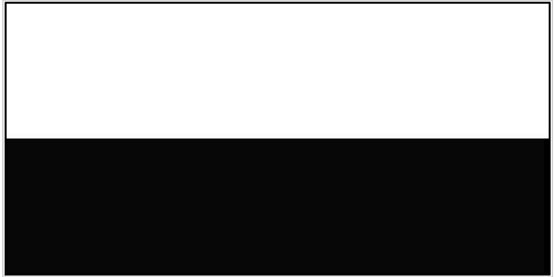
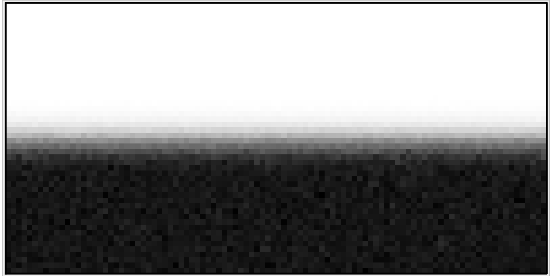
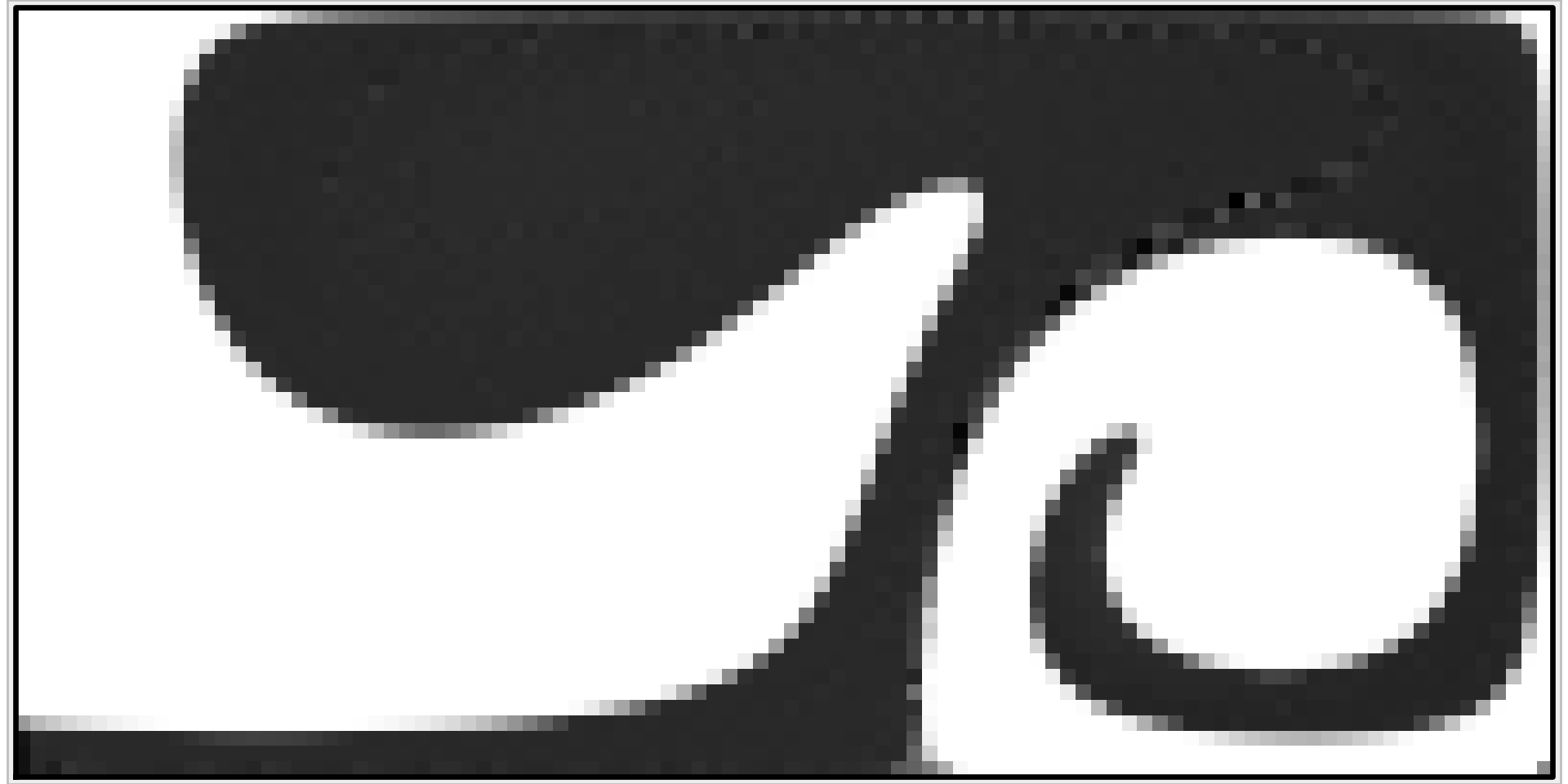
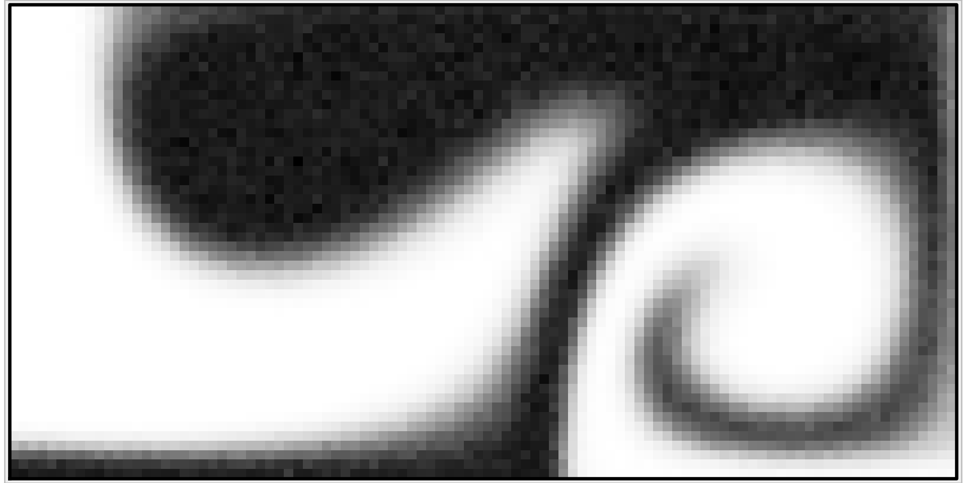
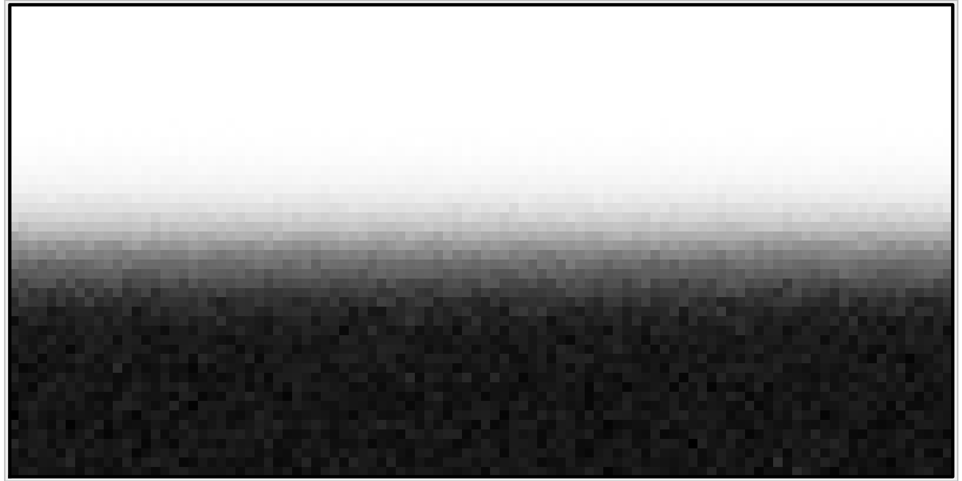
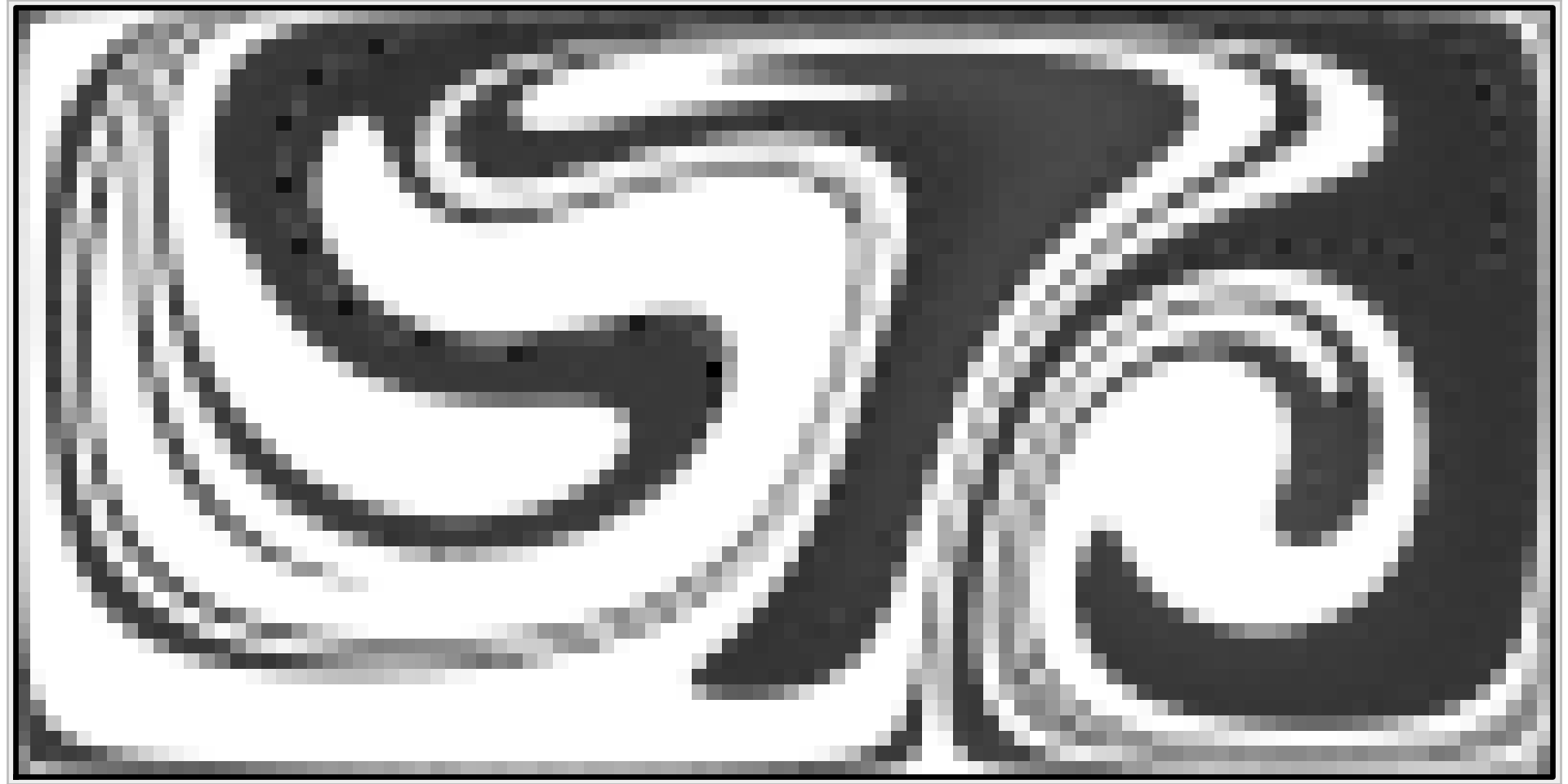
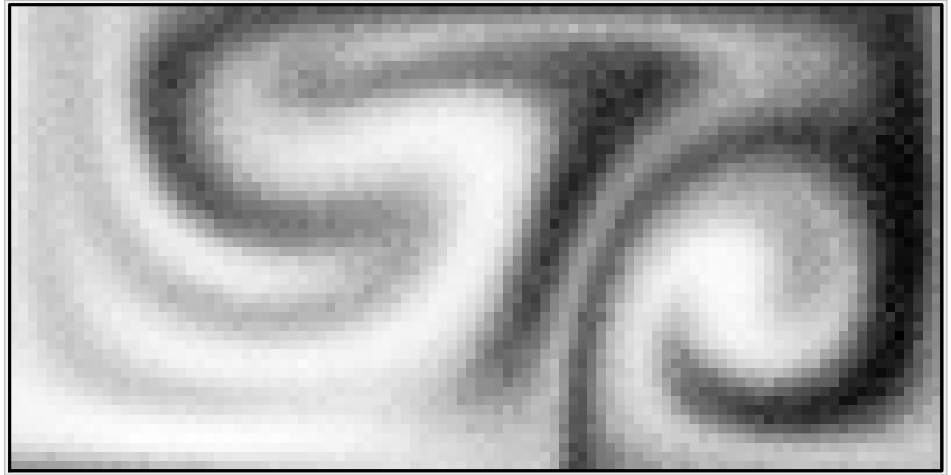
Figure 1: Mixing of a passive tracer, initially located in the bottom half of the domain. In the left column, Fickian diffusion is applied, in the middle column, advection by a double gyre, and in the right column, both advection and diffusion.

While “turbulent mixing” is in reality a combination of stirring by turbulence and molecular diffusion, it will in almost all cases be impractical to model it as such. In particular, eddies in the ocean exist at all scales, from the largest ocean gyres with a scale of several thousand kilometers, to the smallest turbulent eddies at the Kolmogorov scale (Davidson, 2015, p. 25), on the order of 1 mm or less. Most numerical ocean models currently have a horizontal resolution somewhere between 10s of meters and 10s of kilometers, and a vertical resolution ranging from meters to 100s of meters. Any eddies smaller than the resolution of the model cannot be resolved, and therefore their contribution to the mixing must be parameterised, as the so-called eddy diffusivity. When talking about diffusion in the context of oil trajectory modelling, and indeed for the rest of this chapter, one typically refers to the eddy diffusivity.

2.2 Origins of vertical mixing in the ocean

There are many sources of turbulent kinetic energy (TKE) leading to vertical mixing in the ocean. The most obvious (and spectacular) may be breaking waves, which contribute to mixing in the upper part of the water column. Furthermore, turbulent motion may be caused as currents flow across the sea bed, in narrow straits, or due to shear flow between two fluid layers. In cold or windy conditions, evaporation or cooling at the surface will increase the density of the water, and if the water at the surface becomes denser than the underlying water, overturning will occur, leading to vertical mixing. In very cold conditions, sea ice will form. During the freezing process, the salinity of the ice is reduced through rejection of brine. This cold, high-salinity water will have a density higher than the water below, again leading to overturning and mixing of water masses.

In all cases, the stratification of the water column has a strong influence on the vertical diffusivity. Near the surface, there will usually be a layer of uniform density, called the surface mixed layer, or just the mixed layer. The thickness, or depth, of the mixed layer will vary with geographical location, time of year, and it will be influenced by local factors such as wind, air temperature, rainfall and freshwater input from rivers.

While eddy diffusivity is typically high in the interior of the mixed layer, it drops both close to the surface, and towards the bottom of the mixed layer. Towards the surface, the mixing efficiency (which the eddy diffusivity describes), is limited because the surface limits the size of turbulent eddies (Craig and Banner, 1994). This is a version of the so-called mixing length argument (see, e.g., Davidson (2015, pp. 112–113)), stating that the mixing depends not only on the turbulent kinetic energy, but also on the size of eddies.

At the bottom of the mixed layer, the density increases, either due to an increase in salinity, a decrease in temperature, or a combination of both. This region of increasing density is called the pycnocline. Stable stratification, where a layer of light water overlays denser water, will tend to prevent mixing across the density gradient, due to the energy required to lift the dense water against gravity. For this reason, vertical diffusivity can be quite high throughout the mixed layer, and then drop, sometimes by several orders of magnitude, at the pycnocline. The interested reader is referred to Gräwe et al. (2012) for further discussion of this particular case, in the context of Lagrangian particle modelling.

As a side note, one might want to ask if the motion of the sea is actually turbulent. If we make the approximation that the water in the mixed layer behaves as an isolated slab of water, experiencing friction forces from the wind at the top, and from the deep water at the pycnocline, then the Reynolds number (Thorpe, 2005, p. 23) for this flow is

$$\mathrm{Re}=\frac{\Delta uL}{\nu},$$ (2)

where $\Delta u$ is the difference between the speed at the top and the bottom of the mixed layer, $L$ is the thickness of the mixed layer, and $\nu$ is the kinematic viscosity of water, which is approximately $1.4\text{\times}{10}^{-6}\text{\,}\mathrm{m}\text{\,}{\mathrm{}}^{2}\text{/}\mathrm{s}$ for seawater at $10\text{\,}\mathrm{\SIUnitSymbolCelsius}$. Turbulent flow is commonly said to occur at Reynolds numbers above approximately 4000. If we choose for example a mixed layer thickness of $L=$10\text{\,}\mathrm{m}$$, we see that any velocity difference of more than about $0.5\text{\times}{10}^{-3}\text{\,}\mathrm{m}\text{/}\mathrm{s}$ will give turbulent flow.

The above discussion of turbulent flow assumes that the density truly is constant throughout the mixed layer. In regions where the density increases slowly with depth, a relevant parameter to consider is the Richardson number,

$$\mathrm{Ri}=\frac{g}{\rho_{w}}\frac{\frac{\partial\rho_{w}}{\partial z}}{\left(\frac{\partial u}{\partial z}\right)^{2}},$$ (3)

which is a dimensionless number related to the ratio between the stabilising forces of stratification, and the destabilising forces of current shear. If $\mathrm{Ri}\gg 1$, then the shear forces are not strong enough to break down the density gradient and cause vertical mixing.

2.3 Modelling ocean turbulence

The vertical eddy diffusivity can be described through models of different complexity, including simple parametrisations based on fitting simplified models against experiments, and more complex models that try to solve dynamic equations for transport and dissipation of turbulent kinetic energy.

The simplest model for vertical turbulent mixing would be to simulate a vertical advection-diffusion process using a constant eddy diffusivity. However, in light of the discussion in Section 2.2, it should be clear that this will in many cases be too simple. In particular, the diffusivity in the mixed layer can often be several orders of magnitude higher than the diffusivity at greater depths.

Hence, the second simplest approach might be to model the diffusivity profile as a step function, with a high value in the mixed layer, and a lower value below the pycnocline. However, note that care must be taken to avoid numerical artifacts when using a step-function diffusivity. See Sections 7.2 and 7.4 for examples and additional discussion of this topic.

Another approach is to use a simplified continuous model for the vertical diffusivity. One such model, used in some oil spill modelling studies (Skognes and Johansen, 2004; Nordam et al., 2018), is due to Ichiye (1967), who suggested the following relation for the vertical eddy diffusivity as a function of depth ($z$ positive downwards):

$$K(z)=0.028\frac{H_{s}}{T_{p}}\mathrm{e}^{-2kz},$$ (4)

where $H_{s}$ is the significant wave height, $T_{p}$ is the peak wave period, and $k$ is the wave number. This relation takes mixing due to waves into account, but ignores the limiting effects of stratification, and does not feature reduced diffusivity towards the surface.

A third option is to obtain eddy diffusivity from an ocean model. All or most ocean models calculate eddy diffusivity, potentially taking into account waves, density stratification, current shear, and more complex processes such as Langmuir circulation (Thorpe, 2005, pp. 251–255). Several different approaches at different degrees of complexity exist. So-called turbulence closure schemes are a research field in themselves, and we will not go into detail on the schemes themselves here. The interested reader is referred to, e.g., Davidson (2015, p. 27) and Haidvogel and Beckmann (1999, Chapter 5).

Relevant in the context of oil spill modelling is that many ocean models provide eddy diffusivity as output on the same formats as the ocean current data. A three-dimensional oil spill model will probably already be using currents from an ocean model, and the advantage of using eddy diffusivity from the same model is then that the fields are dynamically consistent. However, it is important to be aware that the eddy diffusivity in an Eulerian ocean model also serves the additional purpose of suppressing numerical instabilities that can occur in advection-dominated problems. Hence, it is quite possible that the eddy diffusivity from an ocean model may be somewhat higher than it should be, and therefore unsuited for direct use in a Lagrangian transport model. Never the less, diffusivity from an ocean model would be expected to take the important effects of stratification into account.

Finally, it is worth mentioning the existence of separate, stand-alone models for vertical ocean turbulence. The most well-known of these is probably the General Ocean Turbulence Model (GOTM) (Umlauf et al., 2005). This is an open-source one-dimensional water column model, that can be set up to model a range of different cases, with different forcings as input, and using different turbulence closure schemes, such as Mellor-Yamada (Mellor and Yamada, 1982), $k$-$\epsilon$ (Launder and Spalding, 1983), and $k$-$\omega$ (Wilcox, 2008). In an oil spill modelling context, using a one-dimensional turbulence model is not as convenient as using eddy diffusivity from an ocean model, but might be an option for a localised area.

2.4 Wave modelling

As previously mentioned, breaking waves are a source of turbulent mixing in the ocean. In the context of oil spill modelling, however, breaking waves are perhaps even more important as the mechanism by which an oil slick at the surface is broken up into droplets and submerged in the water column. We will return to this point in Section 3, but here we will mention some approaches to obtain wave data for use in an oil spill model.

As with turbulence, there exists different approaches to obtaining wave data, at different levels of complexity. Advanced wave models that calculate the entire wave spectrum exist, and may be run coupled to an ocean model (or atmosphere-ocean model), such that the waves affect the calculation of the current, and vice versa. An example of such a model is SWAN (Booij et al., 1997), which may for example be coupled with the ROMS ocean model (see, e.g., Warner et al. (2008)).

A simpler approach is to parameterise the wave state from the wind speed, usually given at an altitude of 10 m above sea level. In the following example, the significant wave height, and the peak wave period, $H_{s}$ and $T_{p}$, are derived from the JONSWAP spectrum and associated empirical relations (Carter, 1982). The sea state is assumed to be either fetch-limited, or fully developed. Fetch-limited means that a steady state is reached, where the sea does not reach a fully developed state because the fetch (the distance over which the wind acts on the sea) is too short. This is relevant close to the coast, in off-shore wind conditions. Fully developed, on the other hand, refers to the steady state wave conditions that are found far away from the coast. In both cases, the wave state is assumed not to be time-limited, i.e., the wind is assumed to have been constant for a sufficiently long time to allow a steady wave state to develop.

Here, $H_{s}$ and $T_{p}$ are given by

$$H_{s} =\frac{u_{10}^{2}}{g}H_{c}\sqrt{\frac{gL_{f}}{u_{10}^{2}}}$$ (5a)

$$T_{p} =\frac{u_{10}}{g}T_{c}\sqrt[3]{\frac{gL_{f}}{u_{10}^{2}}}$$ (5b)

in the fetch-limited case, and

$$H_{s} =\frac{u_{10}^{2}}{g}H_{0}$$ (6a)

$$T_{p} =\frac{u_{10}}{g}T_{0}$$ (6b)

in the fully developed case. Here, $H_{0}=0.243$, $H_{c}=0.0016$, $T_{0}=8.134$, and $T_{c}=0.286$ are dimensionless parameters, $g$ is the gravitational acceleration, $L_{f}$ is the fetch length, and $u_{10}$ is the wind speed at 10 m above sea level.

3 Entrainment of surface oil

When a wave breaks on an oil slick, part of the oil in the breaking zone of the wave will be entrained into the water column in the form of droplets. The amount of entrained oil will increase with the height of wind-driven waves, and therefore depends on the wind speed. To describe this in an oil spill model it is necessary to formulate a model for the mass of oil entrained per unit of time for a given surface slick in a given wave field. Some of the earliest quantitative work on the entrainment of oil due to breaking waves is that of Delvigne and Sweeney (1988). In this classic paper, based on experiments in a turbulence tank and two different meso-scale wave flumes ($0.43\text{\,}\mathrm{m}$ and $4.3\text{\,}\mathrm{m}$ depth), they provided empirical relations for the three key parameters in surface oil entrainment:

• Droplet size distribution of the entrained oil,

• Entrainment rate,

• Intrusion depth.

The relationships obtained by Delvigne and Sweeney (1988) were used for decades in oil spill models, with new models only starting to take hold nearly thirty years later. The empirical relationship for entrainment rate by Delvigne and Sweeney was formulated in a convoluted way, where the entrainment rate depends on the droplet size distribution, and the models lack theoretical support. These and other aspects of the Delvigne and Sweeney models have been critisised by others who have formulated alternative models in recent years (Johansen et al., 2015; Li et al., 2017c).

3.1 Droplet size distribution of entrained oil

After entrainment of a surface slick, smaller droplets take longer to resurface compared to larger droplets (see Section 4.1). For this reason, the droplet size distribution of entrained oil is an important factor that influences both the horizontal transport of the oil, and the lateral dispersion from current shear. To describe dispersion, it is therefore necessary to use an accurate droplet size model. Experimental evidence has shown that the size distribution of droplets in a breaking wave event depends on oil viscosity (Delvigne and Sweeney, 1988; Reed et al., 2009), oil-water interfacial tension (Zeinstra-Helfrich et al., 2016; Li et al., 2017a), oil film thickness (Zeinstra-Helfrich et al., 2016, 2015), and energy in the breaking wave (Delvigne and Sweeney, 1988). Several published models exist which use these and other parameters to estimate a droplet size distribution (Delvigne and Sweeney, 1988; Reed et al., 2009; Zhao et al., 2014; Johansen et al., 2015; Li et al., 2017b; Nissanka and Yapa, 2017).

Two main droplet size model types can be distinguished. One type is an equilibrium description, where the model consists of an expression for a characteristic droplet size, such as the median, and a static droplet size distribution function, such as a Rosin-Rammler, log-normal, or power-law function, each with associated distribution parameters (Delvigne and Sweeney, 1988; Reed et al., 2009; Johansen et al., 2015). This formulation gives a static distribution representative for some depth and after some time of wave impact. The other type of formulation aims to calculate a dynamic droplet size distribution through population balance models, which describe the time-evolution of droplet breakup and coalescence in turbulent flow after wave breaking (Zhao et al., 2014; Nissanka and Yapa, 2016). The equilibrium type model is conceptually simpler and is easier to implement in an oil spill model, while the population balance model may offer a more detailed description of the physical process of droplet breakup. As of today, it is not clear which approach is best for oil spill modelling.

In the following, the equilibrium type droplet size model of Johansen et al. (2015) will be described. This model is formulated from the observation that there are two main regimes that determine the droplet size of oil in turbulent flow; a viscosity-limited regime and an interfacial tension-limited regime. The first regime is representative for weathered and emulsified surface oil, while the second regime is representative for oil that has been treated with chemical dispersants. Each regime is associated with the characteristic droplet size through a non-dimensional number found from dimensional analysis. The interfacial tension-limited regime is associated with the Weber number and the viscosity-limited regime with the Reynolds number.

The Weber number is

$$\mathrm{We}=\frac{v^{2}\rho_{o}h}{\sigma_{ow}},$$ (7)

where $\rho_{o}$ is the density of the oil, $\sigma_{ow}$ is the oil-water interfacial tension, $h$ is the surface slick thickness, and $v=\sqrt{2gH}$ a velocity scale related to the wave motion, with $H$ being the wave height.

The Reynolds number is given by

$$\mathrm{Re}=\frac{v\rho_{o}h}{\mu_{o}},$$ (8)

where $\mu_{o}$ is the dynamic viscosity of the oil.

Assuming that the characteristic droplet size can be found through a scaling relationship involving these two numbers, in addition to three constants to be determined from fitting to data, the ratio of characteristic droplet size $D$ to slick thickness $h$ with the Reynolds and Weber numbers was found as

$$\frac{D}{h}=A\mathrm{We}^{-a}\left[1+B^{\prime}\left(\frac{\mathrm{We}}{\mathrm{Re}}\right)^{a}\right]$$ (9)

The constants $A$, $B^{\prime}$ and $a$ appearing in this equation were fit to experimental data in Johansen et al. (2015) as $A=2.251$, $B^{\prime}=0.027$ and $a=0.6$.

Equation (9) provides a prediction for a characteristic droplet size of the droplet size distribution. This can in principle be any characteristic size and any distribution formulation; in Johansen et al. (2015) these were taken to be the median of the droplet size number distribution, which was described through a log-normal function. In oil spill modelling, the volume distribution for droplet sizes is needed, in order to account for the mass of oil. From the log-normal distribution, one can obtain the volume distribution from the number distribution by shifting the distribution as described in Johansen et al. (2015). Specifically, the volume droplet size distribution (for diameter $d$) is given as

$$v(d) =\frac{1}{d\sqrt{2\pi}\sigma}\exp\left[-\frac{(\ln d-\mu)^{2}}{2\sigma^{2}}\right]$$ (10)

where we use a logarithmic standard deviation of $\sigma=0.4\,\ln(10)$. The logarithmic mean $\mu$ is given by $d^{v}_{50}=\mathrm{e}^{\mu}$, and the relationship between the volume and number median diameters is

$$\ln(d^{v}_{50})=\ln(d^{n}_{50})+3\sigma^{2}.$$ (11)

A similarly formulated model is the one of Li et al. (2017b), which is a droplet size distribution model intended to be valid for both surface entrainment by breaking waves, and subsea blowouts through an orifice. In this model, the maximum stable droplet size due to the Rayleigh-Taylor instability is used as a length scale parameter, instead of the surface oil film thickness. Avoiding the surface oil film thickness means that no separate model is needed to calculate this value dynamically. At the same time, experimental evidence shows that characteristic droplet size does scale with oil film thickness (Zeinstra-Helfrich et al., 2016), making it an experimentally validated predictor, although it should be noted that earlier work did not find a clear relationship between the two variables (Delvigne and Sweeney, 1988).

3.2 Entrainment rate of oil due to breaking waves

Historically, entrainment rate was explicitly or implicitly coupled to droplet size distribution. One made the distinction between larger oil droplets that almost immediately resurfaced after entrainment, and smaller droplets, that became “permanently entrained” (see, e.g., Reed et al. (1999) and references therein). The net entrainment rate would then only include the permanently entrained oil.

Delvigne and Sweeney (1988, Section 4.4) found an expression for the entrainment rate that explicitly included the droplet size:

$$Q(d)=C\cdot D^{0.57}_{ba}S_{cov}F_{wc}d^{0.7}\Delta d,$$ (12)

where $D_{ba}$ is the dissipated energy per surface area [$\text{\,}\mathrm{J}\text{\,}{\mathrm{m}}^{-2}$], $S_{cov}$ is the sea surface area fraction covered by oil, $F_{wc}$ is the sea surface area fraction hit by breaking waves per second [$\text{\,}{\mathrm{s}}^{-1}$], $d$ is the droplet size [$\text{\,}\mathrm{m}$] and $\Delta d$ is the width of the droplet size interval (centered on $d$). The prefactor $C$ is an empirical constant that can include the effects of oil state, such as viscosity, interfacial tension, and density; in Delvigne and Sweeney (1988) only viscosity is included for different values of $C$.

It is not explicitly stated in the original work of Delvigne and Sweeney (1988) how this equation should be applied to calculate the total entrainment rate; it has however been interpreted in the literature (Li et al., 2017b). The equation gives the entrainment rate over a droplet size interval, which means that an integration over size intervals must be performed. This means that a lower and upper limit of the droplet size must be decided upon. It is likely that different interpretations of Eq. (12) exist, meaning that models using this equation differently will provide somewhat different results.

From a modelling point of view, a more elegant solution is to have an expression of the entrainment rate that is completely independent of the droplet size distribution, and heuristic concepts such as “permanently dispersed oil”. Johansen (1982) describes such an approach, modelling the vertical transport (rise due to buoyancy, and vertical mixing due to eddy diffusivity) with the advection-diffusion equation. He points out that in order to represent a distribution of droplet sizes (and thus a distribution of rise speeds), one must solve the advection-diffusion equation for each size class.

In such a model, the entrainment rate describes the amount of oil that is submerged, and the droplet size distribution will describe how that oil is distributed across size classes. The vertical transport model will then determine the future development of those droplets, allowing large droplets to surface rapidly, while small droplets remain submerged for longer periods.

Recent formulations of the entrainment rate adhere to this principle. Both the two following examples describe the submersion of surface oil as a first-order decay process

$$\frac{\mathrm{d}Q_{s}}{\mathrm{d}t}=-\alpha Q_{s},$$ (13)

where $Q_{s}$ is the amount of oil at the surface, and $\alpha$ is the entrainment rate. Johansen et al. (2015) describe a simple model where the submersion of surface oil is related to the white-cap coverage fraction, $f_{wc}$ and the mean wave period, $T_{m}$:

$$\alpha=Pf_{wc}/T_{m}.$$ (14)

In Johansen et al. (2015), Eq. (14) was used as a standalone model to describe the development of oil mass on the surface. It was thus assumed that droplets larger than some limiting diameter would resurface directly, and $P$ was then taken to be the fraction of droplets smaller than this limiting diameter. For use in a modelling system where a vertical transport model determines the fate of the droplets, we assume that oil is entrained at the full rate, setting $P=1$. Then, the transport model will allow the larger droplets to surface quickly.

Li et al. (2017b) developed an empirical relation parameterising the entrainment rate, $Q$, in terms of the dimensionless Weber and Ohnesorge numbers:

$$\frac{Q}{F_{bw}}=a\mathrm{We}^{b}\mathrm{Oh}^{c}.$$ (15)

Here, $F_{bw}$ is the white-capping fraction per unit time [s^-1], the Weber number is $\mathrm{We}=d_{o}\rho_{w}gH_{s}/\sigma_{ow}$, where $\rho_{w}$ is the density of water, and the Ohnesorge number is $\mathrm{Oh}=\mu_{o}/\sqrt{\rho_{o}\sigma_{ow}d_{o}}$. The length scale is the Rayleigh-Taylor instability maximum droplet diameter, given by

$$d_{o}=4\left(\frac{\sigma_{ow}}{(\rho_{w}-\rho)g}\right)^{1/2}.$$ (16)

The values of the empirical parameters are $a=4.604\times 10^{-10}$, $b=1.805$, and $c=-1.023$ (Li et al., 2017b).

3.3 Entrainment depth of oil due to breaking waves

The linear parameterisation of intrusion depth and distribution of oil found by Delvigne and Sweeney (1988) is that after a wave breaking event, the oil is distributed evenly in the interval

$$(1.5-0.35)H_{w}<z<(1.5+0.35)H_{w},$$ (17)

where $H_{w}$ is the wave height. No more recent general model formulations for the intrusion depth have been published in the oil spill literature. However, in disagreement with this model, recent experiments in a wave tank gave intrusion depth centers of less than half the wave height (Li et al., 2017a). Other work that may be relevant in this context includes studies of bubble entrainment by breaking waves (see, e.g., Leifer and De Leeuw (2006)) and observations of vertical distributions of buoyant fish eggs (see, e.g. Röhrs et al. (2014)).

4 Submerged oil

The vertical transport processes that affect submerged oil droplets are rise due to buoyancy (or sinking in some cases, see, e.g., King et al. (2014)), turbulent mixing, and vertical advection by currents. Of these three, advection by vertical currents is probably the least important. Hence, we will not discuss this further, other than to state that if current data with a vertical current component is available, it can be used to advect the oil, just like the horizontal components.

Vertical turbulent mixing has already been discussed in Section 2.3, and how to use the eddy diffusivity in an oil spill model will be discussed in Sections 5 and 6. Hence, the main content of this section will be the calculation of rise speeds for oil droplets.

4.1 Calculation of droplet rise speeds

It is commonly assumed that droplets, bubbles, sediment particles, etc. rise or sink at their terminal velocity. The terminal velocity is derived by starting from the observation that buoyancy exerts a constant force, $F_{b}$, on the submerged particle:

$$F_{b}=\frac{4}{3}\pi r^{3}g(\rho_{a}-\rho_{p})=\frac{4}{3}\pi r^{3}\rho_{a}g^{\prime},$$ (18)

where $g^{\prime}=g\frac{\rho_{a}-\rho_{p}}{\rho_{a}}$ is the reduced gravity, with $\rho_{a}$ and $\rho_{p}$ the density of the ambient fluid and the moving particle, respectively. While the buoyancy is constant, the drag force, $F_{D}$, increases with the velocity, and has direction opposite to the velocity:

$$F_{D}=-\frac{1}{2}\rho_{a}v^{2}C_{D}A\cdot\frac{v}{|v|},$$ (19)

where $v$ is the velocity of the particle relative to the fluid, $A$ is the cross-sectional area of the particle, and $C_{D}$ is a drag coefficient. By setting the total force equal to 0, we get an equation that can be solved to find the terminal speed, $v_{b}$:

$$v_{b}=\sqrt{\frac{4}{3}\frac{dg^{\prime}}{C_{D}}}.$$ (20)

The drag coefficient, $C_{D}$, is not constant, but rather a function of the Reynolds number, which for a sphere is given by

$$\mathrm{Re}=\frac{vd}{\nu_{a}}=\frac{\rho_{a}vd}{\mu_{a}}.$$ (21)

Here, $v$ is the speed of the sphere, $d$ is the diameter of the sphere, and $\nu_{a}$ and $\mu_{a}$ are the kinematic and dynamic viscosities of the surrounding fluid, and $\rho_{a}$ is its density.

At low Reynolds numbers, $\mathrm{Re}\ll 1$, the drag coefficient is given by

$$C_{D}=\frac{24}{\mathrm{Re}}.$$ (22)

With this drag coefficient, the expression for the drag force becomes

$$F_{D}=-6\pi r\mu_{a}v.$$ (23)

Solving for the terminal speed, $v_{b}$, one obtains

$$v_{b}=\frac{2}{9}\frac{\rho_{p}-\rho_{a}}{\mu_{a}}gr^{2}.$$ (24)

Equation (23) for the drag force is commonly known as Stokes’ law, after George Gabriel Stokes (Stokes, 1856), although Eqs. (22) and (24) are also sometimes referred to as Stokes’ law.

In the derivation of Stokes’ law, an assumption was made that the flow around the spherical particle is laminar. At higher Reynolds numbers, the flow around the sphere is no longer laminar, and Stokes’ law no longer holds. Various empirical formulae exist for the case of high Reynolds number. Clift et al. (1978) combined several previously published results, and developed a piecewise parameterisation of $C_{D}$ as a function of the Reynolds number, which they call the Standard Drag Curve for the drag coefficient of a spherical particle (Clift et al., 1978, pp. 110–112). This parameterisation is shown in Fig. 2, together with Stokes’ law (Eq. (22)) and two other parameterisations.

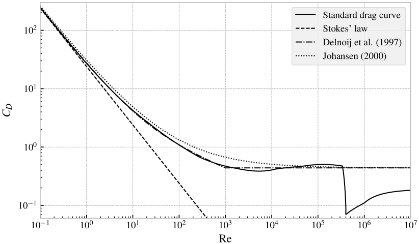
Figure 2: Parameterisation of the Standard Drag Curve, due to Clift et al. (1978). Stokes’ law, which is valid for $\mathrm{Re}\ll 1$, is shown as a dashed line.

As the highest range of Reynolds numbers in Fig. 2 is not relevant for oil droplets rising due to buoyancy, simpler expressions than the standard drag curve have been suggested. Delnoij et al. (1997) suggested a parameterisation of $C_{D}$ given by

$$C_{D}=\left\{\begin{array}[]{lll}\frac{24}{\mathrm{Re}}(1+0.15\mathrm{Re}^{0.687})&\mathrm{if}&\mathrm{Re}<1000\\ 0.44&\mathrm{if}&\mathrm{Re}\geq 1000\end{array}\right..$$ (27)

Johansen (2000) proposed a variant of the above scheme where the terminal rise velocity is instead given by a harmonic transition between the high and low Reynolds number cases:

$$v_{b}=\left(\frac{1}{v_{1}}+\frac{1}{v_{2}}\right)^{-1},$$ (28)

where $v_{1}$ and $v_{2}$ are calculated from Eq. (20), with a drag coefficient of $C_{D}=24/\mathrm{Re}$ in $v_{1}$, and $C_{D}=0.44$ in $v_{2}$. The parameterisations due to Delnoij et al. (1997) and Johansen (2000) are also shown in Fig. 2·

All of the above expressions assume spherical particles. In reality, an oil droplet rising through water will deform to some degree, depending among other things on the volume, density and oil-water interfacial tension. Work on this topic includes that of Bozzano and Dente (2001), which takes droplet deformation into account. They developed empirical relations for the drag coefficient and deformation of droplets and bubbles in terms of the Reynolds, Morton and Eötwös numbers:

$$C_{D} =f\left(\frac{a}{R_{0}}\right)^{2},$$ (29a)

where

$$f =\frac{48}{\mathrm{Re}}\left(\frac{1+12\mathrm{Mo}^{1/3}}{1+36\mathrm{Mo}^{1/3}}\right)+0.9\frac{\mathrm{Eo}^{3/2}}{1.4(1+30\mathrm{Mo}^{1/6})+\mathrm{Eo}^{3/2}},$$ (29b)

$$\left(\frac{a}{R_{0}}\right)^{2} =\frac{10(1+1.3\mathrm{Mo}^{1/6})+3.1\mathrm{Eo}}{10(1+1.3\mathrm{Mo}^{1/6})+\mathrm{Eo}},$$ (29c)

and the Morton and Eötwös numbers are given by

$$\mathrm{Mo}=\frac{g\mu_{a}^{4}(\rho_{a}-\rho_{p})}{\rho_{a}^{2}\sigma^{3}},\;\;\;\;\mathrm{Eo}=\frac{gd_{0}^{2}(\rho_{a}-\rho_{p})}{\sigma}.$$ (29d)

Here, $\sigma$ is the interfacial tension between oil (or gas) and water, and $d_{0}$ is the equivalent diameter of of the particle, i.e., the diameter of a sphere with the same volume.

4.2 Role of dispersants

Oil dispersants are specifically designed surfactant chemicals intended to reduce the oil-water interfacial tension. Dispersants can be used as a countermeasure during oil spill response, with the objective of enhancing the dispersion of the spill by facilitating the creation of small oil droplets. This can be done subsea during a blowout, where the dispersants are injected directly into the oil stream, facilitating breakup of the oil into smaller droplets in the turbulent jet, or it can be done at the surface, where the treated oil will be broken up into small droplets when hit by breaking waves or other mechanical energy.

Looking at Eqs. (7) and (9), we see that reduced interfacial tension gives a larger Weber number, which in turn gives a smaller characteristic droplet size in natural dispersion, when everything else is kept constant. While droplet breakup in turbulent jets is outside the scope of this chapter, we can briefly mention that also in this case the droplet size be may related to the Weber number, and reduced interfacial tension with everything else kept constant will lead to smaller droplets (Brandvik et al., 2013; Johansen et al., 2013).

Small droplets produced by dispersant application will have a slower rice velocity, as discussed earlier in this chapter. As also mentioned, this will lead to the oil being spread over a larger volume of water, due to current shear and horizontal transport and mixing. Smaller droplets give rise to faster dissolution and faster biodegradation of the oil, potentially decreasing the overall lifetime of contamination after the spill. However, one should also be aware that applying dispersants does not remove the oil, even if it is less visible. Dispersant application can reduce the potential impact to sea birds, mammals, and shoreline habitats, but at the cost of potentially increasing the impact on marine life in the water column, as well as benthic species.

5 Eulerian model of vertical mixing

Calculating in the Eulerian picture means to consider concentrations at a set of points (or in a set of cells), and looking at how the concentrations in those points change with time. Solving a partial differential equation (PDE), such as the advection-diffusion equation, for a discrete grid of points, is an example of an Eulerian calculation. For different reasons, which will be described in more detail in Section 6, it is not very common to solve oil spill problems in the Eulerian picture. Nevertheless, some background information on the Eulerian picture is very useful, as this forms the starting point for the Lagrangian, particle based approach of oil spill modelling.

5.1 Advection-diffusion equation

The change in concentration, along the vertical dimension, of oil droplets that rise due to buoyancy and are mixed due to ocean turbulence, is commonly modelled as an advection-diffusion problem. Assuming the droplets to rise with a constant, terminal velocity, $v_{b}$, and that the spatially dependent diffusivity can be expressed as a function of depth and time, $K(z,t)$, the concentration of droplets as a function of space and time, $C(z,t)$, is described by

$$\frac{\partial C}{\partial t}=\frac{\partial}{\partial z}\left(K\frac{\partial C}{\partial z}\right)-v_{b}\frac{\partial C}{\partial z}.$$ (30)

If we have $v_{b}=0$ and $K(z,t)>0$, then this equation is simply the diffusion equation (also known as the heat equation). For simple geometries and initial conditions, analytical solutions are known for many cases, in particular if $K(z,t)$ is a constant (see e.g., Carslaw and Jaeger (1959)) With $v_{b}\neq 0$ and $K(z,t)=0$, Eq. (30) becomes the advection equation, which describes the transport of a concentration profile, without diffusion. For the special case of constant $v_{b}$, the advection equation in one dimension describes a concentration profile that moves at a speed of $v_{b}$, without changing its shape.

For practical applications, it is usually not possible to find analytical solutions to Eq. (30). In such cases, a range of numerical solution techniques exist. For details, the interested reader is referred to the wide range of literature on the topic of numerical solutions of PDEs. See, e.g., Hundsdorfer and Verwer (2003); Versteeg (2007); Pletcher (2013).

5.2 Boundary conditions

In oil spill modelling, it is essential to distinguish between surface oil and submerged oil. Surface oil is not only distinguished by being located at zero depth, but also by the fact that surface oil is not subject to vertical mixing due to turbulence in the water column. The idea behind this is that submerged oil are found in the form of droplets, which are surrounded by water and thus subject to turbulent motion. Surface oil, on the other hand, is present in the form of continuous patches of different sizes. In order to submerge oil from a patch or slick at the surface, some high-energy event, such as a breaking wave, is required to break the surface tension of the oil. The opposite process, i.e., surfacing, is usually calculated from the buoyant rise speed of the oil droplets. Oil that reaches the surface due to buoyancy may leave the water column and merge with the surface slick. This makes oil behave differently than, e.g., buoyant fish eggs, as these do not “get stuck” at the surface in the same way (Sundby and Kristiansen, 2015).

One way to model this behaviour of oil is to assume that the concentration in the water column is described by the advection-diffusion equation, with a partially absorbing boundary at the surface. In particular, the boundary at the surface should enforce zero diffusive flux, while allowing the advective flux due to buoyancy to leave the water column through the boundary at the surface. The oil that has left the water column in this manner is then counted as part of the surface oil. The physical rationale for this choice of boundary conditions is that higher buoyancy (due to either larger droplets or less dense oil) does lead to faster surfacing, while higher diffusivity does not lead to faster surfacing.

The advective and diffusive fluxes are given by:

$$j_{A}(z,t) =wC(z,t),$$ (31a)

$$j_{D}(z,t) =-K(z,t)\frac{\partial C(z,t)}{\partial z},$$ (31b)

where Eq. (31b) is commonly known as Fick’s law (see, e.g., Csanady (1973, p. 4)). Hence, a no-diffusive-flux boundary condition at $z=0$ can be enforced by requiring

$$\left.\frac{\partial C(z,t)}{\partial z}\right|_{z=0}=0.$$ (32)

Another option for modelling the surfacing of oil is to consider the surfacing process as a loss term in the PDE (also known as a sink), where oil which is sufficiently close to the surface is simply removed, at a rate which would typically be calculated from the rise speed of the oil droplets. See, e.g., Tkalich and Chan (2002) for an example of this approach. Note that the same rate of surfacing can be modelled in both approaches.

When considering a finite water depth, the boundary at the bottom should also be reflecting for the diffusion step. As long as the oil considered is positively buoyant, the advective flux through the bottom will necessarily remain zero. In advanced oil spill models, interaction with seabed sediments of different types through a turbid bottom layer may be included, where adhesion of oil to sediments is explicitly modelled. One may also wish to account for the possibility of sinking droplets of oils that are denser than water settling onto the sediment.

5.3 Source term for entrainment of oil

In the scheme described above, the concentration of submerged oil in the water column is described by the advection-diffusion equation (Eq. (30)). In this case, we may model the entrainment of oil by adding a reaction term to Eq. (30), which adds oil at certain depths. For example, if oil is entrained at rate $Q(t)$ (units mass per time), and distributed evenly across a depth interval ranging from $H_{min}$ to $H_{max}$, we have

$$\frac{\partial C}{\partial t}=\frac{\partial}{\partial z}\left(K(z)\frac{\partial C}{\partial z}\right)-v_{b}\frac{\partial C}{\partial z}+R(z,t),$$ (33a)

where

$$R(z,t)=\left\{\begin{array}[]{ccc}Q/L&\mathrm{if}&H_{min}<z<H_{max}\\ 0&\mathrm{otherwise}\end{array}\right.,$$ (33d)

where $L=H_{max}-H_{min}$.

5.4 Modelling a droplet size distribution

An important point in oil spill modelling is the concept of a droplet size distribution, as discussed in Section 3.1. As oil is submerged due to breaking waves, a range of droplet sizes are produced, and these will have a different fate in the water column. Not only does the droplet size strongly influence the rise speed (see Section 4.1), but also dissolution and biodegradation are affected by the droplet size, due to the change in surface area relative to volume.

To capture the effect of droplet size on rise velocity in an Eulerian model, one needs to separate the submerged oil into discrete droplet size classes, and solve one advection-diffusion equation for each size class. No exchange between droplet size classes is necessary for the submerged oil, but the source term (Eq. (33d)) must be modified such that the correct proportion of the submerged oil is inserted into each size class (Kristiansen et al., 2020).

5.5 The well-mixed condition

The well-mixed condition (WMC), described by Thomson (1987), states that a passive (i.e., neutrally buoyant) tracer that is initially well mixed, must remain well mixed while undergoing diffusion. This holds regardless of the shape of the diffusivity profile, and provided of course that the tracer cannot escape through domain boundaries or similar. The well-mixed condition follows directly from the diffusion equation for a concentration, $C(z,t)$:

$$\frac{\partial C}{\partial t}=\frac{\partial}{\partial z}\left(K(z)\frac{\partial C}{\partial z}\right).$$ (34)

If $\partial_{z}C(z,t)=0$ everywhere (including at the boundaries), then the right-hand side of Eq. (34) is 0, and hence there will be no change in concentration as time passes.

In Eulerian modelling of diffusion, it is fairly straightforward to ensure that the WMC is satisfied. In Lagrangian modelling, on the other hand, this is not always trivial. However, as stated by Thomson (1987), the WMC is a necessary (though not sufficient) condition for a Lagrangian scheme to be consistent with the diffusion equation. We will return to this point in Section 6.

6 Lagrangian modelling of vertical mixing

In oil spill modelling, the most common approach to simulating the transport and mixing of oil at sea is to represent the oil as numerical particles, also called Lagrangian elements (or sometimes “spillets”). These numerical particles move with the current, rise or sink according to their buoyancy, and move randomly to account for turbulent mixing. When a large number of Lagrangian elements is simulated, their distribution may be used to approximate the concentration field of a substance, such as oil.

In this section, we describe some of the theory behind the use of particles to model an advection-diffusion problem, and some conditions that must be satisfied in order for this approach to be equivalent to the Eulerian approach described above. We also give numerical schemes for the transport and mixing, the boundary conditions, and the entrainment.

The link between the diffusion equation, and the distribution of a collection of randomly moving particles, has been known for a long time. More than 100 years ago, Einstein (1905) showed that the random motion of Brownian particles (e.g., tiny pollen grains suspended in water) caused them to spread out in accordance with the diffusion equation on long time scales. A few years later, Langevin (1908) presented a differential equation for the movement of Brownian particles, based on Newton’s second law with a stochastic force term.

Since then, the mathematical field of stochastic differential equations has been developed further, and put these results on a more solid theoretical foundation. In the following, we shall only use a few elements of the theory of stochastic differential equations, but references to further reading will be given where relevant.

6.1 Modelling vertical diffusion as a random walk

Diffusion in a Lagrangian model is described by a random walk, i.e., a random displacement of particles at each timestep. More formally, a random walk is an example of a Stochastic Differential Equation (SDE), which is a differential equation that includes one or more random terms. A general one-dimensional SDE with one noise term is written

$$\mathrm{d}z=a(z,t)\,\mathrm{d}t+b(z,t)\,\mathrm{d}W_{t},$$ (35)

where $a(z,t)$ is called the drift term, $b(z,t)$ is called the diffusion term or noise term, and $\mathrm{d}W_{t}$ are the random increments of a standard Wiener process, $W(t)$ (Kloeden and Platen, 1992, p. 40).

To solve this equation numerically, we first introduce a discrete time,

$$t_{n}=t_{0}+n\Delta t,$$ (36)

and then we seek a scheme to calculate the next position, $z_{n+1}$, given the position, $z_{n}$, at time $t_{n}$. Numerous numerical schemes for SDEs exist, the simplest of which is the Euler-Maruyama scheme (Maruyama, 1955; Kloeden and Platen, 1992, p. 305). In this scheme, the iterative procedure for integrating Eq. (35) reads

$$z_{n+1}=z_{n}+a(z_{n},t_{n})\,\Delta t+b(z_{n},t_{n})\,\Delta W_{n},$$ (37)

where $z_{n}$ is the position at time $t_{n}$, and $\Delta W_{n}$ is a random number drawn from a Gaussian distribution with zero mean, $\langle\Delta W\rangle=0$, and variance $\langle\Delta W^{2}\rangle=\Delta t$.

For our purposes, it can be shown that if one solves the following SDE for a large number of particles,

$$\mathrm{d}z=(w+K^{\prime}(z))\,\mathrm{d}t+\sqrt{2K(z)}\,\mathrm{d}W(t),$$ (38)

then their distribution will develop according to the advection-diffusion equation (Eq. (30)), with advection $w$, and diffusivity $K(z)$. Additionally, in Eq. (38),

$$K^{\prime}(z)=\left.\frac{\partial K}{\partial z}\right|_{z}.$$ (39)

See A for details on how to derive Eq. (38) from Eq. (30).

If we let the advection term be equal to the rise speed due to buoyancy, $w=v_{b}$, and discretise Eq. (38) with the Euler-Maruyama scheme, we obtain

$$z_{n+1}=z_{n}+\big{(}v_{b}+K^{\prime}(z_{n})\big{)}\,\Delta t+\sqrt{2K(z_{n})}\,\Delta W_{n}.$$ (40)

This equation is a discrete formulation of the transport equation for numerical particles. A similar expression may be used for the horizontal directions. Some variant of this equation is commonly seen in papers on numerical oil spill modelling. Note, though, that it is also quite common to see this equation without the term $K^{\prime}(z_{n})\,\Delta t$, in which case it is not consistent with the advection-diffusion equation (except in the special case where $K$ is a constant). See Section 7.1 for further details.

Just as for Ordinary Differential Equations (ODEs), a range of different numerical schemes exist for solving SDEs such as Eq. (38). For a review of several different schemes in the context of marine particle transport, see e.g., Gräwe (2011); Gräwe et al. (2012). The interested reader should also refer to the generel SDE literature such as the classic work by Kloeden and Platen (1992). See also Section 9.1.

Note that by describing the theory for vertical transport separately, we have implicitly assumed that the vertical motion can be treated independently of the horizontal motion, at least within a timestep. This is usually a fair assumption, as discussed in the next section. However, for a more general treatment, including iso- and diapycnal diffusivity (which leads to a non-diagonal diffusivity tensor, $\mathbf{K}$, if the isopycnals are not horizontal), see Spivakovskaya et al. (2007b).

6.2 Vertical timestep

Regarding the choice of timestep, it will in many cases make sense to have a far shorter timestep for the vertical motion in an oil spill model, than for the horizontal motion. Among the reasons for this is that available ocean data usually have a far higher resolution in the vertical direction than in the horizontal, and that diffusivity gradients tend to be both sharper and more persistent in the vertical direction. Hence, inaccuracies in the vertical transport step can lead to systematic errors in the vertical distribution of oil, which in turn can lead to errors in, e.g., the prediction of surface signature. See Section 7 for some relevant examples.

Visser (1997) wrote down a criterion for the length of the timestep, which is based on the requirement that the diffusivity profile should be approximately linear over the typical length of a random step. If this criterion is satisfied, the well-mixed condition (see Section 5.5) should be reasonably well satisfied. He obtained

$$\Delta t\ll\min\left|\frac{1}{K^{\prime\prime}(z)}\right|$$ (41)

where the minimum is to be taken over the entire water column, and $K^{\prime\prime}(z)$ is the second derivative of $K(z)$ with respect to $z$. (Note that Visser did not take the absolute value, but this is clearly an omission since $K^{\prime\prime}(z)$ can be negative.) According to (Gräwe et al., 2012, Section 3.4), it is commonly agreed that the timestep should be at least one order of magnitude smaller than the limit in Eq. (41).

It is worth noting that if $K^{\prime\prime}(z)$ is not finite everywhere, for example because $K(z)$ is a step function, or is a piecewise linear function with discontinuous first derivative, then the Visser timestep condition can never be satisfied. Fundamentally, this problem stems from the fact that the equivalence between the advection-diffusion equation and the random walk described by Eq. (38), requires both the drift and diffusion coefficients in Eq. (38) to be continuous. See A for further details.

6.3 Boundary conditions

As was discussed in Section 5.2, it is common in oil spill modelling to treat the boundary at the surface differently for diffusion and advection (advection here refers to the buoyant rise of droplets). In a Lagrangian model, this is straightforward to achieve by separating the advection term and the diffusion term in Eq. (38) into two separate steps. During each timestep, each particle is first displaced randomly due to diffusion, reflected from the surface or sea floor, moved upwards due to buoyancy, and finally removed from the water column if the buoyancy brought it above the surface.

This scheme can be formulated as the following series of operations carried out for each particle, during each timestep, in order to update the position, $z$. We here consider a water column of finite depth $H$ (depth positive downwards), and a particle rising with a constant terminal speed $v_{b}$.

• Displace particle randomly

  $$z\to z+K^{\prime}(z)\Delta t+\sqrt{2K(z)}\Delta W.$$ (42a)

• Reflect from boundaries

  $$z\to\left\{\begin{array}[]{ccc}-z&\mathrm{if}&z<0\\ 2H-z&\mathrm{if}&z>H\\ z&\mathrm{otherwise}.\end{array}\right.$$ (42e)

• Rise due to buoyancy

  $$z\to z-v_{b}\Delta t.$$ (42f)

• Set depth to 0 if above surface

  $$z\to\left\{\begin{array}[]{ccc}0&\mathrm{if}&z\leq 0\\ z&\mathrm{otherwise}.\end{array}\right.$$ (42i)

A particle that reaches the surface in Step 4 is removed from the water column and considered “surfaced”, corresponding to the droplet merging with a continuous surface slick. It will then take energy in the form of breaking waves to re-introduce surfaced oil into the water column. In that case, a fifth step is also carried out at each timestep:

• If a particle is considered surfaced, it is resuspended with probability $p=1-\mathrm{e}^{-\Delta t/\tau}$, in which case it is assigned random droplet size and depth, drawn from suitable distributions.

In Step 5, $\Delta t$ is the timestep, and the lifetime, $\tau=1/\alpha$, is calculated from the entrainment rate, $\alpha$ (where $\alpha$, with units time^-1, is the decay rate of the amount of surface oil, see Eq. (13)). Note that steps 1 to 4 are applied to all particles in the water column (i.e., those particles that are not part of the surface slick), while step 5 is applied to all particles that are part of the slick.

The particle scheme described by steps 1 to 5 is equivalent to Eulerian modelling of the advection-diffusion equation with a Neumann boundary condition at the surface, enforcing zero diffusive flux, while allowing an advective flux (Nordam et al., 2019a).

7 Some examples and pitfalls

In this section, we describe some example calculations, and pay particular attention to some common mistakes that should be avoided.

7.1 Naïve random walk

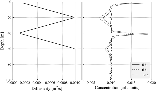
Figure 3: Concentration of initially well-mixed neutrally buoyant tracers, simulated with the naïve scheme (Eq. (44)), shown after different times. The number of particles was $N_{p}=$1\,000\,000$$, the timestep was $\Delta t=$300\text{\,}\mathrm{s}$$, and concentration is calculated by bin count in 100 bins of width $1\text{\,}\mathrm{m}$ each.

In the case of constant diffusivity, $K$, the random walk given by Eq. (38) simplifies to

$$\mathrm{d}z=v_{b}\,\mathrm{d}t+\sqrt{2K}\,\mathrm{d}W(t).$$ (43)

or discretised with Euler-Maruyama

$$z_{n+1}=z_{n}+v_{b}\Delta t+\sqrt{2K}\Delta W_{n}.$$ (44)

However, if $K$ is a function of position, Eq. (43) is not consistent with the advection-diffusion equation, and gives unphysical results where a net transport away from regions of high diffusivity is seen (Hunter et al., 1993; Holloway, 1994; Visser, 1997). The difference between the two schemes is the term $K^{\prime}(z)\Delta t$ in Eq. (38), which is known as the pseudovelocity term (Lynch et al., 2014, p. 125).

In oil spill modelling, it seems fairly common to use the random walk scheme described by Eq. (44), even in combination with spatially variable diffusivity. In, e.g., the plankton modelling community, the importance of using a consistent random walk appears to have been well known for two decades, with a particularly clear account of this issue being that of Visser (1997). In what follows, we will use the terminology of Visser, and refer to Eq. (44) as the naïve random walk.

An investigation of this issue in the context of oil spill modelling is presented in Nordam et al. (2019b), where it is found that use of the naïve random walk scheme may lead to both over- and underprediction of the amount of surface oil, compared to the consistent random walk scheme (Eq. (38)). The difference depends on the nature of the diffusivity profile, as well as the relevant droplet size distribution.

An example is shown in Fig. 3, where initially evenly distributed neutrally buoyant tracers have been modelled with the naïve scheme (Eq. (44)). We observe that the initially constant concentration profile breaks down, and the tracers start to accumulate in the regions of low diffusivity. While the example here uses neutrally buoyant particles, it is clear that this effect can lead to errors in modelling, e.g., the surfacing of small oil droplets.

7.2 Step-function diffusivity

Due to the difficulty of obtaining good data on the vertical diffusivity in the water column, simple schemes are sometimes used. For example, a step-function diffusivity profile may represent the well-known fact that diffusivity tends to be higher in the mixed layer, and lower below the pycnocline. An example of such a step-function profile used in oil spill modelling is found, e.g., in De Dominicis et al. (2016, Section 6.3):

$$K(z)=\left\{\begin{array}[]{lcc}${10}^{-2}\text{\,}{\mathrm{m}}^{2}\text{\,}{\mathrm{s}}^{-1}$&\mathrm{if}&z<$30\text{\,}\mathrm{m}$\\ ${10}^{-4}\text{\,}{\mathrm{m}}^{2}\text{\,}{\mathrm{s}}^{-1}$&\mathrm{otherwise}&\\ \end{array}\right.,$$ (47)

where depth is positive downwards. The diffusivity profile is illustrated in the left panel of Fig. 4.

It is clear that with this diffusivity profile, the Visser timestep criterion (Eq. (41)) can never be satisfied, and thus we cannot expect the well-mixed condition to be satisfied, regardless of the timestep. The problem can be understood intuitively by realising that particles that are in the high-diffusivity region, but close to the transition depth to low diffusivity, have a good probability to make a relatively large jump into the region of low diffusivity. Once there, however, it would take this particle a large number of steps to return to the region of high diffusivity. The net result is that the particles tend to accumulate in the region of low diffusivity, in violation of the WMC.

The results of a numerical test of the WMC are shown in the right panel of Fig. 4. Neutrally buoyant particles have been initially evenly distributed across the water column, down to a depth of $H=$100\text{\,}\mathrm{m}$$. A reflecting boundary condition has been used at the surface ($z=0$), and at the bottom ($z=H$). Concentration profiles are shown for different times, and it is clear that the particle count in the high-diffusivity region is depleted, for the reason described above. As described in the discussion of the WMC in Section 5.5, the correct solution to the diffusion equation in this case is that the concentration should remain constant.

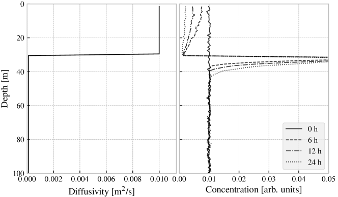
Figure 4: Concentration of initially well-mixed neutrally buoyant tracers, shown after different times. The number of particles wa $N_{p}=$10\,000\,000$$, the timestep was $\Delta t=$600\text{\,}\mathrm{s}$$, and concentration is calculated by bin count in 100 bins of width $1\text{\,}\mathrm{m}$ each.

While this example uses neutrally buoyant tracer particles, it is clear that this behaviour would also be a problem in an oil spill simulation. The effect of using this diffusivity profile is a net downwards displacement of particles, which leads to reduced surfacing rates in an oil spill model, particularly for small droplets with slow rise speeds.

We note that with this diffusivity profile, we have $K^{\prime}(z)=0$ everywhere, except at $z=$30\text{\,}\mathrm{m}$$, where the derivative of $K$ is a Dirac delta-function. Hence, the naïve random walk (Eq. (44)) and the corrected random walk (Eq. (38)) are identical in this case, except in a single point, and the inclusion of the pseudovelocity term does not compensate for the spurious downwards drift caused by the diffusivity profile.

We will now describe two approaches to avoid this problem. The first can be said to be a “workaround”, that modifies the diffusivity function to make it into a smooth approximation of a step function, while the second approach uses a different numerical scheme to solve the SDE for diffusion.

The “workaround” to simulating this problem would be to replace the step function diffusivity with a smooth sigmoid function with the same asymptotic values as the step function. In particular, the step function

$$K(z)=\left\{\begin{array}[]{lcc}K_{0}&\mathrm{if}&z<z_{0}\\ K_{1}&\mathrm{otherwise}\end{array}\right.,$$ (50)

can be approximated as

$$K(z)=K_{0}+\frac{K_{1}-K_{0}}{1+\mathrm{e}^{-a(z-z_{0})}},$$ (51)

where the value of the parameter $a$ determines the sharpness of the transition. By using a diffusivity profile given by Eq. (51), with large values of $a$, true step function diffusivity can be approximated arbitrarily well. If this is done in combination with a timestep that satisfies the Visser criterion (Eq. (41)), one can make sure the WMC is satisfied. For the sigmoid diffusivity profile given by Eq. (51), the Visser timestep criterion becomes

$$\Delta t\ll\frac{\sqrt{3}}{18}\cdot\left|\frac{1}{a^{2}(K_{0}-K_{1})}\right|.$$ (52)

As mentioned in Section 6.2, the timestep should be kept at least an order of magnitude below this limit. This may make the timestep impractically short if a large value of $a$ is chosen.

Another approach, which may be more efficient numerically, is to use the step-function diffusivity directly, but with a different numerical scheme for solving the SDE (Eq. (38)). Spivakovskaya et al. (2007a) describe an alternative to the Euler-Maruyama scheme, which they call the backward Itô scheme. In this scheme, the position, $z_{n+1}$, of a particle at time $t_{n+1}$ is given from its position $z_{n}$, at time $t_{n}$, by

$$\tilde{z}_{n} =z_{n}+\sqrt{2K(z_{n})}\Delta W_{n},$$ (53a)

$$z_{n+1} =z_{n}+v_{b}\,\Delta t+\sqrt{2K(\tilde{z}_{n})}\Delta W_{n},$$ (53b)

where $\Delta W_{n}$ is the same realisation of a Gaussian random variable with zero mean and variance $\langle\Delta W^{2}_{n}\rangle=\Delta t$ in both Eqs. (53a) and (53b). Hence, the net effect is to make a “trial step”, to a position $\tilde{z}_{n}$, and then use the diffusivity at that point, $K(\tilde{z}_{n})$, in the real step. With the backward Itô scheme, the WMC is satisfied for a step function profile. However, the backward Itô scheme does not work as well as Euler-Maruyama for, e.g., continuous, piecewise linear diffusivity functions. Experimentation is encouraged, to verify that a chosen combination of diffusivity profile, numerical scheme, and timestep satisfies the WMC to acceptable accuracy.

7.3 Linearly interpolated diffusivity

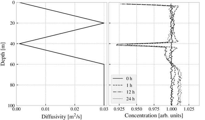
Figure 5: Concentration of initially well-mixed passive tracers, shown after different times. The number of particles was $N_{p}=$1\,000\,000$$, the timestep was $\Delta t=$300\text{\,}\mathrm{s}$$, and concentration is calculated by bin count in 100 bins of width $1\text{\,}\mathrm{m}$ each.

Many ocean models provide eddy diffusivity as output, along with with current, temperature, salinity, etc. If diffusivity is available, it can be used to drive the random walk, but care should be taken in the interpolation of the data. In particular, it is clear that the Visser timestep condition (Eq. (41)) can never be met if linear interpolation is used, as this will give a diffusivity profile that has piecewise constant first derivative, and hence a delta-function second derivative at each node in the interpolation.

As an example, we have carried out a test of the WMC for a piecewise linear diffusivity profile, as shown in the left panel of Fig. 5. While this profile is of course somewhat artificial, it has some realistic features, in that the diffusivity goes down towards the surface, and has a minimum at some value representing the pycnocline (see, e.g., Gräwe et al. (2012) for a thorough discussion of the problem of a sharp pycnocline). A passive tracer represented by $N_{p}=$1\,000\,000$$ particles was initially evenly distributed throughout the water column, down to a depth of $100\text{\,}\mathrm{m}$. Reflecting boundaries were used at the bottom and surface.

In the right panel of Fig. 5, concentration profiles are shown for different time points. The results clearly indicate that there are deviations from constant concentration at the minima of the diffusivity profile, as well as below 60 m depth, where the diffusivity is constant. The degree to which this happens depends on the timestep, as well as the diffusivity profile, and a sufficiently short timestep will in practical applications remove the problem. Nevertheless, this demonstrates that unexpected things may happen if one uses linear interpolation of input data without checking that the WMC is satisfied.

7.4 Chemically dispersed oil in the mixed layer

The final case is included as an example of a situation where a one-dimensional oil spill model may be of practical use. We consider an idealised situation where oil has been treated with surface dispersants, and dispersed into the water column by means of mechanical energy, either through waves, prop wash, water jetting or other means. The question is then, for a given droplet size, how long may one expect the oil to remain submerged. If the oil stays submerged for a long time, the dispersant operation may be said to have been successful.

In this idealised case, we will consider a single droplet size, and a sigmoid diffusivity profile giving a high diffusivity in the mixed layer, and a low diffusivity below the pycnocline (see Section 7.2). In particular we choose to use a diffusivity profile given by Eq. (51), with parameters $K_{0}=$1\text{\times}{10}^{-4}\text{\,}{\mathrm{m}}^{2}\text{/}\mathrm{s}$$, $K_{1}=$1\text{\times}{10}^{-2}\text{\,}{\mathrm{m}}^{2}\text{/}\mathrm{s}$$, $z_{0}=$20\text{\,}\mathrm{m}$$, and $a=$2\text{\,}{\mathrm{m}}^{-1}$$. The diffusivity profile is shown in the left panel of Fig. 6.

We consider two droplet sizes, $500\text{\,}\mathrm{\SIUnitSymbolMicro m}$, and $50\text{\,}\mathrm{\SIUnitSymbolMicro m}$. Assuming an oil density of $0.95\text{\,}\mathrm{kg}\text{/}\mathrm{L}$, and using Eq. (20) to calculate the rise speed, we get respectively $v_{b}=$5.4\text{\,}\mathrm{mm}\text{/}\mathrm{s}$$, and $v_{b}=$0.072\text{\,}\mathrm{mm}\text{/}\mathrm{s}$$.

Before presenting simulation results, we will try to reason about what might be expected to happen. A useful quantity to consider here is the Péclet number,

$$\mathrm{Pe}=\frac{vH}{K},$$ (54)

which gives the ratio between advective transport, and diffusive transport. Note that in our case, $v$ is the rise speed of the droplets, $H$ is the thickness of the mixed layer, and $K$ is the (average) diffusivity in the mixed layer. If $\mathrm{Pe}\gg 1$, the transport is advection-dominated (advection here refers to the rise speed of the droplets), and if $\mathrm{Pe}\ll 1$, the transport is diffusion-dominated. With the parameters described above, we get $\mathrm{Pe}\approx 11$ for the large droplets, and $\mathrm{Pe}\approx 0.15$ for the small droplets.

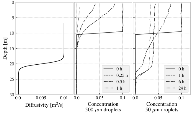
Figure 6: Left panel: Diffusivity as a function depth. Middle panel: Oil concentration, as a function of depth, for a droplet diameter of $500\text{\,}\mathrm{\SIUnitSymbolMicro m}$. Right panel: The same, for a droplet diameter of $50\text{\,}\mathrm{\SIUnitSymbolMicro m}$.

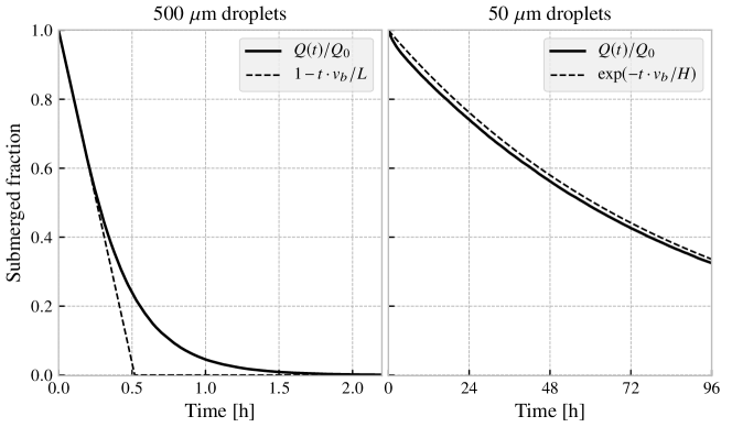
Figure 7: Left panel: Submerged fraction of oil, as a function of time, for a droplet diameter of $500\text{\,}\mathrm{\SIUnitSymbolMicro m}$. The idealised time development given by Eq. (55) is shown as a dashed line. Right panel: The same, for a droplet diameter of $50\text{\,}\mathrm{\SIUnitSymbolMicro m}$. The idealised time development given by Eq. (56) is shown as a dashed line.

Based on these considerations, we can begin to reason about the outcome of the dispersant operation, for the two droplet sizes we chose to look at. For the larger droplets, the vertical transport will be dominated by the rise speed. In the limit of zero diffusivity, the droplets will simply rise to the surface at their terminal velocity, $v_{b}$. If we assume an initial amount $Q_{0}$ of submerged oil, evenly distributed down to a depth $L$, then the amount of oil that remains submerged at time $t$ is simply given by

$$Q(t)=Q_{0}(1-t\frac{v_{b}}{L}),\;\;\;\;0<t<L/v_{b}.$$ (55)

When $t=L/v_{b}$, all the oil droplets have had time to reach the surface, and there is no submerged oil remaining. While the diffusivity will never be zero in a real case, we will see later that Eq. (55) provides a reasonable approximation if $\mathrm{Pe}\gg 1$.

For the small droplets transport is diffusion-dominated. Hence, they will be evenly distributed throughout the mixed layer, even if they were only initially entrained a short distance. Furthermore, the diffusivity in the mixed layer is sufficient to keep the remaining submerged droplets evenly distributed, even as the surfacing begins. We conclude that the fraction of submerged droplets that will surface during an interval $\Delta t$, is given by $v_{b}\Delta t/H$, where $H$ is the thickness of the mixed layer. When a constant fraction resurfaces during an interval, we have a first-order decay process. If the initial amount of submerged oil is $Q_{0}$, then the remaining submerged oil is given by:

$$Q(t)=Q_{0}\mathrm{e}^{-t/\tau},\;\;\;\;\tau=H/v_{b}.$$ (56)

Thus, we find that in addition to the difference in rise speed, there is also another difference that is relevant between advection-dominated transport (large droplets) and diffusion-dominated transport (small droplets), and that is the length scale. For large droplets, the entrainment depth is important, while for small droplets, the thickness of the mixed layer is important.

We will now look at some numerical simulation results. For both droplet sizes, we assume that the oil is initially evenly distributed down to a depth of $L=$10\text{\,}\mathrm{m}$$. We run simulations using $N_{p}=$100\,000$$ particles. For the diffusivity profile described above, the Visser timestep limit (Eq. (41)) gives $\Delta t\ll$42\text{\,}\mathrm{s}$$, and hence we choose $\Delta t=$2\text{\,}\mathrm{s}$$.

In Fig. 6, the concentration of oil droplets is shown as a function of depth, for different times. We observe that the large droplets rise quickly to the surface, and are not mixed any deeper than the initial depth of $L=$10\text{\,}\mathrm{m}$$. For the small droplets, we observe that they fairly quickly mix down to the pycnocline, and that the concentration thereafter remains approximately constant with depth throughout the mixed layer.

Figure 7 shows the remaining fraction of submerged oil as a function of time. Additionally, the idealised time developments given by Eqs. (55) and (56) are shown as a dashed lines.

The purpose of this example is to illustrate some special cases that may help provide some simple guidelines to reason about the outcome of a surface dispersant operation. In particular, we observe that if we assume $\mathrm{Pe}\gg 1$, then the time for the oil to surface is largely governed by the entrainment depth and the rise velocity. On the other hand, if $\mathrm{Pe}\ll 1$, then the time development is determined by the depth of the pycnocline and the rise velocity. The diffusivity does not appear in either case, other than in the estimation of $\mathrm{Pe}$.

Finally, we note that it is of course not realistic to consider the entrainment and surfacing of oil as a purely one-dimensional problem over a period of several days, as in the right panel of Figs. 6 and 7. During this time, the oil will certainly be subject to horizontal advection and diffusion. This is of course precisely the goal of a surface dispersant operation, and such an operation will probably be said to be successful if the majority of the oil may be expected to remain submerged for several days.

8 Example cases

From the discussion in the preceding sections, it should be clear that the vertical movement of oil in the water column is an interplay between different effects. Entrainment moves oil from the surface, and into the water column. Buoyancy transports oil upwards, and eventually to the surface, at a rate that is dependent on the droplet size distribution (which in turn depends on the conditions during entrainment).

Turbulent mixing tends to distribute the oil in the vertical. While this diffusion process does not itself have a preferred direction, the net effect can still be to move the center of mass of a concentration profile either up or down, due to the reflecting boundary at the surface, vertical variation in diffusivity, and depending on initial conditions.

In breaking wave conditions there will always be some entrainment of surface oil. Hence, some fraction of the oil will be submerged at any time, and some fraction will remain at the surface. The fraction at the surface will depend on wave conditions, vertical diffusivity in the subsurface, and the state of the oil (since droplet size distribution depends, among other things, on the viscosity of the oil). The surface fraction will change with time even if the wave conditions remain constant, as the oil weathers, and since the smaller droplets may remain submerged for a very long time.

It is clear that even though oil is typically buoyant, it is quite possible for the majority of the oil in a surface spill to be transported in the subsurface, in a state of dynamic equilibrium between entrainment and resurfacing. As discussed in the introduction, the vertical distribution of oil may have significant impact on horizontal transport, due to current shear effects. The aim of this section is to provide some examples of real oil spill scenarios where the vertical distribution of oil is of particular importance to the horizontal transport.

8.1 The 1993 Braer oil spill

On January 5, 1993, MV Braer ran aground within 100 meters of the coast of Shetland (Reed et al., 1999) during a storm. It was carrying $85\,000$ tonnes of Gullfaks crude oil, which was released into the ocean over a period of several days (Spaulding et al., 1994). During the event, model forecasts were made available, but failed to accurately predict the movement of the oil (Turrell, 1994, 1995). Later, several hindcast modelling studies were made (see, e.g., Spaulding et al. (1994); Turrell (1994); Proctor et al. (1994)).

While the wind was mainly flowing towards the north-east, much of the oil moved towards the south, with oil found in the sediments up to $100\text{\,}\mathrm{km}$ to the south of the spill site (Proctor et al., 1994). One explanation would be that the relatively light Gullfaks crude dispersed as small droplets in the strong winds present during the spill, causing a large fraction of the spilled oil to be transported towards the south by the subsurface currents. An additional relevant mechanism is that of oil-mineral aggregation (which has not been discussed in this chapter), which may cause oil to sink when associated with high density mineral particles.

8.2 The 2011 Golden Trader oil spill

On September 10, the bulk carrier MV Golden Trader collided with a fishing vessel off the north-west coast of Denmark. There were no casualties, but some bunker fuel was spilled from MV Golden Trader. The amount was later estimated at 150 tonnes. During the first two days after the spill, approximately 50 tonnes of oil were collected by Danish response vessels. After this, the wind picked up, and no further observations of oil were reported until September 15, when oil reached the Swedish shore. On September 16, it became clear that a significant amount of oil (estimated amount 25–30 tonnes) had beached (Transport Malta, 2012).

The distance from the release point to the site of the beaching is more than $250\text{\,}\mathrm{km}$. Only approximately $15\text{\,}\mathrm{km}$ of the shoreline was heavily oiled (ITOPF, 2011). Combined with the fact that beaching appears to have occurred over a period of half a day or more, this indicates that the slick may have been elongated in the wind direction, and relatively narrow in the cross-wind direction, as discussed by, e.g., Johansen (1982) and Elliott (1986).

To the best of our knowledge, no detailed hindcast of this incident has been published. Such a hindcast would however be an interesting exercise. It seems likely that a number of model processes will impact the arrival time of the oil and the site of the beaching, including droplet size distribution, vertical mixing, and possibly Stokes’ drift (Broström et al., 2014).

9 Advanced topics and further reading

Historically, the mathematical and technical details of Lagrangian particle schemes have received limited attention in papers on oil spill modelling (see, e.g., Nordam et al. (2019b) and references therein). A challenge is that the mathematical literature on Stochastic differential equations is often very technical, and not very accessible to non-specialists. However, there exists a large body of work on the modelling of plankton, fish eggs, sediment particles, atmospheric dispersion, etc., where these schemes are treated more rigorously that what is commonly seen in the oil spill modelling literature. Much of this work is formulated in terms of familiar concepts from applied oceanography, and may be more or less directly applied to the transport part of oil spill modelling.

In this section, we discuss some advanced topics, and recommend some further reading for those who are interested in the details of these topics.

9.1 Higher-order SDE solvers

Earlier, we used the Euler-Maruyama scheme to discretise Eq. (38), obtaining the following iterative scheme for particle positions:

$$z_{n+1}=z_{n}+\big{(}w+K^{\prime}(z_{n})\big{)}\Delta t+\sqrt{2K(z_{n})}\Delta W_{n}.$$

However, just like the Euler scheme is the simplest, and least accurate, ODE solver, so the Euler-Maruyama scheme is the simplest and least accurate SDE solver. Switching to higher-order schemes should in principle give improved accuracy at the same timestep, or reduce computational effort by allowing a longer timestep to be used.

For SDE schemes, two types of convergence exist, weak and strong. Convergence in the weak sense means that for a large number of particles, the distribution of particles will converge towards the true distribution (which may or may not be known) as the timestep goes to zero. Technically, weak convergence is expressed in the following way: If, for a numerical SDE scheme, and for sufficiently short timesteps $\Delta t$, there exists a constant $C$, such that

$$|\langle f(z_{N})\rangle-\langle f(z(t_{N}))\rangle|<C\Delta t^{\gamma},$$ (57)

then the scheme is said to have order of convergence $\gamma$ in the weak sense. Here, $z_{N}$ is the numerical approximation at time $t_{N}$, and $z(t_{N})$ is the true solution at the same time, and the angle brackets indicate ensemble average over many independent particles. The functions $f$ are continuous functions that have polynomial growth, and are at least $2(\gamma+1)$ times differentiable. Since this class of functions include all the integer powers of $z$, it follows that the moments of the distribution converge if the scheme converges in the weak sense. As any distribution is uniquely defined by its moments, this means that the modelled distribution converges to the true distribution.

Convergence in the strong sense is also called pathwise convergence. If, for a numerical SDE scheme, and for sufficiently short $\Delta t$, there exists a constant $C$, such that

$$\langle|z_{N}-z(t_{N})|\rangle<C\Delta t^{\gamma},$$ (58)

then the scheme is said to have order of convergence $\gamma$ in the strong sense.

The Euler-Maruyama scheme has orders of convergence $1/2$ in the strong sense, and $1$ in the weak sense. Higher-order schemes exist, but the complexity of the schemes grows fast as the order increases. An example of a higher order scheme is the 1st-order Milstein scheme, which has order of convergence 1, in both the strong and the weak sense (see, e.g., Kloeden and Platen (1992, p. 345)). Applied to our SDE for advection-diffusion problems (Eq. (38)), the 1st-order Milstein scheme yields

$$z_{n+1}=z_{n}+\big{(}w+K^{\prime}(z_{n})\big{)}\Delta t+\sqrt{2K(z_{n})}\Delta W_{n}+\frac{1}{2}K^{\prime}(z_{n})(\Delta t-\Delta W_{n}^{2}).$$ (59)

Gräwe et al. (2012) argue that in some cases, the Euler-Maruyama scheme is simply inadequate, even with very short timesteps. The example they give is that of a strong, sharp pycnocline where the diffusivity will drop almost to zero at the steepest point of the density gradient. In such a case, passive tracers should cross the pycnocline very slowly, a behaviour that is modelled far more accurately by the 1st-order Milstein scheme, due to its higher order of convergence in the strong sense.

For a clear and readable presentation of a range of numerical SDE schemes, with a view to marine particle tracking applications, the interested reader is referred to Gräwe (2011); Gräwe et al. (2012). Note however that some of the schemes have been found to contain small mistakes, hence it is also advisable to consult other sources prior to implementation, for example the classic work by Kloeden and Platen (1992).

9.2 Autocorrelated velocity or acceleration

Implementing a random walk scheme that makes random displacements at each timestep, with no correlation in time, makes the implicit assumption that a moving particle can instantly change its velocity. This may seem unreasonable. Furthermore, when very short timesteps are used we find that particle speed becomes arbitrarily large, since the average step-length is proportional to $\sqrt{2K\Delta t}$, and we have

$$\lim_{\Delta t\to 0}\frac{\sqrt{2K\Delta t}}{\Delta t}=\infty$$ (60)

for any positive $K$. Note, however, that while these points sound unreasonable from a physical point of view, there is no problem in using the random walk scheme with short timesteps. Eq. (38) was derived to be consistent with the advection-diffusion equation, and in the limit $\Delta t\to 0$, $N_{p}\to\infty$, the distribution of particles will converge to correct distribution, almost surely (provided $K(z)$ and $K^{\prime}(z)$ are sufficiently smooth functions).

In fact, the “infinite speed” of the particle is a feature which is built into the model from the start: The Wiener process, $W(t)$, whose increments appear in Eq. (38), has infinite total variation on any interval of non-zero length (Brzeźniak and Zastawniak, 1999, pp. 157–158). The apparent problem stems only from trying to extract a physically meaningful “speed” from a model that does not contain the speed of the particle as a variable.

Nevertheless, it might in some cases be desirable to have a more physically realistic random walk model. Recall that what we have been calling diffusivity, is in reality a parameterisation of mixing due to turbulence. If we consider a neutral tracer in a field of turbulent eddies, it is clear that the velocity at one instant will be at least somewhat correlated to the velocity a short time later. This behaviour can also be captured in numerical modelling.

Lynch et al. (2014) describe a hierarchy of random walk models with different degrees of autocorrelation. The standard random walk that we have been considering so far is called AR0 in this hierarchy, as it has no autocorrelation in the displacement at each step. (Note that the position of a particle does of course have autocorrelation, as the position at time $t_{n}$ depends on the position at time $t_{n-1}$.)

The next level of the hierarchy is called AR1, where the displacement at each step is related to the displacement at the previous step. In this scheme, there is autocorrelation not only in the position of a particle, but also in its velocity. This is in a way a more realistic model, as in reality, the movement of a particle from one instant to the next is correlated, with the de-correlation time being dependent on the turbulent fluctuations.

The original Langevin equation was formulated to describe Brownian motion, i.e., the apparently random motion of small particles in fluids, caused by collisions with the molecules of the fluid (Langevin, 1908; Lemons and Gythiel, 1997), and reads

$$m\frac{\mathrm{d}^{2}x}{\mathrm{d}t^{2}}=-6\pi\mu a\frac{\mathrm{d}x}{\mathrm{d}t}+X.$$ (61)

Here, $m$ is the mass of the particle, $-6\pi\mu a\frac{\mathrm{d}x}{\mathrm{d}t}$ is the drag force from the bulk fluid, and $X$ is a random force representing the collisions of molecules. Hence, this is simply Newton’s second law, with a random component in the force.

Along the same lines, Lynch et al. (2014) write down a general equation for an AR1 scheme as,

$$\frac{\mathrm{d}^{2}z}{\mathrm{d}t^{2}}+\frac{1}{\tau}\frac{\mathrm{d}z}{\mathrm{d}t}=\eta,$$ (62)

where $\eta$ is some random process acting as a forcing, and $\tau$ is a timescale for decay of the velocity if no forcing is applied. Written as a pair of coupled first-order SDEs in standard notation, this becomes

$$\begin{aligned} \mathrm{d}v&=-v\frac{1}{\tau}\,\mathrm{d}t+\eta\,\mathrm{d}W_{t},\\ \mathrm{d}z&=v\,\mathrm{d}t.\end{aligned}$$ (63)

In this model, there is a time-correlation in the movement of the particle, since the velocity will only change by a small amount between timesteps. This is also called a “random flight”. It should be noted that an AR1 scheme is fundamentally different from an AR0 scheme, in that it is not consistent with the diffusion equation. And that is of course the argument for using this schemes in the first place, since what we are trying to model is turbulent mixing, and not pure diffusion.

AR1 schemes have a long history of usage in dispersion models for the atmosphere (Thomson, 1987). However, comparisons between this and the AR0 scheme have shown small differences in the far-field (Wilson and Yee, 2007). This implies that differences in the results of an oil spill simulation are unlikely to be substantial.

A review by Spaulding (2017) mentions regarding an AR1 scheme that “[u]se of this higher order model is possible if one has accurate estimates of the currents and dispersion”, but does not elaborate further. A recent paper by Cui et al. (2018) solves the so-called Maxey-Riley equation, describing the inertia and drag forces on individual oil droplets due to turbulent motion of the surrounding waters, and compare the results to a regular random walk scheme. However, this work considers only small spatial scales underneath breaking waves, and the effects on larger scales are not investigated.

In conclusion, AR1 (or even higher order) schemes do not appear to be commonly used in oil spill modelling. In addition to the increased mathematical and numerical complexity, a practical problem in using an AR1 scheme is that one can no longer use the eddy diffusivity directly, but must instead obtain estimates of the parameters $\tau$ and $\eta$ in Eq. (62). The interested reader is referred to Lynch et al. (2014), and references therein, as well as the literature on atmospheric dispersion (see, e.g., Thomson (1987), Wilson and Flesch (1993)).

9.3 Reconstructing a concentration field from particles

As discussed in Section 6, our random walk scheme is in some sense equivalent to the advection-diffusion equation. The link is that each particle, at time $t_{n}$, represents a sample from the distribution at that time, where the distribution develops according to the advection-diffusion equation. If we want to (approximately) reconstruct the distribution from the particles, there are several different approaches, and which is most suitable may depend on the application. We discuss these in one dimension in this section, but generalisation to several dimensions is natural.

The simplest approach is the so-called box count or bin count, which consists of dividing the region of interest into discrete bins, and counting the number of particles in each bin. The concentration in each bin is then proportional to that number, weighted by the particle mass if each particles represents a different mass. This is exactly the same as a weighted histogram of particle positions.

We let our cells have constant size $\Delta z$, and define cell $i$ by $(i-1)\Delta z\leq z<i\Delta z$. Furthermore, let particle $j$ have position $z_{j}$ and represent a mass $m_{j}$. Then the concentration, $C_{i}$, in cell $i$, is given by

$$C_{i}=\frac{1}{\Delta z}\sum m_{j}\textrm{ for all }j\textrm{ such that }(i-1)\Delta z\leq z_{j}<i\Delta z,$$ (64)

where $N_{p}$ is the total number of particles. A natural question to ask is then how the error in the concentration scales with the number of particles and the cell size.

We recall that the particle positions are essentially random samples, and two simulations will in general give somewhat different concentration fields due to this randomness. The difference between the true distribution (which is usually unknown), and the reconstructed distribution based on $N_{p}$ samples, is called the sampling error. One may see from the Central Limit Theorem (Billingsley, 1979, p. 308), that the sampling error scales as $1/\sqrt{N_{p}}$ where $N_{p}$ is the number of independent samples. This means that increasing the number of particles by a factor of 10 will only reduce the error by a factor of $\sqrt{10}$.

Regarding cell size, there is a choice to be made between resolution and sampling error. In the case where the entire domain is covered by just one cell, then all the particles will be inside that cell, which is of course correct, but also a useless result. On the other hand, if there are so many cells that most cells have either 0 of 1 particles, then the result is completely dominated by random sampling noise. The challenge is to use enough cells to resolve those changes in concentration that are of interest, and enough particles to give a reasonably smooth result.

Box counting often leads to very noisy concentration fields. In particular, if one is interested in the most dilute concentrations, the results are guaranteed to be noisy, because the most dilute concentrations are by definition represented by only a small number of particles. However, even the higher concentrations may be noisy. A common way to tackle this problem is to use a kernel, where each particle is not treated as a point, but as a distribution with a finite extent. In statistics, this is called Kernel Density Estimation (KDE). For further details, see, e.g., Silverman (1986).

The kernel function, $\kappa(z)$ must be a positive function, with the property

$$\int_{-\infty}^{\infty}\kappa(z)\,\mathrm{d}z=1.$$ (65)

Usually, $\kappa(z)$ is also symmetric, and with a maximum at $z=0$. Then the concentration field, $C(z)$, is given by

$$C(z)=\frac{1}{N_{p}}\sum_{j=0}^{N_{p}}\frac{m_{j}}{\lambda j}\,\kappa\left(\frac{z-z_{j}}{\lambda_{j}}\right),$$ (66)

where $z_{j}$ and $m_{j}$ are as before the position and mass of particle $j$, and $\lambda_{j}$ is called the bandwidth of particle $j$. For a given kernel function, increasing the bandwidth will widen the kernel, and give a smoother (but less detailed) concentration field. Hence, the choice of both kernel and bandwidth becomes important, with the bandwidth typically more important than the kernel (for standard choices of kernel function).

An example comparing box count and KDE is shown in Fig. 8. Here, 10 random particle positions were drawn from a Gaussian distribution with mean 0.5, and standard deviation 0.1. In the left panel, a box count on 10 cells of length $\Delta z=0.1$ was used. In the right panel, KDE was used, with a Gaussian kernel (unit variance), and a constant bandwidth of $\lambda=0.1$. It is clear that the density reconstructed by KDE gives a much smoother result, and a better approximation of the underlying distribution.

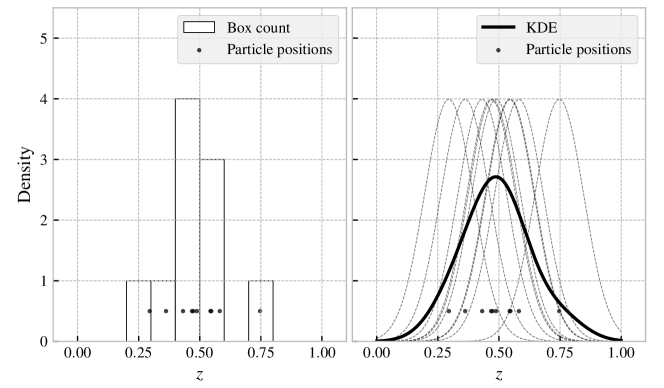
Figure 8: Probability density reconstruction based on $N_{p}=10$ random particle positions, drawn from a normal distribution. In the left panel, box count (histogram) is used. In the right panel, KDE is used with a Gaussian kernel (unit variance) and a bandwidth of $\lambda=0.1$. The bandwidth-scaled kernel of each individual particle is shown as a thin, dashed line. In both cases, the particle positions were the same.

For further reading on this topic, see e.g., Lynch et al. (2014, Chapter 8).

10 Summary

The aim of this chapter has been to introduce the reader to most processes that are relevant for modelling of the vertical distribution of oil spilled at sea, with the exception of near-field plume modelling. It is our hope that the reader will find themselves able to understand, and indeed implement, numerical models for the relevant vertical transport processes. We have also tried to give references to further reading, indicate what some uncertainties are, and point out some examples of problems that require more research.

An eternal problem of oil spill modelling is that of input data. We know that there are always large uncertainties in meteorological input, perhaps most importantly in the currents. Likewise, modelling vertical eddy diffusivity is a research field in itself, and it may be difficult to know what diffusivity profiles to use as input to the oil spill modelling.

It is worth remembering that oil spill modelling is, to some degree, an exercise in pragmatism. This is especially true for operational modelling in support of oil spill response, where time is of the essence, and good data might be hard to obtain. For model development in general, it is also worth considering where the largest uncertainties lie, and putting the effort there.

In general, we encourage experimentation and testing, to make sure models satisfy those exact solutions that are known to exist, such as the WMC. We would also suggest that some attention is paid to numerical schemes, even though these are usually not the source of the largest errors. Using bad numerical schemes can lead to large and systematic errors, and can mask the improvements of model development in other areas.

We have also made a point of introducing, e.g., the Péclet number and the Richardson number, that can sometimes be used to characterise situations as either diffusion dominated, or advection dominated. It is easy to think that the job of an oil spill modeller is to run an oil spill model on a set of input data, but by taking a critical look at those data one can sometimes reason quite successfully about the expected outcome of a situation.

Finally, we would like to encourage our readers to stay curious, to experiment with models, to read papers from related research fields, and to contribute to the literature by publishing detailed descriptions of new modelling developments.

Appendix A Equivalence between Eulerian and Lagrangian pictures

The development of a concentration field under transport and mixing may be described by the Partial Differential Equation (PDE) known as the advection-diffusion equation. This is called an Eulerian approach, and is characterised by an equation that describes how the concentration at fixed locations changes in time. The same process may also be described by an ensemble of “particles” which experience directed motion due to advection, and random motion due to diffusion. This approach is called Lagrangian, and is characterised by an equation that describes how the position of a particle changes with time.

The link between the Eulerian and the Lagrangian picture is that the concentration field described in the Eulerian picture, if normalised, describes a probability distribution for where the Lagrangian particles will be found. Conversely, calculating the position of a Lagrangian particle is the same as drawing a sample from the probability distribution, and with a large number of samples, the distribution can be reconstructed approximately. We will here demonstrate how to obtain a random walk which is equivalent to the advection diffusion equation.

Consider a diffusion process described by the general Stochastic Differential Equation (SDE)

$$\mathrm{d}z=a(z,t)\,\mathrm{d}t+b(z,t)\,\mathrm{d}W(t),$$ (67)

where $a(z,t)$ and $b(z,t)$ are “moderately smooth functions” (Kloeden and Platen, 1992, p. 37), and $\mathrm{d}W(t)$ are the increments of a standard Wiener process (Kloeden and Platen, 1992, p. 40). Further conditions also apply, though these may be less important in practice. For details see, e.g., Gihman and Skorohod (1972, pp. 96–102).

For this diffusion process, the Fokker-Planck equation (also known as the Kolmogorov Forward equation) for evolution of the transition probability density, $p(z_{0},t_{0},z,t)$, from an initial position $z_{0}$ at time $t_{0}$, to a position $z$ at a later time $t$, is (Kloeden and Platen, 1992, p. 37):

$$\begin{aligned} \frac{\partial p(z_{0},t_{0},z,t)}{\partial t}&=\frac{1}{2}\frac{\partial^{2}}{\partial z^{2}}\Big{(}b^{2}(z,t)\,p(z_{0},t_{0},z,t)\Big{)}\\ &-\frac{\partial}{\partial z}\Big{(}a(z,t)\,p(z_{0},t_{0},z,t)\Big{)}.\end{aligned}$$ (68)

We observe that the Fokker-Planck equation is a PDE, and like the advection-diffusion equation, it describes the time-development of a distribution. For a particle initially at position $z_{0}$ at $t_{0}$, undergoing the random motion described by Eq. 67, the probability density function for the position, $z$, at a later time, $t$, may be obtained by the Fokker-Planck equation. If we consider instead a large ensemble of particles, all starting out at $z_{0}$ at $t_{0}$, then at a later time $t$, they will be distributed according to $p(z_{0},t_{0},z,t)$, with many particles in areas of high probability and few particles in areas of low probability.

This is equivalent to the evolution of a concentration field from an instantaneous point source, as described by the advection-diffusion equation. Hence, our goal is to obtain the SDE which has the advection-diffusion equation as its Fokker-Planck equation. Then we know that the distribution of an ensemble of particles will develop according to the advection-diffusion equation, and thus we can use the distribution of particles to approximately reconstruct the concentration field.

Going back to Eq. (68), we drop the arguments to $a$, $b$ and $p$ for brevity, and rewrite the equation a bit, and we get

$$\frac{\partial p}{\partial t} =\frac{1}{2}\frac{\partial}{\partial z}\left(b^{2}\frac{\partial p}{\partial z}\right)-\frac{\partial}{\partial z}\left[\left(a-\frac{1}{2}\frac{\partial b^{2}}{\partial z}\right)p\right].$$ (69)

We then compare Eq. (69) to the advection-diffusion equation, with advection $w(z,t)$ and diffusion $K(z,t)$:

$$\frac{\partial C}{\partial t}=\frac{\partial}{\partial z}\left(K\frac{\partial C}{\partial z}\right)-\frac{\partial}{\partial z}\left(wC\right).$$ (70)

By demanding that $C$ should be proportional to $p$ at all times, we find that each term in Eq. (69) must be equal to the corresponding term in Eq. (70). We thus obtain

$$K=\frac{b^{2}}{2}\; \Rightarrow\;b=\sqrt{2K}$$ (71a)

$$w=a-\frac{1}{2}\frac{\partial b^{2}}{\partial z}\; \Rightarrow\;a=w+\partial_{z}K$$ (71b)

Hence, the SDE whose probability density is described by the advection-diffusion equation is

$$\mathrm{d}z=(w+K^{\prime}(z))\,\mathrm{d}t+\sqrt{2K(z)}\,\mathrm{d}W,$$ (72)

where $K^{\prime}(z)=\partial_{z}K$.

Note that since both $a(z,t)$ and $b(z,t)$ in Eq. (67) must be continuous, we find that both $K(z)$ and $\partial_{z}K(z)$ must be continuous for the conditions mentioned above to be satisfied. Hence, the equivalence with the advection-diffusion does not hold for, e.g., step-function diffusivity, or piecewise linear diffusivity profiles with discontinuous first derivatives, such as a linearly interpolated profile.

References

-
Billingsley (1979)
Billingsley, P.
1979. Probability and measure. New York Chichester Brisbane Toronto: John Wiley & Sons. -
Booij et al. (1997)
Booij, N., L. Holthuijsen, and R. Ris
1997. The” swan” wave model for shallow water. In Proceedings of the 25th International Conference on Coastal Engineering, Orlando, Florida, 1996, Pp. 668–676. -
Bowden (1965)
Bowden, K.
1965. Horizontal mixing in the sea due to a shearing current. Journal of Fluid Mechanics, 21(1):83–95. -
Bowles et al. (1958)
Bowles, P., R. Burns, F. Hudswell, and
R. Whipple
1958. Sea disposal of low activity effluent. In Proceedings of the Second United Nations International Conference on the Peaceful Uses of Atomic Energy, Geneva, Switzerland, volume 18, Pp. 376–389. -
Bozzano and Dente (2001)
Bozzano, G. and M. Dente
2001. Shape and terminal velocity of single bubble motion: a novel approach. Computers & Chemical Engineering, 25(4):571 – 576. -
Brandvik et al. (2013)
Brandvik, P. J., Ø. Johansen, F. Leirvik, U. Farooq, and P. S.
Daling
2013. Droplet breakup in subsurface oil releases – part 1: Experimental study of droplet breakup and effectiveness of dispersant injection. Marine Pollution Bulletin, 73(1):319 – 326. -
Broström et al. (2014)
Broström, G., M. Drivdal, A. Carrasco, K. Christensen, and
J. Mattsson
2014. The golden trader oil spill; evaluation of operational oil spill models. In EGU General Assembly Conference Abstracts, volume 16. -
Brzeźniak and
Zastawniak (1999)
Brzeźniak, Z. and T. Zastawniak
1999. Basic stochastic processes. London: Springer-Verlag. -
Carslaw and Jaeger (1959)
Carslaw, H. S. and J. C. Jaeger
1959. Conduction of heat in solids. Oxford University Press (Clarendon), Oxford, UK. -
Carter (1982)
Carter, D.
1982. Prediction of wave height and period for a constant wind velocity using the jonswap results. Ocean Engineering, 9:17–33. -
Clift et al. (1978)
Clift, R., J. R. Grace, and M. E. Weber
1978. Bubbles, drops, and particles. New York: Academic Press. -
Craig and Banner (1994)
Craig, P. D. and M. L. Banner
1994. Modeling wave-enhanced turbulence in the ocean surface layer. Journal of Physical Oceanography, 24(12):2546–2559. -
Csanady (1973)
Csanady, G.
1973. Turbulent diffusion in the environment. Dordrecht, Holland: D. Reidel Publishing Company. -
Cui et al. (2018)
Cui, F., M. C. Boufadel, X. Geng, F. Gao, L. Zhao, T. King, and
K. Lee
2018. Oil droplets transport under a deep-water plunging breaker: Impact of droplet inertia. Journal of Geophysical Research: Oceans, 123(12):9082–9100. -
Davidson (2015)
Davidson, P. A.
2015. Turbulence: An introduction for scientists and engineers, 2nd edition. Oxford, UK: Oxford University Press. -
De Dominicis et al. (2016)
De Dominicis, M., D. Bruciaferri, R. Gerin, N. Pinardi, P. Poulain, P. Garreau,
G. Zodiatis, L. Perivoliotis, L. Fazioli, R. Sorgente, and
C. Manganiello
2016. A multi-model assessment of the impact of currents, waves and wind in modelling surface drifters and oil spill. Deep Sea Research Part II: Topical Studies in Oceanography, 133:21–38. -
Delnoij et al. (1997)
Delnoij, E., F. Lammers, J. Kuipers, and W. P. M. van
Swaaij
1997. Dynamic simulation of dispersed gas-liquid two-phase flow using a discrete bubble model. Chemical engineering science, 52(9):1429–1458. -