[type=editor, auid=000,bioid=1, prefix=, role=, orcid=0000-0002-6978-8663] \cormark[1]
Conceptualization, Methodology, Data curation, Writing - Original draft preparation
Conceptualization, Methodology, Data curation, Writing - Original draft preparation
Conceptualization, Methodology, Data curation, Writing - Original draft preparation
[cor1]Corresponding author
Effect of geometric parameters on the noise generated by rod-airfoil configuration
Abstract
This paper investigates the effect of the geometric parameters – rod diameter and the distance between the rod and the airfoil – on the noise generated by rod-airfoil configuration using experimental and numerical techniques. The numerical simulations are carried out using the low-dissipation up-wind scheme and the Delayed-Detached-Eddy Simulation (DDES) approach with Shear-Layer Adapted (SLA) sub-grid length scale (SGS) for a faster transition between RANS and LES. A dual-time stepping strategy, leading to second-order accuracy in space and time, is followed. The Ffowcs-Williams and Hawkings (FWH) technique is used to post-process the pressure fluctuations to predict the far field acoustics. A corresponding detailed experimental analysis, carried out using phased microphone array techniques in the aeroacoustic wind tunnel at the Brandenburg Technical University at Cottbus, is used for the validation of the numerical method. The key objective of the analysis is to examine the influence of the parameters of the configuration on the noise generation. The results show reasonable agreement with the experimental data in terms of far-field acoustics.
keywords:
rod-airfoil \sepbroadband noise \sepDDES \sepFW-H \sepmicrophone array1 Introduction
An airfoil subjected to a real flow emits noise that mainly consists of two components: the first is the leading edge (LE) noise, which results due to the interaction of the leading edge of the airfoil and the turbulent inflow, and the second one is the trailing edge noise, which results due the interaction of the airfoil boundary layer with the trailing edge. The former becomes an important broadband noise generating mechanism in terms of unsteady loading at reasonable angles of attack and highly perturbed flow [1]. As such it is observed in many practical applications like turbomachinery due to the interaction between the rotor wake and the leading edges of the downstream located stator blades [2, 3, 4]. To investigate the generation of such a phenomenon, a rod-airfoil test case has been continuously investigated due to the fact that its geometry contains some of the aerodynamic mechanisms found in turbomachinery applications, but remains computationally simple enough to allow parametric studies [5]. In such a configuration, a cylindrical rod is installed upstream of an airfoil, and when introduced in a flow field, the upstream rod generates a turbulent wake (a von Kármán vortex street, consisting of counter-rotating vortices resulting in a nearly constant Strouhal number , where is the shedding frequency, the rod diameter and the flow velocity), which then interacts with an airfoil downstream. This configuration has been studied by many researchers. [6] was the first to investigate this problem using unsteady RANS simulations. The simulations were two-dimensional and the three dimensional effects on noise were modelled using a statistical model coupled with the Ffowcs Williams and Hawkings (FW-H) equation [7] based on the Lighthill’s acoustic analogy. Boudet et al. [8] reported the first LES computations for this benchmark problem using a finite-volume, compressible LES on multi-block structured grids. Far-field noise was obtained by coupling the near-field data with a permeable FW-H solver. Jacob et al. [5] used the experimental acoustic results measured on a rod-airfoil setup for the verification of the numerical broadband noise calculations. Their work has become a standard against which other researchers have benchmarked their code capability and accuracy.
In order to be able to predict sound sources and in particular broadband sources directly, highly accurate transient computational fluid dynamics (CFD) solutions must be obtained. A variety of numerical approaches, including unsteady Reynolds averaged Navier-Stokes (URANS) [6, 5] and large eddy simulations (LES) [9, 10, 11, 12] have been used to study the rod-airfoil configuration. It should also be noted that the highly unstable phenomena resulting due to the impingement of the turbulent wake on the airfoil, the main source of radiation, are difficult for RANS to resolve. However, it is possible to simulate the flow around the rod-airfoil configuration with the direct numerical simulation (DNS) without any form of turbulence modelled artificially at the cost extraordinary CPU time. The computational effort of three-dimensional DNS scales with the Reynolds number , making the approach not viable for practical airfoil simulations. On the other hand, the computational cost and the available resolution of LES stands between RANS and DNS. LES resolves the large scales eddies (more than 80% of the turbulent kinetic energy should be resolved [13]), while the small scale (sub-grid scale (SGS)) are modelled. To address the small turbulent scales, LES requires higher grid resolution and corresponding smaller time-steps than RANS. This results in higher computational costs. Moreover, at rigid boundaries, LES does not respond well. An alternative to compromise the computational costs and the accuracy is the detached eddy simulation (DES). DES is a hybrid model that acts as RANS in the near-wall regions and LES in separate flow areas, integrating advantages of both approaches and being less demanding than the pure LES [14]. DES solutions should approach the quality of an LES prediction at optimised processor costs and are therefore a great choice for rod-airfoil simulations. The DES methodology used by Greschner et al. [15] suggests the efficiency and accuracy of the system for the estimation of the flow over blunt bodies. In a delayed detached eddy simulation (DDES) model, Zhou et al. [16] used the rod-airfoil configuration to optimise the NACA 0012 airfoil shape with regard to minimum turbulence-interaction noise. The recent work on the rod-airfoil configuration with DES and LES is summarised in Table 1.
| Name | Method | Mesh |
| Zhou et al. [16] | DDES | 3D Unstructured |
| Jiang et al. [12] | LES | 3D Structured |
| Agrawal and Sharma [11] | LES | 3D Unstructured |
| Giret et al. [10] | LES | 3D Unstructured |
| Galdeano et al. [17] | DES | 3D Unstructured |
| Berland et al. [9] | LES | 3D Structured |
| Greschner et al. [18] | DES | 3D Structured |
| Caraeni et al. [19] | DES | 3D Unstructured |
| Gerolymos and Vallet [20] | DES | 3D Structured |
| Greschner et al. [15] | DES | 3D Unstructured |
| Present study | DDES | 2D and 3D Unstructured |
The aforementioned studies were mostly conducted on one rod–airfoil configuration with fixed rod diameter and/or streamwise gap. In a prior experimental study, [21] examined the effect of the rod diameter and the streamwise gap on the broadband noise. The present work follows [21] by further investigating the effects of these two parameters on the radiated noise, especially the influence of the gap/diameter ratio. The main objectives of the present research are
-
1.
Investigation of the influence of geometric parameters (namely the rod diameter and the streamwise gap between rod and airfoil) at low Mach number flow speeds on the noise generation.
-
2.
Applying the compressible DDES approach to calculate the near-field CFD results and using the Ffowcs-Williams and Hawkings (FWH) approach to predict far-field noise.
This paper is organised as follows. First, the experimental setup is presented, followed by the discussion of numerical methodologies. To validate the numerical methodologies, near-field CFD results are compared with the LES results. Finally, the aeroaocustic results are discussed and conclusions are drawn in the last section.
2 Experimental Setup
Measurements of the noise generated by the rod-airfoil configuration were conducted in the small aeroacoustic open jet wind tunnel at the Brandenburg University of Technology Cottbus - Senftenberg (see [22]), using rods with diameters of 5 mm, 7 mm, 10 mm, 13 mm and 16 mm and two NACA-type airfoils. The first is a NACA 0012 airfoil and the second a NACA 0018 airfoil, both with a chord length of 100 mm and a span width of 120 mm. The nozzle used in the experiments has a rectangular exit area with dimensions of 120 mm × 147 mm. The turbulence intensity in front of the nozzle is below 0.1 % at a flow speed of 72 m/s. Both the rod and the airfoil model were mounted between side walls, which were covered with an absorbing foam with a thickness of 50 mm in order to reduce potential noise from the wall junction. A schematic of the setup is shown in Fig. 1. In the current study, only selected experimental results are presented. Additional results can be found in [21, 23].
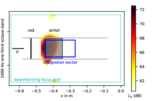
The acoustic measurements were performed with a planar microphone array, consisting of 38 omnidirectional 1/4th inch electret microphone capsules, which have a frequency range from 20 Hz to 20 kHz. They were flush-mounted into an aluminium plate with dimensions of 1.5 m × 1.5 m in the layout shown in Fig. 1. The microphone array was positioned out of the flow in a distance of approximately 0.72 m above the rod and the airfoil. The data were recorded with a sampling frequency of 51.2 kHz and a duration of 40 s using a 24 Bit National Instruments multichannel frontend. In post-processing, which was done using the open source software package Acoular from [24], the data was transferred to the frequency domain by a Fast Fourier Transformation (FFT) on blocks of 4,096 samples, using a Hanning window and an overlap of 50 % according to the method of [25]. The resulting spectra were then averaged to yield the cross-spectral matrix and further processed using the DAMAS beamforming algorithm proposed by [26]. This algorithm, although computationally expensive, is known for its good performance especially at low frequencies (see, for example, the work of [27]) and is often used in aeroacoustic studies (see the comparison by [28]). In the present case, DAMAS was applied to a two-dimensional focus plane parallel to the array, which had an extent of 0.65 m in the streamwise direction and 0.4 m in the spanwise direction. With a high resolution of 0.005 m, this lead to a total of 10,611 grid points. The chosen steering vector was that according to formulation IV in the work of [29]. The result of this beamforming are so-called sound maps, which can be understood as two-dimensional plots of the noise source locations, mapped to the grid points of the beamforming focus grid. As an example, Fig. 2(a) shows such a sound map for one of the experimental cases. Also highlighted in this sound map is the total extent of the beamforming focus grid chosen for this study.
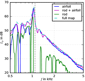
In order to obtain quantitative spectra of the far-field noise generated by the airfoil interacting with the inflow turbulence, an integration sector was defined that contains only the noise contributions due to the interaction of the rod-generated turbulence with the airfoil. It is included both in the schematic (Fig. 1) as well as in the sample sound map (Fig. 2(a)). Background noise sources, such as the rod itself, but also the interaction of the boundary layer along the side walls with the airfoil, were excluded from the integration. Sources due to the interaction of the turbulent boundary layer with the airfoil trailing edge, however, were included. The results were then converted to sound pressure level spectra relative to 20 Pa. Finally, 6 dB were subtracted to account for the refraction at the array plate. To illustrate the need for a suitable integration sector, Fig. 2(b) shows sound pressure level spectra obtained from the integration over various sectors, including a sector that only contains the airfoil (which was the one chosen for the processing of the experimental data), a sector that contains both the airfoil and the cylinder, a sector that contains the cylinder only and a sector that contains the full beamforming focus grid and hence all noise sources. It is visible that the vortex shedding from the cylinder leads to strong tonal noise at a frequency of approximately 1.1 kHz, a component that is also visible in the spectrum obtained from integration over the airfoil sector only. The broadband noise above this tonal peak, however, is mainly generated at the leding edge of the airfoil. Figure 2(b) also contains a theoretical value of the vortex shedding frequency, obtained using a Strouhal number of 0.21. This value was taken from the work of [30].
3 Numerical Setup
3.1 Method
Hybrid RANS/LES methods are becoming increasingly popular to compute unsteady detached flows with reasonable performance in terms of efficiency and accuracy. RANS/LES zonal methods rely on two different models, a RANS model and a subgrid-scale model, which are applied in different domains separated by a sharp or dynamic interface, whereas non-zonal methods assume that the governing set of equations is smoothly transitioning from a RANS behaviour to an LES behaviour, based on criteria updated during the computation. The Detached Eddy Simulation approach (DES) was proposed by [31]. The original DES proposed combines the RANS and LES in a non-zonal manner. In DES, the length scale is replaced by a modified length scale, , which is the minimum between the distance to the wall and a length proportional to the local grid spacing. It is represented mathematically as
| (1) |
| (2) |
where is the distance to the wall, is the local maximum grid spacing and is the model constant calibrated for isotropic turbulence [32]. The original DES length scale, , can become smaller than the boundary layer thickness, leading to an \sayambiguous grid density condition for the original DES and erroneous activation of the LES mode within the attached boundary layer. Therefore, [33] proposed an improved DES method known as delayed DES to solve the grid-induced separation (GIS) and modeled stress depletion (MSD) problems. The modified length scale
| (3) |
is used for the DDES model, where
| (4) |
with being the kinematic eddy viscosity, the molecular viscosity, the velocity gradient and the Karman constant. In the present work, the solutions of the unsteady Reynolds Average Navier-Stokes (URANS) is carried out using a one-equation Spalart–Allmaras model [34] for calculating the turbulent viscosity. Away from the wall, the model is transformed into a Smagorinsky LES Sub-Grid Scale (SGS) model [35]. For the current work, SU2 [36], an open source suite written in C++ and Python to numerically solve partial differential equations (PDE) is used. For spatial integration, a second-order finite volume scheme is applied on the unstructured grids in SU2 using a standard edge-based data structure on a dual grid with control volumes constructed using a median-dual, vertex-based scheme [37]. A dual time-stepping strategy [38] is implemented to achieve a high-order temporal accuracy. In this method, the unsteady problem is converted, at each physical time step, into a series of steady problems, which can then be solved for steady problems using convergence acceleration techniques. For detailed explanation of spatial and temporal integration, please refer to [37].
3.2 Acoustic Solver
In the framework of the present work, the near-field aerodynamic sources are post-processed to the far-field acoustic pressure using the FWH equations [7, 39], which can be written in time domain as
| (5) | ||||
where is the acoustic pressure, is the compressive stress tensor, is the surface normal directed into the fluid, and the retarded time is with the speed of sound . The quantity is called Lighthill’s stress tensor. The above equation is the general form, which can then be modified to account for different operating conditions. The first term, the volume integral, is referred to as the quadrupole term. For low Mach number flows , the volume source terms of quadrupole order are negligible compared to the surface source terms that are of dipole order [40]. Hence, the quadrupole term is ignored in the evaluation of Eq. (5) for the calculations presented in this paper. The last integral corresponds to a monopole sound field generated by the sound energy flux through the surface . If the surface is rigid or impenetrable (and of course stationary) then this term is zero. Validation of the current FWH implementation is included in [41, 42].
In the present approach, the flow solver computes the unsteady flow in the computational domain to give the fluctuating flow variables at each time step on the surface points. The acoustic pressure is then calculated in the time-domain by numerically integrating along the FWH surface for each observer location . In order to compare the broadband predictions based on 2D simulations to the problem of sound radiation from a 3D wing of finite span, additional corrections have to be added to the simulated 2D spectra. Ewert et al. [43] proposed a simple correction formula as
| (6) |
where [44], is the span width and is the 2D polar radius vector in the midspan -plane. It basically denotes the distance to the observer located in the xy-plane at , i.e. .
3.3 Geometrical Description
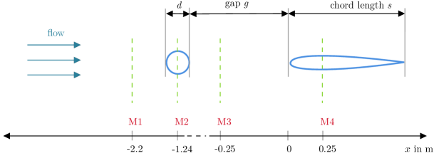
As described above, the rod-airfoil-configuration is a well known and well described problem in aeroacoustics. In a comprehensive analysis published by Zdravkovich [45], the significance of the study of this configuration is well established. The first experimental analysis of this problem by Jacob et al. [5] was performed in order to develop an academic benchmark to test state of the art CAA/CFD techniques. In Fig. 3, the schematic diagram of the configuration to be analysed can be seen, which is consistent with the experimental setup described before. A symmetric NACA 0012 airfoil with a chord length of 100 mm is located downstream of a rod, both extending 120 mm in the spanwise -direction. The origin of the Cartesian coordinate system is located at the mid-span position of the airfoil leading edge. Two cylindrical rods with diameters of 5 mm and 16 mm and lengths of 120 mm are used to generate turbulence. The streamwise gap between rod and airfoil, , was set to 86 mm and 124 mm. Simulations are performed at M=0.076 and M=0.21. Corresponding Reynolds numbers are listed in Table 2. A total of 8 cases were tested.
3.3.1 Computational Domain
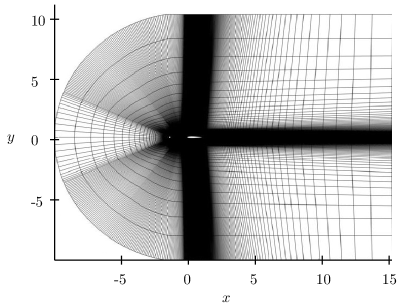
A two-dimensional computational domain for the configuration was constructed that stretched 20 chord lengths, 20 upstream of the rod, 20 downstream of the airfoil, and 10 to each side side of the rod as shown in Fig. 4. The left side of the boundary was set as a velocity inlet, the upper and the lower boundaries as ambient walls, and the right side as pressure outlet. A fine resolution mesh near the rod and airfoil wall was generated with =1.0. A pointwise mesh generation program was used to generate a fully unstructured grid. Corresponding to the experiments and the benchmark, the airfoil was positioned at an angle of attack of zero degrees. To resolve the boundary layer efficiently, an O-type grid and a C-type grid was generated around the rod and the airfoil, respectively. For the mesh elements between the rod and airfoil, the aspect ratio was near unity with an almost constant grid spacing. The resulting computational mesh consists of 1.1 million cells with 300 points around the rod and 400 points around the airfoil in the circumferential direction.
| case | (mm) | (mm) | U (m/s) | airfoil type | ||||
| 1 | 5 | 86 | 26 | NACA 0012 | 0.076 | 0.192 | ||
| 2 | 5 | 86 | 72 | NACA 0012 | 0.210 | 0.219 | ||
| 3 | 5 | 124 | 26 | NACA 0012 | 0.076 | 0.192 | ||
| 4 | 5 | 124 | 72 | NACA 0012 | 0.210 | 0.219 | ||
| 5 | 16 | 86 | 26 | NACA 0012 | 0.076 | 0.195 | ||
| 6 | 16 | 86 | 72 | NACA 0012 | 0.210 | 0.222 | ||
| 7 | 16 | 124 | 26 | NACA 0012 | 0.076 | 0.195 | ||
| 8 | 16 | 124 | 72 | NACA 0012 | 0.210 | 0.222 |
In order to test whether the disagreement between the experiment and the simulation can be mainly attributed to the fact that three-dimensional flow structures in the incoming flow cannot be correctly reproduced by a 2D simulation, a three-dimensional simulation was performed for all the cases on a 3D mesh with 100 parallel planes spanning 3 rod diameters. The cell size in between the airfoil and the rod is 0.02 , with 1 at the walls and periodic condition applied on the spanwise direction. The calculation was performed in the double-time method using a time step of 0.02 with 40 inner iterations per time step. The simulations were conducted on 200 cores.
4 Numerical Aerodynamic Results
4.1 Flow Features
The first step of the analysis is a qualitative study of the fully developed flow in both 2D and 3D flow simulations. The resulting vortex shedding is captured as periodic oscillations in the wake of the rods. In general, in a two-dimensional simulation a common Kármán vortex shedding should be observed because the effect of the span is not present to prevent a regular pattern from forming. Fig. 5 shows the resulting vortex shedding as periodic oscillations in the wake of the rod for case 6 listed in Table 2 ( mm, mm, ). The non-dimensional shedding frequency, based on the rod diameter, derived from the DDES simulation is =0.23, which is slightly higher than the value of 0.21 found in the literature (see, for example, the work of [30]). Greschner et al. [15] explained that the location of the separation point is not determined precisely due to the simple turbulence models in DES, a fact that results in an overpredicted shedding frequency. This could be a potential reason for the disagreement observed in the present study. Fig. 5 further shows that the vortices shed from the rod are convected downstream towards the leading edge of the airfoil. The larger turbulent structures contained in the wake break down while impinging on the leading edge, whereas the smaller eddies go along the airfoil sides and undergo a distortion.

For the 3D simulation, Fig. 6 shows the iso-surfaces of the instantaneous vorticity-field coloured by the Q-criterion. The Kármán vortex street gradually breaks into small vortices in the wake of the rods, and collides with the leading edge of the airfoil. The dissipation reduces the strength of the vortex with increasing downstream distance.
4.2 Velocity Profile Comparisons
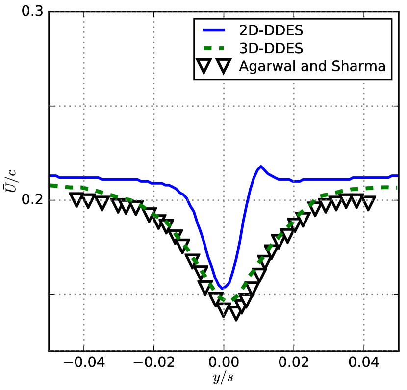
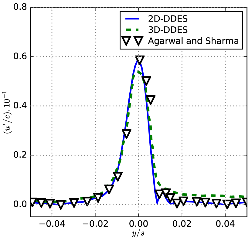
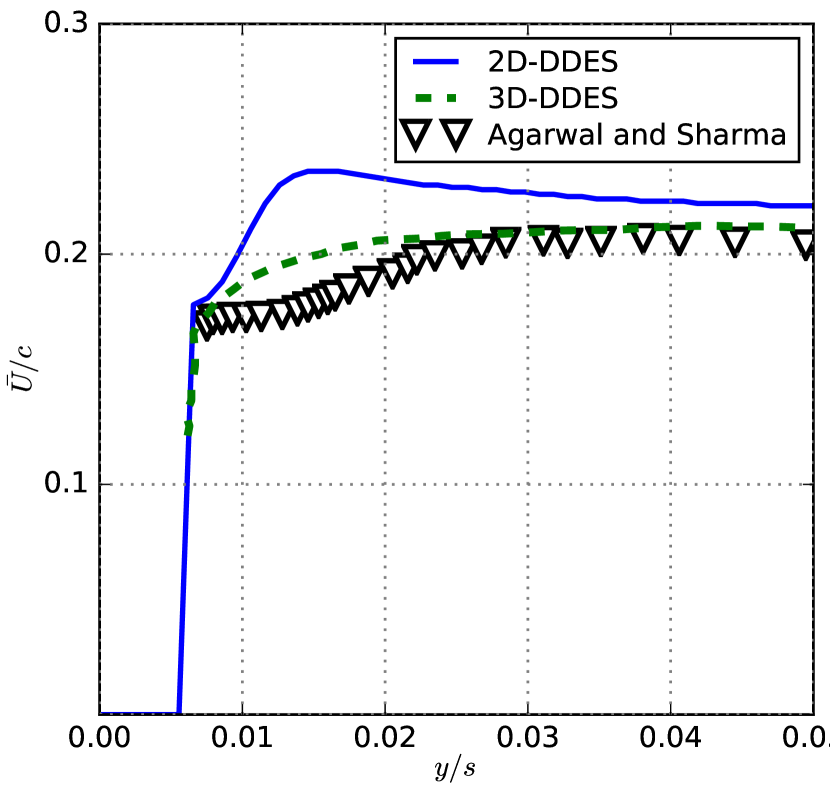
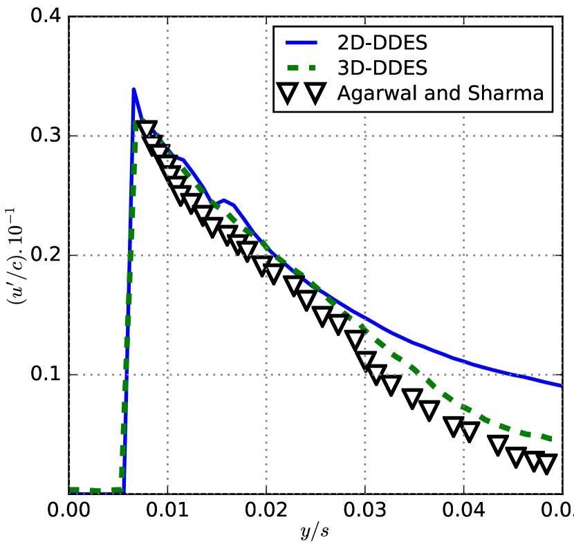
To enable comparisons of the mean and root mean square velocity profiles with outcomes described by [11], 2D and 3D numerical computations were conducted on an additional case ( = 10 mm, = 100 mm, = 100 mm, = 0.2, NACA 0012). The data were sampled for four periods of wake shedding for the numerical simulation. The velocity profiles were extracted at four different streamwise locations, marked as M1 through M4 in the schematic shown in Fig. 3.
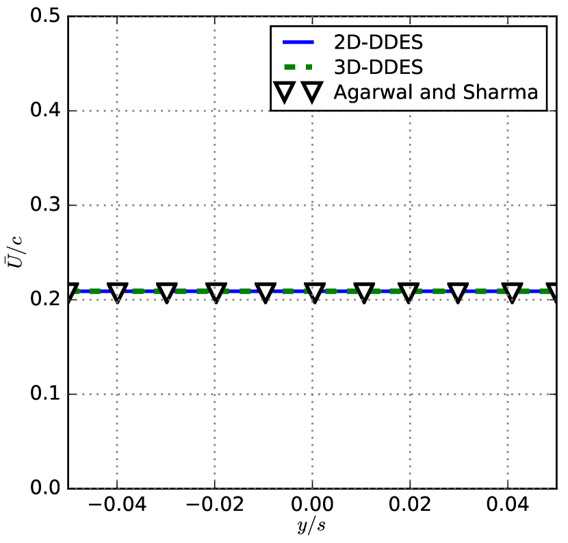
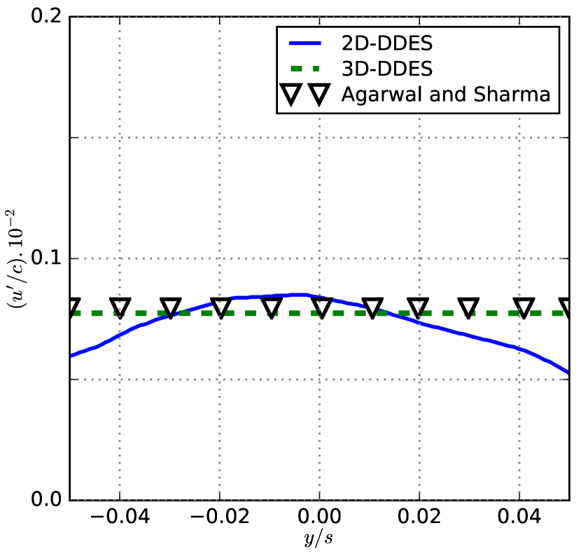
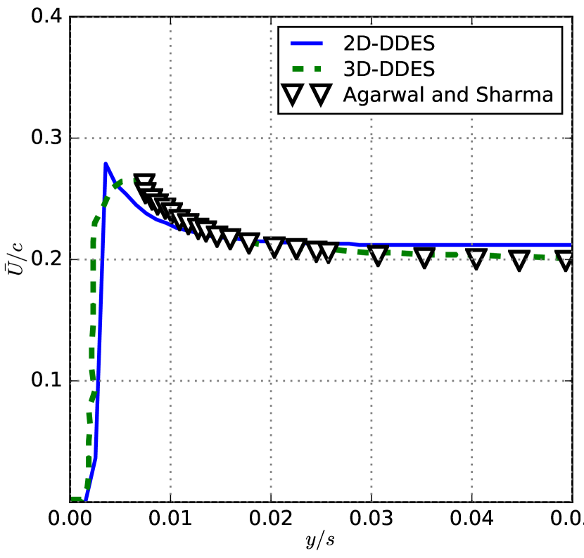
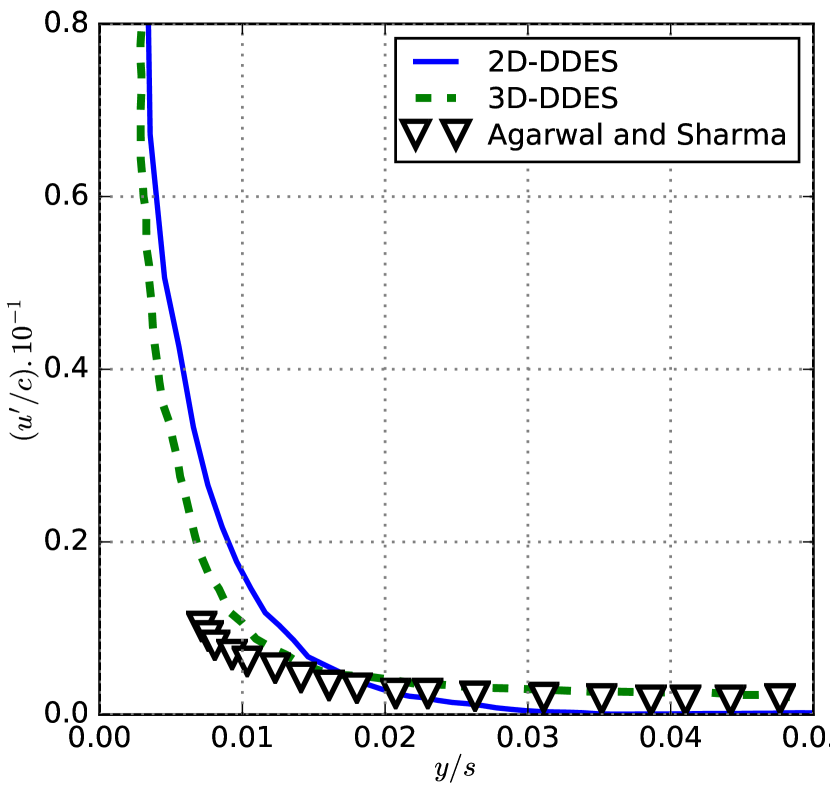
The streamwise mean and fluctuating velocities are extracted at the M1 marker at = -2.2, which is upstream of the rod, and are compared with the experimental work by [11] as shown in Figs. 7(a) and 7(b). The velocities, basically the conditions of the free stream, are clearly predicted by the DDES. The velocity profiles at M2 ( = -1.24), which bisects the rod into equal segments, are shown in Figs. 7(c) and 7(d). The profiles derived from the simulations are again in good agreement with the experiments. The velocity profiles at M3 ( =-0.25) and M4 ( =0.25) are shown in Figs. 8(a)-8(b) and Figs. 8(c)-8(d), respectively. The mean velocity at M3 (upstream of the airfoil) is slightly overpredicted, whereas the rms values of the fluctuating speed are in line with the experimental data at this location. In general, this demonstrates that, as shown earlier by Greschner et al. [15], the 3D-DDES findings are consistent with the experimental data. The rod wake turbulence due to its high intensity and length scale determines the velocity profiles on the airfoil rather than the boundary layer development [46]. It is not surprising that a purely 2D simulation result differs significantly from measurements. Numerically, the flow does not have a third dimension to go to so the levels of fluctuation tend to be much too strong compared to a 3D simulation and measurements. This is consistent with the fact that there is no 2D turbulence. In DES, away from the wall, the active mode is LES mode where 3D turbulence is supposed to freely develop – but it can’t because there is no third dimension and the effect of the turbulence model is very weak because the SGS drives up the destruction term in the turbulence model. So in that region, 2D simulations can be wrong as reported by [32, 47].
5 Aeroacoustic Results
In the first part of this section, the results from the experiments will be discussed. In the second part, the post-processed data obtained from the CFD solver using the FWH solver will be evaluated and the acoustic results from the simulations will be compared with the experimental ones.
5.1 Experimental Results
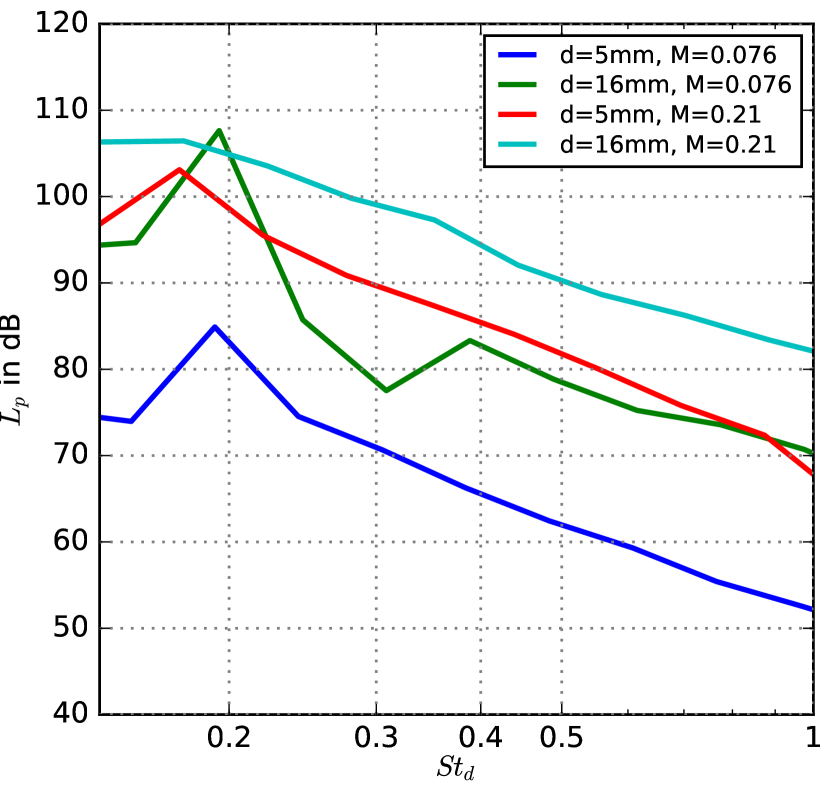
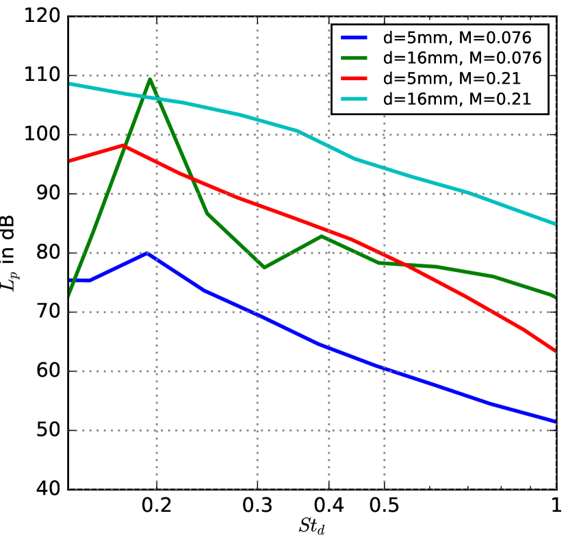
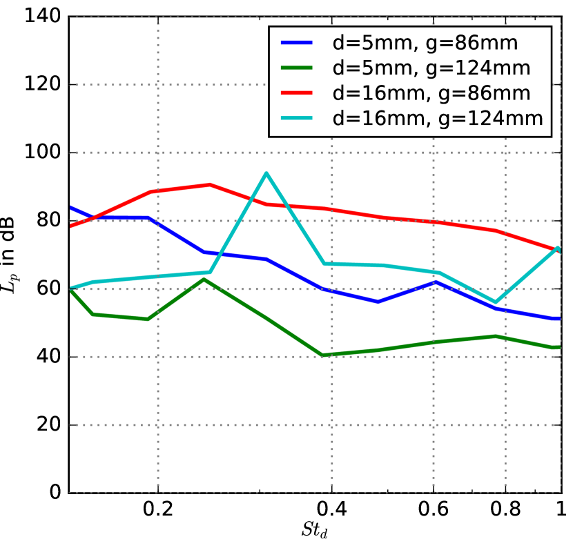
The experimental results obtained for the configurations summarized in Table 2 are shown as 1/3 octave-band sound pressure levels in Fig. 9 and 10. As was already observed in Fig. 2(b), each spectrum exhibits a tonal peak at the 1/3 octave-band that contains the vortex shedding tone of the rod. This is due to the fact that the periodic Kármán vortices shed by the upstream rod interact with the airfoil leading edge. Regarding the broadband noise, notable differences are visible depending on the exact configuration, meaning the cylinder diameter and the gap width .
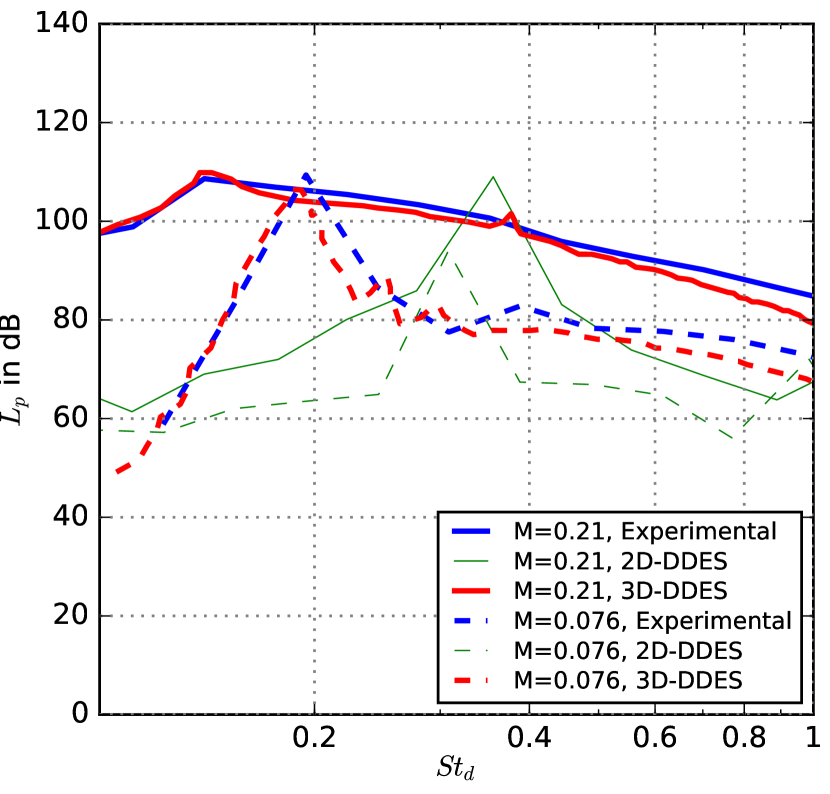
5.1.1 Effect of rod diameter ():
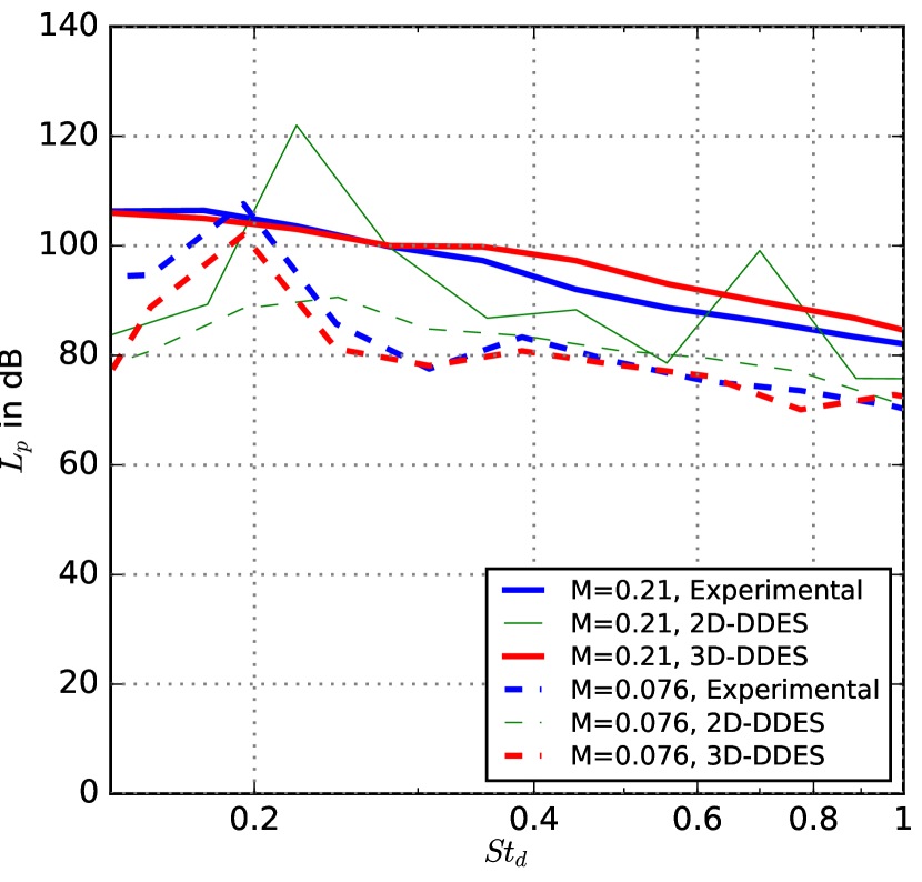
The sound spectra in Fig. 9 show that the dominant frequency is close to the rod vortex shedding frequency and the corresponding Strouhal number is about 0.2. For the small rod with a diameter of 5 mm with mm, it can be clearly seen that the peak levels are 85 dB and 103 dB at =0.076 and =0.21, respectively. In the case of the 16 mm diameter rod, the peak levels are 108 dB and 106 dB at = 0.076 and = 0.21, respectively. These results indicate that the intensity of the vortex-structure interaction at the airfoil leading edge decreases with decreasing rod diameter. In some ways this corresponds to the noise reduction when the airfoil thickness is increased [48, 21]. The similar behaviour can be observed with mm. The observation that the cases with a rod of smaller diameter emit less noise can be justified by the theory of rapid distortion that says that the vortices shed from the smaller rod are less deformed when passing through the leading edge of the airfoil [49]. This results in smaller pressure fluctuations on the surface of the airfoil.
5.1.2 Effect of streamwise gap ():
When looking at cases with identical rod diameter, but different gap width in Fig. 10, a strange observation can be made: For the thinner rod diameter of 5 mm, the cases with the smaller gap width of 86 mm lead to slightly higher amplitudes, while for the thicker rod diameter of 16 mm, the cases with the larger gap width generate slightly more noise.
In order to obtain a better understanding of the basic trends observed in the experimental results, it is reasonable to consider the relation between the noise generated at the leading edge of an airfoil and the properties of the turbulent inflow. When examining the fundamental turbulence interaction noise prediction model by [50] it can be seen that the turbulence intensity of the inflow has a strong effect on the amplitude of the resulting noise. The integral length scale of the incoming turbulence, on the other hand, will have a strong impact on the spectral shape of the resulting far field noise, but only a small effect on its amplitude. An increase in integral length scale, and hence an increase in the size of the turbulent eddies, mainly leads to a broadening of the spectral peak and a shift of this peak towards low frequencies (see, for example, [51]). Since the airfoil was the same in all cases examined here, the observed differences between the broadband content of the measured sound pressure level spectra of the various configurations are a direct result of the corresponding turbulence that hits the airfoil leading edge.
For the cases where the gap width is large compared to the rod diameter, the detailed study by [52] on the turbulence generated by different kinds of grids may be used to shed further light on the turbulence generation. According to this work, the turbulence intensity generated by a grid (including grids that simply consist of a parallel array of circular cylinders) decays with , where is the rod or wire diameter and is the streamwise distance from the grid. Regarding the integral length scale of the turbulence, Roach states that it can be approximated as being proportional to . Hence, the integral length scale increases with increasing distance. However, these approximations are valid only for sufficiently large distances from the grid, where the turbulence can be assumed to be homogeneous and isotropic. In the present investigation, this is most likely true for the small cylinder diameter, for which the ratio of gap width to cylinder diameter, , equals 17.2 for the smaller gap of 86 mm and 24.8 for the larger gap of 124 mm. In both cases, it can be assumed that the turbulence interacting with the leading edge is close to homogeneous. Using the approximations derived by Roach, the cases with the smaller gap width result in a higher turbulence intensity. This, in turn, would lead to a higher sound pressure level according to the model of Amiet, which is exactly what can be seen in the experimental results in Fig. 10(a).
However, for the thicker rod with a diameter of 16 mm, the present gap widths of 86 mm () and 124 mm () mean that the leading edge of the airfoil will be quite close to the airfoil. In this region, the simple approximations given by Roach will not be valid. It is rather likely that the large diameter of the cylinder leads to a large distance between the shear layers on both sides and a large separation bubble. For the cases with the smaller gap width of 86 mm (cases 5 and 6), the airfoil leading edge may be located in a region of reduced turbulence inside the or close to the separation bubble, which explains the lower noise generation. This hypothesis agrees well with results obtained for so-called tandem cylinder configurations [53]. Depending on the distance between the two cylinders, it is possible that the downstream cylinder is located between the shear layers separating from the upstream cylinder (see, for example, [54, 55]).
5.2 Numerical Results and Comparison with Experiments
The far-field spectra of the radiated sound is calculated at the observer’s location at the center of the planar microphone array (0,0,0) (please refer to Fig. 1) using the integration method [7] of Ffowcs Williams and Hawkings with the rigid wall surfaces as the integration surfaces. For low Mach number flows, omitting the quadrupole source has little effect on the noise radiation [40], therefore, dipole sources are examined in the present study. This has been achieved for a complete simulation time of 1.0 s out of which the initial 0.2 s were not considered to eliminate the transients. The FWH surface integrals were calculated for both the circular rod and the airfoil as the sources of sound. However, only the airfoil was considered as the source to compare the results with the experiments. Accordingly, in accordance with [21, 23] the study focuses on the high-frequency component of the spectrum with frequencies greater than the frequency of the vortex shedding from the rod.
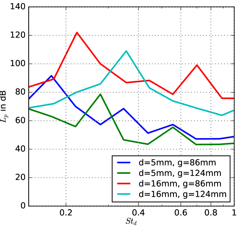
5.2.1 2D-DDES:
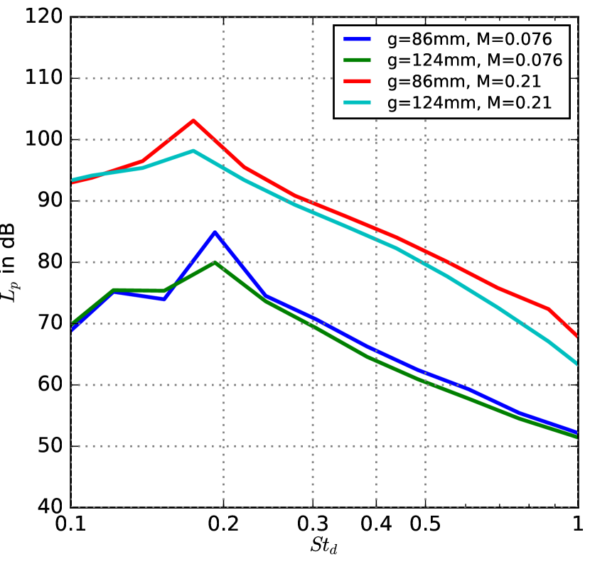
Fig. 11 displays the 1/3 octave-band spectra of the sound pressure levels for all the eight cases from Table 2 as a first summary of the 2D computations. It is clear that the 2D-DDES simulations are incapable of predicting the correct trend of the sound pressure level spectra for all cases. However, surprisingly, the simulations succeeded in finding out which case is yielding higher sound pressure levels and which one results in lower levels. It can be observed from Fig. 11 that case-5 and 7 are emitting higher sound pressure levels compared to case-6 and 8. This is in good agreement with the experimental observations. However, it can be observed that it is not possible to extract the accurate flow physics and acoustics from the two-dimensional simulations, although it still seems possible to identify which rod-airfoil configuration is noisier and which is less.
5.2.2 3D-DDES:
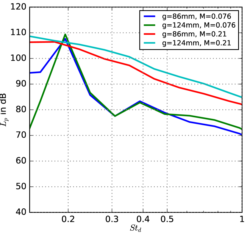
For the three-dimensional simulation, the sound pressure levels obtained from the numerical simulations have to be corrected due to the fact that the set-up spanwise length in the numerical simulations is shorter than the experimental spanwise length . These corrections have been developed by [56, 57, 58] involving the pressure coherence function in the spanwise direction or the spanwise coherence length . As the spanwise coherence length of the cylinder is calculated approximately 2.46, a constant sound pressure level correction of +3.91 dB is added across the whole spectrum.
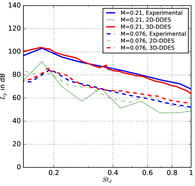
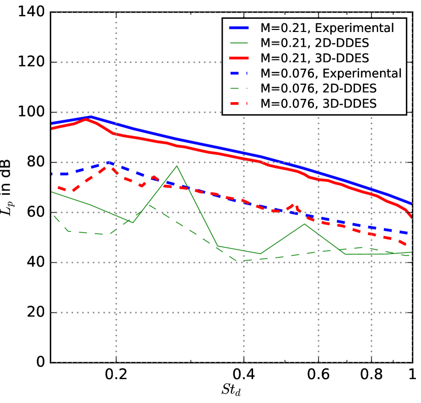
The far-field noise at a position corresponding to the centre of the microphone array, located above the rod and the airfoil configuration (see Fig. 1), obtained from the 2D and 3D simulation is compared with that obtained from the experiments in Fig. 12. In general, the 3D numerical results are able to predict the frequency at the peak of the curve. From that, it can be said that the Kármán vortex shedding region and the stretch and the split of vortices near the leading edge of the airfoil are the primary acoustic source region. The disagreement of 2D acoustic results follows from the fact that 2D simulation of the hydrodynamic field predicts wrong acoustic sources. Typically, in experiment, a long-span test specimen is investigated and the spanwise decorrelation occurs. A good agreement between the experiments and 3D simulations can be observed in all the cases in Fig. 12 because only a 3D scale resolving simulation can capture such 3D noise source. However, it is possible to do 3D flow simulation and then 2D FWH but if the entire aeroacoustic simulation chain is in 2D, then it is necessary to apply empirical corrections before comparing the predicted noise levels to the measured levels.
6 Conclusion
This paper investigates the effects of rod diameter and the streamwise gap between the rod and the leading edge of the airfoil on the noise generated by a rod–airfoil configuration. Experimental measurements and numerical simulations are conducted on eight cases of rod–airfoil configurations at two flow speeds, where the geometric parameters were varied by changing the rod diameter () and the streamwise gap () between the rod and the leading edge of the airfoil. The general conclusions are as follows:
-
1.
For massively separated turbulent flows, DDES is adopted and validated with the LES results. The far-field acoustic prediction using the FWH approach shows good agreement with the experimental data.
-
2.
The sound pressure levels are highly dependent on the geometric parameters. The radiated noise increases with increasing rod diameter and/or shortening the streamwise gap for a thinner rod, while for the thicker rod diameter the larger streamwise gap generate slightly more noise.
-
3.
It was also found that 2D simulations can only predict a very basic spectral shape and trends of sound pressure levels observed in the experiments. The simulated sound pressure levels are usually lower than those measured in experiments.
Acknowledgements
The authors thank Erik W. Schneehagen and Ennes Sarradj from TU Berlin and Andreas Krebs from BTU Cottbus for their help with the three-dimensional simulations.
Appendix A Appendix
Kato’s formula, which assumes that the coherence function has the form of a boxcar function, is given by
| (7) |
| (8) | ||||
| (9) |
According to [56], SPL correction for the long span can be made by adding ,if a coherence length of the surface pressure fluctuations, is determined less than the simulated span. The equivalent coherence length, , can be obtained by calculating the coherence function of the fluctuating wall pressure which is given by
| (10) |
where and are pressure fluctuations (frequency domain) at different span positions on the cylinder surface. The cross-power spectrum can be evaluated with the surface pressure, using the Curle’s analogy solution
| (11) |
For a compact source or when the observer’s position is very far, it can be assumed that constant. Then, the cross-power spectrum is analytically written as
| (12) |
and the acoustic spanwise coherence function can be expressed as
| (13) |
where is the surface pressure at each subsection and is the surface integral over each sub-sectional area. Eq. (12) is the relation between the acoustic spanwise coherence function, and the spanwise coherence function of the ‘integrated’ surface pressure. Using above equation, the coherence length is defined as
| (14) |
References
- Blake [1986] W. K. Blake, Mechanics of Flow-Induced Sound and Vibration, Volume II: Complex Flow-Structure Interactions, Academic Press, Inc., 1986.
- Schulten [1997] J. B. Schulten, Vane sweep effects on rotor/stator interaction noise, AIAA Journal 35 (1997) 945–951.
- Cooper and Peake [2005] A. J. Cooper, N. Peake, Upstream-radiated rotor-stator interaction noise in mean swirling flow, Journal of Fluid Mechanics 523 (2005) 219–250.
- Cooper and Peake [2006] A. J. Cooper, N. Peake, Rotor-stator interaction noise in swirling flow: Stator sweep and lean effects, AIAA Journal 44 (2006) 981–991.
- Jacob et al. [2005] M. C. Jacob, J. Boudet, D. Casalino, M. Michard, A rod-airfoil experiment as a benchmark for broadband noise modeling, Theoretical and Computational Fluid Dynamics 19 (2005) 171–196.
- Casalino et al. [2003] D. Casalino, M. Jacob, M. Roger, Prediction of Rod-Airfoil Interaction Noise Using the Ffowcs-Williams-Hawkings Analogy, AIAA Journal 41 (2003) 182–191.
- Ffowcs Williams and Hawkings [1969] J. E. Ffowcs Williams, D. L. Hawkings, Sound generation by turbulence and surfaces in arbitrary motion, Philosophical Transactions for the Royal Society of London. Series A, Mathematical and Physical Sciences (1969) 321–342.
- Boudet et al. [2005] J. Boudet, N. Grosjean, M. C. Jacob, Wake-Airfoil Interaction as Broadband Noise Source: A Large-Eddy Simulation Study, International Journal of Aeroacoustics 4 (2005) 93–115.
- Berland et al. [2010] J. Berland, P. Lafon, F. Crouzet, F. Daude, C. Bailly, Numerical Insight into Sound Sources of a Rod-Airfoil Flow Configuration Using Direct Noise Calculation, in: 16th AIAA/CEAS Aeroacoustics Conference, 2010.
- Giret et al. [2012] J.-C. Giret, A. Sengissen, S. Moreau, M. Sanjosé, J.-c. Jouhaud, Prediction of the sound generated by a rod-airfoil configuration using a compressible unstructured LES solver and a FW-H analogy, 2012. doi:10.2514/6.2012-2058.
- Agrawal and Sharma [2016] B. R. Agrawal, A. Sharma, Numerical analysis of aerodynamic noise mitigation via leading edge serrations for a rod–airfoil configuration, International Journal of Aeroacoustics 15 (2016) 734–756.
- Jiang et al. [2015] Y. Jiang, M. L. Mao, X. G. Deng, H. Y. Liu, Numerical investigation on body-wake flow interaction over rod-airfoil configuration, Journal of Fluid Mechanics 779 (2015) 1–35.
- Zhiyin [2015] Y. Zhiyin, Large-eddy simulation: Past, present and the future, 2015. doi:10.1016/j.cja.2014.12.007.
- Geyer et al. [2018] T. F. Geyer, S. Sharma, E. Sarradj, Detached Eddy Simulation of the Flow Noise Generation of Cylinders with Porous Cover, in: 2018 AIAA/CEAS Aeroacoustics Conference, AIAA paper 2018-3472, 2018.
- Greschner et al. [2004] B. Greschner, F. Thiele, D. Casalino, M. Jacob, Influence of Turbulence Modeling on the Broadband Noise Simulation for Complex Flows, in: 10th AIAA/CEAS Aeroacoustics Conference, 2004.
- Zhou et al. [2017] B. Zhou, T. A. Albring, N. R. Gauger, C. Ilario, T. D. Economon, J. J. Alonso, Reduction of airframe noise components using a discrete adjoint approach, in: 18th AIAA/ISSMO Multidisciplinary Analysis and Optimization Conference, AIAA paper 2017-3658, 2017.
- Galdeano et al. [2010] S. Galdeano, S. Barré, N. Réau, Noise radiated by a rod-airfoil configuration using DES and the Ffowcs-Williams & Hawkings’ analogy, in: 16th AIAA/CEAS Aeroacoustics Conference, AIAA paper 2010-3702, 2010.
- Greschner et al. [2008] B. Greschner, F. Thiele, M. C. Jacob, D. Casalino, Prediction of sound generated by a rod–airfoil configuration using EASM DES and the generalised Lighthill/FW-H analogy, Computers & Fluids 37 (2008) 402–413.
- Caraeni et al. [2007] M. Caraeni, Y. Dai, D. Caraeni, Acoustic Investigation of Rod Airfoil Configuration with DES and FWH, in: 37th AIAA Fluid Dynamics Conference and Exhibit, AIAA paper 2007-4106, 2007.
- Gerolymos and Vallet [2007] G. A. Gerolymos, I. Vallet, Influence of Temporal Integration and Spatial Discretization on Hybrid RSM-VLES Computations, in: 18th AIAA Computational Fluid Dynamics Conference, AIAA paper 2007-4094, 2007.
- Giesler and Sarradj [2009] J. Giesler, E. Sarradj, Measurement of broadband noise generation on rod-airfoil-configurations, in: 15th AIAA/CEAS Aeroacoustics Conference (30th AIAA Aeroacoustics Conference), AIAA paper 2009-3308, 2009.
- Sarradj et al. [2009] E. Sarradj, C. Fritzsche, T. F. Geyer, J. Giesler, Acoustic and aerodynamic design and characterization of a small-scale aeroacoustic wind tunnel, Applied Acoustics 70 (2009) 1073–1080.
- Giesler [2011] J. Giesler, Schallentstehung durch turbulente Zuströmung an aerodynamischen Profilen, Doctoral thesis, Brandenburg University of Technology, Cottbus, 2011.
- Sarradj and Herold [2017] E. Sarradj, G. Herold, A python framework for microphone array data processing, Applied Acoustics 116 (2017) 50–58.
- Welch [1967] P. Welch, The use of fast fourier transform for the estimation of power spectra: a method based on time averaging over short, modified periodograms, IEEE Transactions on audio and electroacoustics 15 (1967) 70–73.
- Brooks and Humphreys [2006] T. F. Brooks, W. M. Humphreys, A deconvolution approach for the mapping of acoustic sources (DAMAS) determined from phased microphone arrays, Journal of Sound and Vibration 294 (2006) 856–879.
- Herold and Sarradj [2017] G. Herold, E. Sarradj, Performance analysis of microphone array methods, Journal of Sound and Vibration 401 (2017) 152–168.
- Merino-Martinez et al. [2019] R. Merino-Martinez, P. Sijtsma, M. Snellen, T. Ahlefeld, J. Antoni, C. J. Bahr, D. Blacodon, D. Ernst, A. Finez, S. Funke, T. F. Geyer, S. Haxter, G. Herold, X. Huang, W. M. Humphreys, Q. Leclère, A. Malgoezar, U. Michel, T. Padois, A. Pereira, C. Picard, E. Sarradj, H. Siller, D. G. Simons, C. Spehr, A review of acoustic imaging methods using phased microphone arrays, CEAS Aeronautical Journal (2019) 1–34.
- Sarradj [2012] E. Sarradj, Three-dimensional acoustic source mapping with different beamforming steering vector formulations, Advances in Acoustics and Vibration 2012 (2012).
- Schlichting and Gersten [1997] H. Schlichting, K. Gersten, Boundary-layer theory, 9th edition ed., Springer Science+Business Media, Berlin, 1997.
- Spalart et al. [1997] P. R. Spalart, W. H. Jou, M. K. Strelets, S. R. Allmaras, Comments on the feasibility of LES for wings and on a hybrid RANS/LES approach, Advances in DNS/LES 1 (1997) 4–8.
- Spalart [2009] P. R. Spalart, Detached-eddy simulation, Annual Review of Fluid Mechanics 41 (2009) 181–202.
- Spalart et al. [2006] P. R. Spalart, S. Deck, M. L. Shur, K. D. Squires, M. K. Strelets, A. Travin, A new version of detached-eddy simulation, resistant to ambiguous grid densities, Theoretical and Computational Fluid Dynamics 20 (2006) 181–195.
- Spalart and Allmaras [1992] P. R. Spalart, S. R. Allmaras, A one-equation turbulence model for aerodynamic flows (1992).
- Smagorinsky [1963] J. Smagorinsky, General circulation experiments with the primitive equations: i. The basic experiment, Monthly Weather Review 91 (1963) 99–164.
- Economon et al. [2015] T. D. Economon, F. Palacios, S. R. Copeland, T. W. Lukaczyk, J. J. Alonso, Su2: An open-source suite for multiphysics simulation and design, Aiaa Journal 54 (2015) 828–846.
- Molina et al. [2017] E. Molina, C. Spode, R. G. Annes da Silva, D. E. Manosalvas-Kjono, S. Nimmagadda, T. D. Economon, J. J. Alonso, M. Righi, Hybrid rans/les calculations in su2, in: 23rd AIAA Computational Fluid Dynamics Conference, AIAA paper 2017-4284, 2017.
- Jameson and Shankaran [2009] A. Jameson, S. Shankaran, An assessment of dual-time stepping, time spectral and artificial compressibility based numerical algorithms for unsteady flow with applications to flapping wings (2009).
- Farassat [2007] F. Farassat, Derivation of Formulations 1 and 1A of Farassat, Nasa/TM-2007-214853 214853 (2007) 1–25.
- Brentner and Farassat [2003] K. S. Brentner, F. Farassat, Modeling aerodynamically generated sound of helicopter rotors, Progress in Aerospace Sciences 39 (2003) 83 – 120.
- Sharma et al. [2020] S. Sharma, E. Sarradj, H. Schmidt, Stochastic modelling of leading-edge noise in time-domain using vortex particles, Journal of Sound and Vibration (2020) 1–175.
- Sharma [2020] S. Sharma, Stochastic modelling of leading-edge noise in time-domain using vortex particles, Doctoral thesis, BTU Cottbus - Senftenberg, 2020. doi:10.26127/BTUOpen-5085.
- Ewert et al. [2009] R. Ewert, C. Appel, J. Dierke, M. Herr, RANS/CAA Based Prediction of NACA 0012 Broadband Trailing Edge Noise and Experimental Validation, in: 15th AIAA/CEAS Aeroacoustics Conference (30th AIAA Aeroacoustics Conference), American Institute of Aeronautics and Astronautics, Reston, Virigina, 2009. doi:10.2514/6.2009-3269.
- Amiet [1976] R. K. Amiet, Noise due to turbulent flow past a trailing edge, Journal of Sound and Vibration 47 (1976) 387–393.
- Zdravkovich [1997] M. M. Zdravkovich, Flow around circular cylinders: A comprehensive guide through flow phenomena, experiments, applications, mathematical models, and computer simulations, Oxford University Press, 1997.
- Sharma et al. [2019] S. Sharma, T. F. Geyer, E. Sarradj, H. Schmidt, Numerical investigation of noise generation by rod-airfoil configuration using des (su2) and the fw-h analogy, in: 25th AIAA/CEAS Aeroacoustics Conference, 2019. doi:10.2514/6.2019-2400.
- Mockett [2009] C. Mockett, A comprehensive study of detached-eddy simulation, Ph.D. thesis, Technische Universität Berlin, 2009. URL: https://depositonce.tu-berlin.de/handle/11303/2602.
- Gershfeld [2004] J. Gershfeld, Leading edge noise from thick foils in turbulent flows, Journal of the Acoustical Society of America 116 (2004) 1416–1426.
- Li et al. [2014] Y. Li, X. nian Wang, Z. wu Chen, Z. chu Li, Experimental study of vortex-structure interaction noise radiated from rod-airfoil configurations, Journal of Fluids and Structures 51 (2014) 313–325.
- Amiet [1975] R. K. Amiet, Acoustic radiation from an airfoil in a turbulent stream, Journal of Sound and vibration 41 (1975) 407–420.
- Geyer [2018] T. F. Geyer, Motor- und Aggregate-Akustik, 10. Magdeburger Symposium, Otto-von-Guericke-Universität Magdeburg, 2018, pp. 185 – 206. doi:10.24352/UB.OVGU-2018-115.
- Roach [1987] P. E. Roach, The generation of nearly isotropic turbulence by means of grids, International Journal of Heat and Fluid Flow 8 (1987) 82–92.
- Lockard et al. [2007] D. Lockard, M. Khorrami, M. Choudhari, F. Hutcheson, T. Brooks, D. Stead, Tandem cylinder noise predictions, in: 13th AIAA/CEAS Aeroacoustics Conference (28th AIAA Aeroacoustics Conference), 2007, p. 3450.
- Wu et al. [1994] J. Wu, L. Welch, M. Welsh, J. Sheridan, G. Walker, Spanwise wake structures of a circular cylinder and two circular cylinders in tandem, Experimental Thermal and Fluid Science 9 (1994) 299–308.
- Alam [2014] M. M. Alam, The aerodynamics of a cylinder submerged in the wake of another, Journal of Fluids and Structures 51 (2014) 393–400.
- Kato and Ikegawa [1991] C. Kato, M. Ikegawa, Large eddy simulation of unsteady turbulent wake of a circular cylinder using the finite element method, in: Advances in Numerical Simulation of Turbulent Flows, 1991, pp. 49–56.
- Seo and Moon [2007] J. H. Seo, Y. J. Moon, Aerodynamic noise prediction for long-span bodies, Journal of Sound and Vibration 306 (2007) 564–579.
- Moon et al. [2010] Y. J. Moon, J. H. Seo, Y. M. Bae, M. Roger, S. Becker, A hybrid prediction method for low-subsonic turbulent flow noise, Computers and Fluids 39 (2010) 1125–1135.