Adaptive Mesh Refinement and Coarsening for Diffusion-Reaction Epidemiological Models

Abstract

The outbreak of COVID-19 in 2020 has led to a surge in the interest in the mathematical modeling of infectious diseases. Disease transmission may be modeled as compartmental models, in which the population under study is divided into compartments and has assumptions about the nature and time rate of transfer from one compartment to another. Usually, they are composed of a system of ordinary differential equations (ODE’s) in time. A class of such models considers the Susceptible, Exposed, Infected, Recovered, and Deceased populations, the SEIRD model. However, these models do not always account for the movement of individuals from one region to another. In this work, we extend the formulation of SEIRD compartmental models to diffusion-reaction systems of partial differential equations to capture the continuous spatio-temporal dynamics of COVID-19. Since the virus spread is not only through diffusion, we introduce a source term to the equation system, representing exposed people who return from travel. We also add the possibility of anisotropic non-homogeneous diffusion. We implement the whole model in libMesh, an open finite element library that provides a framework for multiphysics, considering adaptive mesh refinement and coarsening. Therefore, the model can represent several spatial scales, adapting the resolution to the disease dynamics. We verify our model with standard SEIRD models and show several examples highlighting the present model’s new capabilities.

Keywords COVID-19  $\cdot$ Compartmental models  Diffusion-reaction  $\cdot$ Partial differential equations  $\cdot$ Adaptive mesh refinement and coarsening

1 Introduction

The COVID-19 pandemic has caused widespread damage worldwide, in terms of human lives and international economic weakening. As a new highly contagious disease, governments have taken unprecedented measures to slow the spread of the virus, including quarantines, curfews, lockdowns, and national and international travel suspension. These measures, considered essential by many experts, are partly motivated by the lack of reliable data on this disease’s transmission and lethality, which justifies cautious responses from the authorities and population. These events demonstrate more than ever the need for reliable tools designed to model the spatio-temporal spread of infectious diseases.

The study of infectious disease proliferation is a well-established field and has given rise to the area of science called mathematical epidemiology [1]. Mathematical epidemiology proposes models that help the understanding of epidemics and to outline policies to control infectious diseases. In Brazil, studies of this type have been carried out for years for diseases such as Dengue [2] and Zika [3], and, in a global context, diseases such as HIV [4], SARS [5], Malaria [6], Ebola [7], among others. The COVID-19 pandemic brought the need for more research in this area. Several models for this pandemic outbreak have been presented in recent months [8, 9, 10, 11, 12, 13].

Disease transmission may be modeled as compartmental models, in which the population under study is divided into compartments and has assumptions about the nature and time rate of transfer from one compartment to another [14]. These models have been used extensively in biological, ecological, and chemical applications [15, 16, 17]. They allow for an understanding of the processes at work and for predicting the dynamics of the epidemic.

The large majority of the compartmental models are composed of a system of ordinary differential equations (ODE’s) in time. Though compartmentalized models are simple to formulate, analyze, and solve numerically, these models do not always account for the movement of individuals from one region to another. Different approaches have been used to introduce spatial variation into such ODE models [18, 19, 20, 11]. The strategies consist of defining regional compartments corresponding to different geographic units and adding coupling terms to the model equations to account for species’ movement from unit to unit.

In this work, we use a partial differential equation (PDE) model to capture the continuous spatio-temporal dynamics of COVID-19. PDE models incorporate spatial information more naturally and allow for capture the dynamics across several scales of interest. They have a significant advantage over ODE models, whose ability to describe spatial information is limited by the number of geographic compartments. Indeed, recent research indicates that COVID-19 spreading presents multi-scale features that go from the virus and individual immune system scale to the collective behavior of a whole population [21]. We study a compartmental SEIRD model (susceptible, exposed, infected, recovered, deceased) that incorporates spatial spread through diffusion terms [16, 22, 8, 9, 23]. Adaptive mesh refinement and coarsening [24] can resolve population dynamics from local (street, city) to regional (district, state), providing an accurate spatio-temporal description of the infection spreading. Moreover, diffusion may be properly tuned to account for local natural or social inhomogeneities (e.g., mountains, lakes, highways) describing populations’ movements.

However, the main limitation of the diffusion-reaction PDE approach is the definition of the diffusion operator and transmission coefficients, which depend on the population’s behavior. Another issue is that the virus spread is not only through diffusion, since people, who may be infected, travel long distances in a short period. Some models relate the mobile geolocation data with the spread of the disease [25, 26]. These issues make the model a highly complex system, which may completely change as the population’s behavior changes. Therefore, this work contributes to improving the knowledge of compartmental diffusion-reaction PDE models.

All implementations are done using the libMesh library. As other freely available open-source libraries (deal.II [27], FEniCS [28], GRINS [29], MOOSE [30], etc), libmesh provides a finite element framework that can be used for numerical simulation of partial differential equations in various applied fields in science and engineering. It has already been used in more than 1,000 publications with applications in many different areas. See, for example, recent applications in sediment transport [31] and bubble dynamics [32]. This library is an excellent tool for programming the finite element method and can be used for one-, two-, and three-dimensional steady and transient simulations on serial and parallel platforms. The libmesh library provides native support for adaptive mesh refinement and coarsening, thus providing a natural environment for the present study. The main advantage of this library is the possibility of focusing on implementing the specifics features of the modeling without worrying about adaptivity and code parallelization. Consequently, the effort to build a high performance computing code tends to be minimized. about adaptivity and code parallelization.

The remainder of this work is organized as follows: In section 2, we present the governing equations that describe the dynamics of a virus infection. First, we present a generic spatio-temporal SEIRD model, based on the EPIDEMIC software [33], used to verify our implementation. We then present a model that better represents the dynamics of COVID-19 infection spread, based on [9, 8]. In section 3, we introduce the Galerkin finite element formulation, the time discretization, and the libMesh implementation. Then, we present the numerical verification of the generic spatio-temporal SEIRD model implementation. We verify our algorithm’s capacity to represent a compartmental model [33] and show how the diffusion influences the dynamics. Section 5 presents the numerical results of the spatio-temporal model of COVID-19 infection spread. We perform simulations similar to the ones presented in [8] and show tests to highlight the new modeling capabilities introduced in this work. Finally, the paper ends with a summary of our main findings and the perspectives for the next steps of this research.

2 Governing equations

The presentation of the governing equations follows the continuum mechanics framework in [8] instead of the more traditional approach found in mathematical and biological references. Consider a system which may be decomposed into $N$ distinct populations: $u_{1}(\mathbf{x},t)$, $u_{2}(\mathbf{x},t)$, …, $u_{N}(\mathbf{x},t)$. Let $\Omega\in R^{2}$ be a simply connected domain of interest with boundary $\partial\Omega=\Gamma_{D}\cap\Gamma_{N}$, and $[0,T]$ a generic time interval. The vector compact representation of the governing equations as a transient nonlinear diffusion-reaction system of equations reads,

$$\frac{\partial\mathbf{u}}{\partial t}+\left(\mathbf{A}+\mathbf{B(u)}\right)\mathbf{u}-\nabla\cdot(\boldsymbol{\nu}\nabla\mathbf{u})-\mathbf{f}=0\textrm{ in }\Omega\times[0,T]$$ (1)

$$\mathbf{u}=\mathbf{u_{D}}\textrm{ in }\Gamma_{D}\times[0,T]$$ (2)

$$(\boldsymbol{\nu}\nabla\mathbf{u})\cdot\mathbf{n}=\mathbf{h}\textrm{ in }\Gamma_{N}\times[0,T]$$ (3)

We denote the densities of the susceptible, exposed, infected, recovered and deceased populations as $s(\mathbf{x},t)$, $e(\mathbf{x},t)$, $i(\mathbf{x},t)$, $r(\mathbf{x},t)$, and $d(\mathbf{x},t)$. Also, let $c(\mathbf{x},t)$ denote the cumulative number of infected and $n(\mathbf{x},t)$ the sum of the living population; i.e., $n(\mathbf{x},t)=s(\mathbf{x},t)+e(\mathbf{x},t)+i(\mathbf{x},t)+r(\mathbf{x},t)$. We consider $\mathbf{u}=[s,e,i,r,d]^{T}$. The matrices $\mathbf{A}$, $\mathbf{B}$ and $\boldsymbol{\nu}$, and the vector $\mathbf{f}$ depend on a particular form of the system dynamics. Furthermore, in general, $\boldsymbol{\nu}=\boldsymbol{\nu}(\mathbf{x})$, that is, diffusion is heterogeneous and anisotropic. Besides the boundary conditions (2), (3), we specify the initial condition $\mathbf{u}(\mathbf{x},0)=\mathbf{u}_{0}$. The total population $U_{i}(t)$ of each compartment $u_{i}(\mathbf{x},t)$ is,

$$U_{i}(t)=\int_{\Omega}u_{i}(\mathbf{x},t)d\Omega$$ (4)

for $i=1,2,\cdots,N$.

2.1 Generic spatio-temporal SEIRD model

We first consider a SEIRD model [14] given by the following system of coupled PDEs over $\Omega\times[0,T]$:

$$\frac{\partial s}{\partial t}+\frac{\beta}{n}si-\nabla\cdot(n\nu_{s}\nabla s)=0$$ (5)

$$\frac{\partial e}{\partial t}-\frac{\beta}{n}si+\alpha e-\nabla\cdot(n\nu_{e}\nabla e)=0$$ (6)

$$\frac{\partial i}{\partial t}-\alpha e+(\gamma+\delta)i-\nabla\cdot(n\nu_{i}\nabla i)=0$$ (7)

$$\frac{\partial r}{\partial t}-\gamma i-\nabla\cdot(n\nu_{r}\nabla r)=0$$ (8)

$$\frac{\partial d}{\partial t}-\delta i=0$$ (9)

where $\beta$ is transmission rate $(days^{-1})$, $\alpha$ the latent rate $(days^{-1})$, $\gamma$ the recovery rate $(days^{-1})$, $\delta$ the death rate $(days^{-1})$, and $\nu_{s}$, $\nu_{e}$, $\nu_{i}$, $\nu_{r}$ are diffusion parameters respectively corresponding to the different population groups ($km^{2}persons^{-1}days^{-1}$). We append to the system of equations homogeneous Neumann boundary conditions, that is, $(\boldsymbol{\nu}\cdot\nabla\mathbf{u})\cdot\mathbf{n}=0$.

We can reframe this model in the general form given by equation (1). Thus, the matrices $\mathbf{A}$, $\mathbf{B}$, $\boldsymbol{\nu}$ and the vector $\mathbf{f}$ reads,

$$\mathbf{A}=\begin{bmatrix}0&0&0&0&0\\ 0&\alpha&0&0&0\\ 0&-\alpha&\gamma+\delta&0&0\\ 0&0&-\gamma&0&0\\ 0&0&-\delta&0&0\\ \end{bmatrix}$$ (10)

$$\mathbf{B}=\begin{bmatrix}0&0&\frac{\beta}{n}s&0&0\\ 0&0&-\frac{\beta}{n}s&0&0\\ 0&0&0&0&0\\ 0&0&0&0&0\\ 0&0&0&0&0\\ \end{bmatrix}$$ (11)

$$\boldsymbol{\nu}=\begin{bmatrix}\boldsymbol{\nu_{s}}&0&0&0&0\\ 0&\boldsymbol{\nu_{e}}&0&0&0\\ 0&0&\boldsymbol{\nu_{i}}&0&0\\ 0&0&0&\boldsymbol{\nu_{r}}&0\\ 0&0&0&0&0\\ \end{bmatrix}$$ (12)

$$\boldsymbol{\nu^{k}}=\begin{bmatrix}\nu^{k}_{xx}&\nu^{k}_{xy}\\ \nu^{k}_{yx}&\nu^{k}_{yy}\end{bmatrix}\textnormal{ with }k=s,e,i,r$$ (13)

$$\mathbf{f}=\mathbf{0}$$ (14)

This model is based on the EPIDEMIC software, and it is employed to verify our implementation. The system of equations represents that the susceptible population decreases as the exposed population increases. This variation depends on the transmission rate between infected and susceptible. The number of exposed increases because of the transmission rate and decreases when the exposed individuals become infected (after the incubation period). The number of infected increases after the incubation period and decreases depending on the recovery and death rate. The number of deaths depends only on the death rate as the number of recovered depends only on the recovery rate. Finally, the cumulative number of infected depends only on the exposed and the incubation period. The diffusion parameters are included in the model to spread the disease spatially.

Summarizing, this model assumes:

• Movement is proportional to population size; i.e., more movement occurs within heavily populated regions;

• No movement occurs among the deceased population;

• There is a latency period between exposure and the development of symptoms;

• The probability of contagion is inversely proportional to the population size;

• The exposed persons will ever develop symptoms;

• Only infected persons are capable of spreading the disease;

• The non-virus mortality rate is not considered in this model;

• New births are not considered in this model.

Note that the EPIDEMIC model’s dynamics does not represent the actual COVID19 dynamics since, in the case of COVID19, the exposed population may be asymptomatic and recover without becoming infected and still spread the virus. Thus, a better model would be the one based on [9, 8].

2.2 Spatio-temporal model of COVID-19 infection spread

We begin by making several model assumptions to represent the COVID-19 infection spread adequately [8]:

• Only mortality due the COVID-19 is considered;

• New births are not considered in this model.

• Some portion of exposed persons never develop symptoms, and move directly from the exposed compartment to the recovered compartment (asymptomatic cases);

• Both asymptomatic (exposed) and symptomatic (infected) patients are capable of spreading the disease;

• There is a latency period between exposure and the development of symptoms;

• It is possible that new cases of exposed people appear randomly in the system (exposed people who return from a travel);

• The probability of contagion increases with population size (Allee effect [9]);

• Movement is proportional to population size; i.e., more movement occurs within heavily populated regions;

• No movement occurs among the deceased population;

Then, the system of equations becomes:

$$\frac{\partial s}{\partial t}+\beta_{i}\left(1-\frac{A}{n}\right)si+\beta_{e}\left(1-\frac{A}{n}\right)se+f-\nabla\cdot(n\nu_{s}\nabla s)=0$$ (15)

$$\frac{\partial e}{\partial t}-\beta_{i}\left(1-\frac{A}{n}\right)si-\beta_{e}\left(1-\frac{A}{n}\right)se+(\alpha+\gamma_{e})e-f-\nabla\cdot(n\nu_{e}\nabla e)=0$$ (16)

$$\frac{\partial i}{\partial t}-\alpha e+(\gamma_{i}+\delta)i-\nabla\cdot(n\nu_{i}\nabla i)=0$$ (17)

$$\frac{\partial r}{\partial t}-\gamma_{e}e-\gamma_{i}i-\nabla\cdot(n\nu_{r}\nabla r)=0$$ (18)

$$\frac{\partial d}{\partial t}-\delta i=0$$ (19)

where $A$ characterizes the Allee effect ($persons$), that takes into account the tendency of outbreaks to cluster around large populations, $\beta_{i}$ is the transmission rate between symptomatic and susceptible $(persons^{-1}days^{-1})$, $\beta_{e}$ is the transmission rate between asymptomatic and susceptible $(persons^{-1}days^{-1})$, $f$ is a source function that depends on space and time $(persons)$, $\alpha$ is the latent rate $(days^{-1})$, $\gamma_{e}$ is the recovery rate of the asymptomatic $(days^{-1})$, $\gamma_{i}$ is the recovery rate of the symptomatic $(days^{-1})$, $\delta$ is the death rate $(days^{-1})$, and $\nu_{s}$, $\nu_{e}$, $\nu_{i}$, $\nu_{r}$ are the diffusion parameters respectively corresponding to the different population groups ($km^{2}persons^{-1}days^{-1}$).

Now, we call exposed who has contact with the virus but remains asymptomatic. However, since the virus is highly transmissible, the exposed population also may transmit the virus. The exposed may recover without any symptoms or may become infected. The infected follow the same logic of the previous SEIRD system (they may recover or die). The main difference in the new SEIRD system is in the exposed population and whom it interacts. The source function $f$ may be defined to represent exposed people who return from travel. Note that $\beta$ has units ($days^{-1}$) while $\beta_{i}$ and $\beta_{e}$ have units ($person^{-1}days^{-1}$). While equations (5) and (6) divide $\beta$ by the living population, equations (15), (16) and (17) keep $\beta_{i}$ and $\beta_{e}$ constant independent of that.

Therefore, to express this model in the general form given by equation (1), the matrices $\mathbf{A}$, $\mathbf{B}$, $\boldsymbol{\nu}$ and the vector $\mathbf{f}$ reads,

$$\mathbf{A}=\begin{bmatrix}0&0&0&0&0\\ 0&\alpha+\gamma_{e}&0&0&0\\ 0&-\alpha&\gamma_{i}+\delta&0&0\\ 0&-\gamma_{e}&-\gamma_{i}&0&0\\ 0&0&-\delta&0&0\\ \end{bmatrix}$$ (20)

$$\mathbf{B}=\begin{bmatrix}0&\beta_{e}\left(1-\frac{A}{n}\right)s&\beta_{i}\left(1-\frac{A}{n}\right)s&0&0\\ 0&-\beta_{e}\left(1-\frac{A}{n}\right)s&-\beta_{i}\left(1-\frac{A}{n}\right)s&0&0\\ 0&0&0&0&0\\ 0&0&0&0&0\\ 0&0&0&0&0\\ \end{bmatrix}$$ (21)

$$\boldsymbol{\nu}=\begin{bmatrix}\boldsymbol{\nu_{s}}&0&0&0&0\\ 0&\boldsymbol{\nu_{e}}&0&0&0\\ 0&0&\boldsymbol{\nu_{i}}&0&0\\ 0&0&0&\boldsymbol{\nu_{r}}&0\\ 0&0&0&0&0\\ \end{bmatrix}$$ (22)

$$\boldsymbol{\nu^{k}}=\begin{bmatrix}\nu^{k}_{xx}&\nu^{k}_{xy}\\ \nu^{k}_{yx}&\nu^{k}_{yy}\end{bmatrix}\textnormal{ with }k=s,e,i,r$$ (23)

$$\mathbf{f}=\begin{bmatrix}-f\\ f\\ 0\\ 0\\ 0\\ \end{bmatrix}$$ (24)

If we assume that the region of interest is isolated, we prescribe the following homogeneous Neumann boundary conditions,

$$\nabla s\cdot\mathbf{n}=0$$ (25)

$$\nabla e\cdot\mathbf{n}=0$$ (26)

$$\nabla i\cdot\mathbf{n}=0$$ (27)

$$\nabla r\cdot\mathbf{n}=0$$ (28)

or simply $(\boldsymbol{\nu}\cdot\nabla\mathbf{u})\cdot\mathbf{n}=0$.

2.3 Determination of $R_{0}$

The basic reproduction number, $R_{0}$, is defined as the average number of additional infections produced by an infected individual in a wholly susceptible population over the full course of the disease outbreak. In an epidemic situation, the threshold $R_{0}=1$ is the dividing line between the infection dying out and the onset of an epidemic. $R_{0}>1$ implies growth of the epidemic, whereas $R_{0}<1$ implies decay in infectious spread [14].

The concept of $R_{0}$ is well-defined for ODE models. However, its extension to a PDE model is unclear, owing to the influence of diffusion. Viguerie et al. [8] found that a $R_{0}$ derived for the ODE version of the PDE model is not consistently reliable to represent the epidemic’s dynamic growth adequately. If we do not consider the diffusion, $R_{0}$ may be calculated as:

$$R_{0}=\frac{\beta_{e}s+f}{\alpha+\gamma_{e}}+\frac{\beta_{i}\alpha s}{(\alpha+\gamma_{e})(\delta+\gamma_{i})}$$ (29)

For further details about the $R_{0}$ calculation, refer to [34, 8].

3 Finite Element Formulation

In this section we briefly introduce the Galerkin finite element formulation, the time discretization, and the the libMesh implementation, supporting adaptive mesh refinement and coarsening. Appendices A and B give respectively the resulting finite element matrices for the generic spatio-temporal SEIRD and COVID-19 models.

3.1 Space Discretization

We introduce a Galerkin finite element variational formulation for space discretization. Without loss of generality, we consider the case of homogeneous Dirichlet and Neumann boundary conditions. Let $\mathbf{V_{u}}^{h}$ be a finite dimensional space such that,

$$\mathbf{V_{u}}^{h}=\{\mathbf{u}^{h}(\cdot,t),\mathbf{w}^{h}(\cdot)\in H^{1}(\Omega)\enspace|\enspace\mathbf{u}^{h}=0,\mathbf{w}^{h}=0\textnormal{ on }\Gamma_{D}\}$$ (30)

in which $\mathbf{u}^{h}(\cdot,t)$ is the discrete counterpart of $\mathbf{u}$ and $\mathbf{w}^{h}$ the weight function. The weak formulation is then: find $\mathbf{u}^{h}\in\mathbf{V_{u}}^{h}$ such that $\forall\mathbf{w}^{h}\in\mathbf{V_{u}}^{h}$,

$$\left(\mathbf{w}^{h},\frac{\partial\mathbf{u}^{h}}{\partial t}\right)+\bigg{(}\mathbf{w}^{h},\left(\mathbf{A}+\mathbf{B(u}^{h})\right)\mathbf{u}^{h}\bigg{)}-\bigg{(}\mathbf{w}^{h},\nabla\cdot(\boldsymbol{\nu}\nabla\mathbf{u}^{h})\bigg{)}-\bigg{(}\mathbf{w}^{h},\mathbf{f}\bigg{)}=0\;\textrm{ in }\Omega\times[0,T]$$ (31)

$$\left(\mathbf{w}^{h},\mathbf{u}^{h}(\cdot,0)\right)=\left(\mathbf{w}^{h},\mathbf{u}_{0}\right)\textrm{ in }\Omega$$ (32)

Here we define the operation $(\cdot,\cdot)$ as the standard scalar product in $L^{2}(\Omega)$.

3.2 Time Integration

The SEIRD and COVID-19 models yield stiff systems of equations, making explicit time-marching methods unfeasible. The Backward Euler method is widely applied because of its unconditional numerical stability characteristics. However, it has the disadvantage of being only first-order accurate, which introduces a significant amount of numerical diffusion. Then, we use the second-order Backward Differentiation Formula (BDF2), which, compared to the prevailing Backward Euler method, has significantly better accuracy while retaining unconditional linear stability. The model becomes,

$$\begin{split}\left(\mathbf{w}^{h},\frac{1.5\mathbf{u}_{n+1}^{h}-2\mathbf{u}^{h}_{n}+0.5\mathbf{u}^{h}_{n-1}}{\Delta t}\right)+\bigg{(}\mathbf{w}^{h},\left(\mathbf{A}+\mathbf{B(u}_{n+1}^{h})\right)\mathbf{u}_{n+1}^{h}\bigg{)}\\ -\bigg{(}\mathbf{w}^{h},\nabla\cdot(\boldsymbol{\nu}\nabla\mathbf{u}_{n+1}^{h})\bigg{)}-\bigg{(}\mathbf{w}^{h},\mathbf{f}_{n+1}\bigg{)}=0\textrm{ in }\Omega\times[0,T]\end{split}$$ (33)

The subscript ${n+1}$ is associated to $t=t_{n+1}$ and $n$, and ${n-1}$ to the previous time-steps.

3.3 Implementation and Adaptive Mesh Refinement

We implement the compartmental epidemiological models in libMesh, a C++ FEM open-source software library for parallel adaptive finite element applications [35]. libMesh also interfaces with external solver packages like PETSc [36] and Trilinos [37]. Recently, libMesh was also coupled with in-situ visualization and data-analysis tools [38, 39]. It provides a finite element framework that can be used for the numerical simulation of partial differential equations on serial and parallel platforms. This library is an excellent tool for programming the finite element method and can be used for one-, two-, and three-dimensional steady and transient simulations. The libMesh library also has native support for adaptive mesh refinement and coarsening (AMR/C).

Multiple scales can be resolved by AMR/C. libMesh supports AMR/C by $h$-refinement (element subdivision), $p$-refinement (increasing the polynomial approximation order), and $hp$-refinement, that is, a combination of both [24]. In libMesh, coarsening is supported in the $h$, $p$, and $hp$ AMR/C options. In the present work, we restrict ourselves to $h$-refinement with hanging nodes. The AMR/C procedure uses a local error estimator to drive the refinement and coarsening procedure, considering the error of an element relative to its neighbor elements in the mesh. This error may come from any variable of the system. As it is standard in libMesh, Kelly^′s error indicator is employed, which uses the $H^{1}$ seminorm to estimate the error [40]. Apart from the element interior residual, the flux jumps across the inter-element edges influence the element error. The flux jump of each edge is computed and added to the element error contribution. For both the element residual and flux jump, the values of the desired variables at each node are necessary. Therefore, the error $\left\lVert e\right\rVert^{2}$ can be stated as,

$$\left\lVert e\right\rVert^{2}=\sum_{i=1}^{n}\left\lVert e\right\rVert^{2}_{i}$$ (34)

where $\left\lVert e\right\rVert^{2}_{i}$ is the error of each variable. In this study, we use all population types as variables for the error estimator.

After computing the error values, the elements are “flagged” for refining and coarsening regarding their relative error. This is done by a statistical element flagging strategy. It is assumed that the element error $\left\lVert e\right\rVert$ is distributed approximately in a normal probability function. Here, the statistical mean $\mu_{s}$ and standard deviation $\sigma_{s}$ of all errors are calculated. Whether an element is flagged is depending on a refining ($r_{f}$) and a coarsening ($c_{f}$) fraction. For all errors $\left\lVert e\right\rVert<\mu_{s}-\sigma_{s}c_{f}$ the elements are flagged for coarsening and for all $\left\lVert e\right\rVert>\mu_{s}+\sigma_{s}r_{f}$ the elements are marked for refinement (see Figure 1). The refinement level is limited by a maximum $h$-level ($h_{max}$), (see Figure 2), and the coarsening is done by $h$-restitution of sub-elements [24], [41].

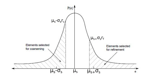
Figure 1: Statistical refinement strategy - elements in hatched areas are flagged to AMR/C process.

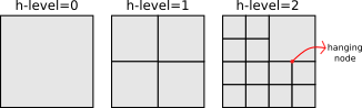
Figure 2: Adaptive mesh refinement: hierarchy of refined meshes with hanging nodes, where the solution is constrained to enforce continuity.

4 Numerical Results: Verification of the generic spatio-temporal SEIRD model

To verify the implementation of the generic spatio-temporal SEIRD model, we have done several tests. For this, we consider a square domain of $1km\times 1km$ centered at $(0,0)$ for all tests in this section.

4.1 Test 1: Reproducing a compartmental model

In the first test, we do not consider diffusion. We consider a population of 1000 $people/km^{2}$ with 1 $person/km^{2}$ initially infected in all area of the domain. Then, the initial conditions are: $s_{0}=999$, $e_{0}=0$, $i_{0}=1$, $r_{0}=0$ and $d_{0}=0$. This test aims to reproduce a compartmental simulation of the EPIDEMIC software by using the same initial parameters. The results have to be the same in each point of the domain and the same as the EPIDEMIC software. We set $\alpha=0.14286$ $days^{-1}$, $\beta=0.25$ $days^{-1}$, $\delta=0.06666$ $days^{-1}$, $\gamma=0.1$ $days^{-1}$ and $\Delta t=1$ $day$. The mesh has $50\times 50$ bilinear quadrilateral elements. Figure 3 shows the comparison of the results, where we can see a very good agreement between both solutions.

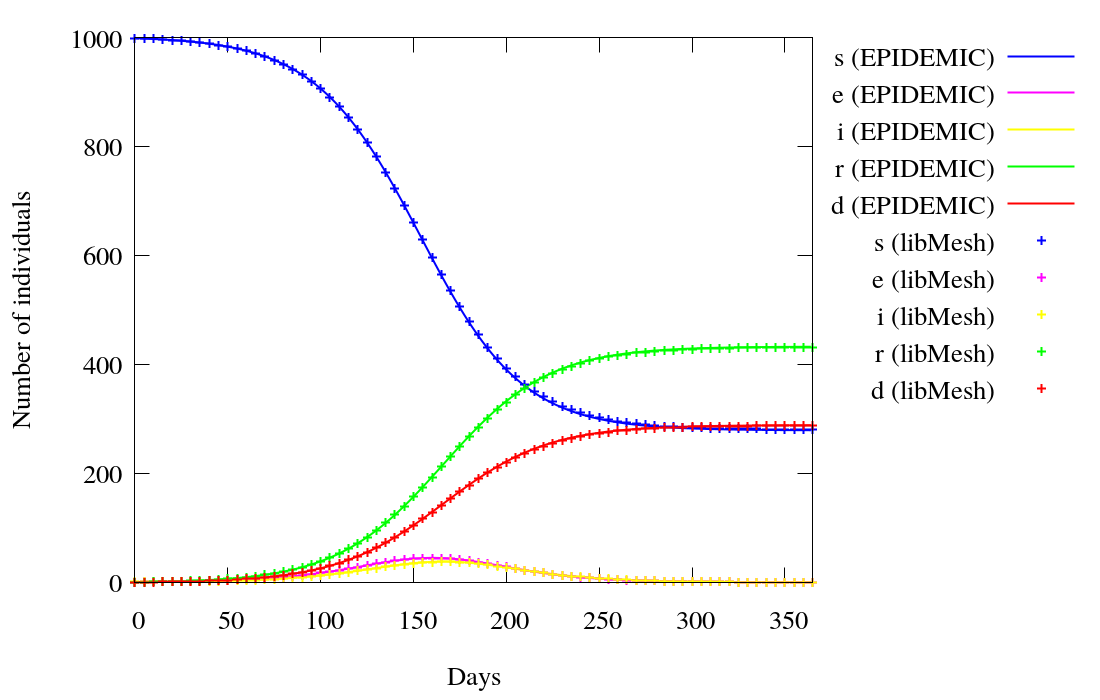
Figure 3: Test 1: Reproducing a compartmental model

Figure 4 shows the results over a centralized horizontal line crossing the domain at t=365 days. It is possible to see that the results are the same in all the domain, as expected.

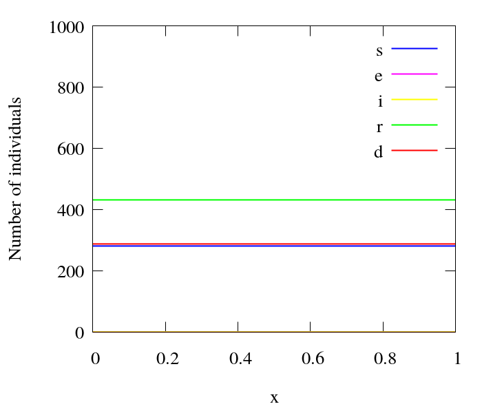
Figure 4: Test 1: Values over a centralized horizontal line at t=365 days

4.2 Test 2: Initial infected only in a circle region with diffusion

Now, we consider the same parameters of the previous example, but different initial conditions. We consider a population of 1000 $people/km^{2}$ in all area of the domain with 1 $person/km^{2}$ initially infected only in a circle centered at $(0,0)$ and radius $R=0.5$ $km$, We assume that $\nu_{s}=\nu_{e}=\nu_{i}=\nu_{r}=10^{-8}$ $km^{2}persons^{-1}days^{-1}$. Then, the initial conditions are: $s_{0}=999$, $e_{0}=0$, $i_{0}=1$ for $R<=0.5$ and $i_{0}=0$ for $R>0$ with $R=\sqrt{x^{2}+y^{2}}$, $r_{0}=0$ and $d_{0}=0$ (see Figure 5). We consider adaptive mesh refinement in this example. The original mesh has $50\times 50$ bilinear quadrilateral elements, and after the refinement, the smallest element has size 0.005 $km$. We initially refine the domain in two levels. For the AMR/C procedure, we set $h_{max}=2$,$r_{f}=0.95$, $c_{f}=0.05$. We apply the adaptive mesh refinement every 5 time-steps.

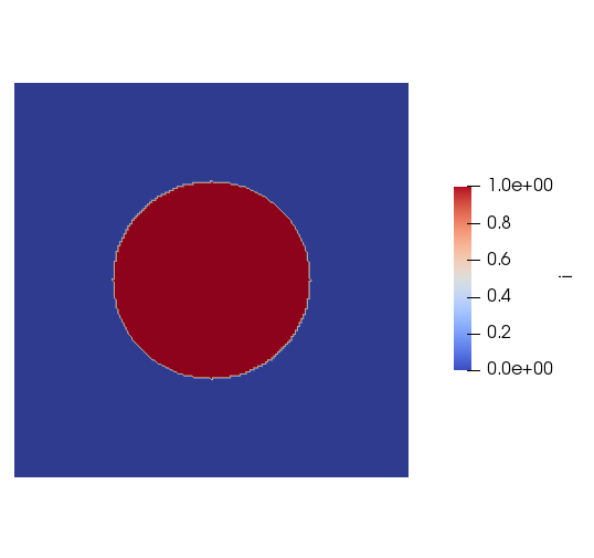
Figure 5: Test 2: Infected initial condition

Figure 6 shows the results over a centralized horizontal line crossing the domain at t=365 days. Figure 7 shows the infected people at different time-steps. Note that the infected remains actives in other parts of the domain because of the diffusion. It is possible to see the wave effect of the disease spreading. Note that the AMR/C procedure improves spatial resolution on the regions where the infected people are higher.

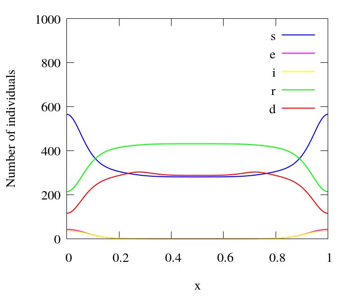
Figure 6: Test 2: Values over a centralized horizontal line at t=365 days

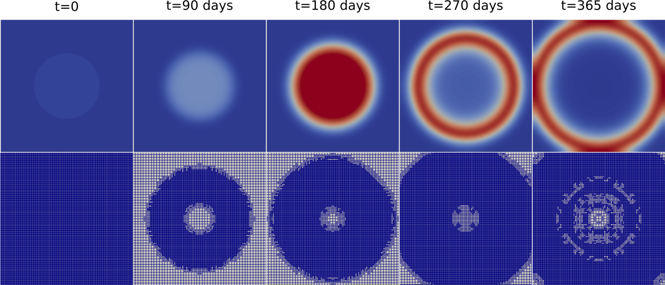
Figure 7: Test 2: Infected people at different time-steps (top) and adapted meshes (bottom).

4.3 Test 3: Varying the population

In this test, we change the initial population. Instead of a constant value in all domain, we set 1000 $people/km^{2}$ at the left/top quadrant, 500 $people/km^{2}$ at the right/top quadrant, 250 $people/km^{2}$ at the left/bottom quadrant and 750 $people/km^{2}$ at the right/bottom quadrant (Figure 8). Then, the initial conditions are: $s_{0}=999$ for $x\leq 0$ and $y>0$, $s_{0}=499$ for $x>0$ and $y>0$, $s_{0}=249$ for $x\leq 0$ and $y<=$, $s_{0}=749$ for $x>0$ and $y>0$, $e_{0}=0$, $i_{0}=1$ for $R\leq 0.5$ and $i_{0}=0$ for $R>0$ with $R=\sqrt{x^{2}+y^{2}}$, $r_{0}=0$ and $d_{0}=0$. The initial population infected is 1 $person/km^{2}$ at the same circled region of the previous test. All other parameters are the same of the previous simulation.

Figure 9 shows the infected people ate different time-steps. It is possible to see that the regions with denser populations (more $people/km^{2}$) are more affected by the disease. Figure 10 shows the total number of deaths after 365 days, and the regions with more $people/km^{2}$ have more deaths than the less dense regions. Note also that the AMR/C procedure generates meshes following the model dynamics.

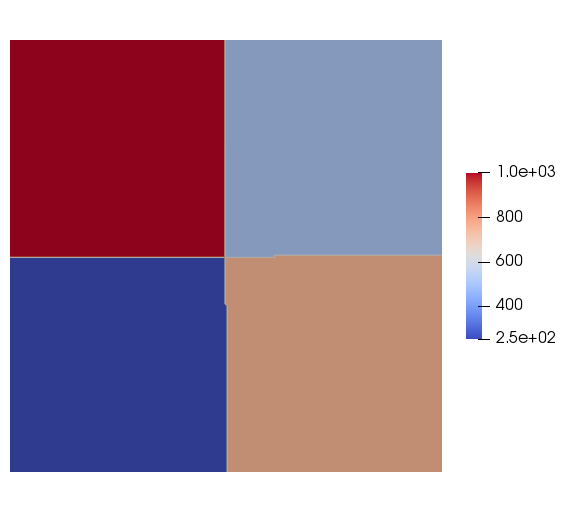
Figure 8: Test 3: Susceptible initial condition

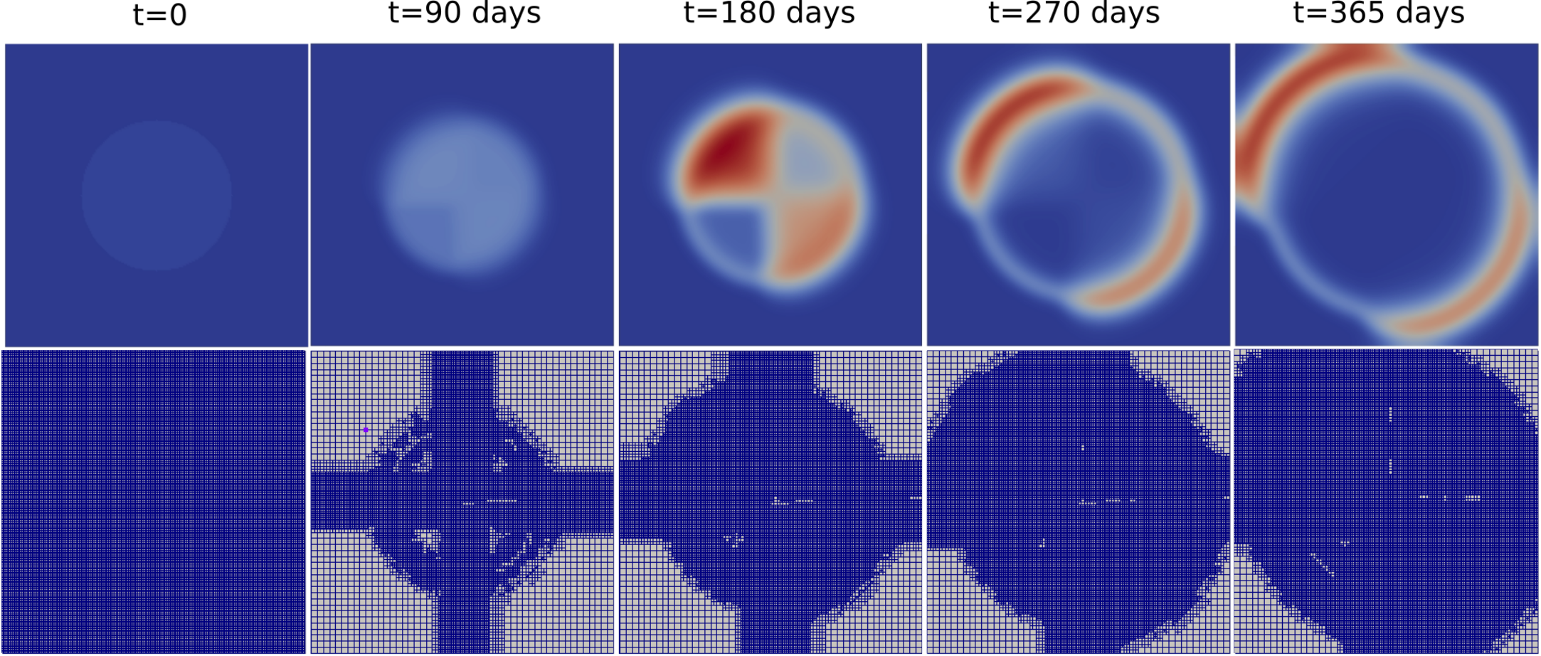
Figure 9: Test 3: Infected people at different time-steps (top) and adapted meshes (bottom).

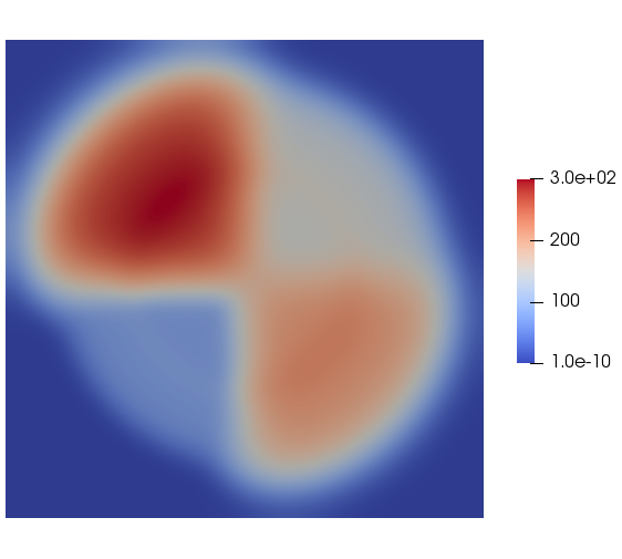
Figure 10: Test 3: Total deaths at t=365 days.

5 Numerical Results: Verification of the spatio-temporal model of COVID-19 infection spread

In this section, we perform some simulations to validate the spatio-temporal model of COVID-19 infection spread.

5.1 COVID19 Test 1: Compartmental model

In this test, we do not consider diffusion. We consider a square domain of $1km\times 1km$ centered at $(0,0)$ with a population of 1000 $people/km^{2}$, with 1 $person/km^{2}$ initially infected and 5 $people/km^{2}$ exposed in all area of the domain. Then, the initial conditions are: $s_{0}=994$, $e_{0}=5$, $i_{0}=1$, $r_{0}=0$ and $d_{0}=0$. The aim of this test is to reproduce a compartmental simulation presented in [8] by using the same initial parameters. The results has to be the same in each point of the domain and also the same of the ones given in [8]. We set $\alpha=0.125$ $days^{-1}$, $\beta_{i}=\beta_{e}=0.005$ $days^{-1}persons^{-1}$, $\delta=0.0625$ $days^{-1}$, $\gamma_{i}=0.041666667$ $days^{-1}$ and $\gamma_{e}=0.1666667$ $days^{-1}$. The mesh has $50\times 50$ bilinear quadrilateral elements. Figure 11 shows the comparison of the results, where we can see an excellent agreement.

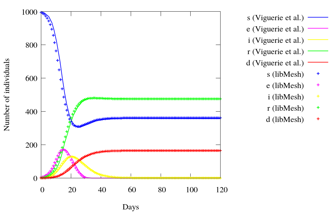
Figure 11: COVID19 Test 1: Compartmental model

5.2 COVID19 Test 2: Reproducing a 1D model

In this example, we reproduce a 1D model with quadrilateral elements being the spatial domain $\Omega$ given by $[0,1]$ and a time interval $[0,T]$ with $T=200$ days. To reproduce a 1D simulation with quadrilateral elements, we fix the element width to 0.0005 and vary its length to find the proper refinement for this case. Therefore, we run a mesh convergence study as well as a time-step convergence study.

For the initial conditions, we set $s=s_{0}$ and $e=e_{0}$ as follows,

$$s_{0}=e^{-(x+1)^{4}}+e^{-\frac{(x-0.35)^{2}}{10^{-2}}}+\frac{1}{8}\left(e^{-\frac{(x-0.62)^{4}}{10^{-5}}}+e^{-\frac{(x-0.52)^{4}}{10^{-5}}}+e^{-\frac{(x-0.42)^{4}}{10^{-5}}}\right)+\frac{1}{4}e^{-\frac{(x-0.735)^{4}}{10^{-5}}}$$ (35)

$$e_{0}=\frac{1}{20}e^{-\frac{(x-0.75)^{4}}{10^{-5}}}$$ (36)

Figure 12 shows the initial conditions. We further set $i_{0}=0$, $r_{0}=0$, and $d_{0}=0$. Qualitatively, the initial conditions represent a large population centered around $x=0.35$ with no exposed persons and a small population centered around $x=0.75$ with some exposed individuals. We also enforce homogeneous Neumann boundary conditions at $x=0$ and a zero-population Dirichlet boundary condition at $x=1$ for all model compartments. The latter represents a non-populated area at $x=1$.

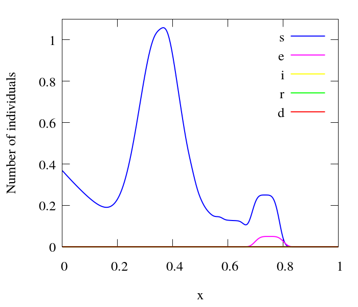
Figure 12: COVID19 Test 2: Initial conditions.

We set $\alpha=0.09375$ $days^{-1}$, $\beta_{i}=\beta_{e}=0.375$ $days^{-1}persons^{-1}$, $\delta=0.0046875$ $days^{-1}$, $\gamma_{i}=0.03125$ $days^{-1}$ and $\gamma_{e}=0.125$ $days^{-1}$, $A=0$, $\nu_{s}=3.75\times 10^{-5}$, $\nu_{e}=0.75\times 10^{-3}$, $\nu_{i}=0.75\times 10^{-10}$ and $\nu_{r}=3.75\times 10^{-5}$ $km^{2}persons^{-1}days^{-1}$.

Figure 13 shows the comparison of the results with a mesh size $\Delta x=1/500$ and a time-step $\Delta t=0.25$ $days$. For comparison, we multiply the total number of individuals by 2000, since our element width is $1/2000$ and it has influence when integrating the domain. We can observe a very good agreement between both solutions.

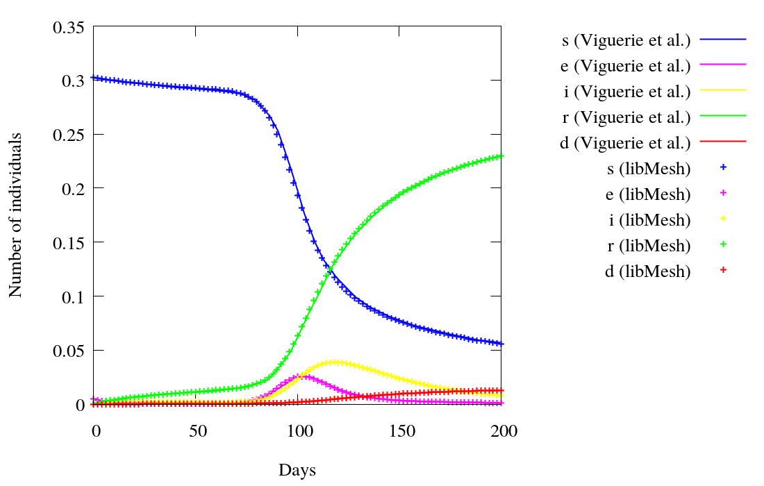
Figure 13: COVID19 Test 2: Reproducing a 1D model

Figure 14: COVID Test 2: Populations at t=200 days.

5.2.1 Mesh convergence study

We compare numerical solutions computed on successively refined uniform grids with mesh size $\Delta x=1/50,1/100,1/250,1/500$, and $1/1000$. The time step is $\Delta t=0.25$ days. Figure 15 shows the difference in the total population of each compartment of individuals for the different meshes.

A good resolution is found for $\Delta x=1/500$. It is easy to see this convergence in Figure 16, where the number of individuals of each compartment is plotted at $t=90$ days.

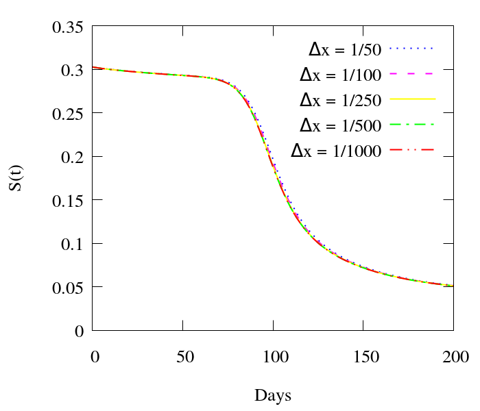
(a)

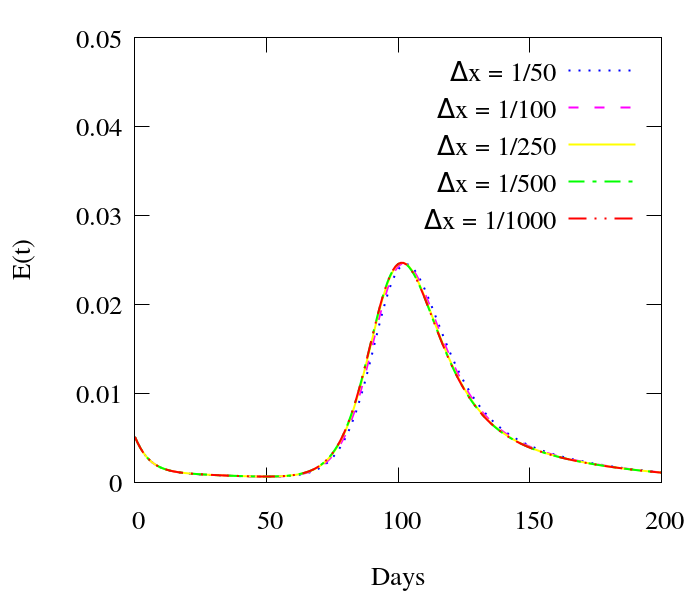
(b)

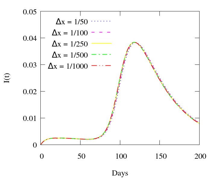
(c)

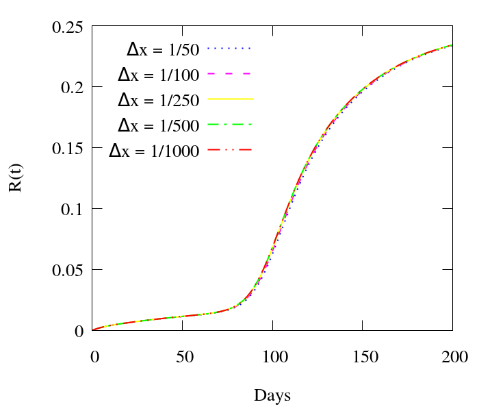
(d)

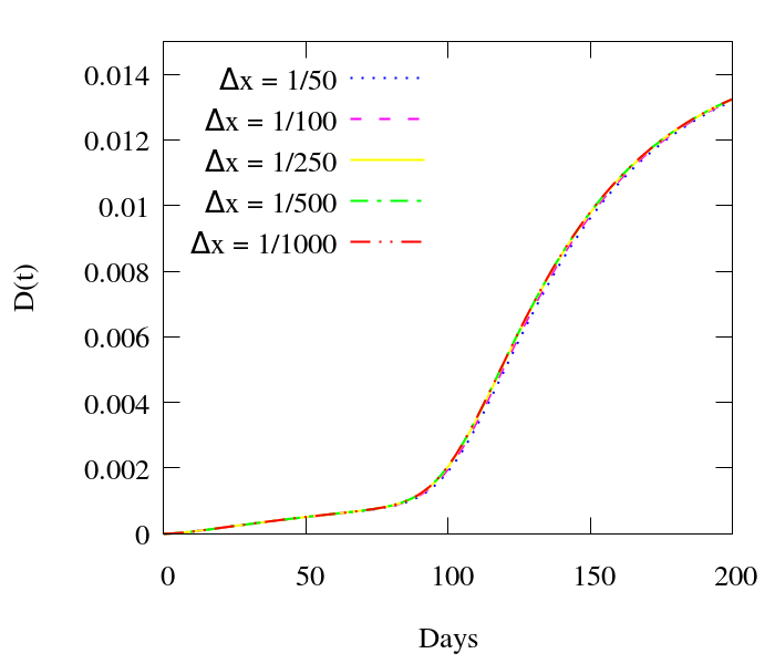
(e)

Figure 15: COVID19 Test 2: Mesh convergence study (Total population by time).

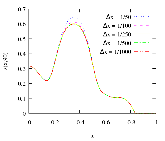
(a)

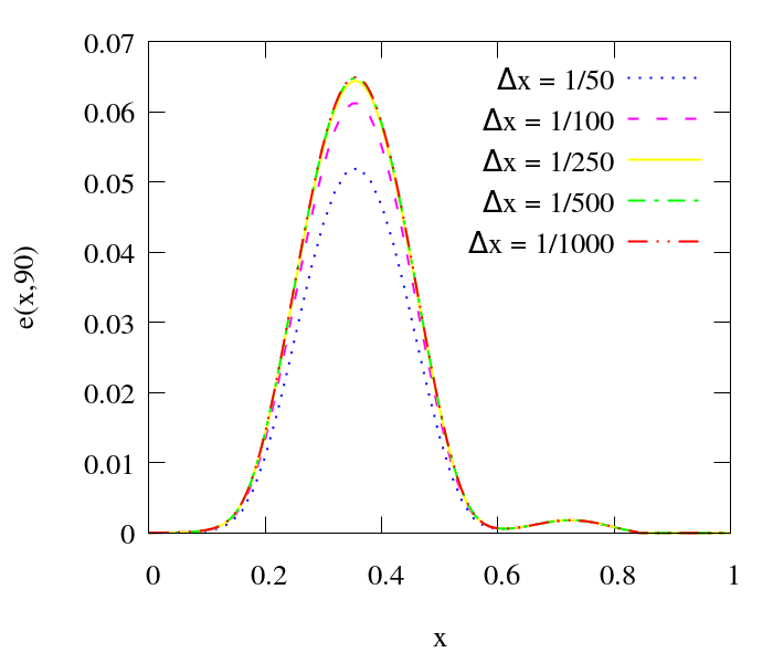
(b)

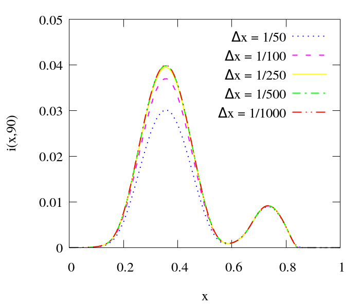
(c)

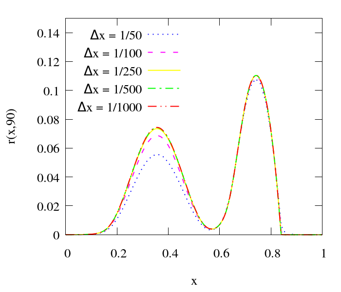
(d)

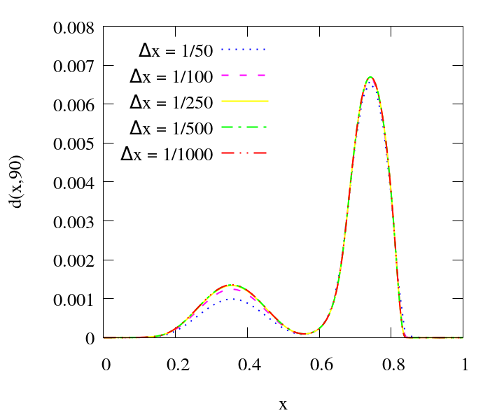
(e)

Figure 16: COVID19 Test 2: Mesh convergence study (Individuals at t=90 days).

5.2.2 Time-step convergence study

We examine the impact of time-step size $\Delta t$ on the numerical approximation of the model solution. We consider the time step sizes $\Delta t=1$, $\Delta t=0.5$, $\Delta t=0.25$, $\Delta t=0.125$ and $\Delta t=0.0625$ days. As the results in Section 5.2.1 suggested $\Delta x=1/500$ is a sufficiently fine spatial discretization, we utilize this mesh resolution here. Figure 17 shows the difference of the total population of each compartment of individuals for the different time-steps.

A good accuracy is found for $\Delta t=0.25$ days. It is easy to see how the accuracy improves in Figure 18, where the number of individuals of each compartment is plotted at $t=90$ days.

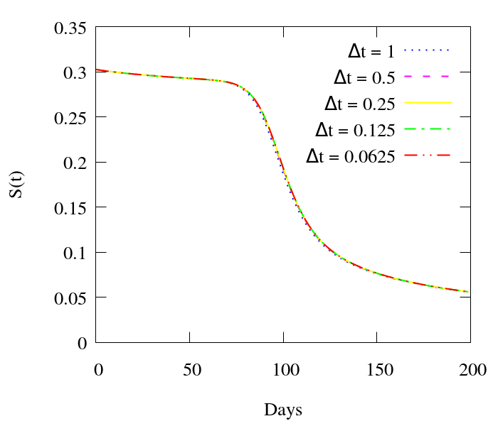
(a)

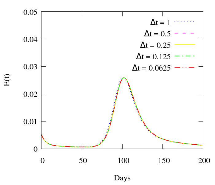
(b)

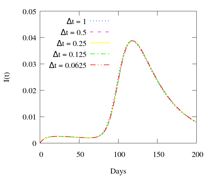
(c)

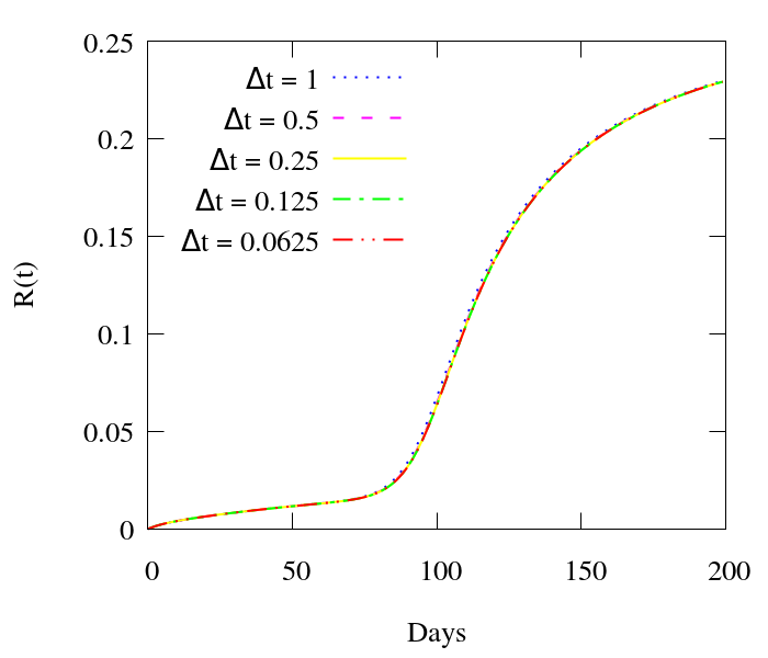
(d)

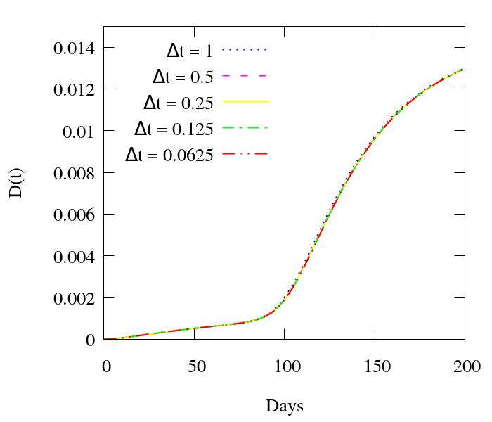
(e)

Figure 17: COVID19 Test 2: Time convergence study (Total population by time).

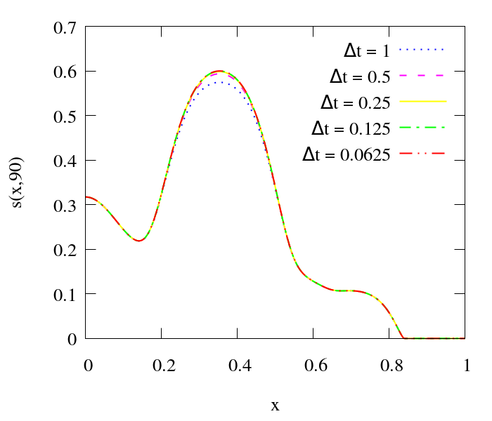
(a)

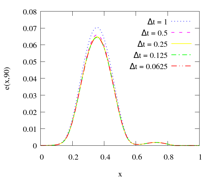
(b)

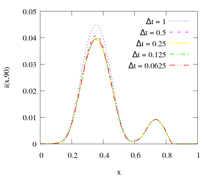
(c)

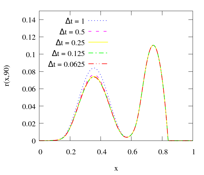
(d)

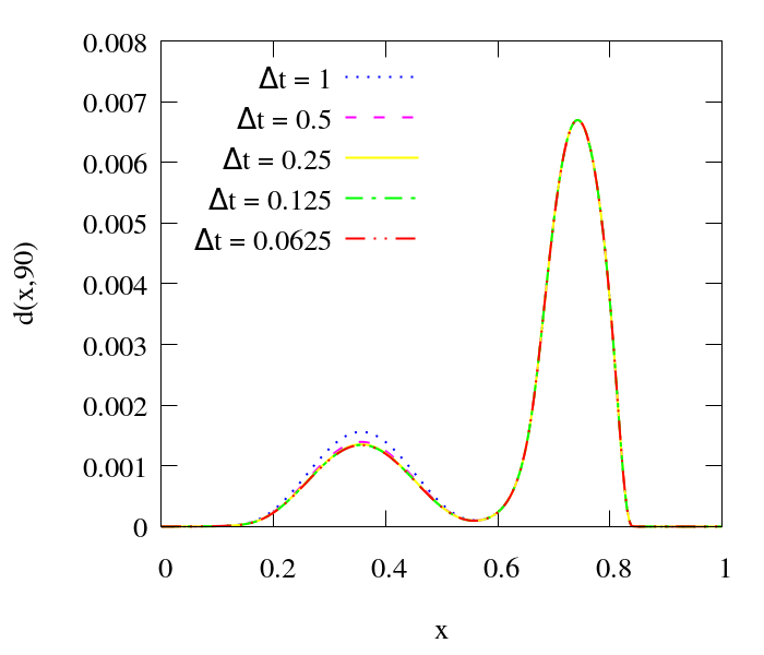
(e)

Figure 18: COVID19 Test 2: Time convergence study (Individuals at t=90 days).

5.3 COVID19 Test 3: Reproducing a 2D model

This test is the application of the previous configuration rotated in a two dimensional square with corners at (-1,-1), (1,-1), (1,1) and (-1,1). The initial population is:

$$s_{0}=e^{-(R+1)^{4}}+e^{-\frac{(R-0.35)^{2}}{10^{-2}}}+\frac{1}{8}\left(e^{-\frac{(R-0.62)^{4}}{10^{-5}}}+e^{-\frac{(R-0.52)^{4}}{10^{-5}}}+e^{-\frac{(R-0.42)^{4}}{10^{-5}}}\right)+\frac{1}{4}e^{-\frac{(R-0.735)^{4}}{10^{-5}}}$$ (37)

$$e_{0}=\frac{1}{20}e^{-\frac{(R-0.75)^{4}}{10^{-5}}}$$ (38)

with $R=\sqrt{x^{2}+y^{2}}$.

The original mesh has $50\times 50$ bilinear quadrilaterals elements and it is refined in two levels at the beginning of the simulation. For the AMR/C procedure, we set $h_{max}=2$, $r_{f}=0.95$, $c_{f}=0.05$. We apply the adaptive mesh refinement every 4 time-steps. The behavior of the transmission has to be similar to the 1D model results, but in a radial configuration. Figures 19 shows the populations at different time steps. Figure 6 shows the results over a centralized horizontal line (or vertical because the axisymmetry) crossing the domain at t=200 days. If we compare Figure 6 with Figure 14, it is possible to see that the populations follow a similar behavior.

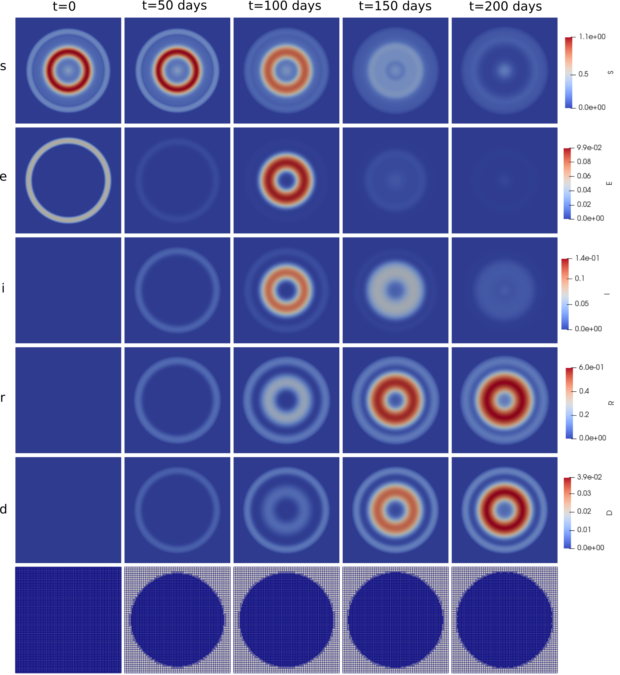
Figure 19: COVID Test 3: Populations at different times (top rows) and adapted meshes (bottom).

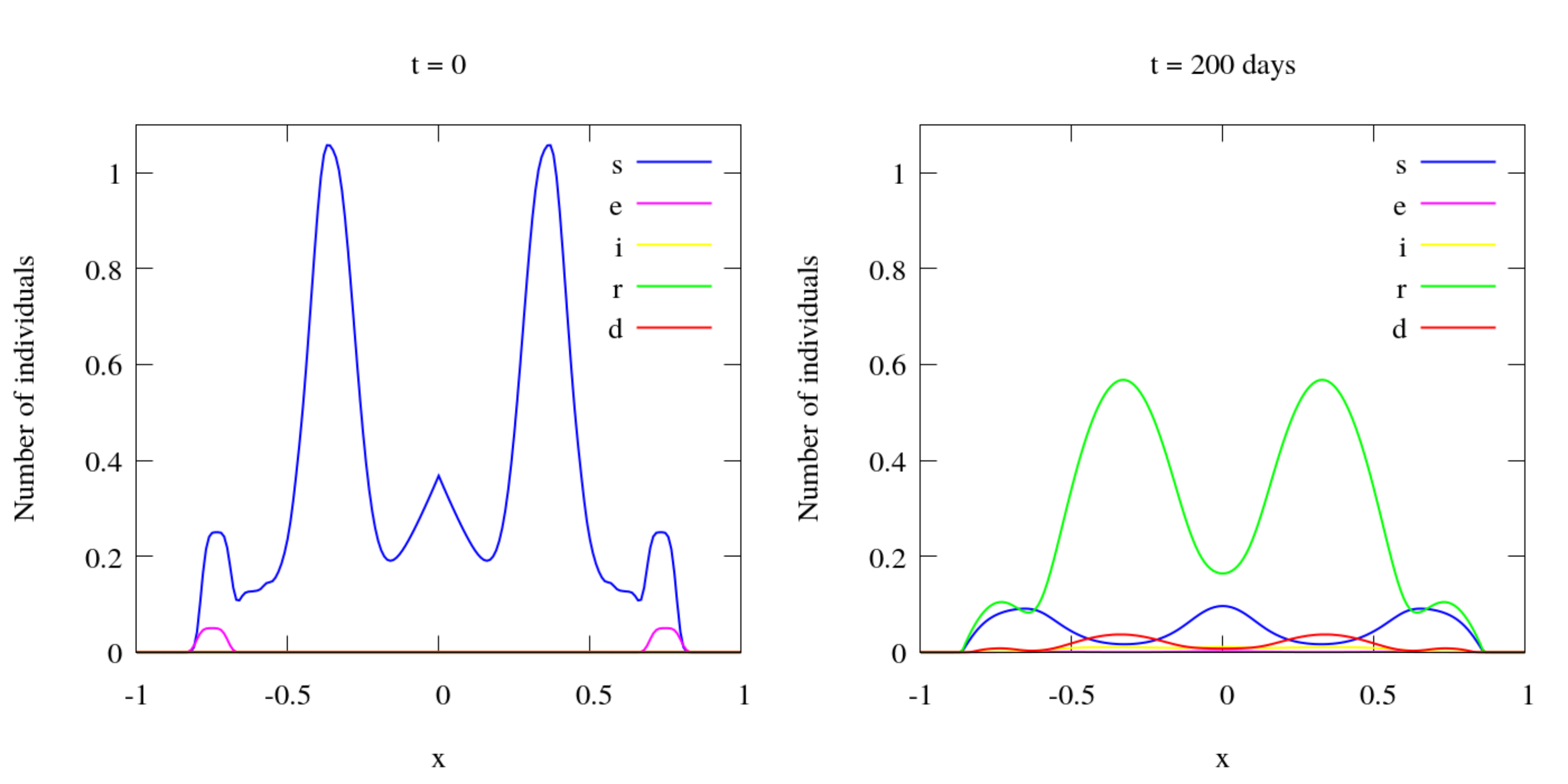
Figure 20: COVID Test 3: Populations over a horizontal/vertical line crossing the middle of the domain.

In Figure 21 we plot the time history of the total number of individuals. There is a small gain in the total number of individuals (less than 0.1%).

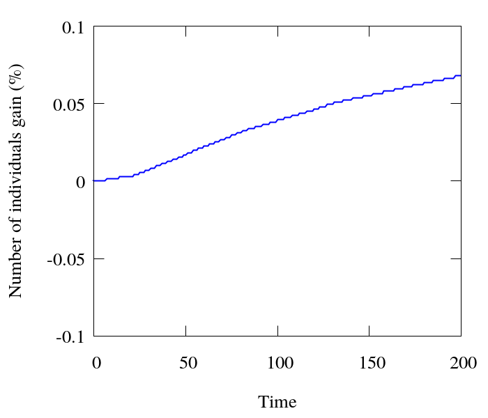
Figure 21: COVID Test 3: Time history of the total number of individuals.

5.4 COVID19 Test 4: Anisotropic diffusion

This test considers anisotropic diffusion in the previous configuration (only in the $x$ direction). Therefore, the populations move spatially only in the $x$ direction. Figure 22 shows the populations at different time-steps. Figure 23 shows the results over a centralized horizontal line crossing the domain, and Figure 24 over a centralized vertical line. By comparing these two figures, it is clear how the diffusion direction influences the behavior of the virus spread. Since there is no movement of infected or exposed people in the $y$ direction, part of the population does not have contact with the virus because there is no chance of the virus to reach them.

In Figure 25 we plot the time history of the total number of individuals. We can see a gain in the total number of individuals of less than 0.1%.

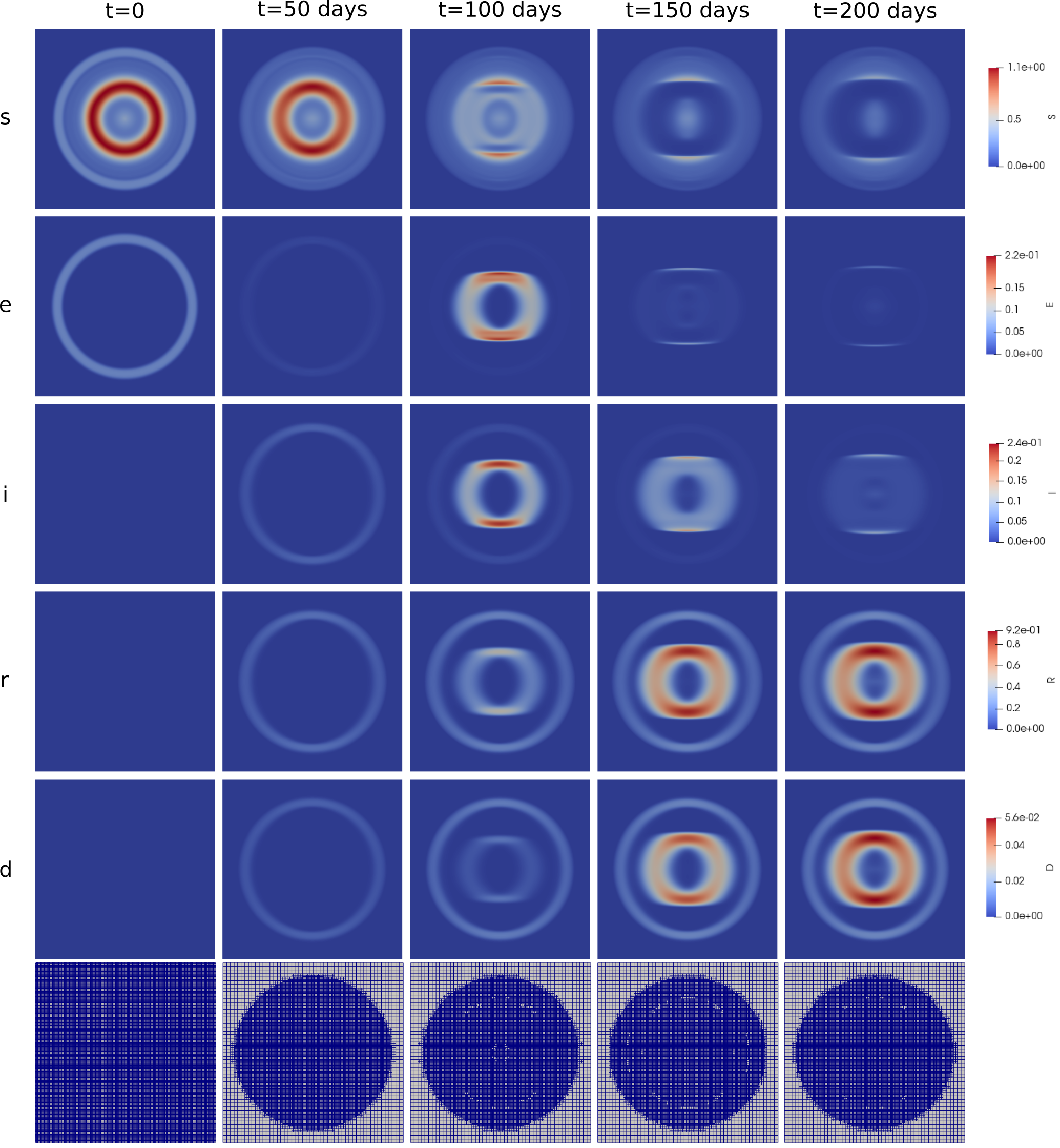
Figure 22: COVID Test 4: Populations at different times (top rows) and adapted meshes (bottom)

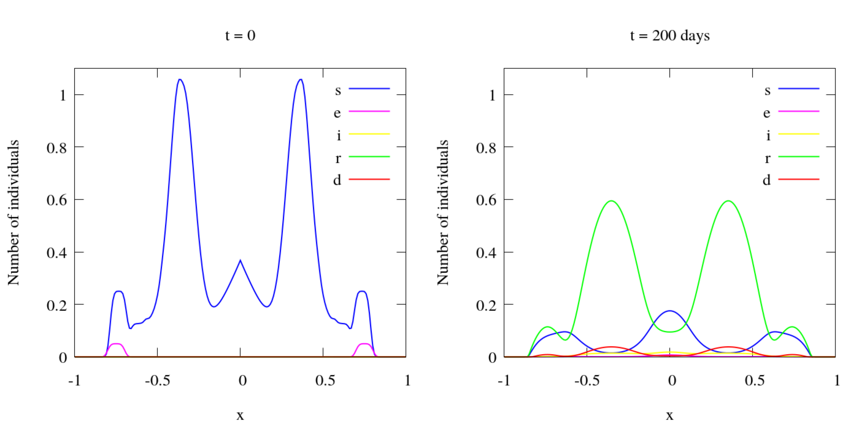
Figure 23: COVID Test 4: Populations over a horizontal line crossing the middle of the domain.

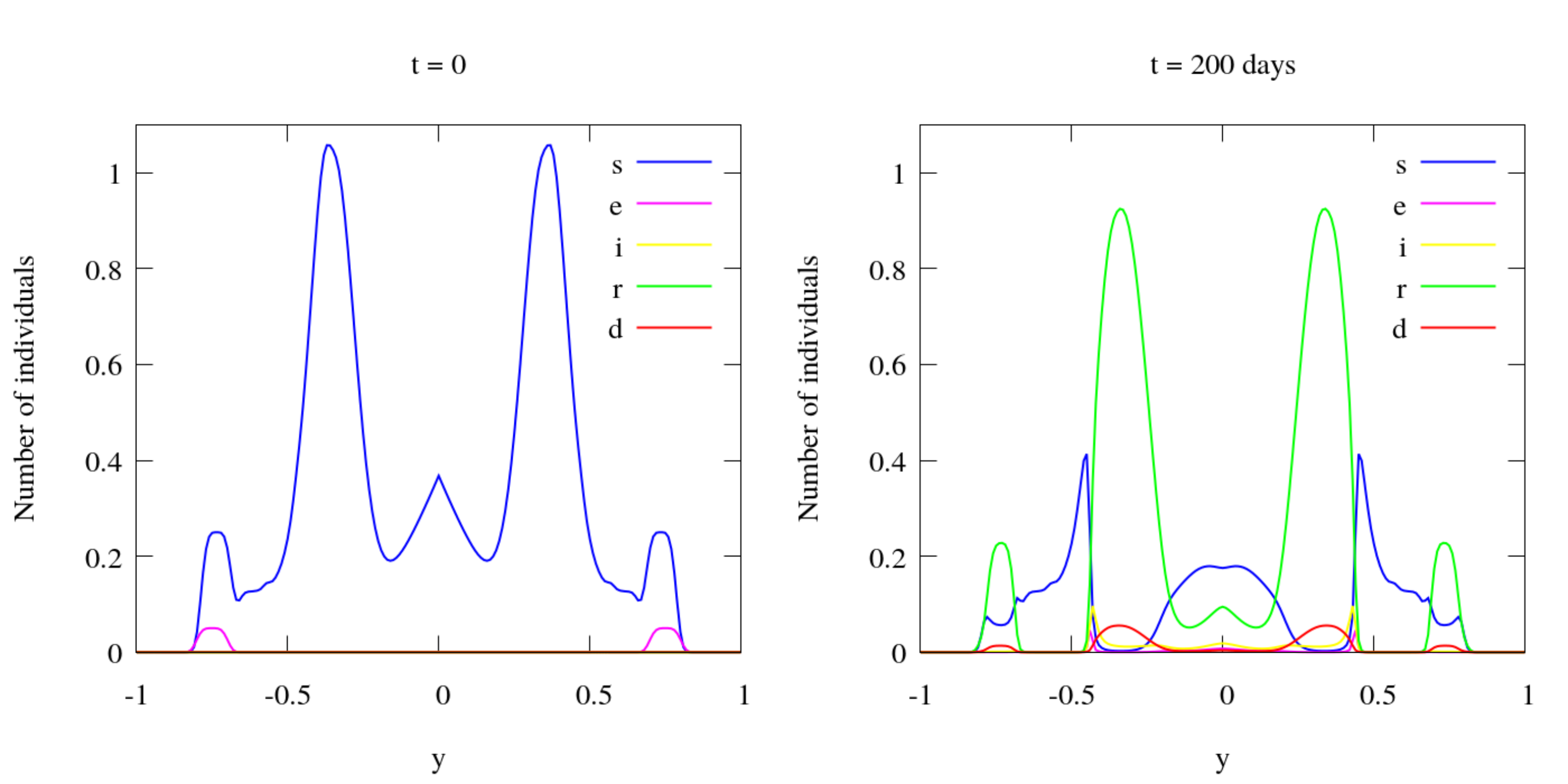
Figure 24: COVID Test 4: Populations over a vertical line crossing the middle of the domain.

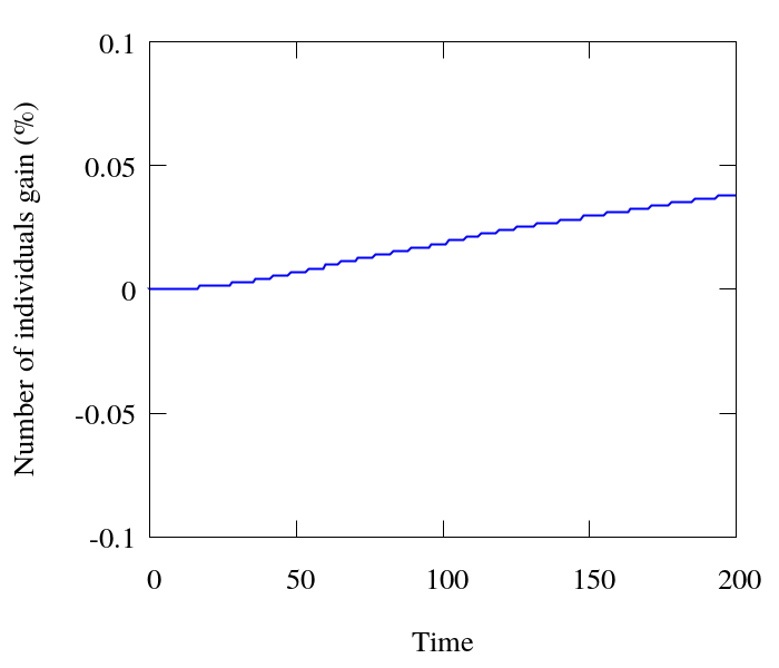
Figure 25: COVID Test 4: Time history of the total number of individuals.

5.5 COVID19 Test 5: Random source

This test has a new configuration. We still work with the two dimensional square with corners at (-1,-1), (1,-1), (1,1) and (-1,1) and an anisotropic diffusion only in the $x$ direction. We set $\alpha=0.09375$ $days^{-1}$, $\beta_{i}=\beta_{e}=0.375/n$ $days^{-1}persons^{-1}$, $\delta=0.0046875$ $days^{-1}$, $\gamma_{i}=0.03125$ $days^{-1}$ and $\gamma_{e}=0.125$ $days^{-1}$, $A=0$, $\nu_{s}=3.75\times 10^{-9}$, $\nu_{e}=0.75\times 10^{-7}$, $\nu_{i}=0.75\times 10^{-14}$ and $\nu_{r}=3.75\times 10^{-9}$ $km^{2}persons^{-1}days^{-1}$, and $\Delta t=0.25$ $days$.

The original mesh has $50\times 50$ bilinear quadrilaterals elements and it is refined in two levels at the beginning of the simulation. For the AMR/C procedure, we set $h_{max}=2$, $r_{f}=0.95$, $c_{f}=0.05$. We apply the adaptive mesh refinement every 4 time-steps.

The initial population is:

$$\begin{split}s_{0}=max\left\{\begin{array}[]{ccc}100000e^{-\frac{R_{1}^{4}}{10^{-2}}}\\ 10000e^{-\frac{R_{2}^{4}}{10^{-4}}}\\ 10000e^{-\frac{R_{3}^{4}}{10^{-4}}}\\ 1000\end{array}\right.\end{split}$$ (39)

$$e_{0}=0$$ (40)

$$i_{0}=0$$ (41)

$$R_{1}=\sqrt{x^{2}+y^{2}}$$ (42)

$$R_{2}=\sqrt{x^{2}+(y-0.75)^{2}}$$ (43)

$$R_{3}=\sqrt{(x-0.75)^{2}+y^{2}}$$ (44)

Figure 26 shows the initial susceptible population. Note there are not infected or exposed people at the initial time. We implement a random source of the exposed population that depends on the number of susceptible people. In all time-steps random nodes of the domain receive a certain number of exposed people. It tries to simulate people who travel and suddenly appear in a region carrying the virus. The random source does not add individuals to the population, but change individuals between susceptible and exposed compartments. Of course, this model is simple. Nevertheless, it demonstrates how to handle a random source term in the equations. Figure 27 shows a example of the random exposed number of people that appears in one time-step.

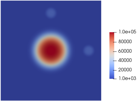
Figure 26: COVID Test 5: Initial susceptible population.

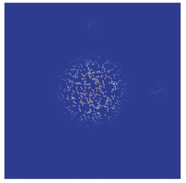
Figure 27: COVID Test 5: Example of the random source of exposed people.

Figure 28 shows the populations at different time-steps. We see oscillations in the number of individuals of the populations coming from the random source dynamic. These oscillations are smoothed in the $x$ direction because of the diffusion. We can see this better in Figures 29 and 30 that shows the results over a centralized horizontal and vertical line crossing the domain, respectively. The vertical plot shows unsmoothed oscillations coming from the random source in the $y$ direction. In this example, it is possible to better seeing the effects of anisotropic diffusion. Note that in the horizontal plot, the populations spread over the $x$ direction, while in the vertical plot, the populations change the compartments but stay in the same coordinates.

In Figure 31, we plot the time history of the total number of individuals. There is a negligible increase in the total number of individuals (less than 0.1%).

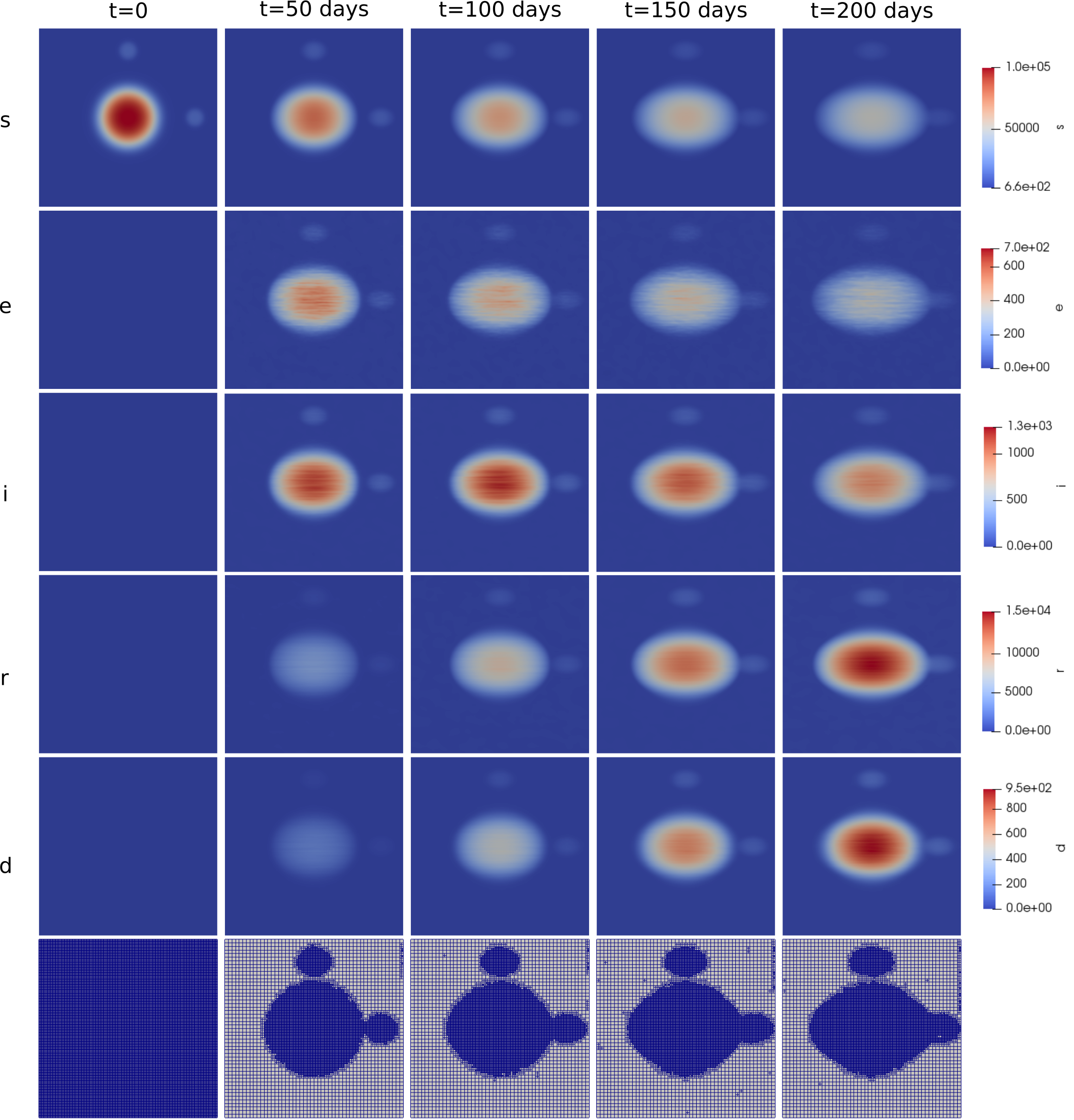
Figure 28: COVID Test 5: Populations at different times (top rows) and adapted meshes (bottom).

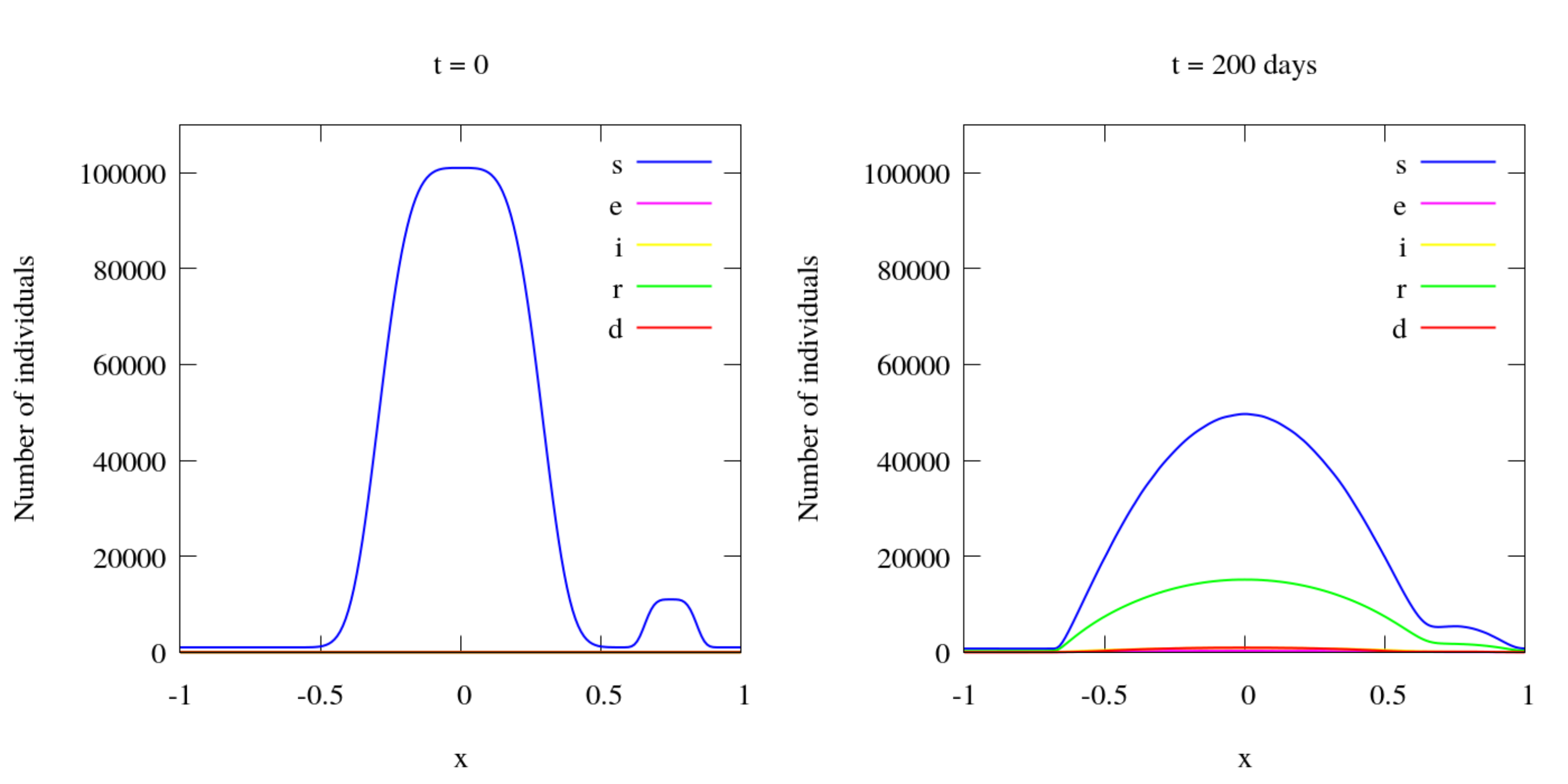
Figure 29: COVID Test 5: Populations over a horizontal line crossing the middle of the domain.

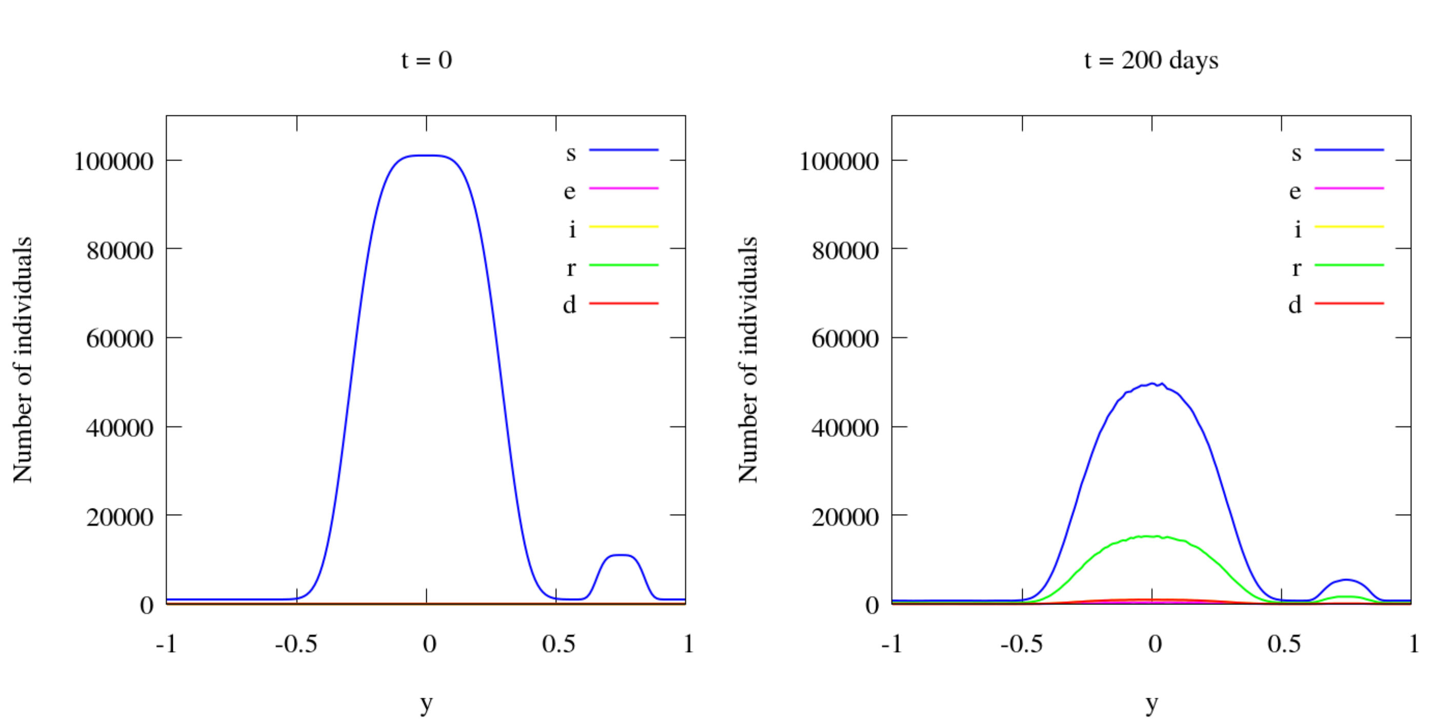
Figure 30: COVID Test 5: Populations over a vertical line crossing the middle of the domain.

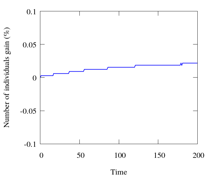
Figure 31: COVID Test 5: Time history of the total number of individuals.

6 Conclusions

We developed an extended continuum SEIRD model to represent the dynamics of the COVID-19 virus spread based on the framework proposed in [9]. We validate our code by comparing our results with other simulations. We introduce new test cases to highlight new modeling capabilities. Among the new features added to the base model, there is the addition of a source term, which represents exposed people who return from travel, by changing individuals from the susceptible compartment to the exposed compartment. We also add the possibility of anisotropic non-homogeneous diffusion. Our code is implemented through the libMesh library and supports adaptive mesh refinement and coarsening. Therefore, it can represent several spatial scales, adapting the resolution to the disease dynamics.

Data is essential to define the epidemic spreading parameters, as diffusion and infection rate. We have to study how it would be the best way to represent people who return from travels, addressing questions like defining the probability of a random source appearing in the system, in which area, the population density, among others. Diffusion-reaction models, as the present one, are richer than standard compartmental models. However, they are slower, which hampers their widespread utilization in what-if scenarios, parametric studies, and time-critical situations. Therefore, the development of low-dimensional computational models will leverage the ability of continuous models to perform in real-time scenarios. Projection-based or data-driven model order reduction [42, 43] aims to lower the computational complexity of a given computational model by reducing its dimensionality (or order), can provide this leverage. They can work in conjunction with emerging machine learning methods such as physics informed neural networks [44]. We can foresee a tremendous impact in the mathematical epidemiology field of all these new methods and techniques, enlarging the predictive capabilities and computational efficiency of diffusion-reaction epidemiological models.

Appendix A Implementation of the generic spatio-temporal SEIRD model

We implement the generic SEIRD model similar to the EPIDEMIC software. We have used the BDF2 time discretization method, Newton’s method for the nonlinear terms, and we simplify the number of the living population by considering the previous time-step solution. For all test cases the nonlinear tolerance for Newton’s method is set to $10^{-8}$ and the linear solver tolerance is set to $10^{-10}$. The linear solver is GMRES with ILU(0) preconditioner.

In libMesh, we calculate directly the new solution ($\mathbf{u}_{n+1})$ instead of the variation ($\delta\mathbf{u})$. Then, on the left-hand side, we gather the terms containing an unknown, whereas all the other terms are taken to the right-hand-side. The superscript $k$ is from the previous Newton iteration. The terms in black are from the mass matrix, in blue are the nonlinear terms, in red the diffusive terms, and in green the remaining terms from the stiffness matrix. The finite element shape functions are represented by $N_{a}$, $a=1,\cdots,n_{nnos}$, where $n_{nnos}$ is the number of nodes in the finite element mesh.

Susceptible (Equation 5):

$$K_{ss}=\int_{\Omega_{e}}1.5N_{a}N_{b}d\Omega{\color[rgb]{0,0,1}+\Delta t\int_{\Omega_{e}}N_{a}\beta N_{b}\frac{i_{k}}{n_{k}}}{\color[rgb]{1,0,0}+\Delta t\int_{\Omega_{e}}\nabla N_{a}n_{k}\nu_{s}\nabla N_{b}d\Omega}$$ (45)

$$K_{si}={\color[rgb]{0,0,1}\Delta t\int_{\Omega_{e}}N_{a}\beta N_{b}\frac{s_{k}}{n_{k}}d\Omega}$$ (46)

$$F_{s}=\int_{\Omega_{e}}N_{a}(2s_{n}-0.5s_{n-1})d\Omega{\color[rgb]{0,0,1}+\Delta t\int_{\Omega_{e}}N_{a}\beta\frac{s_{k}i_{k}}{n_{k}}d\Omega}$$ (47)

Exposed (Equation 6):

$$K_{ee}=\int_{\Omega_{e}}1.5N_{a}N_{b}d\Omega{\color[rgb]{0,1,0}+\Delta t\int_{\Omega_{e}}\alpha N_{a}N_{b}d\Omega}{\color[rgb]{1,0,0}+\Delta t\int_{\Omega_{e}}\nabla N_{a}n_{old}\nu_{e}\nabla N_{b}d\Omega}$$ (48)

$$K_{ei}={\color[rgb]{0,0,1}-\Delta t\int_{\Omega_{e}}N_{a}\beta N_{b}\frac{s_{k}}{n_{k}}d\Omega}$$ (49)

$$K_{es}={\color[rgb]{0,0,1}-\Delta t\int_{\Omega_{e}}N_{a}\beta N_{b}\frac{i_{k}}{n_{k}}d\Omega}$$ (50)

$$F_{e}=\int_{\Omega_{e}}N_{a}(2e_{n}-0.5e_{n-1})d\Omega{\color[rgb]{0,0,1}-\Delta t\int_{\Omega_{e}}N_{a}\beta\frac{s_{k}i_{k}}{n_{k}}d\Omega}$$ (51)

Infected (Equation 7):

$$K_{ii}=\int_{\Omega_{e}}1.5N_{a}N_{b}d\Omega{\color[rgb]{0,1,0}+\Delta t\int_{\Omega_{e}}(\gamma+\delta)N_{a}N_{b}d\Omega}{\color[rgb]{1,0,0}+\Delta t\int_{\Omega_{e}}\nabla N_{a}n_{k}\nu_{i}\nabla N_{b}d\Omega}$$ (52)

$$K_{ie}={\color[rgb]{0,1,0}-\Delta t\int_{\Omega_{e}}\alpha N_{a}N_{b}d\Omega}$$ (53)

$$F_{i}=\int_{\Omega_{e}}N_{a}(2i_{n}-0.5i_{n-1})d\Omega$$ (54)

Recovered (Equation 8):

$$K_{rr}=\int_{\Omega_{e}}1.5N_{a}N_{b}d\Omega{\color[rgb]{1,0,0}+\Delta t\int_{\Omega_{e}}\nabla N_{a}n_{k}\nu_{r}\nabla N_{b}d\Omega}$$ (55)

$$K_{ri}={\color[rgb]{0,1,0}-\Delta t\int_{\Omega_{e}}\gamma N_{a}N_{b}d\Omega}$$ (56)

$$F_{r}=\int_{\Omega_{e}}N_{a}(2r_{n}-0.5r_{n-1})d\Omega$$ (57)

Diseased (Equation 9):

$$K_{dd}=\int_{\Omega_{e}}1.5N_{a}N_{b}d\Omega$$ (58)

$$K_{di}={\color[rgb]{0,1,0}-\Delta t\int_{\Omega_{e}}\delta N_{a}N_{b}d\Omega}$$ (59)

$$F_{d}=\int_{\Omega_{e}}N_{a}(2d_{n}-0.5d_{n-1})d\Omega$$ (60)

Appendix B Implementation of the spatio-temporal model of COVID-19 infection spread

We present the matrix contributions of the system of equations that represents the COVID19 dynamics [9, 8]. We use the BDF2 time discretization method, Newton’s method for the nonlinear terms, and we simplify the number of the living population by considering the previous linear solution. For all test cases the nonlinear tolerance for Newton’s method is set to $10^{-8}$ and the linear solver tolerance is set to $10^{-10}$. The linear solver is GMRES with ILU(0) preconditioner.

In libMesh, we calculate directly the new solution ($\mathbf{u}_{n+1})$ instead of the variation ($\delta\mathbf{u})$. Then, on the left-hand side, we gather the terms containing an unknown, whereas all the other terms are taken to the right-hand-side. The superscript $k$ is from the previous Newton iteration. The terms in black are from the mass matrix, in blue are the nonlinear terms, in red the diffusive terms, in green the remaining terms from the stiffness matrix and in yellow the source terms.

Susceptible (Equation 15):

$$\begin{split}K_{ss}=\int_{\Omega_{e}}1.5N_{a}N_{b}d\Omega{\color[rgb]{0,0,1}+\Delta t\int_{\Omega_{e}}N_{a}\beta_{i}\left(1-\frac{A}{n_{k}}\right)N_{b}i_{k}+\Delta t\int_{\Omega_{e}}N_{a}\beta_{e}\left(1-\frac{A}{n_{k}}\right)N_{b}e_{k}d\Omega}\\ {\color[rgb]{1,0,0}+\Delta t\int_{\Omega_{e}}\nabla N_{a}n_{k}\nu_{s}\nabla N_{b}d\Omega}\end{split}$$ (61)

$$K_{si}={\color[rgb]{0,0,1}\Delta t\int_{\Omega_{e}}N_{a}\beta_{i}\left(1-\frac{A}{n_{k}}\right)N_{b}s_{k}d\Omega}$$ (62)

$$K_{se}={\color[rgb]{0,0,1}\Delta t\int_{\Omega_{e}}N_{a}\beta_{e}\left(1-\frac{A}{n_{k}}\right)N_{b}s_{k}d\Omega}$$ (63)

$$\begin{split}F_{s}=\int_{\Omega_{e}}N_{a}(2s_{n}-0.5s_{n-1})d\Omega{\color[rgb]{0,0,1}+\Delta t\int_{\Omega_{e}}N_{a}\beta_{i}\left(1-\frac{A}{n_{k}}\right)s_{k}i_{k}d\Omega+\Delta t\int_{\Omega_{e}}N_{a}\beta_{e}\left(1-\frac{A}{n_{k}}\right)s_{k}e_{k}d\Omega}{\color[rgb]{1,1,0}+f}\end{split}$$ (64)

Exposed (Equation 16):

$$\begin{split}K_{ee}=\int_{\Omega_{e}}1.5N_{a}N_{b}d\Omega{\color[rgb]{0,1,0}+\Delta t\int_{\Omega_{e}}(\alpha+\gamma_{e})N_{a}N_{b}d\Omega}{\color[rgb]{1,0,0}+\Delta t\int_{\Omega_{e}}\nabla N_{a}n_{k}\nu_{e}\nabla N_{b}d\Omega}\\ {\color[rgb]{0,0,1}-\Delta t\int_{\Omega_{e}}N_{a}\beta_{e}\left(1-\frac{A}{n_{k}}\right)N_{b}s_{k}d\Omega}\end{split}$$ (65)

$$K_{ei}={\color[rgb]{0,0,1}-\Delta t\int_{\Omega_{e}}N_{a}\beta_{i}\left(1-\frac{A}{n_{k}}\right)N_{b}s_{k}d\Omega}$$ (66)

$$K_{es}={\color[rgb]{0,0,1}-\Delta t\int_{\Omega_{e}}N_{a}\beta_{i}\left(1-\frac{A}{n_{k}}\right)N_{b}i_{k}d\Omega-\Delta t\int_{\Omega_{e}}N_{a}\beta_{e}\left(1-\frac{A}{n_{k}}\right)N_{b}e_{k}d\Omega}$$ (67)

$$\begin{split}F_{e}=\int_{\Omega_{e}}N_{a}(2e_{n}-0.5e_{n-1})d\Omega{\color[rgb]{0,0,1}-\Delta t\int_{\Omega_{e}}N_{a}\beta_{i}\left(1-\frac{A}{n_{k}}\right)s_{k}i_{k}d\Omega}\\ {\color[rgb]{0,0,1}-\Delta t\int_{\Omega_{e}}N_{a}\beta_{e}\left(1-\frac{A}{n_{k}}\right)s_{k}e_{k}d\Omega}{\color[rgb]{1,1,0}-f}\end{split}$$ (68)

Infected (Equation 17):

$$K_{ii}=\int_{\Omega_{e}}1.5N_{a}N_{b}d\Omega{\color[rgb]{0,1,0}+\Delta t\int_{\Omega_{e}}(\gamma_{i}+\delta)N_{a}N_{b}d\Omega}{\color[rgb]{1,0,0}+\Delta t\int_{\Omega_{e}}\nabla N_{a}n_{k}\nu_{i}\nabla N_{b}d\Omega}$$ (69)

$$K_{ie}={\color[rgb]{0,1,0}-\Delta t\int_{\Omega_{e}}\alpha N_{a}N_{b}d\Omega}$$ (70)

$$F_{i}=\int_{\Omega_{e}}N_{a}(2i_{n}-0.5i_{n-1})d\Omega$$ (71)

Recovered (Equation 18):

$$K_{rr}=\int_{\Omega_{e}}1.5N_{a}N_{b}d\Omega{\color[rgb]{1,0,0}+\Delta t\int_{\Omega_{e}}\nabla N_{a}n_{k}\nu_{r}\nabla N_{b}d\Omega}$$ (72)

$$K_{ri}={\color[rgb]{0,1,0}-\Delta t\int_{\Omega_{e}}\gamma_{i}N_{a}N_{b}d\Omega}$$ (73)

$$K_{re}={\color[rgb]{0,1,0}-\Delta t\int_{\Omega_{e}}\gamma_{e}N_{a}N_{b}d\Omega}$$ (74)

$$F_{r}=\int_{\Omega_{e}}N_{a}(2r_{n}-0.5r_{n-1})d\Omega$$ (75)

Diseased (Equation 19):

$$K_{dd}=\int_{\Omega_{e}}1.5N_{a}N_{b}d\Omega$$ (76)

$$K_{di}={\color[rgb]{0,1,0}-\Delta t\int_{\Omega_{e}}\delta N_{a}N_{b}d\Omega}$$ (77)

$$F_{d}=\int_{\Omega_{e}}N_{a}(2d_{n}-0.5d_{n-1})d\Omega$$ (78)

References

- [1] Hyun Mo Yang. Epidemiologia matemática: Estudos dos efeitos da vacinação em doenças de transmissão direta. Editora da UNICAMP, 2001.
- [2] Richard A Erickson, Steven M Presley, Linda JS Allen, Kevin R Long, and Stephen B Cox. A dengue model with a dynamic aedes albopictus vector population. Ecological Modelling, 221(24):2899–2908, 2010.
- [3] Eber Dantas, Michel Tosin, and Americo Cunha Jr. Calibration of a seir–sei epidemic model to describe the zika virus outbreak in brazil. Applied Mathematics and Computation, 338:249–259, 2018.
- [4] Zindoga Mukandavire, Prasenjit Das, Christinah Chiyaka, and Farai Nyabadza. Global analysis of an hiv/aids epidemic model. World Journal of Modelling and Simulation, 6(3):231–240, 2010.
- [5] Chris Dye and Nigel Gay. Modeling the sars epidemic. Science, 300(5627):1884–1885, 2003.
- [6] Alemayehu Midekisa, Gabriel Senay, Geoffrey M Henebry, Paulos Semuniguse, and Michael C Wimberly. Remote sensing-based time series models for malaria early warning in the highlands of ethiopia. Malaria Journal, 11(1):165, 2012.
- [7] Phenyo E Lekone and Bärbel F Finkenstädt. Statistical inference in a stochastic epidemic seir model with control intervention: Ebola as a case study. Biometrics, 62(4):1170–1177, 2006.
- [8] Alex Viguerie, Alessandro Veneziani, Guillermo Lorenzo, Davide Baroli, Nicole Aretz-Nellesen, Alessia Patton, Thomas E Yankeelov, Alessandro Reali, Thomas JR Hughes, and Ferdinando Auricchio. Diffusion–reaction compartmental models formulated in a continuum mechanics framework: application to covid-19, mathematical analysis, and numerical study. Computational Mechanics, pages 1–22, 2020.
- [9] Alex Viguerie, Guillermo Lorenzo, Ferdinando Auricchio, Davide Baroli, Thomas JR Hughes, Alessia Patton, Alessandro Reali, Thomas E Yankeelov, and Alessandro Veneziani. Simulating the spread of covid-19 via spatially-resolved susceptible-exposed-infected-recovered-deceased (seird) model with heterogeneous diffusion. Applied Mathematics Letters, 111:106617, 2021.
- [10] Julien Arino and Stéphanie Portet. A simple model for covid-19. Infectious Disease Modelling, 5:309–315, 2020.
- [11] Giulia Giordano, Franco Blanchini, Raffaele Bruno, Patrizio Colaneri, Alessandro Di Filippo, Angela Di Matteo, and Marta Colaneri. Modelling the covid-19 epidemic and implementation of population-wide interventions in italy. Nature Medicine, pages 1–6, 2020.
- [12] José M Carcione, Juan E Santos, Claudio Bagaini, and Jing Ba. A simulation of a covid-19 epidemic based on a deterministic seir model. Frontiers in Public Health, 8:230, 2020.
- [13] Diego Tavares Volpatto, Anna Claudia Mello Resende, Lucas Anjos, Joao Vitor Oliveira Silva, Claudia Mazza Dias, Regina Cerqueira Almeida, and Sandra Mara Cardoso Malta. Spreading of covid-19 in brazil: Impacts and uncertainties in social distancing strategies. medRxiv, 2020.
- [14] Fred Brauer, Carlos Castillo-Chavez, and Zhilan Feng. Mathematical models in epidemiology. Springer, 2019.
- [15] Fred Brauer, Carlos Castillo-Chavez, and Carlos Castillo-Chavez. Mathematical models in population biology and epidemiology, volume 2. Springer, 2012.
- [16] Joshua P Keller, Luca Gerardo-Giorda, and Alessandro Veneziani. Numerical simulation of a susceptible–exposed–infectious space-continuous model for the spread of rabies in raccoons across a realistic landscape. Journal of Biological Dynamics, 7(sup1):31–46, 2013.
- [17] Nicolas Jourdan, Thibaut Neveux, Olivier Potier, Mohamed Kanniche, Jim Wicks, Ingmar Nopens, Usman Rehman, and Yann Le Moullec. Compartmental modelling in chemical engineering: A critical review. Chemical Engineering Science, 210:115196, 2019.
- [18] Elizabeth E Holmes, Mark A Lewis, JE Banks, and RR Veit. Partial differential equations in ecology: spatial interactions and population dynamics. Ecology, 75(1):17–29, 1994.
- [19] Matt J Keeling and Pejman Rohani. Modeling infectious diseases in humans and animals. Princeton University Press, 2011.
- [20] Marino Gatto, Enrico Bertuzzo, Lorenzo Mari, Stefano Miccoli, Luca Carraro, Renato Casagrandi, and Andrea Rinaldo. Spread and dynamics of the covid-19 epidemic in italy: Effects of emergency containment measures. Proceedings of the National Academy of Sciences, 117(19):10484–10491, 2020.
- [21] Nicola Bellomo, Richard Bingham, Mark AJ Chaplain, Giovanni Dosi, Guido Forni, Damian A Knopoff, John Lowengrub, Reidun Twarock, and Maria Enrica Virgillito. A multi-scale model of virus pandemic: Heterogeneous interactive entities in a globally connected world. Mathematical Models and Methods in Applied Sciences, 30:1591–1651, 2020.
- [22] Mi-Young Kim. Galerkin methods for a model of population dynamics with nonlinear diffusion. Numerical Methods for Partial Differential Equations: An International Journal, 12(1):59–73, 1996.
- [23] Robert Stephen Cantrell and Chris Cosner. Spatial ecology via reaction-diffusion equations. John Wiley & Sons, 2004.
- [24] Graham F. Carey. Computational Grids, Generation, Adaptation and Solution Strategies. Taylor & Francis, Bristol, UK, 1997.
- [25] Pedro S Peixoto, Diego Marcondes, Cláudia Peixoto, and Sérgio M Oliva. Modeling future spread of infections via mobile geolocation data and population dynamics. an application to covid-19 in brazil. PloS one, 15(7):e0235732, 2020.
- [26] Moritz UG Kraemer, Chia-Hung Yang, Bernardo Gutierrez, Chieh-Hsi Wu, Brennan Klein, David M Pigott, Louis Du Plessis, Nuno R Faria, Ruoran Li, William P Hanage, et al. The effect of human mobility and control measures on the covid-19 epidemic in china. Science, 368(6490):493–497, 2020.
- [27] Wolfgang Bangerth, Ralf Hartmann, and Guido Kanschat. deal. ii—a general-purpose object-oriented finite element library. ACM Transactions on Mathematical Software (TOMS), 33(4):24–es, 2007.
- [28] Martin S. Alnæs, Jan Blechta, Johan Hake, August Johansson, Benjamin Kehlet, Anders Logg, Chris Richardson, Johannes Ring, Marie E. Rognes, and Garth N. Wells. The fenics project version 1.5. Archive of Numerical Software, 3(100), 2015.
- [29] Paul T Bauman and Roy H Stogner. Grins: a multiphysics framework based on the libmesh finite element library. SIAM Journal on Scientific Computing, 38(5):S78–S100, 2016.
- [30] Derek Gaston, Chris Newman, Glen Hansen, and Damien Lebrun-Grandie. Moose: A parallel computational framework for coupled systems of nonlinear equations. Nuclear Engineering and Design, 239(10):1768–1778, 2009.
- [31] Malú Grave, José J. Camata, and Alvaro L. G. A. Coutinho. Residual-based variational multiscale 2d simulation of sediment transport with morphological changes. Computers & Fluids, 196:104312, 2020.
- [32] Malú Grave, José J. Camata, and Alvaro L. G. A. Coutinho. A new convected level-set method for gas bubble dynamics. Computers & Fluids, 209:104667, 2020.
- [33] Americo Cunha Jr et al. EPIDEMIC - Epidemiology Educational Code, 2020. www.EpidemicCode.org.
- [34] Odo Diekmann, Johan Andre Peter Heesterbeek, and Johan AJ Metz. On the definition and the computation of the basic reproduction ratio r0 in models for infectious diseases in heterogeneous populations. Journal of Mathematical Biology, 28(4):365–382, 1990.
- [35] B. S. Kirk, J. W. Peterson, R. H. Stogner, and G. F. Carey. libmesh: a c++ library for parallel adaptive mesh refinement/coarsening simulations. Journal Engineering with Computers, 22(3):237–254, 2006.
- [36] Satish Balay, Shrirang Abhyankar, Mark F. Adams, Jed Brown, Peter Brune, Kris Buschelman, Lisandro Dalcin, Alp Dener, Victor Eijkhout, William D. Gropp, Dmitry Karpeyev, Dinesh Kaushik, Matthew G. Knepley, Dave A. May, Lois Curfman McInnes, Richard Tran Mills, Todd Munson, Karl Rupp, Patrick Sanan, Barry F. Smith, Stefano Zampini, Hong Zhang, and Hong Zhang. PETSc Web page. https://www.mcs.anl.gov/petsc, 2019.
- [37] The Trilinos Project Team. The Trilinos Project Website.
- [38] Jose J Camata, Vitor Silva, Patrick Valduriez, Marta Mattoso, and Alvaro LGA Coutinho. In situ visualization and data analysis for turbidity currents simulation. Computers & Geosciences, 110:23–31, 2018.
- [39] Vítor Silva, Vinícius Campos, Thaylon Guedes, José Camata, Daniel de Oliveira, Alvaro LGA Coutinho, Patrick Valduriez, and Marta Mattoso. Dfanalyzer: Runtime dataflow analysis tool for computational science and engineering applications. SoftwareX, 12:100592, 2020.
- [40] Mark Ainsworth and J Tinsley Oden. A posteriori error estimation in finite element analysis. John Wiley & Sons, 2011.
- [41] D. W. Kelly, J. P. De S. R. Gago, O. C. Zienkiewicz, and I Babuska. A posteriori error analysis and adaptive processes in the finite element method: Part i - error analysis. International Journal for Numerical Methods in Engineering, 19(11):1593–1619, 1983.
- [42] Alfio Quarteroni and Gianluigi Rozza. Reduced Order Methods for Modeling and Computational Reduction. Springer, 2014.
- [43] Steve L. Brunton and J. Nathan Kutz. Data-Driven Science and Engineering: Machine Learning, Dynamical Systems, and Control. Cambridge University Press, 2019.
- [44] Maziar Raissi, Paris Perdikaris, and George E Karniadakis. Physics-informed neural networks: A deep learning framework for solving forward and inverse problems involving nonlinear partial differential equations. Journal of Computational Physics, 378:686–707, 2019.