Detecting and Exorcising Statistical Demons from Language Models with Anti-Models of Negative Data

Abstract

It’s been said that “Language Models are Unsupervised Multitask Learners.” Indeed, self-supervised language models trained on “positive” examples of English text generalize in desirable ways to many natural language tasks. But if such models can stray so far from an initial self-supervision objective, a wayward model might generalize in undesirable ways too, say to nonsensical “negative” examples of unnatural language. A key question in this work is: do language models trained on (positive) training data also generalize to (negative) test data? We use this question as a contrivance to assess the extent to which language models learn undesirable properties of text, such as n-grams, that might interfere with the learning of more desirable properties of text, such as syntax. We find that within a model family, as the number of parameters, training epochs, and data set size increase, so does a model’s ability to generalize to negative n-gram data, indicating standard self-supervision generalizes too far. We propose a form of inductive bias that attenuates such undesirable signals with negative data distributions automatically learned from positive data. We apply the method to remove n-gram signals from LSTMs and find that doing so causes them to favor syntactic signals, as demonstrated by large error reductions (up to 46% on the hardest cases) on a syntactic subject-verb agreement task.

1 Introduction

Some of the most elusive characteristics of language — syntactic, semantic, and encyclopedic — entombed in the dull workaday sentences of big text corpora, suddenly spring to life as fruitful signals when predicting masked tokens, say, the next in a language model’s sequence. And so there is a palpable optimism that self-supervising bigger models on bigger data with bigger computers will inevitably — no, imminently — yield systems that wield human-like language with human-like competence. Some believe these models already have, and we just need to find evidence of it. We’re all agog as cadres of scientists eagerly seek what curious linguistic feats might be dredged up from the morass of floats and weights [30, 7, 32, 43, 33].

But there is a problem with unrestrained self-supervision. Namely, that big data has bad properties too, some of which provide strong signals for language modeling. When Noam Chomsky was confronted with the success of big data at a CBMM meetup at MIT [5] he warned “big data is the wrong data” and that “you are not studying language, you are studying the effects of the motor system on language,” and that

“John and Mary is in the room” is a more likely sentence than
“John and Mary are in the room”

thus alluding to a peculiar problem of big data with an example in want of a mull. But let us first remind ourselves the ways in which big data is the right data by considering the sentence

Mary is in the room.

What might a model learn about language, from a simple sentence such as this, by merely predicting its tokens? Suppose we try to predict the word after Mary. Many words could possibly follow, including verbs. How could we improve our chances of guessing the correct word? Verbs such as “is” and “travels” can easily follow, while verbs such as “are” and “travel” cannot. One way to exclude the second set and not the first, without resorting to brute force memorization, requires syntactic knowledge about the existence of nouns and verbs, that they have a number property which interacts with a person property, and that the subject of the sentence must agree with its verb in number. In this way, the acquisition of syntax and semantics is a byproduct of language modeling. Indeed, subject-verb agreement studies and others, provide evidence for this hypothesis [23, 19, 43, 36, 35].

Now consider how the model might predict the last word in the sentence, “room,” given the previous words. Knowledge that Mary is a person, and that people can occupy rooms and not cups, would allow the model to narrow down the set of possible noun phrases that could end the sentence to those that could be occupied by people. In this way, knowledge acquisition is a byproduct of language modeling. The possibility of “language models as knowledge bases” is a captivating idea propounded in recent work [31]. We can ask the language model “Barack Obama is married to       ” and let it fill in the answer “Michelle”. No wonder “language models are unsupervised multitask learners” [33].

Returning to mull Chomsky’s example, the ungrammatical sentence has higher probability than the grammatical sentence, where we replace “is” with “are.” Why? The verb “is” is a more common unigram than “are” and “is in” a more common bigram than “are in” and so on. Bigger data won’t change these facts. So while statistics like n-grams are often useful, they sometimes mislead. An n-gram model is vulnerable and can be fooled up to a dependency of length n: a bi-gram can be fooled by “Mary is” and a tri-gram by “Mary is in” and so on. But a neural language model, with its ability to capture long-distance dependencies, is vulnerable to deleterious statistical signals of any length. Bigger models won’t help. There’s a sense in which the advantage neural networks have over traditional language models, their ability to model long distance dependencies, is also a weakness. It is a weakness precisely because the data contains many undesirable signals, these signals are useful for predicting masked words, and these models have the requisite capacity and inductive bias to learn them. But this weakness is an opportunity for improving upon the “bigger is better” language modeling hypothesis, if we can identify and exorcise these big data demons from our models.

It is therefore important to understand how existing models are vulnerable to such undesireable signals, provide mechanisms for removing them, and test if removing them improves the utility of language models by forcing them to depend on linguistically relevant information. We propose a method for detecting and attenuating such undesirable signals based on negative data distributions automatically learned from positive data. The key idea is to identify a model family that learns undesirable characteristics of the positive data, and then use it to generate negative data that embodies these characteristics which can be used to evaluate or train language models. Fortunately it’s often easier to specify models that are wrong than ones that are right. Our method turns flawed language models, like n-grams, into signals which improve the inductive bias of more powerful language models, like LSTMs, by guiding them away from bad hypotheses and towards good ones.

When we apply this method to detect neural models’ tendencies to learn n-gram signals, we find that as the amount of data, parameters, and training epochs increase, so does the ability to model n-gram data, indicating possible overgeneralization to the realm of unnatural language. This is even true with GPT2 for which the larger versions of the model learn n-grams more aggressively than the smaller version. We then employ a loss function that allows the model to simultaneously unmodel the automatically generated negative data while modeling the observed positive data. We find the method successfully attenuates n-gram signals and that doing so improves the models’ ability to capture syntactic properties, achieving a 46% error reduction in a subject-verb agreement task [23].

2 Anti-models for detecting and attenuating properties of text

Our approach for detecting and attenuating undesirable signals is a process we term anti-modeling. The idea is to select a model that has a particular flaw (e.g., due to an incorrect assumption about the data, like a Markov assumption) such that the flaw makes the model vulnerable to some inherent undesirable characteristic of the data. Then, fit the flawed model to the data, to create a “negative data distribution” that we use to generate negative data for detecting and attenuating signals. A diagram sketching how the procedure is used for training with attenuation is in Figure 6 in the appendix.

In this work, we focus on n-grams, which are extremely useful, but ultimately imperfect accounts of language [4]. The Markov assumption in an n-gram model means it has a limited view of language but once trained we can generate negative data (e.g., from a tri-gram model of Penn Tree Bank):

the organization ’s desire for pork tends to lock in business long-term but cut revenue in transactions for its premium products

While somewhat nonsensical, there are some real senses in which this negative sentence is reasonably language-like. Box’s aphorism that “all models are wrong, some are useful” certainly applies to the very n-grams we propose to remove. Indeed, studies on locality effects in human sentence processing show that close by dependencies are easier to process [11, 6, 10]; to maximize communicative efficiency, humans are predisposed toward producing utterances that are easy for an n-gram language model to fit. Of course, n-gram language models are not perfect models of natural language, because in practice humans use both external context and longer range syntactic structures to communicate information. When applying our method to attenuating n-gram statistics, it serves as a regularizer to help the model avoid local minima that occur due to overfitting n-grams, allowing it to learn long-distance dependencies. There is a danger that training the model to ignore the n-gram statistics will cause it to poorly fit an otherwise straightforward sentence, we investigate this in Section 4.

2.1 Evaluating good models with bad ones

In order to employ anti-models for evaluation, we first fit the model to either the test or development data and then employ the model to automatically generate negative versions of those datasets. Once we have a negative data distribution, we can evaluate a language model’s ability to model that data by measuring perplexity. Our assumption is that the better the model fits the negative evaluation data, the more strongly the model has internalized the undesirable property that the negative data embodies. In the evaluation, a good language model should ascribe high probability (low perplexity) to the positive data and ascribe low probability (high perplexity) to the negative data. The gap between the positive and negative perplexities can summarize the evaluation. We use our method as a tool, in Section 4, to study the extent to which various language models learn n-grams from positive training data.

2.2 Training good models from bad ones

Most generative machine learning algorithms work only with “positive” data for which the goal is to find the hypothesis class that has the highest data likelihood on said data, possibly with some regularization. Here we describe a method for incorporating negative data of the form previously discussed. The idea is to jointly maximize the likelihood of the positive data, and minimize the likelihood of the negative data. In this way, negative data coming from our flawed models of language can guide the more powerful models away from these flaws and towards better hypotheses. We term this procedure anti-modeling.

But how should we accomplish this? It turns out that this is not completely straightforward. One challenge is that if we subtract the negative from the positive likelihood their arithmetic interaction blocks the log from telescoping into the negative likelihood products, rendering stochastic gradient descent (SGD) impossible at a per example level. On the other hand if we perform the subtraction in log space — and are not careful — it results in a degenerate loss function that is unbounded and cannot be optimized. We develop these points more in this section and propose a particular objective function that (a) incorporates negative data and (b) allows for per-example SGD in log space.

Formally, if we train a neural LMs weights $w$ by maximizing the likelihood $\mathcal{L}$ of the training data $\mathcal{D}_{\text{tr}}$

$$\hat{w}=\underset{w}{\text{argmax}}\mathcal{L}(\mathcal{D}_{\text{tr}},w)$$ (1)

then a reasonable objective function for including negative data $\mathcal{D}_{\text{tr}}^{\prime}$ is

$$\hat{w}=\underset{w}{\text{argmax}}\;\mathcal{L}(\mathcal{D}_{\text{tr}},w)\left(1-\mathcal{L}(\mathcal{D}_{\text{tr}}^{\prime},w)\right)^{\alpha}$$ (2)

where the $\alpha$ hyperparameter governs the relative strength of the negative data.

For gradient-taking expedience, it is often desirable to work in log space but note that Equation 2 is mathematically inconvenient, for if we attempt to take the log, it is abruptly blocked by the one-minus-likelihood term, making it difficult to apply SGD on a per-example level. However, if we first expand out the definitions of likelihood as a product over all sequences $x$ in the training data $\mathcal{D}_{\text{tr}}$

$$\hat{w}=\underset{w}{\text{argmax}}\left(\prod_{x\in\mathcal{D}_{\text{tr}}}\prod_{x_{i}\in x}P(x_{i}|w)\right)\left(1-\prod_{x^{\prime}\in\mathcal{D}_{\text{tr}}^{\prime}}\prod_{x^{\prime}_{i}\in x^{\prime}}P(x^{\prime}_{i}|w)\right)^{\alpha}$$ (3)

and push the one-minus term inside the product, then we can lower bound it via Jensen’s inequality

$$\hat{w}=\underset{w}{\text{argmax}}\left(\prod_{x\in\mathcal{D}_{\text{tr}}}\prod_{x_{i}\in x}P(x_{i}|w)\right)\left(\prod_{x^{\prime}\in\mathcal{D}_{\text{tr}}^{\prime}}\prod_{x^{\prime}_{i}\in x^{\prime}}1-P(x^{\prime}_{i}|w)\right)^{\alpha}$$ (4)

So rather than maximizing “one-minus-the-likelihood” for the negative data, we maximize the product of “one-minus-the-probability” of each token in the dataset. Now unfettered by addition, the log loss for a single negative sentence $x^{\prime}$ is readily available

$$-\alpha\sum_{x^{\prime}_{i}\in x^{\prime}}\log(1-\exp(-\ell(w,x^{\prime}_{i})))$$ (5)

where $\ell(w,x^{\prime}_{i})$ is the usual cross entropy loss term, but taken between the model with weights $w$ and a token in the negative data sequence $x^{\prime}_{i}\in x^{\prime}\in\mathcal{D}_{\text{tr}}^{\prime}$. This loss has nearly the same form as the “unlikelihood,” a method for reducing redundancy of neural text generators [37].

3 Related Work

Negative data has a storied history in linguistics, natural language processing (NLP), and machine learning. In linguistics, it sometimes appears in the innateness debate since negative data could be a solution to phenomena like Baker’s paradox, but the role and quantity of negative data in a child’s language learning is questionable [41, 1, 20, 9]. Gold’s theorems demonstrate, under certain assumptions, that learning a language is impossible from positive data alone [12]. Methods that take into account negative data to learn artificial languages are usually discriminative and classify a sentence as to whether or not it is part of the language [20]. In contrast, we directly unmodel the negative data in a more generative way. Contemporaneously, negative data is being proposed for models of artificial language but could not apply to natural languages because it relies upon knowledge of the true grammar to generate negative data [29]. In contrast, our method is an automated way of generating negative data for natural languages for which we do not know the grammar.

Recent work in text generation employs a loss function called the “unlikelihood” that has the same form as the particular loss we present in this work [37]. The goal in that work is to reduce the repetitiveness and increase the quality of generated output and the unlikelihood penalizes such generated outputs at train time. In contrast, our use of the loss is for unmodeling our automatically generated negative data as a form of inductive bias for language models. Other work, that employs discriminators to enforce Grice’s maxims during language generation, or work that enforces hard constraints on the output of sequence-to-sequence models is also relevant [15, 21].

Our work is closely related to model distillation and data augmentation [14]. In distillation a small student model is taught to mimic a large teacher model using some training dataset. Our training method is essentially an anti-distillation process: the n-gram model is an anti-teacher or bad role model that the student actively avoids. In data augmentation, additional (positive) data is created by transforming the input, with the aim to express an invariant (e.g. to language in multilingual word embeddings [38]). Recently explicit syntactic data augmentation has been applied to improve syntax learning in masked language models [28]. We can see our approach as a twisted form of data augmentation with a special loss function that unlearns the augmented data, rather than learning it.

It is tempting to make a connection between our training technique and generative adversarial networks (GAN), which are not well suited for text data. However, there are several fundamental differences that give our method a greater chance for success. First, we make no attempt to learn an adversarial generator. Instead, we employ a negative generator that is fixed beforehand and acts as a guide of what not to do. This allows us to control both what the language model learns (via training data) and what it does not learn (via the generator’s design). Moreover training on generated output for LMs is generally hard [2, 3]. Second, the dual generator design means we no longer have to rely on the meager bit of information that a binary discriminator imparts upon the weights in each update. Instead, every token in the sequence imparts $\log(V)$ bits (where $V$ is the vocabulary size).

Studying the capability of neural language models is important: syntactic ability, acceptability judgements, and usefulness for downstream tasks [23, 35, 36]. These evaluations are key for understanding the desirable ways in which such models generalize, while our anti-modeling evaluation is complementary and helpful for understanding how such models might generalize too far.

4 Experiments

In our experiments we evaluate and train language models with the anti-modeling approach and see how they might improve. First, we employ the anti-models as an evaluation tool to study the extent to which language models learn n-gram statistics as we vary the number of parameters, training epochs, data size, and model family (recurrent vs transformer). Second, we employ the anti-models to generate negative training data for attenuating n-gram statistics from language models, and we investigate how it affects the perplexity on both the positive and negative data. Third, we see if attenuating n-gram signals allows the model to learn more syntax with subject-verb agreement tasks.

4.1 Data and models

Data

We employ a pre-processed version of the Penn Tree Bank (PTB) [26] and the subject-verb agreement data [23]. Both have a vocabulary of around 10K words, with rare words mapped to an unknown token (in PTB) or their part of speech (in subject-verb). Details are in Appendix A.1.

Negative data

We focus on word-based tri-grams as our negative data model because we reasoned that they are a sweet spot for our dataset size: it is the largest model we thought would not overfit the corpus and generate ‘negative’ sentences that were identical or too similar to the positive training sentences. In Appendix A.3 we present experiments with bi-grams and 4-grams. We fit the tri-grams to the various positive datasets with unsmoothed maximum likelihood. At train time we generate data on the fly for each positive example, using the previous sentence as context for generation. For validation, we generate static datasets with the tri-gram model trained on positive development data.

Models

We primarily employ word-level recurrent networks (LSTMs following [42]) but we also test the transformer-based GPT2 [33] in some of our experiments. For the former, we replicate their three LSTMs of three different sizes (200 hidden units, 650 hidden units, and 1500 hidden units). For the latter, we evaluate pre-trained GPT2 models of different sizes (117M, 345M, 774M and 1558M parameters) using our method. We explore fine-tuning GPT2 with negative data in additional experiments presented in Appendix D. For the LSTMs, we employ negative log likelihood training as a baseline and refer to this as “nll.” When we employ negative data, with a given weight $\alpha$ on negative portion of the loss, we refer to this as “nll-negative-$\alpha$” with some value of $\alpha$.

4.2 Results: detecting and attenuating n-grams

(a) Train perplexity.

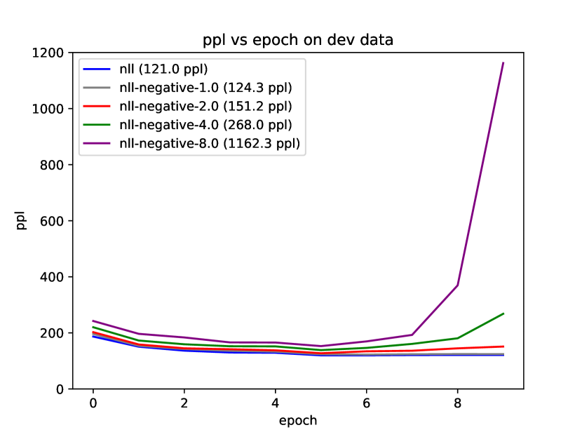
(b) Dev perplexity (positive data).

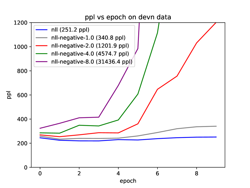
(c) Dev perplexity (negative data).

Figure 1: Perplexity on train, dev, and negative dev data for various training methods (small LSTM).

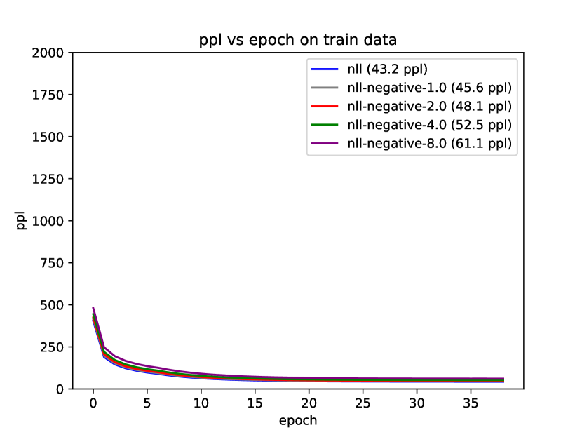
(d) Train perplexity.

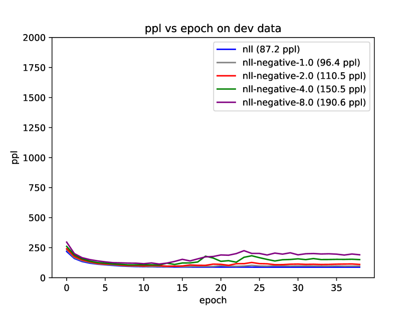
(e) Dev perplexity (positive data).

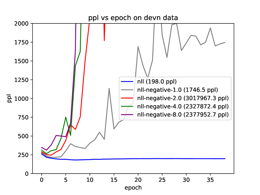
(f) Dev perplexity (negative data).

Figure 2: Perplexity on train, dev, and negative dev data for various training methods (med LSTM).

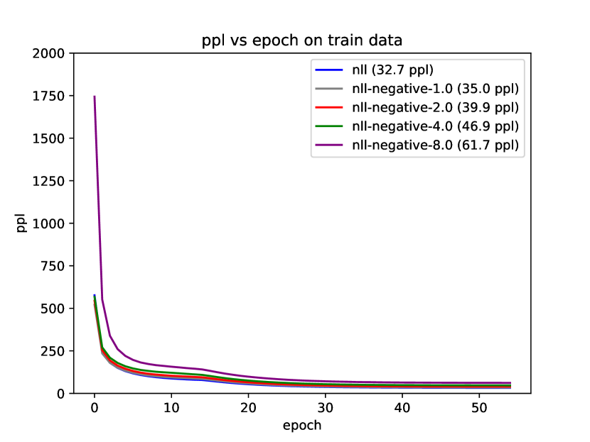
(a) Train perplexity.

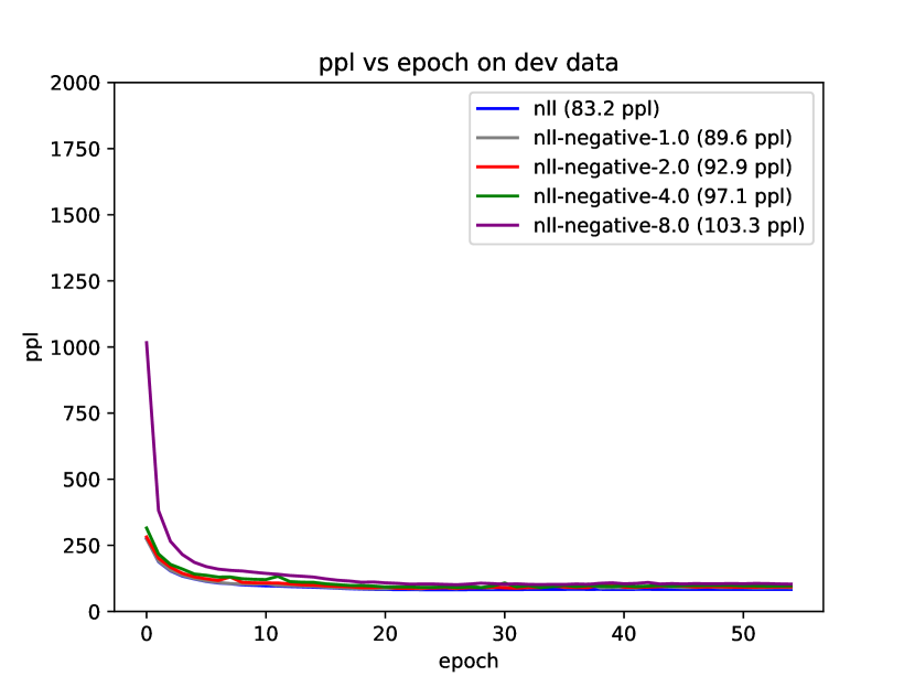
(b) Dev perplexity (positive data).

(c) Dev perplexity (negative data).

Figure 3: Perplexity on train, dev, and negative dev data for various training methods (large LSTM).

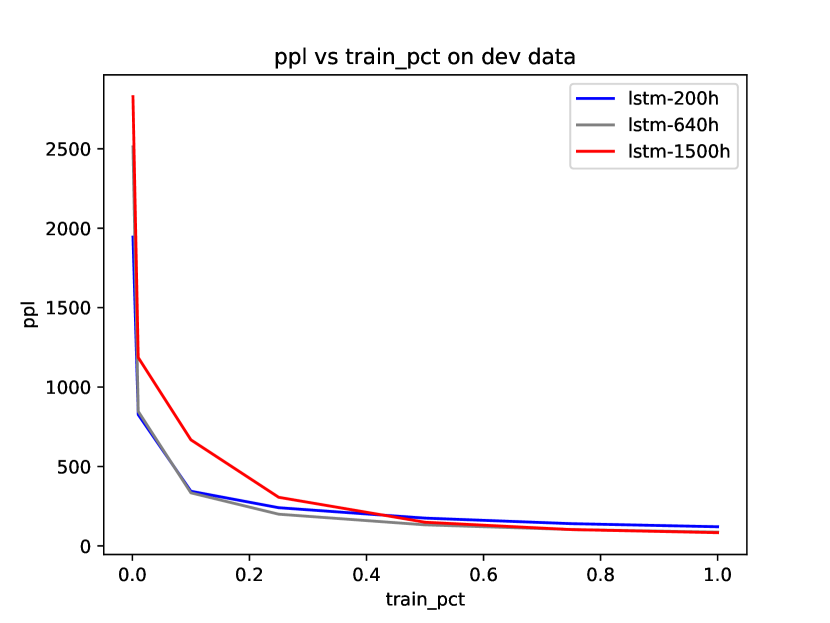
(a) Positive perplexity.

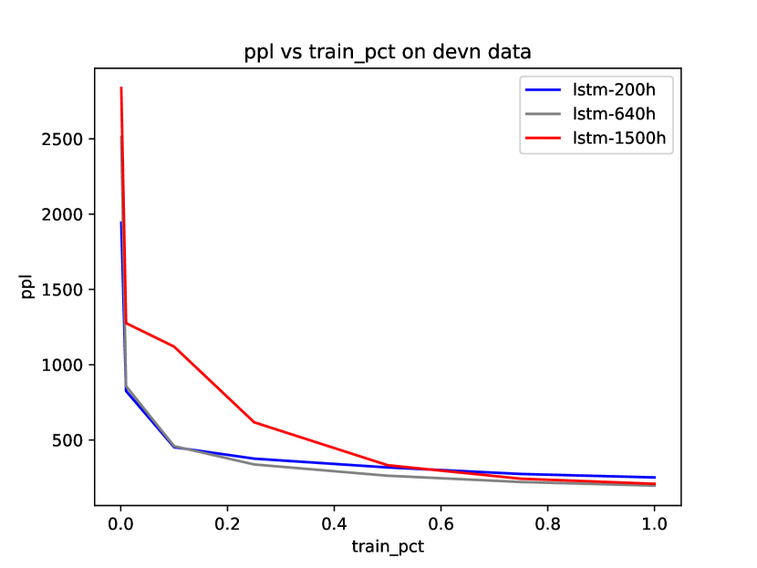
(b) Negative perplexity.

(c) Positive vs negative perplexity.

Figure 4: (a) & (b): the positive and negative effects of more training data. Portion of training data increases along x-axes, and y-axes is perplexity. (c): positive vs negative ppl for various models.

Here we study the extent to which a model learns undesirable tri-gram signals with negative data. We evaluate how well various language models perform on both positive and negative data. A language model should not only faithfully model the positive data, but it should also fail to model the negative data. That is, the best language models should ascribe higher probability (lower perplexity) to positive data and ascribe lower probability (higher perplexity) to negative data. We train each LSTM model (small, medium, and large) while varying $\alpha\in\{0,1,2,4,8\}$ for each of the three LSTMs ($\alpha=0$ is the traditional LSTM model in which we train with negative log-likelihood on the positive data). We plot the results in three figures, corresponding to small (Figure 3), medium (Figure 3), and large (Figure 3) LSTMs. Each figure contains three plots, demonstrating the models’ perplexity results, after each epoch, on the positive training data, the positive dev data, and the negative dev data. We also report the final perplexity that each model achieves in the plot legends.

First, focusing on the “nll” baselines, which are LSTMs trained only on the positive data with negative log likelihood, we see that for all three models the perplexity on the positive development data improves over time, as expected. However, the negative perplexity also improves: additional training epochs allow the three models to (undesirably) learn the negative tri-gram data. Fortunately, this behavior does not last forever, and the models begin to recover slightly (after about 15 epochs for the large LSTM). Looking across the plots for the three LSTM sizes, as the number of parameters increases (to 200, 650 and 1500 hidden units), we see that positive perplexity decreases, as expected. However, the increase in capacity also allows the model to fit the negative data better, providing evidence for an increased reliance on n-gram signals. Finally, in Figures 4(a)&4(b), as we vary the amount of positive training data, we observe a decrease in both positive and negative perplexity.

Our results indicate for models trained only on positive data, that increasing the amount of computation, the amount of model capacity, and the amount of positive training data, increases the model’s ability to fit both the positive and negative data. Of course, one explanation might be that n-grams are highly correlated with real English text, and there is a case to be made for this. However, examining sample sentences (some shown in the appendix in Figures 9&10), indicates that these sentences are different enough from natural language to quell major concerns. More importantly, if n-grams and English text were too tightly correlated, then it should be difficult to unmodel the n-grams without unmodeling the positive English text. So what happens when we employ negative data at train time?

Revisiting Figures 3, LABEL:, 3, LABEL: and 3, we see for all three LSTMs increasing the weight on the negative term of the loss function causes the models to aggressively unmodel the negative data. While the perplexity also increases on the positive data, it does not increase nearly as dramatically as on the negative data, except for the small LSTM when using a large weight on the negative term. Hence we can successfully remove the n-gram signal without damaging the overall language model.

We also plot the positive (x-axis) and negative (y-axis) perplexities in a scatter plot for each of the above models, as well as four transformer models (GPT2) of different sizes[33]. The intent is to see, for each model family, how changes in positive perplexity correspond to changes in negative perplexity. What we observe (Figure 4(c)) is that for each model family, when trained only on positive data, that as the positive perplexity decreases, so does the negative perplexity. While the transformers have a slightly higher perplexity on negative data than the LSTMs — perhaps not surprising given the known recency bias of LSTMs [34] — they also exhibit this trend. However note that when we train the LSTMs with the negative data, they have far worse perplexity on the negative data than even the transformers, while their perplexities on the positive data is only slightly decreased.

4.3 Results: attenuating n-grams improves syntax in language models

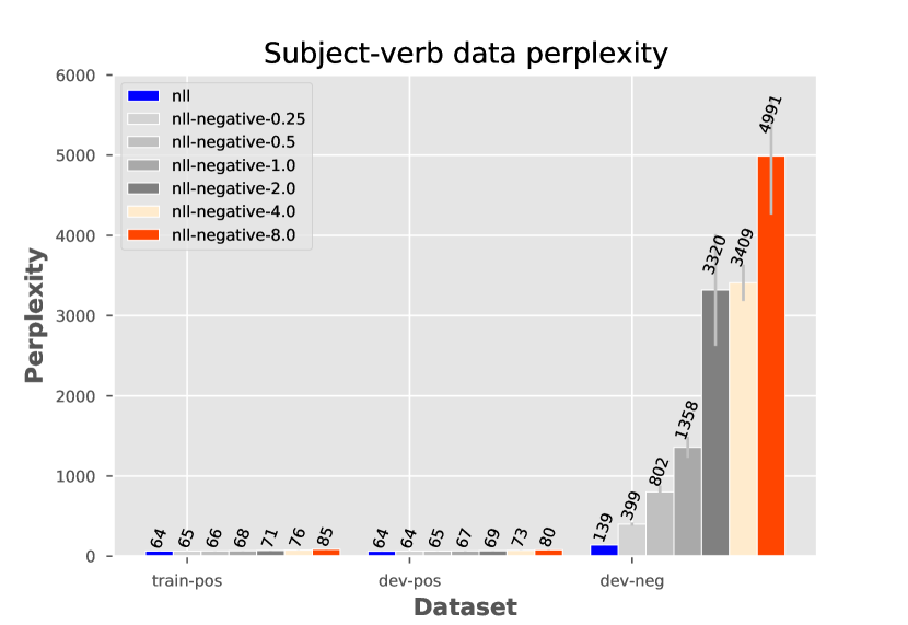
(a) Perplexity (LSTM large/1500h).

(b) Perplexity (GPT2).

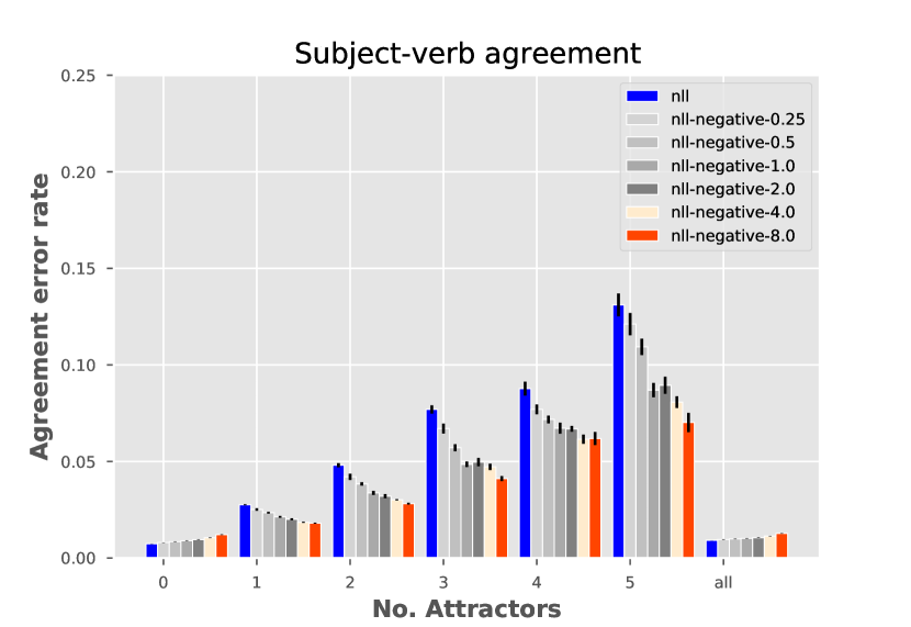
(c) Agreement error (LSTM large/1500h).

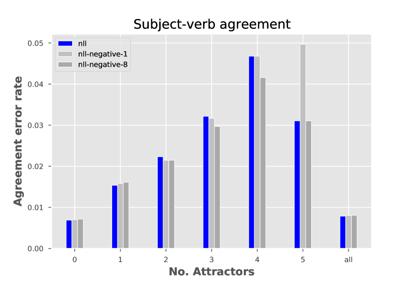
(d) Agreement error (GPT2).

Figure 5: Subject-verb agreement task with language models. Negative data are tri-gram generated.

In the introduction, we gave an example of a sentence where n-gram statistics might prove misleading, because the verb that makes the sentence ungrammatical is more common and co-occurs more frequently with the other words in the dataset. It is unlikely that LSTMs have an inductive bias to overcome such signals, and indeed we saw in the previous experiment that they learn n-gram statistics. We also saw that we can successfully attenuate these statistics with negative data, but does this cause the model to favor more desirable syntactic signals? We now turn to a subject-verb agreement task [23] to find evidence for the hypothesis that removing n-grams allows the model to handle longer-distance syntactic dependencies.

The subject verb agreement task is to determine if the subject of a sentence agrees with the verb. For example, in “the keys are on the table,” the subject “keys” must agree with the verb “are” in number, hence, “the keys is on the table” is incorrect [23]. In general there might be an intervening phrase between “keys” and “are” making the problem challenging as in “The keys to the cabinet are on the table.” Here, the singular noun cabinet, which has an opposite number to “keys”, is an attractor which could confuse the model. There might be arbitrarily many of these intervening attractors and the subject and verb may in general be arbitrarily far apart. The results are thus organized by the number of attractors between the subject and the verb. The more attractors, the more difficult the task. The language model has correctly predicted agreement if it assigns higher probability to the (grammatical) sentence with the correct verb than the (ungrammatical) sentence with the incorrect verb.

Table 1: Error-rate comparison on subject-verb agreement data.

method	attr=0	1	2	3	4	5
LSTM/nll (1500h)	0.7	2.8	4.7	7.3	8.9	12.9
LSTM/nll-neg-8 (1500h)	1.2	1.8	2.8	4.1	6.2	7.0
$\Delta$	0.5	-1.0	-1.9	-3.2	-2.7	-5.9
GPT2 (110M, zero-shot)	7.7	14.8	21.1	24.9	21.5	24.2
GPT2+nll	0.7	1.5	2.2	3.2	4.7	3.1
GPT2+nll-neg-8	0.7	1.6	2.1	3.0	4.2	3.1
$\Delta$ (nll, nll-neg-8)	0.0	0.1	-0.1	-0.2	-0.5	0.0

We employ the same splitting strategy as prior work (ibid), and train the small and large LSTMs for 10 and 20 epochs respectively. We also fine-tune and evaluate a pretrained GPT2 model on the same splits (see Appendix D.1 for fine-tuning details).

Table 1 shows that, in general, training or fine-tuning by attenuating n-gram statistics improves language models’ ability to associate verbs with their correct subject. As we increase the weight on the negative data objective, model perplexity on the negative development data increases (Figures 5(a) & 5(b)) and for the LSTM, the subject-verb agreement error decreases (Figure 5(c)), though this trend is mixed for GPT-2 (Figure 5(d)). For the LSTM, this performance gap increases as the number of attractors increases while for GPT-2 the performance gap is roughly constant with most benefit at four attractors. It is also interesting to note that when there are no attractors, the negative data actually hurts LSTM performance on the task. The reason is that without any attractors, the subject and verb are close and the tri-grams serve as a good proxy for syntax, despite the flaws we highlighted.

5 Conclusion

We proposed a method for detecting and attenuating undesirable signals in language models. When applied to detecting n-grams, we found that existing models rely on them possibly at the expense of more syntactic signals. When applied to attenuating n-grams at train-time, our method added an inductive bias that succesfully pushed the more powerful language models (LSTMs, GPT2) away from the less powerful models (tri-grams) and towards hypothesis classes that performed better at syntactic tasks. Perplexity was barely affected. The method is a general way, like data augmentation, of imbuing the model with inductive bias. Indeed, while we focused on n-grams in this work, the method is much more general and we can apply it as a tool to detect and attenuate other undesirable signals in the data, like gender bias. In future work, we also want to explore ways of incorporating the idea into masked language models, and explore alternatives to negative data like contrastive learning, that more directly incorporate the negative model into the loss function.

Appendix A Additional experiments and details for the subject-verb data

Figure 6: A block diagram of the anti-modeling training procedure. A negative generative model $\mathcal{M}^{\prime}$ is automatically fit to the positive data $\mathcal{D}$ and then used to generate negative data $\mathcal{D}^{\prime}$. Both positive and negative data can then be used in the appropriate way to train the final model $\mathcal{M}$. Red boxes indicate negative models and data, green boxes indicate positive model and data.

A.1 Subject-verb data

Here we provide more details of the subject-verb data. We employ the same split of the data as prior work as best we can, based on their code, using the same random splitting strategy with the same random seed and the same proportions of train, test and dev [23]. We then organized the data into the number of intervening attractors, achieving data statistics very close, but not exactly identical to another piece of prior work [19]. We report our data statistics for the testing set in Table 2, which we can compare with Table 1 in prior work to see the similarity in our data statistics (ibid). We report the % of instances that each set represents as a percentage of the set of data with opposite number attractors and as a percentage of the full test set (which is larger because it includes cases in which there are attractors of the same number or cases with more than 5 attractors).

Table 2: Subject-verb agreement data statistics.

# Attractors	# Instances	% Instances ($n=1\ldots 5$)	% Instances (full test)
$n=0$	1,146,256	94.65%	80.75%
$n=1$	51,714	4.34%	3.71%
$n=2$	9,151	0.78%	0.66%
$n=3$	1,942	0.17%	0.14%
$n=4$	546	0.05%	0.04%
$n=5$	161	<0.01%	<0.01%
$n\in\{0\ldots 5\}$	1,211,033	100%	85%
all	1,419,491		100%

A.2 Subject-verb agreement comparison with related work

We note that our goal is not to achieve state of the art on the subject-verb agreement task, but rather our goal is to use this task to help provide evidence for our hypothesis: attenuating n-gram signals improves syntactic ability. Nevertheless, it might be useful to compare how our language models perform with other results reported in the literature on this task, which we do in Table 3.

We caution that due to various factors, and different practices employed throughout the literature, that these results are not directly comparable. We attempt a comprehensive set of differences here:

• We compute the probability of the full sentences (grammatical and ungrammatical) when making subject-verb agreement judgements [27, 13], but other work only computes the probability of the tokens up to the verb [23, 19].

• BERT and BART models are trained on Wikipedia and hence are exposed to the sentences in the test set of the subject-verb agreement (which are all from Wikipedia also).

• BERT and BART models employ a different tokenization scheme that can split words into multiple pieces. Sentences for which the target verb is split into multiple pieces are filtered out of the BERT evaluation data. If it happens to be the case that these words are relatively rarer, then it might mean that this subset of the data is slightly easier.

• BERT and BART models are evaluated on a subset of the evaluation data. Sentences in which the main verb are is/are are pruned because in copula constructions, the objects after the verb can provide syntactic cues for this task (e.g., the object “friends” has the same number as “girls” in the sentence “the girls are friends.”); however, note that the example sentence we employ in the introduction is also copular and this is a case in which the object following the verb functions as a distractor in the sense that the number of the object disagrees with the subject. Thus, it is unclear how this pruning might affect the results.

If we compare the first two rows of Table 3, we see that the negative data training method allows a model with just 200 hidden units (8M parameters) to close the gap with the 1500 hidden-unit LSTM (69M parameters) in some categories; though, performance is still worse. If we look at the negative data training method on the 1500 hidden-unit LSTM, we see that it greatly improves over the same LSTM trained with positive data only (with the exception of the 0 attractor case, which we discussed earlier in the experiments section).

When we compare with other results reported in the literature, such as recursive neural network grammars (RRNG-$\star$), that also add an inductive bias to language, we see that our method has a substantially lower error rate. However, our method employs the entire sentence to judge grammaticallity and their method only employs up to the verb. Moreover, it is unclear how many hidden units their model employs and it is likely that much of our performance increase is simply because our 1500 hidden unit LSTM is larger.

Now interestingly, our 84M parameter LSTM trained with negative data (third row) performs much better than BART, a transformer-based denoising auto-encoder, that has 400M parameters; and performs comparably to BERT (300M parameters). This is remarkable especially since the training data of BART and BERT include all the testing sentences in this task, and these massive models dwarf our relatively modest LSTM.

A.3 Other negative n-gram distributions: bi-grams and 4-grams

For our experiments in the main paper we chose word tri-grams as our negative distribution as we suspected them to be a sweet spot for our dataset: they are powerful enough to generate reasonable language-like sentences, but not powerful enough to overfit the positive training data (and thus generate negative data that is too similar). Our results for the 2-grams and 4-gram negative models still demonstrate some benefits, but they are not as pronounced or uniform as for the tri-gram models.

We present results for the small 200 hidden unit LSTM in Figure 7. We present results for the large 1500 hidden unit LSTM in Figure 8. The results confirm our suspicions that a 4-gram is too strong of an anti-model for the relatively small train-set of the subject-verb dataset (most of the data is relegated to the test-set in order to allow more accurate analysis). One indication of this is that for the 1-attractor, the models that employs the 4-grams for negative data performs worse than the model that only employs positive data, which was not the case for tri-grams. For the larger LSTM, we also see that 4-grams are problematic for some larger attractor conditions too. We suspect that 4-grams are overfitting the training set and that the sentences they generate are too similar to the positive sentences after which they are modeled. So using a negative model that is too powerful is not ideal.

On the other hand, using a model that is too weak, like bi-grams, is not effective as using a more powerful negative model, like tri-grams (this is likely to be particular to the subject-verb training set, and others like it that are relatively small, so one should not generalize too far here). For the smaller LSTM, there is only an improvement for smaller values of $\alpha$ and the improvement is not nearly as pronounced as in the tri-gram version. For the larger LSTM, there are improvements across all values of $\alpha$, but the improvement again is not as large as in the tri-gram version.

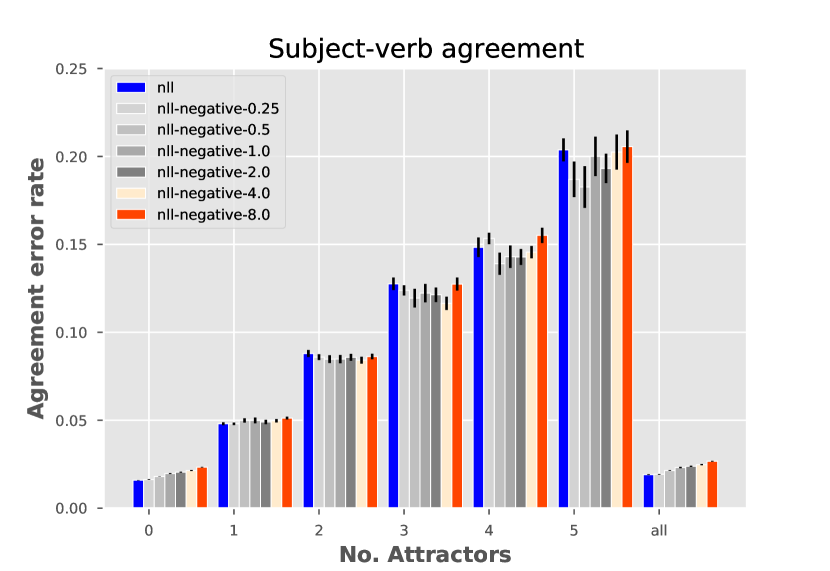
(a) Agreement error (negative: bi-grams).

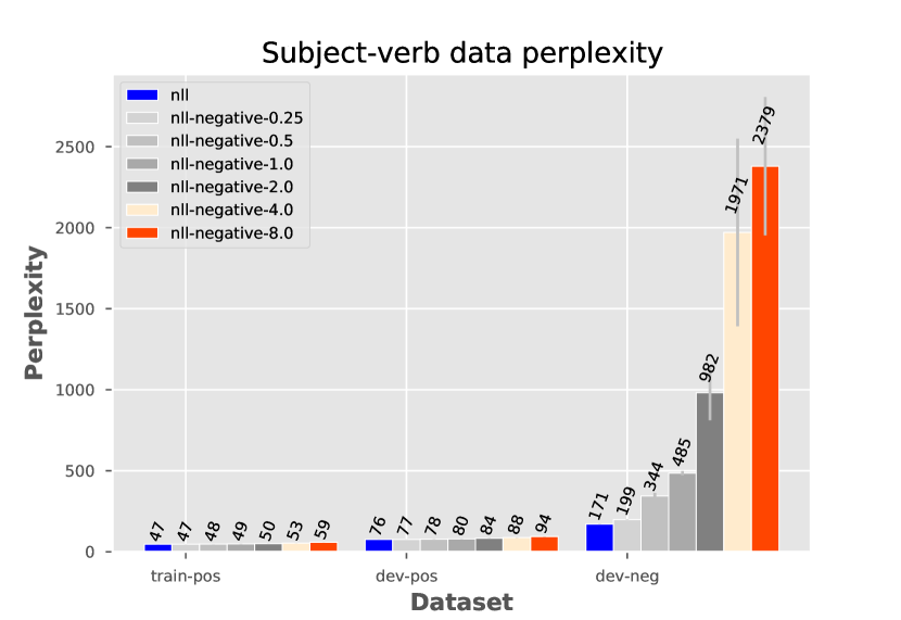
(b) Agreement data ppl (negative: bi-grams)

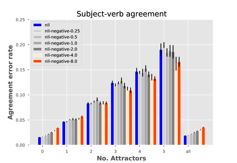
(c) Agreement error (negative: 4-grams).

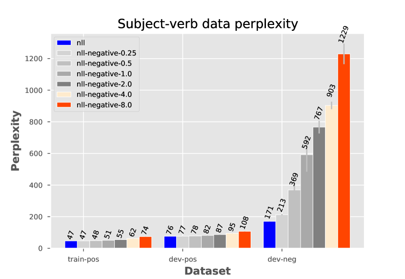
(d) Agreement data ppl (negative: 4-grams).

Figure 7: Subject-verb agreement data with the 200 hidden unit LSTM.

(a) Agreement error (negative: bi-grams).

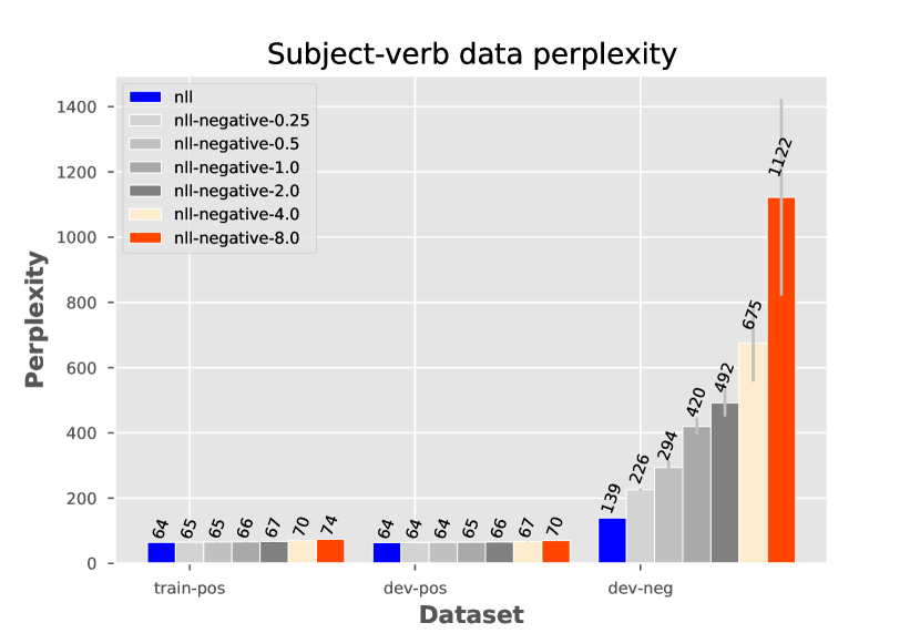
(b) Agreement data ppl (negative: bi-grams)

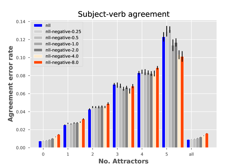
(c) Agreement error (negative: 4-grams).

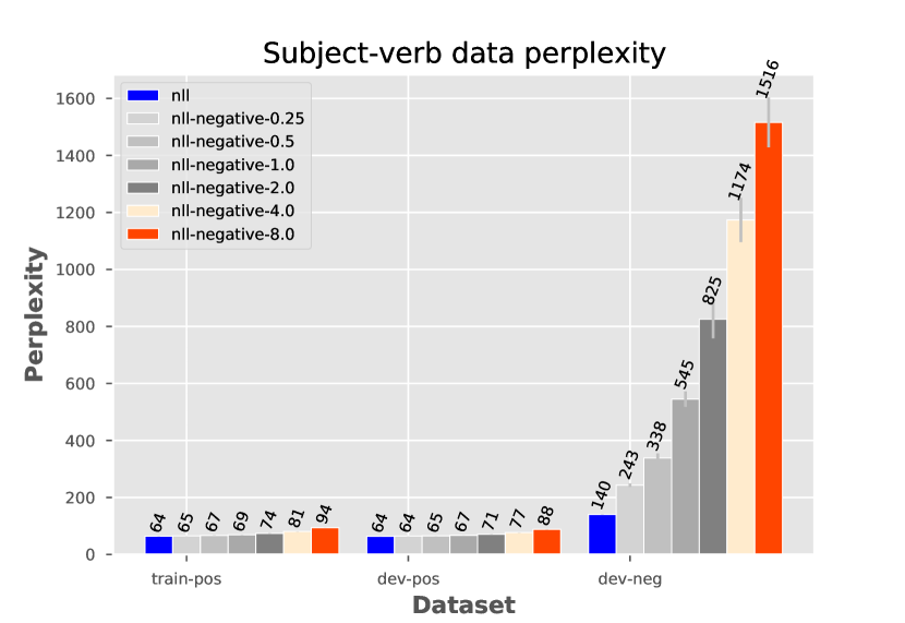
(d) Agreement data ppl (negative: 4-grams).

Figure 8: Subject-verb agreement data with the 1500 hidden unit LSTM.

method	attr=0	1	2	3	4	5
nll (1500h)	0.7	2.8	4.7	7.3	8.9	12.9
nll-neg-8.0 (200h)	2.8	4.2	6.5	8.9	10.2	11.7
nll-neg-8.0 (1500h)	1.2	1.8	2.8	4.1	6.2	7.0
RNNG-TD [19]			5.5	7.8	8.9
RNNG-LC [19]			5.4	8.2	9.9
RNNG-BU [19]			5.7	8.5	9.7
LSTM 50h [23, 19]	2.4	8.0	15.7	26.1	34.6
LSTM 150h [19]	1.5	4.5	9.0	14.3	17.6
LSTM 250h [19]	1.4	3.3	5.9	9.7	13.9
LSTM 350h [19]	1.3	3.0	5.7	9.7	13.8
1B Word LSTM [17, 19]	2.8	8.0	14.0	21.8	20.0
BERT (340M params)* [13, 8]		3	3	4	3
BART (400M params)*[16, 22]		3.8	4.1	6.0	6.7
GPT (110M params) [32, 40]		18	24	31	30

Table 3: Error-rate comparison to other language models on the subject-verb agreement data. Note these results are not directly comparable for reasons stated in the text: in short, BERT and BART are trained on data that includes the test sentences and are also evaluated on a subset of the official test-set. The other LSTMs and RGNN models only model sentences up to the main verb. *trainining set includes test data.

Appendix B Results on targeted syntactic evaluation

We also evaluate our models on an additional syntactic tasks with artificial data from prior work that is automatically generated from hand-crafted grammars [27]. Since the models we study in this work are trained on the subject-verb agreement task [23], which is an order of magnitude smaller than the training data of prior work (ibid), it turns out that more than two-thirds of the data has an example with an out-of-vocabulary (OOV) word, and that in 24% of the cases, this out of vocabulary word happened to be the word (the target word) that distinguishes the grammatical version of the sentence from the ungrammatical version. We present three sets of results, one on the entire dataset (Table 6), one on a subset comprising examples for which the target is not OOV (Table 4) and one on a subset comprising examples for which no word is OOV (Table 5) . This latter is done because most words in these sentences are determiners and other fillers and thus the OOVs might be the cues relevant to perform the task. Highlighted rows indicate those for which the negative data seemed to improve the baseline of negative log likelihood (nll) on the positive data only.

Table 4: LSTM 200h results on Marvin & Linzen subset without oov targets.

	nll	nll-neg-1.0	nll-neg-2.0	nll-neg-4.0	nll-neg-8.0
Subject-verb agreement
Simple	$1.00$ $\pm 0.00$	$1.00$ $\pm 0.00$	$1.00$ $\pm 0.00$	$0.92$ $\pm 0.03$	$0.84$ $\pm 0.06$
In a sentential complement	$0.86$ $\pm 0.01$	$0.85$ $\pm 0.02$	$0.86$ $\pm 0.02$	$0.77$ $\pm 0.03$	$0.73$ $\pm 0.03$
Short VP coordination	$0.95$ $\pm 0.02$	$0.99$ $\pm 0.00$	$0.95$ $\pm 0.01$	$0.77$ $\pm 0.05$	$0.74$ $\pm 0.06$
Long VP coordination	$0.62$ $\pm 0.01$	$0.66$ $\pm 0.04$	$0.59$ $\pm 0.01$	$0.59$ $\pm 0.03$	$0.56$ $\pm 0.02$
Across a prepositional phrase	$0.96$ $\pm 0.00$	$0.96$ $\pm 0.00$	$0.92$ $\pm 0.03$	$0.78$ $\pm 0.07$	$0.74$ $\pm 0.07$
Across a subject relative clause	$0.95$ $\pm 0.02$	$0.98$ $\pm 0.01$	$0.95$ $\pm 0.02$	$0.83$ $\pm 0.04$	$0.77$ $\pm 0.07$
Across an object relative clause	$0.76$ $\pm 0.02$	$0.79$ $\pm 0.02$	$0.80$ $\pm 0.02$	$0.65$ $\pm 0.04$	$0.63$ $\pm 0.05$
Across an objective relative (no that)	$0.70$ $\pm 0.02$	$0.72$ $\pm 0.02$	$0.74$ $\pm 0.03$	$0.62$ $\pm 0.04$	$0.58$ $\pm 0.03$
In an object relative clause	$0.64$ $\pm 0.02$	$0.64$ $\pm 0.01$	$0.64$ $\pm 0.01$	$0.62$ $\pm 0.01$	$0.59$ $\pm 0.01$
In an object relative (no that)	$0.63$ $\pm 0.02$	$0.60$ $\pm 0.01$	$0.64$ $\pm 0.01$	$0.60$ $\pm 0.01$	$0.56$ $\pm 0.02$
Reflexive anaphora
Simple (RA)	$0.84$ $\pm 0.03$	$0.79$ $\pm 0.04$	$0.79$ $\pm 0.04$	$0.65$ $\pm 0.05$	$0.66$ $\pm 0.04$
In a sentential complement	$0.86$ $\pm 0.01$	$0.85$ $\pm 0.02$	$0.86$ $\pm 0.02$	$0.77$ $\pm 0.03$	$0.73$ $\pm 0.03$
Across a relative clause (RA)	$0.75$ $\pm 0.01$	$0.71$ $\pm 0.03$	$0.67$ $\pm 0.03$	$0.67$ $\pm 0.04$	$0.66$ $\pm 0.02$
Negative polarity items
Simple (NPI)	$0.53$ $\pm 0.01$	$0.55$ $\pm 0.02$	$0.53$ $\pm 0.02$	$0.54$ $\pm 0.01$	$0.49$ $\pm 0.02$
Across a relative clause (NPI)	$0.56$ $\pm 0.01$	$0.57$ $\pm 0.01$	$0.57$ $\pm 0.01$	$0.54$ $\pm 0.01$	$0.54$ $\pm 0.02$
All	$0.72$ $\pm 0.01$	$0.73$ $\pm 0.01$	$0.73$ $\pm 0.01$	$0.65$ $\pm 0.02$	$0.62$ $\pm 0.03$

Table 5: LSTM 200h results on Marvin & Linzen subset without OOV words.

	nll	nll-neg-1.0	nll-neg-2.0	nll-neg-4.0	nll-neg-8.0
Subject-verb agreement
Simple	$1.00$ $\pm 0.00$	$1.00$ $\pm 0.00$	$1.00$ $\pm 0.00$	$0.76$ $\pm 0.00$	$0.81$ $\pm 0.00$
In a sentential complement	$0.89$ $\pm 0.03$	$0.81$ $\pm 0.02$	$0.89$ $\pm 0.05$	$0.71$ $\pm 0.00$	$0.69$ $\pm 0.00$
Short VP coordination	$0.99$ $\pm 0.01$	$0.94$ $\pm 0.02$	$0.99$ $\pm 0.01$	$0.57$ $\pm 0.11$	$0.69$ $\pm 0.00$
Long VP coordination	$0.65$ $\pm 0.02$	$0.59$ $\pm 0.02$	$0.60$ $\pm 0.00$	$0.51$ $\pm 0.03$	$0.51$ $\pm 0.00$
Across a prepositional phrase	$0.96$ $\pm 0.01$	$0.97$ $\pm 0.00$	$0.97$ $\pm 0.01$	$0.58$ $\pm 0.03$	$0.61$ $\pm 0.00$
Across a subject relative clause	$0.95$ $\pm 0.01$	$0.98$ $\pm 0.01$	$0.98$ $\pm 0.01$	$0.62$ $\pm 0.05$	$0.68$ $\pm 0.00$
Across an object relative clause	$0.72$ $\pm 0.03$	$0.71$ $\pm 0.03$	$0.79$ $\pm 0.06$	$0.52$ $\pm 0.01$	$0.57$ $\pm 0.00$
Across an objective relative (no that)	$0.67$ $\pm 0.02$	$0.73$ $\pm 0.02$	$0.74$ $\pm 0.01$	$0.46$ $\pm 0.02$	$0.54$ $\pm 0.00$
In an object relative clause	$0.64$ $\pm 0.01$	$0.63$ $\pm 0.02$	$0.64$ $\pm 0.01$	$0.59$ $\pm 0.01$	$0.59$ $\pm 0.00$
In an object relative (no that)	$0.65$ $\pm 0.01$	$0.61$ $\pm 0.02$	$0.60$ $\pm 0.04$	$0.57$ $\pm 0.02$	$0.63$ $\pm 0.00$
Reflexive anaphora
Simple (RA)	$0.84$ $\pm 0.03$	$0.74$ $\pm 0.05$	$0.87$ $\pm 0.04$	$0.69$ $\pm 0.10$	$0.57$ $\pm 0.00$
In a sentential complement	$0.89$ $\pm 0.03$	$0.81$ $\pm 0.02$	$0.89$ $\pm 0.05$	$0.71$ $\pm 0.00$	$0.69$ $\pm 0.00$
Across a relative clause (RA)	$0.72$ $\pm 0.02$	$0.72$ $\pm 0.04$	$0.77$ $\pm 0.01$	$0.70$ $\pm 0.00$	$0.71$ $\pm 0.00$
Negative polarity items
Simple (NPI)	$0.54$ $\pm 0.01$	$0.54$ $\pm 0.02$	$0.61$ $\pm 0.04$	$0.55$ $\pm 0.09$	$0.51$ $\pm 0.00$
Across a relative clause (NPI)	$0.56$ $\pm 0.01$	$0.59$ $\pm 0.01$	$0.60$ $\pm 0.01$	$0.57$ $\pm 0.02$	$0.55$ $\pm 0.00$
All	$0.72$ $\pm 0.01$	$0.72$ $\pm 0.00$	$0.74$ $\pm 0.00$	$0.56$ $\pm 0.01$	$0.60$ $\pm 0.00$

Table 6: LSTM 200h results on all Marvin & Linzen data [27].

	nll	nll-neg-1.0	nll-neg-2.0	nll-neg-4.0	nll-neg-8.0
Subject-verb agreement
Simple	$0.74$ $\pm 0.01$	$0.73$ $\pm 0.01$	$0.75$ $\pm 0.01$	$0.73$ $\pm 0.01$	$0.73$ $\pm 0.01$
In a sentential complement	$0.75$ $\pm 0.02$	$0.71$ $\pm 0.02$	$0.73$ $\pm 0.02$	$0.72$ $\pm 0.01$	$0.69$ $\pm 0.02$
Short VP coordination	$0.72$ $\pm 0.01$	$0.71$ $\pm 0.01$	$0.72$ $\pm 0.01$	$0.74$ $\pm 0.01$	$0.73$ $\pm 0.01$
Long VP coordination	$0.63$ $\pm 0.02$	$0.61$ $\pm 0.01$	$0.62$ $\pm 0.02$	$0.60$ $\pm 0.01$	$0.58$ $\pm 0.01$
Across a prepositional phrase	$0.76$ $\pm 0.00$	$0.77$ $\pm 0.00$	$0.78$ $\pm 0.00$	$0.78$ $\pm 0.00$	$0.78$ $\pm 0.00$
Across a subject relative clause	$0.69$ $\pm 0.01$	$0.72$ $\pm 0.01$	$0.73$ $\pm 0.00$	$0.73$ $\pm 0.00$	$0.72$ $\pm 0.00$
Across an object relative clause	$0.65$ $\pm 0.02$	$0.71$ $\pm 0.02$	$0.69$ $\pm 0.02$	$0.72$ $\pm 0.02$	$0.76$ $\pm 0.01$
Across an objective relative (no that)	$0.63$ $\pm 0.02$	$0.71$ $\pm 0.01$	$0.71$ $\pm 0.02$	$0.72$ $\pm 0.01$	$0.74$ $\pm 0.02$
In an object relative clause	$0.60$ $\pm 0.01$	$0.60$ $\pm 0.01$	$0.59$ $\pm 0.00$	$0.57$ $\pm 0.01$	$0.55$ $\pm 0.01$
In an object relative (no that)	$0.60$ $\pm 0.01$	$0.60$ $\pm 0.01$	$0.60$ $\pm 0.01$	$0.58$ $\pm 0.01$	$0.57$ $\pm 0.01$
Reflexive anaphora
Simple (RA)	$0.79$ $\pm 0.02$	$0.70$ $\pm 0.03$	$0.72$ $\pm 0.03$	$0.67$ $\pm 0.03$	$0.63$ $\pm 0.03$
In a sentential complement	$0.75$ $\pm 0.02$	$0.71$ $\pm 0.02$	$0.73$ $\pm 0.02$	$0.72$ $\pm 0.01$	$0.69$ $\pm 0.02$
Across a relative clause (RA)	$0.69$ $\pm 0.02$	$0.67$ $\pm 0.01$	$0.65$ $\pm 0.01$	$0.67$ $\pm 0.01$	$0.69$ $\pm 0.03$
Negative polarity items
Simple (NPI)	$0.57$ $\pm 0.01$	$0.57$ $\pm 0.01$	$0.56$ $\pm 0.01$	$0.58$ $\pm 0.01$	$0.55$ $\pm 0.01$
Across a relative clause (NPI)	$0.58$ $\pm 0.00$	$0.58$ $\pm 0.01$	$0.58$ $\pm 0.00$	$0.57$ $\pm 0.01$	$0.57$ $\pm 0.01$
All	$0.65$ $\pm 0.01$	$0.67$ $\pm 0.00$	$0.67$ $\pm 0.00$	$0.67$ $\pm 0.00$	$0.67$ $\pm 0.01$

Appendix C Negative data examples

Here we provide some examples of the type of negative word-based tri-gram data we employ for training and evaluation. In Figure 9 we show a few random negative sentences from a model trained on the PTB dev set. In Figure 10, we show a few random negative sentences from a mdoel trained on the subject-verb agreement dev set. Some sentences resemble language, while others are complete gibberish. The training sentences tend to be more language like since those models are always pre-conditioned on appropriate context. The dev-data is generated in a single-go without re-conditioning.

for instance for a piece on local tv stations and sells some of its $ N the dow jones transportation average second in size only to the customer .

he visits the same time .

today of all the witnesses both congressmen and industry said .

the ads touted fidelity ’s automated <unk> beneath the huge drop in stock prices firmed up again as traders sold big baskets of stock .

moody ’s investors service inc. downgraded its ratings on the chicago market makers to get advertisers to use their clout to help insure the integrity of the home fans in this country .

Figure 9: Sampling of the tri-grams version of the official PTB dev set (with Mikolov’s pre-processing). The period indicates end of the line, N indicates a number and <unk> is a symbol that replaces the rare words in the original corpus, but that the tri-gram model still learns to generate.

NNP is the NN VBZ the post ’s other major began “ VBG their way to prove that they face off against a sourced recreation with appropriate links to the NNS of flies or NNS on the west are available .

when a spell NN , brain waves and body movements while they may contain useful info , 5 , and as strong as physical force .

the arms show 17 gold NNS on the wars of that name is just east of the increased potential energy . and if NNS , and when at the temple .

the saxon NNP river then flows from NNP .

the highest point in the plane p NN to the north and south branch , ford branch , both of these two lines .

on the western edge of NNP .

collaboration generally is a combination of natural circulation include NNS and of the VBG fan input or adjacent to the west represent NNP NNS , NNS and NNP ) uses two proprietary standards instead of four tunnels that have common elements from all major NNS ; examples include red NNP , NNP NNP , st .

only a few sandy beaches , the NN and a bit too much

Figure 10: Tri-gram version of Linzen&Goldberg subject-verb agreement data set. The tri-gram is trained on the development portion of the data. Rare words are replaced with their part of speech: NN is a singular noun, NNS a plural noun, NNP a singular proper noun, VBZ a present singular verb, VBG a gerund, etc.

Appendix D Fine-tuning by attenuating n-gram statistics

In the experiments above, we demonstrated that language model training by attenuating tri-gram statistics improves models’ ability to both rule out "negative" sentences (Section 4.2) and navigate long-distance syntactic dependencies (Section 4.3) across a variety of architectures, including GPT2.

In this section, we explore fine-tuning GPT2 using our method in greater detail. Overall, our results indicate that tri-gram attenuation a) increases negative-data perplexity without harming positive-data perplexity (Section D.2) and b) improves GPT2’s performance across most of the long-distance constructions in an additional syntactic evaluation task (Section D.3). This serves as preliminary evidence that n-gram attenuation during fine-tuning is an effective way to improve GPT2’s interpretation of long-distance dependencies without sacrificing language model quality and without using additional data beyond the fine-tuning set itself. We leave assessment of other Transformer architectures, as well as a detailed examination of the interaction between n-gram order and model quality, for future work.

D.1 Model & fine-tuning details

We fine-tune the base GPT2 model (110M parameters) via the HuggingFace library [39] . In all cases, we fine-tune for 10 epochs using the Adam optimizer [18] with decoupled weight decay regularization [25] as implemented in [39]. We use an initial learning rate of $5e-5$, $\epsilon=1e-8$, and clip gradients at $1$. We did not tune these hyperparameters, but rather used the default values given in HuggingFace.

For all datasets, we use the same train/dev/test splits as described above. For the Penn Treebank experiments in Section D.2, we use batches of size $16$ over text windows of length $20$ tokens. In all other experiments, we use batches of $32$ sentences. As in prior experiments, during training, we generate a "negative" version of each batch using an unsmoothed tri-gram language model trained beforehand using maximum likelihood estimation [24].

For each experiment, we report the results for a single fine-tuning/evaluation run. We leave robust estimation of invariance to random seed, settings of $\alpha$, and other hyperparameters for future work.

D.2 Results: detecting and attenuating n-grams

To inspect how tri-gram attenuation affects language model quality as fine-tuning progresses, we measure perplexity on the PTB train, dev, and "negative dev" sets (described in Section 4.1) after each training epoch. As was the case with the LSTMs, "positive" dev perplexity stays constant while the the negative-data objective causes "negative" dev perplexity to increase in the cases where $\alpha>0$ was used (Fig 11).

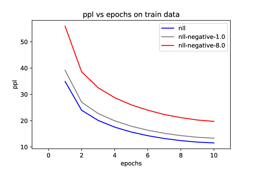
(a) Train perplexity.

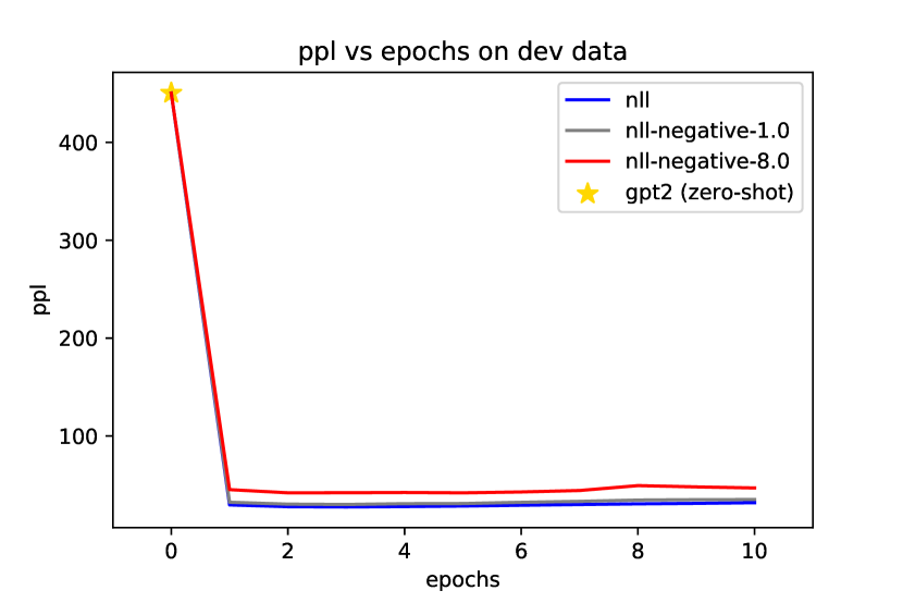
(b) Dev perplexity (positive data).

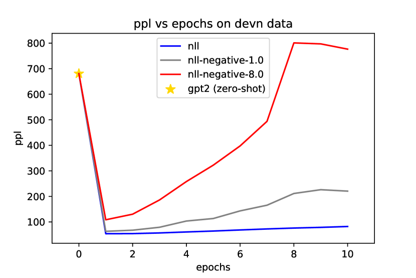
(c) Dev perplexity (negative data).

Figure 11: Perplexity on train, dev, and negative dev data (GPT-2).

D.3 Results on targeted syntactic evaluation

To evaluate whether fine-tuning with exorcism improves GPT2’s syntactic abilities, we fine-tune on the subject-verb agreement training set provided by [23] and, as in Section A.1, we evaluate on the syntactic constructions from [27].

Table 7 shows that fine-tuning with tri-gram attenuation improves the language model’s interpretation of many constructions. Most of the cases where our method hurt performance involve short-distance dependencies. For example, as noted in [27], dependencies within object relative clauses are local:

The farmer that the parents love swims.

*The farmer that the parents loves swims.

That is, "parents" and "love" must agree; the distractor is "farmer". Such cases show that exorcising away n-gram statistics can cause language models to misinterpret dependencies that are close together. Indeed, performance in both "within object RC" categories more-or-less decreased as exorcism strength ($\alpha$) increased. This suggests that n-gram attenuation during fine-tuning introduces a trade-off between optimizing the model to interpret long-distance dependencies at the expense of interpreting short-distance dependencies. We leave further investigation of this trade-off for future work.

Table 7: GPT2 results on Marvin & Linzen data [27]. Highlighted rows indicate those for which the mean of the "negative data" results mean(nll-neg-1, nll-neg-8) beat the maximum baseline score max(gpt2, nll).

	gpt2 (zero-shot)	nll	nll-neg-1	nll-neg-8
Subject-verb agreement
Simple	$0.89$ $\pm 0.00$	$\mathbf{0.99}$ $\pm 0.00$	$\mathbf{0.99}$ $\pm 0.00$	$0.94$ $\pm 0.00$
In a sentential complement	$0.84$ $\pm 0.00$	$0.92$ $\pm 0.00$	$\mathbf{0.93}$ $\pm 0.00$	$0.91$ $\pm 0.00$
Short VP coordination	$\mathbf{0.96}$ $\pm 0.00$	$\mathbf{0.96}$ $\pm 0.00$	$0.95$ $\pm 0.00$	$0.94$ $\pm 0.00$
Long VP coordination	$0.91$ $\pm 0.00$	$0.93$ $\pm 0.00$	$0.93$ $\pm 0.00$	$\mathbf{0.94}$ $\pm 0.00$
Across a prepositional phrase	$0.77$ $\pm 0.00$	$\mathbf{0.95}$ $\pm 0.00$	$\mathbf{0.95}$ $\pm 0.00$	$\mathbf{0.95}$ $\pm 0.00$
Across a subject relative clause	$0.72$ $\pm 0.00$	$0.93$ $\pm 0.00$	$0.92$ $\pm 0.00$	$\mathbf{0.94}$ $\pm 0.00$
Across an object relative clause	$0.84$ $\pm 0.00$	$0.92$ $\pm 0.00$	$0.93$ $\pm 0.00$	$\mathbf{0.94}$ $\pm 0.00$
Across an objective relative (no that)	$0.77$ $\pm 0.00$	$0.88$ $\pm 0.00$	$\mathbf{0.89}$ $\pm 0.00$	$\mathbf{0.89}$ $\pm 0.00$
In an object relative clause	$\mathbf{0.94}$ $\pm 0.00$	$0.79$ $\pm 0.00$	$0.75$ $\pm 0.00$	$0.77$ $\pm 0.00$
In an object relative (no that)	$\mathbf{0.89}$ $\pm 0.00$	$0.77$ $\pm 0.00$	$0.75$ $\pm 0.00$	$0.75$ $\pm 0.00$
Reflexive anaphora
Simple (RA)	$\mathbf{0.98}$ $\pm 0.00$	$0.92$ $\pm 0.00$	$0.94$ $\pm 0.00$	$0.94$ $\pm 0.00$
In a sentential complement (RA)	$\mathbf{0.88}$ $\pm 0.00$	$0.83$ $\pm 0.00$	$0.81$ $\pm 0.00$	$0.82$ $\pm 0.00$
Across a relative clause (RA)	$0.76$ $\pm 0.00$	$0.76$ $\pm 0.00$	$0.75$ $\pm 0.00$	$\mathbf{0.79}$ $\pm 0.00$
Negative polarity items
Simple (NPI)	$0.93$ $\pm 0.00$	$0.96$ $\pm 0.00$	$\mathbf{0.98}$ $\pm 0.00$	$\mathbf{0.98}$ $\pm 0.00$
Across a relative clause (NPI)	$0.83$ $\pm 0.00$	$0.91$ $\pm 0.00$	$0.90$ $\pm 0.00$	$\mathbf{0.94}$ $\pm 0.00$
All	$0.82$ $\pm 0.00$	$0.86$ $\pm 0.00$	$0.85$ $\pm 0.00$	$\mathbf{0.87}$ $\pm 0.00$

References

- [1] C.L. Baker. Syntactic theory and the projection problem. Linguistic Inquiry, 10(4), 1979.
- [2] Samy Bengio, Oriol Vinyals, Navdeep Jaitly, and Noam Shazeer. Scheduled sampling for sequence prediction with recurrent neural networks. In Proceedings of the 28th International Conference on Neural Information Processing Systems - Volume 1, NIPS’15, page 1171–1179, Cambridge, MA, USA, 2015. MIT Press.
- [3] Kai-Wei Chang, Akshay Krishnamurthy, Alekh Agarwal, Hal Daumé, and John Langford. Learning to search better than your teacher. In Proceedings of the 32nd International Conference on International Conference on Machine Learning - Volume 37, ICML’15, page 2058–2066. JMLR.org, 2015.
- [4] Noam Chomsky. Syntactic Structures. Mouton and Co., 1957.
- [5] Noam Chomsky. Language and evolution. CBMM Research Talk, May 30th, 2017.
- [6] Vera Demberg and Frank Keller. Data from eye-tracking corpora as evidence for theories of syntactic processing complexity. Cognition, 109(2):193–210, 2008.
- [7] Jacob Devlin, Ming-Wei Chang, Kenton Lee, and Kristina Toutanova. Bert: Pre-training of deep bidirectional transformers for language understanding. arXiv preprint arXiv:1810.04805, 2018.
- [8] Jacob Devlin, Ming-Wei Chang, Kenton Lee, and Kristina Toutanova. BERT: Pre-training of deep bidirectional transformers for language understanding. In Proceedings of the 2019 Conference of the North American Chapter of the Association for Computational Linguistics: Human Language Technologies, Volume 1 (Long and Short Papers), pages 4171–4186, Minneapolis, Minnesota, June 2019. Association for Computational Linguistics.
- [9] Jeffrey L Elman, Elizabeth A Bates, Mark H Johnson, Annette Karmiloff-Smith, Kim Plunkett, and Domenico Parisi. Rethinking innateness: A connectionist perspective on development, volume 10. MIT press, 1998.
- [10] Richard Futrell and Roger Levy. Noisy-context surprisal as a human sentence processing cost model. In Proceedings of the 15th Conference of the European Chapter of the Association for Computational Linguistics: Volume 1, Long Papers, pages 688–698, 2017.
- [11] Edward Gibson. Linguistic complexity: Locality of syntactic dependencies. Cognition, 68(1):1–76, 1998.
- [12] E. Mark Gold. Language identification in the limit. Information and Control, 10(5):447–474, 1967.
- [13] Yoav Goldberg. Assessing bert’s syntactic abilities, 2019.
- [14] Geoffrey Hinton, Oriol Vinyals, and Jeff Dean. Distilling the knowledge in a neural network. arXiv preprint arXiv:1503.02531, 2015.
- [15] Ari Holtzman, Jan Buys, Maxwell Forbes, Antoine Bosselut, David Golub, and Yejin Choi. Learning to write with cooperative discriminators. In Proceedings of the 56th Annual Meeting of the Association for Computational Linguistics (Volume 1: Long Papers), pages 1638–1649, Melbourne, Australia, July 2018. Association for Computational Linguistics.
- [16] Naveen Jafer. Assessing bart’s syntactic abilities, Apr 2020.
- [17] Rafal Jozefowicz, Oriol Vinyals, Mike Schuster, Noam Shazeer, and Yonghui Wu. Exploring the limits of language modeling, 2016.
- [18] Diederik P. Kingma and Jimmy Ba. Adam: A method for stochastic optimization. In Yoshua Bengio and Yann LeCun, editors, 3rd International Conference on Learning Representations, ICLR 2015, San Diego, CA, USA, May 7-9, 2015, Conference Track Proceedings, 2015.
- [19] Adhiguna Kuncoro, Chris Dyer, John Hale, Dani Yogatama, Stephen Clark, and Phil Blunsom. LSTMs can learn syntax-sensitive dependencies well, but modeling structure makes them better. In Proceedings of the 56th Annual Meeting of the Association for Computational Linguistics (Volume 1: Long Papers), pages 1426–1436, Melbourne, Australia, July 2018. Association for Computational Linguistics.
- [20] Steve Lawrence, C. Lee Giles, and Sandiway Fong. Natural language grammatical inference with recurrent neural networks. IEEE Trans. on Knowl. and Data Eng., 12(1):126–140, January 2000.
- [21] Jay Yoon Lee, Sanket Vaibhav Mehta, Michael R. Wick, Jean-Baptiste Tristan, and Jaime G. Carbonell. Gradient-based inference for networks with output constraints. In AAAI, 2019.
- [22] Mike Lewis, Yinhan Liu, Naman Goyal, Marjan Ghazvininejad, Abdelrahman Mohamed, Omer Levy, Ves Stoyanov, and Luke Zettlemoyer. Bart: Denoising sequence-to-sequence pre-training for natural language generation, translation, and comprehension, 2019.
- [23] Tal Linzen, Emmanuel Dupoux, and Yoav Goldberg. Assessing the ability of LSTMs to learn syntax-sensitive dependencies. Transactions of the Association for Computational Linguistics, 4:521–535, 2016.
- [24] Edward Loper and Steven Bird. Nltk: the natural language toolkit. arXiv preprint cs/0205028, 2002.
- [25] Ilya Loshchilov and Frank Hutter. Decoupled weight decay regularization. In International Conference on Learning Representations, 2019.
- [26] Mitchell Marcus, Beatrice Santorini, and Mary Ann Marcinkiewicz. Building a large annotated corpus of english: The penn treebank. 1993.
- [27] Rebecca Marvin and Tal Linzen. Targeted syntactic evaluation of language models. In Proceedings of the 2018 Conference on Empirical Methods in Natural Language Processing, pages 1192–1202, Brussels, Belgium, October-November 2018. Association for Computational Linguistics.
- [28] Junghyun Min, R. Thomas McCoy, Dipanjan Das, Emily Pitler, and Tal Linzen. Syntactic data augmentation increases robustness to inference heuristics. In To appear in ACL, 2020.
- [29] Hiroshi Noji and Hiroya Takamura. An analysis of the utility of explicit negative examples to improve the syntactic abilities of neural language models. In To Appear in ACL Proc, 2020.
- [30] Matthew E. Peters, Mark Neumann, Mohit Iyyer, Matt Gardner, Christopher Clark, Kenton Lee, and Luke Zettlemoyer. Deep contextualized word representations. In Proc. of NAACL, 2018.
- [31] Fabio Petroni, Tim Rocktäschel, Sebastian Riedel, Patrick Lewis, Anton Bakhtin, Yuxiang Wu, and Alexander Miller. Language models as knowledge bases? In Proceedings of the 2019 Conference on Empirical Methods in Natural Language Processing and the 9th International Joint Conference on Natural Language Processing (EMNLP-IJCNLP), pages 2463–2473, Hong Kong, China, November 2019. Association for Computational Linguistics.
- [32] Alec Radford. Improving language understanding by generative pre-training, 2018. work in progress.
- [33] Alec Radford, Jeffrey Wu, Rewon Child, David Luan, Dario Amodei, and Ilya Sutskever. Language models are unsupervised multitask learners, 2019.
- [34] Shauli Ravfogel, Yoav Goldberg, and Tal Linzen. Studying the Inductive Biases of RNNs with Synthetic Variations of Natural Languages. CoRR, abs/1903.06400, 2019.
- [35] Alex Wang, Amanpreet Singh, Julian Michael, Felix Hill, Omer Levy, and Samuel Bowman. GLUE: A multi-task benchmark and analysis platform for natural language understanding. In Proceedings of the 2018 EMNLP Workshop BlackboxNLP: Analyzing and Interpreting Neural Networks for NLP, pages 353–355, Brussels, Belgium, November 2018. Association for Computational Linguistics.
- [36] Alex Warstadt, Amanpreet Singh, and Samuel R. Bowman. Neural network acceptability judgments. Transactions of the Association for Computational Linguistics, 7:625–641, 2019.
- [37] Sean Welleck, Ilia Kulikov, Stephen Roller, Emily Dinan, Kyunghyun Cho, and Jason Weston. Neural text generation with unlikelihood training. ArXiv, abs/1908.04319, 2019.
- [38] Michael Wick, Pallika Kanani, and Adam Pocock. Minimally-constrained multilingual embeddings via artificial code-switching. In AAAI, 2016.
- [39] Thomas Wolf, Lysandre Debut, Victor Sanh, Julien Chaumond, Clement Delangue, Anthony Moi, Pierric Cistac, Tim Rault, R’emi Louf, Morgan Funtowicz, and Jamie Brew. HuggingFace’s Transformers: State-of-the-art Natural Language Processing. ArXiv, abs/1910.03771, 2019.
- [40] Thomas Wolfe. Some additional experiments extending the tech report ”Assessing BERT’s Syntactic Abilities” by Yoav Goldberg. Technical report, Huggingface Inc., 2019.
- [41] Charles Yang. The Price of Productivity: how children learn to break the rules of language. The MIT Press, 2016.
- [42] Wojciech Zaremba, Ilya Sutskever, and Oriol Vinyals. Recurrent neural network regularization. CoRR, abs/1409.2329, 2014.
- [43] Kelly W. Zhang and Samuel R. Bowman. Language modeling teaches you more syntax than translation does: Lessons learned through auxiliary task analysis. CoRR, abs/1809.10040, 2018.