Scalable Hierarchical Agglomerative Clustering

Abstract

The applicability of agglomerative clustering, for inferring both hierarchical and flat clustering, is limited by its scalability. Existing scalable hierarchical clustering methods sacrifice quality for speed and often lead to over-merging of clusters. In this paper, we present a scalable, agglomerative method for hierarchical clustering that does not sacrifice quality and scales to billions of data points. We perform a detailed theoretical analysis, showing that under mild separability conditions our algorithm can not only recover the optimal flat partition, but also provide a two-approximation to non-parametric DP-Means objective [32]. This introduces a novel application of hierarchical clustering as an approximation algorithm for the non-parametric clustering objective. We additionally relate our algorithm to the classic hierarchical agglomerative clustering method. We perform extensive empirical experiments in both hierarchical and flat clustering settings and show that our proposed approach achieves state-of-the-art results on publicly available clustering benchmarks. Finally, we demonstrate our method’s scalability by applying it to a dataset of 30 billion queries. Human evaluation of the discovered clusters show that our method finds better quality of clusters than the current state-of-the-art.

1 Introduction

Clustering is widely used for analyzing and visualizing large datasets (e.g, single cell genomics [52] users in social networks [7]), for solving tasks such as entity resolution [26, 61, 15], and for feature extraction (in debating systems [19] and knowledge base completion [17]). While it is the case that many clustering tasks are NP-hard [18, 43] and impossible to satisfy three simple properties [35], clustering is widely used and beneficial to the aforementioned applications in practice.

Hierarchical clustering, in which the leaves correspond to data points and the internal nodes correspond to clusters of their descendant leaves, can be useful to represent clusters of multiple granularity [60] or to automatically discover nested structures [16, 23]. Hierarchical clusterings represent multiple alternative tree consistent partitions [31]. Each tree consistent partition is a set of internal nodes that correspond to a flat clustering of the dataset. This illustrates how hierarchical clusterings can be used to represent uncertainty about a candidate flat clustering. Hierarchical clustering methods are often used to produce flat clustering, with a partition selected from relevant nodes from the tree structure. This is commonly done in entity resolution [26, 61]. Extracting a flat clustering from a hierarchical clustering, rather than directly performing flat clustering, has been show to be empirically [26, 36] as well as theoretically [28] beneficial. The hierarchical structure has also has proved useful in interactive settings where user feedback is provided to improve and extract a flat clustering [37, 54].

Best-first, bottom-up, hierarchical agglomerative clustering (HAC) is one of the most widely-used clustering algorithms [20, 42, 26, 52]. It is used as the basis for inference in many statistical models [9, 31, 30], as an approximation algorithm for hierarchical clustering costs [18, 47] as well as for supervised clustering [34, 55]. Interestingly, the hierarchical clustering algorithm has also been shown to be effective for flat clustering both theoretically in terms of K-means costs [28] as well as empirically [26, 36]. One capability that contributes significantly to HAC’s prevalence is that it can be used to construct a clustering according to any cluster-level scoring function, also known as a linkage function [34, 55].

A key challenge in hierarchical clustering is scalability. For example, HAC takes $O(N^{2}\log(N))$ time for $N$ points. Competing methods attempt to achieve better scalability by operating in an online manner [45]. These incremental/online algorithms, while often effective empirically, are inherently sequential and so cannot utilize parallelism or scale to datasets larger than a few million points [45]. On the other hand, randomized algorithms [30] and parallel/distributed methods [6] typically achieve scalability at the cost of accuracy.

Affinity clustering [6], overcomes the main computational expense in HAC algorithm by leveraging distributed connected component algorithms. While efficient and a state-of-the-art method, Affinity clustering suffers from over-merging clusters as we empirically observe in this work.

In this paper, we design an accurate and scalable, bottom-up hierarchical clustering algorithm, the Sub-Cluster Component Algorithm (SCC). We provide a detailed theoretical and empirical analysis of in terms hierarchical clustering as well as flat clustering. We make the following contributions:

Theoretical Contributions (§3)

• SCC produces hierarchies containing the optimal flat partition for data that satisfies $\delta$-separability [41] and achieves a constant factor approximation of DP-means objective [11], a flexible objective for flat clustering which adapts to different numbers of clusters. This is to our knowledge the first use of hierarchical clustering to provide an approximation algorithm for this non-parametric objective

• SCC generalizes HAC (in limit we can recover the same tree as HAC). We also show that SCC can recover the target partition of model-based separated data [45], which is recoverable by HAC.

Empirical Highlights (§4 & §5)

• State-of-the-art hierarchical and flat clustering results on publicly available benchmark datasets.

• Produces lower-cost clusterings in terms of DP-Means [49] than competing state-of-the-art methods.

• Web scale experiments examining the coherence of the clusters discovered by our algorithm, on 30 billion user queries. Human evaluation shows SCC produced more coherent clusters than Affinity clustering. To the best of our knowledge, this is the largest evaluation of clustering algorithms, there by showcasing the scalability of SCC.

2 Sub-Cluster Component Algorithm

In this section, we first formally define notation and then describe our proposed SCC algorithm.

2.1 Definitions

Given a dataset of points $\bm{X}=\{x_{i}\}_{1}^{N}$, a flat clustering or partition is a set of disjoint subsets. Formally:

Definition 1.

[Flat clustering]. A flat clustering or partition of $\bm{X}$, denoted $\mathbf{\mathbb{S}}=\{C_{1},\dots,C_{K}\}$, of $\bm{X}$, is a set of disjoint (and non-empty) subsets (i.e., $C_{i}\cap C_{j}=\emptyset,\ \forall C_{i}\not=C_{j}$) that covers $\bm{X}$ (i.e., $\bigcup_{i=0}^{K}C_{i}=\bm{X}$).

We refer to the set of all partitions of a set $\bm{X}$ as $\mathcal{P}(\bm{X})$. Each flat clustering is a member of this set, $\mathbf{\mathbb{S}}\in\mathcal{P}(\bm{X})$. A hierarchical clustering is a recursive partitioning of dataset $\bm{X}=\{x_{i}\}_{1}^{N}$ into a tree- structured set of nested partitions ${\mathcal{T}}$. Formally:

Definition 2.

[Hierarchical clustering [39]]. A hierarchical clustering, ${\mathcal{T}}$, of a dataset $X={x_{1},x_{2},\dots,x_{N}}$, is a set of clusters $C_{0}=\{x_{i}\}_{i=1}^{N}$ and for each $C_{i},C_{j}\in{\mathcal{T}}$ either $C_{j}\subset C_{k}$, $C_{k}\subset C_{j}$ or $C_{j}\cap C_{k}=\emptyset$. For any cluster $C\in{\mathcal{T}}$, if $\exists C^{\prime}$ with $C^{\prime}\subset C$, then there exists a set $\{C_{j}\}_{j=1}^{\ell}$ of disjoint clusters such that $\bigcup_{i=1}^{\ell}C_{j}=C$.

Equivalently, a hierarchical clustering can be thought of as a tree structure such that leaves correspond to individual data points and internal nodes represent the cluster of their descendant leaves. In this work, we will refer to nodes of the tree structure by the cluster of points that the node represents, $C_{i}$, as in Definition 2. Parent/child edges in the tree structure can be inferred using this cluster-based notation. A hierarchical clustering encodes many different flat clusterings, known as tree consistent partitions [31]. A tree consistent partition is a set of internal nodes $\{C_{1},\dots C_{K}\}\subset{\mathcal{T}}$ that form a flat clustering.

Following HAC and previous work [45, 6], our algorithms will make use of linkage functions, which measure the dissimilarity of two sets of points: $d:\mathcal{P}({\bm{X}})\times\mathcal{P}({\bm{X}})\rightarrow\mathbb{R}^{+}$. Linkage functions are quite general in that they can support any function of the two sets [45, 42, 34]. Many commonly used linkage functions are defined in terms pairwise dissimilarities between points. For instance, the well-known average linkage is the average pairwise dissimilarities between points of one set to the other and single is the minimum pairwise dissimilarity. We will show how particular linkage functions can be used to achieve theoretical guarantees about our algorithm’s performance.

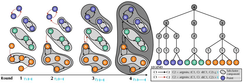
Figure 1: The Sub-Clustering Component Algorithm. We illustrate SCC on a small dataset. The formation of sub-clusters is shown with black arrows for pairs of points satisfying Def. 3. The direction indicates indicates the nearest neighbor relationship (Def. 3, condition 2). Red edges indicate the nearest neighbor relationships that are above the distance thresholds. The grey circles indicate the sub-cluster components created in that round. Best viewed in color.

2.2 Proposed Approach

SCC works in a best-first manner: determining which points should belong together in clusters in a sequence of rounds. The sequence of rounds begins with the decisions that are “easy to make” (e.g., points that are clearly in the same cluster) and prolongs the later, more difficult decisions until these confident decisions have been well established. SCC starts by putting each point into its own separate cluster. Then in each round, we merge together groups of clusters from the previous round that satisfy a given certain “condition”. The merging operation continues, until there are no pairs of clusters remaining to be merged. Each round of our algorithm produces a partition (flat clustering) of the dataset at a different granularity and the collection of rounds together forms a hierarchical clustering (with non-parametric branching factor).

Let $\mathbf{\mathbb{S}}^{(i)}$ be the partition produced after round $i$ and the partition at the starting round be $\mathbf{\mathbb{S}}^{(0)}=\{\{x\}|x\in\bm{X}\}$. Let a sub-cluster refer to a member a partition, i.e. $C\in\mathbf{\mathbb{S}}^{(i)}$. Let $\tau_{1},\dots\tau_{L}$ be a series of $L$ predefined increasing thresholds, given as hyperparameters to the algorithm. To specify the “condition" under which we merge sub-clusters in each round, we define sub-cluster component as:

Definition 3.

[Sub-cluster Component] Two sub-clusters $C_{j},C_{k}\in\mathbf{\mathbb{S}}$ are defined to be part of the same sub-cluster component according to a threshold $\tau$ and linkage $d:\mathcal{P}({\bm{X}})\times\mathcal{P}({\bm{X}})\rightarrow\mathbb{R}^{+}$, denoted $\textsc{Ch}_{d}(C_{j},C_{k},\tau,\mathbf{\mathbb{S}})=1$, if there exists a path $P\subseteq\mathbf{\mathbb{S}}$ defined as $\{C_{j}=C_{s_{0}},C_{s_{1}},C_{s_{2}},\ldots C_{s_{R-1}},C_{s_{R}}=C_{k}\}$, where each the following two conditions are met:

1. $d(C_{s_{r}},C_{s_{r-1}})\leq\tau\;\text{ for }\,0\leq r\leq R$, and

2. either $C_{s_{r-1}}=\mathop{\mathrm{argmin}}_{C\in\mathbf{\mathbb{S}}}d(C_{s_{r}},C)$ and/or
   $C_{s_{r}}=\mathop{\mathrm{argmin}}_{C\in\mathbf{\mathbb{S}}}d(C_{s_{r-1}},C)$.

Inference at round $i$ works by merging the sub-clusters in round $i-1$ that are in the same sub-cluster component. Computationally, the construction of sub-cluster components can be thought of as the connected components of a graph with nodes as the sub-clusters from the previous round and edges between pairs of nodes that are nearest neighbors and are less that $\tau$ from one-another.

We define, $\textsc{SC}_{d}(C_{j},\mathbf{\mathbb{S}},\tau)$, as the union of all sub-clusters in $\mathbf{\mathbb{S}}$ that are within the sub-cluster component of $C_{j}$, i.e.,

$$\textsc{SC}_{d}(C_{j},\mathbf{\mathbb{S}},\tau)\vcentcolon=\bigcup\limits_{\begin{subarray}{c}C\in\mathbf{\mathbb{S}},\\ \textsc{Ch}_{d}(C_{j},C,\tau,\mathbf{\mathbb{S}})=1\end{subarray}}C$$ (1)

Thus, $\textsc{SC}_{d}(C_{j},\mathbf{\mathbb{S}}^{(i-1)},\tau^{(i)})$ is a new cluster, created by taking a union of all clusters from round $i-1$ that are in the sub-cluster component of $C_{j}$. We create $\mathbf{\mathbb{S}}^{(i)}$, flat partition at round $i$, as the set of all of these newly found clusters:

$$\mathbf{\mathbb{S}}^{(i)}\vcentcolon=\{\textsc{SC}_{d}(C,\mathbf{\mathbb{S}}^{(i-1)},\tau^{(i)})\,|\,C\in\mathbf{\mathbb{S}}^{(i-1)}\}$$ (2)

We refer to our algorithm as the Sub-Cluster Component algorithm (SCC). Alg. 1 gives pseudocode for SCC. We only increment the threshold if no clusters are merged in the previous round i.e. $\mathbf{\mathbb{S}}^{(i-1)}=\mathbf{\mathbb{S}}^{(i)}$. The sub-cluster component in a particular round can be found efficiently using a connected components algorithm [10]. Any of the rounds can be used as a predicted flat clustering. A hierarchical clustering is given by $\bigcup\textsc{SCC}(\bm{X},d,\{\tau_{1},\dots,\tau_{L}\})$, the union of the sub-clusters produced by all rounds. Figure 1 provides an illustration of the SCC algorithm and the sub-cluster formation.

Algorithm 1 Sub-Cluster Component Alg. (SCC)

1:Input: $\bm{X}$: dataset , $d$: set dissimilarity, $\{\tau_{1},\ldots,\tau_{L}\}$: a set of thresholds in increasing order

2:Output: $(\mathbf{\mathbb{S}}^{(0)},\mathbf{\mathbb{S}}^{(1)},\ldots)$: One flat partition per round

3:$\mathbf{\mathbb{S}}^{(0)}\leftarrow\{\{x\}\ |\ x\in\bm{X}\}$

4:$\textsf{idx}\leftarrow 1$, $i\leftarrow 1$

5:while $\textsf{idx}<L$ do

6:     Set $\textsc{SC}_{d}(C_{i},\mathbf{\mathbb{S}}^{(i-1)},\tau^{(i)})$, $\forall C_{i}\in\mathbf{\mathbb{S}}^{(i-1)}$, (Eq. 1)

7:     Set $\mathbf{\mathbb{S}}^{(i)}$ (Eq. 2)

8:     $\textsf{idx}\leftarrow\textsf{idx}+\mathbb{I}[\mathbf{\mathbb{S}}^{(i)}=\mathbf{\mathbb{S}}^{(i-1)}]$

9:     $i\leftarrow i+\mathbb{I}[\mathbf{\mathbb{S}}^{(i)}\neq\mathbf{\mathbb{S}}^{(i-1)}]$

10:     $\tau^{(i)}\leftarrow\tau_{\textsf{idx}}$

11:return $(\mathbf{\mathbb{S}}^{(0)},\ldots,\mathbf{\mathbb{S}}^{(i-1)})$

3 Analysis

SCC is a simple, intuitive algorithm for clustering that has a number of desirable theoretical properties. We provide theoretical analysis of SCC used for both flat and hierarchical clustering. We analyze the separability conditions under which SCC recovers the target clustering and connect these results to the DP-Means objective as well as hierarchical clustering evaluation measures. Lastly, we show that in the limit of number of rounds our method will produce the same tree structure as agglomerative clustering.

3.1 Recovering Target Clustering

Separability assumptions in clustering provide a mechanism to understand whether or not an algorithm effectively and efficiently recovers cluster structure under “reasonable” conditions. If we can define a center for a cluster of points, then we can define $\delta$-separability, which expresses a ratio between the center-to-center dissimilarities and the point which is farthest from its assigned center.

Assumption 1.

($\delta$-Separability [41]) We say that the input data $\bm{X}$ satisfies $\delta-$separation, with respect to some target clustering $\mathbf{\mathbb{S}}^{\star}=\{C_{1},C_{2},\ldots,C_{k}\}$ if there exists centers $c_{1}^{\star},\ldots c_{k}^{\star}$ such that for all $i\neq j$ $||c^{\star}_{i}-c^{\star}_{j}||\geq\delta\cdot R$ where $R:=\max_{l\in[k]}\max_{x\in C_{l}}||x-c_{l}^{\star}||$ .

Each round of SCC produces a flat clustering of a dataset $\bm{X}$. We will show that if $\bm{X}$ satisfies the above $\delta$-separability assumptions, one of the rounds of SCC will in fact be equal to the target clustering for the dataset, $\mathbf{\mathbb{S}}^{\star}$, corresponding to the separated clusters. Formally, we make the statement:

Theorem 1.

Suppose the dataset $\bm{X}$ satisfies the $\delta$-separability assumption with respect to the target clustering $\mathbf{\mathbb{S}}^{\star}=\{C^{\star}_{1},\dots,C^{\star}_{k}\}$ for $\delta\geq\gamma$. $SCC(\bm{X},d,\{\tau_{0},\dots,\tau_{L}\})$ is set of partitions produced by SCC (Alg. 1) with $d(\cdot,\cdot)$ as average linkage and geometrically increasing thresholds i.e. $\tau_{i}=2^{i}\cdot\tau_{0}$. The target clustering is equal to one of the clustering produced by one round of SCC, $\mathbf{\mathbb{S}}^{\star}\in SCC(\bm{X},d,\{\tau_{0},\dots,\tau_{L}\})$, where $\gamma=6$ for all metrics and $\gamma=30$ for the $\ell_{2}^{2}$ distance and $\tau_{0}\leq\min_{x,x^{\prime}\in\bm{X}^{2}}||x-x^{\prime}||$.

The proof of Theorem 1 is given in the supplemental material (§A.1). Intuitively, we prove that, for the aforementioned bounds on within/across cluster distances, a geometric series will include a threshold that is larger than largest within cluster distance and smaller than the closest across cluster distance between any two sub-clusters. Having such a threshold $\tau^{\star}$, we will have a round $i$ with a flat clustering, $\mathbf{\mathbb{S}}^{(i)}$, equal to the target clustering $\mathbf{\mathbb{S}}^{\star}$, $\mathbf{\mathbb{S}}^{(i)}=\mathbf{\mathbb{S}}^{\star}$.

We also consider a more general class of separable data, model-based separation [45], which specifies when a particular linkage function “separates” a dataset. In model-based separation, we view the dataset $\bm{X}$ as the nodes in an undirected graph with latent (unobserved) edges. The edges of this graph provide connected components, which correspond exactly to a target clustering $\mathbf{\mathbb{S}}^{\star}$.

Assumption 2.

(Model-based Separation [45]) Let $G=(\bm{X},E)$ be a graph. Let the function $d:\mathcal{P}(\bm{X})\times\mathcal{P}(\bm{X})\rightarrow\mathbb{R}$ be a linkage function that computes the similarity of two groups of vertices and let $g:\mathcal{P}(\bm{X})\times\mathcal{P}(\bm{X})\rightarrow\{0,1\}$ be a function that returns 1 if the union of its arguments is a connected subgraph of $G$. Dataset $\bm{X}$ is model-based separated with respect to $f$ if:

$$\forall C_{0},\ C_{1},\ C_{2}\subseteq\bm{X},\ g(C_{0},C_{1})>g(C_{0},C_{2})\implies d(C_{0},C_{1})<d(C_{0},C_{2}).$$

The target partition, $\mathbf{\mathbb{S}}^{\star}$, which is model-based separated, corresponds to connected components in $G$.

We show that for datasets that are model separated our algorithm will contain the target clustering, i.e.,

Proposition 1.

Given a dataset $\bm{X}$ and a symmetric injective linkage function $f$ s.t. $\bm{X}$ is model-based separated with respect to $f$, let $\mathbf{\mathbb{S}}^{\star}$ be the target partition corresponding to the separated data. There exists a $\tau_{1},\dots,\tau_{L}$ such that the hierarchical clustering $\bigcup\textsc{SCC}(\bm{X},\{\tau_{1},\dots,\tau_{L}\},d)$ discovered by SCC contains the target partition $\mathbf{\mathbb{S}}^{\star}$.

Please refer to the supplemental material for the proof (§A.2).

3.2 Relation to Nonparametric Clustering

Next, we analyze the performance of our algorithm with respect to nonparametric, flat clustering cost functions. Nonparametric clustering, where the number of clusters is not known a priori and must be inferred from the data, is useful for many clustering applications [1, 32, 40]. DP-means [32, 40, 11] is an example of a widely used nonparametric cost function, that is obtained from the small variance asymptotics of Dirichlet Process mixture models.

Definition 4.

[DP-Means [32]] Given a dataset $\bm{X}$, a partition $\mathbf{\mathbb{S}}=\{C_{1},\dots,C_{K}\}$, such that cluster $C_{l}$ has center $c_{l}$ and hyperparameter $\lambda$, the DP-Means objective is:

$$DP(\bm{X},\lambda,\mathbf{\mathbb{S}})=\sum_{C_{l}\in\mathbf{\mathbb{S}}}\sum_{x\in C_{l}}||x-c_{l}||^{2}+\lambda|\mathbf{\mathbb{S}}|.$$ (3)

Given a dataset $\bm{X}$ and hyperparameter $\lambda$, clustering according to DP-Means seeks to find: $\mathop{\mathrm{argmin}}_{\mathbf{\mathbb{S}},\textbf{c}}DP(\bm{X},\lambda,\mathbf{\mathbb{S}})$ where c are the centers for each cluster in $\mathbf{\mathbb{S}}$.

We show that SCC yields a constant factor approximation to DP-Means solution under $\delta$-separation (Assumption 1).

Theorem 2.

Suppose the dataset $\bm{X}$ satisfies the $\delta$-separability assumption with respect to the target clustering $\mathbf{\mathbb{S}}^{\star}=\{C^{\star}_{1},\dots,C^{\star}_{k}\}$ for $\delta\geq\gamma$. $SCC(\bm{X},d,\{\tau_{0},\dots,\tau_{L}\})$ is set of partitions produced by SCC with $d(\cdot,\cdot)$ as the average distance between points and geometrically increasing thresholds i.e. $\tau_{i}=2^{i}\cdot\tau_{0}$. $SCC(\bm{X},d,\{\tau_{0},\dots,\tau_{L}\})$ contains a $2$-approximation solution to the DP-Means objective.

See Appendix §A.1 for the proof. The two primary steps are: (1) Using theorem 1 and show that SCC can find optimal solution to the facility location problem and (2) show that this solution is a constant factor approximation of the DP-means solution.

Our analysis of SCC as an approximation algorithm for DP-Means shows the first connection of hierarchical bottom up clustering to non-parametric flat clustering objectives such as DP-means. This theoretical connection is also empirically useful as SCC achieves SOTA for the DP-means objective (§4.3).

3.3 Hierarchical Clustering Analysis

SCC is reminiscent of hierarchical agglomerative clustering (HAC), which, in each round, merges the two subtrees with minimum distance according to the linkage function. In the following statement, we show that there exists a sequence of thresholds $\tau_{0},\dots,\tau_{L}$, for which SCC will produce exactly the same tree structure as HAC. To formally make this statement, we need to make the additional assumption that the linkage function is both injective (so as there are no ties in the ordering of mergers) and reducible.

Proposition 2.

Let $d:\mathcal{P}({\bm{X}})\times\mathcal{P}({\bm{X}})\rightarrow\mathbb{R}^{+}$ be a linkage function that is symmetric and injective, $C_{1},C_{2},C_{3},C_{4}\subset\bm{X},\ d(C_{1},C_{2})=d(C_{3},C_{4})\iff(C_{1}=C_{3}\wedge C_{2}=C_{4})\vee(C_{1}=C_{4}\wedge C_{2}=C_{3})$. Let ${\mathcal{T}}$ be the tree formed by HAC and let $d$ also satisfy reducibility, $\forall C,C^{\prime},C^{\prime\prime}\in{\mathcal{T}},\ f(C,C^{\prime})\leq\min\{d(C,C^{\prime\prime}),d(C^{\prime},C^{\prime\prime})\}\implies\min\{d(C,C^{\prime\prime}),d(C^{\prime},C^{\prime\prime})\}\leq d(C\cup C^{\prime},C^{\prime\prime})$ then there exists a sequence of threshold $t_{1},\dots,t_{r}$ such that the tree formed by SCC, i.e., $\bigcup\textsc{SCC}(\bm{X},f,\{\tau_{1},\dots,\tau_{r}\})$, is the same as ${\mathcal{T}}$.

Proof. Each node in the HAC tree, $C\in{\mathcal{T}}$, has an associated linkage function score, denoted (with abuse of notation) as $d(C)$. We define the threshold-based rounds for SCC such that $t_{1},\dots,t_{r}$ to be the values, $\{d(C)+\epsilon|C\in{\mathcal{T}}\}$ sorted in ascending order. Because $f$ is reducible and injective, there is a unique pair of nodes that will be merged in each round. This pair will correspond exactly to the pair that is merged by HAC in the corresponding round. It follows that the resulting tree structures will be identical. $\square$

The connection between SCC and agglomerative clustering is used to prove Proposition 1. We note that SCC produces non-binary tree structures. And so SCC is not meant to directly approximate the binary tree produced by HAC, nor is it not well suited for objectives such as Dasgupta’s cost [18].

3.4 Time Analysis

Worst Case

Building the sub-cluster components in each round is achieved by first finding the 1-nearest neighbor of each point that is less than the given round threshold. Then forming weakly connected components in the graph with edges of the aforementioned 1-nearest neighbor relationships. For a given round, let $O(T)$ be the time required to build a 1-nearest neighbor graph over the sub-clusters of a round. Cover Trees [8] allow this to be done in $O(c^{12}N\log N)$ for $N$ elements where $c$ is the expansion constant. Let $O(S)$ be the time required to run connected components. Since we are finding the connected components of a graph with $N$ nodes and at most $N$ edges, a worst case running time of connected components is $O(N)$. We note that each of the one nearest neighbor graph and the connected components algorithm are highly parallelizable in a map-reduce framework. In the worst case, SCC requires $2*(N-1)$ rounds (merging one pair of elements per round, multiplicative factor due to determining when to advance idx in Algorithm 1). In general this is a $O(N(T+S))$ running time. We find that using a fixed number of rounds and simply advancing the threshold in each round experimentally works well.

Sparse Graphs

To speed up computation, we can pre-compute a $k$ nearest-neighbor graph over the dataset. Once such a graph is constructed computing the 1-nearest neighbor of each node can be an $O(k)$ operation for many linkage functions (such as average, single, complete). We can use the sparse $k$ nearest-neighbor graph to compute “top-k” approximation of the linkage functions. For instance, to compute the average linkage between two clusters of points according to the $k$-nearest-neighbor graph, we can define the distance between any two points that do not share an edge in the sparse $k$ nearest neighbor graph to be a fixed constant (e.g., 4 in the case of $\ell_{2}^{2}$ or 0 in the case similarities).

4 Experiments

We empirically validate the effectiveness of SCC. Paralleling our theoretical contributions, we analyze the method both as hierarchical clustering approach as well as a flat clustering method and DP-Means approximation algorithm. Analysis on a variety of publicly available clustering benchmarks demonstrates that SCC:

• Recovers more accurate hierarchical clustering than state-of-the-art methods (§4.1).

• Produces high quality flat partitions of the data (§4.2).

• Produces lower DP-means cost solutions (§4.3).

Lastly, to demonstrate the scalability of SCC we evaluate on 30 billion point web-scale dataset (§5).

4.1 Hierarchical Clustering

Datasets: We evaluate the SCC and competing methods on the following publicly available clustering benchmark datasets as in [36] (Table 1): CovType - forest cover types; Speaker - i-vector speaker recordings, ground truth clusters refer each unique speaker [27]; ALOI - 3D rendering of objects, ground truth clusters refer to each object type [24]; ILSVRC (Sm.) (50K subset) and ILSVRC (Lg.) (1.2M Images) images from the ImageNet ILSVRC 2012 dataset [50] with vector representations of images from the last layer of the Inception neural network.

Methods We analyze the performance of SCC compared to state-of-the-art hierarchical clustering algorithms: Affinity [6] - a distributed minimum spanning tree approach based on Borůvka’s algorithm [10]; Perch [36] - an online hierarchical clustering algorithm that creates trees one point at a time by adding points next to their nearest neighbor and perform local tree re-arrangements in the form of rotations; Grinch [45] - similar to Perch this is an online tree building method, this work uses a grafting subroutine in addition to rotations. The graft subroutine allows for more global re-arrangements of the tree structure; gHHC [46] - a gradient-based hierarchical clustering method that uses a continuous tree representation in the unit ball; hierarchical K-Means (HKM) - the top down divisive algorithm; hierarchical agglomerative clustering (HAC) - the classic bottom up agglomerative approach; Birch [59] - a classic top-down hierarchical clustering method; HDBSCAN [12] - the hierarchical extension of the classic DBSCAN algorithm. For Perch, Grinch, HKM, Birch, gHHC we report results from previous work [36, 46, 45]. Cosine similarity is meaningful for each of the datasets. For all methods that use a linkage function, we use average linkage which was shown to be effective [45].

	CovType	ILSVRC	ALOI	Spkr.	ILSVRC
		(Sm.)			(Lg.)
$|\mathbf{\mathbb{S}}^{\star}|$	7	1000	1000	4958	1000
$|\bm{X}|$	500K	50K	108K	36.5K	1.3M
dim.	54	2048	128	6388	2048
BIRCH	0.44	0.26	0.32	0.22	0.11
Perch	0.448	0.531	0.445	0.372	0.207
HAC	-	0.641	0.524	0.518	-
Grinch	0.430	0.557	0.504	0.48	-
HKM	0.44	0.12	0.44	0.12	0.11
gHHC	0.444	0.381	0.462	-	0.367
HDBSCAN	0.473	0.414	0.599	0.396	-
Affinity	0.433	0.587	0.478	0.424	0.601
SCC	0.433	0.644	0.619	0.528	0.614

Table 1: Dendrogram Purity results on benchmark datasets. gHHC did not produce meaningful results on Speaker and Grinch and HDBSCAN did not scale to ILSVRC (Lg.).

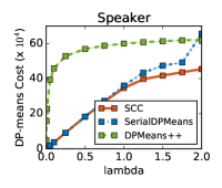
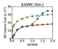
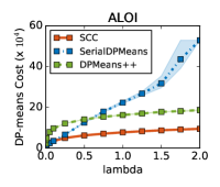
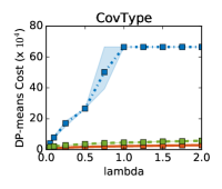
Figure 2: DP-Means Cost for the solutions found with a variety of methods for a range of $\lambda$ values from close to 0 to 2. SCC produces lower cost solutions for different values of $\lambda$ as compared to the other methods.

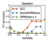
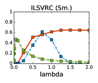
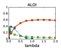
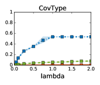
Figure 3: Pairwise F1 Evaluation. As each algorithm depends on $\lambda$ in a different way, the settings of $\lambda$ resulting in the best performance might differ between methods. We plot the performance of each method for each value of $\lambda$. When considering the best F1 achieved by each method for some value of $\lambda$, SCC is the top performing method on 4 of 5 datasets.

Since the datasets use cosine similarity, for SCC, we use a geometric progression of thresholds for SCC based on the bounds of cosine similarity (switching the sign of threshold condition), which we approximate with minimum (0.001) to maximum (1.0) with 200 thresholds for the algorithm. We use the sparsified nearest neighbor graph approach with $k$=25 neighbors using we ScaNN [29].

Since each dataset has ground truth flat clusters, we evaluate the quality of hierarchy using dendrogram purity as in previous work [31, 36, 45]. Dendrogram purity is the average, over all pairs of points from the same ground truth cluster, of the purity of the least common ancestor of the pair. We hypothesize that SCC’s improvement over Affinity clustering comes from its use of round-based thresholds to reduce the overmerging of clusters.

As seen in Table 2, we observe that SCC achieves the highest dendrogram purity on all datasets except CovType. Notably, both SCC and Affinity clustering scale much better to the largest 1.2M image dataset, with both methods having no degradation in performance from the 50K subset to the larger 1.2M point dataset.

We analyze the decision to use geometric progression for thresholds as compared to linear ones in Figure 5. We observe that SCC performs slightly better with geometric sequences compared to linear ones. We also observe that SCC requires only a few more rounds than Affinity to begin to achieve high quality results and that the performance saturates after a few hundred rounds.

Comparison to HAC We sample datasets of varying sizes from a Dirichlet Process Mixture Model. Figure 4 reports the running time and dendrogram purity as a function of the dataset size. We report SCC results with 200 rounds. We observe that while the time complexity of HAC grows quadratically, SCC remains much more constant. Despite being much more efficient than HAC we observe that SCC produces trees with comparable dendrogram purity.

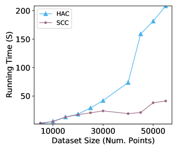
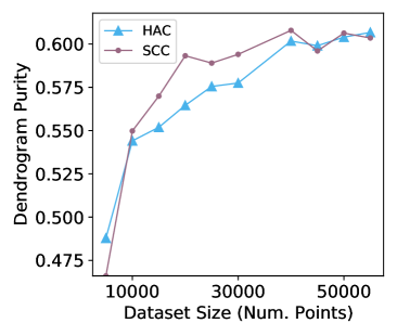
Figure 4: Comparison to HAC: We report running time and Dendrogram Purity of SCC compared to HAC, on a synthetic dataset.

4.2 Flat Clustering

	CovType	ILSVRC	ALOI	Spkr.	ILSVRC
		(Sm.)			(Lg.)
Perch	0.230	0.543	0.442	0.318	0.257
K-Means	0.245	0.605	0.408	0.322	0.562
Affinity	0.536	0.632	0.439	0.299	0.641
SCC	0.536	0.609	0.567	0.493	0.602
Affinity (best F1)	0.536	0.632	0.465	0.314	0.641
SCC (best F1)	0.536	0.654	0.605	0.526	0.664

Table 2: Pairwise F1 results on benchmark datasets.

In this section, we empirically evaluate SCC against state-of-the-art approaches in terms of pairwise F1 of flat clusters discovered. We use the same experimental setting as in previous works [36]. In this experiment, we use the ground truth number of clusters when selecting a flat clustering. We select the round of SCC which produced the closest number of clusters to the ground truth and report the flat clustering performance of that round. We do the same for baseline methods. We evaluate the quality of the flat clusterings using the pairwise F1 metric [36, 44], for which precision is defined as $\textsf{Prec}=\frac{|\mathcal{P}^{*}\cap\hat{\mathcal{P}}|}{|\hat{\mathcal{P}}|}$, and recall as $\textsf{Rec}=\frac{|\mathcal{P}^{*}\cap\hat{\mathcal{P}}|}{|{\mathcal{P}^{*}}|}$, where $\mathcal{P}^{*}$ is all pairs of points that are assigned to the same cluster according to the ground truth $\mathbf{\mathbb{S}}^{*}$ and $\hat{\mathcal{P}}$ is similarly defined for the predicted clustering $\hat{\mathbf{\mathbb{S}}}$: $\mathcal{P}^{*}=\{(x_{i},x_{j})\ |\ \ x_{i},x_{j}\in\bm{X},\ \exists\ C^{*}\in\mathbf{\mathbb{S}}^{*}\text{ s.t. }\{x_{i},x_{j}\}\subseteq C^{*}\}$ and $\hat{\mathcal{P}}=\{(x_{i},x_{j})\ |\ x_{i},x_{j}\in\bm{X},\ \exists\ C\in\hat{\mathbf{\mathbb{S}}}\text{ s.t. }\{x_{i},x_{j}\}\subseteq C\}$

Table 2 gives the F1 performance for each method on each of the datasets used in the hierarchical clustering experiments. We observe that both SCC and Affinity outperform the previous state-of-the-art results reported by [36]. SCC is the best performing method on Speaker and ALOI and is competitive with Affinity on the remaining datasets. We report the best F1 achieved in any round of our algorithm and Affinity, which is the next best performing method. SCC’s best F1 is better than Affinity’s.

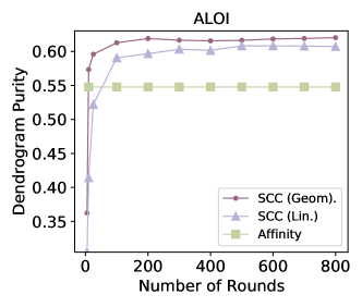
Figure 5: Number of Round $\&$ Kinds of Thresholds. We report SCC’s performance with both a geometric progression of thresholds and a linear progression of thresholds. We also report Affinity’s performance, which converges in about five rounds. Recall that HAC would require number of rounds equal to number of points (much more than 800).

4.3 Approximation of DP-Means Objective

Our analysis section (§3.2) showed that SCC is a DP-Means approximation algorithm. In this section, we empirically evaluate these claims. We measure the quality of the clustering discovered by our algorithm in terms of the DP-Means objective.

We compare SCC to the following state-of-the-art algorithms for obtaining solutions to the DP-means objective: SerialDPMeans, the classic iterative optimization algorithm for DP-Means [11, 32, 40, 49], in which data point is added to a cluster if it is within $\lambda$ of that cluster center and otherwise starts a new cluster; DPMeans$++$ [3] an initialization-only method which performs a K-Means$++$ [2] style sampling procedure. For each method, we record the assignment of points to clusters given by inference. We use this assignment of points to flat clusters to produce a DP-Means cost. We perform our analysis on the aforementioned clustering benchmarks.

Figure 2 shows the DP-Means objective as a function of the value of the parameter $\lambda$. Figure 3 shows the corresponding F1 performance for different values of $\lambda$ (0.001, 0.005, 0.01, 0.05, 0.1, 0.25, 0.5, 0.75, 1.0, 1.25, 1.5, 1.75, 2.0). We report the min/max/average performance over multiple runs of the SerialDPMeans and DPMeans$++$ algorithms with different random seeds. Here, each method uses normalized $\ell_{2}^{2}$ distance as the dissimilarity measure. SCC uses thresholds $0.001$ to $4$ with a geometric progression.

For each value of $\lambda$, SCC achieves the lowest DP-Means cost, which we hypothesize is due to SCC discovering optimal clustering independently of $\lambda$ via multiple alternative partitions in the tree. As each algorithm uses the value of $\lambda$ differently, the value of $\lambda$ that results in the best F1 score on the dataset could be quite different for each method and for each dataset. If we consider the best F1 value achieved, SCC is usually one of the best performing methods. On CovType, SerialDPMeans performs best. but F1 does not seem meaningful on CovType as we observed the highest F1 value (0.536) with all points in a single cluster. See Appendix §B for ILSVRC (Lg.) results and comparison to LowrankALBCD [57].

5 Application: Large Scale Clustering of Web Queries

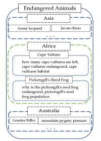
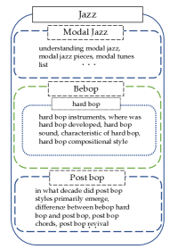
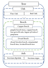
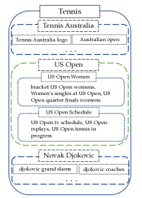
Figure 6: Hierarchy inferred on 30 billion user queries using SCC. We represent the hierarchy using rectangular boxes. The root with header is represented by the outer rectangular box (solid line). The second level of the hierarchy, with header, is shown in dashed ($-\ -$) rectangle withing the outer box. Finally the third level from the root is shown as the inner most dotted ($...$) rectangle. Plain text within each of the dotted rectangle are the top queries that belong to that cluster. For example, Endangered Animals, is the root of the left most hierarchy, Endangered Animals in Africa is a sub-cluster and pickergill’s reed frog is the lowest level cluster containing queries such as why is the pickergill’s reed frog endangered.

We investigate the use of SCC for clustering web queries. We run our proposed clustering approach and Affinity clustering on a dataset of a random sample of 30 billion queries. To the best of our knowledge this is one of the largest evaluations of any clustering algorithm. Due to the massive size of the data, we limit our evaluation to the two most highly performing methods, SCC and Affinity clustering. Distance computation between queries during algorithm execution are sped-up using hashing techniques to avoid the $N^{2}$ pairwise dissimilarity bottleneck (for both SCC and Affinity). Queries are represented using a set of proprietary features comprising lexical and behavioral signals among others. We extract manually a fine-grained level of flat clusterings and compared the clustering quality of the flat clusterings discovered by both algorithms.

Human Evaluation: To evaluate the quality of flat clusters discovered by SCC, we conducted an empirical evaluation with human annotators. We asked them to rate $\sim 1200$ randomly sampled clusters from -1 (incoherent) to +1 (coherent). For example, a annotator might receive a head query of home improvement and a tail query of lowes near me from the same cluster. The annotator then rates each of these pairs from -1 (incoherent) to +1 (coherent). We report the aggregated results in Figure 7. We found that the annotators labeled 6.0% of Affinity clustering’s clusters and only 2.7% of SCC clusters as incoherent. The annotators labeled 55.8% of Affinity’s clusters and 65.7% of SCC clusters as coherent. We hope this demonstrates the cogency of the clusters found by SCC.

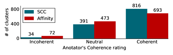
Figure 7: Human evaluation of clusters generated by SCC and Affinity

Qualitative Evaluation: In Table 3, we show the clusters discovered by both SCC and Affinity that contain the query Green Velvet (the house/techno music artist). We observe that SCC’s cluster is considerably more precise and on topic. Table 4, shows additional examples. We find the clusters to be precise and coherent. The algorithm discovers a clustering related to tennis strategies, which contains meaningful queries such as baseline tactics and tennis strategy angles. We investigate the hierarchical structure in Figure 6. We discover meaningful clusters at multiple granularities with the tree structure indicating meaningful relationships between topics. For instance, we discover subgenres of jazz such as bebop and modal jazz. We further discover that hard bop is a subgenre of bebop.

Affinity Clustering	SCC
green velvet live	green velvet mix
green velvet talking	dj green velvet
kestra financial businesswire	tomorrowland green velvet
tomorrow land green velvet	green velvet 2015
dj green hair	green velvet music
rinvelt & david kestra businesswire	green velvet dj set

Table 3: SCC and Affinity Clustering for clusters corresponding to green velvet on the 30 billion query dataset.

Tea Recipes	Electric Piano	Tennis Strategy
tea drinks	digital piano price	playing strategies in tennis
tea recipes	electric piano sale	understanding tennis tactics
fancy tea recipes	electric piano small	baseline tactics.
black tea flavors	best digital piano ebay	tennis strategy angles

Table 4: Fine-grained Query Clusters Discovered by SCC

6 Related Work

Parallel and distributed approaches for hierarchical clustering have been considered by previous work [48, 33, 6, 56, 51]. Yaroslavtsev and Vadapalli [56] use a graph sparsification approach along with parallel minimum spanning tree approach to achieve provably good approximate minimum spanning trees. Other work has proposed to achieve scalability by building hierarchical clusterings in an online, incremental, or streaming manner [59, 38, 36, 45]. BIRCH, one of the most widely used algorithms, builds a tree in a top down fashion splitting nodes under a condition on the mean/variance of the points assigned to a node. PERCH [36] and GRINCH [45] add points next to the nearest neighbor node in the tree structure and perform tree re-arrangements. Kranen et al. [38] build an adaptive index structure for streaming data with allows for recency weighting.

Our work is closely related to the tree-based clustering methods proposed by Balcan et al. [4, 5]. These methods also build a tree structure in a bottom up manner using round-specific thresholds to determine the mergers. These methods in fact recover clusterings under more flexible separation conditions than the one used in this paper. However, the linkage function computation used is more computationally expensive than the one used in this paper. We show an empirical comparison of this to SCC in Appendix §B .

While this paper has focused on linkage-based hierarchical clustering in general, density-based clustering algorithms like DBSCAN [22] correspond to specific linkage functions. There have been several hierarchical variants of these approaches proposed including, most recently HDBSCAN^∗ [12]. There are other related density and spanning-tree-based approaches [13, 62].

Other work has use techniques to reduce the number of distance computations required to perform hierarchical clustering [21, 39]. Krishnamurthy et al. [39] uses only $O(n\log^{2}(n))$ distance computations by repeatedly running a flat clustering algorithm on small subsets of the data to discover the children of each node in a top-down way. Other work uses nearest neighbor graph sparsification to reduce the complexity of algorithms [58].

A variety of objective functions have been proposed for hierarchical clustering. Some work has used integer linear programming to perform hierarchical agglomerative clustering [25]. Notably, Dasgupta’s cost function [18] has been widely studied, including its connections to agglomerative clustering [47, 14].

7 Conclusion

We introduce the Sub-Cluster Component algorithm (SCC) for scalable hierarchical as well as flat clustering. SCC uses an agglomerative, round-based, approach in which a series of increasing distance thresholds are used to determine which sub-clusters can be merged in a given round. We provide a theoretical analysis of SCC under well studied separability assumptions and relate it to the non-parametric DP-means objective. We perform a comprehensive empirical analysis of SCC demonstrating its proficiency over state-of-the-art clustering algorithms on benchmark clustering datasets. We further provide an analysis of the method with respect to the DP-means objective. Finally, we demonstrate the scalability of SCC by running on an industrial web-scale dataset of 30B user queries. We evaluate clustering quality on this web-scale dataset with human annotations that indicate that the clusters produced by SCC are more coherent than state-of-the-art methods.

Scalable Hierarchical Agglomerative Clustering – Appendix

Appendix A Proofs

A.1 Proof of Theorem 1

Here we show a proof for the $\ell_{2}^{2}$ case, the $\ell_{2}$ case follows the same proof but uses the triangle inequality instead of the relaxed triangle inequality. Recall the assumption of $\delta$-separability (Assumption 1) in which the maximum distance from any point to its true center is defined as $R:=\max_{i\in[k]}\max_{x\in C^{*}_{i}}\|x-C^{*}_{i}\|_{2}^{2}$. We make the additional assumption that the threshold of the first round, $\tau_{0}$, is less than $R$, i.e., $\tau_{0}<R$.

The algorithm begins with $\mathbf{\mathbb{S}}^{(0)}$ set to be the shattered partition, with each data point in its own cluster, $\mathbf{\mathbb{S}}^{(0)}=\{\{x\}|x\in\bm{X}\}$.

We want to show that some round, $r^{\star}$ with threshold $\tau_{r}$ produces the ground truth partition, $\mathbf{\mathbb{S}}^{(r^{\star})}=\mathbf{\mathbb{S}}^{*}=\{C_{1}^{*},\dots,C_{k}^{*}\}$. We will show by induction that for each round prior $r^{\prime}\leq r^{\star}$ that the clustering $\mathbf{\mathbb{S}}^{(r^{\prime})}$ is pure, i.e. $\forall C\in\mathbf{\mathbb{S}}^{(r^{\prime})},\ \exists C^{*}\in\mathbf{\mathbb{S}}^{*}\ C\subseteq C^{*}$ (equality will be for round $r^{\star}$). We will show the round $r^{\star}$ with $\mathbf{\mathbb{S}}^{(r^{\star})}=\mathbf{\mathbb{S}}^{*}$ must exist.

In our inductive hypothesis, we assume that for rounds before and including $\tau_{r}$, we have pure sub-clusters such that $X,X^{\prime}\subseteq C^{*}_{i}$, which are disjoint, $X\cap X^{\prime}=\emptyset$, and $Y\subseteq C^{*}_{j}$ for $i\neq j$ ($\mathbf{\mathbb{S}}^{(0)}$ by definition has pure sub-clusters). We want to show: every such $X$ and $X^{\prime}$ must form a sub-cluster component without any such $Y$. In this way, we ensure that $C^{*}_{i}$ exists as a pure cluster in some round. Using the relaxed triangle inequality [28] for $\ell_{2}^{2}$, we have:

$$\vspace{-1mm}\|c_{i}^{*}-c_{j}^{*}\|_{2}^{2} \leq 3\left(\frac{1}{|X||Y|}\sum_{x\in X}\sum_{y\in Y}\|c_{i}^{*}-x\|_{2}^{2}+\|x-y\|_{2}^{2}+\|y-c_{j}^{*}\|_{2}^{2}\right)$$

$$\|c_{i}^{*}-c_{j}^{*}\|_{2}^{2} \leq 3\left(\frac{1}{|X|}\sum_{x\in X}\|c_{i}^{*}-x\|_{2}^{2}+\frac{1}{|X||Y|}\sum_{x\in X}\sum_{y\in Y}\|x-y\|_{2}^{2}+\frac{1}{|Y|}\sum_{y\in Y}\|y-c_{j}^{*}\|_{2}^{2}\right)$$

$$\vspace{-2mm}\frac{1}{3}\|c_{i}^{*}-c_{j}^{*}\|_{2}^{2}-\frac{1}{|X|}\sum_{x\in X}\|c_{i}^{*}-x\|_{2}^{2}-\frac{1}{|Y|}\sum_{y\in Y}\|y-c_{j}^{*}\|_{2}^{2}\leq\frac{1}{|X||Y|}\sum_{x\in X}\sum_{y\in Y}\|x-y\|_{2}^{2}$$

Since $\|c_{i}^{*}-c_{j}^{*}\|_{2}^{2}\geq\delta\cdot R$ and by the definition of $R$,

$$(\frac{1}{3}\delta-2)\cdot R\leq\frac{1}{3}\|c_{i}^{*}-c_{j}^{*}\|_{2}^{2}-\frac{1}{|X|}\sum_{x\in X}\|c_{i}^{*}-x\|_{2}^{2}-\frac{1}{|Y|}\sum_{y\in Y}\|y-c_{j}^{*}\|_{2}^{2}\leq\frac{1}{|X||Y|}\sum_{x\in X}\sum_{y\in Y}\|x-y\|_{2}^{2}$$

However, for any two subclusters $X,X^{\prime}\subset C^{*}_{i}$ we know that:

$$\vspace{-2mm}\frac{1}{|X||X^{\prime}|}\sum_{x\in X}\sum_{x\in X^{\prime}}\|x-x^{\prime}\|_{2}^{2}\leq 2\left(\frac{1}{|X|}\sum_{x\in X}\|c^{*}_{i}-x\|_{2}^{2}+\leq\frac{1}{|X^{\prime}|}\sum_{x\in X^{\prime}}\|c^{*}_{i}-x^{\prime}\|_{2}^{2}\right)\leq 4R.$$

For $\delta\geq 30$, we know that there exists a $4R\leq\tau_{r}\leq 8R$ for which $X$ and $X^{\prime}$ would form a sub-cluster component without $Y$. Since we use a geometric sequence of $\tau_{1},\tau_{2},\dots$, we know that $\tau_{r}$ will exist since it is between $4R$ and the doubling of $4R$. $X$ and $X^{\prime}$ are any sub-clusters of any ground truth cluster $C_{i}^{*}$. The result above indicates that at any round before the one using $\tau_{r}$ that takes as input pure sub-clusters will produce pure sub-clusters as no sub-clusters with points belonging to different ground truth clusters will be merged. Moreover, the existence of $\tau_{r}$ indicates that the partition given by sub-cluster component from a round using $\tau_{r}$ , will contain every ground truth cluster in $\mathbf{\mathbb{S}}^{*}$. In particular, the last round that uses $\tau_{r}$ will be the $r^{\star}$ to do this, i.e., $\mathbf{\mathbb{S}}^{(r^{\star})}=\mathbf{\mathbb{S}}^{\star}$. Observe that the separation condition requires that within cluster distances for any two subsets will be less than $\tau_{r}$ and so sub-clusters will continue to be merged together until each ground truth cluster is formed by the last round using $\tau_{r}$.

A.2 Proof of Proposition 1

Previous work shows that hierarchical agglomerative clustering (HAC) can recover model-based separated data [45]. Proposition 2 shows that there exists a sequence of thresholds for which SCC produces the same tree structure as HAC and thus this same sequence of thresholds could be used to recover model-based separate data. It would also be possible to compress this sequence of thresholds to contain only those thresholds necessary to prevent the overmerging of clusters with points from different ground truth classes (which must exist by the previous result).

A.3 Proof of Theorem 2

We showed that under $\delta$-separation SCC will recover the target partition (Theorem 1). We first relate this target partition to the facility location using the DP-Facility Problem and then use the relationship between Facility Location and DP-Means [49]. Facility Location problem is defined as:

Definition 5.

[Facility Location] Given a set of clients $H$ as well as facilities $F$, and a set $\mathbf{f}=\{f_{1},\dots,f_{K}\}$ of facility opening costs, that is let $f_{j}$ be the cost of opening facility $j$ and let ${e}(i,j)$ be the cost of connecting client $i$ to the open facility $j$. Let $I\subseteq F$ be the set of opened facilities and let $\phi:H\rightarrow I$ be the mapping from clients to facilities. The total cost of opening a set of facilities is:

$$cost(H,F,I,\phi,\mathbf{f})=\sum_{i\in H}{e}(i,\phi(i))+\sum_{i\in I}f_{i}$$ (4)

The facility location problem is to solve: $\mathop{\mathrm{argmin}}_{I,\phi}cost(H,F,I,\phi,\mathbf{f})$ given ${e}$, $F$ and $\mathbf{f}$.

As shown by Pan et al. [49], Facility Location is closely related to DP-Means. In particular, the solution of Facility Location gives a solution to DP-Means:

Definition 6.

[DP-Facility [49]] We define the DP-Facility problem to be the facility location problem where $f_{j}=\lambda$ for all facilities $j\in F$, $H=F=\bm{X}$ and ${e}$ be squared euclidean distance. Given a solution $I,\phi=\mathop{\mathrm{argmin}}_{I,\phi}cost(\bm{X},\bm{X},I,\phi,\mathbf{\lambda})$, we define that $c_{.}\vcentcolon=I$ and $C_{k}=\{i|\phi(i)=x_{k}\}$, $K=|I|$ and say that $\mathbf{\mathbb{S}}=(C_{1},\ldots,C_{K})$ is a solution to DP-Means given by the solution of DP-Facility.

First, we consider $\delta$-separated data in DP-Facility problem and show that the target separated partition gives an optimal solution to DP-Facility:

Proposition 3.

Suppose the dataset $\bm{X}$ satisfies the $\delta$-separability assumption with respect to clustering $C^{\star}_{1},\dots,C^{\star}_{k}$, then this clustering is an optimal solution to the DP-Facility problem with $\lambda=(\delta-2)\cdot R$. where $R:=\max_{l\in[k]}\max_{x\in C^{\star}_{l}}||x-c_{l}^{*}||$.

Proof.

To show that this clustering is an optimal solution to the DP-Facility problem, we will use linear programming duality. In particular, we will exhibit a feasible dual, $\alpha$, to the linear programming relaxation of the DP-Facility Problem, whose cost is the same as the clustering $\{C^{*}_{1},\dots,C^{*}_{k}\}$. From linear programming duality, we know that the following set of relations are true : $\textsc{cost}(\alpha)\leq\textsc{Opt(Dual)}=\textsc{OPT(Primal)}\leq\textsc{cost}(C^{*})$. Combined with the fact that $\textsc{cost}(\alpha)=\textsc{cost}(C^{*})$, this will show that clustering is an optimal solution to the DP-Facility problem.

Consider the linear programming relaxation to DP-Facility problem. This LP is an adaption of the classical LP used for the facility location problem considered in [53][Ch. 17].

$$\tiny\min \sum_{i\in F}\sum_{j\in C}{e}(i,j)\cdot z_{i,j}+\lambda\sum_{i\in F}y_{i}$$

$$\quad\sum_{i\in F}z_{ij}\geq 1\qquad\text{ for all }j\in C$$

$$\quad y_{i}-z_{ij}\geq 0\qquad\text{ for all }j\in C$$

$$\quad z,y\geq 0$$

The above program contains two variables $z_{ij}$ indicating if client $j$ is connected to facility $i$ and variables $y_{i}$ indicates if facility $i$ is open. In particular, every feasible solution to the DP-Facility problem is a candidate solution to the above LP. The dual to the above program is given below:

$$\tiny\max\sum_{j\in C}\alpha_{j}$$

$$\sum_{j}\beta_{ij} \leq\lambda\qquad\text{ for all $i\in F$}$$

$$(\alpha_{j}-{e}(i,j)) \leq\beta_{ij}\qquad\text{for all }i\in F,j\in C$$

$$\alpha,\beta\geq 0$$

For each cluster $C_{i}$, and each point in the cluster $x\in C_{i}$, $\alpha_{x}=((\delta-2)R+{e}(c^{*}_{i},x)/r$ where $r$ is the size of cluster $r:=|C_{j}|$. By $\delta$-separability assumption, we can deduce that $\beta_{\tilde{i}x}=0$ for all other clusters $C^{*}_{\tilde{i}}\neq C^{*}_{i}$. However, for all $x\in C_{i}$, we will have $\sum_{x\in C_{i}}\beta_{ix}=r\cdot\frac{\lambda}{r}=\lambda$. This shows that $\alpha$ is a valid dual to the LP. ∎

The next proposition formally relates the DP-Facility problem to an approximate solution to the DP-Means objective.

Proposition 4.

[49] Let $\bm{\mu}^{\star},Z^{\star},K^{\star}$ be an optimal solution to the DP-Means problem and let $\bm{\mu}^{\dagger},Z^{\dagger},K^{\dagger}$ be the DP-Means solution given by an optimal solution, $I^{\dagger},\phi^{\dagger}$ to the DP-facility location problem. Then, $DP(X,\lambda,Z^{\dagger},\bm{\mu}^{\dagger},K^{\dagger})\leq 2\cdot DP(X,\lambda,Z^{*},\bm{\mu}^{*},K^{*})$

Finally, we can analyze the quality of the solutions found by SCC on $\delta$-separated data, showing that it is a constant factor approximation. Using theorem 1 and Proposition 3, when the data satisfies the $\delta-$separation assumption, then SCC contains the optimal solution to DP-facility problem. Finally using Proposition 4, we see that this solution is within $2$ factor of the DP-means solution.

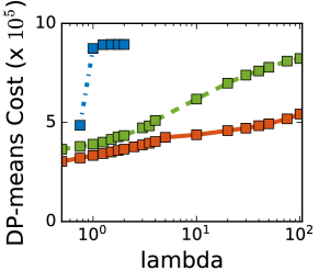
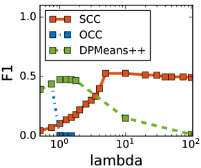
Figure 8: DP-Means and F1 accuracy for ILSVRC (Lg.) dataset

Appendix B Experiments

ILSVRC (Lg.) DP-Means. We replace the SerialDPMeans baseline with its parallel/distributed variant OCC [49]. OCC can only be run with $\lambda<4.0$ (max normalized $\ell_{2}^{2}$ distance). We find that it takes longer than 10 hours to run more than 2 iterations of OCC, for lambda values less than 0.75. After these iterations, we observe that the lambda value of 0.75 gives a reasonable F1 score for OCC. We observe that SCC achieves higher F1 scores when the value of $\lambda$ is larger, as having too small a $\lambda$ value creates too many clusters. We observe that SCC produces lower costs than DPMeans$++$ and achieves a higher F1 value for particular values of $\lambda$.

LowrankALBCD [57] uses values of lambda at the scale of $\lambda=0.01\cdot N$ and normalized $\ell_{2}^{2}$. Any value of $\lambda$ greater than the maximum pairwise distance (4) will result in SerialDPMeans and OCC necessarily giving solutions of every data point in the same cluster. We evaluated LowrankALBCD on CovType, ALOI, Speaker, and ILSVRC (Small). We use the code provided by the authors of LowrankALBCD to solutions with small values of $\lambda$ in the range 0 to 4, for large numbers of iterations we found the code either required more than 100GB of RAM or took longer than 10 hours. Instead, we compare our method and LowrankALBCD for larger values of lambda, specifically the authors suggestion of $0.01N$. We observe that on SCC and LowrankALBCD perform similarly on several of the datasets and LowrankALBCD performs better on CovType. However, we notice that for all datasets except CovType, these values of $\lambda$ produce unreasonably few clusters.

Running Times. We report running times in Table 5. The time required by SCC and Affinity is dominated by the construction of the sparse nearest neighbor graph. We use the publicly available implementations of HDBSCAN and Grinch.

	ALOI	ILSVRC (Sm.)	ILSVRC (Lg.)
HDBSCAN	1635	7902.90	DNF
Grinch	385.113	836.748	DNF
Affinity	29.01 + 0.834	261.831 + 0.298	849.846 + 9.886
SCC	29.01 + 2.79	261.831 + 4.29	849.846 + 65.621

Table 5: Running Time (seconds) of Top Performing Methods. Each run on machine using 24 2.40GHz CPUs. Grinch and HDBSCAN did not finish on largest dataset in 10 hours. Affinity and SCC report Sparse Graph Construction Time + Algorithm Execution Time for given graph. DNF = Did not finish in 10hours.

Robust Hierarchical Clustering (RHC) [5] RHC has stronger theoretical guarantees than SCC. RHC achieves these stronger theoretical guarantees by using a complex linkage function, requiring more time per linkage function execution. In Table 6, we compare the best dendrogram purity achieved by SCC and RHC on the Iris and Wine datasets using a grid search over each method’s hyperparameters ($\alpha+\nu$ for RHC, number of nearest neighbors and rounds for SCC). We use the publicly available MATLAB implementation of RHC. We find on these small datasets that SCC achieves competitive dendrogram purities despite using a simpler linkage function.

	RHC	SCC
Iris	0.955	0.926
Wine	0.944	0.975

Table 6: Comparison to RHC We report the best dendrogram purity achieved across various hyperparameter settings of each method.

References

- Andrews et al. [2014] N. Andrews, J. Eisner, and M. Dredze. Robust entity clustering via phylogenetic inference. ACL, 2014.
- Arthur and Vassilvitskii [2007] D. Arthur and S. Vassilvitskii. k-means++: The advantages of careful seeding. SODA, 2007.
- Bachem et al. [2015] O. Bachem, M. Lucic, and A. Krause. Coresets for nonparametric estimation-the case of dp-means. ICML, 2015.
- Balcan et al. [2008] M. Balcan, A. Blum, and S. Vempala. A discriminative framework for clustering via similarity functions. STOC, 2008.
- Balcan et al. [2014] M. Balcan, Y. Liang, and P. Gupta. Robust hierarchical clustering. JMLR, 2014.
- Bateni et al. [2017] M. Bateni, S. Behnezhad, M. Derakhshan, M. Hajiaghayi, R. Kiveris, S. Lattanzi, and V. Mirrokni. Affinity clustering: Hierarchical clustering at scale. NeurIPS, 2017.
- Benevenuto et al. [2012] F. Benevenuto, T. Rodrigues, M. Cha, and V. Almeida. Characterizing user navigation and interactions in online social networks. Inf. Sci., 2012.
- Beygelzimer et al. [2006] A. Beygelzimer, S. Kakade, and J. Langford. Cover trees for nearest neighbor. ICML, 2006.
- Blundell et al. [2010] C. Blundell, Y. W. Teh, and K. A. Heller. Bayesian rose trees. UAI, 2010.
- Borůvka [1926] O. Borůvka. O jistém problému minimálním. 1926.
- Broderick et al. [2013] T. Broderick, B. Kulis, and M. Jordan. Mad-bayes: Map-based asymptotic derivations from bayes. ICML, 2013.
- Campello et al. [2013] R. J. G. B. Campello, D. Moulavi, and J. Sander. Density-based clustering based on hierarchical density estimates. Advances in Knowledge Discovery and Data Mining, 2013.
- Cao et al. [2006] F. Cao, M. Ester, W. Qian, and A. Zhou. Density-based clustering over an evolving data stream with noise. ICDM, 2006.
- Charikar et al. [2019] M. Charikar, V. Chatziafratis, and R. Niazadeh. Hierarchical clustering better than average-linkage. SODA, 2019.
- Chen et al. [2018] B. Chen, A. Shrivastava, R. C. Steorts, et al. Unique entity estimation with application to the syrian conflict. The Annals of Applied Statistics, 2018.
- Cranmer et al. [2019] K. Cranmer, S. Macaluso, and D. Pappadopulo. Toy generative model for jets. 2019.
- Das et al. [2020] R. Das, A. Godbole, N. Monath, M. Zaheer, and A. McCallum. Probabilistic case-based reasoning for open-world knowledge graph completion. Findings of EMNLP, 2020.
- Dasgupta [2016] S. Dasgupta. A cost function for similarity-based hierarchical clustering. Symposium on Theory of Computing (STOC), 2016.
- [19] L. Ein Dor, Y. Mass, A. Halfon, E. Venezian, I. Shnayderman, R. Aharonov, and N. Slonim. Learning thematic similarity metric from article sections using triplet networks. ACL.
- Eisen et al. [1998] M. B. Eisen, P. T. Spellman, P. O. Brown, and D. Botstein. Cluster analysis and display of genome-wide expression patterns. Proceedings of the National Academy of Sciences, 1998.
- Eriksson et al. [2011] B. Eriksson, G. Dasarathy, A. Singh, and R. Nowak. Active clustering: Robust and efficient hierarchical clustering using adaptively selected similarities. AISTATS, 2011.
- Ester et al. [1996] M. Ester, H.-P. Kriegel, J. Sander, X. Xu, et al. A density-based algorithm for discovering clusters in large spatial databases with noise. KDD, 1996.
- Gavryushkin and Drummond [2016] A. Gavryushkin and A. J. Drummond. The space of ultrametric phylogenetic trees. Journal of theoretical biology, 2016.
- Geusebroek et al. [2005] J. Geusebroek, G. J. Burghouts, and A. W. M. Smeulders. The amsterdam library of object images. IJCV, 2005.
- Gilpin et al. [2013] S. Gilpin, S. Nijssen, and I. Davidson. Formalizing hierarchical clustering as integer linear programming. AAAI, 2013.
- Green et al. [2012] S. Green, N. Andrews, M. R. Gormley, M. Dredze, and C. D. Manning. Entity clustering across languages. NAACL-HLT, 2012.
- Greenberg et al [2014] C. S. Greenberg et al. The nist 2014 speaker recognition i-vector machine learning challenge. Odyssey: The Speaker and Language Recognition Workshop, 2014.
- Großwendt et al. [2019] A. Großwendt, H. Röglin, and M. Schmidt. Analysis of ward’s method. SODA, 2019.
- Guo et al. [2020] R. Guo, P. Sun, E. Lindgren, Q. Geng, D. Simcha, F. Chern, , and S. Kumar. Accelerating large-scale inference with anisotropic vector quantization. In ICML, 2020.
- Heller and Ghahramani [2005a] K. Heller and Z. Ghahramani. Randomized algorithms for fast bayesian hierarchical clustering. EU-PASCAL Statistics and Optimization of Clustering Workshop, 2005a.
- Heller and Ghahramani [2005b] K. A. Heller and Z. Ghahramani. Bayesian hierarchical clustering. ICML, 2005b.
- Jiang et al. [2012] K. Jiang, B. Kulis, and M. I. Jordan. Small-variance asymptotics for exponential family dirichlet process mixture models. NeurIPS, 2012.
- Jin et al [2015] C. Jin et al. A scalable hierarchical clustering algorithm using spark. BigDataService, 2015.
- Kenyon-Dean et al. [2018] K. Kenyon-Dean, J. C. K. Cheung, and D. Precup. Resolving event coreference with supervised representation learning and clustering-oriented regularization. *SEM, 2018.
- Kleinberg [2002] J. Kleinberg. An impossibility theorem for clustering. NeurIPS, 2002.
- Kobren et al. [2017] A. Kobren, N. Monath, A. Krishnamurthy, and A. McCallum. A hierarchical algorithm for extreme clustering. KDD, 2017.
- Kobren et al. [2019] A. Kobren, N. Monath, and A. McCallum. Integrating user feedback under identity uncertainty in knowledge base construction. AKBC, 2019.
- Kranen et al. [2011] P. Kranen, I. Assent, C. Baldauf, and T. Seidl. The clustree: indexing micro-clusters for anytime stream mining. KIS, 2011.
- Krishnamurthy et al. [2012] A. Krishnamurthy, S. Balakrishnan, M. Xu, and A. Singh. Efficient active algorithms for hierarchical clustering. ICML, 2012.
- Kulis and Jordan [2012] B. Kulis and M. I. Jordan. Revisiting k-means: New algorithms via bayesian nonparametrics. ICML, 2012.
- Kushagra et al. [2016] S. Kushagra, S. Samadi, and S. Ben-David. Finding meaningful cluster structure amidst background noise. ALT, 2016.
- Lee et al. [2012] H. Lee, M. Recasens, A. Chang, M. Surdeanu, and D. Jurafsky. Joint entity and event coreference resolution across documents. EMNLP-CoNLL, 2012.
- Mahajan et al. [2009] M. Mahajan, P. Nimbhorkar, and K. Varadarajan. The planar k-means problem is np-hard. WALCOM, 2009.
- Manning et al. [2008] C. D. Manning, P. Raghavan, and H. Schütze. Introduction to Information Retrieval. 2008.
- Monath et al. [2019a] N. Monath, A. Kobren, A. Krishnamurthy, M. R. Glass, and A. McCallum. Scalable hierarchical clustering with tree grafting. KDD, 2019a.
- Monath et al. [2019b] N. Monath, M. Zaheer, D. Silva, A. McCallum, and A. Ahmed. Gradient-based hierarchical clustering using continuous representations of trees in hyperbolic space. KDD, 2019b.
- Moseley and Wang [2017] B. Moseley and J. Wang. Approximation bounds for hierarchical clustering: Average linkage, bisecting k-means, and local search. NeurIPS, 2017.
- Olson [1995] C. F. Olson. Parallel algorithms for hierarchical clustering. Parallel computing, 1995.
- Pan et al. [2013] X. Pan, J. E. Gonzalez, S. Jegelka, T. Broderick, and M. I. Jordan. Optimistic concurrency control for distributed unsupervised learning. NeurIPS, 2013.
- Russakovsky et al [2015] O. Russakovsky et al. Imagenet large scale visual recognition challenge. IJCV, 2015.
- Santos et al. [2019] J. Santos, T. Syed, M. C. Naldi, R. J. Campello, and J. Sander. Hierarchical density-based clustering using mapreduce. TBD, 2019.
- Schwartz et al [2020] G. W. Schwartz et al. TooManyCells identifies and visualizes relationships of single-cell clades. Nat. Methods, 2020.
- Vazirani [2013] V. V. Vazirani. Approximation algorithms. 2013.
- Vitale et al. [2019] F. Vitale, A. Rajagopalan, and C. Gentile. Flattening a hierarchical clustering through active learning. NeurIPS, 2019.
- Yadav et al. [2019] N. Yadav, A. Kobren, N. Monath, and A. McCallum. Supervised hierarchical clustering with exponential linkage. ICML, 2019.
- Yaroslavtsev and Vadapalli [2018] G. Yaroslavtsev and A. Vadapalli. Massively parallel algorithms and hardness for single-linkage clustering under distances. ICML, 2018.
- Yen et al. [2016] I. E. Yen, D. Malioutov, and A. Kumar. Scalable exemplar clustering and facility location via augmented block coordinate descent with column generation. AISTATS, 2016.
- Zaheer et al. [2017] M. Zaheer, S. Kottur, A. Ahmed, J. Moura, and A. Smola. Canopy—fast sampling with cover trees. ICML, 2017.
- Zhang et al. [1996] T. Zhang, R. Ramakrishnan, and M. Livny. Birch: an efficient data clustering method for very large databases. SIGMOD, 1996.
- Zhang et al. [2014] Y. Zhang, A. Ahmed, V. Josifovski, and A. Smola. Taxonomy discovery for personalized recommendation. WSDM, 2014.
- Zhang et al. [2018] Y. Zhang, F. Zhang, P. Yao, and J. Tang. Name disambiguation in AMiner: Clustering, maintenance, and human in the loop. KDD, 2018.
- Zhu and Stuetzle [2019] H. Zhu and W. Stuetzle. A simple and efficient method to compute a single linkage dendrogram. arXiv, 2019.