Four-Dimensional Scaling of Dipole Polarizability in Quantum Systems

Abstract

Polarizability is a key response property of physical and chemical systems, which has an impact on intermolecular interactions, spectroscopic observables, and vacuum polarization. The calculation of polarizability for quantum systems involves an infinite sum over all excited (bound and continuum) states, concealing the physical interpretation of polarization mechanisms and complicating the derivation of efficient response models. Approximate expressions for the dipole polarizability, $\alpha$, rely on different scaling laws $\alpha\propto$ $R^{3}$, $R^{4}$, or $R^{7}$, for various definitions of the system radius $R$. Here, we consider a range of single-particle quantum systems of varying spatial dimensionality and having qualitatively different spectra, demonstrating that their polarizability follows a universal four-dimensional scaling law $\alpha=C(4\mu q^{2}/\hbar^{2})L^{4}$, where $\mu$ and $q$ are the (effective) particle mass and charge, $C$ is a dimensionless excitation-energy ratio, and the characteristic length $L$ is defined via the $\mathcal{L}^{2}$-norm of the position operator. This unified formula is also applicable to many-particle systems, as shown by accurately predicting the dipole polarizability of 36 atoms, 1641 small organic molecules, and Bloch electrons in periodic systems.

The dipole polarizability determines the strength of the response of a system of charged particles to applied electric fields as well as dispersion/polarization interactions between atoms or molecules Stone-book ; Atkins&Friedman-book ; Hermann2017 , playing an important role in the interpretation of experiments Wang2006 ; Dakovski2007 ; Seufert2001 ; Empedocles1997 ; Kulakci2008 . Efficient models for polarizability are useful to predictively describe various phenomena in physics, chemistry, and biology. Moreover, a detailed understanding of quantum-mechanical (QM) polarization mechanisms could help in developing a microscopic picture of intrinsic vacuum response properties Milonni-book ; Leuchs2013 ; Urban2013 . In general, the dipole polarizability is a second-rank tensor which determines the dipole moment induced by an applied electric field: $\mathbf{d}=\tensor{\alpha}\mathbfcal{E}$. For anisotropic systems, the polarizability tensor can be diagonalized using the principal axes, whereas in the case of isotropic systems it effectively reduces to a scalar: $\alpha_{ii}=\alpha=\frac{1}{3}\,{\rm Tr}\,\tensor{\alpha}$. For a QM system in its ground state, the dipole polarizability can be evaluated via the Rayleigh-Schrödinger perturbation theory Atkins&Friedman-book

$$\tensor{\alpha}=2\textstyle\sum\limits^{\infty}_{n\neq 0}{\langle\varPsi_{0}|\hat{\mathbf{d}}|\varPsi_{n}\rangle\otimes\langle\varPsi_{n}|\hat{\mathbf{d}}|\varPsi_{0}\rangle}/{(E_{n}-E_{0})}\ ,$$ (1)

where $\otimes$ indicates the dyadic vector product and the sum goes over all excited states. This formula describes transient or fluctuating electric dipoles as the matrix elements of the dipole operator $\hat{\mathbf{d}}=\sum_{j}\hat{\mathbf{d}}_{j}=\sum_{j}q_{j}\hat{\mathbf{r}}_{j}$, where $q_{j}$ and $\hat{\mathbf{r}}_{j}$ are the charge and position operator of the $j$th particle, respectively. For an accurate calculation of $\alpha$, all bound and continuum states must be taken into account. Thus, Eq. (1), while being exact, is difficult to evaluate in practice. Therefore, various approximations Unsold1927 ; Vinti1932 ; Kirkwood1932 ; Buckingham1979 ; Montgomery2013 have been developed for a more efficient evaluation of Eq. (1). Besides their computational advantage, approximate models often provide a deeper insight into the polarizability and its relation to other physical observables.

According to Eq. (1), the polarizability should be related to a certain characteristic length for a given QM system. This has led to a proposition of a number of scaling laws with respect to different effective system sizes:

$$\alpha\propto R_{\rm cl}^{3}\ ,\ \ \alpha\propto R_{\rm conf}^{4}\ ,\ \ \alpha\propto R_{\rm vdW}^{7}\ .$$ (2)

The first relation stems from the classical formula, $\alpha=(4\pi\epsilon_{0})R_{\rm cl}^{3}$, where $\epsilon_{0}$ is the vacuum permittivity and $R_{\rm cl}$ is the radius of a conducting spherical shell Hirschfelder-book or a hard sphere with uniform electron density and a positive point charge at its center Griffiths-book . This formula delivers the most commonly accepted scaling law, which is used in practice to describe the polarizability of atoms in molecules and materials Johnson2005 ; Mayer2007 ; Tkatchenko2009 ; DeKock2012 ; DelloStritto2019 . The second relation in Eq. (2) holds for confined quantum systems of length $R_{\rm conf}$, as was derived by Fowler Fowler1984 . This relation was observed for semiconductor nanocrystals by using terahertz time-domain spectroscopy Wang2006 ; Dakovski2007 . The third scaling law, $\alpha\propto R_{\rm vdW}^{7}\,$, connecting the atomic polarizability and van der Waals (vdW) radius, was found Fedorov2018 ; Tkatchenko2020 by studying the balance between exchange and correlation forces for two interacting quantum Drude oscillators (QDO) Wang2001 ; Sommerfeld2005 ; Jones2013 . The approach of Ref. Fedorov2018 has been subsequently employed to improve effective models for vdW interactions Silvestrelli2019 ; Rudden2019 . All the three distinct scaling laws can be represented as

$$\alpha=(4\pi\epsilon_{0})R_{p}^{3}\,(R_{p}/R_{p}^{r})^{p}\ ,$$ (3)

where $(R_{p}/R_{p}^{r})^{p}$ is a correction to the classical formula. The renormalization length $R_{p}^{r}$ depends on the choice of the effective system size $R_{p}\in\{R_{\rm cl},R_{\rm conf},R_{\rm vdW}\}$, that corresponds to $p=\{0,1,4\}$. Whereas $R_{1}^{r}$ depends on the system parameters Fowler1984 , $R_{4}^{r}$ was found Fedorov2018 ; Tkatchenko2020 to be the same for all atoms. However, the vdW radius is an interacting radius rather than an effective system size and its accurate evaluation independent from the polarizability is difficult Fedorov2018 . Therefore, it is desirable to establish a general relation of $\alpha$ to a concrete effective size of any given QM system, such as the scaling law for confined systems with a defined confinement radius Fowler1984 . Since Eq. (3) gives the right units of $\alpha$ for any value of $p$, the form of such a general relation is not obvious a priori.

In this Letter, we show that for distinct QM systems the principal-axis components of the polarizability tensor in Eq. (1) are given by a unified expression

$$\alpha_{ii}=C_{i}({4\mu q^{2}}/{\hbar^{2}})L_{i}^{4}\ ,$$ (4)

where the constant $C_{i}$ depends on properties of the quantum particle with mass $\mu$ and charge $q$. The characteristic length $L_{i}$ measures the spatial spread of the ground-state wave function $\Psi_{0}$ with respect to its center of mass $\mathbf{R}=(R_{1},R_{2},...,R_{N})=\langle\Psi_{0}|\hat{\mathbf{r}}|\Psi_{0}\rangle$, which corresponds to the nuclear position in case of atoms. The Euclidean $\mathcal{L}^{2}$-norm of the position vector, $(\mathbf{r}-\mathbf{R})$, is defined for a QM system described by its ground-state wavefunction as

$$L_{i}=\sqrt{\textstyle\int{\,(r_{i}-R_{i})^{2}\,|\Psi_{0}(\mathbf{r})|^{2}}\,\rm d\mathbf{r}^{\emph{N}}}\ ,$$ (5)

where $N$ is the system spatial dimensionality (D). Equation (4), connecting $\alpha_{ii}$ with the characteristic length $L_{i}$ along the $i$th principal axis, makes our approach applicable to QM systems of any dimensionality. Moreover, for atom-like systems with a well-defined positively charged center of mass, the dimensionless constant $C_{i}$ turns out to be close to unity. Equation (4) scales as the relation obtained by Fowler Fowler1984 for confined systems via either an exact derivation of the polarizability or its Unsöld Unsold1927 and Kirkwood Kirkwood1932 estimates. However, the size of such confined systems was imposed as a classical parameter which cannot be defined for QM systems in free space. As we show below, with our choice of the characteristic length – a QM generalization of the conventional Euclidean $\mathcal{L}^{2}$-norm – one can properly describe the polarizability of any atom-like QM system.

To demonstrate the general validity of Eq. (4), we start with the approach of Vinti Vinti1932 , which bridges the Unsöld and Kirkwood approximations, and employ the Integral Mean Value Theorem (IMVT) IMVT1 for the polarizability

$$\alpha_{ii}=({2q^{2}}/{\Delta E_{i}})\textstyle\sum\limits_{n>0}^{\infty}\left\langle\varPsi_{0}\left|\hat{r}_{i}\right|\varPsi_{n}\right\rangle\left\langle\varPsi_{n}\left|\hat{r}_{i}\right|\varPsi_{0}\right\rangle\ ,$$ (6)

by introducing $\Delta E_{i}$ as an effective excitation energy. Based on the IMVT, $\Delta E_{i}$ can be chosen to give the exact polarizability, which differs from the Unsöld approximation Unsold1927 with $\Delta E=E_{1}-E_{0}$ providing an upper bound estimate for the polarizability $\left(\alpha\leq\alpha^{U}\right)$, as was proven variationally by Fowler Fowler1984 . The IMVT allows us to connect the polarizability to the variance of the position operator, $\left(\Delta r_{i}\right)^{2}=\left\langle r_{i}^{2}\right\rangle-\left\langle r_{i}\right\rangle^{2}$, where $\left\langle r_{i}^{2}\right\rangle=\left\langle\varPsi_{0}\left|\hat{r}_{i}^{2}\right|\varPsi_{0}\right\rangle$ and $\left\langle r_{i}\right\rangle=\left\langle\varPsi_{0}\left|\hat{r}_{i}\right|\varPsi_{0}\right\rangle$. Indeed, by using the closure relation  $\sum_{n>0}^{\infty}\left|\varPsi_{n}\right\rangle\left\langle\varPsi_{n}\right|=\mathbb{1}-\left|\varPsi_{0}\right\rangle\left\langle\varPsi_{0}\right|\,$, Eq. (6) reduces to

$$\alpha_{ii}=({2q^{2}}/{\Delta E_{i}})\left(\Delta r_{i}\right)^{2}\ .$$ (7)

Employing now the IMVT IMVT1 for the Thomas-Reiche-Kuhn (TRK) sum-rule Wang1999

$$({2\mu}/\hbar^{2})\textstyle\sum\limits_{n>0}^{\infty}\left(E_{n}-E_{0}\right)\left\langle\varPsi_{0}\left|\hat{r}_{i}\right|\varPsi_{n}\right\rangle^{2}=1\ ,$$ (8)

we obtain another effective excitation energy as $(\Delta\widetilde{E}_{i})^{-1}=({2\mu}/{\hbar^{2}})\left(\Delta r_{i}\right)^{2}$ which fulfills the exact TRK sum-rule. Generally, $\Delta\widetilde{E}_{i}$ is not equal to $\Delta E_{i}$ in Eq. (6) but there is a constant $C_{i}$ such that $\Delta\widetilde{E}_{i}=C_{i}\,\Delta E_{i}$. Inserting $(\Delta E_{i})^{-1}=C_{i}\,({2\mu}/{\hbar^{2}})\left(\Delta r_{i}\right)^{2}$ into Eq. (7) yields

$$\alpha_{ii}=C_{i}\,({4\mu q^{2}}/{\hbar^{2}})\left(\Delta r_{i}\right)^{4}=C_{i}\,({4\mu q^{2}}/{\hbar^{2}})\,L_{i}^{4}\ ,$$ (9)

where we used the fact that $L_{i}^{2}$ defined via Eq. (5) is identical to the variance, $(\Delta r_{i})^{2}$. With $C_{i}=1$ in Eq. (9), i.e. $\Delta\widetilde{E}=\Delta E$, we reproduce Vinti’s original derivation Vinti1932 of the well-known Kirkwood formula Kirkwood1932 , which yields a lower bound to the exact polarizability $\left(\alpha^{K}\leq\alpha\right)$ Fowler1984 . The general formula, Eqs. (4) and (9), is based on fundamental properties of QM systems caused by quantum fluctuations, which determine and relate $L_{i}$ in Eq. (5) as the ground-state metric of the position operator to $\alpha_{ii}$ as determined by the transient electric dipoles in Eq. (1).

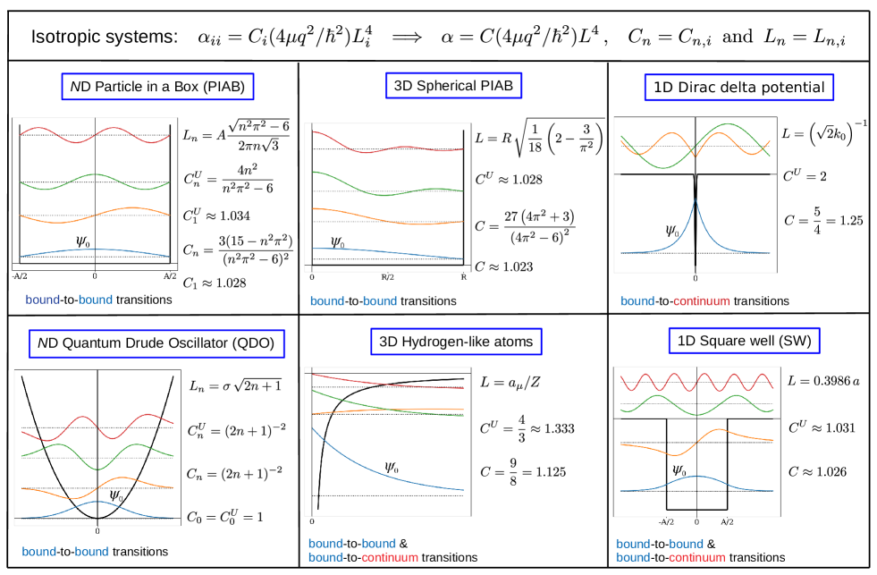
Figure 1: The exact and Unsöld ($U$) polarizability of six different quantum-mechanical models is represented by the general formula of Eq. (4), where the characteristic length $L$ is calculated for each system according to the same unified definition given by Eq. (5). The Cartesian indices ($ii$) are dropped since all the models are isotropic. For the $N$-dimensional ($N$D) PIAB and QDO, $n$ denotes the quantum number of excited states (with $n=1$ and $n=0$, respectively, for the ground state). For the other systems, only the ground state polarizabilty is evaluated. Furthermore, $A$, $k_{0}$, $R$, $r_{0}$ are the parameters of the potentials for the given systems Supplementary . Then, $\sigma^{2}$ is the variance of the harmonic oscillator, $Ze$ is the nuclear charge for the hydrogen-like atoms, and $a_{\mu}=(4\pi\epsilon_{0})\hbar^{2}/\mu e^{2}$. The 1D square well is considered with the depth $V_{0}$ and the width $A$ related as $\displaystyle V_{0}=100\hbar^{2}/2\mu A^{2}$.

To assess the scope of validity of Eq. (4), we analysed several isotropic QM models: (i) particle in a box (PIAB) of an arbitrary dimension; (ii) particle confined in a sphere; (iii) 1D Dirac delta potential; (iv) square well (SW) in 1D; (v) quantum Drude oscillator (QDO) in an arbitrary dimension; (vi) 3D hydrogen-like atoms. These model systems are chosen since they allow one to obtain exact analytical solutions for their spectrum and polarizability containing a wide variety of features representing real molecules and materials. Figure 1 summarizes the obtained polarizabilities for these models, whereas the detailed derivations are given in the Supplemental Material (SM) Supplementary . We show that each system obeys the formula given by Eq. (4) with $L=L_{i}$ defined by Eq. (5) for all models and constant $C=C_{i}$ being close to unity. This is remarkable since the chosen systems possess qualitatively different energy spectra: the PIAB and QDO have bound excited states only, while the 1D Dirac delta potential has solely excitations to the continuum; on the other hand, for the hydrogen-like atoms and SW, both bound and continuum states are present. Moreover, the polarizability of excited states of PIAB and QDO follow the same $L^{4}$ scaling law of Eq. (4), as shown by a straightforward generalization of our approach to an arbitrary QM state Supplementary . Thus, the polarizability of different models, regardless of their spatial dimension, excitation state and spectra, can be expressed by Eq. (4).

The difference between the model systems is reflected in both, the characteristic length and dimensionless constant entering Eq. (4), but only $L$ contains the system parameters, while $C$ is independent of their actual values. As shown by Fig. 1, qualitatively similar systems have practically the same constant: $1.023<C<1.028$, for $N$D PIAB, 3D Spherical PIAB, and 1D SW (with $\displaystyle V_{0}=100\hbar^{2}/2\mu A^{2}$), as the cases of confined particles. For 1D SW, in the limit of vanishing potential depth, only one bound state remains resulting in $C=1.25$ Supplementary , which is similar to 1D delta potential with just one bound state and $C=1.25$. For hydrogen-like atoms and the QDO, we obtain $C=1.125$ and $C=1$, respectively. As mentioned above, the Kirkwood approximation gives $C^{K}=1$ in all cases. Figure 1 also shows $C^{U}$ obtained within the Unsöld approximation, the upper bound of $C$. For the QDO, both approximations deliver the exact result, $C=1$. Thus, for atom-like systems in their ground state, $\Delta C$ in $C=1+\Delta C$ measures the strength of anharmonic contributions from quantum fluctuations versus the dominant harmonic part. The largest anharmonic contribution, $\Delta C=0.25$, is found for 1D delta potential and SW with vanishing potential depth Supplementary . Remarkably, for hydrogen-like atoms, $\Delta C=0.125$ is exactly twice less than $\Delta C=0.25$ obtained for the two systems with just one bound state. For the other three systems with confined particles, $\Delta C$ is vanishingly small, similar to the harmonic potential. For excited states, $C$ can strongly deviate from unity depending on corresponding quantum numbers (see Fig. 1 and the SM Supplementary ), but the $L^{4}$ scaling remains valid. Altogether, this demonstrates that the general form of Eq. (4) is valid for all single-particle systems shown in Fig. 1. Furthermore, in the SM Supplementary we consider the nearly free electron model and show that the same scaling law holds for Bloch electrons.

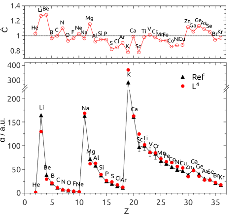
Figure 2: Polarizabilities of multi-electron atoms calculated using ground-state DFT/PBE0 orbitals and the quantum-mechanical ($L^{4}$) scaling law. The lower panel demonstrates $\alpha$ calculated by Eq. (10) with ${\tilde{C}}=C_{k}=1$. The upper panel shows ${\tilde{C}}$ obtained by comparison of Eq. (10) to the reference polarizabilities Atomic_alpha_ref . Further details are given in the SM Supplementary .

In the SM Supplementary , we discuss an extension of Eq. (4) to a general many-particle system. Here, we consider many-electron atoms by applying Eq. (4) to each electron shell. In such a case, the (isotropic) atomic polarizability reads

$$\alpha=\tfrac{4m_{e}e^{2}}{\hbar^{2}}\textstyle\sum\limits_{k}^{\text{occ}}\frac{C_{k}}{\eta_{k}}\frac{L_{k}^{4}}{N_{k}}\approx{\tilde{C}}\left(\frac{4m_{e}e^{2}}{\hbar^{2}}\right)\textstyle\sum\limits_{k}^{\text{occ}}\frac{L_{k}^{4}}{\eta_{k}N_{k}}\ ,$$ (10)

where the sum runs over occupied orbitals with degenerate states treated together Supplementary , $L_{k}$ is obtained by Eq. (5) for the $k$th orbital and $N_{k}$ is its occupation number stemming from the many-electron version of the TRK sum-rule. Then, $\eta_{k}$ are orbital-dependent factors required for all atoms starting from Li ($\eta_{k}^{{}_{\rm He}}=1$), empirically found by us to be $\eta_{k}=n_{k}^{{}_{\ell}}N_{k}^{{}_{[1+(-1)^{\ell}]/2}}$, where $\ell$ and $n_{k}$ are, respectively, the orbital and principal quantum numbers of the $k$th orbital Supplementary . Based on our results for single-particle models, we assume all $C_{k}$ to be close to each other, which allows us to make the approximation given by the r.h.s. of Eq. (10). As shown in Fig. 2, the coarse-grained constant ${\tilde{C}}$ is close to unity for different atoms. Hence, the response of each electronic orbital in an atom is well approximated by Eq. (10) with $C_{k}=1$. This means that we approximate each orbital in a many-electron atom by an effective quantum harmonic oscillator, where the screening of nuclear charge caused by the presence of occupied orbitals is taken into account via $\eta_{k}$. In particular, ${\tilde{C}}\approx 1$ for noble gases from He to Kr, for which the QDO model is known to work well Jones2013 ; Fedorov2018 . Unlike single-particle systems, for many-electron atoms ${\tilde{C}}$ can be lower than unity, and we attribute this to correlation effects between electronic shells that should be explicitly included for a more accurate treatment. Equation (10) significantly improves over the many-electron version of the Kirkwood approximation derived by Buckingham Buckingham1937 , which corresponds to setting $C_{k}/\eta_{k}=1$ in Eq. (10) and treating all orbitals equally. Such approximation yields an overestimation up to a factor of 4 for the polarizabilities shown in Fig. 2 Supplementary .

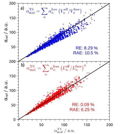
Figure 3: Comparing two implementations of the Tkatchenko-Scheffler (TS) method Tkatchenko2009 : (a) the conventional TS method based on Eq. (11) and (b) the modified TS method based on Eq. (12). The corresponding molecular polarizabilities $\alpha_{\rm mol}^{\rm{TS}}$ are shown versus the reference values $\alpha_{\rm{ref}}$ calculated by using density-functional theory (DFT) with PBE0 functional Comment_2 .

Let us now apply Eq. (4) to compute polarizabilities of 1641 small organic molecules from the TABS dataset Blair2014_1 by employing the Tkatchenko-Scheffler (TS) method Tkatchenko2009 , which is widely used for vdW-inclusive density-functional calculations. Due to the commonly assumed direct proportionality between the atomic volume and polarizability, within the TS method molecular polarizabilities are approximated by a sum of effective atomic polarizabilities expressed in terms of the polarizabilities of free atoms as

$$\alpha_{\rm mol}^{\rm TS}=\textstyle\sum\limits_{n}\alpha_{n}^{\rm eff}=\sum\limits_{n}\alpha_{n}^{\rm free}\left({V_{n}^{\rm{eff}}}/V_{n}^{\rm{free}}\right)\ ,$$ (11)

where the sum runs over all atoms in the molecule. The weights $\left({V_{n}^{\rm{eff}}}/V_{n}^{\rm{free}}\right)$ measuring the volume ratio for atom in a molecule to the free atom in vacuum are obtained by the Hirshfeld partitioning of the electron density Hirshfeld1977 . Based on the relation of Eq. (4), we modify Eq. (11) to

$$\alpha_{\rm mol}^{\rm TS}=\textstyle\sum\limits_{n}\alpha_{n}^{\rm eff}=\sum\limits_{n}\alpha_{n}^{\rm free}({L_{n}^{\rm{eff}}}/L_{n}^{\rm{free}})^{4}\ ,$$ (12)

which allows us to keep the simplicity of the TS method but make it consistent with the $L^{4}$ scaling law. Figure 3 shows that by using Eq. (12) instead of Eq. (11) the average signed relative error $\langle{\rm RE}\rangle$ drops from 8.29% to 0.09%. The practically vanishing systematic deviation and the decrease of the average absolute relative error $\langle{\rm RAE}\rangle$ from 10.5% to 6.25% confirm the applicability of the employed scaling law. The remaining deviations from reference DFT results can be attributed to the anisotropy of molecular polarizability, which necessitates an explicit coupling between atomic polarizabilities Tkatchenko2012 . A detailed analysis performed in the SM Supplementary shows that among other possible scaling laws Eq. (12) provides the best accuracy for the TS method, which serves as an additional argument Comment_3 for the general validity of Eq. (4).

In summary, we have established a general formula for the dipole polarizability, $\alpha=C(4\mu q^{2}/\hbar^{2})L^{4}$, valid for QM systems of varying spatial dimension, symmetry, excitation state, and number of particles. The universality of the $L^{4}$ scaling for $\alpha$ is connected to the unified QM metric $L$ measuring fluctuations of the particle position in terms of the system parameters. By contrast, the dimensionless coefficient $C$ reflects just the qualitative properties of the eigenvalue spectrum of each system. The geometric scaling of the polarizability for a system in its ground state is solely determined by the ground-state wavefunction, whereas the effect of excited states is encoded in $C$ only. Another interesting finding is that the polarizability expression in Eq. (4) is directly proportional to the particle mass, which is opposite to the classical picture where the polarizability vanishes for infinite particle mass. Our formula can be used to improve DFT-based methods for vdW interactions Hermann2017 ; Tkatchenko2009 , parametrize polarizable force fields Wang2001 ; Sommerfeld2005 ; Jones2013 , or efficiently calculate dynamic spectroscopic observables based on the polarizability (i.e., Raman and sum-frequency generation) Wang2006 ; Dakovski2007 ; Seufert2001 ; Empedocles1997 ; Kulakci2008 . These applications rely on efficient and accurate evaluation of polarizability from ground-state electron density.

The authors acknowledge financial support from the Luxembourg National Research Fund: FNR CORE projects “QUANTION(C16/MS/11360857, GrNum:11360857)” and “PINTA(C17/MS/11686718)”, AFR PhD Grant “POMO(AFR PhD/19/MS, GrNum:13590856)”, and “DRIVEN” (PRIDE17/12252781) under the PRIDE program. Furthermore, the financial support from European Research Council, ERC Consolidator Grant “BeStMo(GA n725291)” and INTER-FWO project “MONODISP”, is also gratefully acknowledged.

References

- (1) A. Stone, The Theory of Intermolecular Forces, (Oxford University Press, 2016).
- (2) P. Atkins and R. Friedman, Molecular Quantum Mechanics, (Oxford University Press, 2005).
- (3) J. Hermann, R. A. DiStasio Jr., and A. Tkatchenko, First-Principles Models for van der Waals Interactions in Molecules and Materials: Concepts, Theory, and Applications, Chem. Rev. 117, 4714 (2017)
- (4) F. Wang, J. Shan, M.A. Islam, I.P. Herman, M. Bonn, T.F. Heinz, Exciton polarizability in semiconductor nanocrystals, Nat. Mater. 5, 861 (2006).
- (5) G. L. Dakovski, S. Lan, C. Xia, J. Shan, Terahertz Electric Polarizability of Excitons in PbSe and CdSe Quantum Dots, J. Phys. Chem. C 111, 5904 (2007).
- (6) J. Seufert, M. Obert, M. Scheibner, N.A. Gippius, G. Bacher, A. Forchel, T. Passow, K. Leonardi, D. Hommel, Stark effect and polarizability in a single CdSe/ZnSe quantum dot, App. Phys. Lett. 79, 1033 (2001).
- (7) S.A. Empedocles, M.G. Bawendi, Quantum-Confined Stark Effect in Single CdSe Nanocrystallite Quantum Dots, Science 278, 2114 (1997).
- (8) M. Kulakci, U. Serincan, R. Turan, T.G. Finstad, The quantum confined Stark effect in silicon nanocrystals, Nanotechnology 19, 455403 (2008).
- (9) P.W. Milonni, The Quantum Vacuum: An Introduction to Quantum Electrodynamics, (Academic Press, 1993).
- (10) G. Leuchs and L. L. Sánchez-Soto, A sum rule for charged elementary particles, Eur. Phys. J. D 67, 57 (2013).
- (11) M. Urban, F. Couchot, X. Sarazin, and A. Djannati-Atai, The quantum vacuum as the origin of the speed of light, Eur. Phys. J. D 67, 58 (2013).
- (12) A. Unsöld, Quantentheorie des Wasserstoffmolekülions und der Born-Landéschen Abstoßungskräfte, Z. Physik 43, 563 (1927).
- (13) J. P. Vinti, A Relation between the Electric and Diamagnetic Susceptibilities of Monatomic Gases, Phys. Rev. 41, 813 (1932).
- (14) J. G. Kirkwood, Polarisierbarkeiten, Suszeptibilitäten und van der Waalssche Kräfte der Atome mit mehreren Elektronen, Phys. Z. 33, 57 (1932).
- (15) A.D. Buckingham, Polarizability and hyperpolarizability, Phil. Trans. R. Soc. Lond. A 293, 239 (1979).
- (16) H. E. Montgomery Jr. and V. I. Pupyshev, On the lower bounds of polarisability, Eur. Phys. J. H. 38, 519 (2013).
- (17) J. O. Hirschfelder, C. F. Curtiss, and R. B. Bird, Molecular Theory of Gases and Liquids, (Wiley-Interscience, New York, 1964).
- (18) D. J. Griffiths, Introduction to Electrodynamics, (Cambridge University Press, 2017).
- (19) E. R. Johnson and A. D. Becke, A post-Hartree–Fock model of intermolecular interactions, J. Chem. Phys. 123, 024101 (2005).
- (20) A. Mayer, Formulation in terms of normalized propagators of a charge-dipole model enabling the calculation of the polarization properties of fullerenes and carbon nanotubes, Phys. Rev. B 75, 045407 (2007).
- (21) A. Tkatchenko and M. Scheffler, Accurate Molecular Van Der Waals Interactions from Ground-State Electron Density and Free-Atom Reference Data, Phys. Rev. Lett. 102, 073005 (2009).
- (22) R. L. DeKock, J. R. Strikwerda, and E. X. Yu, Atomic size, ionization energy, polarizability, asymptotic behavior, and the Slater-Zener model, Chem. Phys. Lett. 547, 120 (2012).
- (23) M. DelloStritto, M.L. Klein, and E. Borguet, Bond-Dependent Thole Model for Polarizability and Spectroscopy, J. Phys. Chem. A 123, 5378 (2019).
- (24) P. W. Fowler, Energy, polarizability and size of confined one-electron systems, Mol. Phys. 53, 865 (1984).
- (25) D. V. Fedorov, M. Sadhukhan, M. Stöhr, and A. Tkatchenko, Quantum-Mechanical Relation between Atomic Dipole Polarizability and the van der Waals Radius, Phys. Rev. Lett. 121, 183401 (2018).
- (26) A. Tkatchenko, D. V. Fedorov and M. Gori, Fine-Structure Constant Connects Electronic Polarizability and Geometric van-der-Waals Radius of Atoms , J. Phys. Chem. Lett. 12, 9488 (2021).
- (27) F. Wang and K. D. Jordan, A Drude-model approach to dispersion interactions in dipole-bound anions, J. Chem. Phys. 114, 10717 (2001).
- (28) T. Sommerfeld and K. D. Jordan, Quantum Drude Oscillator Model for Describing the Interaction of Excess Electrons with Water Clusters: An Application to (H2O), J. Phys. Chem. A 109, 11531 (2005).
- (29) A. P. Jones, J. Crain, V. P. Sokhan, T. W. Whitfield, and G. J. Martyna, Quantum Drude oscillator model of atoms and molecules: Many-body polarization and dispersion interactions for atomistic simulation, Phys. Rev. B 87, 144103 (2013).
- (30) P. L. Silvestrelli and A. Ambrosetti, van der Waals interactions in DFT using Wannier functions without empirical parameters, J. Chem. Phys. 150, 164109 (2019).
- (31) L. S. P. Rudden and M. T. Degiacomi, Protein Docking Using a Single Representation for Protein Surface, Electrostatics, and Local Dynamics, J. Chem. Theory Comput. 15, 5135 (2019).
- (32) The integral mean value theorem IMVT2 : If is a continuous real function on and is Riemann integrable on such that either or , then there exists a real number such that .
- (33) S. Wang, Generalization of the Thomas-Reiche-Kuhn and the Bethe sum rules, Phys. Rev. A 60, 262 (1999).
- (34) See Supplemental Material at http://link.aps.org/supplemental/… , which includes Refs. Flugge1994 ; Brownstein1975 ; Griffiths2018 ; Maize2011 ; Dalgarno1955 ; Kharchenko2015 ; Slater1951 ; Jensen2001 ; Ashcroft2005 , for a detailed consideration of model systems as well as many-electron atoms and molecules.
- (35) S. Flügge, Practical Quantum Mechanics, (Springer-Verlag, 1994).
- (36) K. R. Brownstein, Calculation of a bound state wave function using free state wave functions only, Am. J. Phys. 43, 173 (1975).
- (37) D. J. Griffiths, Introduction to quantum mechanics, (Cambridge University Press, 2018).
- (38) M. A. Maize, M. A. Antonacci, and F. Marsiglio, The static electric polarizability of a particle bound by a finite potential well, Am. J. Phys. 79, 222 (2011).
- (39) A. Dalgarno and J. T. Lewis, The exact calculation of long-range forces between atoms by perturbation theory, Proc. R. Soc. A 233, 70 (1955).
- (40) V. F. Kharchenko, Analytical transition-matrix treatment of electric multipole polarizabilities of hydrogen-like atoms, Ann. Phys. 355, 153 (2015).
- (41) J. C. Slater, Quantum Theory of Matter, (McGraw-Hill, 1951).
- (42) F. Jensen, Polarization consistent basis sets: Principles, J. Chem. Phys. 115, 9113 (2001).
- (43) N. W. Ashcroft and N. D. Mermin, Solid State Physics, (Holt, Rinehart, and Winston, New York, 2005).
- (44) R. A. Buckingham, The Quantum Theory of Atomic Polarization. I. Polarization by a Uniform Field, Proc. R. Soc. Lond. A 160, 94 (1937).
- (45) P. Schwerdtfeger, J. K. Nagle, 2018 Table of static dipole polarizabilities of the neutral elements in the periodic table, Mol. Phys. 117, 1200 (2019).
- (46) S. A. Blair and A. J. Thakkar, TABS: A database of molecular structures, Comput. Theor. Chem. 1043, 13 (2014).
- (47) The structures of the TABS database were taken from Ref. Blair2014_1 . Reference molecular polarizability calculations were performed by means of the FHI-aims code Blum2009 using density functional perturbation theory with the hybrid PBE0 functional employing tight numerical basis set for all systems. The Hirshfeld volumes Hirshfeld1977 for the same geometries were calculated using the PBE functional.
- (48) F. L. Hirshfeld, Bonded-atom fragments for describing molecular charge densities, Theor. Chem. Acc. 44, 129 (1977).
- (49) A. Tkatchenko, R. A. DiStasio, Jr., R. Car, and M. Scheffler, Accurate and Efficient Method for Many-Body van der Waals Interactions, Phys. Rev. Lett. 108, 236402 (2012).
- (50) Authors of Ref. Blair2014_2 also found that the molecular dipole polarizabilities from the TABS database Blair2014_1 seem to scale as . However, their empirical finding was reported without giving any fundamental reason for this non-linear relation. In addition, for atoms, the relation was discussed in Refs. Gobre2016 and Kleshchonok2018 as derived within the QDO model Wang2001 ; Sommerfeld2005 ; Jones2013 , where is the variance of the quantum Drude/harmonic oscillator Supplementary .
- (51) P. K. Sahoo and T. Riedel, Mean Value Theorems and Functional Equations, (World Scientific Publishing Company, 1998).
- (52) V. Blum, R. Gehrke, F. Hanke, P. Havu, V. Havu, X. Ren, K. Reuter, and M. Scheffler, Ab initio molecular simulations with numeric atom-centered orbitals, Comput. Phys. Commun. 180, 2175 (2009).
- (53) S. A. Blair and A. J. Thakkar, Relating polarizability to volume, ionization energy, electronegativity, hardness, moments of momentum, and other molecular properties, J. Chem. Phys. 141, 074306 (2014).
- (54) V. V. Gobre, Efficient modelling of linear electronic polarization in materials using atomic response functions, PhD thesis, Fritz Haber Institute Berlin (2016).
- (55) A. Kleshchonok and A. Tkatchenko, Tailoring van der Waals dispersion interactions with external electric charges, Nat. Commun. 9, 3017 (2018).