Should Graph Convolution Trust Neighbors? A Simple Causal Inference Method

Abstract.

Graph Convolutional Network (GCN) is an emerging technique for information retrieval (IR) applications. While GCN assumes the homophily property of a graph, real-world graphs are never perfect: the local structure of a node may contain discrepancy, e.g., the labels of a node’s neighbors could vary. This pushes us to consider the discrepancy of local structure in GCN modeling. Existing work approaches this issue by introducing an additional module such as graph attention, which is expected to learn the contribution of each neighbor. However, such module may not work reliably as expected, especially when there lacks supervision signal, e.g., when the labeled data is small. Moreover, existing methods focus on modeling the nodes in the training data, and never consider the local structure discrepancy of testing nodes.

This work focuses on the local structure discrepancy issue for testing nodes, which has received little scrutiny. From a novel perspective of causality, we investigate whether a GCN should trust the local structure of a testing node when predicting its label. To this end, we analyze the working mechanism of GCN with causal graph, estimating the causal effect of a node’s local structure for the prediction. The idea is simple yet effective: given a trained GCN model, we first intervene the prediction by blocking the graph structure; we then compare the original prediction with the intervened prediction to assess the causal effect of the local structure on the prediction. Through this way, we can eliminate the impact of local structure discrepancy and make more accurate prediction. Extensive experiments on seven node classification datasets show that our method effectively enhances the inference stage of GCN.

1. Introduction

GCN is being increasingly used in IR applications, ranging from search engines (Mao et al., 2020; Yang, 2020), recommender systems (Wang et al., 2019a; Chen et al., 2019a; He et al., 2020; Chen et al., 2020a) to question-answering systems (Zhang et al., 2020b; Hu et al., 2020c). Its main idea is to augment a node’s representation by aggregating the representations of its neighbors. In practice, GCN could face the local structure discrepancy issue (Chen et al., 2020c) since real-world graphs usually exhibit locally varying structure. That is, nodes can exhibit inconsistent distributions of local structure properties such as homophily and degree. Figure 1 shows an example in a document citation graph (Hu et al., 2020a), where the local structure centered at $node1$ and $node2$ has different properties regarding cross-category edges. Undoubtedly, applying the same aggregation over $node1$ and $node2$ will lead to inferior node representations. Therefore, it is essential for GCN to account for the local structure discrepancy issue.

Existing work considers this issue by equipping GCN with an adaptive locality module (Xu et al., 2018; Veličković et al., 2018), which learns to adjust the contribution of neighbors. Most of the efforts focus on the attention mechanism, such as neighbor attention (Veličković et al., 2018) and hop attention (Liu et al., 2020). Ideally, the attention weight could downweigh the neighbors that causes discrepancy, e.g., the neighbors of different categories with the target node. However, graph attention is not easy to be trained well in practice, especially for hard semi-supervised learning setting that has very limited labeled data (Knyazev et al., 2019). Moreover, existing methods mainly consider the nodes in the training data, ignoring the local structure discrepancy on the testing nodes, which however are the decisive factor for model generalization. It is thus insufficient to resolve the discrepancy issue by adjusting the architecture of GCN.

In this work, we argue that it is essential to empower the inference stage of a trained GCN with the ability of handling the local structure discrepancy issue. In real-world applications, the graph structure typically evolves along time, resulting in structure discrepancy between the training data and testing data. Moreover, the testing node can be newly coming (e.g., a new user), which may exhibit properties different from the training nodes (Tang et al., 2020b). However, the one-pass inference procedure of existing GCNs indiscriminately uses the learned model parameters to make prediction for all testing nodes, lacking the capability of handling the structure discrepancy. This work aims to bridge the gap by upgrading the GCN inference to be node-specific according to the extent of structure discrepancy.

To achieve the target, the key lies in analyzing the prediction generation process of GCN on each node and estimating to what extent accounting for node’s neighbors affects its prediction, i.e., the causal effect of the local structure on GCN prediction. According to the evidence that model output can reflect feature discrepancy (Saito et al., 2018), we have a key assumption that the GCN output provides evidence on the properties of the local structure centered at a testing node. For instance, if the local structure exhibits properties distinct from the seen ones, the model will be uncertain about its prediction when the neighbors are taken into account. Accordingly, we should downweigh the contribution of neighbors to reduce the impact of the discrepancy on the prediction. Inherently, both a node’s features and neighbors are the causes of the prediction for the node. By distinguishing the two causal effects, we can assess revise the model prediction in a node-specific manner.

To this end, we resort to the language of causal graph (Pearl, 2009) to describe the causal relations in GCN prediction. We propose a Causal GCN Inference (CGI) model, which adjusts the prediction of a trained GCN according to the causal effect of the local structure. In particular, CGI first calls for causal intervention that blocks the graph structure and forces the GCN to user a node’s own features to make prediction. CGI then makes choice between the intervened prediction and the original prediction, according to the causal effect of the local structure, prediction confidence, and other factors that characterize the prediction. Intuitively, CGI is expected to choose the intervened prediction (i.e., trusting self) when facing a testing node with local structure discrepancy. To learn a good choice-making strategy, we devise it as a separate classifier, which is learned based on the trained GCN. We demonstrate CGI on APPNP (Klicpera et al., 2019), one of the state-of-the-art GCN models for semi-supervised node classification. Extensive experiments on seven datasets validate the effectiveness of our approach. The codes are released at: https://github.com/fulifeng/CGI.

The main contributions of this work are summarized as follows:

• We achieve adaptive locality during GCN inference and propose an CGI model that is model-agnostic.

• We formulate the causal graph of GCN working mechanism, and the estimation of causal intervention and causal uncertainty based on the causal graph.

• We conduct experiments on seven node classification datasets to demonstrate the rationality of the proposed methods.

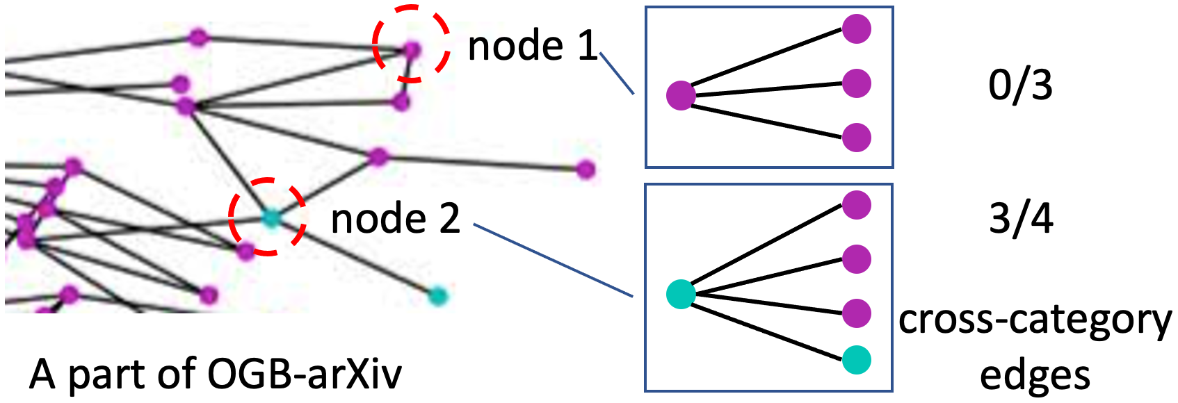
Figure 1. Illustration of local structure discrepancy in OGB-arXiv (Hu et al., 2020a), a citation graph of papers. Nodes in different colors belong to different categories.

2. Preliminaries

Node classification.

We represent a graph with $N$ nodes as $G=(\bm{A},\bm{X})$, i.e., an adjacency matrix $\bm{A}\in\mathbb{R}^{N\times N}$ associated with a feature matrix $\bm{X}=[\bm{x}_{1},\bm{x}_{2},\cdots,\bm{x}_{N}]^{T}\in\mathbb{R}^{N\times D}$. $\bm{A}$ describes the connections between nodes where $A_{ij}=1$ means there is an edge between node $i$ and $j$, otherwise $A_{ij}=0$. $D$ is the dimension of the input node features.Node classification is one of the most popular analytic tasks on graph data. In the general problem setting, the label of $M$ nodes are given $\bm{Y}=[\bm{y}_{1},\bm{y}_{2},\cdots,\bm{y}_{N}]^{T}\in\mathbb{R}^{N\times L}$, where $L$ is the number of node categories and $\bm{y}_{1}$ is a one-hot vector. The target is to learn a classifier from the labeled nodes, formally,

(1) $$f(\bm{x},\mathcal{N}(\bm{x})|\bm{\theta}),~{}\mathcal{N}(\bm{x})=\{\bm{x}_{n}|\bm{A}_{in}=1\},$$

where $\bm{\theta}$ denotes the parameter of the classifier and $\mathcal{N}(\bm{x})$ denotes the neighbor nodes of the target node $\bm{x}$. Without loss of generality, we index the labeled nodes and testing nodes in the range of $[1,M]$ and $(T,N]$, respectively. There are four popular settings with minor differences regarding the observability of testing nodes during model training and the amount of labeled nodes. Specifically,

• Inductive Full-supervised Learning: In this setting, testing nodes are not included in the graph used for model training and all training nodes are labeled. That is, $M=T$ and learning the classifier with $f(\bm{X}_{tr}|\bm{A}_{tr},\bm{\theta})$ where $\bm{X}_{tr}\in\mathbb{R}^{M\times D}$ and $\bm{A}_{tr}$ denotes the features and the subgraph of the training nodes.

• Inductive Semi-supervised Learning (Hamilton et al., 2017): In many real-world applications such as text classification (Linmei et al., 2019), it is unaffordable to label all the observed nodes, i.e., only a small portion of the training nodes are labeled (in fact, $M\ll T$).

• Transductive Full-supervised Learning (Hu et al., 2020a): In some cases, the graph is relatively stable, i.e., no new node occurs, where the whole node graph $\bm{X}$ and $\bm{A}$ are utilized for model training.

• Transductive Semi-supervised Learning (Kipf and Welling, 2017): In this setting, the whole graph is available for model training while only a small portion of the training nodes are labeled.

It should be noted that we do not restrict our problem setting to be a specific one like most previous work on GCN, since we focus on the general inference model.

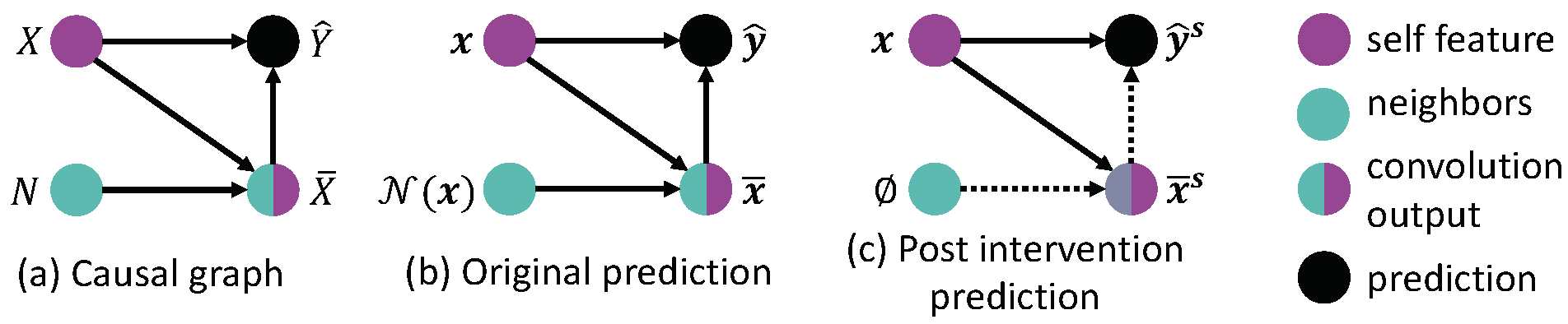
Figure 2. Cause-effect view of GCN. (a) Causal graph of GCN inference process; (b) making original prediction; (c) causal intervention $do(N=\emptyset)$ where dashed arrow means the effect from the predecessor is blocked.

Graph Convolutional Network.

Taking the graph as input, GCN learns node representations to encode the graph structure and node features (the last layer makes predictions) (Kipf and Welling, 2017). The key operation of GCN is neighbor aggregation, which can be abstracted as:

(2) $$\bar{\bm{x}}=AGG(\bm{x},\{\bm{x}_{n}|\bm{x}_{n}\in\mathcal{N}(\bm{x})\}),$$

where $AGG$ denotes the node aggregation operation such as a weighted summation (Kipf and Welling, 2017). $\bm{x}$ and $\bar{\bm{x}}\in\mathbb{R}^{D}$ are the origin representation of the target node (node features or representation at the previous layer) and the one after aggregating neighbor node features. Note that standard GCN layer typically consists a feature transformation, which is omitted for briefness.

Adaptive locality.

In most GCN, the target node is equally treated as the neighbor nodes, i.e., no additional operation except adding the edge for self-connection. Aiming to distinguish the contribution from target node and neighbor nodes, a self-weight $\alpha$ is utilized, i.e., $\mathcal{N}(\alpha*\bm{x},\{(1-\alpha)*\bm{x}_{n}|n\in neighbor(\bm{x})\})$. More specifically, neighbor attention (Veličković et al., 2018) is introduced to learn node specific weights, i.e., $\mathcal{N}(\alpha\bm{x},\{\alpha_{n}*\bm{x}_{n}|n\in neighbor(\bm{x})\})$. The weights $\alpha$ and $\alpha_{n}$ are calculated by an attention model such as multi-head attention (Vaswani et al., 2017) with the node representations $\bm{x}$ and $\bm{x}_{n}$ as inputs. Lastly, hop attention (Liu et al., 2020) is devised to adaptively aggregate the target node representations at different GCN layers $\bm{x}^{0},\cdots,\bar{\bm{x}}^{k},\cdots,\bar{\bm{x}}^{K}$ into a final representation. $\bar{\bm{x}}^{k}$ is the convolution output at the $k$-th layer which encodes the $k$-hop neighbors of the target node. For a target node that is expected to trust self more, the hop attention is expected to assign higher weight for $\bm{x}^{0}$. Most of these adaptive locality models are learned during model training except the self-weight $\alpha$ in GCN models like APPNP which is tuned upon the validation set.

Causal effect.

Causal effect is a concept in causal science (Pearl, 2009), which studies the influence among variables. Given two variables $X$ and $Y$, the causal effect of $X=x$ on $Y$ is to what extent changing the value of $X$ to $x$ affects the value of $Y$, which is abstracted as:

(3) $$Y_{x}-Y_{x^{*}},$$

where $Y_{x}$ and $Y_{x^{*}}$ are the outcomes of $Y$ with $X=x$ and $X=x^{*}$ as inputs, respectively. $x^{*}$ is the reference status of variable $X$, which is typically set as empty value (e.g., zero) or the expectation of $X$.

3. Methodology

In this section, we first scrutinize the cause-effect factors in the inference procedure of GCN, and then introduce the proposed CGI. Assume that we are given a well-trained GCN $f(\bm{x},\mathcal{N}(\bm{x})|\hat{\theta})$, which is optimized over the training nodes according to the following objective function:

(4) $$\hat{\theta}=\min_{\theta}\sum_{i=1}^{M}\left(l(\hat{\bm{y}}_{i},\bm{y}_{i})\right)+\lambda\|\bm{\theta}\|^{2}_{F},$$

where $l(\cdot)$ denotes a classification loss function such as cross-entropy, $\hat{\bm{y}}_{i}=f(\bm{x}_{i},\mathcal{N}(\bm{x}_{i})|\hat{\theta})\in\mathcal{R}^{L}$ denotes the model prediction for node $i$, and $\lambda$ is a hyper-parameter to balance the training loss and regularization term for preventing overfitting. It should be noted that $\hat{\bm{y}}_{i}$ is a probability distribution over the label space. The final classification $\hat{z}_{i}$ corresponds to the category with the largest probability, which is formulated as:

(5) $$\hat{z}_{i}=\arg\max_{j}~{}\hat{y}_{(i,j)},j\leq L,$$

where $\hat{y}_{(i,j)}$ is the $j$-th entry of $\hat{\bm{y}}_{i}$. In the following, the mention of prediction and classification mean the predicted probability distribution ($\hat{\bm{y}}_{i}$) and category ($\hat{z}_{i}$), respectively. Besides, the subscript $i$ will be omitted for briefness.

3.1. Cause-effect View

Causal graph.

Causal graph is a directed acyclic graph to describe a data generation process (Pearl, 2009), where nodes represent variables in the process, and edges represent the causal relations between variables. To facilitate analyzing the inference of GCN, i.e., the generation process of the output, we abstract the inference of GCN as a causal graph (Figure 2(a)), which consists of four variables:

• $X$, which denotes the features of the target node. $\bm{x}$ is an instance of the variable.

• $N$, which denotes the neighbors of the target node, e.g., $\mathcal{N}(\bm{x})$. The sample space of $N$ is the power set of all nodes in $G$.

• $\bar{X}$, which is the output of graph convolution at the last GCN layer.

• $\hat{Y}$, which denotes the GCN prediction, i.e., the instance of $\hat{Y}$ is $\hat{\bm{y}}$.

Functionally speaking, the structure $X\longrightarrow\bar{X}\longleftarrow N$ represents the graph convolution where both the target node features and neighbor nodes directly affect the convolution output. The output of the graph convolution $\bar{X}$ then directly affects the model prediction, which is represented as $\bar{X}\longrightarrow\hat{Y}$ Note that there is a direct edge $X\longrightarrow\hat{Y}$, which means that $X$ directly affects the prediction. We include this direct edge for two considerations: 1) residual connection is widely used in GCN to prevent the over-smoothing issue (Kipf and Welling, 2017), which enables the features of the target node influence its prediction directly; 2) recent studies reveal the advantages of two-stage GCN where the model first makes prediction from each node’s features; and then conducts graph convolution.

Recall that the conventional GCN inference, i.e., the calculation of $\hat{\bm{y}}$, is typically a one-pass forward propagation of the GCN model with $\bm{x}$ and $\mathcal{N}(\bm{x})$ as inputs. Based on the causal graph, the procedure can be interpreted as Figure 2(b), where every variable obtains an instance (e.g., $X=\bm{x}$). Apart from the new understanding of the conventional GCN inference, the causal theory provides analytical tools based on the causal graph, such as causal intervention (Pearl, 2009), which enable the in-depth analysis of the factors resulting in the prediction and further reasoning based on the prediction (Pearl, 2019).

Causal intervention.

Our target is to assess whether the prediction on a target testing node faces the local structure discrepancy issue and further adjust the prediction to achieve adaptive locality. We resort to causal intervention to estimate the causal effect of target node’s neighbors on the prediction (i.e., the causal effect of $N=\mathcal{N}(\bm{x})$), which forcibly assigns an instance to a treatment variable. Formally, the causal effect $\bm{e}\in\mathbb{R}^{L}$ is defined as:

$$\bm{e} =f(\bm{x},\mathcal{N}(\bm{x})|\hat{\theta})-f(\bm{x},do(N=\emptyset)|\hat{\theta}),$$

$$=f(\bm{x},\mathcal{N}(\bm{x})|\hat{\theta})-f(\bm{x},\emptyset|\hat{\theta}),$$

$$=\hat{\bm{y}}-\hat{\bm{y}}^{s}.$$

$do(N=\emptyset)$ represents a causal intervention which forcefully assigns a reference status of $N$, resulting in a post-intervention prediction $f(\bm{x},do(N=\emptyset)|\hat{\theta})$ (see Figure 2(c)). Since $N$ does not have predecessor, $f(\bm{x},do(N=\emptyset)|\hat{\theta})=f(\bm{x},\emptyset|\hat{\theta})$, which is denoted as $\hat{\bm{y}}^{s}\in\mathcal{R}^{L}$. Intuitively, the post-intervention prediction means: if the target node has no neighbor, what the prediction would be. We believe that $\bm{e}$ provides clues for performing adaptive locality on the target node. For instance, we might adjust the original prediction, if the entries of $\bm{e}$ have abnormal large absolute values, which means that the local structure at the target node may not satisfy the homophily assumption (McPherson et al., 2001). Note that we take empty set as a representative reference status of $N=\mathcal{N}(\bm{x})$ since the widely usage of empty value as reference in causal intervention (Pearl, 2009), but can replace it with any subset of $\mathcal{N}(\bm{x})$ (see Section 3.3).

3.2. Causal GCN Inference Mechanism

The requirement of adaptive locality for the testing nodes pushes us to build up an additional mechanism, i.e., CGI, to enhance the GCN inference stage. We have two main considerations for devising the mechanism: 1) the mechanism has to be learned from the data, instead of handcrafted, to enable its usage on different GCN models and different datasets. 2) the mechanism should effectively capture the connections between the causal effect of $N=\mathcal{N}(\bm{x})$ and local structure discrepancy, i.e., learning the patterns for adjusting the original prediction to improve the prediction accuracy.

$L$-way classification model.

A straight forward solution is devising the CGI as a $L$-way classification model that directly generates the final prediction according to the original prediction $\hat{\bm{y}}$, the post-intervention prediction $\hat{\bm{y}}^{s}$, and the causal effect $\bm{e}$. Formally,

(6) $$\bar{\bm{y}}=h(\hat{\bm{y}},\hat{\bm{y}}^{s},\bm{e}|\omega),$$

where $h(\cdot)$ denotes a $L$-way classifier parameterized by $\omega$ and $\bar{\bm{y}}\in\mathbb{R}^{L}$ denotes the final prediction. Similar to the training of GCN, we can learn the parameters of $h(\cdot)$ by optimizing classification loss over the labeled nodes, which is formulated as:

(7) $$\hat{\bm{\omega}}=\min_{\bm{\omega}}\sum_{i=1}^{M}\left(l(\bar{\bm{y}}_{i},\bm{y}_{i})\right)+\alpha\|\bm{\omega}\|^{2}_{F},$$

where $\alpha$ is a hyperparameter to adjust the strength of regularization. Undoubtedly, this model can be easily developed and applied to any GCN. However, as optimized over the overall classification loss, the model will face the similar issue of attention mechanism (Knyazev et al., 2019). To bridge this gap, it is essential to learn CGI under the awareness of whether a testing node encounters local structure discrepancy.

Choice model.

Therefore, the inference mechanism should focus on the nodes with inconsistent classifications from $\hat{\bm{y}}$ and $\hat{\bm{y}}^{s}$, i.e., $\hat{z}\neq\hat{z}^{s}$ where $\hat{z}$ is the original classification and $\hat{z}^{s}=\arg\max_{j}~{}\hat{y}_{(j)}^{s},j\leq L$ is the post-intervention classification. That is, we let the CGI mechanism learn from nodes where accounting for neighbors causes the change of the classification. To this end, we devise the inference mechanism as a choice model, which is expected to make wise choice between $\hat{z}$ and $\hat{z}^{s}$ to eliminate the impact of local structure discrepancy. Formally,

(8) $$\bar{z}=\left\{\begin{aligned} &\hat{z},\hat{p}\geq t,\\ &\hat{z}^{s},\hat{p}<t,\end{aligned}\right.~{}\hat{p}=g(\hat{\bm{y}},\hat{\bm{y}}^{s},\bm{e}|\bm{\eta}),$$

where $g(\cdot)$ denotes a binary classifier with parameters of $\bm{\eta}$; the output of the classifier $p$ is used for making choice; and $t$ is the decision threshold, which depends on the classifier selected.

To learn the model parameters $\bm{\eta}$, we calculate the ground truth for making choice according to the correctness of $\hat{z}$ and $\hat{z}^{s}$. Formally, the choice training data of the binary classifier is:

(9) $$\mathcal{D}=\left\{(\bm{x},p)|\hat{z}=z\cup\hat{z}^{s}=z\right\},~{}p=flag(\hat{z}=z),$$

where $z$ denotes the correct category of node $\bm{x}$; $flag(\hat{z}=z)=1$ if $\hat{z}$ equals to $z$, $flag(\hat{z}=z)=-1$ otherwise. The training of the choice model is thus formulated as:

(10) $$\hat{\bm{\eta}}=\min_{\bm{\eta}}\sum_{(\bm{x},p)\in\mathcal{D}}l(\hat{p},p)+\beta\|\bm{\eta}\|^{2}_{F},$$

where $\beta$ is a hyperparameter to adjust the strength of regularization.

Data sparsity.

Inevitably, the choice training data $\mathcal{D}$ will face sparsity issue for two reasons: 1) labeled nodes are limited in some applications; and 2) only a small portion of the labeled nodes satisfy the criteria of $\mathcal{D}$. To tackle the data sparsity issue, we have two main considerations: 1) the complexity of the binary classifier should be controlled strictly. Towards this end, we devise the choice model as a Support Vector Machine (Pedregosa et al., 2011) (SVM), since SVM only requires a few samples to serve as the support vectors to make choice. 2) the inputs of the binary classifier should free from the number of classes $L$, which can be large in some applications. To this end, we distill low dimensional and representative factors from the two predictions (i.e., $\hat{\bm{y}}$ and $\hat{\bm{y}}^{s}$) and the causal effect $\bm{e}$) to serve as the inputs of the choice model, which is detailed in Section 3.3.

To summarize, as compared to conventional GCN inference, the proposed CGI has two main differences:

• In addition to the original prediction, CGI calls for causal intervention to further make a post-intervention prediction.

• CGI makes choice between the original prediction and post-intervention prediction with a choice model.

Below summarizes the slight change of GCN’s training and inference schema to apply the proposed CGI:

Algorithm 1 Applying CGI to GCN

1:Training data $\bm{X}$, $\bm{A}$, $\bm{Y}$. /* Training */

2:Optimize Equation (4), obtaining GCN ($\hat{\bm{\theta}}$); $\triangleright$ GCN training

3:Construct $\mathcal{D}$; $\triangleright$ Causal intervention

4:Optimize Equation (10), obtaining choice model (${\hat{\bm{\eta}}}$); $\triangleright$ CGI training

5:Return $\hat{\bm{\theta}}$ and ${\hat{\bm{\eta}}}$. /* Testing */

6:Calculate $f(\bm{x},\mathcal{N}(\bm{x})|\hat{\bm{\theta}})$; $\triangleright$ Original prediction

7:Calculate $f(\bm{x},\emptyset|\hat{\bm{\theta}})$; $\triangleright$ Post-intervention prediction Calculate final classification with Equation (8);

3.3. Input Factors

To reduce the complexity of the choice model, we distill three types of factors as the input: causal uncertainty, prediction confidence, category transition.

Causal uncertainty.

According to the homophily assumption (McPherson et al., 2001), the neighbors should not largely changes the prediction of the target node. Therefore, the target node may face the local structure discrepancy issue if the causal effect $\bm{e}$ of the neighbors has large variance. That is, the causal effect exhibits high uncertainty w.r.t. different reference values. Inspired by the Monte Carlo uncertainty estimation, we resort to the variance of $\bm{e}$ to describe the causal uncertainty, which is formulated as:

(11) $$\bm{v}=var(\{f(\bm{x},\mathcal{N}(\bm{x})_{k}|\hat{\theta})|k\leq K\}),$$

where $\mathcal{N}(\bm{x})_{k}\subset\mathcal{N}(\bm{x})$, $var(\cdot)$ is an element-wise operation that calculates the variance on each class over the $K$ samples, and $\bm{v}\in\mathcal{R}^{L}$ denotes class-wise variance. In particular, we perform $K$ times of causal intervention with $N=\mathcal{N}(\bm{x})_{k}$ and then calculate the variance of the corresponding $K$ causal effects. If an entry of $\bm{v}$ exhibits a large value, it reflects that minor changes on the subgraph structure can cause large changes on the prediction probability over the corresponds class. According to the original classification $\hat{z}$, we select the $\hat{z}$-th entry of $\bm{v}$ as a representative of the Monte Carlo causal effect uncertainty, which is termed as graph_var. In practice, we calculate the post-intervention predictions by repeating $K$ times of GCN inference with edge dropout (Rong et al., 2019) applied, i.e., each edge has a probability $\tau$ to be removed.

Prediction confidence.

There has been a surge of attention on using model predictions such as model distillation (Hinton et al., 2015) and self-supervised learning (Chen et al., 2020b). The intuition is that a larger probability indicates higher confidence on the classification. As such, a factor of prediction reliability is the prediction confidence, i.e., trusting the prediction with higher confidence. Formally, we calculate two factors: self_conf ($\hat{\bm{y}}_{\hat{z}}$) and neighbor_conf ($\hat{\bm{y}}^{s}_{\hat{z}^{s}}$), respectively.

Category transition.

The distribution of edges over categories is not uniform w.r.t. : the ratio of intra-category connection and inter-category connection. Over the labeled nodes, we can calculate the distribution and form a category transition matrix $T$ where $T_{i,j}$ is the ratio of edges between category $i$ and $j$ to the edges connect category $i$. Figure 3 illustrates an example on the OGB-arXiv dataset (raw normalized). We can see that the probability of intro-category connection (diagonal entries) varies in a large range ([0.19, 0.64]). The distribution of inter-category probability is also skewed. Intuitively, such probabilities can be clues for choosing the correct prediction, e.g., $\hat{\bm{y}}$ might be trustworthy if $T_{\hat{z},\hat{z}}$ is high. To this end, we calculate four factors: self_self ($T_{\hat{z},\hat{z}}$), neighbor_neighbor ($T_{\hat{z}^{s},\hat{z}^{s}}$), self_neighbor ($T_{\hat{z},\hat{z}^{s}}$), and neighbor_self ($T_{\hat{z}^{s},\hat{z}}$).

4. Experiments

We conduct experiments on seven node classification datasets to answer the following research questions: RQ1: How effective is the proposed CGI model to resolve the local structure discrepancy issue? RQ2: To what extend the proposed CGI facilitates node classification under different problem settings? RQ3: How do the distilled factors influence the effectiveness of the proposed CGI?

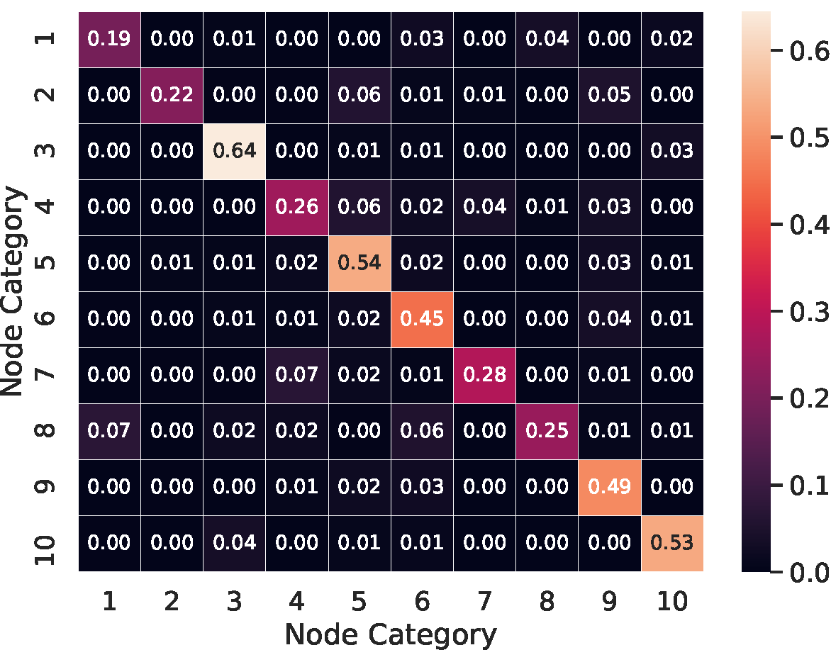
Figure 3. The category transition matrix on OGB-arXiv. To save space, we cut the number of categories to ten.

4.1. Experimental Settings

4.1.1. Dataset

For the full-supervised settings, we use the widely used benchmark dataset of citation network, OGB-arXiv (Hu et al., 2020a), which represents papers and their citation relations as nodes and edges, respectively. Each node has 128 features generated by averaging the embeddings of words in its title and abstract, where the embeddings are learned by the skip-gram model (Mikolov et al., 2013). Considering that the such old-fashioned text feature may not be representative, we replace the node features with a 768-dimensional vector extracted by feeding the title and abstract into RoBERTa (Liu et al., 2019) (12-layer ), where the representation of [CLS] token at the second last layer is selected.

For the semi-supervised settings, we adopt three widely used citation networks, Cora, Citeseer, and Pubmed, and select the 20-shot data split released by (Kipf and Welling, 2017), where 500 and 1000 nodes are selected as validation and testing, 20 nodes from each category are labeled for training. Apart from the real-world graphs, we further created three synthetic ones based on Citeseer by intentionally adding cross-category edges on 50% randomly selected nodes, which leads to local structure discrepancy between the poisoned nodes and the unaffected ones. Note that more cross-category edges lead to stronger discrepancy, making adaptive locality more critical for GCN models. In particular, according to the number of edges in the original Citeseer, we add 10%, 30%, and 50% of cross-category edges, constructing Citeseer(10%), Citeseer(30%), and Citeseer(50%). Note that the data split and node features are unchanged.

4.1.2. Compared Methods

To justify the proposed CGI, we compare it with the representative GCN, including GraphSAGE (Hamilton et al., 2017), GCN (Kipf and Welling, 2017), GAT (Veličković et al., 2018), JKNet (Xu et al., 2018), DAGNN (Liu et al., 2020), and APPNP (Klicpera et al., 2019), which adopts normal inference. Apart from GCN models, we also test MLP, which discard the graph structure and treat node classification as normal text classification. Lastly, as CGI uses two predictions, we include an ensemble baseline which averages the prediction of APPNP and MLP. For these models, we use the implementations on the OGB leaderboard. If necessary, e.g., under the transductive full-supervised setting, the hyper-parameters are tuned according to the settings in the original paper of the model. For the proposed CGI, we equipped the SVM with RBF kernel and apply CGI to APPNP. For the SVM, we tune two hyper-parameters $c$ and $\gamma$ through 5-fold cross-validation, i.e., splitting the nodes in validation into 5 folds. In addition, for the MCE that estimates graph uncertainty, we set the number of repeats and the edge dropout ratio $\tau$ as 50 and 0.15.

4.2. Effects of CGI (RQ1)

We first investigate to what extent the proposed CGI address the local structure discrepancy issue on the three synthetic datasets Citeseer(10%), Citeseer(30%), and Citeseer(50%). Table 1 shows the performance of APPNP, APPNP_Self, and APPNP_CGI on the three datasets, where the final prediction is the original prediction (i.e., $\hat{\bm{y}}$, the post-intervention prediction (i.e., $\hat{\bm{y}}^{s}$), and the final prediction from CGI (i.e., $\bar{\bm{y}}$), respectively. Note that the graph structure of the three datasets are different, the APPNP model trained on the datasets will thus be different. As such, the APPNP_Self will get different performance on the three datasets, while the node features are unchanged. From the table, we have the following observations:

• In all cases, APPNP_CGI outperforms APPNP, which validates the effectiveness of the proposed CGI. The performance gain is attributed to the further consideration of adaptive locality during GCN inference. In particular, the relative improvement over APPNP achieved by APPNP_CGI ranges from 1.1% to 7.2% across the three datasets. The result shows that CGI achieves large improvement over compared conventional one-pass GCN inference as more cross-category edges are injected, i.e., facing with more severe local structure discrepancy issue. The result further exhibits the capability of CGI to address the local structure discrepancy issue.

• As more cross-category edges being added, APPNP witnesses severe performance drop from the accuracy of 71.0% to 64.2%. This result is reasonable since GCN is vulnerable to cross-category edges which pushes the representations of node in different categories to be close (Chen et al., 2019b). Considering that APPNP has considered adaptive locality during model training, this result validates that adjusting the GCN architecture is insufficient to address the local structure discrepancy issue.

• As to APPNP_Self, the performance across the three datasets is comparable to each other. It indicates that the cross-category edges may not hinder the GCN to encode the association between target node features and the label. Therefore, the performance drop of APPNP when adding more cross-category edges is largely due to the improper neighbor aggregation without thorough consideration of the local structure discrepancy issue. Furthermore, on Citeseer(50%), the performance of APPNP_Self is comparable to APPNP, which indicates that the effect of considering adaptive locality during training is limited if the discrepancy is very strong.

4.3. Performance Comparison (RQ2)

To further verify the proposed CGI, we conduct performance comparison under both full-supervised and semi-supervised settings on the real-world datasets.

4.3.1. Semi-supervised setting.

We first investigate the effect of CGI under the semi-supervised setting by comparing the APPNP_CGI with APPNP, APPNP_Self, and APPNP_Ensemble. The four methods corresponds to four inference mechanisms: 1) conventional one-pass GCN inference (APPNP); 2) causal intervention without consideration of graph structure (APPNP_Self); 3) ensemble of APPNP and APPNP_Self (APPNP_Ensemble); and 4) the proposed CGI. Note that the four inference mechanisms are applied on the same APPNP model with exactly same model parameters. Table 2 shows the node classification performance on three real-world datasets: Cora, Citeseer, and Pubmed. From the table, we have the following observations:

• On the three datasets, the performance of APPNP_Self is largely worse than APPNP, i.e., omitting graph structure during GCN inference witnesses sharp performance drop under semi-supervised setting, which shows the importance of considering neighbors. Note that the performance of APPNP_Self largely surpasses the performance of MLP reported in (Kipf and Welling, 2017), which highlights the difference between performing causal intervention $do(N=\emptyset)$ on a GCN model and the inference of MLP which is trained without the consideration of graph structure.

• In all cases, APPNP_Ensemble performs worse than APPNP, which is one of the base models of the ensemble. The inferior performance of APPNP_Ensemble is mainly because of the huge gap between the performance of APPNP and APPNP_Self. From this results, we can conclude that, under semi-supervised setting, simply aggregating the original prediction and post-intervention prediction does not necessarily lead to better adaptive locality. Furthermore, the results validate the rationality of a carefully designed inference mechanism.

• In all cases, APPNP_CGI achieves the best performance. The performance gain is attributed to the choice model, which further validates the effectiveness of the proposed CGI. That is, it is essential to an inference model from the data, which accounts for the causal analysis of the original prediction. Moreover, this result reflects the potential of enhancing the inference mechanism of GCN for better decision making, especially the causality oriented analysis, which deserves further exploration in future research.

Dataset	Citeseer(10%)	Citeseer(30%)	Citeseer(50%)
APPNP	71.0%	64.4%	64.2%
APPNP_Self	65.1%	62.9%	64.3%
APPNP_CGI	71.8%	66.9%	68.6%
RI	1.1%	3.9%	7.2%

Table 1. Performance of APPNP’s original prediction, post-intervention prediction, and CGI prediction on the three synthetic datasets w.r.t. accuracy. RI means the relative improvement over APPNP achieved by APPNP_CGI.

Dataset	Cora	Citeseer	Pubmed
APPNP	81.8%	72.6%	79.8%
APPNP_Self	69.3%	66.5%	75.9%
APPNP_Ensemble	78.0%	71.4%	79.2%
APPNP_CGI	82.3%	73.7%	81.0%
RI	5.5%	2.8%	2.3%

Table 2. Performance of APPNP with different inference mechanisms on three semi-supervised node classification datasets w.r.t. the classification accuracy. RI means the relative improvement of APPNP_CGI over APPNP_Ensemble.

4.3.2. Full-supervised setting.

We then further investigate the effect of CGI under the full-supervised setting. Note that we test the models under both inductive and transductive settings on the OGB-arXiv dataset. As OGB-arXiv is a widely used benchmark, we also test the baseline methods. Table 3 shows the node classification performance of the compared methods on the OGB-arXiv dataset w.r.t. accuracy. Apart from the RoBERTa features, we also report the performance of baseline models with the original Word2Vec features. From the table, we have the following observations:

• The performance gap between MLP and GCN models will be largely bridged when replacing the Word2Vec features with the more advanced RoBERTa features. In particular, the relative performance improvement of GCN models over MLP shrinks from 27.9% to 3.7%. The result raises a concern that the merit of GCN model might be unintentionally exaggerated (Kipf and Welling, 2017) due to the low quality of node features.

• Moreover, as compared to APPNP, DAGNN performs better as using the Word2Vec features, while performs worse when using the RoBERTa features. It suggests accounting for feature quality in future research that investigates the capability of GCN or compares different GCN models.

• As to RoBERTa features, APPNP_Ensemble performs slightly better than its base models, i.e., APPNP_Self and APPNP. This result is different from the result in Table 2 under semi-supervised setting where the performance of APPNP_Self is inferior. We thus believe that improving the accuracy of the post-intervention prediction will benefit GCN inference (Zhou, 2012). As averaging the prediction of APPNP_Self and APPNP can also be seen as a choosing strategy by comparing model confidence, the performance gain indicates the benefit of considering adaptive locality during inference under full-supervised setting.

• APPNP_CGI further outperforms APPNP_Ensemble under both inductive and transductive settings, which is attributed to the choice model that learns to make choice from patterns of causal uncertainty, prediction confidence, and category transition factors. This result thus also shows the merit of characterizing the prediction of GCN models with the distilled factors.

• In all cases, the model achieves comparable performance under the inductive setting and the transductive setting. We postulate that the local structure discrepancy between training and testing nodes in the OGB-arXiv dataset is weak, which is thus hard for CGI to achieve huge improvements. In the following, the experiment is focused on the inductive setting which is closer to real-world scenarios that aim to serve the upcoming nodes.

4.4. In-depth Analysis (RQ3)

4.4.1. Effects of Distilled Factors

We then study the effects of the distilled factors as the inputs of the choice model in CGI. In particular, we compare the factors w.r.t. the performance of CGI as removing one factor in each round, where lower performance indicates larger contribution of the factor. Note that we report the accuracy regarding whether CGI makes the correct choice for testing nodes, rather than the accuracy for node classification. That is to say, here we only consider “conflict” testing nodes where the two inferences of CGI (i.e., APPNP and APPNP_Self) have different classifications. Figure 4 shows the performance on OGB-arXiv under the inductive setting, where 6,810 nodes among the 47,420 testing nodes are identified as the conflict nodes. We omit the results of other datasets under the semi-supervised setting for saving space, which have a close trend.

From the figure, we have the following observations: 1) Discarding any factor will lead to performance drop as compared to the case with all factors as inputs of the choice model (i.e., All factors). This result indicates the effectiveness of the identified factors on characterizing GCN predictions which facilitate making the correct choice. 2) Among the factors, removing self_conf and neighbor_conf leads to the largest performance drop, showing that the confidence of prediction is the most informative factor regarding the reliability of the prediction. 3) In all cases, the performance of CGI surpasses the Majority class, which always chooses the original GCN prediction, i.e., CGI degrades to the conventional one-pass inference. The result further validates the rationality of additionally considering adaptive locality during GCN inference, i.e., choosing between the original prediction and the post-intervention prediction without consideration of neighbors. Lastly, considering that the “conflict” nodes account for 14.4% in the testing nodes (6,810/47,420) and the accuracy of CGI’s choices is 66.53%, there is still a large area for future exploration.

Feature	Method	Inductive	Transductive
Word2Vec (128)	MLP	55.84%	55.84%
	GraphSAGE	71.43%	71.52%
	GCN	71.83%	71.96%
	GAT	71.93%	72.04%
	JKNet	72.25%	72.48%
	DAGNN	72.07%	72.09%
	APPNP	71.61%	71.67%
RoBERTa (768)	JKNet	75.59%	75.54%
	MLP	72.26%	72.26%
	DAGNN	74.93%	74.83%
	APPNP	75.74%	75.61%
	APPNP_Self	73.43%	73.38%
	APPNP_Ensemble	76.26%	75.86%
	APPNP_CGI	76.52%	76.07%

Table 3. Performance comparison under full-supervised settings. We use bold font and underline to highlight the best and second best performance under each setting.

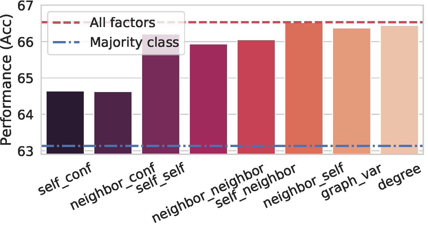
Figure 4. Illustration of factor influence on CGI.

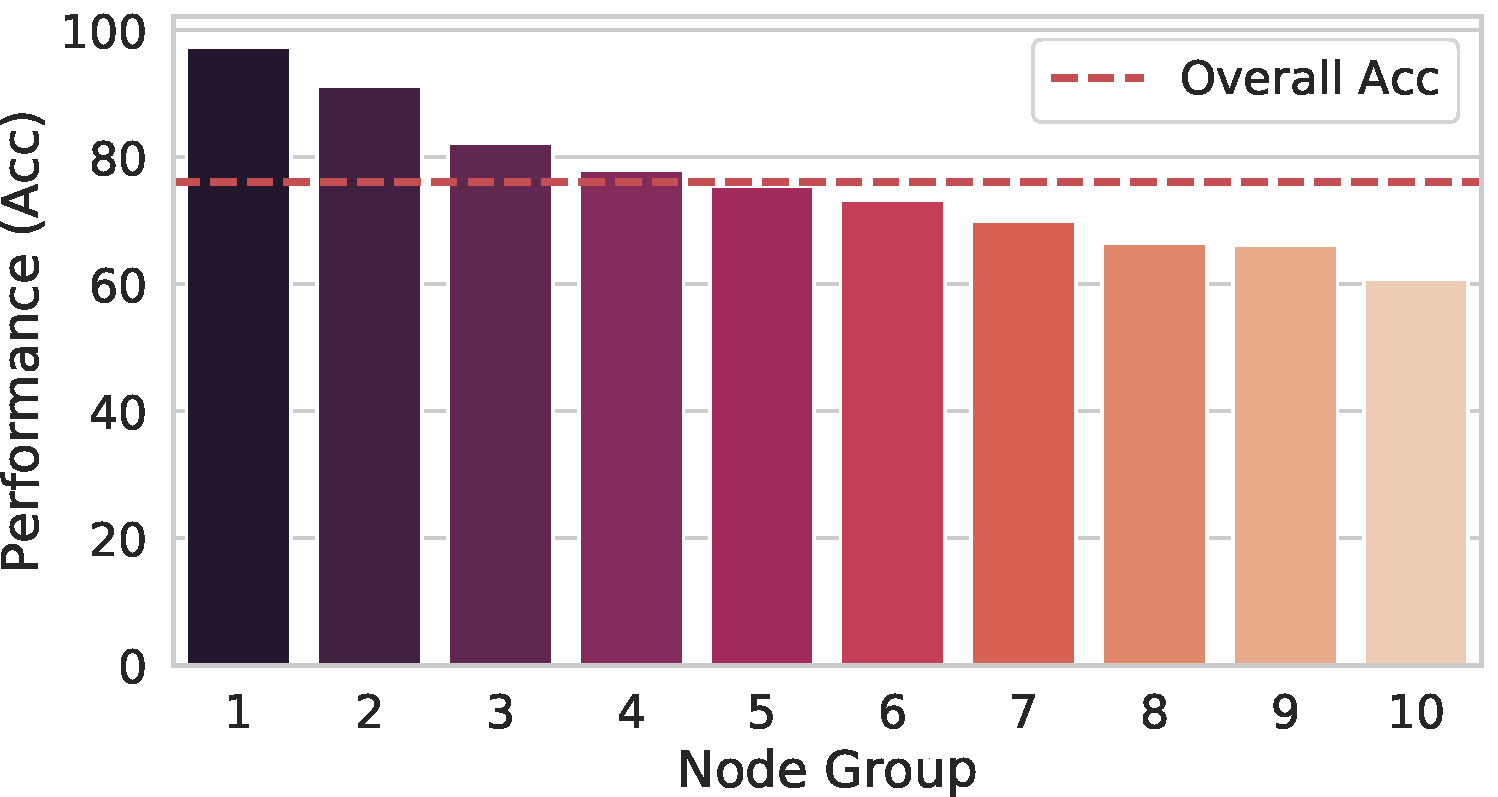
(a) MCE

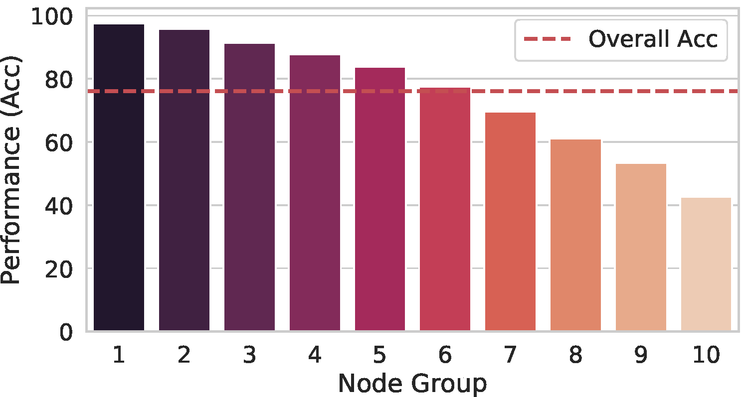
(b) Confidence (Conf)

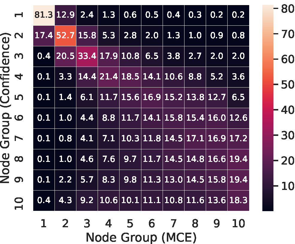
(c) Conf and MCE redundancy

Figure 5. Group-wise illustration of the causal uncertainty and the confidence of APPNP prediction, where MCE stands for the Monte Carlo causal effect uncertainty estimation (i.e., graph_var.)

4.4.2. Study on causal uncertainty.

Recall that we propose a Monte Carlo causal effect uncertainty (MCE) estimation to estimate the uncertainty of neighbors’ causal effect. We then investigate to what extent the MCE sheds light on the correctness of GCN prediction. Figure 5(a) shows the group-wise performance of APPNP on OGB-arXiv where the testing nodes are ranked according to the value of graph_var in an ascending order and split into ten groups with equal size. Note that we select OGB-arXiv for its relatively large scale where the testing set includes 47,420 nodes. From the figure, we can see a clear trend that the classification performance decreases as the MCE increases. It means that the calculated MCE is informative for the correctness of GCN predictions. For instance, a prediction has higher chance to be correct if its MCE is low.

As a reference, in Figure 5(b), we further depict the group-wise performance w.r.t. the prediction confidence (i.e., neighbor_conf). In particular, the testing nodes are ranked according to the value of neighbor_conf in a descending order. As can be seen, there is also a clear trend of prediction performance regarding the confidence, i.e., the probability of being correct is higher if APPNP is more confident on the prediction. To investigate whether MCE and GCN confidence are redundant, we further calculate the overlap ratio between the groups split by graph_var and the ones split by neighbor_conf. Figure 5(c) illustrates the matrix of overlap ratios. As can be seen, the weights are not dedicated on the diagonal entries. In particular, there are only two group pairs with overlap ratio higher than 0.5, which means that the MCE reveals the property of GCN prediction complementary to the confidence. That is, causal analysis indeed characterizes GCN predictions from distinct perspectives.

4.4.3. Training with trustworthiness signal

Model	APPNP	JKNet	DAGNN
Self+Neighbor	76.03	75.69	75.28
Self+Neighbor_Trust	78.30	75.71	78.61
Self+Neighbor_Bound	81.40	81.96	82.03

Table 4. Node classification performance of three GCN models: APPNP, JKNet, and DAGNN on OGB-arXiv.

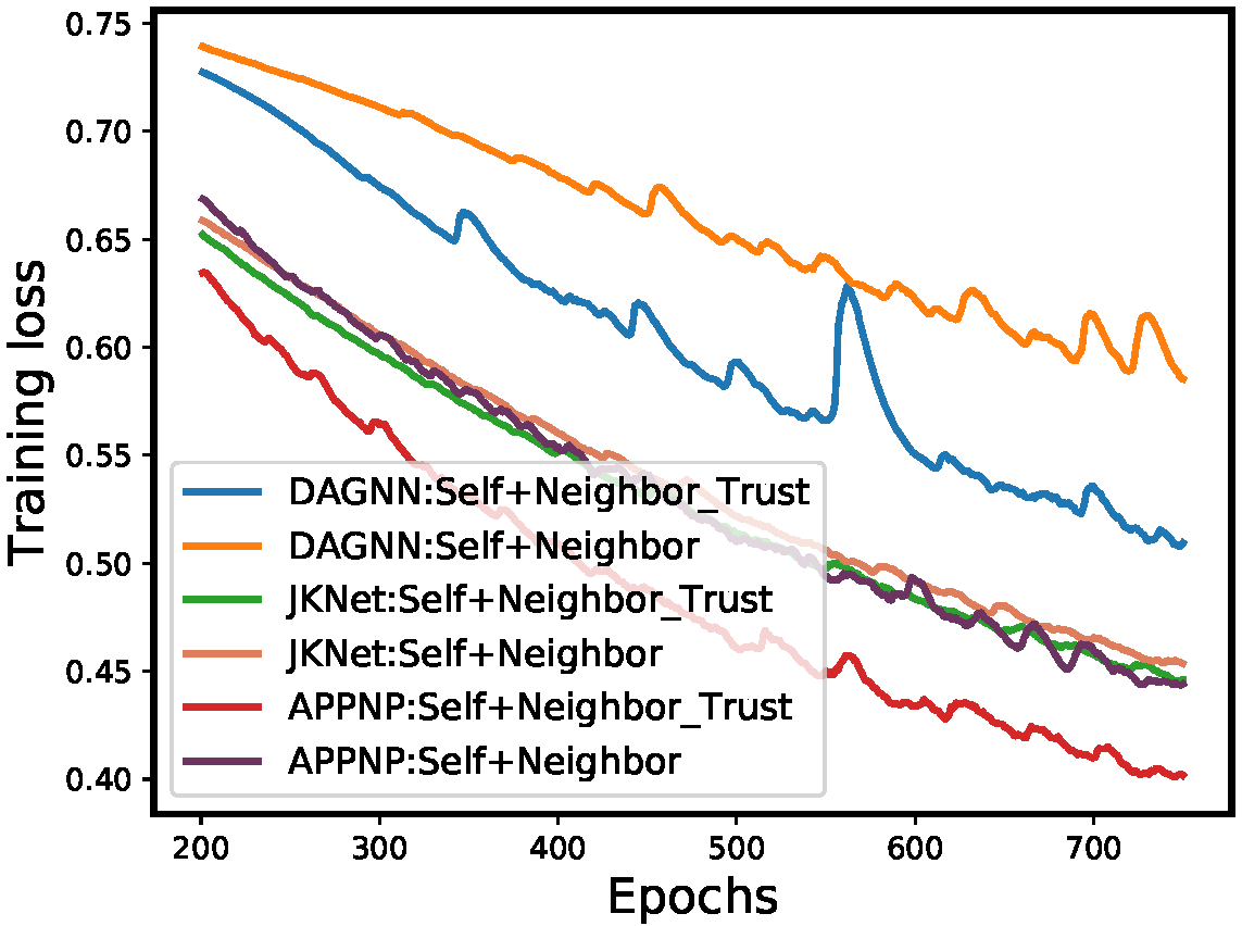
Figure 6. Training loss on OGB-arXiv under the Self+Neighbor and Self+Neighbor_Trust configurations.

To further investigate the benefit of performing adaptive locality during model inference, we further conduct a study on OGB-arXiv to test whether the GCN equipped with adaptive locality modules can really assess the trustworthiness of neighbors. Three representative GCN models with consideration of adaptive locality, APPNP, JKNet, and DAGNN, are tested under three different configurations:

• Self+Neighbor: This is the standard configuration of GCN model that accounts for the graph structure, i.e., trusting neighbors.

• Self+Neighbor_Trust: As compared to Self+Neighbor, a trustworthy feature is associated with each node, which indicates the “ground truth” of trusting self or neighbors. In particular, we train the GCN model, infer the original prediction and the post-intervention prediction, calculate the trustworthy feature according to Equation (10) (i.e., $p$). For the nodes where the original classification and the post-intervention classification are equal, we set the value as 0. By explicitly incorporating such value as a node feature, it should be easy for GCN to learn for properly performing adaptive locality if it works properly.

• As a reference, we study the GCNs in an ideal case, named Self+Neighbor_Bound, where the trustworthy feature is also given when performing adaptive locality during model inference.

Table 4 shows the model performance under the node classification setting of inductive full-supervised learning. From the table, we have the following observations:

• As compared to Self+Neighbor, all the three models, especially APPNP and DAGNN, achieve better performance under the configuration of Self+Neighbor_Trust. It indicates a better usage of the graph structure, which is attributed to the trustworthy feature. The result thus highlights the importance of modeling neighbor trustworthiness and performing adaptive locality.

• However, there is a large gap between Self+Neighbor_Trust and Self+Neighbor_Bound, showing the underuse of the trustworthy feature by the current adaptive locality methods. We postulate the reason to be the gap between the training objective, i.e., associating node representation with label, and the target of identifying trustworthy neighbors, which is the limitation of considering adaptive locality in model training. The performance under Self+Neighbor_Bound also reveals the potential of considering adaptive locality in model inference.

Furthermore, we study the impact of trustworthy feature on model training. Figure 6 illustrates the training loss along the training procedure of the tested GCNs under the configuration of Self+Neighbor and Self+Neighbor_Trust. It should be noted that we select the period from 200 to 750 epochs for better visualization. From the figure, we can see that, in all the three cases, the loss of GCN under Self+Neighbor_Trust is smaller than that under Self+Neighbor. The result shows that the trustworthy feature facilitates the GCN model fitting the training data, i.e., capturing the correlation between the node label and the node features as well as the graph structure. However, the adaptive locality module, especially graph attention, is distracted from the target of assessing neighbor trustworthiness. Theoretically, the graph attention can achieve the target by simply recognizing the value of the trustworthy feature from the inputs. For instance, the hop attention in DAGNN should highlight the target node representation at layer 0 if the trustworthy feature is 1.

5. Related Work

Graph Convolutional Network.

According to the format of the convolution operations, existing GCN models can be divided into two categories: spatial GCN and spectral GCN (Zhang et al., 2020a). Spectral GCN is defined as performing convolution operations in the Fourier domain with spectral node representations (Bruna et al., 2014; Defferrard et al., 2016; Kipf and Welling, 2017; Liao et al., 2019; Xu et al., 2019c). For instance, Bruna et al. (Bruna et al., 2014) perform convolution over the eigenvectors of graph Laplacian which are treated as the Fourier basis. Due to the high computational cost of the eigen-decomposition, a line of spectral GCN research has been focused on accelerating the eigen-decomposition with different approximation techniques (Defferrard et al., 2016; Kipf and Welling, 2017; Liao et al., 2019; Xu et al., 2019c). However, applying such spectral GCN models on large graphs still raises unaffordable memory cost, which hinders the their practical research.

To some extent, the attention on GCN research has been largely dedicated on the spatial GCN, which performs convolution operations directly over the graph structure by aggregating the features from spatially close neighbors to a target node (Atwood and Towsley, 2016; Hamilton et al., 2017; Kipf and Welling, 2017; Veličković et al., 2018; Xinyi and Chen, 2019; Veličković et al., 2019; Xu et al., 2019b). This line of research mainly focuses on the development of the neighbor aggregation operation. For instance, Kipf and Welling (Kipf and Welling, 2017) propose to use a linear aggregator (i.e., weighted sum) that uses the reverse of node degree as the coefficient. In addition to aggregating information from directly connected neighbors, augmented aggregators also account for multi-hop neighbors (Xu et al., 2019a; Jia et al., 2020). Moreover, non-linear aggregators are also employed in spatial GCNs such as capsule (Veličković et al., 2019) and Long Short-Term Memory (LSTM) (Hamilton et al., 2017). Besides, the general spatial GCN designed for simple graphs is extended to graphs with heterogeneous nodes (Wang et al., 2019b) and temporal structure (Park and Neville, 2019). Beyond model design, there are also studies on the model capability analysis (Xu et al., 2019b), model explanation (Ying et al., 2019), and training schema (Hu et al., 2020b).

However, most of the existing studies focus on the training stage and blindly adopt the one-pass forward propagation for GCN inference. This work is in an orthogonal direction, which improve the inference performance with an causal inference mechanism so as to better solve the local structure discrepancy issue. Moreover, to the best of our knowledge, this work is the first to introduce the causal intervention and causal uncertainty into GCN inference.

Adaptive Locality.

Amongst the GCN research, a surge of attention has been especially dedicated to solving the over-smoothing issue (Li et al., 2018). Adaptive locality has become the promising solution to alleviate the over-smoothing issue, which is typically achieved by the attention mechanism (Veličković et al., 2018; Xu et al., 2018; Wang et al., 2019b; Yun et al., 2019; Wang et al., 2020, 2019c; Chen et al., 2019a; Chen et al., 2020d) or residual connection (Kipf and Welling, 2017; Chen et al., 2020e; Li et al., 2020). Along the line of research on attention design, integrating context information into the calculation of attention weight is one of the most popular techniques. For instance, Wang et al.  (Wang et al., 2020) treats the neighbors at different hops as augmentation of attention inputs. Moreover, to alleviate the issue of lacking direct supervision, Wang et al.  (Wang et al., 2019c) introduce additional constraints to facilitate attention learning. Similar as Convolutional Neural Networks, residual connection has also been introduced to original design of GCN (Kipf and Welling, 2017), which connects each layer to the output directly. In addition to the vanilla residual connection, the revised versions are also introduced such as the pre-activation residual (Li et al., 2020) and initial residual (Chen et al., 2020e). Besides, the concept of inception module is also introduced to GCN model (Kazi et al., 2019), which incorporates graph convolutions with different receptive fields. For the existing methods, the adaptive locality mechanism is fixed once the GCN model is trained. Instead, this work explores adaptive locality during model inference, which is in an orthogonal direction.

Causality-aware Model Prediction.

A surge of attention is being dedicated to incorporating causality into the ML schema (Yang et al., 2021; Zhang et al., 2020c; Nan et al., 2021; Zhang et al., 2021; Yue et al., 2020; Hu et al., 2021). A line of research focuses on enhancing the inference stage of ML model from the cause-effect view (Yue et al., 2021; Wang et al., 2021; Niu et al., 2021; Tang et al., 2020a). This work differs from them for two reasons: 1) none of the existing work studies GCN; and 2) we learn a choice model to make final prediction from causal intervention results instead of performing a heuristic causal inference for making final prediction.

6. Conclusion

This paper revealed that learning an additional model component such as graph attention is insufficient for addressing the local structure discrepancy issue of GCN models. Beyond model training, we explored the potential of empowering the GCNs with adaptive locality ability during the inference. In particular, we proposed an causal inference mechanism, which leverages the theory of causal intervention, generating a post intervention prediction when the model only trusts own features, and makes choice between the post intervention prediction and original prediction. A set of factors are identified to characterize the predictions and taken as inputs for choosing the final prediction. Especially, we proposed the Monte Carlo estimation of neighbors’ causal effect. Under three common settings for node classification, we conducted extensive experiments on seven datasets, justifying the effectiveness of the proposed CGI.

In the future, we will test the proposed CGI on more GCN models such as GAT, JKNet, and DAGNN. Moreover, we will extend the proposed CGI from node classification to other graph analytic tasks, such as link prediction (Ren et al., 2017). In addition, following the original Monte Carlo estimation, we would like to complete the mathematical derivation of Equation 11, i.e., how the graph_var approximates the variance of the causal effect distribution. Lastly, we will explore how the property of the choice model $g(\cdot)$ influences the effectiveness of CGI, e.g., whether non-linearity is necessary.

References

- (1)
- Atwood and Towsley (2016) James Atwood and Don Towsley. 2016. Diffusion-convolutional neural networks. In NeurIPS. 1993–2001.
- Bruna et al. (2014) Joan Bruna, Wojciech Zaremba, Arthur Szlam, and Yann LeCun. 2014. Spectral networks and locally connected networks on graphs. ICLR (2014).
- Chen et al. (2020c) Deli Chen, Yankai Lin, Wei Li, Peng Li, Jie Zhou, and Xu Sun. 2020c. Measuring and Relieving the Over-smoothing Problem for Graph Neural Networks from the Topological View. AAAI (2020), 3438–3445.
- Chen et al. (2019b) Deli Chen, Xiaoqian Liu, Yankai Lin, Peng Li, Jie Zhou, Qi Su, and Xu Sun. 2019b. Improving Node Classification by Co-training Node Pair Classification: A Novel Training Framework for General Graph Neural Networks. arXiv preprint arXiv:1911.03904 (2019).
- Chen et al. (2020a) Jiawei Chen, Hande Dong, Xiang Wang, Fuli Feng, Meng Wang, and Xiangnan He. 2020a. Bias and Debias in Recommender System: A Survey and Future Directions. arXiv preprint arXiv:2010.03240 (2020).
- Chen et al. (2020d) Jingjing Chen, Liangming Pan, Zhipeng Wei, Xiang Wang, Chong-Wah Ngo, and Tat-Seng Chua. 2020d. Zero-shot ingredient recognition by multi-relational graph convolutional network. In Proceedings of the AAAI Conference on Artificial Intelligence, Vol. 34. 10542–10550.
- Chen et al. (2020e) Ming Chen, Zhewei Wei, Zengfeng Huang, Bolin Ding, and Yaliang Li. 2020e. Simple and deep graph convolutional networks. ICML (2020).
- Chen et al. (2020b) Ting Chen, Simon Kornblith, Kevin Swersky, Mohammad Norouzi, and Geoffrey Hinton. 2020b. Big self-supervised models are strong semi-supervised learners. arXiv preprint arXiv:2006.10029 (2020).
- Chen et al. (2019a) Weijian Chen, Yulong Gu, Zhaochun Ren, Xiangnan He, Hongtao Xie, Tong Guo, Dawei Yin, and Yongdong Zhang. 2019a. Semi-supervised User Profiling with Heterogeneous Graph Attention Networks. In IJCAI. 2116–2122.
- Defferrard et al. (2016) Michaël Defferrard, Xavier Bresson, and Pierre Vandergheynst. 2016. Convolutional neural networks on graphs with fast localized spectral filtering. In NeurIPS. 3844–3852.
- Hamilton et al. (2017) Will Hamilton, Zhitao Ying, and Jure Leskovec. 2017. Inductive representation learning on large graphs. In NeurIPS. 1024–1034.
- He et al. (2020) Xiangnan He, Kuan Deng, Xiang Wang, Yan Li, Yongdong Zhang, and Meng Wang. 2020. LightGCN: Simplifying and Powering Graph Convolution Network for Recommendation. In SIGIR.
- Hinton et al. (2015) Geoffrey Hinton, Oriol Vinyals, and Jeff Dean. 2015. Distilling the knowledge in a neural network. arXiv preprint arXiv:1503.02531 (2015).
- Hu et al. (2020c) Guangyi Hu, Chongyang Shi, Shufeng Hao, and Yu Bai. 2020c. Residual-Duet Network with Tree Dependency Representation for Chinese Question-Answering Sentiment Analysis. In Proceedings of the 43rd International ACM SIGIR Conference on Research and Development in Information Retrieval. 1725–1728.
- Hu et al. (2020a) Weihua Hu, Matthias Fey, Marinka Zitnik, Yuxiao Dong, Hongyu Ren, Bowen Liu, Michele Catasta, and Jure Leskovec. 2020a. Open graph benchmark: Datasets for machine learning on graphs. NeurIPS (2020).
- Hu et al. (2020b) Weihua Hu, Bowen Liu, Joseph Gomes, Marinka Zitnik, Percy Liang, Vijay S. Pande, and Jure Leskovec. 2020b. Strategies for Pre-training Graph Neural Networks. In ICLR.
- Hu et al. (2021) Xinting Hu, Kaihua Tang, Chunyan Miao, Xian-Sheng Hua, and Hanwang Zhang. 2021. Distilling Causal Effect of Data in Class-Incremental Learning. IEEE Conference on Computer Vision and Pattern Recognition (2021).
- Jia et al. (2020) Zhihao Jia, Sina Lin, Rex Ying, Jiaxuan You, Jure Leskovec, and Alex Aiken. 2020. Redundancy-Free Computation for Graph Neural Networks. In SIGKDD. 997–1005.
- Kazi et al. (2019) Anees Kazi, Shayan Shekarforoush, S Arvind Krishna, Hendrik Burwinkel, Gerome Vivar, Karsten Kortüm, Seyed-Ahmad Ahmadi, Shadi Albarqouni, and Nassir Navab. 2019. InceptionGCN: receptive field aware graph convolutional network for disease prediction. In International Conference on Information Processing in Medical Imaging. Springer, 73–85.
- Kipf and Welling (2017) Thomas N Kipf and Max Welling. 2017. Semi-supervised classification with graph convolutional networks. ICLR (2017).
- Klicpera et al. (2019) Johannes Klicpera, Aleksandar Bojchevski, and Stephan Günnemann. 2019. Predict then propagate: Graph neural networks meet personalized pagerank. ICLR (2019).
- Knyazev et al. (2019) Boris Knyazev, Graham W Taylor, and Mohamed Amer. 2019. Understanding Attention and Generalization in Graph Neural Networks. In NeurIPS. 4204–4214.
- Li et al. (2020) Guohao Li, Chenxin Xiong, Ali Thabet, and Bernard Ghanem. 2020. Deepergcn: All you need to train deeper gcns. arXiv preprint arXiv:2006.07739 (2020).
- Li et al. (2018) Qimai Li, Zhichao Han, and Xiao-Ming Wu. 2018. Deeper insights into graph convolutional networks for semi-supervised learning. In AAAI.
- Liao et al. (2019) Renjie Liao, Zhizhen Zhao, Raquel Urtasun, and Richard Zemel. 2019. LanczosNet: Multi-Scale Deep Graph Convolutional Networks. In ICLR.
- Linmei et al. (2019) Hu Linmei, Tianchi Yang, Chuan Shi, Houye Ji, and Xiaoli Li. 2019. Heterogeneous graph attention networks for semi-supervised short text classification. In EMNLP-IJCNLP. 4823–4832.
- Liu et al. (2020) Meng Liu, Hongyang Gao, and Shuiwang Ji. 2020. Towards Deeper Graph Neural Networks. In SIGKDD. 338–348.
- Liu et al. (2019) Yinhan Liu, Myle Ott, Naman Goyal, Jingfei Du, Mandar Joshi, Danqi Chen, Omer Levy, Mike Lewis, Luke Zettlemoyer, and Veselin Stoyanov. 2019. Roberta: A robustly optimized bert pretraining approach. arXiv e-prints (2019). arXiv:1907.11692
- Mao et al. (2020) Kelong Mao, Xi Xiao, Jieming Zhu, Biao Lu, Ruiming Tang, and Xiuqiang He. 2020. Item Tagging for Information Retrieval: A Tripartite Graph Neural Network based Approach. In Proceedings of the 43rd International ACM SIGIR Conference on Research and Development in Information Retrieval. 2327–2336.
- McPherson et al. (2001) Miller McPherson, Lynn Smith-Lovin, and James M Cook. 2001. Birds of a feather: Homophily in social networks. Annual review of sociology 27, 1 (2001), 415–444.
- Mikolov et al. (2013) Tomas Mikolov, Ilya Sutskever, Kai Chen, Greg S Corrado, and Jeff Dean. 2013. Distributed representations of words and phrases and their compositionality. In NeurIPS. 3111–3119.
- Nan et al. (2021) Guoshun Nan, Rui Qiao, Yao Xiao, Jun Liu, Sicong Leng, Hao Zhang, and Wei Lu. 2021. Interventional Video Grounding with Dual Contrastive Learning. In IEEE Conference on Computer Vision and Pattern Recognition.
- Niu et al. (2021) Yulei Niu, Kaihua Tang, Hanwang Zhang, Zhiwu Lu, Xian-Sheng Hua, and Ji-Rong Wen. 2021. Counterfactual vqa: A cause-effect look at language bias. IEEE Conference on Computer Vision and Pattern Recognition (2021).
- Park and Neville (2019) Hogun Park and Jennifer Neville. 2019. Exploiting interaction links for node classification with deep graph neural networks. In IJCAI. 3223–3230.
- Pearl (2009) Judea Pearl. 2009. Causality. Cambridge university press.
- Pearl (2019) Judea Pearl. 2019. The seven tools of causal inference, with reflections on machine learning. Commun. ACM 62, 3 (2019), 54–60.
- Pedregosa et al. (2011) Fabian Pedregosa, Gaël Varoquaux, Alexandre Gramfort, Vincent Michel, Bertrand Thirion, Olivier Grisel, Mathieu Blondel, Peter Prettenhofer, Ron Weiss, Vincent Dubourg, et al. 2011. Scikit-learn: Machine learning in Python. JMLR 12 (2011), 2825–2830.
- Ren et al. (2017) Zhaochun Ren, Shangsong Liang, Piji Li, Shuaiqiang Wang, and Maarten de Rijke. 2017. Social collaborative viewpoint regression with explainable recommendations. In Proceedings of the tenth ACM international conference on web search and data mining. 485–494.
- Rong et al. (2019) Yu Rong, Wenbing Huang, Tingyang Xu, and Junzhou Huang. 2019. Dropedge: Towards deep graph convolutional networks on node classification. In ICLR.
- Saito et al. (2018) Kuniaki Saito, Yoshitaka Ushiku, Tatsuya Harada, and Kate Saenko. 2018. Adversarial Dropout Regularization. In International Conference on Learning Representations.
- Tang et al. (2020a) Kaihua Tang, Jianqiang Huang, and Hanwang Zhang. 2020a. Long-Tailed Classification by Keeping the Good and Removing the Bad Momentum Causal Effect. Advances in Neural Information Processing Systems 33 (2020).
- Tang et al. (2020b) Xianfeng Tang, Huaxiu Yao, Yiwei Sun, Yiqi Wang, Jiliang Tang, Charu Aggarwal, Prasenjit Mitra, and Suhang Wang. 2020b. Investigating and Mitigating Degree-Related Biases in Graph Convoltuional Networks. In Proceedings of the 29th ACM International Conference on Information & Knowledge Management. 1435–1444.
- Vaswani et al. (2017) Ashish Vaswani, Noam Shazeer, Niki Parmar, Jakob Uszkoreit, Llion Jones, Aidan N Gomez, Łukasz Kaiser, and Illia Polosukhin. 2017. Attention is all you need. In NeurIPS. 5998–6008.
- Veličković et al. (2018) Petar Veličković, Guillem Cucurull, Arantxa Casanova, Adriana Romero, Pietro Lio, and Yoshua Bengio. 2018. Graph attention networks. ICLR (2018).
- Veličković et al. (2019) Petar Veličković, William Fedus, William L. Hamilton, Pietro Liò, Yoshua Bengio, and R Devon Hjelm. 2019. Deep Graph Infomax. In ICLR.
- Wang et al. (2019c) Guangtao Wang, Rex Ying, Jing Huang, and Jure Leskovec. 2019c. Improving graph attention networks with large margin-based constraints. arXiv preprint arXiv:1910.11945 (2019).
- Wang et al. (2020) Guangtao Wang, Rex Ying, Jing Huang, and Jure Leskovec. 2020. Direct Multi-hop Attention based Graph Neural Network. arXiv preprint arXiv:2009.14332 (2020).
- Wang et al. (2021) Wenjie Wang, Fuli Feng, Xiangnan He, Hanwang Zhang, and Tat-Seng Chua. 2021. ” Click” Is Not Equal to” Like”: Counterfactual Recommendation for Mitigating Clickbait Issue. Proceedings of the 44th International ACM SIGIR Conference on Research and Development in Information Retrieval (2021).
- Wang et al. (2019a) Xiang Wang, Xiangnan He, Meng Wang, Fuli Feng, and Tat-Seng Chua. 2019a. Neural Graph Collaborative Filtering. In SIGIR. 165–174.
- Wang et al. (2019b) Xiao Wang, Houye Ji, Chuan Shi, Bai Wang, Yanfang Ye, Peng Cui, and Philip S Yu. 2019b. Heterogeneous graph attention network. In WWW. 2022–2032.
- Xinyi and Chen (2019) Zhang Xinyi and Lihui Chen. 2019. Capsule Graph Neural Network. In ICLR.
- Xu et al. (2019c) Bingbing Xu, Huawei Shen, Qi Cao, Yunqi Qiu, and Xueqi Cheng. 2019c. Graph Wavelet Neural Network. In ICLR.
- Xu et al. (2019a) Chunyan Xu, Zhen Cui, Xiaobin Hong, Tong Zhang, Jian Yang, and Wei Liu. 2019a. Graph inference learning for semi-supervised classification. In ICLR.
- Xu et al. (2019b) Keyulu Xu, Weihua Hu, Jure Leskovec, and Stefanie Jegelka. 2019b. How Powerful are Graph Neural Networks? ICLR (2019).
- Xu et al. (2018) Keyulu Xu, Chengtao Li, Yonglong Tian, Tomohiro Sonobe, Ken-ichi Kawarabayashi, and Stefanie Jegelka. 2018. Representation learning on graphs with jumping knowledge networks. ICML (2018), 8676–8685.
- Yang et al. (2021) Xun Yang, Fuli Feng, Wei Ji, Meng Wang, and Tat-Seng Chua. 2021. Deconfounded Video Moment Retrieval with Causal Intervention. In Proceedings of the 44th International ACM SIGIR Conference on Research and Development in Information Retrieval.
- Yang (2020) Zuoxi Yang. 2020. Biomedical Information Retrieval incorporating Knowledge Graph for Explainable Precision Medicine. In Proceedings of the 43rd International ACM SIGIR Conference on Research and Development in Information Retrieval. 2486–2486.
- Ying et al. (2019) Zhitao Ying, Dylan Bourgeois, Jiaxuan You, Marinka Zitnik, and Jure Leskovec. 2019. Gnnexplainer: Generating explanations for graph neural networks. In NeurIPS. 9244–9255.
- Yue et al. (2021) Zhongqi Yue, Tan Wang, Hanwang Zhang, Qianru Sun, and Xian-Sheng Hua. 2021. Counterfactual Zero-Shot and Open-Set Visual Recognition. IEEE Conference on Computer Vision and Pattern Recognition (2021).
- Yue et al. (2020) Zhongqi Yue, Hanwang Zhang, Qianru Sun, and Xian-Sheng Hua. 2020. Interventional Few-Shot Learning. Advances in Neural Information Processing Systems 33 (2020).
- Yun et al. (2019) Seongjun Yun, Minbyul Jeong, Raehyun Kim, Jaewoo Kang, and Hyunwoo J Kim. 2019. Graph transformer networks. In NeurIPS. 11983–11993.
- Zhang et al. (2020c) Shengyu Zhang, Tan Jiang, Tan Wang, Kun Kuang, Zhou Zhao, Jianke Zhu, Jin Yu, Hongxia Yang, and Fei Wu. 2020c. DeVLBert: Learning Deconfounded Visio-Linguistic Representations. In Proceedings of the 28th ACM International Conference on Multimedia. 4373–4382.
- Zhang et al. (2021) Shengyu Zhang, Dong Yao, Zhou Zhao, Tat-Seng Chua, and Fei Wu. 2021. CauseRec: Counterfactual User Sequence Synthesis for Sequential Recommendation. In Proceedings of the 44th International ACM SIGIR Conference on Research and Development in Information Retrieval.
- Zhang et al. (2020b) Wenxuan Zhang, Yang Deng, and Wai Lam. 2020b. Answer ranking for product-related questions via multiple semantic relations modeling. In Proceedings of the 43rd International ACM SIGIR Conference on Research and Development in Information Retrieval. 569–578.
- Zhang et al. (2020a) Ziwei Zhang, Peng Cui, and Wenwu Zhu. 2020a. Deep learning on graphs: A survey. TKDE (2020).
- Zhou (2012) Zhi-Hua Zhou. 2012. Ensemble methods: foundations and algorithms. Chapman and Hall/CRC.