Spin-current version of solar cells in non-centrosymmetric magnetic insulators

Abstract

Photovoltaic effect, e.g., solar cells, converts light into DC electric current. This phenomenon takes place in various setups such as in noncentrosymmetric crystals and semiconductor pn junctions. Recently, we proposed a theory for producing DC spin current in magnets using electromagnetic waves, i.e., the spin-current counterpart of the solar cells. Our calculation shows that the nonlinear conductivity for the spin current is nonzero in a variety of noncentrosymmetric magnets, implying that the phenomenon is ubiquitous in inversion-asymmetric materials with magnetic excitations. Intuitively, this phenomenon is a bulk photovoltaic effect of magnetic excitations, where electrons and holes, visible light, and inversion-asymmetric semiconductors are replaced with magnons or spinons, THz or GHz waves, and asymmetric magnetic insulators, respectively. We also show that the photon-driven spin current is shift current type, and as a result, the current is stable against impurity scattering. This bulk photovoltaic spin current is in sharp contrast to that of well-known spin pumping that takes place at the interface between a magnet and a metal.

I Introduction

The technology based on electromagnetic waves and laser has long contributed to the development and discovery of photo-induced phenomena. Among them, the DC photocurrent in solar cells is a representative phenomenon Sturman and Fridkin (1992). The basic structure of solar cells is a junction of two different (p- and n-type) semiconductors. The point is that the inversion symmetry breaking is necessary to create a DC current by AC electromagnetic fields (see Appendix). Electromagnetic wave is merely an oscillating field and thereby it does not favor any spatial direction. Thus, the system (i.e., solar cell) should have a peculiar direction to induce electric current. Besides the pn junctions, single bulk crystals without inversion symmetry (i.e., noncentrosymmetric crystals), such as perovskite photovoltaics, have attracted attention as another platform of photovoltaic devices. The photocurrents in semiconductors Kohli et al. (2011); Cote et al. (2002); Sotome et al. (2019), transition-metal oxides Koch et al. (1976); Dalba et al. (1995) and organic materials Nakamura et al. (2017) have been experimentally observed, and the corresponding microscopic theories Kraut and von Baltz (1979); V. Belinicher and Sturman (1982); Sturman and Fridkin (1992); Král (2000); Sipe and Shkrebtii (2000) for photocurrents have been developed, especially, in recent years Young and Rappe (2012); Morimoto and Nagaosa (2016); Cook et al. (2017); Ishizuka and Nagaosa (2017). These phenomena are a consequence of the asymmetric optical transition of electrons.

Besides electrons, photo-induced dynamics has also been studied in various systems with different quasi particles such as ferro and antiferromagnets Kirilyuk et al. (2010); Němec and Kimel (2018). However, the optical control of the flow of these quasi particles has not been studied so far. In this work, we explored one such example in magnetic insulators, i.e., an optical generation of magnon or spinon flow in magnetic materials Ishizuka and Sato (2019a, b). Since magnons and spinons are magnetic excitations carrying angular momentum, the photovoltaic magnon/spinon current is the spin-current version of photocurrent.

Spin current Maekawa et al. (2012) is defined as the flow of angular momentum and have been continuously a hot topic in spintronics. It can be viewed as a new instrument of information processing besides usual electric current, and several methods of creating/controlling spin current have been proposed and realized. Moreover, spin current has gathered attention as an important element of novel transport phenomena from the viewpoint of fundamental science.

Intense terahertz (THz) or gigahertz (GHz) waves are efficient to create DC photo spin current in magnetic insulators because energies of magnetic excitations with spin angular momentum (i.e., carriers of spin current) are usually located in THz or GHz range. The THz-laser science has massively progressed in recent years, and now we can utilize strong THz laser pulse Hirori et al. (2011); Sato et al. (2013); Liu et al. (2017) whose AC-electric-field strength is beyond 1 MV/cm ($\sim$ 0.1-1T of AC magnetic field) in the range of 0.1-10 THz. Actually, several THz-laser (wave) driven magnetic phenomena have been actively studied. For instance, THz-wave driven magnetic resonance Mukai et al. (2016); Baierl et al. (2016); Kubacka et al. (2014), a magnetic-excitation mediated high harmonic generation Lu et al. (2017) with THz laser, etc. have been observed. Microscopic theories Takayoshi et al. (2014a, b); Sato et al. (2016); Fujita and Sato (2017); Ikeda and Sato (2019); Sato and Morisaku (2020) for THz-wave driven magnetic phenomena have also been developed recently. Similar technologies using THz waves apply to the photovoltaic spin current as well.

This proceedings discusses the essential aspects of photo-generation of spin current in magnetic insulators. As shown in Table 1, noncentrosymmetric semiconductors, electrons (or holes), and visible or infrared waves are replaced with noncentrosymmetirc magnets, magnetic excitations (magnons, spinons etc.), and GHz/THz waves in our proposal Ishizuka and Sato (2019a, b).

Table 1: Set ups of solar cell of creating electric current and our proposal of doing spin current.

Solar cell	Our proposal (spin-current version of solar cell)
Noncentrosymmetric semiconductors	Noncentrosymmetric magnetic insulators
Infrared or visible light (1THz-1PHz)	GHz or THz waves (0.1-10THz)
Electrons and holes	Magnetic excitations (magnons, spinons, etc.)

II Modeling

In this section, we define our models for photo-induced spin current. As we discussed in the previous section, inversion-asymmetric systems are necessary to create the photo spin current. To this end, we consider two kinds of quantum spin models as simple, but realistic magnetic systems.

II.1 Quantum Spin Chains

First, we consider an inversion-asymmetric quantum spin chain Giamarchi (2003); A. O. Gogolin and Tsvelik (2004); Tsvelik (2007) whose Hamiltonian is given by

$$H_{\rm 1D}= \sum_{j}J(1+(-1)^{j}\delta)(S_{j}^{x}S_{j+1}^{x}+S_{j}^{y}S_{j+1}^{y})-\sum_{j}(h+(-1)^{j}h_{s})S_{j}^{z},$$ (1)

where $S_{j}^{x,y,z}$ are $S=\frac{1}{2}$ spin operators on $j$th site ($\hbar$ is set to be unity), $J$ is the easy-plane exchange coupling whose energy scale is usually in GHz or THz regime, and $h$ is the external, uniform magnetic field along the $z$ axis. In general, two kinds of inversion symmetries exist in lattice systems: Bond-centered and site-centered inversion symmetries. The dimerization parameter $\delta$ violates the site-centered inversion symmetry, while the staggered field $h_{s}$ breaks the bond-centered one. A finite dimerization often occurs in low-dimensional systems with Peierls instability Giamarchi (2003), and a staggered field $h_{s}$ is known to emerge in a class of quasi one-dimensional (1D) magnets with low crystal symmetry Dender et al. (1997); Oshikawa et al. (1999); Feyerherm et al. (2000); Umegaki et al. (2009); Affleck and Oshikawa (1999). In addition, if we consider weakly coupled spin chains, a focused spin chain can be approximated by an 1D model subject to a staggered field due to the Néel order Scalapino et al. (1975); Schulz (1996); Sato and Oshikawa (2004); Okunishi and Suzuki (2007); Ishimura and Shiba (1980); Coldea et al. (2010) of neighboring chains. The model (1) is depicted in Fig. 1(a).

The 1D model (1) is exactly fermionized through Jordan-Wigner (JW) transformation Giamarchi (2003); A. O. Gogolin and Tsvelik (2004); Tsvelik (2007) . By introducing fermion operators $f_{j}=e^{-i\pi\sum_{\ell=1}^{j-1}S_{j}^{+}S_{j}^{-}}S_{j}^{-}$ and $f_{j}^{\dagger}=S_{j}^{+}e^{i\pi\sum_{\ell=1}^{j-1}S_{j}^{+}S_{j}^{-}}$ with $S^{\pm}_{j}=S_{j}^{x}\pm iS_{j}^{y}$, Eq. (1) is mapped to

$$H_{\rm 1D}=\sum_{j} \frac{J}{2}(1+(-1)^{j}\delta)\left(f_{j+1}^{\dagger}f_{j}+f_{j}^{\dagger}f_{j+1}\right)+(h+(-1)^{j}h_{s})n_{j},$$ (2)

where $n_{j}=f_{j}^{\dagger}f_{j}$ is the number operator on $j$th site. The mapped model (2) is a 1D tight-binding model of the spinless fermion. Its energy bands are shown in Fig. 1(b) and (c). We have a gapless energy dispersion in the inversion-symmetric case with $\delta=h_{s}=0$, as shown in Fig. 1(b), while a gap opens and valence and conducting bands appears if we introduce an inversion-asymmetric perturbation $\delta\neq 0$ or $h_{s}\neq 0$. When the magnetic field $h$ is small enough, the ground state of the spin chain (1) corresponds to the half-filled state of the fermion model (2). We will focus on the half-filled ground state in the rest of this paper. Since Eq. (2) is viewed as a model of an 1D spinless semiconductor, we can take analogy between the photo spin current and usual photo electric current in order to study the former of the spin chain. However, we should note that the fermions $f_{j}$ and $f_{j}^{\dagger}$ represent magnetic excitations (not electron) in the spin chain. Hereafter, we will call the JW fermions spinons for simplicity.

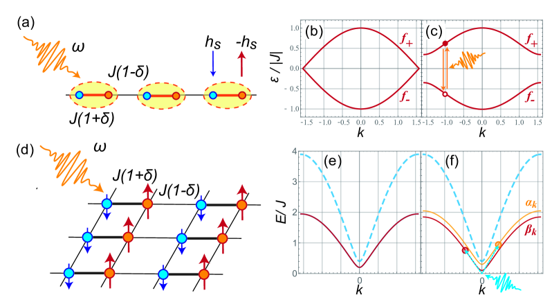
Figure 1: (a) Noncentrosymmetric quantum spin chain model and (d) noncentrosymmetric antiferromagnetic (or ferrimagnetic) insulator model. In the spin chain (a), a dimerization $\delta$ and a staggered field $h_{s}$ break the site- and bond-centered inversion symmetries, respectively. In the antiferromagnet (d), a dimerization $\delta$ and the ordering structure respectively break the site- and bond-centered inversion symmetries. Panels (b) and (c) represent the band dispersion of the JW fermion (here we call it spinon) for inversion-symmetric and asymmetric spin chains, respectively. Panels (e) and (f) depict the $\hat{x}$-direction magnon bands of the antiferromagnetic insulator models with $h_{+}=0$ and $h_{+}\neq 0$, respectively. For simplicity, we take the 1D limit $J_{\perp}/J\to 0$. The dotted blue curve correspond to $E_{\alpha}(\textit{{k}})+E_{\beta}(\textit{{k}})$.

II.2 Antiferromagnetic or Ferrimagnetic Insulators

Secondly, we consider the three-dimensional (3D) spin model with antiferro or ferrimagnetically ordered ground state. The model is shown in Fig. 1(d). The Hamiltonian is given by

$$H_{\rm 3D}= \sum_{\textit{{r}}}J(1+\delta)\textit{{S}}_{a}(\textit{{r}})\cdot\textit{{S}}_{b}(\textit{{r}})+J(1-\delta)\textit{{S}}_{a}(\textit{{r}}+\hat{x})\cdot\textit{{S}}_{b}(\textit{{r}})-(D+D_{s})\left[S_{a}^{z}(\textit{{r}})\right]^{2}-(D-D_{s})\left[S_{b}^{z}(\textit{{r}})\right]^{2}$$

$$-J_{\perp}\Big{[}\textit{{S}}_{a}(\textit{{r}})\cdot\textit{{S}}_{a}(\textit{{r}}+\hat{y})+\textit{{S}}_{a}(\textit{{r}})\cdot\textit{{S}}_{a}(\textit{{r}}+\hat{z})+\textit{{S}}_{b}(\textit{{r}})\cdot\textit{{S}}_{b}(\textit{{r}}+\hat{y})+\textit{{S}}_{b}(\textit{{r}})\cdot\textit{{S}}_{b}(\textit{{r}}+\hat{z})\Big{]}$$

$$-B\Big{[}g_{a}S_{a}^{z}(\textit{{r}})+g_{b}S_{b}^{z}(\textit{{r}})\Big{]}.$$ (3)

Here, $\textit{{S}}_{a(b)}(\textit{{r}})$ is the spin-$S_{a(b)}$ operator on rth site on $a(b)$ sublattice, where $\textit{{r}}=(m_{x}\hat{x},m_{y}\hat{y},m_{z}\hat{z})$ with $m_{x,y,z}$ being an integer and $\hat{a}$ ($a=x,y,z$) is the unit vector along the $a$ direction. $J$ is the antiferromagnetic exchange coupling constant along the $x$ direction and $J_{\perp}$ is the ferromagnetic constant along $y$ and $z$ directions. The parameter $\delta$ shows the dimerization on the $J$ bond. We have introduced uniform [staggered] single-ion anisotropy with $D>0$ [$D_{s}(<D)$] to stabilize the antiferromagnetic ordering. The final term of Eq. (3) is the Zeeman interaction induced by a uniform magnetic field $B$, and $g_{a}$ and $g_{b}$ respectively denote g factors on $a$ and $b$ sublattices. The ground state of the model (3) is Néel ordered for $S_{a}=S_{b}$ and ferrimagnetically ordered for $S_{a}\neq S_{b}$, as shown in Fig. 1(d). These antiferromagnetically ordering patterns break the bond-centered inversion symmetry even without a staggered anisotropy $D_{s}$ or a difference of g factors $g_{a}-g_{b}$. This is in contrast with the case of the 1D model (1), where a staggered field $h_{s}$ is necessary to lead to the breakdown of the bond-centered inversion symmetry. On the other hand, the dimerization $\delta$ breaks the site-centered inversion symmetry of Eq. (3) like the 1D case.

We can apply the spin-wave theory Yoshida (1996); Mattis (2006) for the antiferromagnetically ordered state of Eq. (3). Through the following Holstein-Primakoff transformation,

$$S_{a}^{z}(\textit{{r}})=S_{a}-n_{a}(\textit{{r}}),\,\,\,\,\,\,\,\,S_{a}^{+}(\textit{{r}})=\sqrt{2S_{a}}\left(1-\frac{n_{a}(\textit{{r}})}{2S_{a}}\right)^{\frac{1}{2}}a(\textit{{r}}),\,\,\,\,\,\,\,\,S_{a}^{-}(\textit{{r}})=\sqrt{2S_{a}}a^{\dagger}(\textit{{r}})\left(1-\frac{n_{a}(\textit{{r}})}{2S_{a}}\right)^{\frac{1}{2}},$$ (4)

$$S_{b}^{z}(\textit{{r}})=n_{b}(\textit{{r}})-S_{b},\,\,\,\,\,\,\,\,S_{b}^{+}(\textit{{r}})=\sqrt{2S_{b}}b^{\dagger}(\textit{{r}})\left(1-\frac{n_{b}(\textit{{r}})}{2S_{b}}\right)^{\frac{1}{2}},\,\,\,\,\,\,\,\,S_{b}^{-}(\textit{{r}})=\sqrt{2S_{b}}\left(1-\frac{n_{b}(\textit{{r}})}{2S_{b}}\right)^{\frac{1}{2}}b(\textit{{r}}),$$ (5)

the spin model (3) is mapped to a boson model. Here, $a(\textit{{r}})$ and $b(\textit{{r}})$ are respectively the bosonic annihilation operators at rth site on $a$ and $b$ sublattices. $n_{a}(\textit{{r}})=a^{\dagger}(\textit{{r}})a(\textit{{r}})$ and $n_{b}(\textit{{r}})=b^{\dagger}(\textit{{r}})b(\textit{{r}})$ are the number operators. Within the linear spin-wave approximation, the bosonized Hamiltonian is given by

$$H_{\rm 3D}\approx H_{\rm sw}=\sum_{\textit{{k}}}\left(\begin{array}[]{c}a_{\textit{{k}}}\\ b_{-\textit{{k}}}^{\dagger}\end{array}\right)^{\dagger}\left(\begin{array}[]{cc}h^{0}_{\textit{{k}}}+h^{z}_{\textit{{k}}}&h^{x}_{\textit{{k}}}-{\rm i}h^{y}_{\textit{{k}}}\\ h^{x}_{\textit{{k}}}+{\rm i}h^{y}_{\textit{{k}}}&h^{0}_{\textit{{k}}}-h^{z}_{\textit{{k}}}\end{array}\right)\left(\begin{array}[]{c}a_{\textit{{k}}}\\ b_{-\textit{{k}}}^{\dagger}\end{array}\right)+\text{const.}$$ (12)

Here, $h^{0,x,y,z}_{\textit{{k}}}$ are functions of wave vector k and parameters in Eq. (3), and we have introduced the Fourier transformation of Holstein-Primakoff bosons as $a_{\textit{{k}}}=(1/\sqrt{N})\sum_{\textit{{r}}}a(\textit{{r}})e^{{\rm i}\textit{{k}}\cdot\textit{{r}}}$ and $b_{\textit{{k}}}=(1/\sqrt{N})\sum_{\textit{{r}}}b(\textit{{r}})e^{{\rm i}\textit{{k}}\cdot(\textit{{r}}+\hat{x}/2)}$, where $N$ is the total site number of $a$ or $b$ sublattice. For this bilinear bosonic model, performing the following Bogoliubov transformation,

$$a_{\textit{{k}}}=\cosh\Theta_{\textit{{k}}}\alpha_{\textit{{k}}}+\sinh\Theta_{\textit{{k}}}\beta^{\dagger}_{-\textit{{k}}},\,\,\,\,\, b_{-\textit{{k}}}^{\dagger}=\sinh\Theta_{\textit{{k}}}e^{i\Phi_{\textit{{k}}}}\alpha_{\textit{{k}}}+\cosh\Theta_{\textit{{k}}}e^{i\Phi_{\textit{{k}}}}\beta_{-\textit{{k}}}^{\dagger},$$ (13)

we arrive at the diagonalized Hamiltonian,

$$H_{\rm sw}= \sum_{\textit{{k}}}E_{\alpha}(\textit{{k}})\alpha_{\textit{{k}}}^{\dagger}\alpha_{\textit{{k}}}+E_{\beta}(\textit{{k}})\beta_{\textit{{k}}}^{\dagger}\beta_{\textit{{k}}}+\text{const.}$$ (14)

Here, $\alpha_{\textit{{k}}}$ and $\beta_{\textit{{k}}}$ are annihilation operators of new bosons (i.e., magnons). When $h_{+}=D(S_{a}+S_{b}-1)+D_{s}(S_{a}-S_{b})-B(g_{a}-g_{b})/2=0$, energy dispersions of two magnons $\alpha_{\textit{{k}}}$ and $\beta_{\textit{{k}}}$ are degenerate as shown in Fig. 1(e). For $h_{+}\neq 0$, the band degeneracy is lifted as in Fig. 1(f).

II.3 Spin-light couplings

Let us consider the spin-light coupling to discuss the photo-induced spin current. In vacuum, the fundamental interaction between electron spins and electromagnetic fields is the Zeeman coupling. However, additional spin-light couplings may emerge in materials through complex interactions among light and matter fields.

For the spin chain model (2), we consider the following three sorts of spin-light couplings.

$$H_{\text{Z}}= -B(t)\sum_{j}(\eta-(-1)^{j}\eta_{s})S_{j}^{z}.$$ (15)

$$H_{\text{iDM}}= E_{y}(t)\sum_{j}(p+(-1)^{j}p_{s})\left(\textit{{S}}_{j}\times\textit{{S}}_{j+1}\right)^{z}.$$ (16)

$$H_{\text{ms}}=E_{x}(t)\sum_{j}(A+(-1)^{j}A_{s})(S_{j}^{x}S_{j+1}^{x}+S_{j}^{y}S_{j+1}^{y}).$$ (17)

Equation (15) represents an AC Zeeman coupling with $B(t)$ being the AC magnetic field of an applied electromagnetic wave. Here, we assume that the AC field $B(t)$ is parallel to the $S^{z}$ direction, i.e., longitudinal. The remaining two terms of Eqs. (16) and (17) are sorts of magnetoelectric couplings Tokura et al. (2014). Equation (16) is called an AC inverse Dyzaloshinskii-Moriya (iDM) interaction Tokura et al. (2014); Katsura et al. (2005) and it often appears in multiferroic magnets, in which electric polarization is strongly coupled to electron spins. The spin chain is located along the $x$ direction and $E_{\alpha}(t)$ is the $\alpha$ component of the AC electric field of an applied wave. Equation (17) is called an magnetostriction (MS) type interaction Tokura et al. (2014), where the AC electric field is coupled to the local magnetic exchange interaction. A typical origin of Eq. (17) is the spin-phonon coupling. Since we focus on inversion-asymmetric spin chains, we have introduced both uniform and staggered coupling constants in all the spin-light couplings such as $\eta$ and $\eta_{s}$.

For the antiferromagnetic model (3), we consider a standard AC Zeeman coupling,

$$H_{\text{Z,3D}}= -B(t)\sum_{\textit{{r}}}\Big{[}g_{a}S^{z}_{a}(\textit{{r}})+g_{b}S^{z}_{b}(\textit{{r}})\Big{]}$$ (18)

We set the AC magnetic field to be parallel to the $S^{z}$ direction like the 1D case.

We note that the $z$ component of total spin $S_{\rm tot}^{z}=\sum_{j}S_{j}^{z}$ (or $=\sum_{\textit{{r}}}S^{z}_{a}(\textit{{r}})+S^{z}_{b}(\textit{{r}})$) is conserved in all of our spin-light couplings. It means that the angular momentum transfer from photons to spins does not take place in our models. Nevertheless, as we will see soon later, an DC spin current is produced through these spin-light couplings. As one sees from Eqs. (15)-(18), we also note that we focus on simple linearly-polarized electromagnetic waves in this study.

III Second-order Response Theory and Results

In the previous section, we have explained our setup of generating photo-induced spin current. This section is devoted to showing our theoretical approach and results.

III.1 Second-order Response

The leading term of the DC response to an external AC field emerges from the second-order perturbation of the AC field (see Appendix). To calculate the DC spin current in our driven magnetic models, we apply the second-order response theory Kraut and von Baltz (1979); V. Belinicher and Sturman (1982); Král (2000); Sipe and Shkrebtii (2000) that is a standard extension of the well-known linear-response theory (i.e., Kubo formula). It is based on the perturbation expansion of the equation of motion for density matrices with respect to an applied AC field. Let us represent the AC perturbation term as $H^{\prime}(t)=F(t){\cal O}(t)$, where $F(t)$ is the external AC field and ${\cal O}(t)$ is an operator of the system we consider. According to the second-order response theory, the response of a current $I(t)$ is computed as

$$\langle I(t)\rangle_{2}= -\int_{0}^{\infty}dt_{1}dt_{2}\Big{\langle}[{\cal O}(t-t_{1}-t_{2}),\,\,[{\cal O}(t-t_{1}),\,\,I(t)]]\Big{\rangle}F(t-t_{1}-t_{2})F(t-t_{1}),$$ (19)

where $\langle\cdots\rangle_{2}$ stands for the second-order response. When the Fourier transformation along time $t$ is defined as $\langle I(\omega)\rangle_{2}=\int dt\langle I(t)\rangle_{2}e^{-i\omega t}$, Eq. (19) is transformed to

$$\langle I(\Omega)\rangle_{2}= \int d\omega\sigma^{(2)}(\Omega;\omega,\Omega-\omega)F(\omega)F(\Omega-\omega).$$ (20)

This equation defines the nonlinear conductivity $\sigma^{(2)}(\Omega;\omega,\Omega-\omega)$. If we apply this formula to electric current $I(t)$ of an 1D non-interacting electron system, the nonlinear DC conductivity ($\Omega=0$) is calculated as

$$\sigma^{(2)}(0;\omega,-\omega)= \sum_{\alpha,\beta,\gamma}\int\frac{dk}{(2\pi)^{2}}\frac{[f_{\alpha}(k)-f_{\beta}(k)]{\cal O}_{\alpha\beta}(k)}{\omega-\varepsilon_{\beta}(k)+\varepsilon_{\alpha}(k)-i/(2\tau)}\left[\frac{{\cal O}_{\beta\gamma}(k)I_{\gamma\alpha}(k)}{\varepsilon_{\alpha}(k)-\varepsilon_{\gamma}(k)-i/(2\tau)}-\frac{I_{\beta\gamma}(k){\cal O}_{\gamma\alpha}(k)}{\varepsilon_{\gamma}(k)-\varepsilon_{\beta}(k)-i/(2\tau)}\right],$$ (21)

where ${\cal O}_{\alpha\beta}(k)=\left\langle\alpha k\right|{\cal O}\left|\beta k\right\rangle$ and $I_{\alpha\beta}(k)=\left\langle\alpha k\right|I\left|\beta k\right\rangle$. where $|\alpha k\rangle$ is the electron energy eigenstate with wave number $k$ on the $\alpha$ band. $\epsilon_{\alpha}(k)$ is the eigen energy of the state $|\alpha k\rangle$, and $f_{\alpha}(k)=1/(1+e^{\epsilon_{\alpha}(k)/(k_{B}T)})$ is the fermion distribution function for $|\alpha k\rangle$. We have introduced a phenomenological relaxation time $\tau$ which is important to obtain a physically meaningful value of the conductivity $\sigma^{(2)}$. Note that $\sigma^{(2)}$ is ill-defined in the case of $1/\tau=0$.

III.2 Nonlinear Conductivity of Spin Current

We can straightforwardly apply the formula (21) to the photo-induced spin current in our spin chain model because the Hamiltonian is mapped to a non-interacting JW-fermion (spinon) form (2). The spin current with $S^{z}$ polarization may be defined from the equation of motion for the $z$ component of total spin. The resultant current is

$$J_{\rm sc}= \frac{1}{N_{\rm 1D}}\sum_{j}-J\left[1+(-1)^{j}\delta\right](S_{j}^{x}S_{j+1}^{y}-S_{j}^{y}S_{j+1}^{x}),$$ (22)

where $N_{\rm 1D}$ is the total site number. Therefore, the real part of the DC nonlinear conductivity is calculated as

$${\rm Re}[\sigma^{(2)}(0;\omega,-\omega)]= \frac{1}{\pi}{\rm Re}\left\{\sum_{k}\frac{{\cal O}_{+-}(k)J_{-+}(k)[{\cal O}_{--}(k)-{\cal O}_{++}(k)]}{\omega^{2}-[\varepsilon_{+}(k)-\varepsilon_{-}(k)-i/(2\tau)]^{2}}\right\},$$ (23)

where $\epsilon_{-}(k)$ and $\epsilon_{+}(k)$ are respectively the valence and conduction band dispersions [see Fig. 1(c)]. $J_{\alpha\beta}(k)$ is the matrix element of the spin current $J_{\rm sc}$, and ${\cal O}_{\alpha\beta}(k)$ is the matrix element of the operator part of the spin-light coupling [see Eqs. (15)-(17)]. We note that the imaginary part of the conductivity is zero for linearly polarized waves. Figure 2(a)-(c) represent the DC nonlinear conductivity of spin current in the inversion-asymmetric spin chain model Ishizuka and Sato (2019a) with different spin-light couplings at $k_{B}T=0$. We have set $1/\tau\to+0$ in Fig. 2. Three panels (a)-(c) show that a finite nonlinear conductivity occurs for all of the three spin-light couplings when the frequency $\omega$ is in the range of the energy difference between valence and conducting bands, i.e., when particle-hole pair creation is possible via the photon absorption [see Fig. 1(c)]. This frequency is usually in GHz or THz regime since the JW-fermion band width is mainly determined by the exchange couplings. We verify that the conductivity $\sigma^{(2)}$ vanishes unless both the site- and bond-centered symmetries are broken. In the case of AC Zeeman interaction or MS one with $A_{s}\neq 0$ [panels (b) and (c)], the conductivity $\sigma^{(2)}$ diverges near the lowest and highest frequencies $\omega$. This behavior stems from the divergent nature of the density of state of JW fermions near the band edges. We also note that only the staggered coupling constant $\eta_{s}$ contributes to the photo spin current in the AC Zeeman case because the uniform AC Zeeman term conserves $S^{z}_{\rm tot}$. From the frequency dependence of $\sigma^{(2)}$, one can distinguish the kinds of spin-light couplings.

In Ref. 19, we have extended the formula of Eq. (21) to the bosonic (magnon) systems. As a result, we compute the photo-induced spin current of the inversion-asymmetric antiferromagnetic or ferrimagnetic insulators (3). Figure 2(d) shows the conductivity $\sigma^{(2)}$ under the condition of $k_{B}T=0$, $1/\tau\to+0$, and $J_{\perp}/J\to 0$. The AC Zeeman term of Eq. (18) creates a magnon pair, $\alpha_{\textit{{k}}}$ and $\beta_{\textit{{k}}}$, and therefore the photo-induced spin current can be finite in the frequency range between $\omega=E_{\alpha}(\textit{{0}})+E_{\beta}(\textit{{0}})$ and $E_{\alpha}(\pi,\pi,\pi)+E_{\beta}(\pi,\pi,\pi)$. We verify that a finite conductivity appears only in the presence of a finite dimerization $\delta$. Namely, as expected, the inversion symmetry breaking is the necessary condition for the photo-induced magnon spin current. We also find that a difference $g_{a}-g_{b}$ in the AC Zeeman coupling is necessary to lead to a finite conductivity $\sigma^{(2)}$. The divergent behavior of $\sigma^{(2)}$ near the lowest and highest frequencies is attributed to the magnon large density of state near the band edges like the spinon case.

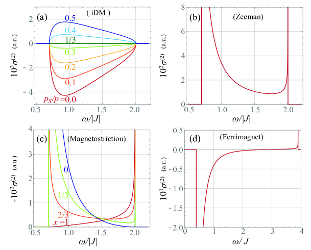
Figure 2: Nonlinear spin-current conductivity at zero temperature as a function of the frequency $\omega$ of applied linearly-polarized electromagnetic wave. Panels (a), (b) and (c) are the results of the inversion-asymmetric spin-chain model with iDM, Zeeman, and MS type spin-light couplings, respectively. Parameter $x$ denotes the ratio of uniform and staggered coupling constants: $A=x$ and $A_{s}=1-x$. Panel (d) shows the conductivity of the inversion-asymmetric antiferromagnetically ordered model. We take the 1D limit $J_{\perp}/J\to 0$ and set $g_{a}\neq g_{b}$ and $\delta\neq 0$. In all the panels, we have taken the ideal limit $1/\tau\to+0$ (Note that $1/\tau\to+0$ is not equal to $1/\tau=0$).

In the end of this section, we discuss the relaxation-time ($\tau$) dependence of the spin-current conductivity. As we mentioned, Fig. 2 depicts the conductivity at the ideal limit $1/\tau\to+0$, where quasi particles (spinons or magnons) have a sufficiently long life time. We numerically show that the conductivity is quite insensitive against the change of $\tau$. Namely, the leading term of the nonlinear conductivity is independent of the relaxation time,

$${\rm Re}[\sigma^{(2)}(0;\omega,-\omega)]\,\,\,\sim \,\,\,\text{const.}+\tau\text{-dependent\,\,\,terms}.$$ (24)

This is in sharp contrast with the usual case of injection current, in which the leading term of conductivity is proportional to $\tau$. The current satisfying the condition (24) is called shift current Kraut and von Baltz (1979); V. Belinicher and Sturman (1982); Král (2000); Sipe and Shkrebtii (2000). Therefore, the predicted spin currents are all shift current type, and it means that the photo-induced spin current is robust against impurity scattering. We emphasize that the calculated magnon shift current is the first example of a shift current carried by bosonic quasi particles to the best of our knowledge.

Finally, we explain the intuitive picture of shift current, focusing on the spin chain model (1). Due to the noncentrosymmetry, the shape of Bloch wave functions of JW fermion on conducting and valence bands are asymmetric in the unit cell, as shown in Fig. 3. If we apply THz or GHz wave with a suitable frequency, particle-hole pairs are created as in Figs. 1(c) and 3. This accompanies a “shift” of center of mass of JW fermions due to the asymmetric shape of the Bloch functions. Therefore, this photo transition makes the carrier of spin current move along a certain direction without varying the JW-fermion number, i.e., with conserving $S_{\rm tot}^{z}$. This mechanism is the origin of the word “shift”.

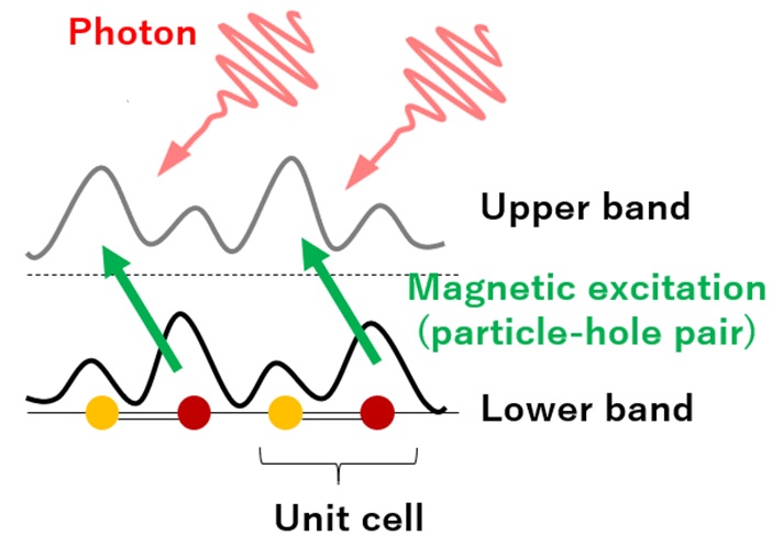
Figure 3: Intuitive real-space picture of the shift spin current in our inversion-asymmetric spin chain. Due to the inversion asymmetry, the center of mass of JW fermions in both conducting (upper) and valence (lower) bands deviates from the center of unit cell.

IV Experimental Methods, Materials, and Laser Intensity

In this section, we discuss our spin-current rectification from the experimental viewpoint. Below, we discuss the experimental ways of detecting the photo spin current, candidate materials for the rectification, and the required strength of applied THz/GHz waves.

First, we consider experimental ways Ishizuka and Sato (2019a, b) of observing the clear signature of photovoltaic spin current. The simplest way of the detection is an all-optical method described in Fig. 4(a). The setup is merely to apply a THz/GHz wave to a target magnetic material. After the continuous irradiation, a non-equilibrium steady state with a spin current is realized and a spin polarization accumulates around one and another edges, as shown in Fig. 4(a). The accumulated magnetization can be detected through inverse Faraday or Kerr effect Kirilyuk et al. (2010). Different signs of magnetizations at two edges become a clear evidence of our spin-current rectification.

The second way is based on inverse spin Hall effect Saitoh et al. (2006); Valenzuela (2006); Kimura et al. (2007) in an attached metal, and it has been often used in the field of spintronics Maekawa et al. (2012). The setup is shown in Fig. 4(b), in which we attach two heavy metals such as Pt and W to the target magnet. Due to the directionality of the photovoltaic spin current, the spin current in the magnet near one interface is injected into a metal, while the spin current near another interface is absorbed from another metal to the magnet. A part of the spin current in metals changes into an electric current via inverse spin Hall effect, and then we observe an electric voltage perpendicular to the spin-current direction. The signs of electric voltages in two attached metals give us a clear evidence of the spin-current rectification.

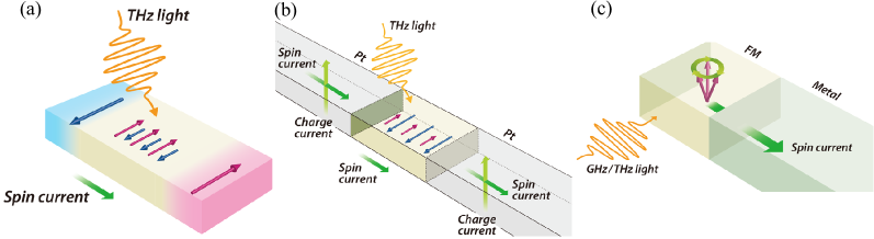
Figure 4: Possible experimental methods (a) and (b) of detecting photo-induced spin current of our proposal. As a comparison, a standard way of detecting spin current of spin pumping is depicted in the panel (c).

Next, we mention candidate materials for the photovoltaic spin current. Our theoretical analysis indicates that the photovoltaic spin current can be created in a broad class of inversion-asymmetric magnets. For instance, we can find the following inversion-asymmetric magnets: a magnetoelectric material $\rm Cr_{2}O_{3}$ McGuire et al. (1956), ferrimagnetic diamond chains Okamoto et al. (2003); Shores et al. (2005); Vilminot et al. (2005), multiferroic materials Murakawa et al. (2010); Viirok et al. (2019), and a polar ladder magnet $\rm BaFe_{2}Se_{3}$ Aoyama et al. (2019). In addition, meta magnetic materials without inversion symmetry would also be a candidate. As we showed in Sec. III.2, a large density of state in quasi-1D materials has a high potential to enhance the value of the nonlinear spin-current conductivity. Therefore, low-dimensional noncentrosymmetric magnets are expected to be a nice candidate for a large photovoltaic spin current.

Finally, we shortly discuss the required intensity of applied THz/GHz waves for the realization of the spin-current rectification. We have estimated it within a semi-quantitative level in Refs. 18; 19. According to our estimate, an AC electric fields of $10^{2-5}$ V/cm and $10^{4-6}$ V/cm are sufficient to produce an observable spin current in the asymmetric spin chains in Eq. (1) and the antiferromagnetically ordered insulators in Eq. (3), respectively. One can reach these intensities by using currently-available THz laser techniques.

V Summary and Discussions

We explained our recent theoretical proposal Ishizuka and Sato (2019a, b) of the spin-current rectification in inversion-asymmetric magnetic insulators. We show that DC spin current can be produced with a linearly polarized THz or GHz wave in inversion-asymmetric spin chains in Eq. (1) with spinon (fermionic) excitations and antiferromagnetically ordered insulators in Eq. (3) with magnon (bosonic) excitations. Our result indicates that the spin-current rectification is possible in a wide class of noncentrosymmetric magnets. We show that the photovoltaic spin current is of a shift current and stable against impurity scattering.

Thanks to the long history of magnetism, various magnetic materials have been discovered and synthesized. However, unfortunately, only a few kinds of ordered magnets such as ferro and antiferomagnets have been investigated in the field of photo-induced phenomena. Photo-driven phenomena in other various magnetic materials have a high potential to open a new field of magneto-optics and photonics.

Finally, we compare our proposal of the spin-current rectification with the well-established spin pumping effect Kajiwara et al. (2010); Heinrich et al. (2011). The latter effect is a representative of producing a DC spin current with external electromagnetic waves.

A typical setup of spin pumping is described in Fig. 4(c) and is basically the same as a standard magnetic resonance in magnets, as shown in Fig. 5(a). If we apply GHz or THz wave with the resonant frequency to an ordered magnet, the magnetic resonance occurs and many magnons are created. This is an angular momentum transfer from photons to magnons, namely, the value of $S_{\rm tot}^{z}$ is changed. Created magnons diffusively spread in all directions as in Fig. 5(a), and it means the production of a diffusive spin current. For the detection of the diffusive spin current, the attachment of a heavy metal has been often used like our proposed method in Fig. 4(b). However, the spin-pumped spin current is always injected into the metal irrespective of the direction of the interface between the magnet and the metal.

On the other hand, as we discussed in the previous section, the photovoltaic spin current propagates along a certain direction, which determines from the inversion-symmetry breaking of the crystal, as shown in Fig. 5(b). This directionality nature is essentially different from diffusion dynamics of spin pumping. Therefore, the attachment of a heavy metal is not always necessary to detect photo-induced spin current, in principle. In addition, as we already mentioned, the photo spin current does not accompany the change of $S_{\rm tot}^{z}$ and is shift current type. Moreover, the AC-field polarization dependence would be useful to distinguish spin current rectification and spin pumping.

From these arguments, one sees that the predicted spin current rectification is essentially different from the established spin pumping phenomenon. There is a possibility that spin currents already observed in spin pumping experiments include the photovoltaic spin current.

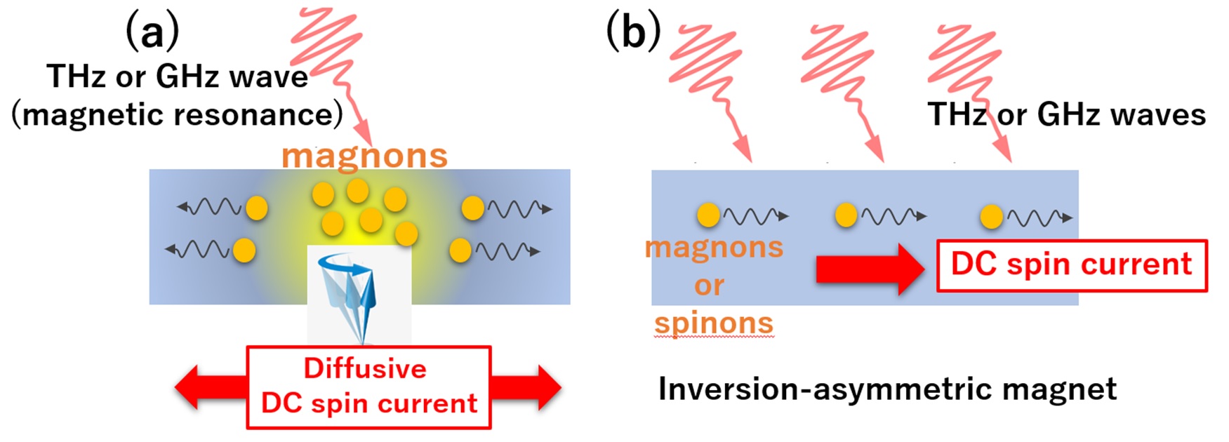
Figure 5: Schematic setups of (a) spin pumping and (b) spin-current rectification (our proposal). The setup of spin pumping is basically the same as the standard magnetic resonance. Due to the GHz or THz wave-driven magnetic resonance, a plenty of magnons are created and then diffusively spread. On the other hand, in the case of the rectification (b), a spin current is created by photo-induced magnetic excitations and its flow direction is uniquely determined by the inversion asymmetry of the crystal.

References

- Sturman and Fridkin (1992) B. I. Sturman and V. M. Fridkin, The Photovoltaic and Photorefractive Effects in Noncentrosymmetric Materials (Gordon and Breach, Philadelphia, 1992).
- Kohli et al. (2011) K. K. Kohli, J. Mertens, M. Bieler, and S. Chatterjee, J. Opt. Soc. Am. B 28, 470 (2011).
- Cote et al. (2002) D. Cote, N. Laman, and H. M. van Driel, Applied Physics Letters 80, 905 (2002).
- Sotome et al. (2019) M. Sotome, M. Nakamura, J. Fujioka, M. Ogino, Y. Kaneko, T. Morimoto, Y. Zhang, M. Kawasaki, N. Nagaosa, Y. Tokura, et al., Proceedings of the National Academy of Sciences 116, 1929 (2019).
- Koch et al. (1976) W. T. H. Koch, R. Munser, W. Ruppel, and P. Wurfel, Ferroelectrics 13, 305 (1976).
- Dalba et al. (1995) G. Dalba, Y. Soldo, F. Rocca, V. M. Fridkin, and P. Sainctavit, Phys. Rev. Lett. 74, 988 (1995).
- Nakamura et al. (2017) M. Nakamura, S. Horiuchi, F. Kagawa, N. Ogawa, T. Kurumaji, Y. Tokura, and M. Kawasaki, Nature Communications 8, 281 (2017).
- Kraut and von Baltz (1979) W. Kraut and R. von Baltz, Phys. Rev. B 19, 1548 (1979).
- V. Belinicher and Sturman (1982) E. L. I. V. Belinicher and B. Sturman, Zh. Eksp. Teor. Fiz. 83, 649 (1982).
- Král (2000) P. Král, Journal of Physics: Condensed Matter 12, 4851 (2000).
- Sipe and Shkrebtii (2000) J. E. Sipe and A. I. Shkrebtii, Phys. Rev. B 61, 5337 (2000).
- Young and Rappe (2012) S. M. Young and A. M. Rappe, Phys. Rev. Lett. 109, 116601 (2012).
- Morimoto and Nagaosa (2016) T. Morimoto and N. Nagaosa, Science Advances 2, e1501524 (2016).
- Cook et al. (2017) B. Cook, Ashley M.and M. Fregoso, F. de Juan, S. Coh, and J. E. Moore, Nature Communications 8, 14176 (2017).
- Ishizuka and Nagaosa (2017) H. Ishizuka and N. Nagaosa, New Journal of Physics 19, 033015 (2017).
- Kirilyuk et al. (2010) A. Kirilyuk, A. V. Kimel, and T. Rasing, Rev. Mod. Phys. 82, 2731 (2010).
- Němec and Kimel (2018) M. K. T. Němec, P. Fiebig and A. V. Kimel, Nature Physics 14, 229 (2018).
- Ishizuka and Sato (2019a) H. Ishizuka and M. Sato, Phys. Rev. Lett. 122, 197702 (2019a).
- Ishizuka and Sato (2019b) H. Ishizuka and M. Sato, Phys. Rev. B 100, 224411 (2019b).
- Maekawa et al. (2012) S. Maekawa, S. O. Valenzuela, E. Saitoh, and T. Kimura, eds., Spin Current (Oxford University Press, Oxford, U.K., 2012).
- Hirori et al. (2011) H. Hirori, A. Doi, F. Blanchard, and K. Tanaka, Applied Physics Letters 98, 091106 (2011).
- Sato et al. (2013) M. Sato, T. Higuchi, N. Kanda, K. Konishi, K. Yoshioka, T. Suzuki, K. Misawa, and M. Kuwata-Gonokami, Nature Photonics 7, 724 (2013).
- Liu et al. (2017) B. Liu, H. Bromberger, A. Cartella, T. Gebert, M. Först, and A. Cavalleri, Opt. Lett. 42, 129 (2017).
- Mukai et al. (2016) Y. Mukai, H. Hirori, T. Yamamoto, H. Kageyama, and K. Tanaka, New Journal of Physics 18, 013045 (2016).
- Baierl et al. (2016) S. Baierl, J. H. Mentink, M. Hohenleutner, L. Braun, T.-M. Do, C. Lange, A. Sell, M. Fiebig, G. Woltersdorf, T. Kampfrath, et al., Phys. Rev. Lett. 117, 197201 (2016).
- Kubacka et al. (2014) T. Kubacka, J. A. Johnson, M. C. Hoffmann, C. Vicario, S. de Jong, P. Beaud, S. Grübel, S.-W. Huang, L. Huber, L. Patthey, et al., Science 343, 1333 (2014).
- Lu et al. (2017) J. Lu, X. Li, H. Y. Hwang, B. K. Ofori-Okai, T. Kurihara, T. Suemoto, and K. A. Nelson, Phys. Rev. Lett. 118, 207204 (2017).
- Takayoshi et al. (2014a) S. Takayoshi, H. Aoki, and T. Oka, Phys. Rev. B 90, 085150 (2014a).
- Takayoshi et al. (2014b) S. Takayoshi, M. Sato, and T. Oka, Phys. Rev. B 90, 214413 (2014b).
- Sato et al. (2016) M. Sato, S. Takayoshi, and T. Oka, Phys. Rev. Lett. 117, 147202 (2016).
- Fujita and Sato (2017) H. Fujita and M. Sato, Phys. Rev. B 96, 060407 (2017).
- Ikeda and Sato (2019) T. N. Ikeda and M. Sato, Phys. Rev. B 100, 214424 (2019).
- Sato and Morisaku (2020) M. Sato and Y. Morisaku, Phys. Rev. B 102, 060401 (2020).
- Giamarchi (2003) T. Giamarchi, Quantum Physics in One Dimension (Oxford University Press, New York, 2003).
- A. O. Gogolin and Tsvelik (2004) A. A. N. A. O. Gogolin and A. M. Tsvelik, Bosonization and Strongly Correlated Systems (Cambridge University Press, Cambridge, England, 2004).
- Tsvelik (2007) A. M. Tsvelik, Quantum Field Theory in Condensed Matter Physics (Cambridge University Press, Cambridge, England, 2007).
- Dender et al. (1997) D. C. Dender, P. R. Hammar, D. H. Reich, C. Broholm, and G. Aeppli, Phys. Rev. Lett. 79, 1750 (1997).
- Oshikawa et al. (1999) M. Oshikawa, K. Ueda, H. Aoki, A. Ochiai, and M. Kohgi, Journal of the Physical Society of Japan 68, 3181 (1999).
- Feyerherm et al. (2000) R. Feyerherm, S. Abens, D. Günther, T. Ishida, M. Meißner, M. Meschke, T. Nogami, and M. Steiner, Journal of Physics: Condensed Matter 12, 8495 (2000).
- Umegaki et al. (2009) I. Umegaki, H. Tanaka, T. Ono, H. Uekusa, and H. Nojiri, Phys. Rev. B 79, 184401 (2009).
- Affleck and Oshikawa (1999) I. Affleck and M. Oshikawa, Phys. Rev. B 60, 1038 (1999).
- Scalapino et al. (1975) D. J. Scalapino, Y. Imry, and P. Pincus, Phys. Rev. B 11, 2042 (1975).
- Schulz (1996) H. J. Schulz, Phys. Rev. Lett. 77, 2790 (1996).
- Sato and Oshikawa (2004) M. Sato and M. Oshikawa, Phys. Rev. B 69, 054406 (2004).
- Okunishi and Suzuki (2007) K. Okunishi and T. Suzuki, Phys. Rev. B 76, 224411 (2007).
- Ishimura and Shiba (1980) N. Ishimura and H. Shiba, Progress of Theoretical Physics 63, 743 (1980), ISSN 0033-068X.
- Coldea et al. (2010) R. Coldea, D. A. Tennant, E. M. Wheeler, E. Wawrzynska, D. Prabhakaran, M. Telling, K. Habicht, P. Smeibidl, and K. Kiefer, Science 327, 177 (2010).
- Yoshida (1996) K. Yoshida, Theory of Magnetism (Springer, 1996).
- Mattis (2006) D. C. Mattis, The Theory of Magnetism Made Simple (World Scientific Pub Co Inc, 2006).
- Tokura et al. (2014) Y. Tokura, S. Seki, and N. Nagaosa, Reports on Progress in Physics 77, 076501 (2014).
- Katsura et al. (2005) H. Katsura, N. Nagaosa, and A. V. Balatsky, Phys. Rev. Lett. 95, 057205 (2005).
- Saitoh et al. (2006) E. Saitoh, M. Ueda, H. Miyajima, and G. Tatara, Applied Physics Letters 88, 182509 (2006).
- Valenzuela (2006) M. Valenzuela, S. O.and Tinkham, Nature 442, 176 (2006).
- Kimura et al. (2007) T. Kimura, Y. Otani, T. Sato, S. Takahashi, and S. Maekawa, Phys. Rev. Lett. 98, 156601 (2007).
- McGuire et al. (1956) T. R. McGuire, E. J. Scott, and F. H. Grannis, Phys. Rev. 102, 1000 (1956).
- Okamoto et al. (2003) K. Okamoto, T. Tonegawa, and M. Kaburagi, Journal of Physics: Condensed Matter 15, 5979 (2003).
- Shores et al. (2005) M. P. Shores, B. M. Bartlett, and D. G. Nocera, Journal of the American Chemical Society 127, 17986 (2005).
- Vilminot et al. (2005) S. Vilminot, G. André, M. Richard-Plouet, F. Bourée-Vigneron, and M. Kurmoo, Inorganic Chemistry 45, 10938 (2005).
- Murakawa et al. (2010) H. Murakawa, Y. Onose, S. Miyahara, N. Furukawa, and Y. Tokura, Phys. Rev. Lett. 105, 137202 (2010).
- Viirok et al. (2019) J. Viirok, U. Nagel, T. Rõ om, D. G. Farkas, P. Balla, D. Szaller, V. Kocsis, Y. Tokunaga, Y. Taguchi, Y. Tokura, et al., Phys. Rev. B 99, 014410 (2019).
- Aoyama et al. (2019) T. Aoyama, S. Imaizumi, T. Togashi, Y. Sato, K. Hashizume, Y. Nambu, Y. Hirata, M. Matsubara, and K. Ohgushi, Phys. Rev. B 99, 241109 (2019).
- Kajiwara et al. (2010) Y. Kajiwara, K. Harii, S. Takahashi, J. Ohe, K. Uchida, M. Mizuguchi, H. Umezawa, H. Kawai, K. Ando, K. Takanashi, et al., Nature 464, 262 (2010).
- Heinrich et al. (2011) B. Heinrich, C. Burrowes, E. Montoya, B. Kardasz, E. Girt, Y.-Y. Song, Y. Sun, and M. Wu, Phys. Rev. Lett. 107, 066604 (2011).