Label-Aware Neural Tangent Kernel:
Toward Better Generalization and Local Elasticity

Abstract

As a popular approach to modeling the dynamics of training overparametrized neural networks (NNs), the neural tangent kernels (NTK) are known to fall behind real-world NNs in generalization ability. This performance gap is in part due to the label agnostic nature of the NTK, which renders the resulting kernel not as locally elastic as NNs (He & Su, 2020). In this paper, we introduce a novel approach from the perspective of label-awareness to reduce this gap for the NTK. Specifically, we propose two label-aware kernels that are each a superimposition of a label-agnostic part and a hierarchy of label-aware parts with increasing complexity of label dependence, using the Hoeffding decomposition. Through both theoretical and empirical evidence, we show that the models trained with the proposed kernels better simulate NNs in terms of generalization ability and local elasticity.

1 Introduction

The last decade has witnessed the huge success of deep neural networks (NNs) in various machine learning tasks (LeCun et al., 2015). Contrary to its empirical success, however, the theoretical understanding of real-world NNs is still far from complete, hindering its applicability to many domains where interpretability is of great importance, such as autonomous driving and biological research (Doshi-Velez & Kim, 2017).

More recently, a venerable line of work relates overparametrized NNs to kernel regression from the perspective of their training dynamics, providing positive evidence towards understanding the optimization and generalization of NNs (Jacot et al., 2018; Chizat & Bach, 2018; Cao & Gu, 2019; Lee et al., 2019; Arora et al., 2019a; Chizat et al., 2019; Du et al., 2019; Li et al., 2019; Zou et al., 2020). To briefly introduce this approach, let $\bm{x}_{i},y_{i}$ be the feature and label, respectively, of the $i$th data point, and consider the problem of minimizing the squared loss $\frac{1}{n}\sum_{i=1}^{n}(y_{i}-f(\bm{x}_{i},{\bm{w}}))^{2}$ using gradient descent, where $f(\bm{x},{\bm{w}})$ denotes the prediction of NNs and $\bm{w}$ are the weights. Starting from an random initialization, researchers demonstrate that the evolution of NNs in terms of predictions can be well captured by the following kernel gradient descent

$$\frac{d}{dt}f(\bm{x},{\bm{w}}_{t})=-\frac{1}{n}\sum_{i=1}^{n}{K(\bm{x},\bm{x}_{i})}\bigl{(}f(\bm{x}_{i},{\bm{w}}_{t})-y_{i}\bigr{)}$$ (1)

in the infinite width limit, where ${\bm{w}}_{t}$ is the weights at time $t$. Above, $K(\cdot,\cdot)$, referred to as neural tangent kernel (NTK), is time-independent and associated with the architecture of the NNs. As a profound implication, an infinitely wide NNs is “equivalent” to kernel regression with a deterministic kernel in the training process.

Despite its immense popularity, many questions still remain unanswered concerning the NTK approach, with the most crucial one, perhaps, being the non-negligible performance gap between a kernel regression using the NTK and a real-world NNs. Indeed, according to an experiment done by Arora et al. (2019a), on the CIFAR-10 dataset (Krizhevsky, 2009), a vanilla 21-layer CNN can achieve $75.57\%$ accuracy, whereas the corresponding convolutional NTK (CNTK) can only attain $64.09\%$ accuracy. This significant performance gap is widely recognized to be attributed to the finiteness of widths in real-world NNs. This perspective has been investigated in many papers (Hanin & Nica, 2019; Huang & Yau, 2019; Bai & Lee, 2019; Bai et al., 2020), where various forms of “finite-width corrections” have been proposed. However, the computation of these corrections all involve incremental training. This fact is in sharp contrast to kernel methods, whose computation is “one-shot” via solving a simple linear system.

In this paper, we develop a new approach toward closing the gap by recognizing a recently introduced phenomenon termed local elasticity in training neural networks (He & Su, 2020). Roughly speaking, neural networks are observed to be locally elastic in the sense that if the prediction at a feature vector $\bm{x}$ is not significantly perturbed, after the classifier is updated via stochastic gradient descent at a (labeled) feature vector $\bm{x}$ that is dissimilar to $\bm{x}^{\prime}$ in a certain sense. This phenomenon implies that the interaction between two examples is heavily contingent upon whether their labels are the same or not. Unfortunately, the NTK construction is clearly independent of the labels, thereby being label-agnostic, meaning that it is independent of the labels $y$ in the training data. This ignorance of the label information can cause huge problems in practice, especially when the semantic meanings of the features crucially depends on the label system.

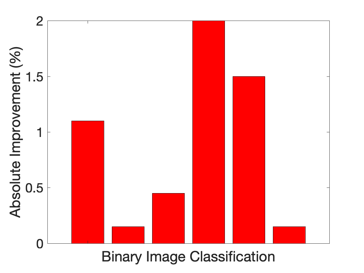
(a) NTK: init vs trained

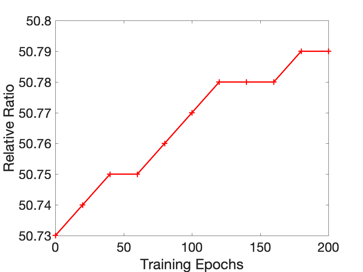
(b) Local elasticity: cat vs dog

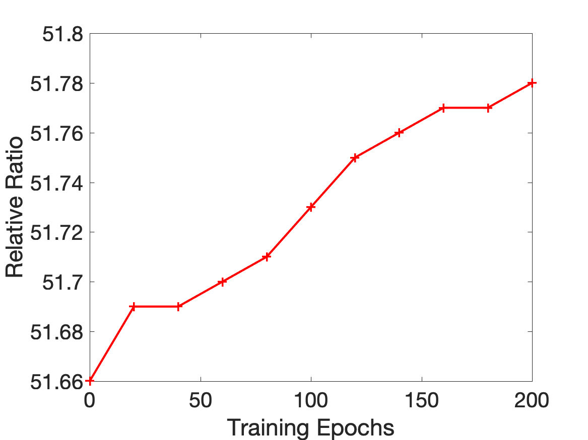
(c) Local elasticity: chair vs bench

Figure 1: The impact of labels on a 2-layer NN in the aspect of generalization ability and local elasticity. Fig. (a) displays the absolute improvement in six binary classification tasks by using ${K}^{(2)}_{t}$ instead of ${K}^{(2)}_{0}$, indicating that NNs learn better feature representations with the help of labels along the training process (see Sec. 3.2 for more details). Fig. (b) and (c) show that in two label systems (cat v.s. dog and bench v.s. chair), the strength of local elasticity (measured by the relative ratio defined in Eq. (9)) both increases with training, but in different patterns, indicating that the labels play an important role in the local elasticity of NNs (See Appx. D.1 for more details).

To shed light on the vital importance of the label information, consider a collection of natural images, where in each image, there are two objects: one object is either a cat or dog, and another is either a bench or chair. Take an image $\bm{x}$ that contains dog+chair, and another $\bm{x}^{\prime}$ that contains dog+bench. Then for NTK to work well on both label systems, we would need ${\mathbb{E}}_{\textnormal{init}}K(\bm{x},\bm{x}^{\prime})\approx 1$ if the task is dog v.s. cat, and ${\mathbb{E}}_{\textnormal{init}}K(\bm{x},\bm{x}^{\prime})\approx-1$ if the task is bench v.s. chair, a fundamental contradiction that cannot be resolved by the label-agnostic NTK (see also Claim 1.1). In contrast, NNs can do equally well in both label systems, a favorable property which can be termed adaptivity to label systems. To understand what is responsible for this desired adaptivity, note that (1) suggests that NNs can be thought of as a time-varying kernel ${K}^{(2)}_{t}$. This “dynamic” kernel differs from the NTK in that it is label-aware, because it depends on the trained parameter ${\bm{w}}_{t}$ which further depends on $y$. As shown in Fig. 1, such an awareness in labels play an import role in the generalization ability and local elasticity of NNs.

Thus, in the search of “NN-simulating” kernels, it suffices to limit our focus on the class of label-aware kernels. In this paper, we propose two label-aware NTKs (LANTKs). The first one is based on a notion of higher-order regression, which extracts higher-order information from the labels by estimating whether two examples are from the same class or not. The second one is based on approximately solving neural tangent hierarchy (NTH), an infinite hierarchy of ordinary different equations that give a precise description of the training dynamics (1) (Huang & Yau, 2019), and we show this kernel approximates ${K}^{(2)}_{t}$ strictly better than ${\mathbb{E}}_{\textnormal{init}}{K}^{(2)}_{0}$ does (Theorem 2.1).

Although the two LANTKs stems from very different intuitions, their analytical formulas are perhaps surprisingly similar: they are both quadratic functions of the label vector $y$. This brings a natural question: is there any intrinsic relationship between the two? And more generally, what does a generic label-aware kernel, $K(\bm{x},\bm{x}^{\prime},S)$, which may have arbitrary dependence structure on the training data $S=\{(\bm{x}_{i},y_{i}):i\in[n]\}$, look like? Using Hoeffding Decomposition (Hoeffding et al., 1948), we are able to obtain a structural lemma (Lemma 2.2), which asserts that any label-aware kernel can be decomposed into the superimposition of a label-agnostic part and a hierarchy of label-aware parts with increasing complexity of label dependence. And the two LANTKs we developed can, in a certain sense, be regarded as the truncated versions of this hierarchy.

We conduct comprehensive experiments to confirm that our proposed LANTKs can indeed better simulate the quantitative and qualitative behaviors of NNs compared to their label-agnostic counterpart. On the one hand, they generalize better: the two LANTKs achieve a $1.04\%$ and $1.94\%$ absolute improvement in test accuracy ($7.4\%$ and $4.1\%$ relative error reductions) in binary and multi-class classification tasks on CIFAR-10, respectively. On the other hand, they are more “locally elastic”: the relative ratio of the kernelized similarity between intra-class examples and inter-class examples increases, a typical trend observed along the training trajectory of NNs.

1.1 Related Work

Kernels and NNs. Starting from Neal (1996), a line of work considers infinitely wide NNs whose parameters are chosen randomly and only the last layer is optimized (Williams, 1997; Le Roux & Bengio, 2007; Hazan & Jaakkola, 2015; Lee et al., 2017; Matthews et al., 2018; Novak et al., 2018; Garriga-Alonso et al., 2018; Yang, 2019). When the loss is the least squares loss, this gives rise to a class of interesting kernels different from the NTK. On the other hand, if all layers are trained by gradient descent, infinitely wide NNs give rise to the NTK (Jacot et al., 2018; Chizat & Bach, 2018; Lee et al., 2019; Arora et al., 2019a; Chizat et al., 2019; Du et al., 2019; Li et al., 2019), and the NTK also appears implicitly in many works when studying the optimization trajectories of NN training (Li & Liang, 2018; Allen-Zhu et al., 2018; Du et al., 2018; Ji & Telgarsky, 2019; Chen et al., 2019).

Limitations of the NTK and corrections. Arora et al. (2019b) demonstrates that in many small datasets, models trained by the NTK can outperform its corresponding NN. But for moderately large scale tasks and for practical architectures, the performance gap between the two is empirically observed in many places and further confirmed by a series of theoretical works (Chizat et al., 2019; Ghorbani et al., 2019b; Yehudai & Shamir, 2019; Bietti & Mairal, 2019; Ghorbani et al., 2019a; Wei et al., 2019; Allen-Zhu & Li, 2019). This observation motivates various attempts to mitigate the gap, such as incorporating pooling layers and data augmentation into the NTK (Li et al., 2019), deriving higher-order expansions around the initialization (Bai & Lee, 2019; Bai et al., 2020), doing finite-width correction (Hanin & Nica, 2019), injecting noise to gradient descent (Chen et al., 2020), and most related to our work, the NTH (Huang & Yau, 2019).

Label-aware kernels. The idea of incorporating label information into the kernel is not entirely new. For example, Cristianini et al. (2002) proposes an alignment measure between two kernels, and argues that aligning a label-agnostic kernel to the “optimal kernel” $yy^{\top}$ can lead to favorable generalization guarantees. This idea is extensively exploited in literature on kernel learning (see, e.g., Lanckriet et al. 2004; Cortes et al. 2012; Gönen & Alpaydin 2011). In another related direction, Tishby et al. (2000) proposes the information bottleneck principle, which roughly says that an optimal feature map should simultaneously minimize its mutual information (MI) with the feature distribution and maximize its MI with the label distribution, thus incorporating the label information (see also Tishby & Zaslavsky 2015 in the context of deep learning). We refer the readers to Appx. C for a detailed discussion of the connections and differences of our proposals to these two lines of research.

1.2 Preliminaries

We focus on binary classification tasks for ease of exposition, but our results can be easily extend to multi-class classification tasks. Suppose we have i.i.d. data $S=\{(\bm{x}_{i},y_{i}):i\in[n]\}\subseteq\mathbb{R}^{d}\times\{\pm 1\}$. Let ${\mathbf{X}}\in\mathbb{R}^{n\times d}$ be the feature matrix and let $y\in\{\pm 1\}^{n}$ be the vector of labels. Let ${\bm{w}}=\{({\mathbf{W}}^{(\ell)},{\mathbf{b}}^{(\ell)})\in{\mathbb{R}}^{p_{\ell}\times q_{\ell}}\times{\mathbb{R}}^{q_{\ell}}:\ell\in[L]\}$ be the collection of weights and biases at each layer. A neural network function is recursively defined as $\bm{x}^{{}(0)}=\bm{x},\bm{x}^{{}(\ell)}=\frac{1}{\sqrt{q_{\ell}}}\sigma({\mathbf{W}}^{{}(\ell)}\bm{x}^{{}(\ell-1)}+{\mathbf{b}}^{{}(\ell)})$ and $f(\bm{x},{\bm{w}})=\bm{x}^{{}(L)}$, where $\sigma$ is the activation function which applies element-wise to matrices. Note that $q_{1}=d$ and $p_{L}=1$.

Consider training NNs with least squares loss: $L({\bm{w}})=\frac{1}{2n}\sum_{i=1}^{n}\bigl{(}f(\bm{x}_{i},{\bm{w}})-y_{i}\bigr{)}^{2}$. The gradient flow dynamics (i.e., gradient descent with infinitesimal step sizes) is given by $\dot{{\bm{w}}_{t}}=-\frac{\partial}{\partial{\bm{w}}}L({\bm{w}}_{t}),$ where we use the dot notation to denote the derivative w.r.t. time, and ${\bm{w}}_{t}$ is the parameter value at time $t$. The dynamics w.r.t. $f$ is given by a kernel gradient descent (1), where the corresponding second-order kernel is given by ${K}^{(2)}_{t}(\bm{x},\bm{x}^{\prime})=\langle\frac{\partial}{\partial{\bm{w}}}f(\bm{x},{\bm{w}}_{t}),\frac{\partial}{\partial{\bm{w}}}f(\bm{x}^{\prime},{\bm{w}}_{t})\rangle$. With sufficient over-parameterization, one can show that ${K}^{(2)}_{t}\approx{K}^{(2)}_{0}$, and with Gaussian initialization, one can show that ${K}^{(2)}_{0}$ concentrates around ${\mathbb{E}}_{\textnormal{init}}{K}^{(2)}_{0}$, where ${\mathbb{E}}_{\textnormal{init}}$ is the expectation operator w.r.t. the random initialization. Hence, ${K}^{(2)}_{t}$ can be approximated by the deterministic kernel ${\mathbb{E}}_{\textnormal{init}}{K}^{(2)}_{0}$, the NTK.

We have heuristically argued in Section 1 that the label-agnostic property of NTK can cause problems when the semantic meaning of the features is highly dependent on the label system. To further illustrate this point, in Appx. A.1, we construct a simple example that validates the following claim:

Claim 1.1 (Curse of Label-Agnosticism).

If a kernel $K$ is label-agnostic and it works well on one label system, then there exists a natural relabeling, which gives another label system on which $K$ performs arbitrarily bad. In other words, $K$ is not adaptive to different label systems.

We make two remarks. The above claim applies to any label-agnostic kernels, and the NTK is only a specific example. Moreover, the above claim only applies to the generalization error. A label-agnostic kernel can always achieve zero training error, as long as the corresponding kernel matrix is invertible.

2 Construction of Label-Aware NTKs

We now propose two ways to incorporate label awareness into NTKs. In Section 2.3, we give a unified interpretation of the two approaches using the Hoeffding decomposition.

2.1 Label-Aware NTK via Higher-Order Regression

We shall all agree that a “good” feature map should map the feature vector $\bm{x}$ to $\phi(\bm{x})$ s.t. a simple linear fit in the $\phi(\cdot)$-space can give satisfactory performance. In this sense, the “optimal” feature map is obviously its corresponding label: $\phi(\bm{x}):=\textnormal{label of }\bm{x}$. Hence, for $\alpha,\beta\in[n]$, the corresponding “optimal” kernel is given by $K^{\star}(\bm{x}_{\alpha},\bm{x}_{\beta})=y_{\alpha}y_{\beta}.$ This motivates us to consider interpolating the NTK with the optimal kernel: ${\mathbb{E}}_{\textnormal{init}}K^{(2)}_{0}(\bm{x}_{\alpha},\bm{x}_{\beta})+\lambda K^{\star}(\bm{x}_{\alpha},\bm{x}_{\beta})={\mathbb{E}}_{\textnormal{init}}K^{(2)}_{0}(\bm{x}_{\alpha},\bm{x}_{\beta})+\lambda y_{\alpha}y_{\beta},$ where $\lambda\geq 0$ controls the strength of the label information. However, this interpolated kernel cannot be calculated on the test data. A natural solution is to estimate $y_{\alpha}y_{\beta}$. Thus, we propose to use the following kernel, which we term as LANTK-HR:

$$K^{(\textnormal{HR})}(\bm{x},\bm{x}^{\prime}):={\mathbb{E}}_{\textnormal{init}}K^{(2)}_{0}(\bm{x},\bm{x}^{\prime})+\lambda{\mathcal{Z}}(\bm{x},\bm{x}^{\prime},S),$$ (2)

where ${\mathcal{Z}}(\bm{x},\bm{x}^{\prime},S)$ is an estimator of $(\textnormal{label of }\bm{x})\times(\textnormal{label of }\bm{x}^{\prime})$ — a quantity indicating whether both features belong to the same class or not — using the dataset $S$.

A natural way to obtain ${\mathcal{Z}}$ is to form a new pairwise dataset $\bigl{\{}\bigl{(}(\bm{x}_{i},\bm{x}_{j}),y_{i}y_{j}\bigr{)}:i,j\in[n]\bigr{\}}$, where we think of $y_{i}y_{j}$ as the label of the augmented feature vector $(\bm{x}_{i},\bm{x}_{j})$. If we use a linear regression model, then we would have ${\mathcal{Z}}(\bm{x},\bm{x}^{\prime},S)=y^{\top}{\mathbf{M}}(\bm{x},\bm{x}^{\prime},{\mathbf{X}})y$ for some matrix ${\mathbf{M}}\in\mathbb{R}^{n\times n}$ depending on the two feature vectors $\bm{x},\bm{x}^{\prime}$ as well as the feature matrix ${\mathbf{X}}$, hence the name “higher-order regression”.

What requirement we do need to impose on the estimator ${\mathcal{Z}}$? Heuristically, the inclusion of ${\mathcal{Z}}$ is only helpful when additional information in the training data is “extracted” apart from the one extracted by the label-agnostic part. We refer the readers to Sec. 3.1 and Appx. D.3 for more details on the choice of ${\mathcal{Z}}$.

2.2 Label-Aware NTK via Approximately Solving NTH

As we have discussed in Section 1, different from the label-agnostic NTK ${\mathbb{E}}_{\textnormal{init}}{K}^{(2)}_{0}$, the time-dependent kernel ${K}^{(2)}_{t}$ is indeed label-aware. This suggests that in real-world neural network training, ${K}^{(2)}_{t}$ must drift away from ${K}^{(2)}_{0}$ by a non-negligible amount. Indeed, Huang & Yau (2019) prove that the second order kernel ${K}^{(2)}_{t}$ evolves according to the following infinite hierarchy of ordinary differential equations (that is, the NTH):

$$\dot{K}^{(r)}_{t}(\bm{x}_{\alpha_{1}},\cdots,\bm{x}_{\alpha_{r}}) =-\frac{1}{n}\sum_{i\in[n]}K^{(r+1)}_{t}(\bm{x}_{\alpha_{1}},\cdots,\bm{x}_{\alpha_{r}},\bm{x}_{i})(f_{t}(\bm{x}_{i})-y_{i}),\ \ \ r\geq 2,$$ (3)

which, along with (1), gives a precise description of the training dynamics of NNs. Here, $K_{t}^{(r)}$ is an $r$-th order kernel which takes $r$ feature vectors as the input.

Our second construction of LANTK is to obtain a finer approximation of ${K}^{(2)}_{t}$. Let ${\mathbf{f}}_{t}$ be the vector of $f_{t}(\bm{x}_{i})$’s. Using (3), we can re-write ${K}^{(2)}_{t}(\bm{x},\bm{x}^{\prime})$ as ${K}^{(2)}_{0}(\bm{x},\bm{x}^{\prime})-\frac{1}{n}\int_{0}^{t}\langle{K}^{(3)}_{0}(\bm{x},\bm{x}^{\prime},\cdot),{\mathbf{f}}_{u}-y\rangle du+\frac{1}{n^{2}}\int_{0}^{t}\int_{0}^{u}({\mathbf{f}}_{u}-y)^{\top}{K}^{(4)}_{v}(\bm{x},\bm{x}^{\prime},\cdot,\cdot)({\mathbf{f}}_{v}-y)dvdu,$ where ${K}^{(3)}_{t}(\bm{x},\bm{x}^{\prime},\cdot)$ is an $n$-dimensional vector whose $i$-th coordinate is ${K}^{(3)}_{t}(\bm{x},\bm{x}^{\prime},\bm{x}_{i})$, and ${K}^{(4)}_{t}(\bm{x},\bm{x}^{\prime},\cdot,\cdot)$ is an $n\times n$ matrix, whose $(i,j)$-th entry is ${K}^{(4)}_{t}(\bm{x},\bm{x}^{\prime},\bm{x}_{i},\bm{x}_{j})$. Now, let ${{\mathbf{K}}}^{(2)}_{0}\in\mathbb{R}^{n\times n}$ be the kernel matrix corresponding to ${K}^{(2)}_{0}$ computed on the training data. The kernel gradient descent using ${{\mathbf{K}}}^{(2)}_{0}$ is characterized by $\dot{{\mathbf{h}}}_{t}=-\frac{1}{n}{{\mathbf{K}}}^{(2)}_{0}({\mathbf{h}}_{t}-y)$ with the initial value condition ${\mathbf{h}}_{0}={\mathbf{f}}_{0}$, whose solution is given by ${\mathbf{h}}_{t}=({\mathbf{I}}_{n}-e^{-t{{\mathbf{K}}}^{(2)}_{0}/n})y+{\mathbf{h}}_{0}.$ For a wide enough network, we expect ${\mathbf{h}}_{t}\approx{\mathbf{f}}_{t}$, at least when $t$ is not too large. On the other hand, it has been shown in Huang & Yau (2019) that ${K}^{(4)}_{t}$ varies at a rate of $\tilde{O}(1/m^{2})$, where $\tilde{O}$ hides the poly-log factors and $m$ is the (minimum) width of the network. Hence, it is reasonable to approximate ${K}^{(4)}_{t}$ by ${K}^{(4)}_{0}$. This motivates us to write

$${K}^{(2)}_{t}(\bm{x},\bm{x}^{\prime}) =\hat{K}^{(2)}_{t}(\bm{x},\bm{x}^{\prime})+{\mathcal{E}}$$ (4)

where ${\mathcal{E}}$ is a small error term and $\hat{K}^{(2)}_{t}(\bm{x},\bm{x}^{\prime})={K}^{(2)}_{0}(\bm{x},\bm{x}^{\prime})-\frac{1}{n}\int_{0}^{t}\langle{K}^{(3)}_{0}(\bm{x},\bm{x}^{\prime},\cdot),{\mathbf{h}}_{u}-y\rangle du+\frac{1}{n^{2}}\int_{0}^{t}\int_{0}^{u}({\mathbf{h}}_{u}-y)^{\top}{K}^{(4)}_{0}(\bm{x},\bm{x}^{\prime},\cdot,\cdot)({\mathbf{h}}_{v}-y)dvdu$.

In Appx. A.2, we show that ${\hat{K}}^{(2)}_{t}$ can be evaluated analytically, and the analytical expression is of the form ${K}^{(2)}_{0}+{\mathbf{a}}^{\top}y+y^{\top}{\mathbf{B}}y$ for some vector ${\mathbf{a}}$ and matrix ${\mathbf{B}}$ (see Proposition A.2 for the exact formula). Moreover, the approximation (4) can be justified formally under mild regularity conditions:

Theorem 2.1 (Validity of ${\hat{K}}^{(2)}_{t}$).

Consider a neural network with ${\mathbf{b}}^{(\ell)}=0\ \forall\ell$ and $p_{\ell}=q_{\ell}=m$ except for $q_{1}=d,p_{L}=1$. We train this net using gradient flow with the least squares loss and Gaussian initialization. Under Assumption A in Appendix A.4, with probability at least $1-e^{-Cm}$ w.r.t. the initialization, the error of the approximation (4) at time $t$ satisfies

$$|{\mathcal{E}}|\lesssim\frac{(\log m)^{c}}{m^{2}}\times\bigg{[}t^{2}(t^{2}\lor 1)\bigg{(}1+\frac{t^{2}}{m}\bigg{)}\bigg{(}t\land\frac{n}{\lambda}\bigg{)}+t^{3}(1\lor t)\bigg{]}\textnormal{ provided }t\lesssim\bigg{(}{\frac{\sqrt{\lambda m/n}}{(\log m)^{c^{\prime}}}}\land\frac{m^{1/3}}{(\log m)^{c^{\prime\prime}}}\bigg{)},$$

where $C,c,c^{\prime},c^{\prime\prime}$ are some absolute constants and $\lambda$ is a quantity defined in Asumption A. On the other hand, on the same high probability event, the three terms in $\hat{K}^{(2)}_{t}$ are at most $\tilde{O}(1),\tilde{O}(t/m)$ and $\tilde{O}(t^{2}/m),$ respectively.

By the above theorem, the error term is much smaller than the main terms for large $m$, justifying the validity of the approximation (4). Meanwhile, this approximation is strictly better than ${\mathbb{E}}_{\textnormal{init}}{K}^{(2)}_{0}$, whose error term is shown to be $\tilde{O}(1/m)$ in Huang & Yau (2019).

Based on the approximation (4), we propose the following LANTK-NTH:

$$K^{(\textnormal{NTH})}(\bm{x},\bm{x}^{\prime}) :={\mathbb{E}}_{\textnormal{init}}{K}^{(2)}_{0}(\bm{x},\bm{x}^{\prime})+y^{\top}(\mathbb{E}_{\textnormal{init}}{{\mathbf{K}}}^{(2)}_{0})^{-1}\mathbb{E}_{\textnormal{init}}[{K}^{(4)}_{0}(\bm{x},\bm{x}^{\prime},\cdot,\cdot)](\mathbb{E}_{\textnormal{init}}{{\mathbf{K}}}^{(2)}_{0})^{-1}y$$

$$\qquad-y^{\top}\bar{\mathbf{P}}\bar{\mathbf{Q}}(\bm{x},\bm{x}^{\prime})\bar{\mathbf{P}}^{\top}y,$$ (5)

where $\bar{\mathbf{P}}\bar{\mathbf{D}}\bar{\mathbf{P}}^{\top}$ is the eigen-decomposition of ${\mathbb{E}}_{\textnormal{init}}{\mathbf{K}}_{0}^{(2)}$ and the $(i,j)$-th entry of $\bar{\mathbf{Q}}(\bm{x},\bm{x}^{\prime})$ is given by ${\bigl{(}\bar{\mathbf{P}}^{\top}{\mathbb{E}}_{\textnormal{init}}[{K}^{(4)}_{0}(\bm{x},\bm{x}^{\prime},\cdot,\cdot)]\bar{\mathbf{P}}\bar{\mathbf{D}}^{-1}\bigr{)}_{ij}}\bigr{/}({\bar{\mathbf{D}}_{ii}+\bar{\mathbf{D}}_{jj}}).$ In a nutshell, we take the formula for ${\hat{K}}^{(2)}$, integrate it w.r.t. the initialization, and send $t\to\infty$. The linear term ${\mathbf{a}}^{\top}y$ vanishes as ${\mathbb{E}}_{\textnormal{init}}[{\mathbf{a}}]=0$.

2.3 Understanding the connection between LANTK-HR and LANTK-NTH

The formulas for the two LANTKs are perhaps unexpectedly similar — they are both quadratic functions of $y$ (here we focus on linear regression based ${\mathcal{Z}}$ in $K^{(\textnormal{HR})}$). Is there any intrinsic relationship between the two? In this section, we propose to understand their relationship via a classical tool from asymptotic statistics called Hoeffding decomposition (Hoeffding et al., 1948). Let us start by considering a generic label-aware kernel $K(\bm{x},\bm{x}^{\prime})\equiv K(\bm{x},\bm{x}^{\prime},S)$, which may have arbitrary dependence on the training data $S$. For a fixed $A\subseteq[n]$, define

$${\mathcal{G}}_{A}:=\bigg{\{}g:y_{A}\mapsto f(y_{A})\ \bigg{|}\ \mathbb{E}_{y|{\mathbf{X}}}g(y_{A})^{2}<\infty,\mathbb{E}_{y|{\mathbf{X}}}[g(y_{A})|y_{B}]=0\ \forall B\textnormal{ s.t. }|B|<|A|\bigg{\}},$$ (6)

The requirement of $\mathbb{E}_{y|{\mathbf{X}}}[g(y_{A})|y_{B}]=0\ \forall B\textnormal{ s.t. }|B|<|A|$ means that for any $B$ whose cardinality is less than $A$, the function $g$ has no information in $y_{B}$, which reflects our intention to orthogonally decompose a generic function of $y$ into parts whose dependence on $y$ is increasingly complex.

The celebrated work of Hoeffding et al. (1948) tells that the function spaces $\{{\mathcal{G}}_{A}:A\subseteq[n]\}$ form an orthogonal decomposition of $\sigma(y\ |\ {\mathbf{X}})$, the space of all measurable functions of $y$ (w.r.t. the conditional law of $y\ |\ {\mathbf{X}}$). Specifically, we have:

Lemma 2.2 (Hoeffding decomposition of a generic label-aware kernel).

We can decompose a generic label-aware $K$ into

$$K(\bm{x},\bm{x}^{\prime},S)=\sum_{A\subseteq[n]}\textnormal{proj}_{A}K(\bm{x},\bm{x}^{\prime},S)=\sum_{r=0}^{n}\sum_{A\subseteq[n]:|A|=r}\textnormal{proj}_{A}K(\bm{x},\bm{x}^{\prime},S),$$ (7)

where $\textnormal{proj}_{A}$ is the $L^{2}$ projection operator onto the function space ${\mathcal{G}}_{A}$. In particular, we can write

$$K(\bm{x},\bm{x}^{\prime},S) ={\mathcal{K}}^{(2)}_{\varnothing}(\bm{x},\bm{x}^{\prime})+\sum_{i\in[n]}{\mathcal{K}}^{(3)}_{i}(\bm{x},\bm{x}^{\prime},y_{i})+\sum_{i\neq j}{\mathcal{K}}^{(4)}_{ij}(\bm{x},\bm{x}^{\prime},y_{i},y_{j})+\cdots,$$ (8)

where $\{{\mathcal{K}}^{(r+2)}_{A}:0\leq r\leq n,|A|=r\}$ is a collection of measurable functions s.t. ${\mathcal{K}}^{(r+2)}_{A}$ only depends on $y_{A}$.

Thus, we have decomposed a generic label-aware kernel into the superimposition of a hierarchy of smaller kernels with increasing complexity on the label dependence structure: at the zero-th level, ${\mathcal{K}}^{(2)}_{\varnothing}$ is label-agnostic; at the first level, $\{{\mathcal{K}}^{(3)}_{i}\}$ depend only on a single coordinate of $y$; at the second level, $\{{\mathcal{K}}^{(4)}_{ij}\}$ depend on a pair of labels, etc. Moreover, the information at each level is orthogonal.

In view of the above lemma, the two LANTKs we proposed can be regarded as truncated versions of (8), where the truncation happens at the second level.

The above observation motivates us to ask a more “fine-grained” question regarding the two LANTKs: is the label-aware part in $K^{(\textnormal{NTH})}$ implicitly doing a higher-order regression?

To offer some intuitions for this question, we randomly choose $5$ planes and $5$ ships in CIFAR-10, and we compute the intra-class and inter-class values of the label-aware component in a two-layer fully-connected $K^{(\textnormal{NTH})}$ (See Appx. B for the exact formulas). We find that the mean of the intra-class values is $98$, whereas the mean of the inter-class values is $48$. The difference between the two means indicates that $K^{(\textnormal{NTH})}$ may implicitly try to increase the similarity between two examples if they come from the same class and decrease it otherwise, and this behavior agrees with the intention of $K^{(\textnormal{HR})}$.

We conclude this section by remarking that our above arguments are, of course, largely heuristic, and a rigorous study on the relationship between the two LANTKs is left as future work.

3 Experiments

Though we have proved in Theorem 2.1 that $K^{(\textnormal{NTH})}$ possesses favorable theoretical guarantees, it’s computational cost is prohibitive for large-scale experiments. Hence, in the rest of this section, all experiments on LANTKs are based on $K^{(\textnormal{HR})}$. However, in view of their close connections established in Sec. 2.3, we conjecture that similar results would hold for $K^{(\textnormal{NTH})}$.

3.1 Generalization Ability

We compare the generalization ability of the LANTK to its label-agnostic counterpart in both binary and multi-class image classification tasks on CIFAR-10. We consider an $8$-layer CNN and its corresponding CNTK. The implementation of CNTK is based on Novak et al. (2020) and the details of the architecture can be found in Appx. D.2.

Choice of higher-order regression methods. Due to the high computational cost of kernel methods, our choice of ${\mathcal{Z}}$ is particularly simple. We consider two methods: one is a kernelized regression (LANTK-KR-V1 and V2), and the other is a linear regression with Fast-Johnson-Lindenstrauss-Transform (LANTK-FJLT-V1 and V2), a sketching method that accelerates the computation (Ailon & Chazelle, 2009). We refer the readers to Appx. D.3 for further details. The choice of “fancier” ${\mathcal{Z}}$ is deferred to future work.

	deer vs dog	cat vs deer	cat vs frog	deer vs frog	bird vs frog	Avg	Imp. (abs./rel.)
CNTK	85.15	83.55	86.95	87.55	86.35	85.91	-
LANTK-best	86.75	84.85	87.40	88.30	87.45	86.95	1.04 / 7.4%
LANTK-KR-V1	85.65	83.90	87.20	87.85	87.45	86.41	0.50 / 3.5%
LANTK-KR-V2	85.80	83.90	87.15	87.90	87.25	86.40	0.49 / 3.5%
LANTK-FJLT-V1	86.75	84.85	87.40	88.10	86.40	86.70	0.79 / 5.6%
LANTK-FJLT-V2	86.25	84.55	87.10	88.30	87.00	86.64	0.73 / 5.2%
CNN	89.00	88.50	89.00	92.50	90.15	89.83	3.92 / 27.8%

Table 1: Performance of LANTK , CNTK and CNN on binary image classification tasks on CIFAR-10. Note that the best LANTK(indicated as LANTK-best) significantly outperforms CNTK. Here, “abs” stands for absolute improvement and “rel” stands for the relative error reduction.

Binary classification. We first choose five pairs of categories on which the performance of the 2-layer fully-connected NTK is neither too high (o.w. the improvement will be marginal) nor too low (o.w. it may be difficult for ${\mathcal{Z}}$ to extract useful information). We then randomly sample $10000$ examples as the training data and another $2000$ as the test data, under the constraint that the sizes of positive and negative examples are equal. The performance on the five binary classification tasks are shown in Table 1. We see that LANTK-FJLT-V1 works the best overall, followed by LANTK-FJLT-V2 (which uses more features). The improvement compared to CNTK indicates the importance of label information and confirms our claim that LANTK better simulates the quantitative behaviors of NNs.

Training size	2000	5000	10000	20000	Avg	Imp. (abs./rel.)
CNTK	44.01	50.44	55.18	60.12	52.44	-
LANTK-best	46.31	52.66	56.96	61.58	54.38	1.94 / 4.1%
LANTK-KR-V1	44.49	51.39	55.74	60.87	53.12	0.68 / 1.4%
LANTK-KR-V2	44.64	51.38	55.89	60.87	53.20	0.76 / 1.6%
LANTK-FJLT-V1	46.31	52.66	56.96	61.58	54.38	1.94 / 4.1%
LANTK-FJLT-V2	45.72	52.50	56.26	Failed	-	1.62 / 3.4%
CNN	45.30	52.70	60.23	68.15	56.60	4.16 / 8.7%

Table 2: Performance of LANTK , CNTK, and CNN on multi-class image classification tasks on CIFAR-10. The improvement is more evident than the binary classification.

Multi-class classification. Our current construction of LANTK is under binary classification tasks, but it can be easily extended to multi-class classification tasks by changing the definition of the “optimal” kernel to $K^{\star}(\bm{x}_{\alpha},\bm{x}_{\beta})=\mathbf{1}\{y_{\alpha}=y_{\beta}\}$. Here, we again samples from CIFAR-10 under the constraint that the classes are balanced, and we vary the size of the training data in $\{2000,5000,10000,20000\}$ while fixing the size of the test data to be $10000$. The results are shown in Fig. 2. “Failed” in the table means that the experiment is failed due to memory constraint. Similarly, LANTK-FJLT-V1 works the best among all training sizes, and the performance gain is even higher compared to binary classification tasks. This supports our claim that the label information is particularly important when the semantic meanings of the features are highly dependent on the label system.

3.2 Local Elasticity

Local elasticity, originally proposed by He & Su (2020), refers to the phenomenon that the prediction of a feature vector $\bm{x}^{\prime}$ by a classifier (not necessarily a NN) is not significantly perturbed, after this classifier is updated via stochastic gradient descent at another feature vector $\bm{x}$, if $\bm{x}$ and $\bm{x}^{\prime}$ are dissimilar according to some geodesic distance which captures the semantic meaning of the two feature vectors. Through extensive experiments, He & Su (2020) demonstrate that NNs are locally elastic, whereas linear classifiers are not. Moreover, they show that models trained by NTK is far less locally elastic compared to NNs, but more so compared to linear models.

In this section, we show that LANTK is significantly more locally elastic than NTK. We follow the experimental setup in He & Su (2020). Specifically, for a kernel $K$, define the normalized kernelized similarity as $\bar{K}(\bm{x},\bm{x}^{\prime}):=K(\bm{x},\bm{x}^{\prime})/\sqrt{K(\bm{x},\bm{x})K(\bm{x}^{\prime},\bm{x}^{\prime})}$. Then, the strength of local elasticity of the corresponding kernel regression can be quantified by the relative ratio of $\bar{K}$ between intra-class examples and inter-class examples:

$$\textnormal{RR}(K):=\frac{\sum_{(\bm{x},\bm{x}^{\prime})\in S_{1}}\bar{K}(\bm{x},\bm{x}^{\prime})/|S_{1}|}{\sum_{(\bm{x},\bm{x}^{\prime})\in S_{1}}\bar{K}(\bm{x},\bm{x}^{\prime})/|S_{1}|+\sum_{(\tilde{\bm{x}},\tilde{\bm{x}}^{\prime})\in S_{2}}\bar{K}(\tilde{\bm{x}},\tilde{\bm{x}}^{\prime})/|S_{2}|},$$ (9)

where $S_{1}$ is the set of intra-class pairs and $S_{2}$ is the set of inter-class pairs. Note that under this setup, the strength of local elasticity of NNs corresponds to $\textnormal{RR}({K}^{(2)}_{t})$. In practice, we can take the pairs to both come from the training set (train-train pairs), or one from the test set and another from the training set (test-train pairs).

Train-train	frog vs ship	frog vs truck	deer vs ship	dog vs truck	bird vs truck	deer vs truck
NN-init	58.37	55.07	57.50	54.75	52.93	54.86
NN-trained	71.99 $\uparrow$	68.36 $\uparrow$	69.98 $\uparrow$	66.35 $\uparrow$	63.99 $\uparrow$	65.96 $\uparrow$
NTK	63.83	58.31	62.43	58.05	55.01	58.02
LANTK	66.62 $\uparrow$	60.57 $\uparrow$	64.90 $\uparrow$	59.75 $\uparrow$	55.94 $\uparrow$	59.59 $\uparrow$
Test-train	frog vs ship	frog vs truck	deer vs ship	dog vs truck	bird vs truck	deer vs truck
NN-init	58.31	55.06	57.64	54.62	52.93	54.94
NN-trained	71.45 $\uparrow$	67.91 $\uparrow$	69.73 $\uparrow$	65.80 $\uparrow$	63.58 $\uparrow$	65.53 $\uparrow$
NTK	63.76	58.30	62.67	57.84	55.00	58.14
LANTK	66.53 $\uparrow$	60.08 $\uparrow$	65.20 $\uparrow$	59.54 $\uparrow$	55.97 $\uparrow$	59.77 $\uparrow$

Table 3: Strength of local elasticity in binary classification tasks on CIFAR-10. The training makes NNs more locally elastic, and LANTK successfully simulates this behavior.

We first compute the strength of local elasticity for two-layer NNs with $40960$ hidden neurons at initialization and after training. We find that for all $\binom{10}{2}=45$ binary classification tasks in CIFAR-10, RR significantly increases after training, under both train-train and test-train settings, agreeing with the result in Fig. 1(b) and Fig. 1(c). The top $6$ tasks with the largest increase in RR in Table 3. The absolute improvement in the test accuracy is shown in Fig. 1(a).

We then compute the strength of local elasticity for the corresponding NTK and LANTK (specifically, LANTK-KR-V1) based on the formulas derived in Appx. B.3.1, and the results for the same $6$ binary classification tasks are shown in Table 3. We find that LANTK is more locally elastic than NTK, indicating that LANTK better simulates the qualitative behaviors of NNs.

4 Conclusion

In this paper, we proposed the notion of label-awareness to explain the performance gap between a model trained by NTK and real-world NNs. Inspired by the Hoeffding Decomposition of a generic label-aware kernel, we proposed two label-aware versions of NTK, both of which are shown to better simulate the behaviors of NNs via a theoretical study and comprehensive experiments.

We conclude this paper by mentioning several potential future directions.

More efficient implementations. Our implementation of $K^{(\textnormal{HR})}$ requires forming a pairwise dataset, which can be cumbersome in practice (indeed, we need to use fast FJLT to accelerate the computation). Moreover, the exact computation of $K^{(\textnormal{NTH})}$ requires at least $O(n^{4})$ time, since the dimension of the matrix ${\mathbb{E}}_{\textnormal{init}}[{K}^{(4)}_{0}(\bm{x},\bm{x}^{\prime},\cdot,\cdot)]$ is $n^{2}\times n^{2}$. It would greatly improve the practical usage of our proposed kernels if there are more efficient implementations.

Higher-level truncations. As discussed in Sec. 2.3, our proposed $K^{(\textnormal{HR})}$ and $K^{(\textnormal{NTH})}$ can be regarded as second-level truncations of the Hoeffding Decomposition (7). In principle, our constructions can be generalized to higher-level truncations, which may give rise to even better “NN-simulating” kernels. However, such generalizations would incur even higher computational costs. It would be interesting to see even such generalizations can be done with a reasonable amount of computational resources.

Going beyond least squares and gradient flows. Our current derivation is based on a neural network trained by squared loss and gradient flows. While such a formulation is common in the NTK literature and makes the theoretical analysis simpler, it is of great interest to extend the current analysis to more practical loss functions and optimization algorithms.

Broader Impact

While this work may have certain implications on the design and analysis of new kernel methods, here we focus on how this work can potentially influence the interpretation of deep learning systems. In real-world decision-making problems, interpretability is almost always a crucial factor to consider if one is to deploy a machine learning system. For example, in autonomous driving where NNs are used to detect pedestrians and traffic lights, it is important to understand why this detection network outputs a certain prediction and how confident it is for such a prediction, lack of which can cause damages to the surrounding pedestrians and other drivers. Such a call for interpretability is underlying many works on the “calibration” of NNs (see, e.g., Guo et al. 2017).

Kernel methods, due to its linearity in the feature space, are easier to interpret than highly non-linear NNs, which is typically treated as a black-box. Thus, having a high-quality “neural-network-simulating” kernel can greatly simplify the design of “neural network interpreters” (like prediction intervals) and may lead to savings of computational resources. However, depending on the user of our technology, there may be negative outcomes. For example, if the user is ignorant of the underlying assumptions behind the validity of our proposed kernels, he/she may have an overt optimism or undue trust on these kernels and make misleading decisions.

We see many potential research directions on improving neural network interpretability by using our kernels. For example, our constructions can be generalized to higher-level truncations of the Hoeffding composition, which may give rise to even better “neural-network-simulating” kernels. However, to mitigate the risks associated with the question of “when a kernel is indeed simulating a neural network”, we encourage researchers to carefully examine the validity of the imposed assumptions in a case-by-case manner.

Appendix A Technical Details

A.1 A Example Validating Claim 1.1

We first formally define the notion of a “label system”:

Definition A.1 (Label system).

Let $(X,Y)$ be a fresh sample from the data distribution. The label system is the function $\eta:{\mathbb{R}}^{d}\to[0,1]$ defined by

$$\eta(\bm{x})={\mathbb{P}}(Y=1\ |\ X=\bm{x}).$$

Let $\phi(\cdot)$ be the feature map corresponding to $K$, so that $K(\bm{x},\bm{x}^{\prime})=\langle\phi(\bm{x}),\phi(\bm{x}^{\prime})\rangle$, where $\langle\cdot,\cdot\rangle$ is the inner product in the $\phi$-space. By our assumption, $\phi$ is also label-agnostic.

Suppose $\phi$ works well on the label system $\eta_{1}$. This means that a simple linear fit in the $\phi$ space suffices to achieve satisfactory accuracy. Geometrically, this translates to the existence of a hyperplane which can almost perfectly separate the two classes. In other words, we can find a normal vector ${\bm{w}}_{1}$, such that ${\mathbb{P}}_{\eta_{1}}\bigl{(}Y\cdot\langle{\bm{w}}_{1},\phi(X)\rangle>0\bigr{)}\approx 1$, where we use ${\mathbb{P}}_{\eta_{1}}$ to stress that $Y$ comes from the label system $\eta_{1}$.

Now, choose any vector ${\bm{w}}_{2}$ in the $\phi$ space, such that ${\bm{w}}_{2}$ is orthogonal to ${\bm{w}}_{1}$. We consider the following relabelling procedure, which produces another label system $\eta_{2}$:

$$\eta_{2}(\bm{x})=\begin{cases}1&\textnormal{ if }\langle{\bm{w}}_{1},\phi(\bm{x})\rangle\cdot\langle{\bm{w}}_{2},\phi(\bm{x})\rangle<0\\ 0&\textnormal{ otherwise}.\end{cases}$$ (10)

Under $\eta_{2}$, the $\phi$-space is partitioned into four quadrants, which we label as $\textup{I},\textup{II},\textup{III},\textup{IV}$ counterclockwise. Then, any $\bm{x}$ in I and III is labelled as $-1$, and any $\bm{x}$ in II and IV is labelled as $+1$. Obviously, there is no hyper-plane that can separate the $+1$ and $-1$ examples, meaning that $\phi$ can be arbitrarily bad under $\eta_{2}$, hence validating Claim. See Fig. 2 for a pictorial illustration.

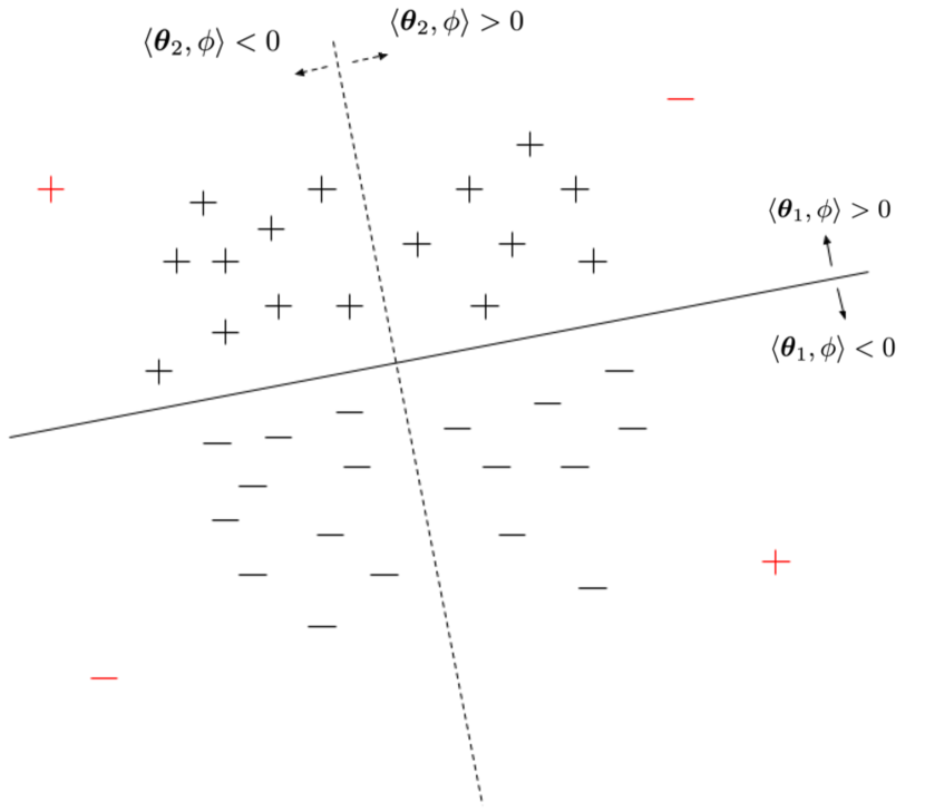
Figure 2: Pictorial illustration of the example that validates Claim 1.1. The black “$+$” and “$-$” represent positive and negative examples according to the label system induced by ${\bm{w}}_{1}$, and the solid line represents the corresponding separating hyperplane. The dashed line represents the hyperplane whose normal vector is ${\bm{w}}_{2}$, which, along with the solid line, partition that $\phi$ space into four quadrants. The red “$+$” and “$-$” represents the positive and negative examples under the new label system.

A.2 Exact integrability of the approximate ${K}^{(2)}_{t}$

In this subsection, we prove the following result:

Proposition A.2 (Exact integrability of the approximate ${K}^{(2)}_{t}$).

Assume ${\mathbf{f}}_{0}=\mathbf{0}_{n}$ , then the first three terms in RHS of (4) is equal to

$${K}^{(2)}_{0}(\bm{x},\bm{x}^{\prime})+\bigg{\langle}{K}^{(3)}_{0}(\bm{x},\bm{x}^{\prime},\cdot),({{\mathbf{K}}}^{(2)}_{0})^{-1}\bigg{(}{\mathbf{I}}_{n}-e^{-t{{\mathbf{K}}}^{(2)}_{0}/n}\bigg{)}y\bigg{\rangle}$$

$$\qquad+y^{\top}({{\mathbf{K}}}^{(2)}_{0})^{-1}\bigg{(}{\mathbf{I}}_{n}-e^{-t{{\mathbf{K}}}^{(2)}_{0}/n}\bigg{)}{K}^{(4)}_{0}(\bm{x},\bm{x}^{\prime},\cdot,\cdot)({{\mathbf{K}}}^{(2)}_{0})^{-1}y-y^{\top}{\mathbf{P}}{\mathbf{Q}}(\bm{x},\bm{x}^{\prime}){\mathbf{P}}^{\top}y,$$

where

$$\bigg{(}{\mathbf{Q}}(\bm{x},\bm{x}^{\prime})\bigg{)}_{ij}=(1-e^{-t({\mathbf{D}}_{ii}+{\mathbf{D}}_{jj})/n})\times{\bigg{(}{\mathbf{P}}^{\top}{K}^{(4)}_{0}(\bm{x},\bm{x}^{\prime},\cdot,\cdot){\mathbf{P}}{\mathbf{D}}^{-1}\bigg{)}_{ij}}\bigg{/}\bigg{(}{{\mathbf{D}}_{ii}+{\mathbf{D}}_{jj}}\bigg{)},$$

and ${\mathbf{P}}{\mathbf{D}}{\mathbf{P}}^{\top}$ is the eigen-decomposition of ${{\mathbf{K}}}^{(2)}_{0}$.

Proof.

For notational simplicity, we let ${\mathbf{H}}\equiv{{\mathbf{K}}}^{(2)}_{0}$. We have

$$\int_{0}^{t}{\mathbf{h}}_{u}-ydu =\int_{0}^{t}e^{-u{\mathbf{H}}/n}ydu=-n{\mathbf{H}}^{-1}y+n{\mathbf{H}}^{-1}e^{-t{\mathbf{H}}/n}y.$$

Hence, the second term in the RHS of (4) is

$$-\frac{1}{n}\int_{0}^{t}\bigg{\langle}{K}^{(3)}_{0},{\mathbf{h}}_{u}-y\bigg{\rangle}du=\bigg{\langle}{K}^{(3)}_{0},{\mathbf{H}}^{-1}\bigg{(}{\mathbf{I}}_{n}-e^{-t{\mathbf{H}}/n}\bigg{)}y\bigg{\rangle}.$$

We now deal with the third term in the RHS of (4). We have

$$\int_{0}^{t}\int_{0}^{u}({\mathbf{h}}_{u}-y)^{\top}{K}^{(4)}_{0}({\mathbf{h}}_{v}-y)dvdu$$

$$=y^{\top}\int_{0}^{t}\int_{0}^{u}e^{-u{\mathbf{H}}/n}{K}^{(4)}_{0}e^{-v{\mathbf{H}}/n}ydvdu$$

$$=y^{\top}\int_{0}^{t}e^{-u{\mathbf{H}}/n}{K}^{(4)}_{0}(n{\mathbf{H}}^{-1}-n{\mathbf{H}}^{-1}e^{-u{\mathbf{H}}/n})y$$

$$=n^{2}y^{\top}{\mathbf{H}}^{-1}\bigg{(}{\mathbf{I}}_{n}-e^{-t{\mathbf{H}}/n}\bigg{)}{K}^{(4)}_{0}{\mathbf{H}}^{-1}y-ny^{\top}\int_{0}^{t}e^{-u{\mathbf{H}}/n}{K}^{(4)}_{0}{\mathbf{H}}^{-1}e^{-u{\mathbf{H}}/n}ydu.$$

Let ${\mathbf{P}}{\mathbf{D}}{\mathbf{P}}^{\top}$ be an eigen-decomposition of ${\mathbf{H}}$. Then we have

$$\int_{0}^{t}e^{-u{\mathbf{H}}/n}{K}^{(4)}_{0}{\mathbf{H}}^{-1}e^{-u{\mathbf{H}}/n}du =\int_{0}^{t}{\mathbf{P}}e^{-u{\mathbf{D}}/n}\underbrace{{\mathbf{P}}^{\top}{K}^{(4)}_{0}{\mathbf{P}}{\mathbf{D}}^{-1}}_{:={\mathbf{M}}}e^{-u{\mathbf{D}}/n}{\mathbf{P}}^{\top}du$$

$$={\mathbf{P}}\int_{0}^{t}e^{-t{\mathbf{D}}/n}{\mathbf{M}}e^{-{\mathbf{D}}/n}du{\mathbf{P}}^{\top}.$$

Note that

$$\bigg{(}e^{-t{\mathbf{D}}/n}{\mathbf{M}}e^{-{\mathbf{D}}/n}\bigg{)}_{ij}={\mathbf{M}}_{ij}e^{-u(d_{i}+d_{j})/n},$$

here $d_{i}:={\mathbf{D}}_{ii}$. Hence,

$$\int_{0}^{t}\bigg{(}e^{-t{\mathbf{D}}/n}{\mathbf{M}}e^{-{\mathbf{D}}/n}\bigg{)}_{ij}du={\mathbf{M}}_{ij}\cdot\bigg{(}\frac{n}{d_{i}+d_{j}}-\frac{n}{d_{i}+d_{j}}e^{-t(d_{i}+d_{j})/n}\bigg{)},$$

which yields

$$\int_{0}^{t}e^{-u{\mathbf{H}}/n}{K}^{(4)}_{0}{\mathbf{H}}^{-1}e^{-u{\mathbf{H}}/n}du=n{\mathbf{P}}{\mathbf{Q}}{\mathbf{P}}^{\top}.$$

Putting the above equations together gives the desired result. ∎

A.3 Proof of Lemma 2.2

Note that the finite variance assumption in the definition of ${\mathcal{G}}_{A}$ is vacuous, because our label is binary. The rest of the proof is standard (see, e.g., Section 11.4 of Van der Vaart 2000).

A.4 Proof of Theorem 2.1

Assumption A.

There exists a small constant $c>0$ such that $c<\|\bm{x}_{i}\|_{2}\leq c^{-1}$ for all $i\in[n]$. Moreover, there exists an integer $p\geq 4$ such that for any $1\leq r\leq 2p+1$, the following two things happen:

1. the activation function has a bounded $r$-th derivative;

2. there exists a constant $c_{r}>0$ such that for any distinct indices $1\leq\alpha_{1},\alpha_{2},\cdots,\alpha_{r}\leq n$, the smallest singular value of the data matrix $[\bm{x}_{\alpha_{1}},\bm{x}_{\alpha_{2}},\cdots,\bm{x}_{\alpha_{r}}]$ is at least $c_{r}$.

To prove Theorem 2.1, we first collect some useful details into the following lemma.

Lemma A.3.

Under the assumptions of Theorem 2.1, with high probability, for any $u\leq t$, we have

$$\|{K}^{(3)}_{u}\|_{\infty} =\tilde{O}\bigg{(}\frac{1+u}{m}\bigg{)},\ \ \ \|{K}^{(4)}_{u}\|_{\infty}=\tilde{O}\bigg{(}\frac{1}{m}\bigg{)},\ \ \ \|K_{u}^{(5)}\|_{\infty}=\tilde{O}\bigg{(}\frac{1+u}{m^{2}}\bigg{)},$$

$$\|{\mathbf{f}}_{u}-{\mathbf{h}}_{u}\|_{2} \lesssim\frac{u(1+u)\sqrt{n}}{{m}}\bigg{(}u\land\frac{n}{\lambda}\bigg{)},\ \ \ \|{\mathbf{f}}_{u}-y\|_{2}=O(\sqrt{n}).$$

Proof.

This is implied by Equations (C.12), (C.13), (C.16), and (C.28) in Huang & Yau (2019). ∎

We are now ready to present the proof.

Proof of Theorem 2.1.

We have

$${K}^{(2)}_{t}(\bm{x}_{\alpha},\bm{x}_{\beta})$$

$$={K}^{(2)}_{0}(\bm{x}_{\alpha},\bm{x}_{\beta})-\frac{1}{n}\bigg{\langle}{K}^{(3)}_{0},\int_{0}^{t}{\mathbf{h}}_{u}-y+{\mathbf{f}}_{u}-{\mathbf{h}}_{u}du\bigg{\rangle}$$

$$\ \ \ +\frac{1}{n^{2}}\int_{0}^{t}\int_{0}^{u}({\mathbf{h}}_{u}-y+{\mathbf{f}}_{u}-{\mathbf{h}}_{u})^{\top}({K}^{(4)}_{0}+{K}^{(4)}_{v}-{K}^{(4)}_{0})({\mathbf{h}}_{v}-y+{\mathbf{f}}_{v}-{\mathbf{h}}_{v})dvdu$$

$$={K}^{(2)}_{0}(\bm{x}_{\alpha},\bm{x}_{\beta})-\frac{1}{n}\bigg{\langle}{K}^{(3)}_{0},\int_{0}^{t}{\mathbf{h}}_{u}-ydu\bigg{\rangle}+\frac{1}{n^{2}}\int_{0}^{t}\int_{0}^{u}({\mathbf{h}}_{u}-y)^{\top}{K}^{(4)}_{0}({\mathbf{h}}_{v}-y)dvdu+{\mathcal{E}},$$

where the error term ${\mathcal{E}}$ is given by

$${\mathcal{E}} =-\frac{1}{n}\bigg{\langle}{K}^{(3)}_{0},\int_{0}^{t}{\mathbf{f}}_{u}-{\mathbf{h}}_{u}du\bigg{\rangle}+\frac{1}{n^{2}}\int_{0}^{t}\int_{0}^{u}({\mathbf{h}}_{u}-y)^{\top}{K}^{(4)}_{0}({\mathbf{f}}_{v}-{\mathbf{h}}_{v})dvdu$$

$$\qquad+\frac{1}{n^{2}}\int_{0}^{t}\int_{0}^{u}({\mathbf{h}}_{u}-y)^{\top}({K}^{(4)}_{v}-{K}^{(4)}_{0})({\mathbf{f}}_{v}-y)dvdu$$

$$\qquad+\frac{1}{n^{2}}\int_{0}^{t}\int_{0}^{u}({\mathbf{f}}_{u}-{\mathbf{h}}_{u})^{\top}{K}^{(4)}_{v}({\mathbf{f}}_{v}-y)dvdu.$$

We label the four terms in the RHS above as $\textup{I},\textup{II},\textup{III}$, and IV. By lemma A.3, for the first term, w.h.p. we have

I $$\leq\frac{1}{n}\|{K}^{(3)}_{0}(\bm{x}_{\alpha},\bm{x}_{\beta},\cdot)\|_{2}\cdot\int_{0}^{t}\|{\mathbf{f}}_{u}-{\mathbf{h}}_{u}\|_{2}du$$

$$\lesssim\frac{1}{{m}}\|{K}^{(3)}_{0}\|_{\infty}\cdot\int_{0}^{t}u(1+u)\bigg{(}u\land\frac{n}{\lambda}\bigg{)}du$$

$$\lesssim\frac{(\log m)^{c}}{m^{2}}\cdot\bigg{(}(t^{3}+t^{4})\land\frac{n(t^{2}+t^{3})}{\lambda}\bigg{)}$$

$$\lesssim\frac{(\log m)^{c}\cdot t^{2}(1+t)}{m^{2}}\bigg{(}t\land\frac{n}{\lambda}\bigg{)}.$$

For the second term, we have

II $$\leq\frac{1}{n^{2}}\int_{0}^{t}\int_{0}^{u}\|{\mathbf{h}}_{u}-y\|_{2}\|{\mathbf{f}}_{v}-{\mathbf{h}}_{v}\|_{2}\|{K}^{(4)}_{0}(\bm{x}_{\alpha},\bm{x}_{\beta},\cdot,\cdot)\|dvdu$$

$$\lesssim\frac{1}{m}\int_{0}^{t}\int_{0}^{u}v(1+v)\bigg{(}v\land\frac{n}{\lambda}\bigg{)}\|{K}^{(4)}_{0}\|_{\infty}dvdu$$

$$\lesssim\frac{(\log m)^{c}}{m^{2}}\int_{0}^{t}\int_{0}^{u}v(1+v)\bigg{(}v\land\frac{n}{\lambda}\bigg{)}$$

$$\lesssim\frac{(\log m)^{c}}{m^{2}}(t^{4}+t^{5})\land\frac{n(t^{3}+t^{4})}{\lambda}$$

$$=\frac{(\log m)^{c}\cdot t^{3}(1+t)}{m^{2}}\bigg{(}t\land\frac{n}{\lambda}\bigg{)}.$$

For the third term, we have

III $$\leq\frac{1}{n^{2}}\int_{0}^{t}\int_{0}^{u}\|{\mathbf{h}}_{u}-y\|_{2}\|{\mathbf{f}}_{v}-y\|_{2}\|{K}^{(4)}_{v}(\bm{x}_{\alpha},\bm{x}_{\beta},\cdot,\cdot)-{K}^{(4)}_{0}(\bm{x}_{\alpha},\bm{x}_{\beta},\cdot,\cdot)\|_{2}dvdu.$$

Note that

$$\|{\mathbf{h}}_{u}-y\|_{2} \leq\|{\mathbf{h}}_{u}-{\mathbf{f}}_{u}\|_{2}+\|{\mathbf{f}}_{u}-y\|_{2}\lesssim\frac{u(1+u)\sqrt{n}}{m}\bigg{(}u\land\frac{n}{\lambda}\bigg{)}+\sqrt{n},$$

$$\|{\mathbf{f}}_{v}-y\|_{2} \lesssim\sqrt{n},$$

and

$$\|{K}^{(4)}_{v}(\bm{x}_{\alpha},\bm{x}_{\beta},\cdot,\cdot)-{K}^{(4)}_{0}(\bm{x}_{\alpha},\bm{x}_{\beta},\cdot,\cdot)\|_{2}$$

$$\leq n\max_{i,j\in[n]}|{K}^{(4)}_{v}(\bm{x}_{\alpha},\bm{x}_{\beta},\bm{x}_{i},\bm{x}_{j})-{K}^{(4)}_{0}(\bm{x}_{\alpha},\bm{x}_{\beta},\bm{x}_{i},\bm{x}_{j})|$$

$$\leq n\int_{0}^{v}\max_{i,j\in[n]}|\dot{K}_{w}^{(4)}(\bm{x}_{\alpha},\bm{x}_{\beta},\bm{x}_{i},\bm{x}_{j})|dw$$

$$=n\int_{0}^{v}\max_{i,j\in[n]}\frac{1}{n}\bigg{|}\sum_{k\in[n]}K^{(5)}_{w}(\bm{x}_{\alpha},\bm{x}_{\beta},\bm{x}_{i},\bm{x}_{j},\bm{x}_{k})(f_{w}(\bm{x}_{k})-y_{k})\bigg{|}dw$$

$$\leq n\int_{0}^{v}\|K^{(5)}_{w}\|_{\infty}\frac{1}{\sqrt{n}}\|{\mathbf{f}}_{w}-y\|_{2}dw$$

$$\lesssim\frac{n(\log m)^{c}}{m^{2}}\int_{0}^{v}(1+w)dw$$

$$\lesssim\frac{n(\log m)^{c}\cdot(v+v^{2})}{m^{2}}.$$

Hence, we can bound the third term by

III $$\lesssim\frac{(\log m)^{c}}{m^{2}}\int_{0}^{t}\int_{0}^{u}(v+v^{2})\bigg{(}1+\frac{u(1+u)(u\land n/\lambda)}{m}\bigg{)}dvdu$$

$$\lesssim\frac{(\log m)^{c}\cdot t^{3}(1+t)}{m^{2}}+\frac{(\log m)^{c}\cdot t^{4}(1+t+t^{2})}{m^{3}}\bigg{(}t\land\frac{n}{\lambda}\bigg{)}.$$

Finally, we bound the fourth term by

IV $$\leq\frac{1}{n^{2}}\int_{0}^{t}\int_{0}^{u}\|{\mathbf{f}}_{u}-{\mathbf{h}}_{u}\|_{2}\|{\mathbf{f}}_{v}-y\|_{2}\|{K}^{(4)}_{v}(\bm{x}_{\alpha},\bm{x}_{\beta},\cdot,\cdot)\|_{2}dvdu$$

$$\lesssim\frac{(\log m)^{c}}{m^{2}}\int_{0}^{t}\int_{0}^{u}u(1+u)\bigg{(}u\land\frac{n}{\lambda}\bigg{)}dvdu$$

$$\lesssim\frac{(\log m)^{c}\cdot t^{3}(1+t)}{m^{2}}\bigg{(}t\land\frac{n}{\lambda}\bigg{)}.$$

Combining the above four bounds gives the desired bound on ${\mathcal{E}}$. The bounds for the three terms in the RHS of (4) are derived similarly, and we omit the details. ∎

Appendix B NTH-Related Calculations

B.1 An Symbolic Program to Compute NTH

In this section, we develop a recursive program to symbolically compute $K^{(r)}_{t}$, the $r$-th order kernel in NTH. For simplicity, we consider neural nets without biases :

$$f(\bm{x},{\bm{w}})={\mathbf{W}}^{{}(L)}\sigma\bigg{(}{\mathbf{W}}^{{}(L-1)}\cdots\bigl{(}{\mathbf{W}}^{{}(2)}\sigma({\mathbf{W}}^{{}(1)}\bm{x})\bigr{)}\bigg{)}.$$

We begin by noting that $K^{(2)}_{t}$ can be written as an inner product of two gradients. We will see that $K^{(3)}_{t}$ can be written as a quadratic form, and $K^{(4)}$ can be written as a cubic form, etc.

To this end, let us denote $\nabla f(\bm{x},{\bm{w}})$ to be the partial derivative of $f(\bm{x},{\bm{w}})$ w.r.t. ${\bm{w}}$. We sometimes drop the dependence on $t$ and write $f(\bm{x}_{\alpha},{\bm{w}}_{t})\equiv f_{\alpha}$ when there is no ambiguity.

We will regard ${\bm{w}}={\mathbf{W}}=\{{\mathbf{W}}^{(\ell)}_{jk}:\ell\in[L],j\in[p_{\ell}],j\in[q_{\ell}]\}$ as a rank-$3$ tensor. We write ${\mathbf{W}}^{{}(\ell)}_{jk}\equiv{\mathbf{W}}_{\ell jk}$ when there is no ambiguity. In our current notations, $\nabla f(\bm{x},{\bm{w}})=\{\bigl{(}\nabla f(\bm{x},{\bm{w}})\bigr{)}_{\ell jk}:\ell\in[L],j\in p_{\ell},k\in q_{\ell}\}$ is also a rank-$3$ tensor. We begin by writing

$${K}^{(2)}_{t}(\bm{x}_{\alpha},\bm{x}_{\beta}) =\langle\nabla f(\bm{x}_{\alpha},{\bm{w}}_{t}),\nabla f(\bm{x}_{\beta},{\bm{w}}_{t})\rangle$$

$$=\sum_{\ell\in[L]}\sum_{j\in[p_{\ell}]}\sum_{k\in[q_{\ell}]}\frac{\partial f(\bm{x}_{\alpha},{\bm{w}}_{t})}{\partial{\mathbf{W}}^{{}(\ell)}_{jk}}\cdot\frac{\partial f(\bm{x}_{\beta},{\bm{w}}_{t})}{\partial{\mathbf{W}}^{{}(\ell)}_{jk}}$$

$$=(\nabla f_{\alpha})^{\ell jk}(\nabla f_{\beta})_{\ell jk},$$

where in the last line we have used the Einstein notation . Taking derivative w.r.t. $t$ gives

$$\frac{d}{dt}{K}^{(2)}_{t}(\bm{x}_{\alpha},\bm{x}_{\beta}) =(\frac{d}{dt}\nabla f_{\alpha})^{\ell jk}(\nabla f_{\beta})_{\ell jk}+(\nabla f_{\alpha})^{\ell jk}(\frac{d}{dt}\nabla f_{\beta})_{\ell jk}.$$

We have

$$(\frac{d}{dt}\nabla f_{\alpha})_{\ell jk} =\frac{\partial(\nabla f_{\alpha})_{\ell jk}}{\partial{\mathbf{W}}_{suv}}\cdot\frac{d{\mathbf{W}}_{suv}}{dt}$$

$$=\frac{\partial(\nabla f_{\alpha})_{\ell jk}}{\partial{\mathbf{W}}_{suv}}\cdot{\frac{-dL({\bm{w}}_{t})}{d{\mathbf{W}}_{suv}}}$$

$$=\frac{\partial(\nabla f_{\alpha})_{\ell jk}}{\partial{\mathbf{W}}_{suv}}\cdot\bigg{(}-\frac{1}{n}\sum_{\gamma\in[n]}(f_{\gamma}-y_{\gamma})\cdot(\nabla f_{\gamma})_{suv}\bigg{)}$$

$$=-\frac{1}{n}\sum_{\gamma\in[n]}(f_{\gamma}-y_{\gamma})\cdot\frac{\partial(\nabla f_{\alpha})_{\ell jk}}{\partial{\mathbf{W}}_{suv}}\cdot(\nabla f_{\gamma})_{suv}$$

$${=}-\frac{1}{n}\sum_{\gamma\in[n]}(f_{\gamma}-y_{\gamma})\cdot(\nabla^{2}f_{\alpha})^{\ell jk}_{suv}\cdot(\nabla f_{\gamma})_{suv},$$

where we denote $\nabla^{2}f$ to be the rank-$6$ tensor, whose $(\ell,j,k,s,u,v)$-th entry is given by

$${\partial}(\nabla f)_{\ell jk}/\partial{\mathbf{W}}_{suv}=\frac{\partial^{2}f}{\partial{\mathbf{W}}_{suv}{\mathbf{W}}_{\ell jk}}.$$

A similar computation gives

$$(\frac{d}{dt}\nabla f_{\beta})_{\ell jk}=-\frac{1}{n}\sum_{\gamma\in[n]}(f_{\gamma}-y_{\gamma})\cdot(\nabla^{2}f_{\beta})^{\ell jk}_{suv}\cdot(\nabla f_{\gamma})_{suv}.$$

Hence, we arrive at

$${K}^{(3)}_{t}(\bm{x}_{\alpha},\bm{x}_{\beta},\bm{x}_{\gamma})$$

$$=(\nabla^{2}f_{\alpha})^{\ell jk}_{suv}(\nabla f_{\beta})_{\ell jk}(\nabla f_{\gamma})_{suv}+(\nabla f_{\alpha})_{\ell jk}(\nabla^{2}f_{\beta})^{\ell jk}_{suv}(\nabla f_{\gamma})_{suv}$$

$$=\sum_{\ell\in[L]}\sum_{j\in[p_{\ell}]}\sum_{k\in[q_{\ell}]}\sum_{s\in[L]}\sum_{u\in[p_{s}]}\sum_{v\in[q_{s}]}\frac{\partial f(\bm{x}_{\beta},{\bm{w}}_{t})}{\partial{\mathbf{W}}_{\ell jk}}\cdot\frac{\partial^{2}f(\bm{x}_{\alpha},{\bm{w}}_{t})}{\partial{\mathbf{W}}_{\ell jk}\partial{\mathbf{W}}_{suv}}\cdot\frac{\partial f(\bm{x}_{\gamma},{\bm{w}}_{t})}{{\partial}{\mathbf{W}}_{suv}}$$

$$\qquad+\frac{\partial f(\bm{x}_{\alpha},{\bm{w}}_{t})}{\partial{\mathbf{W}}_{\ell jk}}\cdot\frac{\partial^{2}f(\bm{x}_{\beta},{\bm{w}}_{t})}{\partial{\mathbf{W}}_{\ell jk}\partial{\mathbf{W}}_{suv}}\cdot\frac{\partial f(\bm{x}_{\gamma},{\bm{w}}_{t})}{{\partial}{\mathbf{W}}_{suv}}.$$

Note that the above expression is a quadratic form:

$${K}^{(3)}_{t}(\bm{x}_{\alpha},\bm{x}_{\beta},\bm{x}_{\gamma})=(\nabla f_{\beta})^{\top}(\nabla^{2}f_{\alpha})(\nabla f_{\gamma})+(\nabla f_{\alpha})^{\top}(\nabla^{2}f_{\beta})(\nabla f_{\gamma}).$$

We have already seen some patterns showing up. To obtain ${K}^{(3)}_{t}$ from ${K}^{(2)}_{t}$, we simply conduct the following program:

1. Start with ${K}^{(2)}_{t}=(\nabla f_{\alpha})^{\ell jk}(\nabla f_{\beta})_{\ell jk}$ in Einstein notation, which is a function of $r=2$ gradients;

2. Introduce a new index $\gamma$ for data points, and a new set of indices $(suv)$ for weights;

3. Replicate ${K}^{(2)}_{t}$ for $r=2$ times, and append $(\nabla f_{\gamma})_{suv}$ to the end of each term:

   $$(\nabla f_{\alpha})^{\ell jk}(\nabla f_{\beta})_{\ell jk}(\nabla f_{\gamma})_{suv}+(\nabla f_{\alpha})^{\ell jk}(\nabla f_{\beta})_{\ell jk}(\nabla f_{\gamma})_{suv};$$

4. Choose a term from a total of $r=2$ terms in ${K}^{(2)}_{t}$, raise its gradient to one higher level, add the new indices $(suv)$ to this term, and do this operation in all possible ways:

   $${K}^{(3)}_{t}=(\nabla^{2}f_{\alpha})^{\ell jk}_{suv}(\nabla f_{\beta})_{\ell jk}(\nabla f_{\gamma})_{suv}+(\nabla f_{\alpha})_{\ell jk}(\nabla^{2}f_{\beta})^{\ell jk}_{suv}(\nabla f_{\gamma})_{suv}.$$

We now apply the above program to obtain ${K}^{(4)}_{t}$ from ${K}^{(3)}_{t}$:

1. Introduce a new index $\xi$ for data points, and a new set of indices $(abc)$;

2. Since ${K}^{(3)}$ is a function of $r=3$ gradients, we replicate ${K}^{(3)}_{t}$ for $3$ times, and append $(\nabla f_{\xi})_{abc}$ to the end of each term:

   $$(\nabla^{2}f_{\alpha})^{\ell jk}_{suv}(\nabla f_{\beta})_{\ell jk}(\nabla f_{\gamma})_{suv}(\nabla f_{\xi})_{abc}$$

   $$+(\nabla^{2}f_{\alpha})^{\ell jk}_{suv}(\nabla f_{\beta})_{\ell jk}(\nabla f_{\gamma})_{suv}(\nabla f_{\xi})_{abc}$$

   $$+(\nabla^{2}f_{\alpha})^{\ell jk}_{suv}(\nabla f_{\beta})_{\ell jk}(\nabla f_{\gamma})_{suv}(\nabla f_{\xi})_{abc}$$

   $$+(\nabla f_{\alpha})_{\ell jk}(\nabla^{2}f_{\beta})^{\ell jk}_{suv}(\nabla f_{\gamma})_{suv}(\nabla f_{\xi})_{abc}$$

   $$+(\nabla f_{\alpha})_{\ell jk}(\nabla^{2}f_{\beta})^{\ell jk}_{suv}(\nabla f_{\gamma})_{suv}(\nabla f_{\xi})_{abc}$$

   $$+(\nabla f_{\alpha})_{\ell jk}(\nabla^{2}f_{\beta})^{\ell jk}_{suv}(\nabla f_{\gamma})_{suv}(\nabla f_{\xi})_{abc};$$

3. Raise a term’s gradient (from the former $3$ terms) to a higher level, add the new indices, and do it in all possible ways:

   $${K}^{(4)}_{t}= (\nabla^{3}f_{\alpha})^{\ell jk}_{suv,abc}(\nabla f_{\beta})_{\ell jk}(\nabla f_{\gamma})_{suv}(\nabla f_{\xi})_{abc}$$

   $$+(\nabla^{2}f_{\alpha})^{\ell jk}_{suv}(\nabla^{2}f_{\beta})^{\ell jk}_{abc}(\nabla f_{\gamma})_{suv}(\nabla f_{\xi})_{abc}$$

   $$+(\nabla^{2}f_{\alpha})^{\ell jk}_{suv}(\nabla f_{\beta})_{\ell jk}(\nabla^{2}f_{\gamma})^{suv}_{abc}(\nabla f_{\xi})_{abc}$$

   $$+(\nabla^{2}f_{\alpha})^{\ell jk}_{abc}(\nabla^{2}f_{\beta})^{\ell jk}_{suv}(\nabla f_{\gamma})_{suv}(\nabla f_{\xi})_{abc}$$

   $$+(\nabla f_{\alpha})_{\ell jk}(\nabla^{3}f_{\beta})^{\ell jk}_{suv,abc}(\nabla f_{\gamma})_{suv}(\nabla f_{\xi})_{abc}$$

   $$+(\nabla f_{\alpha})_{\ell jk}(\nabla^{2}f_{\beta})^{\ell jk}_{suv}(\nabla^{2}f_{\gamma})^{suv}_{abc}(\nabla f_{\xi})_{abc}.$$ (11)

In the above program, we have regarded $\nabla^{3}f$ as a rank-$9$ tensor, whose $(\ell,j,k,s,u,v,a,b,c)$-th entry is given by

$$\frac{\partial^{3}f}{\partial{\mathbf{W}}_{abc}{\partial}{\mathbf{W}}_{suv}{\partial}{\mathbf{W}}_{\ell jk}}.$$

The correctness of the above recursive symbolic program can be proved by straightforward induction, and we omit the details.

B.2 Explicit Expressions for NTH for Two-Layer Nets

Taking advantage of the recursive program, it’s relatively easy to get explicit expressions for $K^{(r)}$ when $r$ is not too large. We focus on the following two-layer net

$$f(\bm{x},{\bm{w}})=\frac{1}{\sqrt{m}}{\mathbf{a}}^{\top}\sigma({\mathbf{W}}\bm{x}).$$ (12)

Proposition B.1 (Expression for ${K}^{(2)}_{t},{K}^{(3)}_{t}$ and ${K}^{(4)}_{t}$ in a two-layer net).

For the two layer neural network $f(\bm{x},{\bm{w}})=\frac{1}{\sqrt{m}}{\mathbf{a}}^{\top}\sigma({\mathbf{W}}\bm{x})$, where ${\mathbf{a}}\in{\mathbb{R}}^{m},{\mathbf{W}}\in{\mathbb{R}}^{m\times d}$, and $\sigma$ an activation function, we have

$${K}^{(2)}_{t}(\bm{x}_{\alpha},\bm{x}_{\beta})$$

$$=\frac{1}{m}\bm{x}_{\alpha}^{\top}\bm{x}_{\beta}\cdot\bigg{\langle}\sigma^{\prime}({\mathbf{W}}\bm{x}_{\alpha})\odot{\mathbf{a}}_{t},\sigma^{\prime}({\mathbf{W}}\bm{x}_{\beta})\odot{\mathbf{a}}_{t}\bigg{\rangle}+\frac{1}{m}\bigg{\langle}\sigma({\mathbf{W}}\bm{x}_{\alpha}),\sigma({\mathbf{W}}\bm{x}_{\beta})\bigg{\rangle},$$ (13)

$${K}^{(3)}_{t}(\bm{x}_{\alpha},\bm{x}_{\beta},\bm{x}_{\gamma})$$

$$=\frac{1}{m\sqrt{m}}\bm{x}_{\alpha}^{\top}\bm{x}_{\gamma}\cdot\bm{x}_{\alpha}^{\top}\bm{x}_{\beta}\cdot\bigg{\langle}{\mathbf{a}}_{t}\odot{\mathbf{a}}_{t}\odot{\mathbf{a}}_{t},\sigma^{\prime\prime}({\mathbf{W}}\bm{x}_{\alpha})\odot\sigma^{\prime}({\mathbf{W}}\bm{x}_{\beta})\odot\sigma^{\prime}({\mathbf{W}}\bm{x}_{\gamma})\bigg{\rangle}$$

$$\qquad+\frac{1}{m\sqrt{m}}\bm{x}_{\beta}^{\top}\bm{x}_{\gamma}\cdot\bm{x}_{\alpha}^{\top}\bm{x}_{\beta}\cdot\bigg{\langle}{\mathbf{a}}_{t}\odot{\mathbf{a}}_{t}\odot{\mathbf{a}}_{t},\sigma^{\prime}({\mathbf{W}}\bm{x}_{\alpha})\odot\sigma^{\prime\prime}({\mathbf{W}}\bm{x}_{\beta})\odot\sigma^{\prime}({\mathbf{W}}\bm{x}_{\gamma})\bigg{\rangle}$$

$$\qquad+\frac{2}{m\sqrt{m}}\bm{x}_{\alpha}^{\top}\bm{x}_{\beta}\cdot\bigg{\langle}{\mathbf{a}}_{t},\sigma^{\prime}({\mathbf{W}}\bm{x}_{\alpha})\odot\sigma^{\prime}({\mathbf{W}}\bm{x}_{\beta})\odot\sigma({\mathbf{W}}\bm{x}_{\gamma})\bigg{\rangle}$$

$$\qquad+\frac{1}{m\sqrt{m}}\bm{x}_{\alpha}^{\top}\bm{x}_{\gamma}\cdot\bigg{\langle}{\mathbf{a}}_{t},\sigma^{\prime}({\mathbf{W}}\bm{x}_{\alpha})\odot\sigma({\mathbf{W}}\bm{x}_{\beta})\odot\sigma^{\prime}({\mathbf{W}}\bm{x}_{\gamma})\bigg{\rangle}$$

$$\qquad+\frac{1}{m\sqrt{m}}\bm{x}_{\beta}^{\top}\bm{x}_{\gamma}\cdot\bigg{\langle}{\mathbf{a}}_{t},\sigma({\mathbf{W}}\bm{x}_{\alpha})\odot\sigma^{\prime}({\mathbf{W}}\bm{x}_{\beta})\odot\sigma^{\prime}({\mathbf{W}}\bm{x}_{\gamma})\bigg{\rangle},$$ (14)

$${K}^{(4)}_{t}(\bm{x}_{\alpha},\bm{x}_{\beta},\bm{x}_{\gamma},\bm{x}_{\xi})$$

$$=\frac{1}{m^{2}}\bm{x}_{\alpha}^{\top}\bm{x}_{\beta}\cdot\bm{x}_{\alpha}^{\top}\bm{x}_{\gamma}\cdot\bm{x}_{\alpha}^{\top}\bm{x}_{\xi}\cdot\bigg{\langle}{\mathbf{a}}_{t}^{\odot 4},\sigma^{\prime\prime\prime}({\mathbf{W}}\bm{x}_{\alpha})\odot\sigma^{\prime}({\mathbf{W}}\bm{x}_{\beta})\odot\sigma^{\prime}({\mathbf{W}}\bm{x}_{\gamma})\odot\sigma^{\prime}({\mathbf{W}}\bm{x}_{\xi})\bigg{\rangle}$$

$$+\frac{1}{m^{2}}\bm{x}_{\beta}^{\top}\bm{x}_{\alpha}\cdot\bm{x}_{\beta}^{\top}\bm{x}_{\gamma}\cdot\bm{x}_{\beta}^{\top}\bm{x}_{\xi}\cdot\bigg{\langle}{\mathbf{a}}_{t}^{\odot 4},\sigma^{\prime}({\mathbf{W}}\bm{x}_{\alpha})\odot\sigma^{\prime\prime\prime}({\mathbf{W}}\bm{x}_{\beta})\odot\sigma^{\prime}({\mathbf{W}}\bm{x}_{\gamma})\odot\sigma^{\prime}({\mathbf{W}}\bm{x}_{\xi})\bigg{\rangle}$$

$$+\frac{1}{m^{2}}\bm{x}_{\alpha}^{\top}\bm{x}_{\beta}\cdot(\bm{x}_{\alpha}^{\top}\bm{x}_{\gamma}\cdot\bm{x}_{\beta}^{\top}\bm{x}_{\xi}+\bm{x}_{\alpha}^{\top}\bm{x}_{\xi}\cdot\bm{x}_{\beta}^{\top}\bm{x}_{\gamma})\cdot\bigg{\langle}{\mathbf{a}}^{\odot 4},\sigma^{\prime\prime}({\mathbf{W}}\bm{x}_{\alpha})\odot\sigma^{\prime\prime}({\mathbf{W}}\bm{x}_{\beta})\odot\sigma^{\prime}({\mathbf{W}}\bm{x}_{\gamma})\odot\sigma^{\prime}({\mathbf{W}}\bm{x}_{\xi})\bigg{\rangle}$$

$$+\frac{1}{m^{2}}\bm{x}_{\alpha}^{\top}\bm{x}_{\gamma}\cdot\bm{x}_{\alpha}^{\top}\bm{x}_{\beta}\cdot\bm{x}_{\gamma}^{\top}\bm{x}_{\xi}\cdot\bigg{\langle}{\mathbf{a}}^{\odot 4},\sigma^{\prime\prime}({\mathbf{W}}\bm{x}_{\alpha})\odot\sigma^{\prime}({\mathbf{W}}\bm{x}_{\beta})\odot\sigma^{\prime\prime}({\mathbf{W}}\bm{x}_{\gamma})\odot\sigma^{\prime}({\mathbf{W}}\bm{x}_{\xi})\bigg{\rangle}$$

$$+\frac{1}{m^{2}}\bm{x}_{\beta}^{\top}\bm{x}_{\gamma}\cdot\bm{x}_{\beta}^{\top}\bm{x}_{\alpha}\cdot\bm{x}_{\gamma}^{\top}\bm{x}_{\xi}\cdot\bigg{\langle}{\mathbf{a}}^{\odot 4},\sigma^{\prime}({\mathbf{W}}\bm{x}_{\alpha})\odot\sigma^{\prime\prime}({\mathbf{W}}\bm{x}_{\beta})\odot\sigma^{\prime\prime}({\mathbf{W}}\bm{x}_{\gamma})\odot\sigma^{\prime}({\mathbf{W}}\bm{x}_{\xi})\bigg{\rangle}$$

$$+\frac{3}{m^{2}}\bm{x}_{\alpha}^{\top}\bm{x}_{\beta}\cdot\bm{x}_{\alpha}^{\top}\bm{x}_{\gamma}\cdot\bigg{\langle}{\mathbf{a}}^{\odot 2},\sigma^{\prime\prime}({\mathbf{W}}\bm{x}_{\alpha})\odot\sigma^{\prime}({\mathbf{W}}\bm{x}_{\beta})\odot\sigma^{\prime}({\mathbf{W}}\bm{x}_{\gamma})\odot\sigma({\mathbf{W}}\bm{x}_{\xi})\bigg{\rangle}$$

$$+\frac{3}{m^{2}}\bm{x}_{\beta}^{\top}\bm{x}_{\alpha}\cdot\bm{x}_{\beta}^{\top}\bm{x}_{\gamma}\cdot\bigg{\langle}{\mathbf{a}}^{\odot 2},\sigma^{\prime}({\mathbf{W}}\bm{x}_{\alpha})\odot\sigma^{\prime\prime}({\mathbf{W}}\bm{x}_{\beta})\odot\sigma^{\prime}({\mathbf{W}}\bm{x}_{\gamma})\odot\sigma({\mathbf{W}}\bm{x}_{\xi})\bigg{\rangle}$$

$$+\frac{2}{m^{2}}\bm{x}_{\alpha}^{\top}\bm{x}_{\beta}\cdot\bm{x}_{\alpha}^{\top}\bm{x}_{\xi}\cdot\bigg{\langle}{\mathbf{a}}^{\odot 2},\sigma^{\prime\prime}({\mathbf{W}}\bm{x}_{\alpha})\odot\sigma^{\prime}({\mathbf{W}}\bm{x}_{\beta})\odot\sigma({\mathbf{W}}\bm{x}_{\gamma})\odot\sigma^{\prime}({\mathbf{W}}\bm{x}_{\xi})\bigg{\rangle}$$

$$+\frac{2}{m^{2}}\bm{x}_{\beta}^{\top}\bm{x}_{\alpha}\cdot\bm{x}_{\beta}^{\top}\bm{x}_{\xi}\cdot\bigg{\langle}{\mathbf{a}}^{\odot 2},\sigma^{\prime}({\mathbf{W}}\bm{x}_{\alpha})\odot\sigma^{\prime\prime}({\mathbf{W}}\bm{x}_{\beta})\odot\sigma({\mathbf{W}}\bm{x}_{\gamma})\odot\sigma^{\prime}({\mathbf{W}}\bm{x}_{\xi})\bigg{\rangle}$$

$$+\frac{2}{m^{2}}\bm{x}_{\alpha}^{\top}\bm{x}_{\beta}\cdot\bm{x}_{\gamma}^{\top}\bm{x}_{\xi}\cdot\bigg{\langle}{\mathbf{a}}^{\odot 2},\sigma^{\prime}({\mathbf{W}}\bm{x}_{\alpha})\odot\sigma^{\prime}({\mathbf{W}}\bm{x}_{\beta})\odot\sigma^{\prime}({\mathbf{W}}\bm{x}_{\gamma})\odot\sigma^{\prime}({\mathbf{W}}\bm{x}_{\xi})\bigg{\rangle}$$

$$+\frac{1}{m^{2}}\bm{x}_{\alpha}^{\top}\bm{x}_{\gamma}\cdot\bm{x}_{\alpha}^{\top}\bm{x}_{\xi}\cdot\bigg{\langle}{\mathbf{a}}^{\odot 2},\sigma^{\prime\prime}({\mathbf{W}}\bm{x}_{\alpha})\odot\sigma({\mathbf{W}}\bm{x}_{\beta})\odot\sigma^{\prime}({\mathbf{W}}\bm{x}_{\gamma})\odot\sigma^{\prime}({\mathbf{W}}\bm{x}_{\xi})\bigg{\rangle}$$

$$+\frac{1}{m^{2}}\bm{x}_{\gamma}^{\top}\bm{x}_{\alpha}\cdot\bm{x}_{\gamma}^{\top}\bm{x}_{\xi}\cdot\bigg{\langle}{\mathbf{a}}^{\odot 2},\sigma^{\prime}({\mathbf{W}}\bm{x}_{\alpha})\odot\sigma({\mathbf{W}}\bm{x}_{\beta})\odot\sigma^{\prime\prime}({\mathbf{W}}\bm{x}_{\gamma})\odot\sigma^{\prime}({\mathbf{W}}\bm{x}_{\xi})\bigg{\rangle}$$

$$+\frac{1}{m^{2}}\bm{x}_{\beta}^{\top}\bm{x}_{\gamma}\cdot\bm{x}_{\beta}^{\top}\bm{x}_{\xi}\cdot\bigg{\langle}{\mathbf{a}}^{\odot 2},\sigma({\mathbf{W}}\bm{x}_{\alpha})\odot\sigma^{\prime\prime}({\mathbf{W}}\bm{x}_{\beta})\odot\sigma^{\prime}({\mathbf{W}}\bm{x}_{\gamma})\odot\sigma^{\prime}({\mathbf{W}}\bm{x}_{\xi})\bigg{\rangle}$$

$$+\frac{1}{m^{2}}\bm{x}_{\gamma}^{\top}\bm{x}_{\beta}\cdot\bm{x}_{\gamma}^{\top}\bm{x}_{\xi}\cdot\bigg{\langle}{\mathbf{a}}^{\odot 2},\sigma({\mathbf{W}}\bm{x}_{\alpha})\odot\sigma^{\prime}({\mathbf{W}}\bm{x}_{\beta})\odot\sigma^{\prime\prime}({\mathbf{W}}\bm{x}_{\gamma})\odot\sigma^{\prime}({\mathbf{W}}\bm{x}_{\xi})\bigg{\rangle}$$

$$+\frac{1}{m^{2}}(\bm{x}_{\alpha}^{\top}\bm{x}_{\gamma}\cdot\bm{x}_{\beta}^{\top}\bm{x}_{\xi}+\bm{x}_{\alpha}^{\top}\bm{x}_{\xi}\cdot\bm{x}_{\beta}^{\top}\bm{x}_{\gamma})\cdot\bigg{\langle}{\mathbf{a}}^{\odot 2},\sigma^{\prime}({\mathbf{W}}\bm{x}_{\alpha})\odot\sigma^{\prime}({\mathbf{W}}\bm{x}_{\beta})\odot\sigma^{\prime}({\mathbf{W}}\bm{x}_{\gamma})\odot\sigma^{\prime}({\mathbf{W}}\bm{x}_{\xi})\bigg{\rangle}$$

$$+\frac{2}{m^{2}}\bm{x}_{\alpha}^{\top}\bm{x}_{\beta}\cdot\bigg{\langle}\mathbf{1}_{m},\sigma^{\prime}({\mathbf{W}}\bm{x}_{\alpha})\odot\sigma^{\prime}({\mathbf{W}}\bm{x}_{\beta})\odot\sigma({\mathbf{W}}\bm{x}_{\gamma})\odot\sigma({\mathbf{W}}\bm{x}_{\xi})\bigg{\rangle}$$

$$+\frac{1}{m^{2}}\bm{x}_{\alpha}^{\top}\bm{x}_{\gamma}\cdot\bigg{\langle}\mathbf{1}_{m},\sigma^{\prime}({\mathbf{W}}\bm{x}_{\alpha})\odot\sigma({\mathbf{W}}\bm{x}_{\beta})\odot\sigma^{\prime}({\mathbf{W}}\bm{x}_{\gamma})\odot\sigma({\mathbf{W}}\bm{x}_{\xi})\bigg{\rangle}$$

$$+\frac{1}{m^{2}}\bm{x}_{\beta}^{\top}\bm{x}_{\gamma}\cdot\bigg{\langle}\mathbf{1}_{m},\sigma({\mathbf{W}}\bm{x}_{\alpha})\odot\sigma^{\prime}({\mathbf{W}}\bm{x}_{\beta})\odot\sigma^{\prime}({\mathbf{W}}\bm{x}_{\gamma})\odot\sigma({\mathbf{W}}\bm{x}_{\xi})\bigg{\rangle},$$ (15)

where we let ${\mathbf{a}}^{\odot r}$ to be the vector whose $i$-th entry is ${\mathbf{a}}_{i}^{r}$.

Proof.

Computation of ${K}^{(2)}_{t}$. We first compute ${K}^{(2)}_{t}(\bm{x}_{\alpha},\bm{x}_{\beta})=(\nabla f_{\alpha})_{\ell jk}(\nabla f_{\beta})_{\ell jk}$. We have

$$\frac{\partial f(\bm{x},{\bm{w}})}{\partial{\mathbf{a}}} =\frac{1}{\sqrt{m}}\sigma({\mathbf{W}}\bm{x})$$

$$\frac{\partial f(\bm{x},{\bm{w}})}{\partial{\mathbf{W}}} =\frac{1}{\sqrt{m}}\operatorname{diag}(\sigma^{\prime}({\mathbf{W}}\bm{x}){\mathbf{a}}\bm{x}^{\top}=\frac{1}{\sqrt{m}}\bigg{(}\sigma^{\prime}({\mathbf{W}}\bm{x}\odot{\mathbf{a}})\bigg{)}x^{\top}.$$

Then Equation (13) follows by trivial algebra.

Computation of ${K}^{(3)}_{t}$. Now consider ${K}^{(3)}_{t}$. We have

$${K}^{(3)}_{t}(\bm{x}_{\alpha},\bm{x}_{\beta},\bm{x}_{\gamma})=(\nabla^{2}f_{\alpha})^{\ell jk}_{suv}(\nabla f_{\beta})_{\ell jk}(\nabla f_{\gamma})_{suv}+(\nabla f_{\alpha})_{\ell jk}(\nabla^{2}f_{\beta})^{\ell jk}_{suv}(\nabla f_{\gamma})_{suv}.$$

For the $\ell=s=2$ term, we have $(\nabla^{2}f)^{2jk}_{2uv}=0$, since $\partial f/\partial{\mathbf{a}}$ is constant in ${\mathbf{a}}$. For the $\ell=s=1$ term, we have

$$(\nabla^{2}f)^{1jk}_{1uv} =\frac{\partial^{2}f(\bm{x},{\bm{w}})}{\partial{\mathbf{W}}_{uv}W_{jk}}$$

$$=\frac{\partial}{\partial{\mathbf{W}}_{uv}}\frac{1}{\sqrt{m}}\sigma^{\prime}({\mathbf{W}}\bm{x}_{j}){\mathbf{a}}_{j}\bm{x}_{k}$$

$$=\frac{1}{\sqrt{m}}\sigma^{\prime\prime}({\mathbf{W}}\bm{x}_{j})\delta_{ju}\bm{x}_{v}{\mathbf{a}}_{j}\bm{x}_{k},$$

where $\delta_{ju}$ is the Kronecker delta function. Hence we have

$$(\nabla^{2}f_{\alpha})^{1jk}_{1uv}(\nabla f_{\beta})_{1jk}(\nabla f_{\gamma})_{1uv} =\frac{1}{m\sqrt{m}}\sigma^{\prime\prime}({\mathbf{W}}\bm{x}_{\alpha})_{j}\sigma^{\prime}({\mathbf{W}}\bm{x}_{\beta})_{j}\sigma^{\prime}({\mathbf{W}}\bm{x}_{\gamma})_{j}{\mathbf{a}}_{j}^{3}\bm{x}_{\alpha,v}\bm{x}_{\gamma,v}\bm{x}_{\alpha,k}\bm{x}_{\beta,k}$$

$$=\frac{1}{m\sqrt{m}}\bm{x}_{\alpha}^{\top}\bm{x}_{\gamma}\cdot\bm{x}_{\alpha}^{\top}\bm{x}_{\beta}\cdot\bigg{\langle}{\mathbf{a}}\odot{\mathbf{a}}\odot{\mathbf{a}},\sigma^{\prime\prime}({\mathbf{W}}\bm{x}_{\alpha})\odot\sigma^{\prime}({\mathbf{W}}\bm{x}_{\beta})\odot\sigma^{\prime}({\mathbf{W}}\bm{x}_{\gamma})\bigg{\rangle}.$$

A similar computation gives

$$(\nabla f_{\alpha})_{1jk}(\nabla^{2}f_{\beta})^{1jk}_{1uv}(\nabla f_{\gamma})_{1uv}=\frac{1}{m\sqrt{m}}\bm{x}_{\beta}^{\top}\bm{x}_{\gamma}\cdot\bm{x}_{\alpha}^{\top}\bm{x}_{\beta}\cdot\bigg{\langle}{\mathbf{a}}\odot{\mathbf{a}}\odot{\mathbf{a}},\sigma^{\prime}({\mathbf{W}}\bm{x}_{\alpha})\odot\sigma^{\prime\prime}({\mathbf{W}}\bm{x}_{\beta})\odot\sigma^{\prime}({\mathbf{W}}\bm{x}_{\gamma})\bigg{\rangle}.$$

For the $\ell=1,s=2$ term, note that $a$ is a vector (also a row matrix), so $u=1$. This gives

$$(\nabla^{2}f_{\alpha})^{1jk}_{21v}(\nabla f_{\beta})_{1jk}(\nabla f_{\gamma})_{21v} =\frac{\partial}{\partial{\mathbf{a}}_{v}}\bigg{(}\frac{1}{\sqrt{m}}\sigma^{\prime}({\mathbf{W}}\bm{x}_{\alpha})_{j}{\mathbf{a}}_{j}\bm{x}_{\alpha,k}\bigg{)}\cdot\frac{1}{\sqrt{m}}\sigma^{\prime}({\mathbf{W}}\bm{x}_{\beta})_{j}{\mathbf{a}}_{j}\bm{x}_{\beta,k}\cdot\frac{1}{\sqrt{m}}\sigma({\mathbf{W}}\bm{x}_{\gamma})_{v}$$

$$=\frac{1}{m\sqrt{m}}\sigma^{\prime}({\mathbf{W}}\bm{x}_{\alpha})_{j}\delta_{jv}\bm{x}_{\alpha,k}\cdot\sigma^{\prime}({\mathbf{W}}\bm{x}_{\beta})_{j}{\mathbf{a}}_{j}\bm{x}_{\beta,k}\cdot\sigma({\mathbf{W}}\bm{x}_{\gamma})_{v}$$

$$=\frac{1}{m\sqrt{m}}\sigma^{\prime}({\mathbf{W}}\bm{x}_{\alpha})_{j}\sigma^{\prime}({\mathbf{W}}\bm{x}_{\beta})_{j}\sigma({\mathbf{W}}\bm{x}_{\gamma})_{j}{\mathbf{a}}_{j}\bm{x}_{\alpha,k}\bm{x}_{\beta,k}$$

$$=\frac{1}{m\sqrt{m}}\bm{x}_{\alpha}^{\top}\bm{x}_{\beta}\cdot\bigg{\langle}a,\sigma^{\prime}({\mathbf{W}}\bm{x}_{\alpha})\odot\sigma^{\prime}({\mathbf{W}}\bm{x}_{\beta})\odot\sigma({\mathbf{W}}\bm{x}_{\gamma})\bigg{\rangle}.$$

By symmetry, the term $(\nabla f_{\alpha})_{1jk}(\nabla^{2}f_{\beta})^{1jk}_{21v}(\nabla f_{\gamma})_{21v}$ is also equal to the above quantity. Finally, we calculate the $\ell=2,s=1$ term. Note that in this case, $j=1$. Hence, we have

$$(\nabla^{2}f_{\alpha})^{21k}_{1uv}(\nabla f_{\beta})_{21k}(\nabla f_{\gamma})_{1uv} =\frac{\partial}{\partial{\mathbf{W}}_{uv}}\bigg{(}\frac{1}{\sqrt{m}}\sigma({\mathbf{W}}\bm{x}_{\alpha})_{k}\bigg{)}\cdot\frac{1}{\sqrt{m}}\sigma({\mathbf{W}}\bm{x}_{\beta})_{k}\cdot\frac{1}{\sqrt{m}}\sigma^{\prime}({\mathbf{W}}\bm{x}_{\gamma})_{u}{\mathbf{a}}_{u}\bm{x}_{\gamma,v}$$

$$=\frac{1}{m\sqrt{m}}\sigma^{\prime}({\mathbf{W}}\bm{x}_{\alpha})_{k}\delta_{uk}\bm{x}_{\alpha,v}\cdot\sigma({\mathbf{W}}\bm{x}_{\beta})_{k}\cdot\sigma^{\prime}({\mathbf{W}}\bm{x}_{\gamma})_{u}{\mathbf{a}}_{u}\bm{x}_{\gamma,v}$$

$$=\frac{1}{m\sqrt{m}}\sigma^{\prime}({\mathbf{W}}\bm{x}_{\alpha})_{k}\sigma({\mathbf{W}}\bm{x}_{\beta})_{k}\sigma^{\prime}({\mathbf{W}}\bm{x}_{\gamma})_{k}{\mathbf{a}}_{k}\bm{x}_{\alpha,v}\bm{x}_{\gamma,v}$$

$$=\frac{1}{m\sqrt{m}}\bm{x}_{\alpha}^{\top}\bm{x}_{\gamma}\cdot\bigg{\langle}a,\sigma^{\prime}({\mathbf{W}}\bm{x}_{\alpha})\odot\sigma({\mathbf{W}}\bm{x}_{\beta})\odot\sigma^{\prime}({\mathbf{W}}\bm{x}_{\gamma})\bigg{\rangle}.$$

A similar computation gives

$$(\nabla f_{\alpha})_{21k}(\nabla^{2}f_{\beta})^{21k}_{1uv}(\nabla f_{\gamma})_{1uv}=\frac{1}{m\sqrt{m}}\bm{x}_{\beta}^{\top}\bm{x}_{\gamma}\cdot\bigg{\langle}a,\sigma({\mathbf{W}}\bm{x}_{\alpha})\odot\sigma^{\prime}({\mathbf{W}}\bm{x}_{\beta})\odot\sigma^{\prime}({\mathbf{W}}\bm{x}_{\gamma})\bigg{\rangle}.$$

Combining above terms proves Equation (14).

Computation of ${K}^{(4)}_{4}$. Recall that

$${K}^{(4)}_{t}= (\nabla^{3}f_{\alpha})^{\ell jk}_{suv,abc}(\nabla f_{\beta})_{\ell jk}(\nabla f_{\gamma})_{suv}(\nabla f_{\xi})_{abc}$$

$$+(\nabla^{2}f_{\alpha})^{\ell jk}_{suv}(\nabla^{2}f_{\beta})^{\ell jk}_{abc}(\nabla f_{\gamma})_{suv}(\nabla f_{\xi})_{abc}$$

$$+(\nabla^{2}f_{\alpha})^{\ell jk}_{suv}(\nabla f_{\beta})_{\ell jk}(\nabla^{2}f_{\gamma})^{suv}_{abc}(\nabla f_{\xi})_{abc}$$

$$+(\nabla^{2}f_{\alpha})^{\ell jk}_{abc}(\nabla^{2}f_{\beta})^{\ell jk}_{suv}(\nabla f_{\gamma})_{suv}(\nabla f_{\xi})_{abc}$$

$$+(\nabla f_{\alpha})_{\ell jk}(\nabla^{3}f_{\beta})^{\ell jk}_{suv,abc}(\nabla f_{\gamma})_{suv}(\nabla f_{\xi})_{abc}$$

$$+(\nabla f_{\alpha})_{\ell jk}(\nabla^{2}f_{\beta})^{\ell jk}_{suv}(\nabla^{2}f_{\gamma})^{suv}_{abc}(\nabla f_{\xi})_{abc}.$$

We denote the six terms above as $\textup{I},\textup{II},\textup{III},\textup{IV},\textup{V},\textup{VI}$. We first calculate some useful quantities. Recall that

$$(\nabla f)_{21k}=\frac{1}{\sqrt{m}}\sigma({\mathbf{W}}\bm{x}_{k}),\qquad(\nabla f)_{1jk}=\frac{1}{\sqrt{m}}\sigma^{\prime}({\mathbf{W}}\bm{x}_{j}){\mathbf{a}}_{j}\bm{x}_{k}.$$

In the calculation for ${K}^{(3)}_{t}$, we have shown that

$$(\nabla^{2}f)^{21k}_{21v}=0$$

$$(\nabla^{2}f)^{21k}_{1uv}=(\nabla^{2}f)^{1uv}_{21k}=\frac{1}{\sqrt{m}}\sigma^{\prime}({\mathbf{W}}\bm{x}_{k})\delta_{uk}\bm{x}_{v}$$

$$(\nabla^{2}f)^{1jk}_{1uv}=(\nabla^{2}f)^{1uv}_{1jk}=\frac{1}{\sqrt{m}}\sigma^{\prime\prime}({\mathbf{W}}\bm{x}_{j}){\mathbf{a}}_{j}\delta_{ju}\bm{x}_{k}\bm{x}_{v}.$$

For the third derivative, we note that the expression $(\nabla^{3}f)^{\ell jk}_{suv,abc}$ is invariant to permutations of the three triplets $(\ell jk),(suv),(abc)$. Some algebra gives the following identities:

$$(\nabla^{3}f)^{21k}_{21v,21c}=(\nabla^{3}f)^{21k}_{21v,1bc}=0$$

$$(\nabla^{3}f)^{1jk}_{1uv,21c}=\frac{1}{\sqrt{m}}\sigma^{\prime\prime}({\mathbf{W}}\bm{x}_{j})\delta_{ju}\delta_{jc}\bm{x}_{k}\bm{x}_{v}$$

$$(\nabla^{3}f)^{1jk}_{1uv,1bc}=\frac{1}{\sqrt{m}}\sigma^{\prime\prime\prime}({\mathbf{W}}\bm{x}_{j}){\mathbf{a}}_{j}\delta_{bj}\delta_{ju}\bm{x}_{k}\bm{x}_{v}\bm{x}_{c}.$$

We now calculate expression for ${K}^{(4)}_{t}$ based on different configurations of layer indices $(\ell,s,a)\in\{1,2\}^{3}$.

1. If $\ell=s=a={2}$, or if $\ell=s=2,a=1$, then all six terms are zero.

2. If $\ell=a=2,s=1$, then $\textup{I}=\textup{II}=\textup{IV}=\textup{V}=0$. The third term is

   III $$=(\nabla^{2}f_{\alpha})^{21k}_{1uv}(\nabla f_{\beta})_{21k}(\nabla^{2}f_{\gamma})^{1uv}_{21c}(\nabla f_{\xi})_{21c}$$

   $$=\frac{1}{m^{2}}\sigma^{\prime}({\mathbf{W}}\bm{x}_{\alpha})_{k}\delta_{uk}\bm{x}_{\alpha,v}\cdot\sigma({\mathbf{W}}\bm{x}_{\beta})_{k}\cdot\sigma^{\prime}({\mathbf{W}}\bm{x}_{\gamma})_{c}\delta_{uc}\bm{x}_{\gamma,v}\cdot\sigma({\mathbf{W}}\bm{x}_{\xi})_{c}$$

   $$=\frac{1}{m^{2}}\bm{x}_{\alpha}^{\top}\bm{x}_{\gamma}\bigg{\langle}\mathbf{1}_{m},\sigma^{\prime}({\mathbf{W}}\bm{x}_{\alpha})\odot\sigma({\mathbf{W}}\bm{x}_{\beta})\odot\sigma^{\prime}({\mathbf{W}}\bm{x}_{\gamma})\odot\sigma({\mathbf{W}}\bm{x}_{\xi})\bigg{\rangle}.$$

   A similar calculation gives

   $$\textup{VI}=\frac{1}{m^{2}}\bm{x}_{\beta}^{\top}\bm{x}_{\gamma}\bigg{\langle}\mathbf{1}_{m},\sigma({\mathbf{W}}\bm{x}_{\alpha})\odot\sigma^{\prime}({\mathbf{W}}\bm{x}_{\beta})\odot\sigma^{\prime}({\mathbf{W}}\bm{x}_{\gamma})\odot\sigma({\mathbf{W}}\bm{x}_{\xi})\bigg{\rangle}.$$

3. If $s=a=2,\ell=1$, then $\textup{I}=\textup{III}=\textup{V}=\textup{VI}=0$. And we have

   II $$=(\nabla^{2}f_{\alpha})^{1jk}_{21v}(\nabla^{2}f_{\beta})^{1jk}_{21c}(\nabla f_{\gamma})_{21v}(\nabla f_{\xi})_{21c}$$

   $$=\frac{1}{m^{2}}\bm{x}_{\alpha}^{\top}\bm{x}_{\beta}\bigg{\langle}\mathbf{1}_{m},\sigma^{\prime}({\mathbf{W}}\bm{x}_{\alpha})\odot\sigma^{\prime}({\mathbf{W}}\bm{x}_{\beta})\odot\sigma({\mathbf{W}}\bm{x}_{\gamma})\odot\sigma({\mathbf{W}}\bm{x}_{\xi})\bigg{\rangle}.$$

   A similar calculation shows that $\textup{IV}=\textup{II}$.

4. If $\ell=s=1,a=2$, then we have

   I $$=(\nabla^{3}f_{\alpha})^{1jk}_{1uv,21c}(\nabla f_{\beta})_{1jk}(\nabla f_{\gamma})_{1uv}(\nabla f_{\xi})_{21c}$$

   $$=\frac{1}{m^{2}}\bm{x}_{\alpha}^{\top}\bm{x}_{\gamma}\cdot\bm{x}_{\alpha}^{\top}\bm{x}_{\beta}\bigg{\langle}{\mathbf{a}}^{\odot 2},\sigma^{\prime\prime}({\mathbf{W}}\bm{x}_{\alpha})\odot\sigma^{\prime}({\mathbf{W}}\bm{x}_{\beta})\odot\sigma^{\prime}({\mathbf{W}}\bm{x}_{\gamma})\odot\sigma({\mathbf{W}}\bm{x}_{\xi})\bigg{\rangle}.$$

   Meanwhile, we have

   II $$=(\nabla^{2}f_{\alpha})^{1jk}_{1uv}(\nabla^{2}f_{\beta})^{1jk}_{21c}(\nabla f_{\gamma})_{1uv}(\nabla f_{\xi})_{21c}$$

   $$=\frac{1}{m^{2}}\bm{x}_{\alpha}^{\top}\bm{x}_{\beta}\cdot\bm{x}_{\alpha}^{\top}\bm{x}_{\gamma}\bigg{\langle}{\mathbf{a}}^{\odot 2},\sigma^{\prime\prime}({\mathbf{W}}\bm{x}_{\alpha})\odot\sigma^{\prime}({\mathbf{W}}\bm{x}_{\beta})\odot\sigma^{\prime}({\mathbf{W}}\bm{x}_{\gamma})\odot\sigma({\mathbf{W}}\bm{x}_{\xi})\bigg{\rangle}$$

   $$=\textup{I}.$$

   A similar calculation shows that $\textup{III}=\textup{II}=\textup{I}$. On the other hand, it’s easy to check that

   $$\textup{IV}=\textup{V}=\textup{VI}=\frac{1}{m^{2}}\bm{x}_{\beta}^{\top}\bm{x}_{\alpha}\cdot\bm{x}_{\beta}^{\top}\bm{x}_{\gamma}\bigg{\langle}{\mathbf{a}}^{\odot 2},\sigma^{\prime}({\mathbf{W}}\bm{x}_{\alpha})\odot\sigma^{\prime\prime}({\mathbf{W}}\bm{x}_{\beta})\odot\sigma^{\prime}({\mathbf{W}}\bm{x}_{\gamma})\odot\sigma({\mathbf{W}}\bm{x}_{\xi})\bigg{\rangle}.$$

5. If $\ell=a=1,s=2$, then one can check that

   $$\textup{I}=\textup{IV}=\frac{1}{m^{2}}\bm{x}_{\alpha}^{\top}\bm{x}_{\beta}\cdot\bm{x}_{\alpha}^{\top}\bm{x}_{\xi}\bigg{\langle}{\mathbf{a}}^{\odot 2},\sigma^{\prime\prime}({\mathbf{W}}\bm{x}_{\alpha})\odot\sigma^{\prime}({\mathbf{W}}\bm{x}_{\beta})\odot\sigma({\mathbf{W}}\bm{x}_{\gamma})\odot\sigma^{\prime}({\mathbf{W}}\bm{x}_{\xi})\bigg{\rangle},$$

   and that

   $$\textup{II}=\textup{V}=\frac{1}{m^{2}}\bm{x}_{\beta}^{\top}\bm{x}_{\alpha}\cdot\bm{x}_{\beta}^{\top}\bm{x}_{\xi}\bigg{\langle}{\mathbf{a}}^{\odot 2},\sigma^{\prime}({\mathbf{W}}\bm{x}_{\alpha})\odot\sigma^{\prime\prime}({\mathbf{W}}\bm{x}_{\beta})\odot\sigma({\mathbf{W}}\bm{x}_{\gamma})\odot\sigma^{\prime}({\mathbf{W}}\bm{x}_{\xi})\bigg{\rangle},$$

   On the other hand, we have

   $$\textup{III}=\textup{VI}\frac{1}{m^{2}}\bm{x}_{\alpha}^{\top}\bm{x}_{\beta}\cdot\bm{x}_{\gamma}^{\top}\bm{x}_{\xi}\bigg{\langle}{\mathbf{a}}^{\odot 2},\sigma^{\prime}({\mathbf{W}}\bm{x}_{\alpha})\odot\sigma^{\prime}({\mathbf{W}}\bm{x}_{\beta})\odot\sigma^{\prime}({\mathbf{W}}\bm{x}_{\gamma})\odot\sigma^{\prime}({\mathbf{W}}\bm{x}_{\xi})\bigg{\rangle}.$$

6. If $s=a=1,\ell=2$, then we have

   I $$=\frac{1}{m^{2}}\bm{x}_{\alpha}^{\top}\bm{x}_{\gamma}\cdot\bm{x}_{\alpha}^{\top}\bm{x}_{\xi}\bigg{\langle}{\mathbf{a}}^{\odot 2},\sigma^{\prime\prime}({\mathbf{W}}\bm{x}_{\alpha})\odot\sigma({\mathbf{W}}\bm{x}_{\beta})\odot\sigma^{\prime}({\mathbf{W}}\bm{x}_{\gamma})\odot\sigma^{\prime}({\mathbf{W}}\bm{x}_{\xi})\bigg{\rangle}$$

   II $$=\frac{1}{m^{2}}\bm{x}_{\alpha}^{\top}\bm{x}_{\gamma}\cdot\bm{x}_{\beta}^{\top}\bm{x}_{\xi}\bigg{\langle}{\mathbf{a}}^{\odot 2},\sigma^{\prime}({\mathbf{W}}\bm{x}_{\alpha})\odot\sigma^{\prime}({\mathbf{W}}\bm{x}_{\beta})\odot\sigma^{\prime}({\mathbf{W}}\bm{x}_{\gamma})\odot\sigma^{\prime}({\mathbf{W}}\bm{x}_{\xi})\bigg{\rangle}$$

   III $$=\frac{1}{m^{2}}\bm{x}_{\gamma}^{\top}\bm{x}_{\alpha}\cdot\bm{x}_{\gamma}^{\top}\bm{x}_{\xi}\bigg{\langle}{\mathbf{a}}^{\odot 2},\sigma^{\prime}({\mathbf{W}}\bm{x}_{\alpha})\odot\sigma({\mathbf{W}}\bm{x}_{\beta})\odot\sigma^{\prime\prime}({\mathbf{W}}\bm{x}_{\gamma})\odot\sigma^{\prime}({\mathbf{W}}\bm{x}_{\xi})\bigg{\rangle}$$

   IV $$=\frac{1}{m^{2}}\bm{x}_{\alpha}^{\top}\bm{x}_{\xi}\cdot\bm{x}_{\beta}^{\top}\bm{x}_{\gamma}\bigg{\langle}{\mathbf{a}}^{\odot 2},\sigma^{\prime}({\mathbf{W}}\bm{x}_{\alpha})\odot\sigma^{\prime}({\mathbf{W}}\bm{x}_{\beta})\odot\sigma^{\prime}({\mathbf{W}}\bm{x}_{\gamma})\odot\sigma^{\prime}({\mathbf{W}}\bm{x}_{\xi})\bigg{\rangle}$$

   V $$=\frac{1}{m^{2}}\bm{x}_{\beta}^{\top}\bm{x}_{\gamma}\cdot\bm{x}_{\beta}^{\top}\bm{x}_{\xi}\bigg{\langle}{\mathbf{a}}^{\odot 2},\sigma({\mathbf{W}}\bm{x}_{\alpha})\odot\sigma^{\prime\prime}({\mathbf{W}}\bm{x}_{\beta})\odot\sigma^{\prime}({\mathbf{W}}\bm{x}_{\gamma})\odot\sigma^{\prime}({\mathbf{W}}\bm{x}_{\xi})\bigg{\rangle}$$

   VI $$=\frac{1}{m^{2}}\bm{x}_{\gamma}^{\top}\bm{x}_{\beta}\cdot\bm{x}_{\gamma}^{\top}\bm{x}_{\xi}\bigg{\langle}{\mathbf{a}}^{\odot 2},\sigma({\mathbf{W}}\bm{x}_{\alpha})\odot\sigma^{\prime}({\mathbf{W}}\bm{x}_{\beta})\odot\sigma^{\prime\prime}({\mathbf{W}}\bm{x}_{\gamma})\odot\sigma^{\prime}({\mathbf{W}}\bm{x}_{\xi})\bigg{\rangle}.$$

7. If $\ell=a=s=1$, then we have

   I $$=(\nabla^{3}f_{\alpha})^{1jk}_{1uv,1bc}(\nabla f_{\beta})_{1jk}(\nabla f_{\gamma})_{1uv}(\nabla f_{\xi})_{1bc}$$

   $$=\frac{1}{m^{2}}\sigma^{\prime\prime\prime}({\mathbf{W}}\bm{x}_{\alpha})_{j}{\mathbf{a}}_{j}\delta_{bj}\delta_{ju}\bm{x}_{\alpha,c}\bm{x}_{\alpha,v}\bm{x}_{\alpha,k}\cdot\sigma^{\prime}({\mathbf{W}}\bm{x}_{\beta})_{j}{\mathbf{a}}_{j}\bm{x}_{\beta,k}\cdot\sigma^{\prime}({\mathbf{W}}\bm{x}_{\gamma})_{u}{\mathbf{a}}_{u}\bm{x}_{\gamma,v}\cdot\sigma^{\prime}({\mathbf{W}}\bm{x}_{\xi})_{b}{\mathbf{a}}_{b}\bm{x}_{\xi,c}$$

   $$=\frac{1}{m^{2}}\bm{x}_{\alpha}^{\top}\bm{x}_{\xi}\cdot\bm{x}_{\alpha}^{\top}\bm{x}_{\gamma}\cdot\bm{x}_{\alpha}^{\top}\bm{x}_{\beta}\bigg{\langle}{\mathbf{a}}^{\odot 4},\sigma^{\prime\prime\prime}({\mathbf{W}}\bm{x}_{\alpha})\odot\sigma^{\prime}({\mathbf{W}}\bm{x}_{\beta})\odot\sigma^{\prime}({\mathbf{W}}\bm{x}_{\gamma})\odot\sigma^{\prime}({\mathbf{W}}\bm{x}_{\xi})\bigg{\rangle}.$$

   Meanwhile, we have

   II $$=(\nabla^{2}f_{\alpha})^{1jk}_{1uv}(\nabla^{2}f_{\beta})^{1jk}_{1bc}(\nabla f_{\gamma})_{1uv}(\nabla f_{\xi})_{1bc}$$

   $$=\frac{1}{m^{2}}\sigma^{\prime\prime}({\mathbf{W}}\bm{x}_{\alpha})_{j}{\mathbf{a}}_{j}\delta_{ju}\bm{x}_{\alpha,k}\bm{x}_{\alpha,v}\cdot\sigma^{\prime\prime}({\mathbf{W}}\bm{x}_{\beta})_{j}{\mathbf{a}}_{j}\delta_{jb}\bm{x}_{\beta,k}\bm{x}_{\beta,c}\cdot\sigma^{\prime}({\mathbf{W}}\bm{x}_{\gamma})_{u}{\mathbf{a}}_{u}\bm{x}_{\gamma,v}\cdot\sigma^{\prime}({\mathbf{W}}\bm{x}_{\xi})_{b}{\mathbf{a}}_{b}\bm{x}_{\xi,c}$$

   $$=\frac{1}{m^{2}}\bm{x}_{\alpha}^{\top}\bm{x}_{\beta}\cdot\bm{x}_{\alpha}^{\top}\bm{x}_{\gamma}\cdot\bm{x}_{\beta}^{\top}\bm{x}_{\xi}\bigg{\langle}{\mathbf{a}}^{\odot 4},\sigma^{\prime\prime}({\mathbf{W}}\bm{x}_{\alpha})\odot\sigma^{\prime\prime}({\mathbf{W}}\bm{x}_{\beta})\odot\sigma^{\prime}({\mathbf{W}}\bm{x}_{\gamma})\odot\sigma^{\prime}({\mathbf{W}}\bm{x}_{\xi})\bigg{\rangle}.$$

   The other terms are calculated similarly:

   III $$=\frac{1}{m^{2}}\bm{x}_{\alpha}^{\top}\bm{x}_{\gamma}\cdot\bm{x}_{\alpha}^{\top}\bm{x}_{\beta}\cdot\bm{x}_{\gamma}^{\top}\bm{x}_{\xi}\bigg{\langle}{\mathbf{a}}^{\odot 4},\sigma^{\prime\prime}({\mathbf{W}}\bm{x}_{\alpha})\odot\sigma^{\prime}({\mathbf{W}}\bm{x}_{\beta})\odot\sigma^{\prime\prime}({\mathbf{W}}\bm{x}_{\gamma})\odot\sigma^{\prime}({\mathbf{W}}\bm{x}_{\xi})\bigg{\rangle}$$

   IV $$=\frac{1}{m^{2}}\bm{x}_{\alpha}^{\top}\bm{x}_{\beta}\cdot\bm{x}_{\alpha}^{\top}\bm{x}_{\xi}\cdot\bm{x}_{\beta}^{\top}\bm{x}_{\gamma}\bigg{\langle}{\mathbf{a}}^{\odot 4},\sigma^{\prime\prime}({\mathbf{W}}\bm{x}_{\alpha})\odot\sigma^{\prime\prime}({\mathbf{W}}\bm{x}_{\beta})\odot\sigma^{\prime}({\mathbf{W}}\bm{x}_{\gamma})\odot\sigma^{\prime}({\mathbf{W}}\bm{x}_{\xi})\bigg{\rangle}$$

   V $$=\frac{1}{m^{2}}\bm{x}_{\beta}^{\top}\bm{x}_{\alpha}\cdot\bm{x}_{\beta}^{\top}\bm{x}_{\gamma}\cdot\bm{x}_{\beta}^{\top}\bm{x}_{\xi}\bigg{\langle}{\mathbf{a}}^{\odot 4},\sigma^{\prime}({\mathbf{W}}\bm{x}_{\alpha})\odot\sigma^{\prime\prime\prime}({\mathbf{W}}\bm{x}_{\beta})\odot\sigma^{\prime}({\mathbf{W}}\bm{x}_{\gamma})\odot\sigma^{\prime}({\mathbf{W}}\bm{x}_{\xi})\bigg{\rangle}$$

   VI $$=\frac{1}{m^{2}}\bm{x}_{\beta}^{\top}\bm{x}_{\gamma}\cdot\bm{x}_{\beta}^{\top}\bm{x}_{\alpha}\cdot\bm{x}_{\gamma}^{\top}\bm{x}_{\xi}\bigg{\langle}{\mathbf{a}}^{\odot 4},\sigma^{\prime}({\mathbf{W}}\bm{x}_{\alpha})\odot\sigma^{\prime\prime}({\mathbf{W}}\bm{x}_{\beta})\odot\sigma^{\prime\prime}({\mathbf{W}}\bm{x}_{\gamma})\odot\sigma^{\prime}({\mathbf{W}}\bm{x}_{\xi})\bigg{\rangle}.$$

Putting the above terms together gives Equation (15). ∎

B.3 Expected Values w.r.t. Gaussian Initialization

We now consider the expected values of $K^{(r)}_{t}$ at initialization, where both ${\mathbf{a}}_{0}$ and ${\mathbf{W}}_{0}$ have i.i.d. ${\mathcal{N}}(0,1)$ entries. We will focus the ReLU activation:

$$\sigma(x)=\max(0,x).$$ (16)

Technically, $\sigma(\cdot)$ only has a subdifferential at zero, but since Gaussian initialization puts zero mass at this point, we can safely write $\sigma^{\prime}(x)=\mathbbm{1}\{x\geq 0\}$. Moreover, we have $\sigma^{\prime\prime}(x)=\delta(x)$, where $\delta(\cdot)$ is the Dirac delta function, and $\sigma^{\prime\prime\prime}(x)=\delta^{\prime}(x)$, where $\delta^{\prime}(\cdot)$ is the distributional derivative of $\delta(\cdot)$. In this sense, many terms in ${K}^{(4)}_{t}$ are not well-defined, if we don’t take expectation. For example, the following terms are not well-defined functions:

$$\bigg{\langle}{\mathbf{a}}_{t}^{\odot 4},\sigma^{\prime\prime\prime}({\mathbf{W}}\bm{x}_{\alpha})\odot\sigma^{\prime}({\mathbf{W}}\bm{x}_{\beta})\odot\sigma^{\prime}({\mathbf{W}}\bm{x}_{\gamma})\odot\sigma^{\prime}({\mathbf{W}}\bm{x}_{\xi})\bigg{\rangle}$$

$$\bigg{\langle}{\mathbf{a}}^{\odot 4},\sigma^{\prime\prime}({\mathbf{W}}\bm{x}_{\alpha})\odot\sigma^{\prime\prime}({\mathbf{W}}\bm{x}_{\beta})\odot\sigma^{\prime}({\mathbf{W}}\bm{x}_{\gamma})\odot\sigma^{\prime}({\mathbf{W}}\bm{x}_{\xi})\bigg{\rangle}$$

$$\bigg{\langle}{\mathbf{a}}^{\odot 4},\sigma^{\prime\prime}({\mathbf{W}}\bm{x}_{\alpha})\odot\sigma({\mathbf{W}}\bm{x}_{\beta})\odot\sigma^{\prime}({\mathbf{W}}\bm{x}_{\gamma})\odot\sigma^{\prime}({\mathbf{W}}\bm{x}_{\xi})\bigg{\rangle}.$$

So it is necessary to integrate over the Gaussian measure to actually make sense of the above expressions.

On the other hand, the following expressions are well-defined functions:

$$\bigg{\langle}{\mathbf{a}}^{\odot 2},\sigma^{\prime}({\mathbf{W}}\bm{x}_{\alpha})\odot\sigma^{\prime}({\mathbf{W}}\bm{x}_{\beta})\odot\sigma^{\prime}({\mathbf{W}}\bm{x}_{\gamma})\odot\sigma^{\prime}({\mathbf{W}}\bm{x}_{\xi})\bigg{\rangle}$$

$$\bigg{\langle}\mathbf{1}_{m},\sigma^{\prime}({\mathbf{W}}\bm{x}_{\alpha})\odot\sigma({\mathbf{W}}\bm{x}_{\beta})\odot\sigma^{\prime}({\mathbf{W}}\bm{x}_{\gamma})\odot\sigma({\mathbf{W}}\bm{x}_{\xi})\bigg{\rangle},$$

because there is no expressions like $\delta(\cdot)$ and $\delta^{\prime}(\cdot)$.

We now calculate the expectation of ${K}^{(2)}_{0},{K}^{(3)}_{0}$ and ${K}^{(4)}_{0}$ under Gaussian initialization. First, let us note that ${\mathbb{E}}{K}^{(3)}_{0}=0$. In fact, since the $r$-th moment of ${\mathcal{N}}(0,1)$ is zero for odd $r$, we have ${\mathbb{E}}K^{(r)}=0$ for any odd $r$.

B.3.1 Expectation of the second-order kernel

For ${K}^{(2)}_{0}$, we need to calculate the following two quantities:

$${\mathbb{E}}\bigg{\langle}\sigma^{\prime}({\mathbf{W}}\bm{x}_{\alpha})\odot{\mathbf{a}}_{t},\sigma^{\prime}({\mathbf{W}}\bm{x}_{\beta})\odot{\mathbf{a}}_{t}\bigg{\rangle},\qquad{\mathbb{E}}\bigg{\langle}\sigma({\mathbf{W}}\bm{x}_{\alpha}),\sigma({\mathbf{W}}\bm{x}_{\beta})\bigg{\rangle}.$$

For the first term, we have

$${\mathbb{E}}\bigg{\langle}\sigma^{\prime}({\mathbf{W}}\bm{x}_{\alpha})\odot{\mathbf{a}}_{t},\sigma^{\prime}({\mathbf{W}}\bm{x}_{\beta})\odot{\mathbf{a}}_{t}\bigg{\rangle}=m{\mathbb{E}}_{Z\sim{\mathcal{N}}(0,I_{d})}\bigg{[}\sigma^{\prime}(\bm{x}_{\alpha}^{\top}Z)\sigma^{\prime}(\bm{x}_{\beta}^{\top}Z)\bigg{]},$$

whereas for the second term, we have

$${\mathbb{E}}\bigg{\langle}\sigma({\mathbf{W}}\bm{x}_{\alpha}),\sigma({\mathbf{W}}\bm{x}_{\beta})\bigg{\rangle}=m{\mathbb{E}}_{Z\sim{\mathcal{N}}(0,I_{d})}\bigg{[}\sigma(\bm{x}_{\alpha}^{\top}Z)\sigma(\bm{x}_{\beta}^{\top}Z)\bigg{]}.$$

The above quantities are calculated in many literature (see, e.g., Cho & Saul 2010; Arora et al. 2019a; Bietti & Mairal 2019). Let $\Delta_{\alpha\beta}\in[0,\pi)$ be the angle between $x_{\alpha}$ and $x_{\beta}$. We have

$${\mathbb{E}}_{Z\sim{\mathbb{N}}(0,I_{d})}\bigg{[}\sigma^{\prime}(\bm{x}_{\alpha}^{\top}Z)\sigma^{\prime}(\bm{x}_{\beta}^{\top}Z)\bigg{]} =\frac{\pi-\Delta_{\alpha\beta}}{2\pi}$$

$${\mathbb{E}}_{Z\sim{\mathcal{N}}(0,I_{d})}\bigg{[}\sigma(\bm{x}_{\alpha}^{\top}Z)\sigma(\bm{x}_{\beta}^{\top}Z)\bigg{]} =\frac{\|x_{\alpha}\|_{2}\|x_{\beta}\|_{2}}{2\pi}\cdot\bigg{(}\sin\Delta_{\alpha\beta}+(\pi-\Delta_{\alpha\beta})\cos\Delta_{\alpha\beta}\bigg{)}.$$

Hence, we have

$${\mathbb{E}}{K}^{(2)}_{0}(\bm{x}_{\alpha},\bm{x}_{\beta})=\bm{x}_{\alpha}^{\top}\bm{x}_{\beta}\cdot\frac{\pi-\Delta_{\alpha\beta}}{2\pi}+\|x_{\alpha}\|_{2}\|\bm{x}_{\beta}\|_{2}\cdot\frac{\sin\Delta_{\alpha\beta}+(\pi-\Delta_{\alpha\beta})\cos\Delta_{\alpha\beta}}{2\pi}.$$

B.3.2 Expectation of the fourth-order kernel

We now try to compute ${\mathbb{E}}{K}^{(4)}_{0}$. Inspecting Equation (15), we notice that it suffices to calculate the expectation of the following quantities:

I $$=\bigg{\langle}{\mathbf{a}}^{\odot 2},\sigma^{\prime}({\mathbf{W}}\bm{x}_{\alpha})\odot\sigma^{\prime}({\mathbf{W}}\bm{x}_{\beta})\odot\sigma^{\prime}({\mathbf{W}}\bm{x}_{\gamma})\odot\sigma^{\prime}({\mathbf{W}}\bm{x}_{\xi})\bigg{\rangle}$$

II $$=\bigg{\langle}\mathbf{1}_{m},\sigma^{\prime}({\mathbf{W}}\bm{x}_{\alpha})\odot\sigma^{\prime}({\mathbf{W}}\bm{x}_{\beta})\odot\sigma({\mathbf{W}}\bm{x}_{\gamma})\odot\sigma({\mathbf{W}}\bm{x}_{\xi})\bigg{\rangle}$$

III $$=\bigg{\langle}{\mathbf{a}}^{\odot 2},\sigma^{\prime\prime}({\mathbf{W}}\bm{x}_{\alpha})\odot\sigma({\mathbf{W}}\bm{x}_{\beta})\odot\sigma^{\prime}({\mathbf{W}}\bm{x}_{\gamma})\odot\sigma^{\prime}({\mathbf{W}}\bm{x}_{\xi})\bigg{\rangle}$$

IV $$=\bigg{\langle}{\mathbf{a}}^{\odot 4},\sigma^{\prime\prime}({\mathbf{W}}\bm{x}_{\alpha})\odot\sigma^{\prime\prime}({\mathbf{W}}\bm{x}_{\beta})\odot\sigma^{\prime}({\mathbf{W}}\bm{x}_{\gamma})\odot\sigma^{\prime}({\mathbf{W}}\bm{x}_{\xi})\bigg{\rangle}$$

V $$=\bigg{\langle}{\mathbf{a}}^{\odot 4},\sigma^{\prime\prime\prime}({\mathbf{W}}\bm{x}_{\alpha})\odot\sigma^{\prime}({\mathbf{W}}\bm{x}_{\beta})\odot\sigma^{\prime}({\mathbf{W}}\bm{x}_{\gamma})\odot\sigma^{\prime}({\mathbf{W}}\bm{x}_{\xi})\bigg{\rangle}.$$

The rest of the terms can be calculated similarly.  

The first term. For the first term, we have

$${\mathbb{E}}\bigg{\langle}{\mathbf{a}}^{\odot 2},\sigma^{\prime}({\mathbf{W}}\bm{x}_{\alpha})\odot\sigma^{\prime}({\mathbf{W}}\bm{x}_{\beta})\odot\sigma^{\prime}({\mathbf{W}}\bm{x}_{\gamma})\odot\sigma^{\prime}({\mathbf{W}}\bm{x}_{\xi})\bigg{\rangle}=m{\mathbb{P}}\bigg{(}\bm{x}_{\alpha}^{\top}Z\geq 0,\bm{x}_{\beta}^{\top}Z\geq 0,\bm{x}_{\gamma}^{\top}Z\geq 0,\bm{x}_{\xi}^{\top}Z\geq 0\bigg{)},$$

Note that this term only depends on the angles, so we can WLOG assume that all four vectors lies on the sphere. We reduce this $d$-dimensional integral to a four-dimensional one. For any orthogonal matrix $Q$, we have

$${\mathbb{P}}\bigg{(}\bm{x}_{\alpha}^{\top}Z\geq 0,\bm{x}_{\beta}^{\top}Z\geq 0,\bm{x}_{\gamma}^{\top}Z\geq 0,\bm{x}_{\xi}^{\top}Z\geq 0\bigg{)}={\mathbb{P}}\bigg{(}(Q\bm{x}_{\alpha})^{\top}Z\geq 0,(Q\bm{x}_{\beta})^{\top}Z\geq 0,(Q\bm{x}_{\gamma})^{\top}Z\geq 0,(Q\bm{x}_{\xi})^{\top}Z\geq 0\bigg{)}.$$

We choose a $Q$ s.t $(Q\bm{x}_{\alpha})_{i}=0$ for $i\geq 2$, $(Q\bm{x}_{\beta})_{i}=0$ for $i\geq 3$, $(Q\bm{x}_{\gamma})_{i}=0$ for $i\geq 4$, and $(Q\bm{x}_{\xi})_{i}=0$ for $i\geq 5$. Moreover, we require $(Q\bm{x}_{\alpha})_{1}=1$. Those requirements specify a unique (up to flips in one direction) rotation matrix $Q$. In order the preserve the angles, we necessarily have

$$Q\bm{x}_{\alpha}=\begin{pmatrix}1&0&0&0&0&\cdots&0\end{pmatrix}^{\top}$$

$$(Q\bm{x}_{\beta})^{\top}(Q\bm{x}_{\alpha})=\cos\Delta_{\alpha\beta},\ \ \ \|Q\bm{x}_{\beta}\|_{2}=1$$

$$(Q\bm{x}_{\gamma})^{\top}(Q\bm{x}_{\alpha})=\cos\Delta_{\alpha\gamma},\ \ \ (Q\bm{x}_{\gamma})^{\top}(Q\bm{x}_{\beta})=\cos\Delta_{\beta\gamma},\ \ \ \|Q\bm{x}_{\gamma}\|_{2}=1$$

$$(Q\bm{x}_{\xi})^{\top}(Q\bm{x}_{\alpha})=\cos\Delta_{\alpha\xi},\ \ \ (Q\bm{x}_{\xi})^{\top}(Q\bm{x}_{\beta})=\cos\Delta_{\beta\xi},\ \ \ (Q\bm{x}_{\xi})^{\top}(Q\bm{x}_{\gamma})=\cos\Delta_{\gamma\xi},\ \ \ \|Q\bm{x}_{\xi}\|_{2}=1.$$

Solving the above system of equations gives

$$(Q\bm{x}_{\beta}) =[\cos\Delta_{\alpha\beta},\ \sin\Delta_{\alpha\beta},\ 0,\ \cdots,\ 0]^{\top}$$

$$(Q\bm{x}_{\gamma}) =\bigg{[}\cos\Delta_{\alpha\gamma},\ (\sin^{-1}\Delta_{\alpha\beta})\cdot({\cos\Delta_{\beta\gamma}-\cos\Delta_{\alpha\beta}\cos\Delta_{\alpha\gamma}}),\ \sqrt{\sin^{2}\Delta_{\alpha\gamma}-(Q\bm{x}_{\gamma})_{2}^{2}},\ 0,\ \cdots,\ 0)^{\top}$$

$$(Q\bm{x}_{\xi}) =\bigg{[}\cos\Delta_{\alpha\xi},\ (\sin^{-1}\Delta_{\alpha\beta})\cdot({\cos\Delta_{\beta\xi}-\cos\Delta_{\alpha\beta}\cos\Delta_{\alpha\xi}}),\ \frac{\cos\Delta_{\gamma\xi}-(Q\bm{x}_{\gamma})_{2}(Q\bm{x}_{\xi})_{2}}{(Q\bm{x}_{\gamma})_{3}},$$

$$\qquad\qquad\qquad\qquad\qquad\qquad\qquad\qquad\qquad\qquad\sqrt{\sin^{2}\Delta_{\alpha\xi}-(Q\bm{x}_{\xi})_{2}^{2}-(Q\bm{x}_{\xi})_{3}^{2}},\ 0,\ \cdots,\ 0\bigg{]}^{\top}.$$

Let $v_{\alpha},v_{\beta},v_{\gamma},v_{\xi}$ be the vectors composed of the first four coordinates of $Q\bm{x}_{\alpha},Q\bm{x}_{\beta},Q\bm{x}_{\gamma},Q\bm{x}_{\xi}$, respectively. Then we have

$${\mathbb{P}}\bigg{(}\bm{x}_{\alpha}^{\top}Z\geq 0,\bm{x}_{\beta}^{\top}Z\geq 0,\bm{x}_{\gamma}^{\top}Z\geq 0,\bm{x}_{\xi}^{\top}Z\geq 0\bigg{)}={\mathbb{P}}\bigg{(}v_{\alpha}^{\top}Z\geq 0,v_{\beta}^{\top}Z\geq 0,v_{\gamma}^{\top}Z\geq 0,v_{\xi}^{\top}Z\geq 0\bigg{)},$$

where with a slight abuse of notation, the vector $Z\sim{\mathcal{N}}(0,I_{4})$ is now a four-dimensional standard Gaussian. Let

$$V=V_{\alpha,\beta,\gamma,\xi}=\begin{pmatrix}v_{\alpha}^{\top}\\ v_{\beta}^{\top}\\ v_{\gamma}^{\top}\\ v_{\xi}\end{pmatrix}\in{\mathbb{R}}^{4\times 4}.$$ (17)

Then the quantity of interest becomes ${\mathbb{P}}(VZ\in{\mathcal{H}})$, where ${\mathcal{H}}$ is the positive orthant of ${\mathbb{R}}^{4}$. It’s clear from the construction that $V$ is invertible, so we are interested in ${\mathbb{P}}(Z\in V^{-1}{\mathcal{H}})$. The set $V^{-1}{\mathcal{H}}$ is the positive hull made by the four columns of $V^{-1}$. Since the law of $Z$ is spherically symmetric, the measure of $V^{-1}H$ under the law of $Z$ is the fraction of the unit sphere ${\mathbb{S}}^{3}$ in this hull, which is equal to $\Omega/(2\pi^{2})$, where $2\pi^{2}$ is the surface area of ${\mathbb{S}}^{3}$, and $\Omega$ is the solid angle for the four column vectors of $V^{-1}$. The solid angle for $r$ vectors has analytical formulas if $r\leq 3$. For $r=4$ and higher dimensional, there is a formula in terms of multivariate Taylor series (see, e.g., Aomoto 1977; Ribando 2006), but no closed-form formulas are known to the best of our knowledge. However, the probability we are interested in can be efficiently simulated by law of large numbers, because we have reduce the $d$-dimensional Gaussian integral to a four-dimensional one.

In summary, we have the following expression:

$${\mathbb{E}}\textup{I}=m{\mathbb{P}}(VZ\succeq 0),\qquad Z\sim{\mathcal{N}}(0,I_{4}).$$

The second term. For the second term, we have

$${\mathbb{E}}\bigg{\langle}\mathbf{1}_{m},\sigma^{\prime}({\mathbf{W}}\bm{x}_{\alpha})\odot\sigma^{\prime}({\mathbf{W}}\bm{x}_{\beta})\odot\sigma({\mathbf{W}}\bm{x}_{\gamma})\odot\sigma({\mathbf{W}}\bm{x}_{\xi})\bigg{\rangle}=m{\mathbb{E}}\bigg{[}x_{\gamma}^{\top}Z\cdot\bm{x}_{\xi}^{\top}Z\cdot\mathbbm{1}\bigg{\{}x_{\alpha}^{\top}Z\geq 0,\bm{x}_{\beta}^{\top}Z\geq 0,\bm{x}_{\gamma}^{\top}Z\geq 0,\bm{x}_{\xi}^{\top}Z\geq 0\bigg{\}}\bigg{]}.$$

Similarly, we have

$${\mathbb{E}}_{Z\sim{\mathcal{N}}(0,I_{d})}\bigg{[}x_{\gamma}^{\top}Z\cdot\bm{x}_{\xi}^{\top}Z\cdot\mathbbm{1}\bigg{\{}x_{\alpha}^{\top}Z\geq 0,\bm{x}_{\beta}^{\top}Z\geq 0,\bm{x}_{\gamma}^{\top}Z\geq 0,\bm{x}_{\xi}^{\top}Z\geq 0\bigg{\}}\bigg{]}$$

$$=\|\bm{x}_{\gamma}\|_{2}\|\bm{x}_{\xi}\|_{2}\cdot{\mathbb{E}}_{Z\sim{\mathcal{N}}(0,I_{4})}\bigg{[}v_{\gamma}^{\top}Z\cdot v_{\xi}^{\top}Z\cdot\mathbbm{1}\{V_{\alpha,\beta,\gamma,\xi}Z\in{\mathcal{H}}\}\bigg{]},$$

which gives the following expression:

$${\mathbb{E}}\textup{II}=m\|\bm{x}_{\gamma}\|_{2}\|\bm{x}_{\xi}\|_{2}\cdot{\mathbb{E}}\bigg{[}v_{\gamma}^{\top}Z\cdot v_{\xi}^{\top}Z\cdot\mathbbm{1}\{V_{\alpha,\beta,\gamma,\xi}Z\succeq 0\}\bigg{]}\qquad Z\sim{\mathcal{N}}(0,I_{4}).$$

The third term. For this term, we have

$${\mathbb{E}}\textup{III}=3m{\mathbb{E}}\bigg{[}\delta(\bm{x}_{\alpha}^{\top}Z)\cdot\bm{x}_{\beta}^{\top}Z\cdot\mathbbm{1}\bigg{\{}x_{\beta}^{\top}Z\geq 0,\bm{x}_{\gamma}^{\top}Z\geq 0,\bm{x}_{\xi}^{\top}Z\geq 0\bigg{\}}\bigg{]}.$$

Using the same rotation trick, we have

$$\textup{III}=3m{\mathbb{E}}\bigg{[}\delta(\|x_{\alpha}\|_{2}v_{\alpha}^{\top}Z)\cdot\|x_{\beta}\|_{2}v_{\beta}^{\top}Z\cdot\mathbbm{1}\bigg{\{}v_{\beta}^{\top}Z\geq 0,v_{\gamma}^{\top}Z\geq 0,v_{\xi}^{\top}Z\geq 0\bigg{\}}\bigg{]},\qquad Z\sim{\mathcal{N}}(0,I_{4}).$$

Since $v_{\alpha}=(1,0,0,0)^{\top}$, we have

$${\mathbb{E}}\bigg{[}\delta(\|x_{\alpha}\|_{2}Z_{1})\cdot v_{\beta}^{\top}Z\cdot\mathbbm{1}\bigg{\{}v_{\beta}^{\top}Z\geq 0,v_{\gamma}^{\top}Z\geq 0,v_{\xi}^{\top}Z\geq 0\bigg{\}}\bigg{]}$$

$$={\mathbb{E}}_{Z_{2},Z_{3},Z_{4}}\bigg{[}\int_{-\infty}^{\infty}dz_{1}\frac{1}{\sqrt{2\pi}}e^{-z_{1}^{2}/2}\delta(\|x_{\alpha}\|_{2}z_{1})h(z_{1},Z_{2},Z_{3},Z_{4})\bigg{]}$$

$$={\mathbb{E}}_{Z_{2},Z_{3},Z_{4}}\bigg{[}\frac{1}{\|\bm{x}_{\alpha}\|_{2}\sqrt{2\pi}}h(0,Z_{2},Z_{3},Z_{4})\bigg{]}$$

$$=\frac{1}{\|x_{\alpha}\|_{2}\sqrt{2\pi}}{\mathbb{E}}\bigg{[}v_{\beta,-1}^{\top}Z_{-1}\cdot\mathbbm{1}\bigg{\{}v_{\beta,-1}^{\top}Z_{-1}\geq 0,v_{\gamma,-1}^{\top}Z_{-1}\geq 0,v_{\xi,-1}^{\top}Z_{-1}\geq 0\bigg{\}}\bigg{]},$$

where we let $h(Z_{1},Z_{2},Z_{3},Z_{4})=v_{\beta}^{\top}Z\cdot\mathbbm{1}\bigg{\{}v_{\beta}^{\top}Z\geq 0,v_{\gamma}^{\top}Z\geq 0,v_{\xi}^{\top}Z\geq 0\bigg{\}}$, and in the second equality, we used the fact that, for $c\neq 0$,

$$\int_{-\infty}^{\infty}f(\bm{x})\delta(cx)dx=\int_{-\infty}^{\infty}\frac{1}{c}f(\frac{cx}{c})\delta(cx)dcx=\frac{1}{c}\int_{\textnormal{sign}(u)\cdot(-\infty)}^{\textnormal{sign}(u)\cdot(+\infty)}f(\frac{u}{c})\delta(u)du=\frac{1}{|c|}\int_{-\infty}^{\infty}f(\frac{u}{c})\delta(u)du=\frac{f(0)}{|c|}.$$

Note that the above computation isn’t too messy, because we rotate $Z$ to align with $x_{\alpha}$, and the delta function appears only at the $\alpha$ location. Other terms in ${K}^{(4)}_{t}$ with similar structures as III should be handled similarly (i.e., rotate $Z$ to align with the axis where the delta function appears).

In summary, we have

$${\mathbb{E}}\textup{III}=\frac{3m}{\sqrt{2\pi}}\cdot\frac{\|x_{\beta}\|_{2}}{\|x_{\alpha}\|_{2}}\cdot{\mathbb{E}}\bigg{[}v_{\beta,-1}^{\top}Z_{-1}\cdot\mathbbm{1}\bigg{\{}v_{\beta,-1}^{\top}Z_{-1}\geq 0,v_{\gamma,-1}^{\top}Z_{-1}\geq 0,v_{\xi,-1}^{\top}Z_{-1}\geq 0\bigg{\}}\bigg{]}.$$

The fourth term. We have

$${\mathbb{E}}\textup{IV} =3m{\mathbb{E}}\bigg{[}\delta(\bm{x}_{\alpha}^{\top}Z)\delta(\bm{x}_{\beta}^{\top}Z)\mathbbm{1}\bigg{\{}\bm{x}_{\gamma}^{\top}Z\geq 0,\bm{x}_{\xi}^{\top}Z\geq 0\bigg{\}}\bigg{]}$$

$$=3m{\mathbb{E}}\bigg{[}\delta(\|x_{\alpha}\|_{2}\cdot Z_{1})\cdot\delta\bigl{(}\|x_{\beta}\|_{2}\cdot(v_{\beta,1}Z_{1}+v_{\beta,2}Z_{2})\bigr{)}\cdot\mathbbm{1}\bigg{\{}\bm{x}_{\gamma}^{\top}Z\geq 0,\bm{x}_{\xi}^{\top}Z\geq 0\bigg{\}}\bigg{]}$$

$$=3m{\mathbb{E}}_{Z_{3},Z_{4}}\bigg{[}\int_{-\infty}^{\infty}dz_{2}\frac{1}{\sqrt{2\pi}}e^{-z_{2}^{2}/2}\int_{-\infty}^{\infty}dz_{1}\frac{1}{\sqrt{2\pi}}e^{-z_{1}^{2}/2}\cdot\delta(\|\bm{x}_{\alpha}\|_{2}z_{1})\cdot\delta\bigl{(}\|x_{\beta}\|_{2}\cdot(v_{\beta,1}z_{1}+v_{\beta,2}z_{2})\bigr{)}$$

$$\qquad\cdot\mathbbm{1}\bigg{\{}v_{\gamma,1}z_{1}+v_{\gamma,2}z_{2}+v_{\gamma,3}Z_{3}+v_{\gamma,4}Z_{4}\geq 0,v_{\xi,1}z_{1}+v_{\xi,2}z_{2}+v_{\xi,3}Z_{3}+v_{\xi,4}Z_{4}\geq 0\bigg{\}}\bigg{]}$$

$$=\frac{3m}{\|x_{\alpha}\|_{2}\cdot 2\pi}\cdot{\mathbb{E}}_{Z_{3},Z_{4}}\bigg{[}\int_{-\infty}^{\infty}dz_{2}e^{-z_{2}^{2}/2}\cdot\delta(\|x_{\beta}\|_{2}v_{\beta,2}z_{2})$$

$$\qquad\cdot\mathbbm{1}\bigg{\{}v_{\gamma,2}z_{2}+v_{\gamma,3}Z_{3}+v_{\gamma,4}Z_{4}\geq 0,v_{\xi,2}z_{2}+v_{\xi,3}Z_{3}+v_{\xi,4}Z_{4}\geq 0\bigg{\}}\bigg{]}$$

$$=\frac{3m}{2\pi\|x_{\alpha}\|_{2}\|x_{\beta}\|_{2}|v_{\beta,2}|}{\mathbb{P}}(v_{\gamma,3}Z_{3}+v_{\gamma,4}Z_{4}\geq 0,v_{\xi,3}Z_{3}+v_{\xi,4}Z_{4}\geq 0).$$

The probability in the RHS can be calculated explicitly. By spherical symmetry of Gaussian, we have

$${\mathbb{P}}(v_{\gamma,3}Z_{3}+v_{\gamma,4}Z_{4}\geq 0,v_{\xi,3}Z_{3}+v_{\xi,4}Z_{4}\geq 0)=\frac{\pi-\angle(v_{\gamma,3:4},v_{\xi,3:4})}{2\pi},$$

where $\angle(v_{\gamma,3:4},v_{\xi,3:4})=\arccos(\frac{v_{\gamma,3:4}^{\top}v_{\xi,3:4}}{\|v_{\gamma,3:4}\|_{2}\|v_{\xi,3:4}\|_{2}})\in[0,\pi)$ is the angle between the two vectors $(v_{\gamma,3},v_{\gamma,4}),(v_{\xi,3},v_{\xi,4})$. Hence, we arrive at

$${\mathbb{E}}\textup{IV}=\frac{3m[\pi-\angle(v_{\gamma,3:4},v_{\xi,3:4})]}{4\pi^{2}\|x_{\alpha}\|_{2}\|x_{\beta}\|_{2}|v_{\beta,2}|}.$$

The fifth term. We have

$${\mathbb{E}}\textup{V} =3m{\mathbb{E}}\bigg{[}\delta^{\prime}(\bm{x}_{\alpha}^{\top}Z)\cdot\mathbbm{1}\bigg{\{}x_{\beta}^{\top}Z\geq 0,\bm{x}_{\gamma}^{\top}Z\geq 0,\bm{x}_{\xi}^{\top}Z\geq 0\bigg{\}}\bigg{]}$$

$$=3m{\mathbb{E}}\bigg{[}\delta^{\prime}(\|x_{\alpha}\|_{2}Z_{1})\cdot\mathbbm{1}\bigg{\{}v_{\beta}^{\top}Z\geq 0,v_{\gamma}^{\top}Z\geq 0,v_{\xi}^{\top}Z\geq 0\bigg{\}}\bigg{]}$$

$$=\frac{3m}{\sqrt{2\pi}}{\mathbb{E}}_{Z_{2},Z_{3},Z_{4}}\bigg{[}\int_{-\infty}^{\infty}dz_{1}\cdot\delta^{\prime}(\|\bm{x}_{\alpha}\|_{2}z_{1})\cdot e^{-z_{1}^{2}/2}$$

$$\qquad\cdot\sigma^{\prime}(v_{\beta,1}z_{1}+v_{\beta,-1}^{\top}Z_{-1})\sigma^{\prime}(v_{\gamma,1}z_{1}+v_{\gamma,-1}^{\top}Z_{-1})\sigma^{\prime}(v_{\xi,1}z_{1}+v_{\xi,-1}^{\top}Z_{-1})\bigg{]}$$

$$=\frac{3m}{\|x_{\alpha}\|_{2}\sqrt{2\pi}}{\mathbb{E}}_{Z_{1},Z_{2},Z_{3}}\bigg{[}\int_{-\infty}^{\infty}du\cdot\delta^{\prime}(u)\cdot e^{-{u^{2}}/{2\|x_{\alpha}\|_{2}^{2}}}$$

$$\qquad\cdot\sigma^{\prime}\bigg{(}\frac{v_{\beta,1}u}{\|x_{\alpha}\|_{2}}+v_{\beta,-1}^{\top}Z_{-1}\bigg{)}\sigma^{\prime}\bigg{(}\frac{v_{\gamma,1}u}{\|x_{\alpha}\|_{2}}+v_{\gamma,-1}^{\top}Z_{-1}\bigg{)}\sigma^{\prime}\bigg{(}\frac{v_{\xi,1}u}{\|x_{\alpha}\|_{2}}+v_{\xi,-1}^{\top}Z_{-1}\bigg{)}\bigg{]}$$

$$=-\frac{3m}{\|x_{\alpha}\|_{2}\sqrt{2\pi}}{\mathbb{E}}_{Z_{2},Z_{3},Z_{4}}\bigg{\{}\frac{d}{du}\bigg{[}e^{-{u^{2}}/{2\|x_{\alpha}\|_{2}^{2}}}$$

$$\qquad\cdot\sigma^{\prime}\bigg{(}\frac{v_{\beta,1}u}{\|x_{\alpha}\|_{2}}+v_{\beta,-1}^{\top}Z_{-1}\bigg{)}\sigma^{\prime}\bigg{(}\frac{v_{\gamma,1}u}{\|x_{\alpha}\|_{2}}+v_{\gamma,-1}^{\top}Z_{-1}\bigg{)}\sigma^{\prime}\bigg{(}\frac{v_{\xi,1}u}{\|x_{\alpha}\|_{2}}+v_{\xi,-1}^{\top}Z_{-1}\bigg{)}\bigg{]}\bigg{|}_{u=0}\bigg{\}},$$

where the last equality is by integration by part (which essentially defines $\delta(\cdot)$). With some algebra, one can see that the derivative term in the RHS is equal to (with $u=0$)

$$\frac{v_{\beta,1}}{\|x_{\alpha}\|_{2}}\cdot\delta(v_{\beta,-1}^{\top}Z_{-1})\sigma^{\prime}(v_{\gamma,-1}^{\top}z_{-1})\sigma^{\prime}(v_{\xi,-1}^{\top}Z_{-1})$$

$$\qquad+\frac{v_{\gamma,1}}{\|x_{\alpha}\|_{2}}\cdot\sigma^{\prime}(v_{\beta,-1}^{\top}Z_{-1})\delta(v_{\gamma,-1}^{\top}z_{-1})\sigma^{\prime}(v_{\xi,-1}^{\top}Z_{-1})$$

$$\qquad+\frac{v_{\xi,1}}{\|x_{\alpha}\|_{2}}\cdot\sigma^{\prime}(v_{\beta,-1}^{\top}Z_{-1})\sigma^{\prime}(v_{\gamma,-1}^{\top}z_{-1})\delta(v_{\xi,-1}^{\top}Z_{-1}),$$

For the first term in the above display, we have

$${\mathbb{E}}\bigg{[}\delta(v_{\beta,-1}^{\top}Z_{-1})\sigma^{\prime}(v_{\gamma,-1}^{\top}z_{-1})\sigma^{\prime}(v_{\xi,-1}^{\top}Z_{-1})\bigg{]}$$

$$=\frac{1}{|v_{\beta,2}|\sqrt{2\pi}}{\mathbb{E}}_{Z_{3},Z_{4}}\bigg{[}\sigma^{\prime}(v_{\gamma,3:4}^{\top}Z_{3:4})\sigma^{\prime}(v_{\xi,3:4}^{\top}Z_{3:4})\bigg{]}$$

$$=\frac{\pi-\angle(v_{\gamma,3:4},v_{\xi,3:4})}{2\pi\sqrt{2\pi}\cdot|v_{\beta,2}|}.$$

Meanwhile, we have

$${\mathbb{E}}\bigg{[}\sigma^{\prime}(v_{\beta,-1}^{\top}Z_{-1})\delta(v_{\gamma,-1}^{\top}z_{-1})\sigma^{\prime}(v_{\xi,-1}^{\top}Z_{-1})\bigg{]}$$

$$={\mathbb{E}}_{Z_{4}}\bigg{[}\frac{1}{2\pi}\iint_{{\mathbb{R}}^{2}}e^{-(z_{2}^{2}+z_{3}^{2})/2}\delta(v_{\gamma,2}z_{2}+v_{\gamma,3}z_{3})\sigma^{\prime}(v_{\beta,2}z_{2})\sigma^{\prime}(v_{\xi,2}z_{2}+v_{\xi,3}z_{3}+v_{\xi,4}Z_{4})\bigg{]}.$$

Using the following change of variables:

$$u=v_{\gamma,2}z_{2}+v_{\gamma,3}z_{3},\qquad w=z_{2},$$

so that

$$z_{2}=w,\qquad z_{3}=\frac{u-v_{\gamma,2}w}{v_{\gamma,3}},$$

we have

$${\mathbb{E}}\bigg{[}\sigma^{\prime}(v_{\beta,-1}^{\top}Z_{-1})\delta(v_{\gamma,-1}^{\top}z_{-1})\sigma^{\prime}(v_{\xi,-1}^{\top}Z_{-1})\bigg{]}$$

$$=\frac{1}{2\pi}{\mathbb{E}}_{Z_{4}}\bigg{[}\iint_{{\mathbb{R}}^{2}}\frac{1}{|v_{\gamma,3}|}\exp\{-\frac{-(w^{2}+(v_{\gamma,2}w/v_{\gamma,3})^{2})}{2}\}\delta(u)\sigma^{\prime}(v_{\beta,2}w)\sigma^{\prime}(v_{\xi,2}w+v_{\xi,3}\frac{u-v_{\gamma,2}w}{v_{\gamma,3}}+v_{\xi,4}Z_{4})\bigg{]}$$

$$=\frac{1}{2\pi|v_{\gamma,3}|}{\mathbb{E}}_{Z_{4}}\int_{-\infty}^{\infty}dw\exp\{-\frac{w^{2}}{2}\cdot(1+(v_{\gamma,2}/v_{\gamma,3})^{2})\}\sigma^{\prime}(v_{\beta,2}w)\sigma^{\prime}\bigg{(}(v_{\xi,2}-\frac{v_{\xi,3}v_{\gamma,2}}{v_{\gamma,3}})w+v_{\xi,4}Z_{4}\bigg{)}$$

$$=\frac{1}{\sqrt{2\pi}\cdot|v_{\gamma,3}|}{\mathbb{E}}_{Z_{4},W}\bigg{[}\sigma^{\prime}(v_{\beta,2}w)\sigma^{\prime}\bigg{(}(v_{\xi,2}-\frac{v_{\xi,3}v_{\gamma,2}}{v_{\gamma,3}})w+v_{\xi,4}Z_{4}\bigg{)}\bigg{]},$$

where $W\sim{\mathcal{N}}(0,\frac{1}{1+v_{\gamma,2}^{2}/v_{\gamma,3}^{2}})$. By rescaling, for $(X,Y)\sim{\mathcal{N}}(0,I_{2})$, we have

$${\mathbb{E}}\bigg{[}\sigma^{\prime}(v_{\beta,-1}^{\top}Z_{-1})\delta(v_{\gamma,-1}^{\top}z_{-1})\sigma^{\prime}(v_{\xi,-1}^{\top}Z_{-1})\bigg{]}$$

$$=\frac{1}{\sqrt{2\pi}|v_{\gamma,3}|}{\mathbb{E}}_{X,Y}\bigg{[}\sigma^{\prime}\bigg{(}\frac{v_{\beta,2}}{\sqrt{1+v_{\gamma,2}^{2}/v_{\gamma,3}^{2}}}\cdot X\bigg{)}\sigma^{\prime}\bigg{(}\frac{v_{\xi,2}v_{\gamma,3}-v_{\xi,3}v_{\gamma,2}}{v_{\gamma,3}\sqrt{1+v_{\gamma,2}^{2}/v_{\gamma,3}^{2}}}X+v_{\xi,4}Y\bigg{)}\bigg{]}$$

$$=\frac{1}{2\pi\sqrt{2\pi}|v_{\gamma,3}|}\cdot\bigg{[}\pi-\angle\bigg{(}(\sqrt{1+v_{\gamma,2}^{2}/v_{\gamma,3}^{2}},0),(\frac{v_{\xi,2}v_{\gamma,3}-v_{\xi,3}v_{\gamma,2}}{v_{\gamma,3}\sqrt{1+v_{\gamma,2}^{2}/v_{\gamma,3}^{2}}},v_{\xi,4})\bigg{)}\bigg{]}.$$

Now let us consider

$${\mathbb{E}}\bigg{[}\sigma^{\prime}(v_{\beta,-1}^{\top}Z_{-1})\sigma^{\prime}(v_{\gamma,-1}^{\top}z_{-1})\delta(v_{\xi,-1}^{\top}Z_{-1})\bigg{]}$$

$$=\frac{1}{2\pi\sqrt{2\pi}}\int_{{\mathbb{R}}^{3}}e^{-(z_{2}^{2}+z_{3}^{2}+z_{4}^{2})/2}\delta(v_{\xi,2}z_{2}+v_{\xi,3}z_{3}+v_{\xi,4}z_{4})\sigma^{\prime}(v_{\beta,2}z_{2})\sigma^{\prime}(v_{\gamma,2}z_{2}+v_{\gamma,3}z_{3})dz_{2}dz_{3}dz_{4}.$$

We use the following change of variables:

$$x=v_{\xi,2}z_{2}+v_{\xi,3}z_{3}+v_{\xi,4},\ \ \ y=z_{3},\ \ \ z=z_{4},$$

so that

$$z_{2}=\frac{x-v_{\xi,3}y-v_{\xi,4}z}{v_{\xi,2}},\ \ \ z_{3}=y,\ \ \ z_{4}=z.$$

Then we have

$${\mathbb{E}}\bigg{[}\sigma^{\prime}(v_{\beta,-1}^{\top}Z_{-1})\sigma^{\prime}(v_{\gamma,-1}^{\top}z_{-1})\delta(v_{\xi,-1}^{\top}Z_{-1})\bigg{]}$$

$$=\frac{1}{2\pi\sqrt{2\pi}|v_{\xi,2}|}\int_{{\mathbb{R}}^{3}}\exp\{-\frac{(\bm{x}-v_{\xi,3}y-v_{\xi,4}z)^{2}/v_{\xi,2}^{2}+y^{2}+z^{2}}{2}\}\cdot\sigma^{\prime}\bigg{(}\frac{v_{\beta,2}(\bm{x}-v_{\xi,3}y-v_{\xi,4}z)}{v_{\xi,2}}\bigg{)}$$

$$\qquad\cdot\sigma^{\prime}\bigg{(}\frac{v_{\gamma,2}(\bm{x}-v_{\xi,3}y-v_{\xi,4}z)}{v_{\xi,2}}\bigg{)}\delta(\bm{x})dxdydz,$$

where $1/|v_{\xi,2}|$ is the Jacobian term when we do change of variables. Let us define $\Sigma_{\xi}$ via

$$\Sigma_{\xi}^{-1}=\begin{pmatrix}1+v_{\xi,3}^{2}/v_{\xi,2}^{2}&v_{\xi,3}v_{\xi,4}/v_{\xi,2}\\ v_{\xi,3}v_{\xi,4}/v_{\xi,2}&1+v_{\xi,4}^{2}/v_{\xi,2}^{2}\end{pmatrix}.$$

Integrating $x$ out, we get

$${\mathbb{E}}\bigg{[}\sigma^{\prime}(v_{\beta,-1}^{\top}Z_{-1})\sigma^{\prime}(v_{\gamma,-1}^{\top}z_{-1})\delta(v_{\xi,-1}^{\top}Z_{-1})\bigg{]}$$

$$=\frac{\det(\Sigma_{\xi})^{1/2}}{\sqrt{2\pi}|v_{\xi,2}|}\frac{\det(\Sigma_{\xi})^{-1/2}}{2\pi}\int_{{\mathbb{R}}^{3}}\exp\bigg{\{}-(y,z)\Sigma_{\xi}^{-1}(y,z)^{\top}/2\bigg{\}}\sigma^{\prime}\bigg{(}-\frac{v_{\beta,2}(v_{\xi,3}y+v_{\xi,4}z)}{v_{\xi,2}}\bigg{)}$$

$$\qquad\cdot\sigma^{\prime}\bigg{(}(v_{\gamma,3}-\frac{v_{\gamma,2}v_{\xi,3}}{v_{\xi,2}})y-\frac{v_{\gamma,2}v_{\xi,4}}{v_{\xi,2}}z\bigg{)}dydz$$

$$=\frac{\det(\Sigma_{\xi})^{1/2}}{\sqrt{2\pi}|v_{\xi,2}|}{\mathbb{E}}\bigg{[}\sigma^{\prime}\bigg{(}-\frac{v_{\beta,2}(v_{\xi,3}Y+v_{\xi,4}Z)}{v_{\xi,2}}\bigg{)}\cdot\sigma^{\prime}\bigg{(}(v_{\gamma,3}-\frac{v_{\gamma,2}v_{\xi,3}}{v_{\xi,2}})Y-\frac{v_{\gamma,2}v_{\xi,4}}{v_{\xi,2}}Z\bigg{)}\bigg{]},$$

where $(Y,Z)\sim{\mathcal{N}}(0,\Sigma_{\xi})$. Note that for another independent vector $(\tilde{Y},\tilde{Z})\sim{\mathcal{N}}(0,I_{2})$, we have

$$(Y,Z)=_{d}\Sigma_{\xi}^{1/2}(\tilde{Y},\tilde{Z}).$$

Hence, we have

$${\mathbb{E}}\bigg{[}\sigma^{\prime}(v_{\beta,-1}^{\top}Z_{-1})\sigma^{\prime}(v_{\gamma,-1}^{\top}z_{-1})\delta(v_{\xi,-1}^{\top}Z_{-1})\bigg{]}$$

$$=\frac{\det(\Sigma_{\xi})^{1/2}}{\sqrt{2\pi}|v_{\xi,2}|}{\mathbb{E}}\bigg{[}\sigma^{\prime}\bigg{(}-\frac{v_{\beta,2}}{v_{\xi,2}}\cdot(v_{\xi,3},v_{\xi,4})\cdot\Sigma_{\xi}^{1/2}\cdot(\tilde{Y},\tilde{Z})^{\top}\bigg{)}\cdot\sigma^{\prime}\bigg{(}(v_{\gamma,3}-\frac{v_{\gamma,2}v_{\xi,3}}{v_{\xi,2}},-\frac{v_{\gamma,2}v_{\xi,4}}{v_{\xi,2}})\cdot\Sigma_{\xi}^{1/2}(\tilde{Y},\tilde{Z})^{\top}\bigg{)}\bigg{]}$$

$$=\frac{\det(\Sigma_{\xi})^{1/2}}{2\pi\sqrt{2\pi}|v_{\xi,2}|}\cdot\bigg{[}\pi-\angle\bigg{(}-\frac{v_{\beta,2}}{v_{\xi,2}}\cdot\Sigma_{\xi}^{1/2}\cdot\begin{pmatrix}v_{\xi,3}\\ v_{\xi,4}\end{pmatrix},\Sigma_{\xi}^{1/2}\cdot\begin{pmatrix}v_{\gamma,3}-\frac{v_{\gamma,2}v_{\xi,3}}{v_{\xi,2}}\\ -\frac{v_{\gamma,2}v_{\xi,4}}{v_{\xi,2}}\end{pmatrix}\bigg{)}\bigg{]}.$$

In summary, we get

$${\mathbb{E}}\textup{V} =\frac{-3m}{\|x_{\alpha}\|_{2}^{2}\sqrt{2\pi}}\cdot\bigg{\{}v_{\beta,1}\cdot T_{1}+v_{\gamma,1}\cdot T_{2}+v_{\xi,1}T_{3}\bigg{\}},$$

where

$$T_{1} =\frac{\pi-\angle(v_{\gamma,3:4},v_{\xi,3:4})}{2\pi\sqrt{2\pi}\cdot|v_{\beta,2}|}$$

$$T_{2} =\frac{1}{2\pi\sqrt{2\pi}|v_{\gamma,3}|}\cdot\bigg{[}\pi-\angle\bigg{(}\begin{pmatrix}\sqrt{1+v_{\gamma,2}^{2}/v_{\gamma,3}^{2}}\\ 0\end{pmatrix},\begin{pmatrix}\frac{v_{\xi,2}v_{\gamma,3}-v_{\xi,3}v_{\gamma,2}}{v_{\gamma,3}\sqrt{1+v_{\gamma,2}^{2}/v_{\gamma,3}^{2}}}\\ v_{\xi,4}\end{pmatrix}\bigg{)}\bigg{]}$$

$$T_{3} =\frac{\det(\Sigma_{\xi})^{1/2}}{2\pi\sqrt{2\pi}|v_{\xi,2}|}\cdot\bigg{[}\pi-\angle\bigg{(}-\frac{v_{\beta,2}}{v_{\xi,2}}\cdot\Sigma_{\xi}^{1/2}\cdot\begin{pmatrix}v_{\xi,3}\\ v_{\xi,4}\end{pmatrix},\Sigma_{\xi}^{1/2}\cdot\begin{pmatrix}v_{\gamma,3}-\frac{v_{\gamma,2}v_{\xi,3}}{v_{\xi,2}}\\ -\frac{v_{\gamma,2}v_{\xi,4}}{v_{\xi,2}}\end{pmatrix}\bigg{)}\bigg{]},$$

where

$$\Sigma_{\xi}=\begin{pmatrix}1+v_{\xi,3}^{2}/v_{\xi,2}^{2}&v_{\xi,3}v_{\xi,4}/v_{\xi,2}\\ v_{\xi,3}v_{\xi,4}/v_{\xi,2}&1+v_{\xi,4}^{2}/v_{\xi,2}^{2}\end{pmatrix}^{-1}.$$

Appendix C Connections and Differences to Previous Works on Label-Aware Kernels

We discuss the relation between our proposed kernels and two lines of research on label-aware kernels, namely the Kernel Target Alignment (KTA) and the Information Bottleneck (IB) principle.

Connections to KTA. Recall that our higher-order regression based kernel is

$$K^{(\textnormal{HR})}(\bm{x},\bm{x}^{\prime}):={\mathbb{E}}_{\textnormal{init}}K^{(2)}_{0}(\bm{x},\bm{x}^{\prime})+\lambda{\mathcal{Z}}(\bm{x},\bm{x}^{\prime},S),$$

where ${\mathcal{Z}}(\bm{x},\bm{x}^{\prime},S)$ is an estimator of $(\textnormal{label of }\bm{x})\times(\textnormal{label of }\bm{x}^{\prime})$. From a high-level, this can be regarded as a specific way to to align with the “optimal” kernel $yy^{\top}$, because

$$\langle{\mathbf{K}}^{(\textnormal{HR})},yy^{\top}\rangle=\langle{\mathbb{E}}_{\textnormal{init}}[{\mathbf{K}}^{(2)}_{0}],yy^{\top}\rangle+\lambda\langle\bm{{\mathcal{Z}}},yy^{\top}\rangle,$$

and the term $\langle\bm{{\mathcal{Z}}},yy^{\top}\rangle$ is close to one as $\bm{{\mathcal{Z}}}$ estimates $yy^{\top}$ by construction.

Relations to IB. Consider the following the model fitting process: $Y\to X\to T\to\hat{Y}$. That is: 1) The nature generates a label $Y\in\{\pm 1\}$, e.g., a cat; 2) Given the label $Y$, the nature further generates a “raw” feature $X$, e.g., an image of a cat; 3) We try to find a feature map which maps $X$ to $T$; 4) We use $T$ to generate a prediction $\hat{Y}$.

The IB principle gives a way to justify “what kind of $T$ is optimal”. More explicitly, it poses the following optimization problem:

$$\min_{\begin{subarray}{c}p_{T|X}\\ p_{Y|T}\\ p_{T}\end{subarray}}I(p_{X};p_{T})-\beta I(p_{T};p_{Y}),$$

where we let $p_{A|B}$ to be the conditional density of $A$ conditional on $B$. Then the “optimal” feature $T$ is a randomized map which sends a specific realization $X=\bm{x}$ to a random feature $T\sim p_{T|X=\bm{x}}$.

Note that in the IB formulation, the optimal feature $T$ has no explicit dependence on $Y$ — it only depends on $Y$ through $X$. This is in sharp contrast to our formulation, where we allow the feature to have explicit dependence on $Y$.

To further illustrate this point, it has been shown that any optimal solution to the IB optimization problem must satisfy the following set of self-consistent equations (Tishby et al., 2000):

$$p_{T|X}(t|x) =\frac{p_{T}(t)}{Z(x;\beta)}\exp\bigg{\{}-\beta D_{KL}(p_{Y|X}\|p_{Y|T})\bigg{\}}$$

$$p(t) =\int p_{T|X}(t|x)p_{X}(x)dx$$

$$p_{Y|T}(y|t) =\int p_{Y|X}(y|x)p_{X|T}(x|t)dx.$$

Note that the distribution of the optimal feature $T$ only has dependence on $x$, and has no explicit dependence on $Y$, because $Y$ is marginalized in the KL divergence term.

Appendix D Experimental Details and Additional Results

D.1 Details on Figure 1(b) and 1(c)

To experiment with different label systems, we use the MS COCO object detection dataset (Lin et al., 2014) because there can be various objects in the same image. In this experiment, we consider $50$ images with both cats and chairs, $50$ images with both cats and benches, $50$ images with both dogs and chairs, and $50$ images with both dogs and benches. An image with cats and chairs will include neither dogs nor benches, and similar for other cases. Therefore, in total, there are $100$ images with cats, $100$ images with dogs, $100$ images with chairs and $100$ images with benches.

We then consider the same two-layer neural network as in Sec. 3.2 and plot the relative ratio (Eq. (9)) for ${K}^{(2)}_{t}$ as $t$ increases, which gives Fig. 1(b) and Fig. 1(c).

D.2 The Architecture of CNN

The architecture of the CNN used in Sec. 3.1 is as follows: there are seven convolutional layers with kernel size $3$ and padding number $1$, followed by a fully-connected layer. The output channels of each convolutional layer are: $16k$, $16k$, $16k$, $32k$, $32k$, $64k$, and $64k$, where by default $k=1$. But we increase $k$ to $16$, $8$, $4$ to get better CNN performance for multi-class classification with $2000$, $5000$, and $10000$ training examples in Table 2. The strides for each convolutional layer is $1$ except the fourth and the last, which are $2$.

D.3 Details on LANTK-HR

The hyper-parameter $\lambda$. Based on our experiments, the test accuracy is usually a concave function of $\lambda$. So we simply choose the best value among $\{0.001,0.01,0.1,1.0\}$.

Choice of $\bm{{\mathcal{Z}}(\bm{x},\bm{x}^{\prime},S)}$. Our first choice of ${\mathcal{Z}}$ is based on a kernel regression. Specifically, for LANTK-KR-V1, we consider

$${\mathcal{Z}}(\bm{x},\bm{x}^{\prime},S)=\sum_{i,j}y_{i}y_{j}\psi({\mathbb{E}}_{\textnormal{init}}{\mathbf{K}}_{0}^{(2)}(\bm{x},\bm{x}^{\prime}),{\mathbb{E}}_{\textnormal{init}}{\mathbf{K}}_{0}^{(2)}(\bm{x}_{i},\bm{x}_{j})),$$

and for LANTK-KR-V2, we consider

$${\mathcal{Z}}(\bm{x},\bm{x}^{\prime},S)=\sum_{i,j}((\mathbb{E}_{\textnormal{init}}{{\mathbf{K}}}^{(2)}_{0})^{-1}y)_{i}((\mathbb{E}_{\textnormal{init}}{{\mathbf{K}}}^{(2)}_{0})^{-1}y)_{j}\psi({\mathbb{E}}_{\textnormal{init}}{\mathbf{K}}_{0}^{(2)}(\bm{x},\bm{x}^{\prime}),{\mathbb{E}}_{\textnormal{init}}{\mathbf{K}}_{0}^{(2)}(\bm{x}_{i},\bm{x}_{j})),$$

where

$$\psi(\phi_{ab},\phi_{ij})=\frac{B-(\phi_{ab}-\phi_{ij})^{2}}{n^{2}B-\sum_{s,t}(\phi_{ab}-\phi_{st})^{2}}$$

is a normalized similarity measure (smaller $(\phi_{ab}-\phi_{ij})^{2}$ indicates larger similarity) and $B$ is a constant which is set to be the largest $(\phi_{max}-\phi_{min})^{2}$ in the training data. Note that the change from $y$ to $(\mathbb{E}_{\textnormal{init}}{{\mathbf{K}}}^{(2)}_{0})^{-1}y$ in CNTK-V2 is inspired from the second term in $K^{(\textnormal{NTH})}(\bm{x},\bm{x}^{\prime})$.

Our second choice of ${\mathcal{Z}}$ is based on a linear regression with Fast-Johnson-Lindenstrauss-Transform (FJLT) (Ailon & Chazelle, 2009) and some hand-engineered features. FJLT is used to reduce the computational cost because there are $O(10^{8})$ examples in the pairwise dataset. And the hand-engineered features are as follows:

1. For LANTK-FJLT-V1, we use the following features: ${\mathbb{E}}_{\textnormal{init}}{K}^{(2)}_{0}(\bm{x},\bm{x}^{\prime})$ (the label-agnostic kernel), $\cos\left<\bm{x},\bm{x}^{\prime}\right>$ (cos of the angle), $\bm{x}^{T}\bm{x}^{\prime}$ (the inner product), $||\bm{x}||_{2}||\bm{x}^{\prime}||_{2}$(the product of $L_{2}$ norms), $||\bm{x}-\bm{x}^{\prime}||_{2}^{2}$ (Euclidean distance), $|\bm{x}-\bm{x}^{\prime}|_{1}^{1}$($L_{1}$ distance), $\left<\bm{x},\bm{x}^{\prime}\right>$ (the angle between two vectors), $\sin\left<\bm{x},\bm{x}^{\prime}\right>$ (sin of the angle), $RBF(\bm{x},\bm{x}^{\prime})$ (RBF distance between two vectors), $\rho(\bm{x},\bm{x}^{\prime})$ (the Pearson correlation coefficient between two vectors).

2. For LANTK-FJLT-V2, in addition to the ten features used in LANTK-FJLT-V2, we also include the same $10$ features based on the top five principle components from principal component analysis (PCA).

D.4 Details on Training

We use the Adam optimizer (Kingma & Ba, 2015) with learning rates $3e^{-4}$ for $300$ epochs for the CNN in Sec. 3.1 and for $500$ epochs for the 2-layer neural network in Sec. 3.2. For simplicity, we use the parameter with best test performance during the whole training trajectory.

References

- Ailon & Chazelle (2009) Nir Ailon and Bernard Chazelle. The fast johnson–lindenstrauss transform and approximate nearest neighbors. SIAM Journal on computing, 39(1):302–322, 2009.
- Allen-Zhu & Li (2019) Zeyuan Allen-Zhu and Yuanzhi Li. What can resnet learn efficiently, going beyond kernels? In Advances in Neural Information Processing Systems, pp. 9015–9025, 2019.
- Allen-Zhu et al. (2018) Zeyuan Allen-Zhu, Yuanzhi Li, and Zhao Song. A convergence theory for deep learning via over-parameterization. arXiv preprint arXiv:1811.03962, 2018.
- Aomoto (1977) Kazuhiko Aomoto. Analytic structure of schläfli function. Nagoya Mathematical Journal, 68:1–16, 1977.
- Arora et al. (2019a) Sanjeev Arora, Simon S Du, Wei Hu, Zhiyuan Li, Russ R Salakhutdinov, and Ruosong Wang. On exact computation with an infinitely wide neural net. In Advances in Neural Information Processing Systems, pp. 8139–8148, 2019a.
- Arora et al. (2019b) Sanjeev Arora, Simon S Du, Zhiyuan Li, Ruslan Salakhutdinov, Ruosong Wang, and Dingli Yu. Harnessing the power of infinitely wide deep nets on small-data tasks. arXiv preprint arXiv:1910.01663, 2019b.
- Bai & Lee (2019) Yu Bai and Jason D Lee. Beyond linearization: On quadratic and higher-order approximation of wide neural networks. arXiv preprint arXiv:1910.01619, 2019.
- Bai et al. (2020) Yu Bai, Ben Krause, Huan Wang, Caiming Xiong, and Richard Socher. Taylorized training: Towards better approximation of neural network training at finite width. arXiv preprint arXiv:2002.04010, 2020.
- Bietti & Mairal (2019) Alberto Bietti and Julien Mairal. On the inductive bias of neural tangent kernels. In Advances in Neural Information Processing Systems, pp. 12873–12884, 2019.
- Cao & Gu (2019) Yuan Cao and Quanquan Gu. Generalization bounds of stochastic gradient descent for wide and deep neural networks. In Advances in Neural Information Processing Systems, pp. 10836–10846, 2019.
- Chen et al. (2019) Zixiang Chen, Yuan Cao, Difan Zou, and Quanquan Gu. How much over-parameterization is sufficient to learn deep relu networks? arXiv preprint arXiv:1911.12360, 2019.
- Chen et al. (2020) Zixiang Chen, Yuan Cao, Quanquan Gu, and Tong Zhang. A generalized neural tangent kernel analysis for two-layer neural networks. arXiv preprint arXiv:2002.04026, 2020.
- Chizat & Bach (2018) Lenaic Chizat and Francis Bach. A note on lazy training in supervised differentiable programming. 2018.
- Chizat et al. (2019) Lenaic Chizat, Edouard Oyallon, and Francis Bach. On lazy training in differentiable programming. In Advances in Neural Information Processing Systems, pp. 2933–2943, 2019.
- Cho & Saul (2010) Youngmin Cho and Lawrence K Saul. Large-margin classification in infinite neural networks. Neural computation, 22(10):2678–2697, 2010.
- Cortes et al. (2012) Corinna Cortes, Mehryar Mohri, and Afshin Rostamizadeh. L2 regularization for learning kernels. arXiv preprint arXiv:1205.2653, 2012.
- Cristianini et al. (2002) Nello Cristianini, John Shawe-Taylor, Andre Elisseeff, and Jaz S Kandola. On kernel-target alignment. In Advances in neural information processing systems, pp. 367–373, 2002.
- Doshi-Velez & Kim (2017) Finale Doshi-Velez and Been Kim. Towards a rigorous science of interpretable machine learning. arXiv preprint arXiv:1702.08608, 2017.
- Du et al. (2018) Simon S Du, Jason D Lee, Haochuan Li, Liwei Wang, and Xiyu Zhai. Gradient descent finds global minima of deep neural networks. arXiv preprint arXiv:1811.03804, 2018.
- Du et al. (2019) Simon S Du, Kangcheng Hou, Russ R Salakhutdinov, Barnabas Poczos, Ruosong Wang, and Keyulu Xu. Graph neural tangent kernel: Fusing graph neural networks with graph kernels. In Advances in Neural Information Processing Systems, pp. 5724–5734, 2019.
- Fort et al. (2019) Stanislav Fort, Paweł Krzysztof Nowak, Stanislaw Jastrzebski, and Srini Narayanan. Stiffness: A new perspective on generalization in neural networks. arXiv preprint arXiv:1901.09491, 2019.
- Garriga-Alonso et al. (2018) Adrià Garriga-Alonso, Carl Edward Rasmussen, and Laurence Aitchison. Deep convolutional networks as shallow gaussian processes. arXiv preprint arXiv:1808.05587, 2018.
- Ghorbani et al. (2019a) Behrooz Ghorbani, Song Mei, Theodor Misiakiewicz, and Andrea Montanari. Limitations of lazy training of two-layers neural network. In Advances in Neural Information Processing Systems, pp. 9108–9118, 2019a.
- Ghorbani et al. (2019b) Behrooz Ghorbani, Song Mei, Theodor Misiakiewicz, and Andrea Montanari. Linearized two-layers neural networks in high dimension. arXiv preprint arXiv:1904.12191, 2019b.
- Gönen & Alpaydin (2011) Mehmet Gönen and Ethem Alpaydin. Multiple kernel learning algorithms. Journal of machine learning research, 12(64):2211–2268, 2011.
- Guo et al. (2017) Chuan Guo, Geoff Pleiss, Yu Sun, and Kilian Q Weinberger. On calibration of modern neural networks. In Proceedings of the 34th International Conference on Machine Learning-Volume 70, pp. 1321–1330. JMLR. org, 2017.
- Hanin & Nica (2019) Boris Hanin and Mihai Nica. Finite depth and width corrections to the neural tangent kernel. arXiv preprint arXiv:1909.05989, 2019.
- Hazan & Jaakkola (2015) Tamir Hazan and Tommi Jaakkola. Steps toward deep kernel methods from infinite neural networks. arXiv preprint arXiv:1508.05133, 2015.
- He & Su (2020) Hangfeng He and Weijie J. Su. The local elasticity of neural networks. In International Conference on Learning Representations, 2020.
- Hoeffding et al. (1948) Wassily Hoeffding et al. A class of statistics with asymptotically normal distribution. The Annals of Mathematical Statistics, 19(3):293–325, 1948.
- Huang & Yau (2019) Jiaoyang Huang and Horng-Tzer Yau. Dynamics of deep neural networks and neural tangent hierarchy. arXiv preprint arXiv:1909.08156, 2019.
- Jacot et al. (2018) Arthur Jacot, Franck Gabriel, and Clément Hongler. Neural tangent kernel: Convergence and generalization in neural networks. In Advances in neural information processing systems, pp. 8571–8580, 2018.
- Ji & Telgarsky (2019) Ziwei Ji and Matus Telgarsky. Polylogarithmic width suffices for gradient descent to achieve arbitrarily small test error with shallow relu networks. arXiv preprint arXiv:1909.12292, 2019.
- Kingma & Ba (2015) Diederik P Kingma and Jimmy Ba. Adam: A method for stochastic optimization. ICLR, 2015.
- Krizhevsky (2009) A Krizhevsky. Learning multiple layers of features from tiny images. Master’s thesis, Department of Computer Science, University of Toronto, 2009.
- Lanckriet et al. (2004) Gert RG Lanckriet, Nello Cristianini, Peter Bartlett, Laurent El Ghaoui, and Michael I Jordan. Learning the kernel matrix with semidefinite programming. Journal of Machine learning research, 5(Jan):27–72, 2004.
- Le Roux & Bengio (2007) Nicolas Le Roux and Yoshua Bengio. Continuous neural networks. In Artificial Intelligence and Statistics, pp. 404–411, 2007.
- LeCun et al. (2015) Yann LeCun, Yoshua Bengio, and Geoffrey Hinton. Deep learning. nature, 521(7553):436–444, 2015.
- Lee et al. (2017) Jaehoon Lee, Yasaman Bahri, Roman Novak, Samuel S Schoenholz, Jeffrey Pennington, and Jascha Sohl-Dickstein. Deep neural networks as gaussian processes. arXiv preprint arXiv:1711.00165, 2017.
- Lee et al. (2019) Jaehoon Lee, Lechao Xiao, Samuel Schoenholz, Yasaman Bahri, Roman Novak, Jascha Sohl-Dickstein, and Jeffrey Pennington. Wide neural networks of any depth evolve as linear models under gradient descent. In Advances in neural information processing systems, pp. 8570–8581, 2019.
- Li & Liang (2018) Yuanzhi Li and Yingyu Liang. Learning overparameterized neural networks via stochastic gradient descent on structured data. In Advances in Neural Information Processing Systems, pp. 8157–8166, 2018.
- Li et al. (2019) Zhiyuan Li, Ruosong Wang, Dingli Yu, Simon S Du, Wei Hu, Ruslan Salakhutdinov, and Sanjeev Arora. Enhanced convolutional neural tangent kernels. arXiv preprint arXiv:1911.00809, 2019.
- Lin et al. (2014) Tsung-Yi Lin, Michael Maire, Serge Belongie, James Hays, Pietro Perona, Deva Ramanan, Piotr Dollár, and C Lawrence Zitnick. Microsoft coco: Common objects in context. In European conference on computer vision, pp. 740–755. Springer, 2014.
- Matthews et al. (2018) Alexander G de G Matthews, Mark Rowland, Jiri Hron, Richard E Turner, and Zoubin Ghahramani. Gaussian process behaviour in wide deep neural networks. arXiv preprint arXiv:1804.11271, 2018.
- Neal (1996) Radford M Neal. Priors for infinite networks. In Bayesian Learning for Neural Networks, pp. 29–53. Springer, 1996.
- Novak et al. (2018) Roman Novak, Lechao Xiao, Jaehoon Lee, Yasaman Bahri, Greg Yang, Jiri Hron, Daniel A Abolafia, Jeffrey Pennington, and Jascha Sohl-Dickstein. Bayesian deep convolutional networks with many channels are gaussian processes. arXiv preprint arXiv:1810.05148, 2018.
- Novak et al. (2020) Roman Novak, Lechao Xiao, Jiri Hron, Jaehoon Lee, Alexander A. Alemi, Jascha Sohl-Dickstein, and Samuel S. Schoenholz. Neural tangents: Fast and easy infinite neural networks in python. In International Conference on Learning Representations, 2020. URL https://github.com/google/neural-tangents.
- Ribando (2006) Jason M Ribando. Measuring solid angles beyond dimension three. Discrete & Computational Geometry, 36(3):479–487, 2006.
- Tishby & Zaslavsky (2015) Naftali Tishby and Noga Zaslavsky. Deep learning and the information bottleneck principle. In 2015 IEEE Information Theory Workshop (ITW), pp. 1–5. IEEE, 2015.
- Tishby et al. (2000) Naftali Tishby, Fernando C Pereira, and William Bialek. The information bottleneck method. arXiv preprint physics/0004057, 2000.
- Van der Vaart (2000) Aad W Van der Vaart. Asymptotic statistics, volume 3. Cambridge university press, 2000.
- Wei et al. (2019) Colin Wei, Jason D Lee, Qiang Liu, and Tengyu Ma. Regularization matters: Generalization and optimization of neural nets vs their induced kernel. In Advances in Neural Information Processing Systems, pp. 9709–9721, 2019.
- Williams (1997) Christopher KI Williams. Computing with infinite networks. In Advances in neural information processing systems, pp. 295–301, 1997.
- Yang (2019) Greg Yang. Scaling limits of wide neural networks with weight sharing: Gaussian process behavior, gradient independence, and neural tangent kernel derivation. arXiv preprint arXiv:1902.04760, 2019.
- Yehudai & Shamir (2019) Gilad Yehudai and Ohad Shamir. On the power and limitations of random features for understanding neural networks. In Advances in Neural Information Processing Systems, pp. 6594–6604, 2019.
- Zou et al. (2020) Difan Zou, Yuan Cao, Dongruo Zhou, and Quanquan Gu. Gradient descent optimizes over-parameterized deep relu networks. Machine Learning, 109(3):467–492, 2020.