Precise High-Dimensional Asymptotics for Quantifying Heterogeneous Transfers

Abstract

The problem of learning one task with samples from another task has received much interest recently. In this paper, we ask a fundamental question: when is combining data from two tasks better than learning one task alone? Intuitively, the transfer effect from one task to another task depends on dataset shifts such as sample sizes and covariance matrices. However, quantifying such a transfer effect is challenging since we need to compare the risks between joint learning and single-task learning, and the comparative advantage of one over the other depends on the exact kind of dataset shift between both tasks. This paper uses random matrix theory to tackle this challenge in a linear regression setting with two tasks. We give precise asymptotics about the excess risks of some commonly used estimators in the high-dimensional regime, when the sample sizes increase proportionally with the feature dimension at fixed ratios. The precise asymptotics is provided as a function of the sample sizes and covariate/model shifts, which can be used to study transfer effects: In a random-effects model, we give conditions to determine positive and negative transfers between learning two tasks versus single-task learning; the conditions reveal intricate relations between dataset shifts and transfer effects. Simulations justify the validity of the asymptotics in finite dimensions. Our analysis examines several functions of two different sample covariance matrices, revealing some estimates that generalize classical results in the random matrix theory literature, which may be of independent interest.

1 Introduction

Given samples from two tasks, does combining both together learn a better estimator for the target task of interest? Concretely, suppose there are $n_{1}$ samples drawn from a $p$-dimensional distribution $D_{1}$ with real-valued labels in a source task. Suppose there are $n_{2}$ samples drawn from a $p$-dimensional distribution $D_{2}$ with real-valued labels in the target task. Does combining these samples together help learn an estimator with better performance than learning with the $n_{2}$ samples alone? This question is motivated by scenarios where one would like to use samples from related tasks to expand the data set of another task.

Many studies have observed that naively combining two tasks can lead to mixed outcomes, sometimes worse than learning a single task alone. On the other hand, positive transfer means combining two tasks together leads to a better outcome than single-task learning.

Identifying negative transfers requires modeling the relatedness of both tasks. However, precise quantification of negative transfer has remained elusive in the statistical learning literature. Intuitively, the negative transfer can happen if the label distribution of task one conditioned on the covariates differs significantly from task two’s. Negative transfer can also happen if the covariance matrix of $D_{1}$ differs from that of $D_{2}$. For brevity, we refer to settings where $D_{1}\neq D_{2}$ as covariate shift and settings where label distributions differ (conditioned on the covariates) as model shift. However, analyzing these settings requires going beyond standard assumptions of supervised learning, which has attracted much interest in the statistical learning literature Li et al. (2022); Lei et al. (2021); Kalan et al. (2020). Cai and Wei (2021) provide minimax rates in a classification setting where the posterior drift is captured by a relative signal exponent. Hanneke and Kpotufe (2022) provides minimax rates based on a related notion of transfer exponent. Li et al. (2022) study a setting where many tasks are present and design an adaptive estimation procedure with optimal minimax rates. Different from these studies, we present an alternative technique to quantify transfer effects precisely using tools from random matrix theory.

Concretely, we study a linear regression setting with two tasks under various covariate and model shifts. We combine both tasks in an estimator and analyze its prediction risk in the high-dimensional limit. Crucially, we precisely characterize the (exact) asymptotics of the risks and use them to provide insight within a random-effects model. This requires studying various functions of two large sample covariance matrices with arbitrarily different population covariances. We achieve these results with tools from the modern random matrix and free probability theory (see, e.g., Bai and Silverstein (2010); Erdos and Yau (2017); Nica and Speicher (2006); Tao (2012)). In particular, building on Bao et al. (2017a); Bloemendal et al. (2014); Knowles and Yin (2016), we show precise limits together with almost sharp convergence rates.

1.1 Problem setup

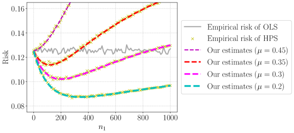
Figure 1: In this figure, we illustrate several intriguing observations. We consider two linear regression tasks and vary the sample size $n_{1}$ of task one and the model shift $\mu$ while fixing the second task. $\mu$ controls the model shift so that $\|\beta^{(1)}-\beta^{(2)}\|^{2}\approx 2\mu^{2}$. For reference, the gray line refers to the empirical excess risk of OLS. Any point above the gray link represents negative transfer, while any point below represents positive transfer. The estimator is defined by solving equation (1.2). In this simulation, we fix feature dimension $p=100$, $n_{2}=300$, and noise variance $\sigma^{2}=1/4$. We give a precise quantification of these transfer effects in Proposition 4.3 below.

We first introduce our problem setup. Let $x_{1}^{(i)},x_{2}^{\mathsf{(}i)},\dots,x_{n_{i}}^{(i)}$ denote feature covariates, where $i$ is either $1$ or $2$. Let $y_{1}^{(i)},y_{2}^{(i)},\dots,y_{n_{i}}^{(i)}$ be their labels. Recall that $n_{1}$ and $n_{2}$ refer to each task’s sample size. We assume a linear model specified by an unknown parameter vector $\beta^{(i)}\in{}^{p}$ as follows:

$$y_{j}^{(i)}=\big{(}x_{j}^{(i)}\big{)}^{\top}{\beta^{(i)}}+\varepsilon_{j}^{(i)},~{}\text{ for any }\ j=1,\dots,n_{i},$$ (1.1)

where $\varepsilon^{(i)}_{j}\in\real$ denotes a random noise variable with mean zero and variance $\sigma^{2}$. For ease of presentation, we refer to the first task as the source and the second task as the target. We assume $n_{2}>p$ while $n_{1}$ can be either less or greater than $p$.

We denote $X^{(1)}\in\mathbb{R}^{n_{1}\times p}$, $X^{(2)}\in\mathbb{R}^{n_{2}\times p}$ as the matrices of covariates, and $Y^{(1)}\in\mathbb{R}^{n_{1}}$, $Y^{(2)}\in\mathbb{R}^{n_{2}}$ are the vectors of labels. Then, we minimize the following objective, parameterized by a shared variable $B\in{}^{p\times r}$:

$$f(B)=\left\|X^{(1)}B-Y^{(1)}\right\|^{2}+\left\|X^{(2)}B-Y^{(2)}\right\|^{2}.$$ (1.2)

Notice that $B$ provides a shared feature space for both tasks. Our results described in the next section will permit straightforward extensions to variants of objective (1.2), including adding weights to each task and adding a ridge penalty. Thus, we will describe our main results for unweighted and unregularized objectives without losing generality. One can see that when $n_{2}>p$, there is a unique minimizer of $f$. We denote this estimator for the target task as $\hat{\beta}_{2}^{\textup{HPS}}$, which is also called hard parameter sharing (HPS) in classical literature (Caruana, 1997). We will evaluate this estimator’s excess risk, denoted by $L(\hat{\beta}_{2}^{\textup{HPS}})$.

Our motivation for studying this simple estimator is that it provides a clean setting to show both positive and negative transfers. In Figure 1, we illustrate three distinct yet intriguing regimes of transfer effects. If the model shift is small, the transfer effect is always positive. If the model shift is moderate, the transfer effect is positive only in a restricted range of values of $n_{1}$. Otherwise, the transfer effect is negative for all $n_{1}$.

A natural variant of the HPS estimator is adding an adjustment $z$ to the source task, which has been used in the estimation procedure of Li et al. (2022). We refer to this as the soft parameter sharing (SPS) estimator, in contrast to the above. Given $\lambda>0$, consider the following optimization objective:

$$f(B,z)=\left\|X^{(1)}(B+z)-Y^{(1)}\right\|^{2}+\left\|X^{(2)}B-Y^{(2)}\right\|^{2}+{\lambda}\left\|z\right\|^{2}.$$ (1.3)

Let $\hat{B},\hat{z}$ denote the minimizer, and the SPS estimator for the target task is defined as $\hat{\beta}_{2}^{\textup{SPS}}(\lambda):=\hat{B}({\lambda})$. $\lambda$ is a regularization parameter that determines the magnitude of $z$. Some techniques we develop will also apply to the SPS estimator.

1.2 Summary of results

We give a summary of our results, which are all in a high-dimensional asymptotic setting, where both $n_{1},n_{2}$ increase to infinity in proportion as $p$ goes to infinity. The results depend on the spectrum of the population covariance matrices of both tasks, denoted as $\Sigma^{(1)}$ and $\Sigma^{(2)}$, which are both $p$ by $p$ matrices. As in the existing random matrix theory literature, let the covariates be given by

$$x_{j}^{(i)}=(\Sigma^{(i)})^{1/2}z_{j}^{(i)},\text{ for any }i=1,2\text{ and }j=1,\dots,n_{i},$$

where $z_{j}^{(i)}$ consists of independent and identically distributed (i.i.d.) entries of mean zero and variance one. Let $X^{(i)}=(x_{1}^{(i)},\ldots,x_{n_{i}}^{(i)})^{\top}\in{}^{n_{i}\times p}$ be the matrix corresponding to the covariates of task $i$. Our goal is to find the asymptotic limit of the excess risk of our estimators on the target task.

Main results.

Deriving the asymptotic limit of our estimators requires studying various functions of two independent sample covariance matrices under covariate shifts. We provide a simplified exposition for $r=1$ and elaborate on the reason in Section 2. First, the variance formula of the excess risk of HPS is equal to

$$\operatorname{Tr}\left[\Sigma^{(2)}\Big{(}{X^{(1)}}^{\top}X^{(1)}+{X^{(2)}}^{\top}X^{(2)}\Big{)}^{-1}\right].$$ (1.4)

The bias formula is more involved and is deferred until Proposition 2.2. The bias and variance both involve the inverse of the sum of both tasks’ sample covariance matrices, which exhibit a covariate shift.

When $n_{2}>p$, the OLS estimator exists, and it is well-known that the limit of its excess risk is equal to ${\frac{\sigma^{2}p}{n_{2}-p}}$ Bai and Silverstein (2010). To the best of our knowledge, the asymptotic limit of the formula (1.4) has not been identified in the literature. Our paper takes the first step to fill the gap. Our results are summarized as follows:

• First, we consider the covariate shift setting, where $\Sigma^{(1)}$ and $\Sigma^{(2)}$ are arbitrary and $\beta^{(1)}=\beta^{(2)}$. In Theorem 3.1, we describe the asymptotic limit of the variance formula as a function of the singular values of the covariate shift matrix. This result generalizes classical results on the limit of the trace of the inverse of one sample covariance matrix to two covariance matrices under covariate shifts.

• Second, we consider the model shift setting, where $\beta^{(1)}$ and $\beta^{(2)}$ are arbitrary and $\Sigma^{(1)}=\Sigma^{(2)}$. In Theorem 4.1, we describe the asymptotic limit of HPS as a function of the Euclidean distance between $\beta^{(1)}$ and $\beta^{(2)}$, and the sample size proportions. Then, in Theorem 4.6, we characterize the bias and variance of the SPS estimator under model shifts and certain technical assumptions.

• Third, we generalize our findings when both the covariate and model shifts are present or when there are multiple source tasks. The detailed results, along with supporting simulations, are provided in length in Theorems 5.1 and 5.2. These results reinforce our results above but apply to more general settings.

Illustrative examples.

We apply the above results to analyze information transfer in a classical random-effects model, where $\beta^{(i)}$ is equal to a shared model vector plus an independent random effect per-task Dobriban and Wager (2018); Fan and Johnstone (2019). The random-effects model provides a natural way to measure the heterogeneity of each task’s model vector.

First, we show that having covariate shifts can either help or hurt performance. We describe an example in Proposition 3.2, showing that when $n_{1}<n_{2}$, transferring from any covariate-shifted data source (i.e., $\Sigma^{(1)}\neq\Sigma^{(2)}$) achieves a lower excess risk of HPS than transferring from the data source with $\Sigma^{(1)}=\Sigma^{(2)}$. On the other hand, when $n_{1}>n_{2}$, transferring from any covariate-shifted data source always incurs a higher excess risk of HPS than transferring from the data source with $\Sigma^{(1)}=\Sigma^{(2)}$.

Second, we identify three information transfer regimes in the random-effects model, explaining the phenomena observed in Figure 1. Let $\mu$ denote the Euclidean distance between $\beta^{(1)}$ and $\beta^{(2)}$. We show the following intriguing regimes:

1. When $\frac{\mu^{2}}{p}\operatorname{Tr}\left[\Sigma^{(1)}\right]\leqslant\frac{\sigma^{2}p}{2(n_{2}-p)}$, the transfer effect is positive for any $n_{1}$: HPS is always better than OLS.

2. When $\frac{\sigma^{2}p}{2(n_{2}-p)}<\frac{\mu^{2}}{p}\operatorname{Tr}\left[\Sigma^{(1)}\right]<\frac{\sigma^{2}n_{2}}{2(n_{2}-p)}$, there exists a deterministic constant $\rho>0$ such that the transfer effect is positive if and only if $n_{1}<\rho p$.

3. When $\frac{\mu^{2}}{p}\operatorname{Tr}\left[\Sigma^{(1)}\right]\geqslant\frac{\sigma^{2}n_{2}}{2(n_{2}-p)}$, the transfer effect is negative for any $n_{1}$: HPS is always worse than OLS.

These examples are not exhaustive, but it is conceivable that the results and techniques may be used to reveal insights about transfer learning further. In particular, we highlight numerous open yet technically-challenging questions along the paper and hope these discussions help inspire further interaction between random matrix theory and learning under dataset shifts.

1.3 Related work

Our work expands on the existing statistical learning literature by contributing a random matrix theory perspective to quantify transfer effects. This differs from early studies that use uniform convergence arguments Baxter (2000); Ben-David and Schuller (2003); Maurer (2006), and the generalization bounds of Crammer et al. (2008); Ben-David et al. (2010a); Wu et al. (2020). The advantage of precise asymptotics compared to generalization bounds is that it allows us to compare the rates of different estimators. This is crucial, as highlighted in Figure 1. There have been several related studies broadly in the space of transfer learning. Li et al. (2022) consider selecting beneficial data sources given multiple sources for transfer learning. The difference between our paper and Li et al. (2022) is that we consider the proportional limit setting. More recently, Duan and Wang (2022) introduces an adaptive and robust estimation procedure when many tasks are present in multitask learning. Wang (2023) studies kernel ridge regression under covariate shifts.

Recent works use random matrix theory to study interpolators in over-parametrized linear/logistic regression (Bartlett et al., 2020; Hastie et al., 2019; Montanari et al., 2019; Liang et al., 2020; Liang and Sur, 2020; Chatterji and Long, 2021) and double-descent (Belkin et al., 2019; Mei and Montanari, 2019). These works deal with covariate matrices in one distribution while we tackle covariances from two distributions. When covariates are sampled from Gaussian distributions, the precise asymptotic limit can be derived directly from the properties of the Wishart distribution. In the high-dimensional setting, the eigenvalues of a Wishart matrix satisfy the well-known Marchenko–Pastur (MP) law (Marčenko and Pastur, 1967), whose Stieltjes transform characterizes the variance limit. Furthermore, it is well-known that the MP law holds universally regardless of the underlying data distribution of the covariates (see, e.g., Bai and Silverstein (2010)). Bloemendal et al. (2014) obtain a sharp convergence rate of the empirical spectral distribution (ESD) to the MP law for sample covariance matrices with isotropic population covariances. Knowles and Yin (2016); Ding and Yang (2018, 2021) later extend this result to sample covariance matrices with arbitrary population covariances. These results are proved by establishing the optimal convergence estimates of the Stieltjes transforms of sample covariance matrices, also known as local laws in the random matrix theory literature. We refer interested readers to Erdos and Yau (2017) and the references for a detailed review of related concepts. One technical contribution of this work is to extend these techniques to the two-task setting and prove an almost sharp local law for the sum of two sample covariance matrices with arbitrary covariate shifts. This local law allows us to derive the precise variance limit depending on the singular values of the covariate shift matrix.

The asymptotic limit of the variance term under covariate shift may also be derived using free probability theory (see, e.g., Nica and Speicher (2006)). However, this approach is not fully justified when the covariates are sampled from non-Gaussian distributions with non-diagonal covariate shift matrices. Furthermore, our result provides almost sharp convergence rates to the asymptotic limit, while it is unclear how to obtain such rates using free probability techniques. The bias term involves asymmetric matrices in terms of two sample covariance matrices, whose analysis is technically involved. Our techniques are inspired by free additions of random matrices (Nica and Speicher, 2006) and recent results (Bao et al., 2017a, b). In particular, we provide the first precise bias limit in the model shift setting, assuming that $\Sigma^{(1)}=\Sigma^{(2)}$ or $\Sigma^{(2)}$ is isotropic, and the covariates are sampled from Gaussian distributions. Showing the asymptotic bias limit under arbitrary covariate and model shifts is an interesting open problem for future work.

Organization.

The rest of this paper is organized as follows. In Section 2, we state the data model and its underlying assumption. Then, we connect the transfer effect of HPS/SPS with their bias-variance decompositions. In Section 3, we present the high-dimensional asymptotic limits of our estimators under covariance shifts. In Section 4, we characterize the high-dimensional asymptotic limits under model shifts. Section 5 extends our findings to more general settings. Lastly, we conclude the paper in Section 6. Appendix A through E fills in missing proofs.

2 Preliminaries

This section sets up the data-generating process that we will work with, along with the underlying assumptions. Then, we connect the transfer effects of the HPS/SPS estimator with a bias-variance decomposition.

2.1 Data

Recall that we have two tasks. For $i=1,2$, $X^{(i)}\in{}^{n_{i}\times p}$ corresponds to task $i$’s covariates and $Y^{(i)}\in{}^{n_{i}}$ corresponds to their labels. Moreover, let $\varepsilon^{(i)}\in{}^{n_{i}}$ be the vector notation corresponding to the additive noise of dataset $i$. Then, equation (1.1) can be reformulated as $Y^{(i)}=X^{(i)}\beta^{(i)}+\varepsilon^{(i)}.$ Assume that $\beta^{(1)}$ and $\beta^{(2)}$ are two arbitrary (deterministic or random) vectors that are independent of $X^{(i)}$ and $\varepsilon^{(i)}$. Throughout the paper, we make the following assumptions on $X^{(i)}$ and $\varepsilon^{(i)}$, which are standard in the random matrix theory literature (see, e.g., Tulino and Verdú (2004); Bai and Silverstein (2010)).

First, the row vectors of $X^{(i)}$ are i.i.d. centered random vectors with $p\times p$ population covariance matrix $\Sigma^{(i)}$ and an $n_{i}\times p$ random matrix $Z^{(i)}=[Z^{(i)}_{jk}]$ with independent entries of zero mean and unit variance:

$$X^{(i)}=Z^{(i)}(\Sigma^{(i)})^{1/2}\in{}^{n_{i}\times p}.$$ (2.1)

Let $\tau>0$ be a small constant. Suppose the $\varphi$-th moment of each entry $Z^{(i)}_{jk}$ is bounded from above by $1/\tau$, for a constant $\varphi>4$:

$$\mathop{\mathbb{E}}\left[\big{|}Z^{(i)}_{jk}\big{|}^{\varphi}\right]\leqslant{\tau}^{-1}.$$ (2.2)

The eigenvalues of $\Sigma^{(i)}$, denoted as $\sigma^{(i)}_{1},\cdots,\sigma^{(i)}_{p}$, are all bounded between $\tau$ and $\tau^{-1}$:

$$\tau\leqslant\sigma^{(i)}_{p}\leqslant\cdots\leqslant\sigma^{(i)}_{2}\leqslant\sigma^{(i)}_{1}\leqslant\tau^{-1}.$$ (2.3)

Second, $\varepsilon^{(i)}\in{}^{n_{i}}$ is a random vector with independent entries having mean zero, variance $\sigma^{2}$, and bounded moments up to any order, i.e., for any fixed $k\in\mathbb{N}$, there exists a constant $C_{k}>0$ such that

$$\mathop{\mathbb{E}}\left[\big{|}{\varepsilon}^{(i)}_{j}\big{|}^{k}\right]\leqslant C_{k}.$$ (2.4)

Third, the sample sizes are comparable to the dimension $p$. Denote by $\rho_{1}=n_{1}/p$ and $\rho_{2}=n_{2}/p$. Assume

$$0\leqslant\rho_{1}\leqslant p^{\tau^{-1}},\quad 1+\tau\leqslant\rho_{2}\leqslant p^{\tau^{-1}},\quad 0\leqslant{\rho_{1}}/{\rho_{2}}\leqslant\tau^{-1}.$$ (2.5)

The condition $\rho_{2}\geqslant 1+\tau$ ensures that the target task’s sample covariance matrix is full rank with high probability. The upper bound $\rho_{i}\leqslant p^{\tau^{-1}}$ is a mild condition; otherwise, standard concentration results such as the central limit theorem already give accurate estimates in the linear model. The condition ${\rho_{1}}/{\rho_{2}}\leqslant\tau^{-1}$ ensures the sample size imbalance between the two tasks is bounded by a factor that does not grow with $p$. To summarize, the underlying assumptions of the data model are as follows.

Assumption 2.1 (Data generating model).

Let $\tau>0$ be a small constant. ($X^{(1)},X^{(2)},\varepsilon^{(1)},\varepsilon^{(2)}$) are mutually independent. Moreover, the followings hold for any $i=1,2$:

1. $X^{(i)}$ takes the form (2.1), where $Z^{(i)}$ is a random matrix with i.i.d. entries having zero mean, unit variance, and bounded moments as in equation (2.2), and $\Sigma^{(i)}$ is a deterministic positive definite symmetric matrix satisfying (2.3).

2. $\varepsilon^{(i)}\in{}^{n}$ is a random vector consisting of i.i.d. entries of zero mean, variance $\sigma^{2}$, and bounded moments as in equation (2.4).

3. $\rho_{i}$ satisfies equation (2.5).

2.2 Risks

The risk of $\hat{\beta}_{i}^{\textup{HPS}}$ over an unseen sample $(x,y)$ of the target task $i$ is given by (under the mean squared loss):

$$\mathop{\mathbb{E}}_{x,\varepsilon}\left[\left\|y-x^{\top}\hat{\beta}_{i}^{\textup{HPS}}\right\|^{2}\right]=\left\|{\Sigma^{(i)}}^{1/2}\left(\hat{\beta}_{i}^{\textup{HPS}}-\beta^{(i)}\right)\right\|^{2}+\sigma^{2}.$$

The excess risk is the difference between the above risk and the expected risk of the population risk optimizer:

$$L(\hat{\beta}_{i}^{\textup{HPS}}):=\left\|{\Sigma^{(i)}}^{1/2}\left(\hat{\beta}_{i}^{\textup{HPS}}-\beta^{(i)}\right)\right\|^{2}.$$ (2.6)

We focus on a setting with $r=1$ (recall that $r$ is the width of the network’s hidden layer) and take $i=2$ as the target task. The target task’s OLS estimator is $\hat{\beta}_{2}^{\textup{OLS}}=\big{(}{X^{(2)}}^{\top}X^{(2)}\big{)}^{-1}{X^{(2)}}^{\top}Y^{(2)}$, which is well-defined given Assumption 2.1. When $r\geqslant 2$, it is shown that (Wu et al., 2020) the HPS estimator reduces to OLS.

Next, we present a bias-variance decomposition of the excess risk of HPS. Several notations are needed to present the result. Denote the sum of both tasks’ sample covariance matrix as:

$$\hat{\Sigma}={X^{(1)}}^{\top}X^{(1)}+{X^{(2)}}^{\top}X^{(2)}.$$ (2.7)

The next result provides the bias and variance formulas for the excess risk of the HPS estimator.

Lemma 2.2 (Bias-variance of HPS).

Under Assumption 2.1, for any small constant ${\mathit{c}}>0$, with high probability over the randomness of the training samples ($X^{(1)},Y^{(1)},X^{(2)},Y^{(2)}$), the following estimates hold:

$$L(\hat{\beta}_{2}^{\textup{HPS}})= \left[1+\operatorname{O}(p^{-1/2+c})\right]\cdot\left(L_{\text{bias}}+L_{\text{var}}\right),$$ (2.8)

where the bias and variance formulas are defined as

$$L_{\text{bias}} =\left\|{\Sigma^{(2)}}^{1/2}\hat{\Sigma}^{-1}\big{(}{{X^{(1)}}^{\top}X^{(1)}}\big{)}\big{(}\beta^{(1)}-\beta^{(2)}\big{)}\right\|^{2},$$ (2.9)

$$L_{\text{var}} =\sigma^{2}\operatorname{Tr}\big{(}{\Sigma^{(2)}\hat{\Sigma}^{-1}}\big{)}.$$ (2.10)

Hereafter, an event $\Xi$ is said to hold with high probability (w.h.p.) if $\mathbb{P}(\Xi)\to 1$ as $p\to\infty$. Moreover, the big-$\operatorname{O}$ notation $A=\operatorname{O}(B)$ means that $|A|\leqslant C|B|$ for a constant $C>0$ depending on the model parameters in Section 2.1 (i.e., $\tau$, $\varphi$ and $C_{k}$’s), but not on $p$, $n_{1}$ and $n_{2}$. Hence, the equation (2.8) holds w.h.p. can be equivalently stated as

$$\lim_{p\to\infty}\mathbb{P}\left(\left|L(\hat{\beta}_{2}^{\textup{HPS}})-L_{\text{bias}}-L_{\text{var}}\right|\leqslant Cp^{-1/2+c}(L_{\text{bias}}+L_{\text{var}})\right)=1$$

for a constant $C>0$. The proof of Lemma 2.2 can be found in Appendix B.

While the formulas may seem tedious, they allow us to reason about transfer effects by comparing the bias and variance of HPS with that of OLS. Notice that the bias of OLS is zero since $n_{2}\geqslant(1+\tau)p$ under Assumption 2.1. Hence, the bias of HPS is always larger than that of OLS. On the other hand, the variance of HPS is always lower than that of OLS. Let $X^{(1)}=0$ in equation (2.10). By Woodbury matrix identity, the variance of OLS is always higher than formula (2.10):

$$\operatorname{Tr}\left[\Sigma^{(2)}\big{(}{X^{(2)}}^{\top}X^{(2)}\big{)}^{-1}\right]\geqslant\operatorname{Tr}\left[\Sigma^{(2)}{\hat{\Sigma}}^{-1}\right],$$ (2.11)

Thus, the transfer effect of HPS is determined by the bias-variance decomposition: the bias always increases while the variance always decreases. Whether or not the transfer effect of HPS is positive depends on which effect dominates. Similar observations will also apply to SPS.

The above discussion highlights the need for precise bias-variance estimates to determine transfer effects. However, finding the exact limits is challenging because of dataset shifts. Moreover, these shifts manifest in various forms. To make progress in this important yet challenging problem, we divide our study according to various combinations of covariate and model shifts:

• Section 3 is devoted to the precise estimate of $L_{\text{var}}$ for the HPS estimator under an arbitrary covariate shift but no model shift.

• Section 4 studies the effect of model shifts: Section 4.1 and Section 4.2 give precise estimates of $L_{\text{bias}}$ and $L_{\text{var}}$ for the HPS estimator and SPS estimator, respectively.

• Section 5 extends these results to a classical setting of the random-effects model with both covariate and model shifts, and a setting with multiple source tasks.

3 Estimates under Covariate Shifts

This section presents a precise estimate of $L_{\text{var}}$ in (2.10) with an almost sharp convergence rate for the HPS estimator under arbitrary covariate shift. Then, we will discuss some interesting implications of this result regarding the impact of covariate shifts on transfer effects. Simulations demonstrate that the exact asymptotics are remarkably accurate even when $p$ is only $50$.

3.1 Sample covariance matrices with covariate shifts

Suppose the two tasks satisfy the same linear model ($\beta^{(1)}=\beta^{(2)}$) but have different population covariance matrices ($\Sigma^{(1)}\neq\Sigma^{(2)}$). Recall that the matrix $\hat{\Sigma}$ in equation (2.7) is a sum of two sample covariance matrices. Thus, the expectation of $\hat{\Sigma}$ is equal to a mixture of $\Sigma^{(1)}$ and $\Sigma^{(2)}$, with mixing proportions determined by the sample sizes $n_{1}$ and $n_{2}$. Intuitively, the spectrum of $\hat{\Sigma}^{-1}$ not only depends on $n_{1},n_{2}$, but also depends on how well aligned $\Sigma^{(1)}$ and $\Sigma^{(2)}$ are. To capture this alignment, we introduce the covariate shift matrix $M:={\Sigma^{(1)}}^{1/2}{\Sigma^{(2)}}^{-1/2}$. Let $\lambda_{1}\geqslant\lambda_{2}\geqslant\dots\geqslant\lambda_{p}$ be the singular values of $M$ in descending order. Our first main result is the following theorem on the variance limit, which characterizes the exact dependence of $L_{\text{var}}$ on the singular values of $M$ and the sample sizes $n_{1}$, $n_{2}$.

Theorem 3.1 (Exact estimates under covariate shifts).

Under Assumption 2.1, for any small constant $c>0$, with high probability over the randomness of $(X^{(1)},X^{(2)})$, the following holds:

$${\left|{L_{\text{var}}-\frac{\sigma^{2}}{n_{1}+n_{2}}\operatorname{Tr}\left[\Big{(}{\alpha_{1}M^{\top}M+\alpha_{2}\operatorname{Id}_{p\times p}}\Big{)}^{-1}\right]}\right|}\leqslant\sigma^{2}p^{1/2}(n_{1}+n_{2})^{\frac{2}{\varphi}-\frac{3}{2}+c},$$ (3.1)

where $\alpha_{1}$ and $\alpha_{2}$ are the unique positive solutions of the following system of equations:

$$\alpha_{1}+\alpha_{2}=1-\frac{p}{n_{1}+n_{2}},\quad\alpha_{1}+\frac{1}{n_{1}+n_{2}}\sum_{i=1}^{p}\frac{\lambda_{i}^{2}\alpha_{1}}{\lambda_{i}^{2}\alpha_{1}+\alpha_{2}}=\frac{n_{1}}{n_{1}+n_{2}}.$$ (3.2)

Recalling that $\varphi>4$, for a small enough constant $c$, equation (3.1) characterizes the limit of $L_{var}$ with an error term that is smaller than the deterministic leading term by a factor $\operatorname{o}({p}^{-1/2})$.

Theorem 3.1 generalizes a classical result in multivariate statistics to the sum of two independent sample covariance matrices with arbitrary covariate shift: with high probability over the randomness of $X^{(2)}$,

$$\operatorname{Tr}\left[\Sigma^{(2)}\big{(}{{X^{(2)}}^{\top}X^{(2)}}\big{)}^{-1}\right]=\frac{p}{n_{2}-p}+\operatorname{O}\left(p^{1/2}n^{\frac{2}{\varphi}-\frac{3}{2}+c}\right).$$ (3.3)

To see this, note that (3.3) is a special case of Theorem 3.1 with $n_{1}=0$. For this case, equation (3.2) implies that $\alpha_{1}=0$ and $\alpha_{2}=(n_{2}-p)/{n_{2}}.$ Therefore,

$$\frac{1}{n_{1}+n_{2}}\operatorname{Tr}\left[\Big{(}{\alpha_{1}M^{\top}M+\alpha_{2}\operatorname{Id}_{p\times p}}\Big{)}^{-1}\right]=\frac{p}{n_{2}-p}.$$ (3.4)

The result (3.3) has a rich history in the random matrix theory literature. When $Z^{(2)}$ is a Gaussian random matrix, the limit (without a convergence rate) follows from properties of the inverse Wishart distribution (Anderson, 2003). Otherwise, one can use the Stieltjes transform method to derive the estimate (Lemma 3.11, Bai and Silverstein (2010)). The estimate (3.3) with sharp convergence rates can be found in Theorem 2.4 Bloemendal et al. (2014) and Theorem 3.14 Ding and Yang (2018).

Theorem 3.1 follows from a sharp local law on the resolvent of $\hat{\Sigma}$, which we will establish based on some recent developments in random matrix theory (Knowles and Yin, 2016; Yang, 2019). For more details, we refer the reader to Appendix C.2.

3.2 Illustrating the effects of covariate shift on transfer

Next, we provide two illustrative examples of Theorem 3.1, based on which we revisit the impact of covariate shift upon transfer. Notice that in the case where both tasks enjoy the same linear model ($\beta^{(1)}=\beta^{(2)}$), HPS always incurs a lower risk than OLS. Therefore, the comparison will be between HPS estimators under different degrees of covariate shifts.

In the first example, we show that the impact of covariate shift indeed depends on the ratio between $n_{1}$ and $n_{2}$. While covariate shift is often considered a detriment in empirical research, we demonstrate that it may help in certain cases. Let $p$ be an even integer and $g(M)=\frac{\sigma^{2}}{n_{1}+n_{2}}\operatorname{Tr}\left[(\alpha_{1}M^{\top}M+\alpha_{2}\operatorname{Id}_{p\times p})^{-1}\right]$. We compare $g(M)$ for different $M$ within a set $\mathcal{S}$ such that $\lambda_{p+1-i}=1/{\lambda_{i}}$ for $i=1,2,\dots,p/2$. Therefore, every matrix in $\mathcal{S}$ is normalized with $\det(M)=1$. In particular, $M=\operatorname{Id}_{p\times p}$ represents two tasks with the same population covariance matrix. We show that when $n_{1}<n_{2}$, having covariate shifts is better for HPS, but when $n_{1}>n_{2}$, covariate shifts are detrimental.

Proposition 3.2 (Effect of covariate shift, I).

Within the set $M\in\mathcal{S}$, the following dichotomy regarding $g(\operatorname{Id}_{p\times p})$ and $g(M)$ holds:

1. When $n_{1}<n_{2}$, $g(M)\leqslant g(\operatorname{Id}_{p\times p})$ for any $M\in\mathcal{S}$.

2. When $n_{1}\geqslant n_{2}$, $g(\operatorname{Id}_{p\times p})\leqslant g(M)$ for any $M\in\mathcal{S}$.

Proof.

By definition, we can expand $g(M)$ as

$$g(M)=\frac{\sigma^{2}}{n_{1}+n_{2}}\sum_{i=1}^{p/2}\left(\frac{1}{\lambda_{i}^{2}\alpha_{1}+\alpha_{2}}+\frac{1}{\lambda_{i}^{-2}\alpha_{1}+\alpha_{2}}\right).$$

When $M=\operatorname{Id}_{p\times p}$, we have $g(\operatorname{Id}_{p\times p})=\frac{\sigma^{2}p}{n_{1}+n_{2}-p},$ which can also be written as $\frac{\sigma^{2}}{n_{1}+n_{2}}\sum_{i=1}^{p/2}\frac{2}{\alpha_{1}+\alpha_{2}}$, since $\alpha_{1}+\alpha_{2}=1-\frac{p}{n_{1}+n_{2}}$ by (3.2). Then, we subtract $g(\operatorname{Id}_{p\times p})$ from $g(M)$ to get

$$g(M)-g(\operatorname{Id}_{p\times p}) =\frac{\sigma^{2}}{n_{1}+n_{2}-p}\sum_{i=1}^{p/2}\frac{(\lambda_{i}^{2}-1)^{2}\alpha_{1}\left(\alpha_{1}-\alpha_{2}\right)}{(\alpha_{1}+\lambda_{i}^{2}\alpha_{2})(\lambda_{i}^{2}\alpha_{1}+\alpha_{2})}.$$

We claim that $\alpha_{1}>\alpha_{2}$ if and only if $n_{1}>n_{2}$, thus proving the dichotomy. When $\alpha_{1}>\alpha_{2}$, the first part of equation (3.2) implies $\alpha_{1}>\frac{1}{2}(1-\frac{p}{n_{1}+n_{2}})$. The second part of equation (3.2) gives

$$\frac{n_{1}}{n_{1}+n_{2}} =\alpha_{1}+\frac{1}{n_{1}+n_{2}}\sum_{i=1}^{p}\frac{\lambda_{i}^{2}\alpha_{1}}{\lambda_{i}^{2}\alpha_{1}+\alpha_{2}}$$

$$>\frac{1}{2}\Big{(}1-\frac{p}{n_{1}+n_{2}}\Big{)}+\frac{1}{n_{1}+n_{2}}\sum_{i=1}^{p/2}\left(\frac{\lambda_{i}^{2}}{\lambda_{i}^{2}+1}+\frac{\lambda_{i}^{-2}}{\lambda_{i}^{-2}+1}\right)$$

$$=\frac{1}{2}\Big{(}1-\frac{p}{n_{1}+n_{2}}\Big{)}+\frac{p}{2(n_{1}+n_{2})}=\frac{1}{2},$$

implying $n_{1}>n_{2}$. When $\alpha_{1}<\alpha_{2}$, one can show $n_{1}<n_{2}$ using similar steps. This completes the proof. ∎

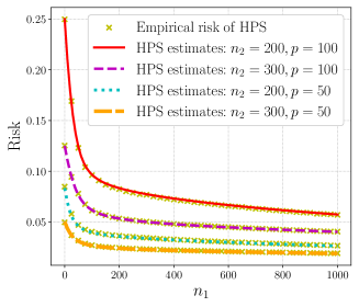
((a)) Varying $n_{2}$ and $p$

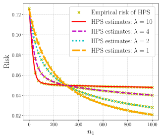
((b)) Varying covariate shift $\lambda$

Figure 2: Illustration of Theorem 3.1 under various sample sizes and dimensions. Figure 2(a) shows that the variance estimate accurately matches the empirical risks. This simulation fixes $\lambda=4$ and varies $n_{1},n_{2},p$. Figure 2(b) shows the dichotomy in Proposition 3.2. When $n_{1}<n_{2}$, the lowest risk is achieved by transferring from a covariate-shifted dataset. When $n_{1}\geqslant n_{2}$, the lowest risk is achieved by transferring from a dataset with $\Sigma^{(1)}=\Sigma^{(2)}$. This simulation fixes $p=100,n_{2}=300$ and varies $n_{1},\lambda$. Both simulations use $\sigma=1/2$.

Figure 2 illustrates a special case where $\lambda_{1}=\cdots=\lambda_{{p/2}}=\lambda>1$ and $\lambda_{{p/2}+1}=\cdots=\lambda_{p}=1/\lambda$. Thus, higher $\lambda$ corresponds to a worse covariate shift. We plot the theoretical estimate using $g(M)$ and the excess risk using equation (2.10). We observe that our theoretical estimate in Theorem 3.1 matches the empirical risk incredibly well. As a result, we indeed observe the dichotomy in Proposition 3.2. Furthermore, for larger $\lambda$, the excess risk of HPS decreases slower, indicating a worse “rate of transfer” from task one. As a remark, impossibility results for transfer learning under covariate shift have been observed for classification (Ben-David et al., 2010b); our results show this in high-dimensional regression.

In the second example, we further study the case of $n_{1}\geqslant n_{2}$. A common scenario in transfer learning is that the source dataset is much larger than the target dataset. We show that when $n_{1}$ is greater than $n_{2}$ times a sufficiently large constant, $M=\operatorname{Id}_{p\times p}$ indeed minimizes $g(M)$ within a bounded set of matrices whose determinants are equal to one. The proof of the following result can be found in Section C.1.

Proposition 3.3 (Effect of covariate shift, II).

Let $c\in(0,1)$ be a fixed constant. Let $\mathcal{S}^{\prime}$ be a set of matrices such that for any $M\in\mathcal{S}^{\prime}$: (i) $\det(M)=1$; (ii) the eigenvalues $\lambda_{1}^{2},\ldots,\lambda_{p}^{2}$ of $M^{\top}M$ are bounded between $c$ and $1/c$. If $n_{1}-p\geqslant c^{-1}n_{2}$, then $g$ achieves the global minimum at $\operatorname{Id}_{p\times p}$, i.e.,

$$g(\operatorname{Id}_{p\times p})\leqslant g(M),~{}\text{for any}~{}M\in\mathcal{S}^{\prime}.$$ (3.5)

We remark that (3.5) may not hold if we do not assume that the eigenvalues $\lambda_{1}^{2},\ldots,\lambda_{p}^{2}$ are bounded. For example, choose $M=M_{x}$ with $\lambda_{p}^{2}=x>1$ and $\lambda_{1}^{2}=\cdots=\lambda_{p-1}^{2}=x^{-(p-1)^{-1}}$. Let $(\alpha_{1}(x),\alpha_{2}(x))$ be the solution to the system of equations

$$\alpha_{1}+\alpha_{2}=1-\frac{p}{n_{1}+n_{2}},\quad\alpha_{1}+\frac{1}{n_{1}+n_{2}}\left(\frac{(p-1)x^{-(p-1)^{-1}}\alpha_{1}}{x^{-(p-1)^{-1}}\alpha_{1}+\alpha_{2}}+\frac{x\alpha_{1}}{x\alpha_{1}+\alpha_{2}}\right)=\frac{n_{1}}{n_{1}+n_{2}}.$$ (3.6)

From this equation, we obtain that $\alpha_{1}(x)\to\frac{n_{1}-1}{n_{1}+n_{2}}$ and $\alpha_{1}(x)\to\frac{n_{2}+1-p}{n_{1}+n_{2}}$ as $x\to\infty$. Thus,

$$\lim_{x\to\infty}g(M_{x}) =\lim_{x\to\infty}\frac{\sigma^{2}}{n_{1}+n_{2}}\left(\frac{p-1}{x^{-(p-1)^{-1}}\alpha_{1}(x)+\alpha_{2}(x)}+\frac{1}{x\alpha_{1}(x)+\alpha_{2}(x)}\right)$$

$$=\frac{\sigma^{2}(p-1)}{n_{2}+1-p}\geqslant\frac{\sigma^{2}p}{n_{1}+n_{2}-p}=g(\operatorname{Id}_{p\times p}).$$

Similar arguments, by comparing $g(\operatorname{Id}_{p\times p})$ with $g(M)$ for certain $M$ on the boundary of $\mathcal{S}^{\prime}$, show that $(n_{1}-p)/n_{2}$ should have a proper lower bound in order for $g(\operatorname{Id}_{p\times p})$ to be the global minimum. We use an induction argument in Section C.1 to show that $(n_{1}-p)/n_{2}\geqslant c^{-1}$ is a sufficient condition.

3.3 Numerical comparisons

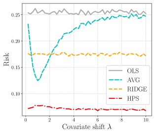
Figure 3: Comparing the excess prediction risks of HPS, OLS, RIDGE, and AVG (lower is better). For reference, this simulation uses $p=50,n_{1}=n_{2}=100,$ and $\sigma=1/2$.

We show that the HPS estimator enjoys superior empirical performance compared to several other natural transfer learning estimators. For this comparative study, we include the OLS estimator and the ridge estimator (RIDGE):

$$\hat{\beta}_{2}^{\textup{RIDGE}}(k)=\big{(}{X^{(2)}}^{\top}X^{(2)}+k\cdot\operatorname{Id}_{p\times p}\big{)}^{-1}{X^{(2)}}^{\top}Y^{(2)}.$$

We also consider an averaging estimator (AVG), which takes a convex combination of their OLS estimators:

$$\hat{\beta}_{2}^{\text{AVG}}(b)=b\cdot\hat{\beta}^{\textup{OLS}}_{1}+(1-b)\cdot\hat{\beta}^{\textup{OLS}}_{2}.$$

The parameters $b$ and $k$ are optimized using a validation set independent of the training set. For HPS, a weight parameter for each task and a ridge penalty are added. These are both optimized using the validation set. We remark that all the high-dimensional asymptotic limits for HPS can be extended to this setting. As shown in Figure 3, we find that HPS consistently outperforms OLS, RIDGE, and AVG in this simulation.

4 Estimates under Model Shifts

This section presents precise estimates of the bias and variance formulas for the HPS/SPS estimator under model shifts when there is no covariate shift. With these results, we can connect the bias-variance decomposition to transfer effects by comparing the bias and variance of HPS/SPS with those of OLS. In particular, we will present a detailed theoretical analysis of information transfer in the classical random-effect model. We also provide simulations to justify the validity of the asymptotics for finite $p$.

4.1 The HPS estimator

In this subsection, we study the impact of model shifts on the performance of the HPS estimator when there is no covariate shift. Particularly, both tasks have the same population covariance matrix ($\Sigma^{(1)}=\Sigma^{(2)}$) but follow different linear models ($\beta^{(1)}\neq\beta^{(2)}$). The following result states the exact asymptotic limit of the excess risk of HPS in this case.

Theorem 4.1 (Exact estimates under model shifts).

Under Assumption 2.1, suppose that $\Sigma^{(1)}=\Sigma^{(2)}$ and $Z^{(1)}$ and $Z^{(2)}$ are both Gaussian random matrices. Then, for any small constant ${\mathit{c}}>0$, with high probability over the randomness of $(Z^{(1)},Z^{(2)})$, the following estimates hold:

$$L_{var} =\sigma^{2}L_{1}+\operatorname{O}\big{(}\sigma^{2}p^{1/2}{(n_{1}+n_{2})^{-3/2+c}}{}\big{)},$$ (4.1)

$$L_{bias} =\left\|{\Sigma^{(1)}}^{1/2}\big{(}\beta^{(1)}-\beta^{(2)}\big{)}\right\|^{2}L_{2}+\operatorname{O}\left(p^{-1/2+c}\left\|\beta^{(1)}-\beta^{(2)}\right\|^{2}\right).$$ (4.2)

Above, $L_{1}$ and $L_{2}$ are defined as

$$L_{1} =\frac{p}{n_{1}+n_{2}-p},\quad L_{2}=\frac{n_{1}^{2}(n_{1}+n_{2}-p)+pn_{1}n_{2}}{(n_{1}+n_{2})^{2}(n_{1}+n_{2}-p)}.$$

Combining equations Theorem 4.1 with Lemma 2.2 results in an exact estimate for the excess risk of HPS under model shifts. The variance estimate (4.1) is a special case of Theorem 3.1 with $M=\operatorname{Id}_{p\times p}$ and $\varphi\to\infty$ (since Gaussian random variables have bounded moments up to any order).

The bias estimate (4.2) requires the assumption that both $Z^{(1)}$ and $Z^{(2)}$ are Gaussian. We briefly describe the proof ideas. Let $\operatorname{\mathbf{v}}=(\Sigma^{(1)})^{1/2}\left(\beta^{(1)}-\beta^{(2)}\right)$. Then, the bias formula (2.9) can be written as:

$$L_{bias} =\operatorname{\mathbf{v}}^{\top}{Z^{(1)}}^{\top}Z^{(1)}{\left({Z^{(1)}}^{\top}Z^{(1)}+{Z^{(2)}}^{\top}Z^{(2)}\right)^{-2}}{Z^{(1)}}^{\top}Z^{(1)}\operatorname{\mathbf{v}}.$$

Since both $Z^{(1)}$ and $Z^{(2)}$ are Gaussian random matrices, the distributions of ${Z^{(1)}}^{\top}Z^{(1)}$ and ${Z^{(2)}}^{\top}Z^{(2)}$ are rotation-invariant. Thus, the following (approximate) identity holds up to a small error:

$$L_{bias} \approx\frac{\|\operatorname{\mathbf{v}}\|^{2}}{p}\operatorname{Tr}\left[\big{(}{Z^{(1)}}^{\top}Z^{(1)}\big{)}^{2}{\left({Z^{(1)}}^{\top}Z^{(1)}+{Z^{(2)}}^{\top}Z^{(2)}\right)^{-2}}\right]$$

$$=\frac{\|\operatorname{\mathbf{v}}\|^{2}}{p}\left.\frac{\mathrm{d}}{\mathrm{d}x}\right|_{x=0}\operatorname{Tr}\left[\Big{(}{Z^{(1)}}^{\top}Z^{(1)}+x\big{(}{Z^{(1)}}^{\top}Z^{(1)}\big{)}^{2}+{Z^{(2)}}^{\top}Z^{(2)}\Big{)}^{-1}\right].$$ (4.3)

Due to the rotation invariance, the asymptotic limit of equation (4.3) is determined by the free addition of ${Z^{(1)}}^{\top}Z^{(1)}+x({Z^{(1)}}^{\top}Z^{(1)})^{2}$ and ${Z^{(2)}}^{\top}Z^{(2)}$. Building on free probability techniques (see e.g., Nica and Speicher (2006); Bao et al. (2017a, b)), an explicit formula for this free addition can be derived for any $x$ around zero. This observation allows one to derive equation (4.2) by taking the derivative with respect to $x$ as in equation (4.3). More details including the complete proof of Theorem 4.1 are presented in Appendix D.1.

Remark 4.2.

We conjecture that the bias limit (4.2) is still the exact asymptotic form even if $Z^{(1)}$ and $Z^{(2)}$ are non-Gaussian random matrices. One approach to show this is using the local laws for polynomials of random matrices Erdős et al. (2020). This requires checking certain technical regularity conditions, which is an interesting question for future work.

4.1.1 Examples

We will consider a random-effects model, building on existing works (Dobriban and Wager, 2018; Dobriban and Sheng, 2020). Each $\beta^{(i)}$ consists of two components in this case, one shared by all tasks and one that is task-specific. Let $\beta_{0}$ be the shared component and $\gamma_{i}$ be the $i$-th task-specific component. For any $i$, the $i$-th model vector is equal to $\beta^{(i)}=\beta_{0}+\gamma_{i}.$ The entries of the task-specific component $\gamma_{i}$ are drawn independently from a Gaussian distribution with mean zero and variance $p^{-1}\mu^{2}$, for a parameter $\mu>0$. In expectation, the Euclidean distance between the two model vectors is equal to $2\mu^{2}$.

Based on Theorem 4.1, we present a precise analysis of information transfer in this random-effects model using the precise limits in Theorem 4.1.

Proposition 4.3 (Effect of model shift).

Under the assumptions of Theorem 4.1, suppose the random-effect model applies and $n_{2}\geqslant 3p$. Let $a={p}^{-1}\operatorname{Tr}\left[\Sigma^{(1)}\right]$. For any small constant $c>0$, the following statements hold with high probability over the randomness of training samples and model vectors.

1. If ${\mu^{2}}a\leqslant\frac{\sigma^{2}p}{2(n_{2}-p)}$, then the transfer effect is positive:

   $$L(\hat{\beta}_{2}^{\textup{HPS}})\leqslant\left(1+\operatorname{O}(p^{-1/2+c})\right)\cdot L(\hat{\beta}_{2}^{\textup{OLS}}).$$ (4.4)

2. If $\frac{\sigma^{2}p}{2(n_{2}-p)}<{\mu^{2}}a<\frac{\sigma^{2}n_{2}}{2(n_{2}-p)}$, then there exists a deterministic value $n_{0}>0$ (which may not be an integer) such that if $n_{1}\leqslant n_{0}$, then case (4.4) holds; otherwise if $n_{1}>n_{0}$, the other case holds:

   $$L(\hat{\beta}_{2}^{\textup{OLS}})\leqslant\left(1+\operatorname{O}(p^{-1/2+c})\right)\cdot L(\hat{\beta}_{2}^{\textup{HPS}}).$$ (4.5)

3. If ${\mu^{2}}a\geqslant\frac{\sigma^{2}n_{2}}{2(n_{2}-p)}$, then case (4.5) holds for any $n_{1}>p$.

Proof.

Since $\|(\Sigma^{(1)})^{1/2}\left(\beta^{(1)}-\beta^{(2)}\right)\|^{2}=(2+\operatorname{O}(p^{-1/2+c})){\mu^{2}}a$ with high probability, the limit of $L(\hat{\beta}_{2}^{\textup{HPS}})$ is equal to

$$\ell(n_{1}):=\sigma^{2}L_{1}+2\mu^{2}aL_{2}=\frac{\sigma^{2}p}{n_{1}+n_{2}-p}+2{\mu^{2}}a\cdot\frac{n_{1}^{2}(n_{1}+n_{2}-p)+pn_{1}n_{2}}{(n_{1}+n_{2})^{2}(n_{1}+n_{2}-p)}.$$ (4.6)

By Theorem 4.1, we have that with high probability,

$$L(\hat{\beta}_{2}^{\textup{HPS}})=\left(1+\operatorname{O}(p^{-1/2+c})\right)\cdot\ell(n_{1}).$$ (4.7)

By equation (3.3), with high probability over the randomness of $X^{(2)}$, the excess risk of the OLS estimator is

$$L(\hat{\beta}_{2}^{\textup{OLS}})=\sigma^{2}\cdot\operatorname{Tr}\left[\Sigma^{(2)}\big{(}{X^{(2)}}^{\top}X^{(2)}\big{)}^{-1}\right]=\left(1+\operatorname{O}(p^{-1+c})\right)\cdot\frac{\sigma^{2}p}{n_{2}-p}.$$ (4.8)

Thus, whether or not $L(\hat{\beta}_{2}^{\textup{HPS}})\leqslant L(\hat{\beta}_{2}^{\textup{OLS}})$ reduces to comparing $\ell(n_{1})$ and $\frac{\sigma^{2}p}{n_{2}-p}$. Let $h(n_{1})$ be their difference:

$$h(n_{1})=2\mu^{2}a\cdot\frac{n_{1}^{2}(n_{1}+n_{2}-p)+pn_{1}n_{2}}{(n_{1}+n_{2})^{2}(n_{1}+n_{2}-p)}-\frac{\sigma^{2}pn_{1}}{(n_{1}+n_{2}-p)(n_{2}-p)}.$$

The sign of $h(n_{1})$ is the same as the sign of the following second-order polynomial in $n_{1}$:

$$\tilde{h}(n_{1}) =2\mu^{2}a(n_{2}-p)(n_{1}(n_{1}+n_{2}-p)+pn_{2})-\sigma^{2}p(n_{1}+n_{2})^{2}$$

$$=\big{(}2\mu^{2}a(n_{2}-p)-\sigma^{2}p\big{)}n_{1}^{2}+(2\mu^{2}a(n_{2}-p)^{2}-2\sigma^{2}pn_{2})n_{1}+\big{(}2\mu^{2}a(n_{2}-p)pn_{2}-\sigma^{2}pn_{2}^{2}\big{)}.$$

Let $C_{0},C_{1},C_{2}$ be the coefficients of $n_{1}^{0},n_{1}^{1},n_{1}^{2}$ terms in $\tilde{h}(n_{1})$. We prove each claim as follows.

1. If $\mu^{2}a\leqslant\frac{\sigma^{2}p}{2(n_{2}-p)}$, then $C_{0},C_{1},C_{2}$ are all non-positive, which gives $\tilde{h}(n_{1})\leqslant 0$.

2. If $\frac{\sigma^{2}p}{2(n_{2}-p)}<\mu^{2}a<\frac{\sigma^{2}n_{2}}{2(n_{2}-p)}$, then $C_{2}>0$ and $C_{0}<0$. Thus, $\tilde{h}(n_{1})$ has a positive root and a negative root. Let the positive root of $\tilde{h}(n_{1})$ be $n_{0}\in\mathbb{R}$. Then, $\tilde{h}(n_{1})\leqslant 0$ if $n_{1}\leqslant n_{0}$, and $\tilde{h}(n_{1})\geqslant 0$ otherwise.

3. If $\mu^{2}a\geqslant\frac{\sigma^{2}n_{2}}{2(n_{2}-p)}$, then $C_{0}$ and $C_{2}$ are both non-negative. Furthermore, we can check that $C_{1}\geqslant 0$ using the assumption $n_{2}\geqslant 3p$. Hence, we have $\tilde{h}(n_{1})\geqslant 0$ for all $n_{1}$.

Combining these three cases with equations (4.7) and (4.8) concludes the proof. ∎

Figure 1 illustrates Proposition 4.3 for multiple values of $\mu$. We plot the theoretical estimate using $\ell(n_{1})$ and the excess risk using the sum of equations (2.9) and (2.10). This simulation shows that our estimate accurately matches the empirical risks. Additionally, the three information transfer regimes are also observed by varying $\mu$ in the random-effect model. This simulation sets $\Sigma^{(1)}=\Sigma^{(2)}=\operatorname{Id}_{p\times p}$, and fixes $p=100$, $n_{2}=300$, $\sigma=1/2$ while varying $n_{1}$ and $\mu$. Notice that the above result requires $n_{2}\geqslant 3p$; when $p<n_{2}<3p$, the threshold conditions can be derived with a similar analysis.

4.1.2 A simple adjustment to HPS

Figure 1 suggests that a natural training procedure is increasing $n_{1}$ progressively until performance drops. In the setting of Figure 1, this procedure will terminate at the optimal value of $n_{1}$. The following claim rigorously justifies this.

Claim 4.4.

For the function $\ell(n_{1})$ in equation (4.6), we have the followings assuming $n_{2}\geqslant 3p$:

1. If $\mu^{2}a\geqslant\frac{\sigma^{2}n_{2}}{2(n_{2}-p)}$, then $\ell(n_{1})$ is strictly increasing on $[0,\infty)$.

2. If $\mu^{2}a<\frac{\sigma^{2}n_{2}}{2(n_{2}-p)}$, then there exists $n_{0}>0$ such that $\ell(n_{1})$ is strictly decreasing on $[0,n_{0}]$ and strictly increasing on $(n_{0},\infty)$.

Proof.

The derivative of $\ell(n_{1})$ is equal to

$$\ell^{\prime}(n_{1})=-\frac{p\sigma^{2}}{(n-p)^{2}}+\frac{2\mu^{2}an_{2}}{(n-p)^{2}}\left(2\left(1-\frac{n_{2}}{n}\right)\left(1-\frac{2p}{n}\right)\left(1-\frac{p}{n}\right)+\frac{p(n_{2}-p)}{n^{2}}\right),$$

where we denote $n=n_{1}+n_{2}$. Hence, the sign of $\ell^{\prime}(n_{1})$ is given by the sign of the following function:

$$f(n):=2\left(1-\frac{n_{2}}{n}\right)\left(1-\frac{2p}{n}\right)\left(1-\frac{p}{n}\right)+\frac{p(n_{2}-p)}{n^{2}}-\frac{p\sigma^{2}}{2\mu^{2}an_{2}}.$$

Under the assumption $n\geqslant n_{2}\geqslant 3p$, we see that

$$f^{\prime}(n)>\frac{2n_{2}}{n^{2}}\left(1-\frac{2p}{n}\right)\left(1-\frac{p}{n}\right)-\frac{2p(n_{2}-p)}{n^{3}}\geqslant 0,$$

i.e., $f(n)$ is strictly increasing with respect to $n$. Hence, if $f(n_{2})\geqslant 0$, then case 1 holds; otherwise, if $f(n_{2})<0$, then case 2 holds. This concludes the proof. ∎

The above claim shows that one can add a simple adjustment to the HPS algorithm to mitigate the problem of negative transfers. Later on, we will compare the excess risk of this adjusted estimation with the minimax lower bound, showing that the adjusted estimator is indeed minimax optimal.

4.2 The SPS estimator

Next, we describe the excess risk of the SPS estimator. Define $\hat{\Sigma}_{\lambda}$ as

$$\hat{\Sigma}_{\lambda}:={X^{(1)}}^{\top}X^{(1)}{X^{(2)}}^{\top}X^{(2)}+\lambda\Big{(}{{X^{(1)}}^{\top}X^{(1)}+{X^{(2)}}^{\top}X^{(2)}}\Big{)}.$$ (4.9)

We provide the bias and variance decomposition of SPS as below. Its proof can be found in Section D.2.

Lemma 4.5 (Bias-variance of SPS).

Under Assumption 2.1, for any small constant ${\mathit{c}}>0$, with high probability over the randomness of the training samples $(X^{(1)},Y^{(1)},X^{(2)},Y^{(2)})$, the following estimate holds:

$$L\big{(}\hat{\beta}_{2}^{\textup{SPS}}(\lambda)\big{)}= \left(1+\operatorname{O}(p^{-\frac{1}{2}+c})\right)\cdot\left(L_{\text{bias}}(\lambda)+L_{\text{var}}(\lambda)\right),$$ (4.10)

where the bias and variance formulas are defined as

$$L_{\text{bias}}(\lambda) =\lambda^{2}\left\|{\Sigma^{(2)}}^{1/2}\hat{\Sigma}_{\lambda}^{-1}{X^{(1)}}^{\top}X^{(1)}\left(\beta^{(1)}-\beta^{(2)}\right)\right\|^{2},$$ (4.11)

$$L_{\text{var}}(\lambda) =\sigma^{2}\operatorname{Tr}\left[({\hat{\Sigma}_{\lambda}}^{-1})^{\top}\Sigma^{(2)}{\hat{\Sigma}_{\lambda}}^{-1}\Big{(}{\lambda^{2}{X^{(1)}}^{\top}X^{(1)}+\big{(}{{X^{(1)}}^{\top}{X^{(1)}}+\lambda}\big{)}{X^{(2)}}^{\top}X^{(2)}\big{(}{{X^{(1)}}^{\top}{X^{(1)}}+\lambda}\big{)}}\Big{)}\right].$$ (4.12)

Due to the complicated forms of the formulas (4.11) and (4.12), the SPS estimator is much more challenging to analyze than the HPS estimator. To get a precise asymptotic limit, we consider a more tractable case where $(Z^{(2)})^{\top}Z^{(2)}/n_{2}=\operatorname{Id}_{p\times p}$. One can check that the bias-variance decomposition (4.10) still holds if we work with this assumption about $Z^{(2)}$. Given any $\lambda>0$, denote

$$\widetilde{\Sigma}(\lambda)=\frac{n_{1}}{\lambda}\Sigma^{(2)}+\frac{n_{1}}{n_{2}}\operatorname{Id}_{p\times p}.$$

Let $a_{0}$ be the unique positive solution to the equation

$$\frac{1}{a_{0}}=1+\frac{1}{n_{1}}\operatorname{Tr}\left[\frac{\widetilde{\Sigma}(\lambda)}{\operatorname{Id}_{p\times p}+a_{0}\widetilde{\Sigma}(\lambda)}\right].$$ (4.13)

Then, let

$$\begin{split}x_{0}&=\frac{1}{n_{1}}\operatorname{Tr}\left[{\Big{(}\operatorname{Id}_{p\times p}+a_{0}\widetilde{\Sigma}(\lambda)\Big{)}^{-2}}\right],\\ y_{0}&={a_{0}^{2}x_{0}}\Big{(}1-\frac{p}{n_{1}}-2a_{0}+x_{0}\Big{)}^{-1}.\end{split}$$ (4.14)

Lastly, define two matrices as follows:

$$\begin{split}M_{1}&=\frac{n_{1}a_{0}}{n_{2}}\Big{(}{\operatorname{Id}_{p\times p}+a_{0}\widetilde{\Sigma}(\lambda)}\Big{)}^{-1},\\ M_{2}&=\Big{(}\frac{n_{1}}{n_{2}}\Big{)}^{2}\left(a_{0}^{2}-y_{0}\right){\Big{(}\operatorname{Id}_{p\times p}+a_{0}\widetilde{\Sigma}(\lambda)\Big{)}^{-2}}.\end{split}$$ (4.15)

We state the precise bias and variance limits as follows.

Theorem 4.6.

Suppose 2.1 holds. Additionally, assume that $\Sigma^{(1)}=\Sigma^{(2)}$ and ${Z^{(2)}}^{\top}Z^{(2)}/n_{2}=\operatorname{Id}_{p\times p}$. Then, for any small constant ${\mathit{c}}>0$, with high probability over the randomness of the training samples, the following estimates hold:

$$L_{\text{var}}(\lambda) =\big{(}\beta^{(1)}-\beta^{(2)}\big{)}^{\top}{\big{(}\Sigma^{(2)}\big{)}}^{\frac{1}{2}}M_{2}{\big{(}\Sigma^{(2)}\big{)}}^{\frac{1}{2}}\big{(}\beta^{(1)}-\beta^{(2)}\big{)}+\operatorname{O}\left(\|\beta^{(1)}-\beta^{(2)}\|^{2}{(n_{1}+n_{2})^{\frac{1}{\varphi}-\frac{1}{4}+c}}\right),$$ (4.16)

$$L_{\text{bias}}(\lambda) =\frac{\sigma^{2}p}{n_{2}}-\frac{\sigma^{2}}{n_{2}}\operatorname{Tr}\big{[}{M_{1}}\big{]}-\frac{\sigma^{2}}{\lambda}\operatorname{Tr}\big{[}\Sigma^{(2)}M_{2}\big{]}+\operatorname{O}\left(\Big{(}\frac{p\sigma^{2}}{n_{2}}+\frac{p\sigma^{2}}{\lambda}\Big{)}(n_{1}+n_{2})^{\frac{1}{\varphi}-\frac{1}{4}+c}\right).$$ (4.17)

Recalling that $\varphi>4$, for a small enough constant $c$, equations (4.16) and (4.17) characterize the limits of $L_{\text{var}}$ and $L_{\text{bias}}$ with an error term that is smaller than the deterministic leading term by an asymptotically vanishing factor. The proof of Theorem 4.6 can be found in Section D.3.

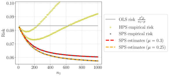
Figure 4: Our estimates for SPS match well with its empirical excess risk. In addition, the empirical risk of SPS is lower than HPS, especially in the negative transfer regime.

Simulations.

We perform a simulation to validate the limits in equations (4.16) and (4.17) in finite dimensions. In Figure 4, we use the same data-generating process as Figure 1. We find that SPS outperforms HPS, especially when the transfer effect is negative. This justifies the benefit of SPS over HPS in the presence of model shifts. Additionally, our estimates match well with the empirical risks in finite dimensions; here, $p$ is set as $100$.

Remark 4.7.

For a complete theory, it is desirable to derive the asymptotic bias and variance limits for the SPS estimator under 2.1 with arbitrary covariate shifts. This is a much more challenging problem and requires developing new tools beyond the current random matrix theory literature, which is left for future work.

4.3 Minimax lower bounds

Lastly, we complement our estimators with a minimax lower bound. Suppose we are trying to estimate an unknown parameter denoted as $\beta^{(2)}$. We are given $n_{2}$ samples drawn from a linear parametric model, following $\beta^{(2)}$, with isotropic Gaussian covariates $X^{(2)}$, contaminated by Gaussian noise with variance $\sigma^{2}$. Then, we are given $n_{1}$ samples from another linear parametric model, following $\beta^{(1)}$, again with isotropic Gaussian covariates $X^{(1)}$, contaminated by Gaussian noise with variance $\sigma^{2}$. The parameter vectors belong to the set $\Theta(\mu)=\{\beta^{(1)}\in{}^{p},\beta^{(2)}\in{}^{p}:\|{\beta^{(1)}-\beta^{(2)}}\|\leqslant\mu,\|{\beta^{(1)}}\|\leqslant 1,\|{\beta^{(2)}}\|\leqslant 1\}$. Note that our proof can be readily extended to cases with anisotropic Gaussian covariates as in (2.1), and the length constraints on ${\beta^{(1)}}$ and ${\beta^{(2)}}$ can be replaced with any other constant.

Let $\hat{\beta}$ be any estimation procedure that, given the above $n_{1}+n_{2}$ samples, produces an estimate of the unknown vector $\beta^{(2)}$. We prove the following minimax rate on the estimation error of $\hat{\theta}$.

Theorem 4.8.

In the setting described above, let $\hat{\beta}$ be some estimation procedure. Assume that $n_{1}\geqslant(1+\tau)p$ and $n_{2}\geqslant(1+\tau)p$ for a constant $\tau>0$. For any $(\beta^{(1)},\beta^{(2)})$ within the set $\Theta(\mu)$, with high probability over the randomness of $(X^{(1)},X^{(2)})$, we have that

$$\inf_{\hat{\beta}}\sup_{\Theta(\mu)}\mathop{\mathbb{E}}\left[\frac{1}{n_{2}}\left\|\widetilde{X}^{(2)}\left(\hat{\beta}-\beta^{(2)}\right)\right\|^{2}\right]\geqslant c{\Big{(}{\min\Big{(}\mu^{2},\frac{\sigma^{2}p}{n_{2}}\Big{)}+\frac{\sigma^{2}p}{n_{1}+n_{2}}}\Big{)}},$$ (4.18)

where the expectation is over the randomness of $(X^{(1)},X^{(2)},Y^{(1)},Y^{(2)})$ and an independently drawn $\widetilde{X}^{(2)}$ that follows the same distribution as $X^{(2)}$, and $c$ is a fixed constant that does not grow with $p$.

The lower bound in equation (4.18) involves two parts. For the second part, $\frac{\sigma^{2}p}{n_{1}+n_{2}}$ is the rate in the case without model drift, i.e., $\beta^{(1)}=\beta^{(2)}$. For the first part, if $\mu$ is large, the source samples are not helpful, so the rate $\frac{\sigma^{2}p}{n_{2}}$ is the OLS rate using only the target task samples. If $\mu$ is small and $n_{1}$ is large, then the rate $\mu^{2}$ appears if we use the OLS estimator for the source task. The detailed proof can be found in Section D.4.

It is easy to check that under assumptions (2.3) and (2.5), our estimates of the excess risks in Theorem 4.1 and Theorem 4.6 are of order $\mu^{2}+\frac{\sigma^{2}p}{n_{1}+n_{2}}$, which matches the lower bound in (4.18) when $\mu^{2}=\operatorname{O}(\frac{\sigma^{2}p}{n_{2}})$. If $\mu^{2}$ is much larger than $\frac{\sigma^{2}p}{n_{2}}$, the rates in Theorem 4.1 and Theorem 4.6 may not be optimal. But, the adjusted estimator in Section 4.1.2 always achieves the optimal rate. In fact, in the setting of Claim 4.4, the excess risk of the adjusted estimator is always less than $\ell(0)=\frac{\sigma^{2}p}{n_{2}-p}$, which is the desired rate when $\mu^{2}$ is large.

5 Extensions

We present two extensions to reinforce our findings from previous sections. These are by no means comprehensive, but we hope that they help justify that our theoretical insights carry over to more general settings beyond what we have considered.

5.1 Covariate and model shifts

We first consider a setting with both covariate and model shifts. Define a function that depends on the source task’s covariance:

$$g_{0}(x)=\frac{1}{n_{1}}\operatorname{Tr}\left[{\Sigma^{(1)}}\big{(}{\operatorname{Id}_{p\times p}+x\cdot\Sigma^{(1)}}\big{)}^{-1}\right]-\frac{1}{x}.$$ (5.1)

Let $g_{0}^{\prime}(x)$ be the derivative of $g_{0}(x)$. It can be shown that there is a unique positive solution to the equation

$$(1+x)g_{0}(x)=-n_{1}^{-1}(n_{1}+n_{2}-p).$$ (5.2)

Let $y_{0}$ denote this solution. The following theorem gives the exact asymptotic variance and bias limits when the target task’s population covariance is isotropic.

Theorem 5.1 (Exact estimates under covariate and model shifts).

Under Assumption 2.1, suppose that $\Sigma^{(2)}=\operatorname{Id}_{p\times p}$ and $Z^{(1)}$ and $Z^{(2)}$ are both Gaussian random matrices. Suppose further that the random-effects model applies. Let

$$f_{1}=\frac{n_{1}}{p}y_{0}+\frac{n_{1}-p}{p\cdot g_{0}(y_{0})},\ f_{2}=\frac{n_{1}}{p\cdot g_{0}^{\prime}(y_{0})}-\frac{n_{1}-p}{p\cdot(g_{0}(y_{0}))^{2}},\text{ and }f_{3}=-g_{0}(y_{0}).$$ (5.3)

Then, for any small constant ${\mathit{c}}>0$, with high probability over the randomness of training samples and model vectors, the following estimates hold:

$$L_{\text{var}}=\left(1+\operatorname{O}(p^{-1/2+c})\right)\cdot\sigma^{2}{p}n_{1}^{-1}f_{1},$$ (5.4)

$$L_{\text{bias}}=\left(1+\operatorname{O}(p^{-1/2+c})\right)\cdot 2\mu^{2}\frac{1-2f_{1}f_{3}+f_{2}f_{3}^{2}}{1-n_{2}^{-1}{p}f_{2}f_{3}^{2}}.$$ (5.5)

When the population covariance of the source task is also isotropic ($\Sigma^{(1)}=\operatorname{Id}_{p\times p}$), we can verify that the above result is consistent with the variance and bias limits in Theorem 4.1. The proof of Theorem 5.1 uses similar techniques as those in the proof of Theorem 4.1. It can be found in Section E.1.

The anisotropic case.

Theorem 5.1 states exact estimates when the target task’s population covariance is isotropic. In the general anisotropic case, it is possible to estimate the bias formula (2.9) by approximating the source task’s sample covariance matrix with its expectation. It turns out that this renders the analysis of the bias formula similar to that of the variance formula in Theorem 3.1. However, this approximation results in an error term that decreases to zero (relative to the estimated term) as $n_{1}/p$ increases to infinity; see the right-hand side of equation (C.4). Thus, the accuracy of the estimate increases as $n_{1}/p$ increases. This approximation is actually motivated by transfer learning scenarios with a large source task relative to the target task. The theorem statement together with a complete proof is described in length within Appendix C.2 (see Theorem C.1).

Numerical comparisons.

We complement our theoretical analysis of HPS with empirical evaluations. Figure 5 illustrates the result for a setting where half of the eigenvalues of $\Sigma^{(1)}$ are equal to $\lambda>1$ and the other half are equal to $1/\lambda$. Our theoretical estimates consistently match the empirical risks. Figure 5(a) shows a similar dichotomy as in Figure 2(b). We fix model shift $\mu=0.1$ while varying covariate shift $\lambda$ for each curve. Figure 5(b) illustrates different transfer effects as in Figure 1. We fix the level of covariate shift $\lambda=4$ while varying $\mu$ for each curve. Both simulations use $p=100,$ $n_{2}=300$, and $\sigma=1/2$.

In Figures 5(c) and 5(d), we generate covariate shifted features and different linear models for the two tasks. We take the average of 100 random seeds because of high variances due to small sample sizes. We find that HPS achieves superior performance under various settings of covariate and model shifts.

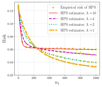
((a)) Varying covariate shift with fixed model shift

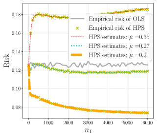
((b)) Varying model shift with fixed covariate shift

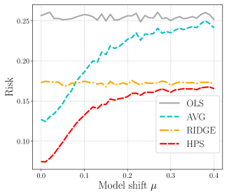
((c)) Varying model shift without covariate shift

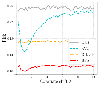
((d)) Varying covariate shift with fixed model shift

Figure 5: In Figures 5(a) and 5(b), we show that our findings from previous sections still hold with both covariate and model shifts. In Figures 5(c) and 5(d), we compare the empirical risks of HPS and several other estimators, showing that HPS achieves the lowest excess risk compared to OLS, AVG, and RIDGE. This simulation uses $p=50,n_{1}=n_{2}=100,$ and $\sigma=1/2$ in every figure. Figure 5(d) uses $\mu=0.05$ for simulating model shift.

5.2 Multiple source tasks

Next, we extend our findings to multiple source tasks. Suppose there are $t$ tasks whose feature covariates are all equal to $X\in{}^{n\times p}$. The label vector of the $i$-th task follows a linear model with an unknown $p$ dimensional vector $\beta^{(i)}$, for $i=1,2,\dots,t$:

$$Y^{(i)}=X\beta^{(i)}+\varepsilon^{(i)}.$$ (5.6)

Similar to the two-task case, one of the tasks is viewed as a primary target task of interest while the rest of them are used as source tasks that help with learning. Assume that $X=Z\Sigma^{1/2}\in{}^{n\times p}$ is a random matrix satisfying the same assumption as $X^{(2)}$ in Assumption 2.1, and $\varepsilon^{(i)}\in{}^{n}$, $i=1,2,\dots,t$, are independent random vectors, each of which is independent of $X$ and satisfies the same assumption as $\varepsilon^{(2)}$ in Assumption 2.1. Furthermore, each $\beta^{(i)}\in{}^{p}$ is a (random or deterministic) vector independent of any other $\beta^{(j)}$ for $j\neq i$, the matrix $X$, and $\varepsilon^{(j)}$ for all $j=1,\dots,t$. The sample size $n$ satisfies $1+\tau\leqslant n/p\leqslant p^{\tau^{-1}}$.

We combine all data sources with an HPS estimator as follows:

$$f(A,B)=\sum_{j=1}^{t}\left\|XBA_{j}-Y^{(j)}\right\|^{2},$$ (5.7)

where $A=[A_{1},A_{2},\dots,A_{t}]\in{}^{r\times t}$ denotes the output layer and $B\in{}^{p\times r}$ denotes the shared feature layer. The width of $B$ is denoted by $r$. We focus on the case of $r<t$. Otherwise, if $r\geqslant t$, the problem reduces to single-task learning (Wu et al., 2020, Proposition 1).

Let $(\hat{A},\hat{B})$ denote the global minimizer of $f(A,B)$. The HPS estimator is defined for task $i$ as $\hat{\beta}_{i}^{\textup{HPS}}=\hat{B}\hat{A}_{i}$, where $\hat{A}_{i}$ denotes the $i$-th column of $\hat{A}$. The excess risk of $\hat{\beta}_{i}^{\textup{HPS}}$ is equal to:

$$L_{i}(\hat{\beta}_{i}^{\textup{HPS}})=\left\|\Sigma^{1/2}\left(\hat{\beta}^{\textup{HPS}}_{i}-\beta^{(i)}\right)\right\|^{2}.$$ (5.8)

5.2.1 Results

We show that in the above multi-task setting, hard parameter sharing finds the best rank-$r$ approximation in some sense. To describe the result, we introduce several notations. Let $B^{\star}:=[{\beta}^{(1)},{\beta}^{(2)},\dots,{\beta}^{(t)}]\in{}^{p\times t}$ be the matrix of concatenated model vectors. Let $A^{\star}{A^{\star}}^{\top}$ be the best approximation of ${B^{\star}}^{\top}\Sigma B^{\star}$ in the set of rank-$r$ subspaces:

$$A^{\star}:=\mathop{\textup{argmax}}_{U\in{}^{t\times r}:\ U^{\top}U=\operatorname{Id}_{r\times r}}\langle UU^{\top},{B^{\star}}^{\top}\Sigma B^{\star}\rangle,$$ (5.9)

where $\langle\cdot,\cdot\rangle$ denotes the Frobenius inner product between two matrices. Let $a_{i}^{\star}\in{}^{r}$ be the $i$-th column vector of $A^{\star}{A^{\star}}^{\top}$. For any matrix $X$, let $\|X\|_{2}$ be its spectral norm and $\|X\|_{F}$ be its Frobenius norm. A precise estimate of the excess risk of HPS is stated below.

Theorem 5.2 (HPS for multiple tasks).

Suppose the setting described above holds. Let $r<t$ be a positive integer. Suppose the $r$-th largest eigenvalue $\lambda_{r}$ of ${B^{\star}}^{\top}\Sigma B^{\star}$ is strictly larger than its $(r+1)$-th largest eigenvalue $\lambda_{r+1}$. Then, for $i=1,\dots,t$ and any small constant $c>0$, the following estimate holds with high probability over the randomness of the training samples:

$$\left|{L_{i}(\hat{\beta}_{i}^{\textup{HPS}})-L_{i}(B^{\star}a_{i}^{\star})-\frac{\sigma^{2}p\left\|a_{i}^{\star}\right\|^{2}}{n-p}}\right|\leqslant\Big{(}{\|{B^{\star}}^{\top}\Sigma B^{\star}\|_{2}+\sigma^{2}}\Big{)}\sqrt{\frac{\|{B^{\star}}^{\top}\Sigma B^{\star}\|_{2}\cdot n^{\frac{2}{\varphi}-\frac{1}{2}+c}+\sigma^{2}n^{-\frac{1}{2}+c}}{\lambda_{r}-\lambda_{r+1}}}.$$ (5.10)

In equation (5.10), $L_{i}(B^{\star}a_{i}^{\star})$ is the asymptotic bias limit, while $\frac{\sigma^{2}p}{n-p}\left\|a_{i}^{\star}\right\|^{2}$ is the asymptotic variance limit. The proof of Theorem 5.2 relies on a characterization of the global minimizer of problem (5.7) through a connection to PCA. The detailed proof can be found in Appendix E.2.

Remark 5.3.

The data model studied in this setting (cf. equation (5.6)) has been studied in a sparse setting where all model vectors ($\beta^{(1)},\dots,\beta^{(t)}$) share the same support of nonzero coordinates (Lounici et al., 2011). Notice that our result does not require this condition. Independent of this paper, Duan and Wang (2022) examine a multitask learning setting and provide an adaptive estimation procedure to select beneficial source tasks given multiple tasks.

Remark 5.4.

The setting for Theorem 5.2 only involves model shifts. It is an interesting question to study covariate shifts in the multitask setting. We leave it to future works.

5.2.2 Examples

We illustrate the above result with the random-effects model again. The model vector of every task is equal to a shared vector $\beta_{0}$ plus a task-specific component $\gamma_{i}$, for $i=1,2,\cdots,t$:

$$\beta^{(i)}=\beta_{0}+\gamma_{i}.$$ (5.11)

The entries of $\gamma_{i}$ are drawn independently from a Gaussian distribution with mean zero and variance $p^{-1}\mu^{2}$. We study two natural questions:

1. What is the optimal width $r$ of the shared feature layer $B$?

2. When does HPS transfer positively to a particular task, depending on the sample size $n$ and the model shift parameter $\mu$?

For the first question, since the setting is symmetric in the $t$ tasks, we analyze the averaged limiting risk

$$g_{r}(n,\mu):=\frac{1}{t}\left\|\Sigma^{1/2}B^{\star}(A^{\star}{A^{\star}}^{\top}-\operatorname{Id}_{t\times t})\right\|_{F}^{2}+\frac{\sigma^{2}p}{n-p}\frac{r}{t},$$

which accurately approximates $t^{-1}\sum_{i=1}^{t}L_{i}(\hat{\beta}_{i}^{\textup{HPS}})$ by Theorem 5.2. To see this, we notice that the average of the bias and variance limits in equation (5.10) is

$$\frac{1}{t}\sum_{i=1}^{t}\left(L_{i}(B^{\star}a_{i}^{\star})+\frac{\sigma^{2}p}{n-p}\left\|a_{i}^{\star}\right\|^{2}\right)=\frac{1}{t}\left\|\Sigma^{1/2}B^{\star}(A^{\star}{A^{\star}}^{\top}-\operatorname{Id}_{t\times t})\right\|_{F}^{2}+\frac{\sigma^{2}p}{n-p}\frac{r}{t}.$$

Above, we have used the matrix notation $A^{\star}$ to rewrite the bias component. Moreover, we apply the identity $\sum_{i=1}^{t}\|a_{i}^{\star}\|^{2}=\operatorname{Tr}[(A^{\star}{A^{\star}}^{\top})^{2}]=r$ to the variance component, since ${A^{\star}}^{\top}A^{\star}=\operatorname{Id}_{r\times r}$ following definition (5.9). Then, optimal width can be identified by sweeping through $g_{r}(n,\mu)$ for different values of $r$.

For the second question, recall that by equation (3.3), the excess risk of the OLS estimator is given by $\sigma^{2}\frac{p}{n-p}$. Thus, by comparing $g_{r}(n,\mu)$ to $\sigma^{2}\frac{p}{n-p}$, the exact threshold between positive and negative transfer can be identified. This is stated in the following result, proved in Section E.3.

Proposition 5.5 (Effect of model shift with multiple tasks).

Suppose the multitask setting holds. Assume further the random-effects model in equation (5.11) holds. Then, for any small constant $c>0$, the following claims hold with high probability over the randomness of the training samples and the model vectors:

1. When $\mu^{2}>\left(1+p^{-1/2+c}\right)\frac{\sigma^{2}p^{2}}{(n-p)\operatorname{Tr}[\Sigma]}$, then $g_{r}(n,\mu)\geqslant\frac{\sigma^{2}p}{n-p}$ for any $1\leqslant r<t$.

2. When $\mu^{2}<\left(1-p^{-1/2+c}\right)\frac{\sigma^{2}p^{2}}{(n-p)\operatorname{Tr}[\Sigma]}$, then $g_{r}(n,\mu)$ is minimized when $r=1$; further, $g_{1}(n,\mu)\leqslant\frac{\sigma^{2}p}{n-p}$.

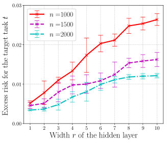
((a)) Varying the width of the shared layer

((b)) Varying model vector’s Euclidean distance

Figure 6: Illustration of transfer effects in the random-effects model with multiple source tasks. Figure 6(a) shows that for hidden layer width $r$ from 1 to 10, the lowest excess risk of task $t$ is achieved at 1 (averaged over three random seeds). Figure 6(b) fixes width as one and varies model shift and sample size. Similar to Figure 1, HPS may provide a positive or negative transfer to task $t$ depending on $\mu$ and $n$.

Figure 6 illustrates the above result with ten tasks of dimension $p=100$ and noise variance $\sigma=1/2$. We plot the theoretical estimate using $g_{r}(n,\mu)$ and the empirical risk using the bias plus variance of $\hat{\beta}_{t}^{\textup{HPS}}$ (cf. equation (E.22) in Section E.2). Figure 6(a) shows that the empirical risk for predicting task $t$ is indeed minimized when $r=1$. Figure 6(b) shows different transfer effects by varying $n$ and $\mu$ in the multitask setting. The results under different values of $\mu$ also match the conditions in Proposition 5.5.

6 Conclusion

This paper provides several high-dimensional asymptotic results for the analysis of transfer learning in linear regression. The main technical ingredients involve estimating the high-dimensional asymptotics for functions of two independent sample covariance matrices under various combinations of covariate and model shifts. Numerical simulations are provided to justify the validity of these asymptotic limits in finite dimensions. We hope our work will inspire future studies on the interplay between random matrix theory and transfer learning.

Appendix A Basic tools

In this supplement, we will use the following notations. The fundamental large parameter in our proof is $p$. All quantities that are not explicitly constant may depend on $p$, and we usually omit $p$ from our notations. Given any matrix $X$, let $\lambda_{\min}(X)$ denote its smallest singular value and $\|X\|$ denote its largest singular value (or equivalently, the operator norm); let $\lambda_{1}(X)\geqslant\lambda_{2}(X)\geqslant\cdots$ denote the singular values of $X$ in descending order; let $X^{+}$ denote the Moore-Penrose pseudoinverse of $X$. As a special case, the operator norm of a vector $v$ is also its Euclidean norm, i.e., $\|v\|=\|v\|_{2}$. We say an event $\Xi$ holds with high probability if $\mathbb{P}(\Xi)\to 1$ as $p\to\infty$. We will use the big-O notation $g(p)=\operatorname{O}(f(p))$ if there exists a constant $C>0$ such that $|g(p)|\leqslant Cf(p)$ for large enough $p$. Moreover, for any $g(p)\geqslant 0$ and $f(p)\geqslant 0$, we will use the notations $g(p)\lesssim f(p)$ if $g(p)=\operatorname{O}(f(p))$, and $g(p)\sim f(p)$ if $g(p)\lesssim f(p)$ and $f(p)\lesssim g(p)$. We will often write an identity matrix as $1$ without causing any confusion.

In this section, we collect some useful tools that will be used in the proof. First, it is convenient to introduce the following notation.

Definition A.1 (Overwhelming probability).

We say an event $\Xi$ holds with overwhelming probability (w.o.p.) if for any constant $D>0$, $\mathbb{P}(\Xi)\geqslant 1-p^{-D}$ for large enough $p$. Moreover, we say $\Xi$ holds with overwhelming probability in an event $\Omega$ if for any constant $D>0$, $\mathbb{P}(\Omega\setminus\Xi)\leqslant p^{-D}$ for large enough $p$.

The following notion of stochastic domination, which was first introduced in Erdős et al. [2013a], is commonly used in the study of random matrices.

Definition A.2 (Stochastic domination).

Let $\xi\equiv\xi^{(p)}$ and $\zeta\equiv\zeta^{(p)}$ be two $p$-dependent random variables. We say that $\xi$ is stochastically dominated by $\zeta$, denoted by $\xi\prec\zeta$ or $\xi=\operatorname{O}_{\prec}(\zeta)$, if for any small constant ${\mathit{c}}>0$ and large constant $D>0$, there exists a $p_{0}({\mathit{c}},D)\in\mathbb{N}$ such that for all $p>p_{0}({\mathit{c}},D)$,

$$\operatorname{\mathbb{P}}\left(|\xi|>p^{\mathit{c}}|\zeta|\right)\leqslant p^{-D}.$$

In other words, $\xi\prec\zeta$ if $|\xi|\leqslant p^{\mathit{c}}|\zeta|$ with overwhelming probability for any small constant ${\mathit{c}}>0$. If $\xi(u)$ and $\zeta(u)$ are functions of $u$ supported in a set $\mathcal{U}$, then we say $\xi(u)$ is stochastically dominated by $\zeta(u)$ uniformly in $\mathcal{U}$ if

$$\operatorname{\mathbb{P}}\left(\cup_{u\in\mathcal{U}}\{|\xi(u)|>p^{\mathit{c}}|\zeta(u)|\}\right)\leqslant p^{-D}$$

for large enough $p$. Given any event $\Omega$, we say $\xi\prec\zeta$ on $\Omega$ if $\mathbf{1}_{\Omega}\xi\prec\zeta$.

Remark A.3.

We make two simple remarks. First, since we allow for an $p^{\mathit{c}}$ factor in stochastic domination, we can ignore $\log$ factors without loss of generality since $(\log p)^{C}\prec 1$ for any constant $C>0$. Second, given a random variable $\xi$ with unit variance and finite moments up to any order as in (2.4), we have that $|\xi|\prec 1$. This is because, by Markov’s inequality, there is

$$\mathbb{P}(|\xi|\geqslant p^{{\mathit{c}}})\leqslant p^{-k{\mathit{c}}}{\mathbb{E}|\xi|^{k}}\leqslant p^{-D},$$

as long as $k$ is taken to be larger than $D/{\mathit{c}}$.

The following lemma collects several basic properties of stochastic domination that will be used tacitly in the proof. Roughly speaking, it says that the stochastic domination “$\prec$" can be treated as the conventional less-than sign “$<$" in some sense.

Lemma A.4 (Lemma 3.2 in Bloemendal et al. [2014]).

Let $\xi$ and $\zeta$ be two families of nonnegative random variables depending on some parameters $u\in\mathcal{U}$ and $v\in\mathcal{V}$. Let $C>0$ be an arbitrary constant.

• Sum. Suppose that $\xi(u,v)\prec\zeta(u,v)$ uniformly in $u\in\mathcal{U}$ and $v\in\mathcal{V}$. If $|\mathcal{V}|\leqslant p^{C}$, then $\sum_{v\in\mathcal{V}}\xi(u,v)\prec\sum_{v\in\mathcal{V}}\zeta(u,v)$ uniformly in $u$.

• Product. If $\xi_{1}(u)\prec\zeta_{1}(u)$ and $\xi_{2}(u)\prec\zeta_{2}(u)$ uniformly in $u\in\mathcal{U}$, then $\xi_{1}(u)\xi_{2}(u)\prec\zeta_{1}(u)\zeta_{2}(u)$ uniformly in $u\in\mathcal{U}$.

• Expectation. Suppose that $\Psi(u)\geqslant p^{-C}$ is a family of deterministic parameters, and $\xi(u)$ satisfies $\mathbb{E}\xi(u)^{2}\leqslant p^{C}$. If $\xi(u)\prec\Psi(u)$ uniformly in $u$, then we also have $\mathbb{E}\xi(u)\prec\Psi(u)$ uniformly in $u$.

Let $Q>0$ be a ($p$-dependent) deterministic parameter. We say a random matrix $Z\in{}^{n\times p}$ satisfies the bounded support condition with $Q$ (or $Z$ has bounded support $Q$) if

$$\max_{1\leqslant i\leqslant n,1\leqslant j\leqslant p}|Z_{ij}|\prec Q.$$ (A.1)

As shown in Remark A.3, if the entries of $Z$ have finite moments up to any order, then $Z$ has bounded support $Q=1$. More generally, if every entry of $Z$ has a finite $\varphi$-th moment as in (2.2) and $n\geqslant p$, then using Markov’s inequality and a simple union bound we get that

$$\mathbb{P}\left(\max_{1\leqslant i\leqslant n,1\leqslant j\leqslant p}|Z_{ij}|\geqslant(\log n)n^{\frac{2}{\varphi}}\right) \leqslant\sum_{i=1}^{n}\sum_{j=1}^{p}\mathbb{P}\left(|Z_{ij}|\geqslant(\log n)n^{\frac{2}{\varphi}}\right)$$

$$\lesssim\sum_{i=1}^{n}\sum_{j=1}^{p}\left[(\log n)n^{\frac{2}{\varphi}}\right]^{-\varphi}\leqslant(\log n)^{-\varphi}.$$ (A.2)

In other words, $Z$ has bounded support $Q=n^{{2}/{\varphi}}$ with high probability.

The following lemma gives sharp concentration bounds for linear and quadratic forms of random variables with bounded support.

Lemma A.5 (Lemma 3.8 of Erdős et al. [2013c] and Theorem B.1 of Erdős et al. [2013b]).

Let $(x_{i})$, $(y_{j})$ be families of centered and independent random variables, and $(A_{i})$, $(B_{ij})$ be families of deterministic complex numbers. Suppose the entries $x_{i}$ and $y_{j}$ have variance at most $1$, and satisfy the bounded support condition (A.1) for a deterministic parameter $Q\geqslant 1$. Then, we have the following estimates:

$$\Big{|}\sum_{i=1}^{n}A_{i}x_{i}\Big{|}\prec Q\max_{i=1}^{n}|A_{i}|+\Big{(}\sum_{i=1}^{n}|A_{i}|^{2}\Big{)}^{1/2},$$ (A.3)

$$\Big{|}\sum_{i,j=1}^{n}x_{i}B_{ij}y_{j}\Big{|}\prec Q^{2}B_{d}+Qn^{1/2}B_{o}+\Big{(}\sum_{1\leqslant i\neq j\leqslant n}|B_{ij}|^{2}\Big{)}^{{1}/{2}},$$ (A.4)

$$\Big{|}\sum_{i=1}^{n}(|x_{i}|^{2}-\mathbb{E}|x_{i}|^{2})B_{ii}\Big{|}\prec Qn^{1/2}B_{d},$$ (A.5)

$$\Big{|}\sum_{1\leqslant i\neq j\leqslant n}x_{i}B_{ij}x_{j}\Big{|}\prec Qn^{1/2}B_{o}+\Big{(}\sum_{1\leqslant i\neq j\leqslant n}|B_{ij}|^{2}\Big{)}^{{1}/{2}},$$ (A.6)

where we denote $B_{d}:=\max_{i}|B_{ii}|$ and $B_{o}:=\max_{i\neq j}|B_{ij}|.$ Moreover, if $x_{i}$ and $y_{j}$ have finite moments up to any order, then we have the following stronger estimates:

$$\Big{|}\sum_{i=1}^{n}A_{i}x_{i}\Big{|}\prec\Big{(}\sum_{i=1}^{n}|A_{i}|^{2}\Big{)}^{1/2},$$ (A.7)

$$\Big{|}\sum_{i,j=1}^{n}x_{i}B_{ij}y_{j}\Big{|}\prec\Big{(}\sum_{i,j=1}^{n}|B_{ij}|^{2}\Big{)}^{{1}/{2}},$$ (A.8)

$$\Big{|}\sum_{i=1}^{n}(|x_{i}|^{2}-\mathbb{E}|x_{i}|^{2})B_{ii}\Big{|}\prec\Big{(}\sum_{i=1}^{n}|B_{ii}|^{2}\Big{)}^{1/2},$$ (A.9)

$$\Big{|}\sum_{1\leqslant i\neq j\leqslant n}x_{i}B_{ij}x_{j}\Big{|}\prec\Big{(}\sum_{1\leqslant i\neq j\leqslant n}|B_{ij}|^{2}\Big{)}^{{1}/{2}}.$$ (A.10)

It is well-known that the empirical spectral distributions of ${Z^{(1)}}^{\top}Z^{(1)}$ and ${Z^{(2)}}^{\top}Z^{(2)}$ satisfy the Marchenko-Pastur (MP) law [Marčenko and Pastur, 1967]. Moreover, their eigenvalues are all inside the support of the MP law with high probability [Bai and Silverstein, 1998]. In the proof, we will need a slightly stronger result that holds with overwhelming probability as given by the following lemma.

Lemma A.6.

Suppose $Z\in\mathbb{R}^{n\times p}$ is an $n\times p$ random matrix satisfying the same assumptions as $Z^{(2)}$ in Assumption 2.1. Suppose $1+\tau\leqslant{n}/{p}\leqslant p^{\tau^{-1}}$, and $Z$ satisfies the bounded support condition (A.1) for a deterministic parameter $Q$ such that $1\leqslant Q\leqslant n^{1/2-c_{Q}}$ for a constant $c_{Q}>0$. Then, we have that

$$(\sqrt{n}-\sqrt{p})^{2}-\operatorname{O}_{\prec}(\sqrt{n}\cdot Q)\leqslant\lambda_{p}(Z^{\top}Z)\leqslant\lambda_{1}(Z^{\top}Z)\leqslant(\sqrt{n}-\sqrt{p})^{2}+\operatorname{O}_{\prec}(\sqrt{n}\cdot Q).$$ (A.11)

Proof.

When $Q$ is of order 1, this lemma follows from Theorem 2.10 of Bloemendal et al. [2014]. The result for the general case with $1\leqslant Q\leqslant n^{1/2-c_{Q}}$ follows from Lemma 3.11 of Ding and Yang [2018]. ∎

Using a standard cut-off argument, we can extend Lemma A.5 and Lemma A.6 to random matrices whose entries satisfy only certain moment assumptions but not necessarily the bounded support condition.

Corollary A.7.

Suppose $Z\in\mathbb{R}^{n\times p}$ is an $n\times p$ random matrix satisfying the same assumptions as $Z^{(2)}$ in Assumption 2.1. Suppose $1+\tau\leqslant{n}/{p}\leqslant p^{\tau^{-1}}$. Then, (A.11) holds on a high probability event with $Q=n^{2/\varphi}$, where $\varphi$ is the constant in (2.2).

Proof.

We introduce a truncated matrix $\widetilde{Z}$ with entries

$$\widetilde{Z}_{ij}:=\mathbf{1}\left(|Z_{ij}|\leqslant Q\log n\right)\cdot Z_{ij}.$$ (A.12)

From equation (A.2), we get that

$$\mathbb{P}(\widetilde{Z}=Z)=1-\mathbb{P}\left(\max_{i,j}|Z_{ij}|>Q\log n\right)=1-\operatorname{O}((\log n)^{-\varphi}).$$ (A.13)

By definition, we have

$$\begin{split}\mathbb{E}\widetilde{Z}_{ij}&=-\mathbb{E}\left[\mathbf{1}\left(|Z_{ij}|>Q\log n\right)Z_{ij}\right],\\ \mathbb{E}|\widetilde{Z}_{ij}|^{2}&=1-\mathbb{E}\left[\mathbf{1}\left(|Z_{ij}|>Q\log n\right)|Z_{ij}|^{2}\right].\end{split}$$ (A.14)

Using the tail probability expectation formula, we can check that

$$\mathbb{E}\left|\mathbf{1}\left(|Z_{ij}|>Q\log n\right)Z_{ij}\right|=\int_{0}^{\infty}\mathbb{P}\left(\left|\mathbf{1}\left(|Z_{ij}|>Q\log n\right)Z_{ij}\right|>s\right)\mathrm{d}s$$

$$=\int_{0}^{Q\log n}\mathbb{P}\left(|Z_{ij}|>Q\log n\right)\mathrm{d}s+\int_{Q\log n}^{\infty}\mathbb{P}\left(|Z_{ij}|>s\right)\mathrm{d}s$$

$$\lesssim\int_{0}^{Q\log n}\left(Q\log n\right)^{-\varphi}\mathrm{d}s+\int_{Q\log n}^{\infty}s^{-\varphi}\mathrm{d}s\leqslant n^{-2(\varphi-1)/\varphi},$$

where in the third step we use the finite $\varphi$-th moment condition (2.2) for $Z_{ij}$ and Markov’s inequality. Similarly, we can obtain that

$$\mathbb{E}\left|\mathbf{1}\left(|Z_{ij}|>Q\log n\right)Z_{ij}\right|^{2}=2\int_{0}^{\infty}s\mathbb{P}\left(\left|\mathbf{1}\left(|Z_{ij}|>Q\log n\right)Z_{ij}\right|>s\right)\mathrm{d}s$$

$$=2\int_{0}^{Q\log n}s\mathbb{P}\left(|Z_{ij}|>Q\log n\right)\mathrm{d}s+2\int_{Q\log n}^{\infty}s\mathbb{P}\left(|Z_{ij}|>s\right)\mathrm{d}s$$

$$\lesssim\int_{0}^{Q\log n}s\left(Q\log n\right)^{-\varphi}\mathrm{d}s+\int_{Q\log n}^{\infty}s^{-\varphi+1}\mathrm{d}s\leqslant n^{-2(\varphi-2)/\varphi}.$$

Plugging the above two estimates into (A.14) and using $\varphi>4$, we get that

$$|\mathbb{E}\widetilde{Z}_{ij}|=\operatorname{O}(n^{-3/2}),\quad\mathbb{E}|\widetilde{Z}_{ij}|^{2}=1+\operatorname{O}(n^{-1}).$$ (A.15)

From the first estimate in equation (A.15), we also get a bound on the operator norm:

$$\|\mathbb{E}\widetilde{Z}\|=\operatorname{O}(n^{-1/2}).$$ (A.16)

Then, we centralize and rescale $\widetilde{Z}$ as

$$\widehat{Z}:=(\widetilde{Z}-\mathbb{E}\widetilde{Z})/\sqrt{\mathbb{E}|\widetilde{Z}_{11}|^{2}}.$$ (A.17)

Now, $\widehat{Z}$ is a matrix satisfying the assumptions of Lemma A.6 with bounded support $Q$. Thus, we get that

$$(\sqrt{n}-\sqrt{p})^{2}-\operatorname{O}_{\prec}(\sqrt{n}\cdot Q)\leqslant\lambda_{p}(\widehat{Z}^{\top}\widehat{Z})\leqslant\lambda_{1}(\widehat{Z}^{\top}\widehat{Z})\leqslant(\sqrt{n}-\sqrt{p})^{2}+\operatorname{O}_{\prec}(\sqrt{n}\cdot Q).$$

Combining this estimate with (A.15) and (A.16), we can readily get that (A.11) holds for the eigenvalues of $\widetilde{Z}^{\top}\widetilde{Z}$, which concludes the proof by (A.13). ∎

Corollary A.8.

Suppose $Z\in\mathbb{R}^{n\times p}$ is an $n\times p$ random matrix satisfying the same assumptions as $Z^{(2)}$ in Assumption 2.1. Then, there exists a high probability event on which the following estimate holds for any deterministic vector $v\in\mathbb{R}^{p}$:

$$\left|\|Zv\|^{2}-n\|v\|^{2}\right|\prec n^{1/2}Q\|v\|^{2},\quad\text{for}\quad Q=n^{2/\varphi}.$$ (A.18)

Proof.

Similar to the proof of Corollary A.7, we truncate $Z$ as in (A.12) and define $\widehat{Z}$ by (A.17). By (A.15) and (A.16), we see that to conclude (A.18), it suffices to show that

$$\left|\|\widehat{Z}v\|^{2}-n\|v\|^{2}\right|\prec n^{1/2}Q\|v\|^{2}.$$ (A.19)

To prove equation (A.19), we first notice that $\widehat{Z}v\in\mathbb{R}^{n}$ is a random vector with i.i.d. entries of mean zero and variance $\|v\|^{2}$. Furthermore, with equation (A.3) we get that

$$|(\widehat{Z}v)_{i}|\prec Q\max_{j=1}^{p}|v_{j}|+\|v\|\leqslant 2Q\|v\|,\quad i=1,2,\cdots,n.$$

Hence, ${(\widehat{Z}v)}/{\|v\|}$ consists of i.i.d. random entries with zero mean, unit variance, and bounded support $Q$. Then, applying equation (A.5), we get that

$$\left|\|\widehat{Z}v\|^{2}-n\|v\|^{2}\right|=\|v\|^{2}\left|\sum_{i=1}^{n}\left(\frac{|(\widehat{Z}v)_{i}|^{2}}{\|v\|^{2}}-\mathbb{E}\frac{|(\widehat{Z}v)_{i}|^{2}}{\|v\|^{2}}\right)\right|\prec Qn^{1/2}\|v\|^{2}.$$

This concludes the proof. ∎

From Lemma A.5, we immediately obtain the following concentration estimates for the noise vectors.

Corollary A.9.

Suppose ${\varepsilon}^{(1)},\cdots,{\varepsilon}^{(t)}\in\mathbb{R}^{n}$ are independent random vectors satisfying Assumption 2.1 (ii). Then, we have that for any deterministic vector $v\in\mathbb{R}^{n}$,

$$|v^{\top}\varepsilon^{(i)}|\prec\sigma\|v\|,\quad i=1,\cdots,t,$$ (A.20)

and for any deterministic matrix $B\in{}^{n\times n}$,

$$\left|(\varepsilon^{(i)})^{\top}B\varepsilon^{(j)}-\delta_{ij}\cdot\sigma^{2}\operatorname{Tr}(B)\right|\prec\sigma^{2}\|B\|_{F},\quad i,j=1,\cdots,t.$$ (A.21)

Proof.

Note that $\varepsilon^{(i)}/\sigma$ is a random vector with i.i.d. entries of zero mean, unit variance, and bounded moments up to any order. Then, the bound (A.20) is an immediate consequence of equation (A.7). Using equation (A.8), we obtain that for $i\neq j$,

$$\left|(\varepsilon^{(i)})^{\top}B\varepsilon^{(j)}\right|=\Big{|}\sum_{k,l=1}^{n}\varepsilon^{(i)}_{k}\varepsilon^{(j)}_{l}B_{kl}\Big{|}\prec\sigma^{2}\Big{(}\sum_{k,l=1}^{n}|B_{kl}|^{2}\Big{)}^{1/2}=\sigma^{2}\|B\|_{F}.$$

Using the two estimates (A.9) and (A.10), we obtain that

$$\left|(\varepsilon^{(i)})^{\top}B\varepsilon^{(i)}-\sigma^{2}\operatorname{Tr}(B)\right| \leqslant\Big{|}\sum_{k}\left(|\varepsilon^{(i)}_{k}|^{2}-\mathbb{E}|\varepsilon^{(i)}_{k}|^{2}\right)B_{kk}\Big{|}+\Big{|}\sum_{k\neq l}\varepsilon^{(i)}_{k}\varepsilon^{(i)}_{l}B_{kl}\Big{|}$$

$$\prec\sigma^{2}\Big{(}\sum_{k}|B_{kk}|^{2}\Big{)}+\sigma^{2}\Big{(}\sum_{k\neq l}|B_{kl}|^{2}\Big{)}^{1/2}\lesssim\sigma^{2}\|B\|_{F}.$$

Hence, we have proved the bound (A.21). ∎

Appendix B Omitted proofs from Section 2

Proof of Lemma 2.2.

For the optimization objective $f(B)$ in equation (1.2), using the local optimality condition ${\partial f}/{\partial B}=0$, we can solve that

$$\hat{B}=\hat{\Sigma}^{-1}\left({X^{(1)}}^{\top}Y^{(1)}+{X^{(2)}}^{\top}Y^{(2)}\right),$$ (B.1)

where $\hat{\Sigma}$ is defined in (2.7). Then, the HPS estimator for task two is equal to

$$\hat{\beta}_{2}^{\textup{HPS}}=\hat{B}=\hat{\Sigma}^{-1}\left({X^{(1)}}^{\top}Y^{(1)}+{X^{(2)}}^{\top}Y^{(2)}\right).$$ (B.2)

Plugging (B.2) into the definition (2.6) of the excess risk, we get that

$$L(\hat{\beta}_{2}^{\textup{HPS}})= \left\|{\Sigma^{(2)}}^{1/2}\hat{\Sigma}^{-1}{X^{(1)}}^{\top}X^{(1)}(\beta^{(1)}-\beta^{(2)})+{\Sigma^{(2)}}^{1/2}\hat{\Sigma}^{-1}\left({X^{(1)}}^{\top}\varepsilon^{(1)}+{X^{(2)}}^{\top}\varepsilon^{(2)}\right)\right\|^{2}.$$ (B.3)

We expand the RHS as

$$L(\hat{\beta}_{2}^{\textup{HPS}})=L_{\text{bias}}+2h_{1}+2h_{2}+h_{3}+h_{4}+2h_{5},$$ (B.4)

where

$$h_{1}:={\varepsilon^{(1)}}^{\top}X^{(1)}\hat{\Sigma}^{-1}\Sigma^{(2)}\hat{\Sigma}^{-1}{X^{(1)}}^{\top}X^{(1)}(\beta^{(1)}-\beta^{(2)}),$$

$$h_{2}:={\varepsilon^{(2)}}^{\top}X^{(2)}\hat{\Sigma}^{-1}\Sigma^{(2)}\hat{\Sigma}^{-1}{X^{(1)}}^{\top}X^{(1)}(\beta^{(1)}-\beta^{(2)}),$$

$$h_{3}:={\varepsilon^{(1)}}^{\top}X^{(1)}\hat{\Sigma}^{-1}\Sigma^{(2)}\hat{\Sigma}^{-1}{X^{(1)}}^{\top}\varepsilon^{(1)},$$

$$h_{4}:={\varepsilon^{(2)}}^{\top}X^{(2)}\hat{\Sigma}^{-1}\Sigma^{(2)}\hat{\Sigma}^{-1}{X^{(2)}}^{\top}\varepsilon^{(2)},$$

$$h_{5}:={\varepsilon^{(1)}}^{\top}X^{(1)}\hat{\Sigma}^{-1}\Sigma^{(2)}\hat{\Sigma}^{-1}{X^{(2)}}^{\top}\varepsilon^{(2)}.$$

We estimate these terms one by one using Corollary A.9. In the proof, we will use the following estimates, which can be proved easily using the assumption (2.3) and Corollary A.7: on a high probability event $\Xi_{1}$,

$$\|X^{(1)}\|\lesssim\sqrt{n_{1}},\quad\|X^{(2)}\|\lesssim\sqrt{n_{2}},\quad\|\hat{\Sigma}^{-1}\|\lesssim(n_{1}+n_{2})^{-1},$$ (B.5)

and

$$L_{\text{bias}}\sim\frac{n_{1}^{2}}{(n_{1}+n_{2})^{2}}\left\|\beta^{(1)}-\beta^{(2)}\right\|^{2},\quad L_{\text{var}}\sim\frac{p\sigma^{2}}{n_{1}+n_{2}}.$$ (B.6)

Throughout the following proof, we assume that the event $\Xi_{1}$ holds.

Using (A.20), we can bound $h_{1}$ as

$$\left|h_{1}\right| \prec\sigma\left\|X^{(1)}\hat{\Sigma}^{-1}\Sigma^{(2)}\hat{\Sigma}^{-1}{X^{(1)}}^{\top}X^{(1)}(\beta^{(1)}-\beta^{(2)})\right\|$$

$$\lesssim\sigma\left\|\beta^{(1)}-\beta^{(2)}\right\|\cdot\left\|X^{(1)}\hat{\Sigma}^{-1}\Sigma^{(2)}\hat{\Sigma}^{-1}{X^{(1)}}^{\top}X^{(1)}\right\|$$

$$\lesssim\frac{\sigma\left\|\beta^{(1)}-\beta^{(2)}\right\|n_{1}^{3/2}}{(n_{1}+n_{2})^{2}}\leqslant\frac{p^{-1/4}n_{1}\left\|\beta^{(1)}-\beta^{(2)}\right\|}{n_{1}+n_{2}}\cdot\frac{p^{1/4}\sigma}{(n_{1}+n_{2})^{1/2}}$$

$$\leqslant\frac{p^{-1/2}n_{1}^{2}\left\|\beta^{(1)}-\beta^{(2)}\right\|^{2}}{(n_{1}+n_{2})^{2}}+\frac{p^{1/2}\sigma^{2}}{n_{1}+n_{2}}\lesssim p^{-1/2}\left(L_{\text{bias}}+L_{\text{var}}\right),$$

where we used (2.3) and (B.5) in the third step, the AM-GM inequality in the fifth step, and (B.6) in the last step. Similarly, we can show that

$$\left|h_{2}\right|\prec p^{-1/2}\left(L_{\text{bias}}+L_{\text{var}}\right).$$

Using (A.21), we can estimate $h_{3}$ as

$$\left|h_{3}-\sigma^{2}\operatorname{Tr}\left[X^{(1)}\hat{\Sigma}^{-1}\Sigma^{(2)}\hat{\Sigma}^{-1}{X^{(1)}}^{\top}\right]\right|$$

$$\prec\sigma^{2}\left\|X^{(1)}\hat{\Sigma}^{-1}\Sigma^{(2)}\hat{\Sigma}^{-1}{X^{(1)}}^{\top}\right\|_{F}\lesssim\frac{\sigma^{2}}{(n_{1}+n_{2})^{2}}\left\|X^{(1)}{X^{(1)}}^{\top}\right\|_{F}$$

$$\lesssim\frac{\sigma^{2}p^{1/2}n_{1}}{(n_{1}+n_{2})^{2}}\leqslant\frac{\sigma^{2}p^{1/2}}{n_{1}+n_{2}}\lesssim p^{-1/2}L_{\text{var}},$$

where we used (2.3) and (B.5) in the second step, and

$$\left\|X^{(1)}{X^{(1)}}^{\top}\right\|_{F}\leqslant p^{1/2}\left\|X^{(1)}{X^{(1)}}^{\top}\right\|\lesssim p^{1/2}n_{1}$$

in the third step. Similarly, we can show that

$$\left|h_{4}-\sigma^{2}\operatorname{Tr}\left[X^{(2)}\hat{\Sigma}^{-1}\Sigma^{(2)}\hat{\Sigma}^{-1}{X^{(2)}}^{\top}\right]\right|\prec p^{-1/2}L_{\text{var}},$$

and $\left|h_{5}\right|\prec p^{-1/2}L_{\text{var}}.$ Combining the above estimates on $h_{i}$, $i=1,2,3,4,5$, and using that

$$\sigma^{2}\operatorname{Tr}\left[X^{(1)}\hat{\Sigma}^{-1}\Sigma^{(2)}\hat{\Sigma}^{-1}{X^{(1)}}^{\top}\right]+\sigma^{2}\operatorname{Tr}\left[X^{(2)}\hat{\Sigma}^{-1}\Sigma^{(2)}\hat{\Sigma}^{-1}{X^{(2)}}^{\top}\right]=\sigma^{2}\operatorname{Tr}\left[\Sigma^{(2)}\hat{\Sigma}^{-1}\right]=L_{\text{var}},$$

we conclude that on event $\Xi_{1}$,

$$L(\hat{\beta}_{2}^{\textup{HPS}})=\left[1+\operatorname{O}_{\prec}(p^{-1/2})\right]\cdot\left(L_{\text{bias}}+L_{\text{var}}\right).$$ (B.7)

This gives (2.8). ∎

Appendix C Omitted proofs from Section 3

C.1 Proof of Proposition 3.3

From the second part of equation (3.2), we get

$$\frac{n_{1}}{n_{1}+n_{2}}=\alpha_{1}+\frac{1}{n_{1}+n_{2}}{\sum_{i=1}^{p}\frac{\lambda_{i}^{2}\alpha_{1}}{\lambda_{i}^{2}\alpha_{1}+\alpha_{2}}}<\alpha_{1}+\frac{p}{n_{1}+n_{2}},$$

which gives that $\alpha_{1}>\frac{n_{1}-p}{n_{1}+n_{2}}$. Combined with the first part of equation (3.2), it yields that

$$\alpha_{2}=1-\frac{p}{n_{1}+n_{2}}-\alpha_{1}<\frac{n_{2}}{n_{1}+n_{2}}.$$

Hence, we have $\alpha_{1}/\alpha_{2}>(n_{1}-p)/n_{2}\geqslant c^{-1}$.

Now, abbreviating ${\bf{x}}_{p}=(x_{1},\ldots,x_{p})$ with $x_{i}=\lambda_{i}^{2}$, the trace of $(\alpha_{1}M^{\top}M+\alpha_{2})^{-1}$ can be written as

$$f_{p}({\bf{x}}_{p}):=\operatorname{Tr}\left[\frac{1}{\alpha_{1}M^{\top}M+\alpha_{2}}\right] =\sum_{i=1}^{p}\frac{1}{\alpha_{1}x_{i}+\alpha_{2}}.$$

To conclude the proof, it suffices to prove the following claim: for any $k\in\{1,\ldots,p\}$, $c\leqslant b\leqslant 1$, and $\alpha_{1},\alpha_{2}$ such that $\alpha_{1}/\alpha_{2}\geqslant c^{-1}$, $f_{k}({\bf{x}}_{k})$ is minimized at ${\bf{x}}_{k}=(b,\ldots,b)\in\mathbb{R}^{k}$ subject to the constraints $c\leqslant x_{i}\leqslant c^{-1}$ and $\prod_{i=1}^{k}x_{i}=b^{k}$. Note that in contrast to the original setting, $\alpha_{1}$ and $\alpha_{2}$ are now taken as fixed parameters that do not depend on ${\bf{x}}_{k}$, which will greatly simplify the optimization problem.

We prove the above claim by induction. First, the claim is trivial when $k=1$. For $k=2$, a similar argument as in the proof of Proposition 3.2 indeed gives that $f_{2}$ is minimized at $x_{1}=x_{2}=b$ as long as $b\alpha_{1}\geqslant\alpha_{2}$. Now, suppose the claim holds for $f_{k}$ for some $2\leqslant k\leqslant p-1$. Consider ${\bf{x}}_{k+1}=(x_{1}\ldots,x_{k+1})$ with $c\leqslant x_{i}\leqslant c^{-1}$ and $\prod_{i=1}^{k+1}x_{i}=b^{k+1}$. Renaming the indices if necessary, we may assume that $x_{k+1}$ is the largest entry, i.e., $x_{k+1}\geqslant\max_{i=1}^{k}x_{i}$. Then, we can write $x_{k+1}=ba$ for some $1\leqslant a\leqslant\min\{(bc)^{-1},b^{k}c^{-k}\}$, where the condition $a\leqslant b^{k}c^{-k}$ comes from the constraints $\prod_{i=1}^{k+1}x_{i}=b^{k+1}$ and $\prod_{i=1}^{k}x_{i}\geqslant c^{k}$. The remaining variables satisfy $c\leqslant x_{i}\leqslant c^{-1}$ and $\prod_{i=1}^{k}x_{i}=b^{k}/a$. Applying the induction hypothesis for $f_{k}$, we get that

$$\sum_{i=1}^{k}\frac{1}{\alpha_{1}x_{i}+\alpha_{2}}\geqslant\frac{k}{\alpha_{1}ba^{-1/k}+\alpha_{2}}.$$

Hence, for ${\bf{x}}_{k+1}=(x_{1},\ldots,x_{k},ba)$, we have

$$f_{k+1}({\bf{x}}_{k+1})\geqslant g_{k}(a):=\frac{k}{\alpha_{1}ba^{-1/k}+\alpha_{2}}+\frac{1}{\alpha_{1}ba+\alpha_{2}}.$$

To conclude the proof, we only need to show that $g_{k}(a)$ achieves minimum when $a=1$, i.e,

$$g_{k}(a)\geqslant\frac{k+1}{\alpha_{1}b+\alpha_{2}},$$

which is equivalent to

$$\frac{k(a^{1/k}-1)}{w+a^{1/k}}\geqslant\frac{a-1}{wa+1},$$ (C.1)

where we introduce the simplified notation $w=b\alpha_{1}/\alpha_{2}>bc^{-1}\geqslant 1$. We rewrite the inequality (C.1) as $h_{k}(a)\geqslant 0$ with

$$h_{k}(a):=k(a^{\frac{1}{k}}-1)(wa+1)-(w+a^{\frac{1}{k}})(a-1).$$

Its derivative satisfies

$$h_{k}^{\prime}(a)=w(k+1)(a^{\frac{1}{k}}-1)-\frac{k+1}{k}a^{\frac{1}{k}}(1-a^{-1})\geqslant 0,$$

where in the second step we apply that $k(1-a^{-\frac{1}{k}})\geqslant 1-a^{-1}.$ Hence, we have $h_{k}(a)\geqslant h_{k}(1)=0$ for $a\geqslant 1$, i.e., the inequality (C.1) indeed holds, which concludes the proof of the claim.

C.2 Proof of Theorem 3.1

For the rest of this section, we present the proof of Theorem 3.1, which is one of the main results of this paper. The central quantity of interest is the matrix $\hat{\Sigma}^{-1}$ in (2.7). Assume that $M={\Sigma^{(1)}}^{1/2}{\Sigma^{(2)}}^{-1/2}$ has a singular value decomposition

$$M=U\Lambda V^{\top},\quad\text{where}\ \ \Lambda:=\text{diag}(\lambda_{1},\ldots,\lambda_{p}).$$ (C.2)

Then, we can write equation (2.10) as

$$L_{\text{var}}=\sigma^{2}\operatorname{Tr}(\Sigma^{(2)}\hat{\Sigma}^{-1})=\frac{\sigma^{2}}{n}\operatorname{Tr}(W^{-1}),$$ (C.3)

where we denote $n:=n_{1}+n_{2}$ and

$$W:=n^{-1}\left(\Lambda U^{\top}{Z^{(1)}}^{\top}Z^{(1)}U\Lambda+V^{\top}{Z^{(2)}}^{\top}Z^{(2)}V\right).$$

The resolvent or Green’s function of $W$ is defined as $(W-z\operatorname{Id}_{p\times p})^{-1}$ for $z\in\mathbb{C}$. In this section, we will prove a local convergence of this resolvent with a sharp convergence rate, which is conventionally referred to as “the local law” [Bloemendal et al., 2014, Erdos and Yau, 2017, Knowles and Yin, 2016].

With this technique, we can also derive an approximate estimate of the bias under arbitrary covariate and model shifts, which may be of independent interest. The accuracy of this estimate increases as $n_{1}/p$ increases.

Theorem C.1 (Anisotropic covariance).

Under Assumption 2.1, if $n_{1}\gg p$, then for any small constant $c>0$, with high probability over the randomness of the training samples, the following holds:

$${\left|{L_{\text{bias}}-\left\|\Pi^{1/2}{\Sigma^{(1)}}^{1/2}\big{(}\beta^{(1)}-\beta^{(2)}\big{)}\right\|^{2}}\right|}= \operatorname{O}\left[\left(\sqrt{\frac{p}{n_{1}}}+n_{1}^{{2}/{\varphi}-1/2+c}\right)\frac{\lambda_{1}^{2}}{\lambda_{p}^{2}}\right]\left\|{\Sigma^{(1)}}^{1/2}\left(\beta^{(1)}-\beta^{(2)}\right)\right\|^{2}.$$ (C.4)

Above, $\lambda_{1}$ and $\lambda_{p}$ are the largest and smallest singular values of $M$, respectively. $\Pi$ is a $p\times p$ matrix defined as

$$\Pi=\frac{n_{1}^{2}}{(n_{1}+n_{2})^{2}}M\frac{\alpha_{3}M^{\top}M+\alpha_{4}+1}{\left(\alpha_{1}M^{\top}M+\alpha_{2}\right)^{2}}M^{\top},$$

where $\alpha_{1}$ and $\alpha_{2}$ are defined in equation (3.2), and $\alpha_{3}$ and $\alpha_{4}$ are the unique positive solutions of the following system of equations:

$$\begin{split}&\alpha_{3}+\alpha_{4}=\frac{1}{n_{1}+n_{2}}\sum_{i=1}^{p}\frac{1}{\lambda_{i}^{2}\alpha_{1}+\alpha_{2}},\\ &\alpha_{3}+\frac{1}{n_{1}+n_{2}}\sum_{i=1}^{p}\frac{\lambda_{i}^{2}(\alpha_{2}\alpha_{3}-\alpha_{1}\alpha_{4})}{\left(\lambda_{i}^{2}\alpha_{1}+\alpha_{2}\right)^{2}}=\frac{1}{n_{1}+n_{2}}\sum_{i=1}^{p}\frac{\lambda_{i}^{2}\alpha_{1}}{\left(\lambda_{i}^{2}\alpha_{1}+\alpha_{2}\right)^{2}}.\end{split}$$ (C.5)

Remark C.2.

In order to obtain an exact asymptotic limit of $L_{\text{bias}}$, one needs to study the singular values and singular vectors of an asymmetric random matrix

$$\big{(}{X^{(1)}}^{\top}X^{(1)}\big{)}^{-1}{X^{(2)}}^{\top}X^{(2)}+\operatorname{Id}_{p\times p}.$$

The eigenvalues of this matrix have been studied in the name of Fisher matrices [Zheng et al., 2017]. Notice however that its singular values are different from its eigenvalues because of asymmetry. We leave the study of the above matrix to future works.

C.2.1 Resolvent and local law

We can write $W$ as $W=FF^{\top}$ for a $p\times n$ matrix

$$F:=n^{-1/2}[\Lambda U^{\top}{Z^{(1)}}^{\top},V^{\top}{Z^{(2)}}^{\top}].$$ (C.6)

We introduce a convenient self-adjoint linearization trick to study $W$. It has been proved to be useful in studying random matrices of Gram type, see e.g., Alt et al. [2017], Knowles and Yin [2016], Xi et al. [2017], Yang [2019].

Definition C.3 (Self-adjoint linearization and resolvent).

We define the following $(p+n)\times(p+n)$ symmetric block matrix

$$H:=\left({\begin{array}[]{*{20}c}0&F\\ F^{\top}&0\end{array}}\right),$$ (C.7)

and its resolvent as

$$G(z)\equiv G(Z^{(1)},Z^{(2)},z):=\left[H-\begin{pmatrix}z\operatorname{Id}_{p\times p}&0\\ 0&\operatorname{Id}_{(n_{1}+n_{2})\times(n_{1}+n_{2})}\end{pmatrix}\right]^{-1},\quad z\in\mathbb{C},$$

as long as the inverse exists. Furthermore, we define the following (weighted) partial traces

$$\begin{split}m(z):=\frac{1}{p}\sum_{i\in\mathcal{I}_{0}}G_{ii}(z),\quad&m_{0}(z):=\frac{1}{p}\sum_{i\in\mathcal{I}_{0}}\lambda_{i}^{2}G_{ii}(z),\\ m_{1}(z):=\frac{1}{n_{1}}\sum_{\mu\in\mathcal{I}_{1}}G_{\mu\mu}(z),\quad&m_{2}(z):=\frac{1}{n_{2}}\sum_{\nu\in\mathcal{I}_{2}}G_{\nu\nu}(z),\end{split}$$ (C.8)

where $\mathcal{I}_{i}$, $i=0,1,2$, are index sets defined as

$$\mathcal{I}_{0}:=\llbracket 1,p\rrbracket,\quad\mathcal{I}_{1}:=\llbracket p+1,p+n_{1}\rrbracket,\quad\mathcal{I}_{2}:=\llbracket p+n_{1}+1,p+n_{1}+n_{2}\rrbracket.$$

We will consistently use latin letters $i,j\in\operatorname{\mathcal{I}}_{0}$ and greek letters $\mu,\nu\in\operatorname{\mathcal{I}}_{1}\cup\operatorname{\mathcal{I}}_{2}$. Correspondingly, the indices $Z^{(1)}$ and $Z^{(2)}$ are labelled as

$$Z^{(1)}=\left[Z^{(1)}_{\mu i}:i\in\mathcal{I}_{0},\mu\in\mathcal{I}_{1}\right],\quad Z^{(2)}=\left[Z^{(2)}_{\nu i}:i\in\mathcal{I}_{0},\nu\in\mathcal{I}_{2}\right].$$ (C.9)

Moreover, we define the set of all indices $\mathcal{I}:=\mathcal{I}_{0}\cup\mathcal{I}_{1}\cup\mathcal{I}_{2}$, and label the indices in $\mathcal{I}$ as ${\mathfrak{a}},\ {\mathfrak{b}},\ \mathfrak{c}$ and so on.

Using the Schur complement formula for the inverse of a block matrix, we get that

$$G(z)=\left({\begin{array}[]{*{20}c}(W-z\operatorname{Id})^{-1}&(W-z\operatorname{Id})^{-1}F\\ F^{\top}(W-z\operatorname{Id})^{-1}&z(F^{\top}F-z\operatorname{Id})^{-1}\end{array}}\right).$$ (C.10)

In particular, the upper left block of $G$ is exactly the resolvent of $W$ we are interested in. Compared with $(W-z\operatorname{Id})^{-1}$, it turns out that $G(z)$ is more convenient to deal with because $H$ is a linear function of $Z^{(1)}$ and $Z^{(2)}$. This is why we have chosen to work with $G(z)$.

We define the matrix limit of $G(z)$ as

$${\mathfrak{G}}(z):=\begin{pmatrix}[\alpha_{1}(z)\Lambda^{2}+(\alpha_{2}(z)-z)]^{-1}&0&0\\ 0&-\frac{n}{n_{1}}\alpha_{1}(z)\operatorname{Id}_{n_{1}\times n_{1}}&0\\ 0&0&-\frac{n}{n_{2}}\alpha_{2}(z)\operatorname{Id}_{n_{2}\times n_{2}}\end{pmatrix},$$ (C.11)

where $(\alpha_{1}(z),\alpha_{2}(z))$ is the unique solution to the following system of self-consistent equations:

$$\begin{split}&\alpha_{1}(z)+\alpha_{2}(z)=1-\frac{1}{n}\sum_{i=1}^{p}\frac{\lambda_{i}^{2}\alpha_{1}(z)+\alpha_{2}(z)}{\lambda_{i}^{2}\alpha_{1}(z)+\alpha_{2}(z)-z},\\ &\alpha_{1}(z)+\frac{1}{n}\sum_{i=1}^{p}\frac{\lambda_{i}^{2}\alpha_{1}(z)}{\lambda_{i}^{2}\alpha_{1}(z)+\alpha_{2}(z)-z}=\frac{n_{1}}{n},\end{split}$$ (C.12)

such that $\operatorname{Im}\alpha_{1}(z)\leqslant 0$ and $\operatorname{Im}\alpha_{2}(z)\leqslant 0$ whenever $\operatorname{Im}z>0$. The existence and uniqueness of solutions to the above system will be proved in Lemma C.5.

We now state the main result, Theorem C.4, of this section, which shows that for $z$ in a small neighborhood around $0$, $G(z)$ converges to the limit ${\mathfrak{G}}(z)$ when $p$ goes to infinity. Moreover, it also gives an almost sharp convergence rate of $G(z)$. Such an estimate is conventionally called an anisotropic local law [Knowles and Yin, 2016]. We define a domain of the spectral parameter $z$ as

$$\mathbf{D}:=\left\{z=E+\mathrm{i}\eta\in\mathbb{C}_{+}:|z|\leqslant(\log n)^{-1}\right\}.$$ (C.13)

Theorem C.4.

Suppose that $Z^{(1)}$, $Z^{(2)}$, $\rho_{1}$ and $\rho_{2}$ satisfy Assumption 2.1. Suppose that $Z^{(1)}$ and $Z^{(2)}$ satisfy the bounded support condition (A.1) with $Q=n^{{2}/{\varphi}}$. Suppose that the singular values of $M$ satisfy that

$$\lambda_{p}\leqslant\cdots\leqslant\lambda_{2}\leqslant\lambda_{1}\leqslant\tau^{-1}.$$ (C.14)

Then, the following local laws hold.

• Averaged local law: We have that

  $$\sup_{z\in\mathbf{D}}\bigg{|}{p}^{-1}\sum_{i\in\mathcal{I}_{0}}[G_{ii}(z)-{\mathfrak{G}}_{ii}(z)]\bigg{|} \prec(np)^{-1/2}Q,$$ (C.15)

  $$\sup_{z\in\mathbf{D}}\bigg{|}{p}^{-1}\sum_{i\in\mathcal{I}_{0}}\lambda_{i}^{2}[G_{ii}(z)-{\mathfrak{G}}_{ii}(z)]\bigg{|} \prec(np)^{-1/2}Q.$$ (C.16)

• Anisotropic local law: For any deterministic unit vectors $\mathbf{u},\mathbf{v}\in\mathbb{R}^{p+n}$, we have that

  $$\sup_{z\in\mathbf{D}}\left|\mathbf{u}^{\top}[G(z)-{\mathfrak{G}}(z)]\mathbf{v}\right|\prec n^{-1/2}Q.$$ (C.17)

With Theorem C.4, we can complete the proofs of Theorem 3.1 and Theorem C.1 with a standard cutoff argument.

Proof of Theorem 3.1.

Similar to (A.12), we introduce the truncated matrices $\widetilde{Z}^{(1)}$ and $\widetilde{Z}^{(2)}$ with entries

$$\widetilde{Z}^{(1)}_{\mu i}:=\mathbf{1}\left(|Z^{(1)}_{\mu i}|\leqslant Q\log n\right)\cdot Z^{(1)}_{\mu i},\quad\widetilde{Z}^{(2)}_{\nu i}:=\mathbf{1}\left(|Z^{(2)}_{\nu i}|\leqslant Q\log n\right)\cdot Z^{(2)}_{\nu i},$$ (C.18)

for $Q=n^{{2}/{\varphi}}$. From equation (A.2), we get that

$$\mathbb{P}(\widetilde{Z}^{(1)}=Z^{(1)},\widetilde{Z}^{(2)}=Z^{(2)})=1-\operatorname{O}((\log n)^{-\varphi}).$$ (C.19)

By (A.15) and (A.16), we have that

$$\begin{split}|\mathbb{E}\widetilde{Z}^{(1)}_{\mu i}|=\operatorname{O}(n^{-3/2}),\quad&|\mathbb{E}\widetilde{Z}^{(2)}_{\nu i}|=\operatorname{O}(n^{-3/2}),\\ \mathbb{E}|\widetilde{Z}^{(1)}_{\mu i}|^{2}=1+\operatorname{O}(n^{-1}),\quad&\mathbb{E}|\widetilde{Z}^{(2)}_{\nu i}|^{2}=1+\operatorname{O}(n^{-1}),\end{split}$$ (C.20)

and

$$\|\mathbb{E}\widetilde{Z}^{(1)}\|=\operatorname{O}(n^{-1/2}),\quad\|\mathbb{E}\widetilde{Z}^{(2)}\|=\operatorname{O}(n^{-1/2}).$$ (C.21)

Then, we centralize and rescale $\widetilde{Z}^{(1)}$ and $\widetilde{Z}^{(2)}$ as

$$\widehat{Z}^{(1)}:=(\mathbb{E}|\widetilde{Z}^{(1)}_{\mu i}|^{2})^{-1/2}(\widetilde{Z}^{(1)}-\mathbb{E}\widetilde{Z}^{(1)}),\quad\widehat{Z}^{(2)}:=(\mathbb{E}|\widetilde{Z}^{(2)}_{\nu i}|^{2})^{-1/2}(\widetilde{Z}^{(2)}-\mathbb{E}\widetilde{Z}^{(2)}),$$

for arbitrary $\mu\in\mathcal{I}_{1}$, $\nu\in\mathcal{I}_{2}$ and $i\in\mathcal{I}_{0}$. Now, $\widehat{Z}^{(1)}$ and $\widehat{Z}^{(2)}$ satisfy the assumptions of Theorem C.4. Hence, $G(\widehat{Z}^{(1)},\widehat{Z}^{(2)},z)$ satisfies (C.15), where $G(\widehat{Z}^{(1)},\widehat{Z}^{(2)},z)$ is defined in the same way as $G(z)$ but with $(Z^{(1)},Z^{(2)})$ replaced by $(\widehat{Z}^{(1)},\widehat{Z}^{(2)})$. By equations (C.20) and (C.21), we have that for $k=1,2,$

$$\|\widehat{Z}^{(k)}-\widetilde{Z}^{(k)}\|\lesssim n^{-1}\|\widehat{Z}^{(k)}\|+\|\mathbb{E}\widetilde{Z}^{(k)}\|\prec n^{-1/2},$$

where we use Lemma A.6 to bound the operator norm of $\widehat{Z}^{(k)}$. Together with the estimate (C.51) below, this bound implies that

$$\max_{i\in\mathcal{I}_{0}}\left|G_{ii}(\widehat{Z}^{(1)},\widehat{Z}^{(2)},z)-G_{ii}(\widetilde{Z}^{(1)},\widetilde{Z}^{(2)},z)\right|\prec n^{-1/2}\sum_{k=1}^{2}\|\widehat{Z}^{(k)}-\widetilde{Z}^{(k)}\|\prec n^{-1}.$$

Combining this estimate with the local law (C.15) for $G(\widehat{Z}^{(1)},\widehat{Z}^{(2)},z)$, we obtain that (C.15) also holds for $G(z)\equiv G(Z^{(1)},Z^{(2)},z)$ on the event $\Xi_{1}:=\{\widetilde{Z}^{(1)}=Z^{(1)},\widetilde{Z}^{(2)}=Z^{(2)}\}$.

Now, we are ready to prove (3.1). By (C.3), we have that

$$L_{\text{var}}(a)=\frac{\sigma^{2}}{n}\sum_{i\in\mathcal{I}_{0}}G_{ii}(0).$$

We also notice that the equations in (C.12) reduce to the equations in (3.2) when $z=0$, which gives that $\alpha_{1}=\alpha_{1}(0)$ and $\alpha_{2}=\alpha_{2}(0)$. Hence, the partial trace of ${\mathfrak{G}}$ in (C.11) over $\mathcal{I}_{0}$ is equal to

$$\sum_{i\in\mathcal{I}_{0}}{\mathfrak{G}}_{ii}(0)=\operatorname{Tr}\left[\frac{1}{\alpha_{1}\Lambda^{2}+\alpha_{2}}\right]=\operatorname{Tr}\left[\frac{1}{\alpha_{1}M^{\top}M+\alpha_{2}}\right].$$

Now, applying (C.15) to $G(z)$, we conclude that on the event $\Xi_{1}$,

$${\left|{L_{\text{var}}-\frac{\sigma^{2}}{n_{1}+n_{2}}\operatorname{Tr}\left[\frac{1}{\alpha_{1}M^{\top}M+\alpha_{2}}\right]}\right|}\prec\frac{n^{2/\varphi}}{(np)^{1/2}}\cdot\frac{p\sigma^{2}}{n_{1}+n_{2}}.$$

This concludes the proof of Theorem 3.1. ∎

Proof of Theorem C.1.

We first show an estimate on

$$\widetilde{L}_{\text{bias}}:=n_{1}^{2}\left\|{\Sigma^{(2)}}^{1/2}\hat{\Sigma}^{-1}\Sigma^{(1)}\left(\beta^{(1)}-\beta^{(2)}\right)\right\|^{2}.$$

We claim that for any small constant $c>0$, there exists a high probability event on which the following estimate holds:

$${\left|{\widetilde{L}_{\text{bias}}-\left\|\Pi^{1/2}{\Sigma^{(1)}}^{1/2}(\beta^{(1)}-\beta^{(2)})\right\|^{2}}\right|}\prec n^{-1/2}Q\left\|{\Sigma^{(1)}}^{1/2}\left(\beta^{(1)}-\beta^{(2)}\right)\right\|^{2}.$$ (C.22)

Define the vector $\operatorname{\mathbf{v}}:=V^{\top}{\Sigma^{(2)}}^{-1/2}\Sigma^{(1)}\left(\beta^{(1)}-\beta^{(2)}\right)\in\mathbb{R}^{p}$, and its embedding in $\mathbb{R}^{p+n}$, $\mathbf{w}=(\operatorname{\mathbf{v}}^{\top},\mathbf{0}_{n}^{\top})^{\top}$, where $\mathbf{0}_{n}$ is an $n$-dimensional zero vector. Then, we can write that

$$\widetilde{L}_{\text{bias}}=\operatorname{\mathbf{w}}^{\top}\frac{n_{1}^{2}}{(\Lambda U^{\top}{Z^{(1)}}^{\top}Z^{(1)}U\Lambda+V^{\top}{Z^{(2)}}^{\top}Z^{(2)}V)^{2}}\operatorname{\mathbf{w}}=\frac{n^{2}_{1}}{n^{2}}\operatorname{\mathbf{w}}^{\top}G^{\prime}(0)\operatorname{\mathbf{w}},$$

where $G^{\prime}(0)$ denotes the derivative of $G(z)$ with respect to $z$ at $z=0$. Again, we introduce the truncated matrices $\widetilde{Z}^{(1)}$ and $\widetilde{Z}^{(2)}$ in (C.18). With a similar argument as in the above proof of Theorem 3.1, we can show that (C.17) holds for $\operatorname{\mathbf{w}}^{\top}G(z)\operatorname{\mathbf{w}}$ on the event $\Xi_{1}=\{\widetilde{Z}^{(1)}=Z^{(1)},\widetilde{Z}^{(2)}=Z^{(2)}\}$. Combining (C.17) with Cauchy’s integral formula, we get that on $\Xi_{1}$,

$$\begin{split}\operatorname{\mathbf{w}}^{\top}G^{\prime}(0)\operatorname{\mathbf{w}}=\frac{1}{2\pi\mathrm{i}}\oint_{\mathcal{C}}\frac{\operatorname{\mathbf{w}}^{\top}G(z)\operatorname{\mathbf{w}}}{z^{2}}\mathrm{d}z&=\frac{1}{2\pi\mathrm{i}}\oint_{\mathcal{C}}\frac{\operatorname{\mathbf{w}}^{\top}{\mathfrak{G}}(z)\operatorname{\mathbf{w}}}{z^{2}}\mathrm{d}z+\operatorname{O}_{\prec}(n^{-\frac{1}{2}}Q\|\mathbf{w}\|^{2})\\ &=\operatorname{\mathbf{w}}^{\top}{\mathfrak{G}}^{\prime}(0)\operatorname{\mathbf{w}}+\operatorname{O}_{\prec}(n^{-\frac{1}{2}}Q\|\mathbf{w}\|^{2}),\end{split}$$ (C.23)

where $\mathcal{C}$ is the contour $\{z\in\mathbb{C}:|z|=(\log n)^{-1}\}$. With (C.11), we can calculate the derivative $\operatorname{\mathbf{w}}^{\top}{\mathfrak{G}}^{\prime}(0)\operatorname{\mathbf{w}}$ as

$$\operatorname{\mathbf{w}}^{\top}{\mathfrak{G}}^{\prime}(0)\operatorname{\mathbf{w}}=\operatorname{\mathbf{v}}^{\top}\frac{\alpha_{3}\Lambda^{2}+(1+\alpha_{4})\operatorname{Id}_{p\times p}}{(\alpha_{1}\Lambda^{2}+\alpha_{2}\operatorname{Id}_{p\times p})^{2}}\operatorname{\mathbf{v}},$$ (C.24)

where

$$\alpha_{3}:=-\left.\frac{\mathrm{d}\alpha_{1}(z)}{\mathrm{d}z}\right|_{z=0},\quad\alpha_{4}:=-\left.\frac{\mathrm{d}\alpha_{2}(z)}{\mathrm{d}z}\right|_{z=0}.$$

Taking derivatives of the system of equations in (C.12) with respect to $z$ at $z=0$, we can derive equation (C.5). Together with equation (C.23), this concludes (C.22).

Now, with (C.22), to conclude (C.4) it remains to bound

$$L_{\text{bias}}-\widetilde{L}_{\text{bias}}$$

$$={2n_{1}}(\beta^{(1)}-\beta^{(2)})^{\top}{\Sigma^{(1)}}^{1/2}\Delta\left[{\Sigma^{(1)}}^{1/2}\hat{\Sigma}^{-1}\Sigma^{(2)}\hat{\Sigma}^{-1}{\Sigma^{(1)}}^{1/2}\right]{\Sigma^{(1)}}^{1/2}(\beta^{(1)}-\beta^{(2)})$$

$$\quad+\left\|{\Sigma^{(2)}}^{1/2}\hat{\Sigma}^{-1}{\Sigma^{(1)}}^{1/2}\Delta{\Sigma^{(1)}}^{1/2}(\beta^{(1)}-\beta^{(2)})\right\|^{2},$$

where we abbreviate $\Delta={Z^{(1)}}^{\top}Z^{(1)}-{n_{1}}\operatorname{Id}_{p\times p}$. From this equation, we get that

$$\left|L_{\text{bias}}-\widetilde{L}_{\text{bias}}\right|\leqslant \ \left[\left(n_{1}+\|\Delta\|\right)^{2}-n_{1}^{2}\right]\left\|{\Sigma^{(1)}}^{1/2}\hat{\Sigma}^{-1}\Sigma^{(2)}\hat{\Sigma}^{-1}{\Sigma^{(1)}}^{1/2}\right\|$$

$$\ \times\left\|{\Sigma^{(1)}}^{1/2}(\beta^{(1)}-\beta^{(2)})\right\|^{2},$$

By Corollary A.7, the following estimates holds with high probability for any constant $c>0$:

$$\left(n_{1}+\|\Delta\|\right)^{2}-n_{1}^{2} \leqslant n_{1}^{2}\left[\left(1+\sqrt{\frac{p}{n_{1}}}\right)^{4}-1+n_{1}^{-1/2+2/\varphi+c}\right],$$

$$\left\|{\Sigma^{(2)}}^{1/2}\hat{\Sigma}^{-1}{\Sigma^{(2)}}^{1/2}\right\| \leqslant\frac{1+n_{1}^{-1/2+2/\varphi+c}}{\lambda_{p}^{2}(\sqrt{n_{1}}-\sqrt{p})^{2}+(\sqrt{n_{2}}-\sqrt{p})^{2}}.$$

Combining the above three estimates and using $\|M\|\leqslant\lambda_{1}$, we can obtain that with high probability,

$$\left|L_{\text{bias}}-\widetilde{L}_{\text{bias}}\right|$$

$$\leqslant\left[\left(1+\sqrt{\frac{p}{n_{1}}}\right)^{4}-1+n_{1}^{-1/2+2/\varphi+c}\right]\frac{\lambda_{1}^{2}n_{1}^{2}\left\|{\Sigma^{(1)}}^{1/2}\left(\beta^{(1)}-\beta^{(2)}\right)\right\|^{2}}{[\lambda_{p}^{2}(\sqrt{n_{1}}-\sqrt{p})^{2}+(\sqrt{n_{2}}-\sqrt{p})^{2}]^{2}}.$$

Combining this estimate with (C.22) concludes Theorem C.1. ∎

C.2.2 Self-consistent equations

The rest of this section is devoted to the proof of Theorem C.4. In this subsection, we show that the self-consistent equation (C.12) has a unique solution $(\alpha_{1}(z),\alpha_{2}(z))$ for any $z\in\mathbf{D}$. Otherwise, Theorem C.4 will be a vacuous result. For simplicity of notation, we define the following ratios

$$\gamma_{n}:=\frac{p}{n},\quad r_{1}:=\frac{n_{1}}{n},\quad r_{2}:=\frac{n_{2}}{n}.$$ (C.25)

When $z=0$, (C.12) reduces to the system of equations in (3.2), from which we can derive an equation of $\alpha_{1}\equiv\alpha_{1}(0)$ only:

$$f(\alpha_{1})=r_{1},\quad\text{with}\quad f(\alpha_{1}):=\alpha_{1}+\frac{1}{n}\sum_{i=1}^{p}\frac{\lambda_{i}^{2}\alpha_{1}}{\lambda_{i}^{2}\alpha_{1}+(1-\gamma_{n}-\alpha_{1})}.$$ (C.26)

We can calculate that

$$f^{\prime}(\alpha_{1})=1+\frac{1}{n}\sum_{i=1}^{p}\frac{\lambda_{i}^{2}(1-\gamma_{n})}{[\lambda_{i}^{2}\alpha_{1}+(1-\gamma_{n}-\alpha_{1})]^{2}}>0.$$

Hence, $f$ is strictly increasing on $[0,1-\gamma_{n}]$. Moreover, we have $f(0)=0<r_{1}$, $f(1-\gamma_{n})=1>r_{1}$, and $f(r_{1})>r_{1}$ if $r_{1}\leqslant 1-\gamma_{n}$. Hence, there exists a unique solution $\alpha_{1}$ to (C.26) satisfying $0<\alpha_{1}<\min\left\{1-\gamma_{n},r_{1}\right\}.$ Furthermore, using that $f^{\prime}(x)=\operatorname{O}(1)$ for any fixed $x\in(0,1-\gamma_{n})$, it is not hard to check that

$$r_{1}\tau\leqslant\alpha_{1}\leqslant\min\left\{1-\gamma_{n},r_{1}\right\}$$ (C.27)

for a small constant $\tau>0$. From (3.2), we can also derive a equation of $\alpha_{2}\equiv\alpha_{2}(0)$ only. With a similar argument as above, we get that

$$r_{2}\tau\leqslant\alpha_{2}\leqslant\min\left\{1-\gamma_{n},r_{2}\right\}$$ (C.28)

for a small constant $\tau>0$.

Next, we prove the existence and uniqueness of the solution to the self-consistent equation (C.12) for a general $z\in\mathbf{D}$. For the proof of Theorem C.4, it is more convenient to use the following rescaled functions of $\alpha_{1}(z)$ and $\alpha_{2}(z)$:

$$m_{1c}(z):=-r_{1}^{-1}\alpha_{1}(z),\quad m_{2c}(z):=-r_{2}^{-1}\alpha_{2}(z),$$ (C.29)

which, as we will see later, are the classical values (i.e., asymptotic limits) of $m_{1}(z)$ and $m_{2}(z)$, respectively. Moreover, it is not hard to check that (C.12) is equivalent to the following system of self-consistent equations of $(m_{1c}(z),m_{2c}(z))$:

$$\begin{split}&\frac{1}{m_{1c}}=\frac{\gamma_{n}}{p}\sum_{i=1}^{p}\frac{\lambda_{i}^{2}}{z+\lambda_{i}^{2}r_{1}m_{1c}+r_{2}m_{2c}}-1,\\ &\frac{1}{m_{2c}}=\frac{\gamma_{n}}{p}\sum_{i=1}^{p}\frac{1}{z+\lambda_{i}^{2}r_{1}m_{1c}+r_{2}m_{2c}}-1.\end{split}$$ (C.30)

When $z=0$, using (3.2), (C.27) and (C.28), we get that

$$\begin{split}\tau\leqslant-m_{1c}(0)\leqslant 1,\quad\tau\leqslant-m_{2c}(0)\leqslant 1,\quad-r_{1}m_{1c}(0)-r_{2}m_{2c}(0)=1-\gamma_{n}.\end{split}$$ (C.31)

Now, we claim the following lemma, which gives the existence and uniqueness of the solutions $m_{1c}(z)$ and $m_{2c}(z)$ to the system of equations (C.30).

Lemma C.5.

There exist constants $c_{0},C_{0}>0$ depending only on $\tau$ in Assumption 2.1 and equation (C.31) such that the following statements hold. There exists a unique solution $(m_{1c}(z),m_{2c}(z))$ to equation (C.30) under the conditions

$$|z|\leqslant c_{0},\quad|m_{1c}(z)-m_{1c}(0)|+|m_{2c}(z)-m_{2c}(0)|\leqslant c_{0}.$$ (C.32)

Moreover, the solution satisfies

$$|m_{1c}(z)-m_{1c}(0)|+|m_{2c}(z)-m_{2c}(0)|\leqslant C_{0}|z|.$$ (C.33)

Proof.

The proof is based on a standard application of the contraction principle. First, it is easy to check that the system of equations in (C.30) is equivalent to

$$r_{1}m_{1c}=-(1-\gamma_{n})-r_{2}m_{2c}-z\left(m_{2c}^{-1}+1\right),\quad g_{z}(m_{2c}(z))=1,$$ (C.34)

where

$$g_{z}(m_{2c}):=-m_{2c}+\frac{\gamma_{n}}{p}\sum_{i=1}^{p}\frac{m_{2c}}{z-\lambda_{i}^{2}(1-\gamma_{n})+(1-\lambda_{i}^{2})r_{2}m_{2c}-\lambda_{i}^{2}z\left(m_{2c}^{-1}+1\right)}.$$

We first show that there exists a unique solution $m_{2c}(z)$ to the equation $g_{z}(m_{2c}(z))=1$ under the conditions in (C.32). We abbreviate $\delta(z):=m_{2c}(z)-m_{2c}(0)$. From equation (C.34), we obtain that

$$0=\left[g_{z}(m_{2c}(z))-g_{0}(m_{2c}(0))-g_{z}^{\prime}(m_{2c}(0))\delta(z)\right]+g_{z}^{\prime}(m_{2c}(0))\delta(z),$$

which gives that

$$\delta(z)=-\frac{g_{z}(m_{2c}(0))-g_{0}(m_{2c}(0))}{g_{z}^{\prime}(m_{2c}(0))}-\frac{g_{z}(m_{2c}(0)+\delta(z))-g_{z}(m_{2c}(0))-g_{z}^{\prime}(m_{2c}(0))\delta(z)}{g_{z}^{\prime}(m_{2c}(0))}.$$

Inspired by this equation, we define iteratively a sequence ${\delta}^{(k)}(z)\in\mathbb{C}$ such that ${\delta}^{(0)}=0$ and

$$\begin{split}\delta^{(k+1)}=&-\frac{g_{z}(m_{2c}(0))-g_{0}(m_{2c}(0))}{g_{z}^{\prime}(m_{2c}(0))}\\ &-\frac{g_{z}(m_{2c}(0)+\delta^{(k)})-g_{z}(m_{2c}(0))-g_{z}^{\prime}(m_{2c}(0))\delta^{(k)}}{g_{z}^{\prime}(m_{2c}(0))}.\end{split}$$ (C.35)

Then, equation (C.35) defines a mapping $h_{z}:\mathbb{C}\to\mathbb{C}$, which maps $\delta^{(k)}$ to $\delta^{(k+1)}=h_{z}(\delta^{(k)})$.

Through a straightforward calculation, we get that

$$g_{z}^{\prime}(m_{2c}(0))=-1-\frac{\gamma_{n}}{p}\sum_{i=1}^{p}\frac{\lambda_{i}^{2}(1-\gamma_{n})-z\left[1-\lambda_{i}^{2}\left(2m_{2c}^{-1}(0)+1\right)\right]}{\left[z-\lambda_{i}^{2}(1-\gamma_{n})+(1-\lambda_{i}^{2})r_{2}m_{2c}(0)-\lambda_{i}^{2}z\left(m_{2c}^{-1}(0)+1\right)\right]^{2}}.$$

Using (C.14) and (C.31), it is easy to check that

$$\left|z-\lambda_{i}^{2}(1-\gamma_{n})+(1-\lambda_{i}^{2})r_{2}m_{2c}(0)-\lambda_{i}^{2}z\left(m_{2c}^{-1}(0)+1\right)\right|\geqslant c_{\tau}-c_{\tau}^{-1}|z|,$$

for a constant $c_{\tau}>0$ depending only on $\tau$. Hence, as long as we choose $c_{0}\leqslant c_{\tau}^{2}/2$, we have

$$\left|z-\lambda_{i}^{2}(1-\gamma_{n})+(1-\lambda_{i}^{2})r_{2}m_{2c}(0)-\lambda_{i}^{2}z\left(m_{2c}^{-1}(0)+1\right)\right|\geqslant c_{\tau}/2.$$ (C.36)

With this estimate, we can check that there exist constants $\widetilde{c}_{\tau},\widetilde{C}_{\tau}>0$ depending only on $\tau$ such that the following estimates hold: for all $z$, $\delta_{1}$, $\delta_{2}$ such that $\min\{|z|,|\delta_{1}|,|\delta_{2}|\}\leqslant\widetilde{c}_{\tau}$,

$$\left|\frac{1}{g_{z}^{\prime}(m_{2c}(0))}\right|\leqslant\widetilde{C}_{\tau},\quad\left|\frac{g_{z}(m_{2c}(0))-g_{0}(m_{2c}(0))}{g_{z}^{\prime}(m_{2c}(0))}\right|\leqslant\widetilde{C}_{\tau}|z|,$$ (C.37)

and

$$\left|\frac{g_{z}(m_{2c}(0)+\delta_{1})-g_{z}(m_{2c}(0)+\delta_{2})-g_{z}^{\prime}(m_{2c}(0))(\delta_{1}-\delta_{2})}{g_{z}^{\prime}(m_{2c}(0))}\right|\leqslant\widetilde{C}_{\tau}|\delta_{1}-\delta_{2}|^{2}.$$ (C.38)

Using equations (C.37) and (C.38), we find that there exists a sufficiently small constant $c_{1}>0$ depending only on $\widetilde{C}_{\tau}$ such that $h_{z}:B_{d}\to B_{d}$ is a self-mapping on the ball $B_{d}:=\{\delta\in\mathbb{C}:|\delta|\leqslant d\}$, as long as $d\leqslant c_{1}$ and $|z|\leqslant c_{1}$. Now, it suffices to prove that $h_{z}$ restricted to $B_{d}$ is a contraction, which then implies that ${\delta}:=\lim_{k\to\infty}{\delta}^{(k)}$ exists and $m_{2c}(0)+\delta(z)$ is a unique solution to the equation $g_{z}(m_{2c}(z))=1$ subject to the condition $|{\delta}|\leqslant d$.

From the iteration relation (C.35), using (C.38) we readily get that

$${\delta}^{(k+1)}-{\delta}^{(k)}=h_{z}({\delta}^{(k)})-h_{z}({\delta}^{(k-1)})\leqslant\widetilde{C}_{\tau}|{\delta}^{(k)}-{\delta}^{(k-1)}|^{2}.$$ (C.39)

Hence, $h$ is indeed a contraction mapping on $B_{d}$ as long as $d$ is chosen sufficiently small such that $2d\widetilde{C}_{\tau}\leqslant 1/2$. This proves both the existence and uniqueness of the solution $m_{2c}(z)=m_{2c}(0)+\delta(z)$ if we choose $c_{0}$ in equation (C.32) to be $c_{0}=\min\{c_{\tau}^{2}/2,c_{1},(4\widetilde{C}_{\tau})^{-1}\}$. After obtaining $m_{2c}(z)$, we then solve $m_{1c}(z)$ using the first equation in (C.34).

It remains to prove the estimate (C.33). Using equation (C.37) and ${\delta}^{(0)}=0$, we can obtain from equation (C.35) that $|{\delta}^{(1)}(z)|\leqslant\widetilde{C}_{\tau}|z|.$ Then, by the contraction mapping, we have the bound

$$|{\delta}|\leqslant\sum_{k=0}^{\infty}|{\delta}^{(k+1)}-{\delta}^{(k)}|\leqslant 2\widetilde{C}_{\tau}|z|\ \Rightarrow\ |m_{2c}(z)-m_{2c}(0)|\leqslant 2\widetilde{C}_{\tau}|z|.$$ (C.40)

Finally, using the first equation in (C.34), we also obtain the bound $|m_{1c}(z)-m_{1c}(0)|\lesssim|z|$. ∎

As a byproduct of the above contraction mapping argument, we also obtain the following stability result that will be used in the proof of Theorem C.4. Roughly speaking, it states that if two analytic functions $m_{1}(z)$ and $m_{2}(z)$ satisfy the self-consistent equation (C.30) approximately up to some small errors, then $m_{1}(z)$ and $m_{2}(z)$ will be close to the solutions $m_{1c}(z)$ and $m_{2c}(z)$.

Lemma C.6.

There exist constants $c_{0},C_{0}>0$ depending only on $\tau$ in Assumption 2.1 and (C.31) such that the system of self-consistent equations (C.30) is stable in the following sense. Suppose $|z|\leqslant c_{0}$, and $m_{1}(z)$ and $m_{2}(z)$ are analytic functions of $z$ such that

$$|m_{1}(z)-m_{1c}(0)|+|m_{2}(z)-m_{2c}(0)|\leqslant c_{0}.$$ (C.41)

Moreover, assume that $(m_{1},m_{2})$ satisfies the system of equations

$$\begin{split}&\frac{1}{m_{1}}+1-\frac{\gamma_{n}}{p}\sum_{i=1}^{p}\frac{\lambda_{i}^{2}}{z+\lambda_{i}^{2}r_{1}m_{1}+r_{2}m_{2}}=\mathcal{E}_{1},\\ &\frac{1}{m_{2}}+1-\frac{\gamma_{n}}{p}\sum_{i=1}^{p}\frac{1}{z+\lambda_{i}^{2}r_{1}m_{1}+r_{2}m_{2}}=\mathcal{E}_{2},\end{split}$$ (C.42)

for some (deterministic or random) errors such that $|\mathcal{E}_{1}|+|\mathcal{E}_{2}|\leqslant(\log n)^{-1/2}$. Then, we have

$$\left|m_{1}(z)-m_{1c}(z)\right|+\left|m_{2}(z)-m_{2c}(z)\right|\leqslant C_{0}\left(|\mathcal{E}_{1}|+|\mathcal{E}_{2}|\right).$$ (C.43)

Proof.

Under condition (C.41), we can obtain equation (C.34) approximately:

$$r_{1}m_{1}=-(1-\gamma_{n})-r_{2}m_{2}-z\left({m_{2}^{-1}}+1\right)+\widetilde{\mathcal{E}}_{1}(z),\quad g_{z}(m_{2}(z))=1+\widetilde{\mathcal{E}}_{2}(z),$$ (C.44)

where the errors satisfy that $|\widetilde{\mathcal{E}}_{1}(z)|+|\widetilde{\mathcal{E}}_{2}(z)|\lesssim|\mathcal{E}_{1}|+|\mathcal{E}_{2}|$. Then, we subtract equation (C.34) from equation (C.44), and consider the contraction principle for the function $\delta(z):=m_{2}(z)-m_{2c}(z)$. The rest of the proof is exactly the same as the one for Lemma C.5, so we omit the details. ∎

C.2.3 Multivariate Gaussian case

One main difficulty for the proof is that the entries of $Z^{(1)}U\Lambda$ and ${Z^{(2)}V}$ are not independent. However, if the entries of $Z^{(1)}$ and $Z^{(2)}$ are i.i.d. Gaussian, then by the rotational invariance of multivariate Gaussian distribution, we have that

$$Z^{(1)}U\Lambda\stackrel{{\scriptstyle d}}{{=}}Z^{(1)}\Lambda,\quad Z^{(2)}V\stackrel{{\scriptstyle d}}{{=}}Z^{(2)}.$$ (C.45)

In this case, the problem is reduced to proving the local laws for $G(z)$ with $U=\operatorname{Id}_{p\times p}$ and $V=\operatorname{Id}_{p\times p}$, such that the entries of $Z^{(1)}\Lambda$ and ${Z^{(2)}}$ are independent. In this case, we use the standard resolvent method in e.g., Bloemendal et al. [2014], Pillai and Yin [2014], Yang [2019] to prove the following proposition. Note that if the entries of $Z^{(1)}$ and $Z^{(2)}$ are i.i.d. Gaussian, then $Z^{(1)}$ and $Z^{(2)}$ have bounded support $Q=1$ by Remark A.3.

Proposition C.7.

Under the setting of Theorem C.4, assume further that the entries of $Z^{(1)}$ and $Z^{(2)}$ are i.i.d. Gaussian random variables, and $U=V=\operatorname{Id}_{p\times p}$. Then, the estimates (C.15), (C.16) and (C.17) hold with $Q=1$.

The proof of Proposition C.7 is based on the following entrywise local law.

Lemma C.8 (Entrywise local law).

Under the setting of Proposition C.7, the averaged local laws (C.15) and (C.16) and the following entrywise local law hold with $Q=1$:

$$\sup_{z\in\mathbf{D}}\max_{{\mathfrak{a}},{\mathfrak{b}}\in\mathcal{I}}\left|G_{{\mathfrak{a}}{\mathfrak{b}}}(z)-{\mathfrak{G}}_{{\mathfrak{a}}{\mathfrak{b}}}(z)\right|\prec n^{-1/2}.$$ (C.46)

With Lemma C.8, we can complete the proof of Proposition C.7.

Proof of Proposition C.7.

With estimate (C.46), we can use the polynomialization method in Section 5 of Bloemendal et al. [2014] to get the anisotropic local law (C.17) with $Q=1$. The proof is exactly the same, except for some minor differences in notations. Hence, we omit the details. ∎

The rest of this subsection is devoted to the proof of Lemma C.8, where the resolvent $G$ in Definition C.3 becomes

$$G(z)=\left({\begin{array}[]{*{20}c}{-z\operatorname{Id}_{p\times p}}&n^{-1/2}\Lambda{Z^{(1)}}^{\top}&n^{-1/2}{Z^{(2)}}^{\top}\\ {n^{-1/2}Z^{(1)}\Lambda}&{-\operatorname{Id}_{n_{1}\times n_{1}}}&0\\ {n^{-1/2}Z^{(2)}}&0&{-\operatorname{Id}_{n_{2}\times n_{2}}}\end{array}}\right)^{-1}.$$ (C.47)

To deal with the matrix inverse, we introduce resolvent minors.

Definition C.9 (Resolvent minors).

Given a $(p+n)\times(p+n)$ matrix $\mathcal{A}$ and $\mathfrak{c}\in\mathcal{I}$, the minor of $\mathcal{A}$ after removing the $\mathfrak{c}$-th row and column is a $(p+n-1)\times(p+n-1)$ matrix denoted by $\mathcal{A}^{(\mathfrak{c})}:=[\mathcal{A}_{{\mathfrak{a}}\mathfrak{b}}:{\mathfrak{a}},\mathfrak{b}\in\mathcal{I}\setminus\{\mathfrak{c}\}]$. We keep the names of indices when defining $\mathcal{A}^{(\mathfrak{c})}$, i.e., $\mathcal{A}^{(\mathfrak{c})}_{{\mathfrak{a}}{\mathfrak{b}}}=\mathcal{A}_{{\mathfrak{a}}{\mathfrak{b}}}$ for ${{\mathfrak{a}},{\mathfrak{b}}}\neq\mathfrak{c}$. Correspondingly, we define the resolvent minor of $G(z)$ by

$$G^{(\mathfrak{c})}(z):=\left[\left({\begin{array}[]{*{20}c}{-z\operatorname{Id}_{p\times p}}&n^{-1/2}\Lambda{Z^{(1)}}^{\top}&n^{-1/2}{Z^{(2)}}^{\top}\\ {n^{-1/2}Z^{(1)}\Lambda}&{-\operatorname{Id}_{n_{1}\times n_{1}}}&0\\ {n^{-1/2}Z^{(2)}}&0&{-\operatorname{Id}_{n_{2}\times n_{2}}}\end{array}}\right)^{(\mathfrak{c})}\right]^{-1}.$$

We define the partial traces $m^{(\mathfrak{c})}(z)$, $m_{0}^{(\mathfrak{c})}(z)$, $m_{1}^{(\mathfrak{c})}(z)$ and $m_{2}^{(\mathfrak{c})}(z)$ by replacing $G(z)$ with $G^{(\mathfrak{c})}(z)$ in (C.8). For convenience, we will adopt the convention that $G^{(\mathfrak{c})}_{{\mathfrak{a}}{\mathfrak{b}}}=0$ if ${\mathfrak{a}}=\mathfrak{c}$ or $\mathfrak{b}=\mathfrak{c}$.

The following resolvent identities are important tools for our proof. All of them can be proved directly using Schur’s complement formula, cf. Lemma 4.4 of Knowles and Yin [2016]. Recall that the matrix $F$ is defined in (C.6). (We do not assume $U$ and $V$ are identity matrices for Lemmas C.10 and C.11 below.)

Lemma C.10.

We have the following resolvent identities.

• For $i\in\mathcal{I}_{0}$ and $\mu\in\mathcal{I}_{1}\cup\mathcal{I}_{2}$, we have

  $$\frac{1}{G_{ii}}=-z-\left({FG^{\left(i\right)}F^{\top}}\right)_{ii},\quad\frac{1}{{G_{\mu\mu}}}=-1-\left({F^{\top}G^{\left(\mu\right)}F}\right)_{\mu\mu}.$$ (C.48)

• For $i\in\mathcal{I}_{0}$, $\mu\in\mathcal{I}_{1}\cup\mathcal{I}_{2}$, ${\mathfrak{a}}\in\mathcal{I}\setminus\{i\}$, and ${\mathfrak{b}}\in\mathcal{I}\setminus\{\mu\}$, we have

  $$G_{i{\mathfrak{a}}}=-G_{ii}\left(FG^{\left({i}\right)}\right)_{i{\mathfrak{a}}},\quad G_{\mu{\mathfrak{b}}}=-G_{\mu\mu}\left(F^{\top}G^{\left({\mu}\right)}\right)_{\mu{\mathfrak{b}}}.$$ (C.49)

• For $\mathfrak{c}\in\mathcal{I}$ and ${\mathfrak{a}},{\mathfrak{b}}\in\mathcal{I}\setminus\{\mathfrak{c}\}$, we have

  $$G_{{\mathfrak{a}}{\mathfrak{b}}}^{\left(\mathfrak{c}\right)}=G_{{\mathfrak{a}}{\mathfrak{b}}}-\frac{G_{{\mathfrak{a}}\mathfrak{c}}G_{\mathfrak{c}{\mathfrak{b}}}}{G_{\mathfrak{c}\mathfrak{c}}}.$$ (C.50)

We claim the following a priori estimate on the resolvent $G(z)$ for $z\in\mathbf{D}$.

Lemma C.11.

Under the setting of Theorem C.4, there exists a constant $C>0$ such that with overwhelming probability the following estimates hold uniformly in $z,z^{\prime}\in\mathbf{D}$:

$$\|G(z)\|\leqslant C,$$ (C.51)

and

$$\left\|G(z)-G(z^{\prime})\right\|\leqslant C|z-z^{\prime}|.$$ (C.52)

Proof.

Our proof is a simple application of the spectral decomposition of $G$. Let

$$F=\sum_{k=1}^{p}{\sqrt{\mu_{k}}\xi_{k}}\zeta_{k}^{\top},\quad\mu_{1}\geqslant\mu_{2}\geqslant\cdots\geqslant\mu_{p}\geqslant 0=\mu_{p+1}=\ldots=\mu_{n},$$ (C.53)

be a singular value decomposition of $F$, where $\{\xi_{k}\}_{k=1}^{p}$ are the left-singular vectors and $\{\zeta_{k}\}_{k=1}^{n}$ are the right-singular vectors. Then, using (C.10), we get that for $i,j\in\mathcal{I}_{1}$ and $\mu,\nu\in\mathcal{I}_{1}\cup\mathcal{I}_{2}$,

$$G_{ij}=\sum_{k=1}^{p}\frac{\xi_{k}(i)\xi_{k}^{\top}(j)}{\mu_{k}-z},\ \quad\ G_{\mu\nu}=z\sum_{k=1}^{n}\frac{\zeta_{k}(\mu)\zeta_{k}^{\top}(\nu)}{\mu_{k}-z},$$ (C.54)

$$G_{i\mu}=G_{\mu i}=\sum_{k=1}^{p}\frac{\sqrt{\mu_{k}}\xi_{k}(i)\zeta_{k}^{\top}(\mu)}{\mu_{k}-z}.$$ (C.55)

Using the fact $n^{-1}V^{\top}{Z^{(2)}}^{\top}Z^{(2)}V\preceq FF^{\top}$ and Lemma A.6, we obtain that

$$\mu_{p}\geqslant\lambda_{p}\left(n^{-1}{Z^{(2)}}^{\top}Z^{(2)}\right)\geqslant c_{\tau}\quad\text{w.o.p.},$$

for a constant $c_{\tau}>0$ depending only on $\tau$. This further implies that

$$\inf_{z\in\mathbf{D}}\min_{1\leqslant k\leqslant p}|\mu_{k}-z|\geqslant c_{\tau}-(\log n)^{-1}.$$

Combining this bound with (C.54) and (C.55), we can readily conclude (C.51) and (C.52). ∎

Now, we are ready to give the proof of Lemma C.8.

Proof of Lemma C.8.

In the setting of Lemma C.8, we can write (C.6) as

$$F\stackrel{{\scriptstyle d}}{{=}}n^{-1/2}[\Lambda{Z^{(1)}}^{\top},{Z^{(2)}}^{\top}].$$ (C.56)

We use the resolvent in equation (C.47) throughout the following proof. Our proof is divided into four steps.

Step 1: Large deviation estimates. In this step, we prove some large deviation estimates on the off-diagonal $G$ entries and the following $\mathcal{Z}$ variables. In analogy to Section 3 of Erdős et al. [2013c] and Section 5 of Knowles and Yin [2016], we introduce the $\mathcal{Z}$ variables

$$\mathcal{Z}_{{{\mathfrak{a}}}}:=(1-\mathbb{E}_{{{\mathfrak{a}}}})\big{[}\big{(}G_{{{\mathfrak{a}}}{{\mathfrak{a}}}}\big{)}^{-1}\big{]},\quad{\mathfrak{a}}\in\mathcal{I},$$

where $\mathbb{E}_{{{\mathfrak{a}}}}[\cdot]:=\mathbb{E}[\cdot\mid H^{({{\mathfrak{a}}})}]$ denotes the partial expectation over the entries in the ${{\mathfrak{a}}}$-th row and column of $H$. Using equation (C.48), we get that for $i\in\mathcal{I}_{0}$,

$$\mathcal{Z}_{i}= \ \frac{\lambda_{i}^{2}}{n}\sum_{\mu,\nu\in\mathcal{I}_{1}}G^{(i)}_{\mu\nu}\left(\delta_{\mu\nu}-Z^{(1)}_{\mu i}Z^{(1)}_{\nu i}\right)+\frac{1}{n}\sum_{\mu,\nu\in\mathcal{I}_{2}}G^{(i)}_{\mu\nu}\left(\delta_{\mu\nu}-Z^{(2)}_{\mu i}Z^{(2)}_{\nu i}\right)$$

$$\ -2\frac{\lambda_{i}}{n}\sum_{\mu\in\mathcal{I}_{1},\nu\in\mathcal{I}_{2}}Z^{(1)}_{\mu i}Z^{(2)}_{\nu i}G^{\left(i\right)}_{\mu\nu},$$ (C.57)

and for $\mu\in\mathcal{I}_{1}$ and $\nu\in\mathcal{I}_{2}$,

$$\mathcal{Z}_{\mu}=\frac{1}{n}\sum_{i,j\in\mathcal{I}_{0}}{\lambda_{i}\lambda_{j}}G^{(\mu)}_{ij}\left(\delta_{ij}-Z^{(1)}_{\mu i}Z^{(1)}_{\mu j}\right),\ \ \mathcal{Z}_{\nu}=\frac{1}{n}\sum_{i,j\in\mathcal{I}_{0}}G^{(\nu)}_{ij}\left(\delta_{ij}-Z^{(2)}_{\nu i}Z^{(2)}_{\nu j}\right).$$ (C.58)

Moreover, we introduce the random error

$$\Lambda_{o}:=\max_{{{\mathfrak{a}}}\neq{{\mathfrak{b}}}}\left|G_{{{\mathfrak{a}}}{{\mathfrak{a}}}}^{-1}G_{{{\mathfrak{a}}}{{\mathfrak{b}}}}\right|,$$ (C.59)

which controls the size of off-diagonal entries.

Lemma C.12.

Under the assumptions of Proposition C.7, the following estimate holds uniformly in $z\in\mathbf{D}$:

$$\Lambda_{o}+\max_{{{\mathfrak{a}}}\in\mathcal{I}}|\mathcal{Z}_{{{\mathfrak{a}}}}|\prec n^{-1/2}.$$ (C.60)

Proof.

Note that for ${{\mathfrak{a}}}\in\mathcal{I}$, $H^{({{\mathfrak{a}}})}$ and $G^{({{\mathfrak{a}}})}$ also satisfy the assumptions of Lemma C.11. Hence, the estimates (C.51) and (C.52) hold for $G^{({{\mathfrak{a}}})}$ with overwhelming probability. For any $i\in\mathcal{I}_{0}$, since $G^{(i)}$ is independent of the entries in the $i$-th row and column of $H$, we can apply (A.8), (A.9) and (A.10) to (C.57) to obtain that

$$\begin{split}\left|\mathcal{Z}_{i}\right|&\lesssim\frac{1}{n}\sum_{k=1}^{2}\Big{|}\sum_{\mu,\nu\in\mathcal{I}_{k}}G^{(i)}_{\mu\nu}\left(\delta_{\mu\nu}-Z^{(k)}_{\mu i}Z^{(k)}_{\nu i}\right)\Big{|}+\frac{1}{n}\Big{|}\sum_{\mu\in\mathcal{I}_{1},\nu\in\mathcal{I}_{2}}Z^{(1)}_{\mu i}Z^{(2)}_{\nu i}G^{\left(i\right)}_{\mu\nu}\Big{|}\\ &\prec\frac{1}{n}\Big{(}\sum_{\mu,\nu\in\mathcal{I}_{1}\cup\mathcal{I}_{2}}{|G_{\mu\nu}^{(i)}|^{2}}\Big{)}^{1/2}\prec n^{-1/2}.\end{split}$$

Here, in the last step we used (C.51) to get that for $\mu\in\mathcal{I}_{1}\cup\mathcal{I}_{2}$,

$$\sum_{\nu\in\mathcal{I}_{1}\cup\mathcal{I}_{2}}|G_{\mu\nu}^{(i)}|^{2}\leqslant\sum_{{{\mathfrak{a}}}\in\mathcal{I}}|G_{\mu{{\mathfrak{a}}}}^{(i)}|^{2}=\left(G^{(i)}{G^{(i)}}^{*}\right)_{\mu\mu}=\operatorname{O}(1),$$ (C.61)

with overwhelming probability, where ${G^{(i)}}^{*}$ denotes the conjugate transpose of $G^{(i)}$. Similarly, applying (A.8), (A.9) and (A.10) to $\mathcal{Z}_{\mu}$ and $\mathcal{Z}_{\nu}$ in (C.58) and using (C.51), we can obtain the same bound. This gives that $\max_{{{\mathfrak{a}}}\in\mathcal{I}}|\mathcal{Z}_{{{\mathfrak{a}}}}|\prec n^{-1/2}$.

Next, we prove the off-diagonal estimate on $\Lambda_{o}$. For $i\in\mathcal{I}_{1}$ and ${{\mathfrak{a}}}\in\mathcal{I}\setminus\{i\}$, using (C.49), (A.8) and (C.51), we can obtain that

$$\left|G_{ii}^{-1}G_{i{{\mathfrak{a}}}}\right| \lesssim{n^{-1/2}}\Big{|}\sum_{\mu\in\mathcal{I}_{1}}Z^{(1)}_{\mu i}G^{(i)}_{\mu{\mathfrak{a}}}\Big{|}+n^{-1/2}\Big{|}\sum_{\mu\in\mathcal{I}_{2}}Z^{(2)}_{\mu i}G^{(i)}_{\mu{\mathfrak{a}}}\Big{|}$$

$$\prec n^{-1/2}\Big{(}\sum_{\mu\in\mathcal{I}_{1}\cup\mathcal{I}_{2}}{|G_{\mu{{\mathfrak{a}}}}^{(i)}|^{2}}\Big{)}^{1/2}\prec n^{-1/2}.$$

Using exactly the same argument, we can get a similar estimate on $\left|G_{\mu\mu}^{-1}G_{\mu{{\mathfrak{b}}}}\right|$ for $\mu\in\mathcal{I}_{1}\cup\mathcal{I}_{2}$ and ${{\mathfrak{b}}}\in\mathcal{I}\setminus\{\mu\}$. This gives that $\Lambda_{o}\prec n^{-1/2}$. ∎

Note that combining (C.60) with the bound (C.51), we immediately conclude (C.46) for off-diagonal resolvent entries $G_{{\mathfrak{a}}{\mathfrak{b}}}$ with ${{\mathfrak{a}}}\neq{{\mathfrak{b}}}$.

Step 2: Self-consistent equations. In this step, we show that $(m_{1}(z),m_{2}(z))$ satisfies the system of approximate self-consistent equations in (C.42) for some small errors $\mathcal{E}_{1}$ and $\mathcal{E}_{2}$. Later in Step 3, we will apply Lemma C.6 to show that $(m_{1}(z),m_{2}(z))$ is close to $(m_{1c}(z),m_{2c}(z))$.

By (C.33), the following estimates hold for $z\in\mathbf{D}$:

$$|m_{1c}(z)-m_{1c}(0)|\lesssim(\log n)^{-1},\quad|m_{2c}(z)-m_{2c}(0)|\lesssim(\log n)^{-1}.$$

Combining them with the estimates in (C.31), we obtain that uniformly in $z\in\mathbf{D}$,

$$|m_{1c}(z)|\sim|m_{2c}(z)|\sim 1,\quad|z+\lambda_{i}^{2}r_{1}m_{1c}(z)+r_{2}m_{2c}(z)|\sim 1.$$ (C.62)

Moreover, using equation (C.30), we get that uniformly in $z\in\mathbf{D}$,

$$\left|1+\gamma_{n}m_{c}(z)\right|=|m_{2c}^{-1}(z)|\sim 1,\quad|1+\gamma_{n}m_{0c}(z)|=|m_{1c}^{-1}(z)|\sim 1,$$ (C.63)

where we introduce the notations

$$m_{c}(z) :=-\frac{1}{p}\sum_{i=1}^{p}\frac{1}{z+\lambda_{i}^{2}r_{1}m_{1c}(z)+r_{2}m_{2c}(z)},$$ (C.64)

$$m_{0c}(z) :=-\frac{1}{p}\sum_{i=1}^{p}\frac{\lambda_{i}^{2}}{z+\lambda_{i}^{2}r_{1}m_{1c}(z)+r_{2}m_{2c}(z)}.$$ (C.65)

Later, we will see that $m_{c}(z)$ and $m_{0c}(z)$ are respectively the asymptotic limits of $m(z)$ and $m_{0}(z)$ defined in (C.8). Applying (C.62) to (C.11) and using (C.29), we get that

$$|{\mathfrak{G}}_{{{\mathfrak{a}}}{{\mathfrak{a}}}}(z)|\sim 1\ \ \text{uniformly in }z\in\mathbf{D}\ \text{ and }\ {{\mathfrak{a}}}\in\mathcal{I}.$$ (C.66)

Now, we define the following $z$-dependent event

$$\Xi(z):=\left\{|m_{1}(z)-m_{1c}(0)|+|m_{2}(z)-m_{2c}(0)|\leqslant(\log n)^{-1/2}\right\}.$$ (C.67)

With (C.62), we get that on $\Xi(z)$,

$$|m_{1}(z)|\sim|m_{2}(z)|\sim 1,\quad|z+\lambda_{i}^{2}r_{1}m_{1}(z)+r_{2}m_{2}(z)|\sim 1.$$ (C.68)

We claim the following key lemma, which shows that $(m_{1}(z),m_{2}(z))$ satisfies equation (C.42) on $\Xi(z)$ for some small (random) errors $\mathcal{E}_{1}$ and $\mathcal{E}_{2}$.

Lemma C.13.

Under the setting of Lemma C.8, the following estimates hold uniformly in $z\in\mathbf{D}$:

$$\mathbf{1}(\Xi)\left|\frac{1}{m_{1}}+1-\frac{\gamma_{n}}{p}\sum_{i=1}^{p}\frac{\lambda_{i}^{2}}{z+\lambda_{i}^{2}r_{1}m_{1}+r_{2}m_{2}}\right|\prec n^{-1}+n^{-\frac{1}{2}}\Theta+|[\mathcal{Z}]_{0}|+|[\mathcal{Z}]_{1}|,$$ (C.69)

and

$$\mathbf{1}(\Xi)\left|\frac{1}{m_{2}}+1-\frac{\gamma_{n}}{p}\sum_{i=1}^{p}\frac{1}{z+\lambda_{i}^{2}r_{1}m_{1}+r_{2}m_{2}}\right|\prec n^{-1}+n^{-\frac{1}{2}}\Theta+|[\mathcal{Z}]|+|[\mathcal{Z}]_{2}|,$$ (C.70)

where we introduce the notations

$$\Theta:=|m_{1}(z)-m_{1c}(z)|+|m_{2}(z)-m_{2c}(z)|,$$ (C.71)

and

$$\begin{split}&[\mathcal{Z}]:=\frac{1}{p}\sum_{i\in\mathcal{I}_{0}}\frac{\mathcal{Z}_{i}}{(z+\lambda_{i}^{2}r_{1}m_{1c}+r_{2}m_{2c})^{2}},\\ &[\mathcal{Z}]_{0}:=\frac{1}{p}\sum_{i\in\mathcal{I}_{0}}\frac{\lambda_{i}^{2}\mathcal{Z}_{i}}{(z+\lambda_{i}^{2}r_{1}m_{1c}+r_{2}m_{2c})^{2}},\\ &[\mathcal{Z}]_{1}:=\frac{1}{n_{1}}\sum_{\mu\in\mathcal{I}_{1}}\mathcal{Z}_{\mu},\quad[\mathcal{Z}]_{2}:=\frac{1}{n_{2}}\sum_{\nu\in\mathcal{I}_{2}}\mathcal{Z}_{\nu}.\end{split}$$ (C.72)

Proof.

Using equations (C.48), (C.57) and (C.58), we can write that

$$\frac{1}{{G_{ii}}} =-z-\frac{\lambda_{i}^{2}}{n}\sum_{\mu\in\mathcal{I}_{1}}G^{\left(i\right)}_{\mu\mu}-\frac{1}{n}\sum_{\mu\in\mathcal{I}_{2}}G^{\left(i\right)}_{\mu\mu}+\mathcal{Z}_{i}$$

$$=-z-\lambda_{i}^{2}r_{1}m_{1}-r_{2}m_{2}+\mathcal{E}_{i},\quad\text{for }i\in\mathcal{I}_{0},$$ (C.73)

$$\frac{1}{{G_{\mu\mu}}} =-1-\frac{1}{n}\sum_{i\in\mathcal{I}_{0}}\lambda_{i}^{2}G^{\left(\mu\right)}_{ii}+\mathcal{Z}_{\mu}=-1-\gamma_{n}m_{0}+\mathcal{E}_{\mu},\quad\text{for }\mu\in\mathcal{I}_{1},$$ (C.74)

$$\frac{1}{{G_{\nu\nu}}} =-1-\frac{1}{n}\sum_{i\in\mathcal{I}_{0}}G^{\left(\nu\right)}_{ii}+\mathcal{Z}_{\nu}=-1-\gamma_{n}m+\mathcal{E}_{\nu},\quad\text{for }\nu\in\mathcal{I}_{2},$$ (C.75)

where we denote (recall the notations in (C.8) and Definition C.9)

$$\mathcal{E}_{i}:=\mathcal{Z}_{i}+\lambda_{i}^{2}r_{1}(m_{1}-m_{1}^{(i)})+r_{2}(m_{2}-m_{2}^{(i)}),$$

and

$$\mathcal{E}_{\mu}:=\mathcal{Z}_{\mu}+\gamma_{n}(m_{0}-m_{0}^{(\mu)}),\quad\mathcal{E}_{\nu}:=\mathcal{Z}_{\nu}+\gamma_{n}(m-m^{(\nu)}).$$

Using equations (C.50), (C.59) and (C.60), we can bound that

$$|m_{1}-m_{1}^{(i)}|\leqslant\frac{1}{n_{1}}\sum_{\mu\in\mathcal{I}_{1}}\left|\frac{G_{\mu i}G_{i\mu}}{G_{ii}}\right|\leqslant|\Lambda_{o}|^{2}|G_{ii}|\prec n^{-1}.$$ (C.76)

Similarly, we also have that

$$|m_{2}-m_{2}^{(i)}|\prec n^{-1},\quad|m_{0}-m_{0}^{(\mu)}|\prec n^{-1},\quad|m-m^{(\nu)}|\prec n^{-1},$$ (C.77)

for $i\in\mathcal{I}_{0}$, $\mu\in\mathcal{I}_{1}$ and $\nu\in\mathcal{I}_{2}$. Combining the above estimates with (C.60), we obtain that

$$\max_{i\in\mathcal{I}_{0}}|\mathcal{E}_{i}|+\max_{\mu\in\mathcal{I}_{1}\cup\mathcal{I}_{2}}|\mathcal{E}_{\mu}|\prec n^{-1/2}.$$ (C.78)

From equation (C.73), we obtain that on $\Xi$,

$$G_{ii} =-\frac{1}{z+\lambda_{i}^{2}r_{1}m_{1}+r_{2}m_{2}}-\frac{\mathcal{E}_{i}}{(z+\lambda_{i}^{2}r_{1}m_{1}+r_{2}m_{2})^{2}}+\operatorname{O}_{\prec}\left(n^{-1}\right)$$

$$=-\frac{1}{z+\lambda_{i}^{2}r_{1}m_{1}+r_{2}m_{2}}-\frac{\mathcal{Z}_{i}}{(z+\lambda_{i}^{2}r_{1}m_{1c}+r_{2}m_{2c})^{2}}+\operatorname{O}_{\prec}\left(n^{-1}+n^{-\frac{1}{2}}\Theta\right),$$ (C.79)

where in the first step we use (C.78) and (C.68) on $\Xi$, and in the second step we use (C.71), (C.76) and (C.78). Plugging (C.79) into the definitions of $m$ and $m_{0}$ in (C.8) and using (C.72), we get that on $\Xi$,

$$m =-\frac{1}{p}\sum_{i\in\mathcal{I}_{0}}\frac{1}{z+\lambda_{i}^{2}r_{1}m_{1}+r_{2}m_{2}}-[\mathcal{Z}]+\operatorname{O}_{\prec}\left(n^{-1}+n^{-1/2}\Theta\right),$$ (C.80)

$$m_{0} =-\frac{1}{p}\sum_{i\in\mathcal{I}_{0}}\frac{\lambda_{i}^{2}}{z+\lambda_{i}^{2}r_{1}m_{1}+r_{2}m_{2}}-[\mathcal{Z}]_{0}+\operatorname{O}_{\prec}\left(n^{-1}+n^{-1/2}\Theta\right).$$ (C.81)

Comparing these two equations with (C.64) and (C.65), we obtain that

$$|m(z)-m_{c}(z)|+|m_{0}(z)-m_{0c}(z)|\lesssim(\log n)^{-1/2},\quad\text{w.o.p.}\ \ \text{ on }\ \ \Xi.$$ (C.82)

Together with equation (C.63), this estimate implies that

$$|1+\gamma_{n}m(z)|\sim 1,\quad|1+\gamma_{n}m_{0}(z)|\sim 1,\quad\text{w.o.p.}\ \ \text{ on }\ \ \Xi.$$ (C.83)

With a similar argument as above, from equations (C.74) and (C.75) we obtain that on $\Xi$,

$$G_{\mu\mu}=-\frac{1}{1+\gamma_{n}m_{0}}-\frac{\mathcal{Z}_{\mu}}{(1+\gamma_{n}m_{0})^{2}}+\operatorname{O}_{\prec}\left(n^{-1}+n^{-1/2}\Theta\right),\quad\mu\in\mathcal{I}_{1},$$ (C.84)

$$G_{\nu\nu}=-\frac{1}{1+\gamma_{n}m}-\frac{\mathcal{Z}_{\nu}}{(1+\gamma_{n}m)^{2}}+\operatorname{O}_{\prec}\left(n^{-1}+n^{-1/2}\Theta\right),\quad\nu\in\mathcal{I}_{2},$$ (C.85)

where we used (C.71), (C.77), (C.78) and (C.83) in the derivation. Taking averages of (C.84) and (C.85) over $\mu\in\mathcal{I}_{1}$ and $\nu\in\mathcal{I}_{2}$, we get that on $\Xi$,

$$m_{1}=-\frac{1}{1+\gamma_{n}m_{0}}-\frac{[\mathcal{Z}]_{1}}{(1+\gamma_{n}m_{0})^{2}}+\operatorname{O}_{\prec}\left(n^{-1}+n^{-1/2}\Theta\right),$$ (C.86)

$$m_{2}=-\frac{1}{1+\gamma_{n}m}-\frac{[\mathcal{Z}]_{2}}{(1+\gamma_{n}m)^{2}}+\operatorname{O}_{\prec}\left(n^{-1}+n^{-1/2}\Theta\right),$$ (C.87)

which further implies that on $\Xi$,

$$\frac{1}{m_{1}}+1+\gamma_{n}m_{0}\prec n^{-1}+n^{-1/2}\Theta+|[\mathcal{Z}]_{1}|,$$ (C.88)

$$\frac{1}{m_{2}}+1+\gamma_{n}m\prec n^{-1}+n^{-1/2}\Theta+|[\mathcal{Z}]_{2}|.$$ (C.89)

Finally, plugging (C.80) and (C.81) into (C.88) and (C.89), we get (C.69) and (C.70). ∎

Step 3: Entrywise local law. In this step, we show that the event $\Xi(z)$ in (C.67) actually holds with overwhelming probability for all $z\in\mathbf{D}$. Once we have proved this fact, applying Lemma C.6 to equations (C.69) and (C.70) gives that $(m_{1}(z),m_{2}(z))$ is close to $(m_{1c}(z),m_{2c}(z))$ up to an error of order $\operatorname{O}_{\prec}(n^{-1/2})$, with which we can conclude the entrywise local law (C.46).

First, we claim that it suffices to show

$$|m_{1}(0)-m_{1c}(0)|+|m_{2}(0)-m_{2c}(0)|\prec n^{-1/2}.$$ (C.90)

In fact, by (C.52) we have that uniformly in $z\in\mathbf{D}$,

$$|m_{1}(z)-m_{1}(0)|+|m_{2}(z)-m_{2}(0)|\lesssim(\log n)^{-1}\quad\text{w.o.p.}$$

Thus, if (C.90) holds, using triangle inequality we can obtain from the above estimate that

$$\sup_{z\in\mathbf{D}}\left(|m_{1}(z)-m_{1c}(0)|+|m_{2}(z)-m_{2c}(0)|\right)\lesssim(\log n)^{-1}\quad\text{w.o.p.}$$ (C.91)

The equation (C.91) shows that the event $\Xi(z)$ holds w.o.p., and it also verifies the condition (C.41) of Lemma C.6. Now, applying Lemma C.6 to (C.69) and (C.70), we obtain that

$$\Theta(z) =|m_{1}(z)-m_{1c}(z)|+|m_{2}(z)-m_{2c}(z)|$$

$$\prec n^{-1}+n^{-\frac{1}{2}}\Theta(z)+|[\mathcal{Z}]|+|[\mathcal{Z}]_{0}|+|[\mathcal{Z}]_{1}|+|[\mathcal{Z}]_{2}|,$$

which implies that

$$\Theta(z)\prec n^{-1}+|[\mathcal{Z}]|+|[\mathcal{Z}]_{0}|+|[\mathcal{Z}]_{1}|+|[\mathcal{Z}]_{2}|\prec n^{-1/2}$$ (C.92)

uniformly in all $z\in\mathbf{D}$, where we used (C.60) in the second step. On the other hand, with equations (C.84)–(C.87), we obtain that

$$\max_{\mu\in\mathcal{I}_{1}}|G_{\mu\mu}(z)-m_{1}(z)|+\max_{\nu\in\mathcal{I}_{2}}|G_{\nu\nu}(z)-m_{2}(z)|\prec n^{-1/2}.$$

Combining this estimate with (C.92), we get that

$$\max_{\mu\in\mathcal{I}_{1}}|G_{\mu\mu}(z)-m_{1c}(z)|+\max_{\nu\in\mathcal{I}_{2}}|G_{\nu\nu}(z)-m_{2c}(z)|\prec n^{-1/2}.$$ (C.93)

Next, plugging (C.92) into (C.79) and recalling (C.11) and (C.29), we obtain that

$$\max_{{i}\in\mathcal{I}_{1}}|G_{ii}(z)-{\mathfrak{G}}_{ii}(z)|\prec n^{-1/2}.$$

Together with (C.93), it gives the diagonal estimate

$$\max_{{{\mathfrak{a}}}\in\mathcal{I}}|G_{{{\mathfrak{a}}}{{\mathfrak{a}}}}(z)-\Pi_{{{\mathfrak{a}}}{{\mathfrak{a}}}}(z)|\prec n^{-1/2}.$$ (C.94)

Combining (C.94) with the off-diagonal estimate on $\Lambda_{o}$ in (C.60), we conclude the entrywise local law (C.46).

It remains to prove (C.90). Using (C.51) and (C.54), we get that w.o.p.,

$$1\gtrsim m(0)=\frac{1}{p}\sum_{i\in\mathcal{I}_{0}}G_{ii}(0)=\frac{1}{p}\sum_{i\in\mathcal{I}_{0}}\sum_{k=1}^{p}\frac{|\xi_{k}(i)|^{2}}{\mu_{k}}\geqslant\mu_{1}^{-1}\gtrsim 1,$$

where we used Lemma A.6 to bound $\mu_{1}$. Similarly, we can get that $m_{0}(0)>0$ and $m_{0}(0)\sim 1$. Hence, we have the estimates

$$1+\gamma_{n}m(0)\sim 1,\quad 1+\gamma_{n}m_{0}(0)\sim 1.$$ (C.95)

Combining these estimates with equations (C.74), (C.75) and (C.78), we obtain that (C.86) and (C.87) hold at $z=0$ without requiring the event $\Xi(0)$ to hold. This further gives that w.o.p.,

$$\left|\lambda_{i}^{2}r_{1}m_{1}(0)+r_{2}m_{2}(0)\right|=\left|\frac{\lambda_{i}^{2}r_{1}}{1+\gamma_{n}m_{0}(0)}+\frac{r_{2}}{1+\gamma_{n}m(0)}+\operatorname{O}_{\prec}(n^{-1/2})\right|\sim 1.$$

Then, combining this estimate with (C.73) and (C.78), we obtain that (C.80) and (C.81) also hold at $z=0$ without requiring the event $\Xi(0)$ to hold. Finally, plugging (C.80) and (C.81) into equations (C.88) and (C.89), we conclude that (C.69) and (C.70) hold at $z=0$, that is,

$$\begin{split}&\left|\frac{1}{m_{1}(0)}+1-\frac{1}{n}\sum_{i=1}^{p}\frac{\lambda_{i}^{2}}{\lambda_{i}^{2}r_{1}m_{1}(0)+r_{2}m_{2}(0)}\right|\prec n^{-1/2},\\ &\left|\frac{1}{m_{2}(0)}+1-\frac{1}{n}\sum_{i=1}^{p}\frac{1}{\lambda_{i}^{2}r_{1}m_{1}(0)+r_{2}m_{2}(0)}\right|\prec n^{-1/2}.\end{split}$$ (C.96)

Denoting $y_{1}=-m_{1}(0)$ and $y_{2}=-m_{2}(0)$, by (C.86) and (C.87) at $z=0$, we have that

$$y_{1}=\frac{1}{1+\gamma_{n}m_{0}(0)}+\operatorname{O}_{\prec}(n^{-1/2}),\quad y_{2}=\frac{1}{1+\gamma_{n}m(0)}+\operatorname{O}_{\prec}(n^{-1/2}).$$

Together with (C.95), it implies that

$$c\leqslant y_{1}\leqslant 1,\quad c\leqslant y_{2}\leqslant 1,\quad\text{w.o.p.},$$ (C.97)

for a small constant $c>0$. Also with equation (C.96), we can check that $(r_{1}y_{1},r_{2}y_{2})$ satisfies approximately the same system of equations as (3.2) and (C.26):

$$r_{1}y_{1}+r_{2}y_{2}=1-\gamma_{n}+\operatorname{O}_{\prec}(n^{-1/2}),\quad f(r_{1}y_{1})=r_{1}+\operatorname{O}_{\prec}(n^{-1/2}).$$ (C.98)

The first equation of (C.98) and equation (C.97) together imply that $r_{1}y_{1}\in[0,1-\gamma_{n}]$ with overwhelming probability. We also know that $r_{1}y_{1}=\alpha_{1}$ is a solution to the second equation of (C.98). Moreover, we have checked that the function $f$ is strictly increasing and has bounded derivative on $[0,r_{1}^{-1}(1-\gamma_{n})]$. So with basic calculus, we can get that

$$|m_{1}(0)-m_{1c}(0)|=|y_{1}-r_{1}^{-1}\alpha_{1}|\prec n^{-1/2}.$$

Plugging it into the first equation of (C.98), we get

$$|m_{2}(0)-m_{2c}(0)|=|y_{2}-r_{2}^{-1}\alpha_{2}|\prec n^{-1/2}.$$

The above two estimates conclude (C.90).

Step 4: Averaged local law. Finally, we prove the averaged local laws (C.15) and (C.16). For this purpose, we need to use the following fluctuation averaging lemma.

Lemma C.14 (Fluctuation averaging).

Under the setting of Proposition C.7, suppose the entrywise local law (C.46) holds uniformly in $z\in\mathbf{D}$. Then, we have that

$$|[\mathcal{Z}]|+|[\mathcal{Z}]_{0}|+|[\mathcal{Z}]_{1}|+|[\mathcal{Z}]_{2}|\prec(np)^{-1/2},$$ (C.99)

uniformly in $z\in\mathbf{D}$.

Proof.

The proof is exactly the same as that for Theorem 4.7 of Erdős et al. [2013d]. ∎

Now, plugging (C.92) and (C.99) into equations (C.69) and (C.70) and applying Lemma C.6, we get

$$|m_{1}(z)-m_{1c}(z)|+|m_{2}(z)-m_{2c}(z)|\prec(np)^{-1/2}.$$ (C.100)

Then, subtracting (C.64) from (C.80) and using (C.99) and (C.100), we obtain that

$$\left|m(z)-m_{c}(z)\right|\prec(np)^{-1/2}.$$

This is exactly the averaged local law (C.15) with $Q=1$. The proof of (C.16) is similar. ∎

C.2.4 Anisotropic local law

In this section, we prove the anisotropic local law in Theorem C.4 by extending from Gaussian random matrices to generally distributed random matrices. With Proposition C.7, it suffices to prove that for $Z^{(1)}$ and $Z^{(2)}$ satisfying the assumptions of Theorem C.4, we have that

$$\left|\mathbf{u}^{\top}\left(G(Z,z)-G(Z^{\text{Gauss}},z)\right)\mathbf{v}\right|\prec n^{-1/2}Q$$

for any deterministic unit vectors $\mathbf{u},\mathbf{v}\in{\mathbb{R}}^{p+n}$ and $z\in\mathbf{D}$, where we abbreviate that

$$Z:=\begin{pmatrix}Z^{(1)}\\ Z^{(2)}\end{pmatrix}\quad\text{and}\quad Z^{\text{Gauss}}:=\begin{pmatrix}(Z^{(1)})^{\text{Gauss}}\\ (Z^{(2)})^{\text{Gauss}}\end{pmatrix}.$$

Here, $(Z^{(1)})^{\text{Gauss}}$ and $(Z^{(2)})^{\text{Gauss}}$ are Gaussian random matrices satisfying the assumptions of Proposition C.7. We will prove the above statement using a continuous comparison argument developed in Knowles and Yin [2016]. Since the arguments are similar to the ones in Sections 7 and 8 of Knowles and Yin [2016] and Section 6 of Yang [2019], we will not write down all the details.

We define a continuous sequence of interpolating matrices between $Z^{\text{Gauss}}$ and $Z$.

Definition C.15 (Interpolation).

We denote $Z^{0}:=Z^{\text{Gauss}}$ and $Z^{1}:=Z$. Let $\rho_{\mu i}^{0}$ and $\rho_{\mu i}^{1}$ be respectively the laws of $Z_{\mu i}^{0}$ and $Z_{\mu i}^{1}$ for $i\in\mathcal{I}_{0}$ and $\mu\in\mathcal{I}_{1}\cup\mathcal{I}_{2}$. For any $\theta\in[0,1]$, we define the interpolated law $\rho_{\mu i}^{\theta}:=(1-\theta)\rho_{\mu i}^{0}+\theta\rho_{\mu i}^{1}.$ We work on the probability space consisting of triples $(Z^{0},Z^{\theta},Z^{1})$ of independent $n\times p$ random matrices, where the matrix $Z^{\theta}=(Z_{\mu i}^{\theta})$ has law

$$\prod_{i\in\mathcal{I}_{0}}\prod_{\mu\in\mathcal{I}_{1}\cup\mathcal{I}_{2}}\rho_{\mu i}^{\theta}(\mathrm{d}Z_{\mu i}^{\theta}).$$ (C.101)

For $\lambda\in\mathbb{R}$, $i\in\mathcal{I}_{0}$ and $\mu\in\mathcal{I}_{1}\cup\mathcal{I}_{2}$, we define the matrix $Z_{(\mu i)}^{\theta,\lambda}$ through

$$\left(Z_{(\mu i)}^{\theta,\lambda}\right)_{\nu j}:=\begin{cases}Z_{\mu i}^{\theta},&\text{ if }\ \ (j,\nu)\neq(i,\mu)\\ \lambda,&\text{ if }\ \ (j,\nu)=(i,\mu)\end{cases},$$

that is, it is obtained by replacing the $(\mu,i)$-th entry of $Z^{\theta}$ with $\lambda$. We abbreviate that

$$G^{\theta}(z):=G(Z^{\theta},z),\quad G^{\theta,\lambda}_{(\mu i)}(z):=G(Z_{(\mu i)}^{\theta,\lambda},z).$$

We will prove the anisotropic local law (C.17) through interpolating matrices $Z^{\theta}$ between $Z^{0}$ and $Z^{1}$. We have seen that (C.17) holds for $G(Z^{0},z)$ by Proposition C.7. Using (C.101) and basic calculus, we readily get the following interpolation formula: for any differentiable function $F:\mathbb{R}^{n\times p}\rightarrow\mathbb{C}$,

$$\frac{\mathrm{d}}{\mathrm{d}\theta}\mathbb{E}F(Z^{\theta})=\sum_{i\in\mathcal{I}_{0}}\sum_{\mu\in\mathcal{I}_{1}\cup\mathcal{I}_{2}}\left[\mathbb{E}F\left(Z^{\theta,Z_{\mu i}^{1}}_{(\mu i)}\right)-\mathbb{E}F\left(Z^{\theta,Z_{\mu i}^{0}}_{(\mu i)}\right)\right],$$ (C.102)

provided all expectations exist. We will apply equation (C.102) to the function $F(Z):=F_{\mathbf{u}\mathbf{v}}^{s}(Z,z)$ for any fixed $s\in 2\mathbb{N}$, where

$$F_{\mathbf{u}\mathbf{v}}(Z,z):=\left|\mathbf{u}^{\top}\left[G(Z,z)-{\mathfrak{G}}(z)\right]\mathbf{v}\right|.$$ (C.103)

The main part of the proof is to show the following self-consistent estimate for the right-hand side of (C.102): for any fixed $s\in 2\mathbb{N}$, constant ${\mathit{c}}>0$, and $\theta\in[0,1]$,

$$\bigg{|}\sum_{i\in\mathcal{I}_{0}}\sum_{\mu\in\mathcal{I}_{1}\cup\mathcal{I}_{2}}\left[\mathbb{E}F_{\mathbf{u}\mathbf{v}}^{s}\left(Z^{\theta,Z_{\mu i}^{1}}_{(\mu i)},z\right)-\mathbb{E}F_{\mathbf{u}\mathbf{v}}^{s}\left(Z^{\theta,Z_{\mu i}^{0}}_{(\mu i)},z\right)\right]\bigg{|}\lesssim(n^{\mathit{c}}q)^{s}+\mathbb{E}F_{\mathbf{u}\mathbf{v}}^{s}(Z^{\theta},z),$$ (C.104)

where we abbreviate that $q:=n^{-1/2}Q.$ If (C.104) holds, then combining (C.102) with Grönwall’s inequality, we obtain that for any fixed $s\in 2\mathbb{N}$ and constant ${\mathit{c}}>0$,

$$\mathbb{E}\left|\operatorname{\mathbf{u}}^{\top}\left[G(Z^{1},z)-\Pi(z)\right]\operatorname{\mathbf{v}}\right|^{s}\lesssim(n^{\mathit{c}}q)^{s}.$$ (C.105)

Then, applying Markov’s inequality and noticing that ${\mathit{c}}$ can be arbitrarily small, we conclude (C.17).

In order to prove (C.104), we compare $Z^{\theta,Z_{\mu i}^{0}}_{(\mu i)}$ and $Z^{\theta,Z_{\mu i}^{1}}_{(\mu i)}$ via a common $Z^{\theta,0}_{(\mu i)}$, that is, we will prove that for any constant $c>0$, $\alpha\in\{0,1\}$, and $\theta\in[0,1]$,

$$\begin{split}\bigg{|}\sum_{i\in\mathcal{I}_{0}}\sum_{\mu\in\mathcal{I}_{1}\cup\mathcal{I}_{2}}\left[\mathbb{E}F_{\mathbf{u}\mathbf{v}}^{s}\left(Z^{\theta,Z_{\mu i}^{\alpha}}_{(\mu i)},z\right)-\mathbb{E}F_{\mathbf{u}\mathbf{v}}^{s}\left(Z^{\theta,0}_{(\mu i)},z\right)\right]-\mathcal{A}\bigg{|}\\ \lesssim(n^{\mathit{c}}q)^{s}+\mathbb{E}F_{\mathbf{u}\mathbf{v}}^{s}(Z^{\theta},z),\end{split}$$ (C.106)

for a quantity $\mathcal{A}$ that does not depend on $\alpha\in\{0,1\}$. Underlying the proof of (C.106) is an expansion approach which we describe now. We define the $\mathcal{I}\times\mathcal{I}$ matrix $\Delta_{(\mu i)}^{\lambda}$ as

$$\Delta_{(\mu i)}^{\lambda}:=\lambda\left({\begin{array}[]{*{20}c}{0}&\mathbf{u}_{i}^{(\mu)}\mathbf{e}_{\mu}^{\top}\\ {\mathbf{e}_{\mu}{\mathbf{u}_{i}^{(\mu)}}^{\top}}&{0}\\ \end{array}}\right),$$ (C.107)

where $\operatorname{\mathbf{u}}_{i}^{(\mu)}:=\Lambda U^{\top}\mathbf{e}_{i}$ if $\mu\in\mathcal{I}_{1}$, $\operatorname{\mathbf{u}}_{i}^{(\mu)}:=V^{\top}\mathbf{e}_{i}$ if $\mu\in\mathcal{I}_{2}$, and $\mathbf{e}_{i}$ and $\mathbf{e}_{\mu}$ denote the standard basis vectors along the $i$-th and $\mu$-th directions. Then, by the definition of $H$ in (C.7), applying a Taylor expansion, we get that for any $\lambda,\lambda^{\prime}\in\mathbb{R}$ and $K\in\mathbb{N}$,

$$G_{(\mu i)}^{\theta,\lambda^{\prime}}=G_{(\mu i)}^{\theta,\lambda}+n^{-\frac{k}{2}}\sum_{k=1}^{K}G_{(\mu i)}^{\theta,\lambda}\left(\Delta_{(\mu i)}^{\lambda-\lambda^{\prime}}G_{(\mu i)}^{\theta,\lambda}\right)^{k}+n^{-\frac{K+1}{2}}G_{(\mu i)}^{\theta,\lambda^{\prime}}\left(\Delta_{(\mu i)}^{\lambda-\lambda^{\prime}}G_{(\mu i)}^{\theta,\lambda}\right)^{K+1}.$$ (C.108)

Using this expansion and the bound (C.51), it is easy to prove the following estimate: if $y$ is a random variable satisfying $|y|\prec Q$ (note that the entries of any interpolating matrix $Z^{\theta}$ satisfy this bound), then

$$\max_{i\in\operatorname{\mathcal{I}}_{0}}\max_{\mu\in\operatorname{\mathcal{I}}_{1}\cup\mathcal{I}_{2}}G_{(\mu i)}^{\theta,y}=\operatorname{O}(1),\quad\text{w.o.p.}$$ (C.109)

For simplicity of notations, in the following proof we denote

$$f_{(\mu i)}(\lambda):=F_{\mathbf{u}\mathbf{v}}^{s}\left(Z_{(\mu i)}^{\theta,\lambda}\right)=\left|\mathbf{u}^{\top}\left(G\left(Z_{(\mu i)}^{\theta,\lambda},z\right)-{\mathfrak{G}}(z)\right)\mathbf{v}\right|^{s}.$$

We use $f_{(\mu i)}^{(r)}$ to denote the $r$-th order derivative of $f_{(\mu i)}$. By (C.109), it is easy to see that for any fixed $r\in\operatorname{\mathbb{N}}$, $f_{(\mu i)}^{(r)}(y)=\operatorname{O}(1)$ w.o.p. for any random variable $y$ satisfying $|y|\prec Q$. Then, the Taylor expansion of $f_{(\mu i)}$ gives

$$f_{(\mu i)}(y)=\frac{1}{n^{r/2}}\sum_{r=0}^{s+4}\frac{y^{r}}{r!}f^{(r)}_{(\mu i)}(0)+\operatorname{O}_{\prec}\left(q^{s+4}\right).$$ (C.110)

Therefore, we have that for $\alpha\in\{0,1\}$,

$$\mathbb{E}F_{\mathbf{u}\mathbf{v}}^{s}\left(Z^{\theta,Z_{\mu i}^{\alpha}}_{(\mu i)}\right)-\mathbb{E}F_{\mathbf{u}\mathbf{v}}^{s}\left(Z^{\theta,0}_{(\mu i)}\right)=\operatorname{\mathbb{E}}\left[f_{(\mu i)}\left(Z_{\mu i}^{\alpha}\right)-f_{(\mu i)}(0)\right]$$

$$=\operatorname{\mathbb{E}}f_{(\mu i)}(0)+\frac{1}{2n}\operatorname{\mathbb{E}}f_{(\mu i)}^{(2)}(0)+\sum_{r=3}^{s+4}\frac{n^{-r/2}}{r!}\operatorname{\mathbb{E}}f^{(r)}_{(\mu i)}(0)\cdot\operatorname{\mathbb{E}}\left(Z_{\mu i}^{\alpha}\right)^{r}+\operatorname{O}_{\prec}(q^{s+4}).$$ (C.111)

To illustrate the idea in a more concise way, we assume the extra condition

$$\mathbb{E}(Z^{1}_{\mu i})^{3}=0,\quad 1\leqslant\mu\leqslant n,\ \ 1\leqslant i\leqslant p.$$ (C.112)

Hence, the $r=3$ term in the Taylor expansion (C.111) vanishes. However, this condition is not necessary as we will explain at the end of the proof.

Recall that the entries of $Z_{\mu i}^{1}$ have finite fourth moments by (2.2). Together with the bounded support condition, it gives that

$$\left|\operatorname{\mathbb{E}}\left(Z_{\mu i}^{a}\right)^{r}\right|\prec Q^{r-4},\quad r\geqslant 4.$$ (C.113)

We take

$$\mathcal{A}=\operatorname{\mathbb{E}}f_{(\mu i)}(0)+\frac{1}{2n}\operatorname{\mathbb{E}}f_{(\mu i)}^{(2)}(0).$$

Thus, to show (C.106) under (C.112), we only need to prove that for $r=4,\cdots,s+4$,

$$n^{-2}q^{r-4}\sum_{i\in\mathcal{I}_{0}}\sum_{\mu\in\mathcal{I}_{1}\cup\mathcal{I}_{2}}\left|\operatorname{\mathbb{E}}f^{(r)}_{(\mu i)}(0)\right|\lesssim\left(n^{\mathit{c}}q\right)^{s}+\mathbb{E}F_{\mathbf{u}\mathbf{v}}^{s}(Z^{\theta},z).$$ (C.114)

In order to get a self-consistent estimate in terms of the matrix $Z^{\theta}$ only on the right-hand side of (C.114), we want to replace $Z^{\theta,0}_{(\mu i)}$ in $f_{(\mu i)}(0)=F_{\mathbf{u}\mathbf{v}}^{s}(Z_{(\mu i)}^{\theta,0})$ with $Z^{\theta}\equiv Z_{(\mu i)}^{\theta,Z_{\mu i}^{\theta}}$.

Lemma C.16.

Suppose that

$$n^{-2}q^{r-4}\sum_{i\in\mathcal{I}_{0}}\sum_{\mu\in\mathcal{I}_{1}\cup\mathcal{I}_{2}}\left|\operatorname{\mathbb{E}}f^{(r)}_{(\mu i)}(Z_{\mu i}^{\theta})\right|\lesssim\left(n^{\mathit{c}}q\right)^{s}+\mathbb{E}F_{\mathbf{u}\mathbf{v}}^{s}(Z^{\theta})$$ (C.115)

holds for $r=4,\cdots,s+4$. Then, (C.114) holds for $r=4,\cdots,s+4$.

Proof.

The proof is the same as that for Lemma 7.16 of Knowles and Yin [2016]. ∎

What remains now is the proof of (C.115). For simplicity of notations, we will abbreviate $Z^{\theta}\equiv Z$ in the following proof. For any $k\in\mathbb{N}$, we denote

$$A_{\mu i}(k):=\left(\frac{\partial}{\partial Z_{\mu i}}\right)^{k}\mathbf{u}^{\top}\left(G-{\mathfrak{G}}\right)\mathbf{v}.$$ (C.116)

The derivative on the right-hand side can be calculated using the expansion (C.108). In particular, it is easy to check the following bound

$$|A_{\mu i}(k)|\prec\begin{cases}(\mathcal{R}_{i}^{(\mu)})^{2}+\mathcal{R}_{\mu}^{2},\ &\text{if }k\geqslant 2\\ \mathcal{R}_{i}^{(\mu)}\mathcal{R}_{\mu},\ &\text{if }k=1\end{cases},$$ (C.117)

where for $i\in\mathcal{I}_{1}$ and $\mu\in\mathcal{I}_{1}\cup\mathcal{I}_{2}$, we denote

$$\mathcal{R}_{i}^{(\mu)}:=|\mathbf{u}^{\top}G{\operatorname{\mathbf{u}}_{i}^{(\mu)}}|+|\mathbf{v}^{\top}G{\operatorname{\mathbf{u}}_{i}^{(\mu)}}|,\quad\mathcal{R}_{\mu}:=|\mathbf{u}^{\top}G\mathbf{e}_{\mu}|+|\mathbf{v}^{\top}G\mathbf{e}_{\mu}|.$$ (C.118)

Now, we can calculate the derivative

$$f^{(r)}_{(\mu i)}(Z_{\mu i})=\left(\frac{\partial}{\partial Z_{\mu i}}\right)^{r}F_{\mathbf{u}\mathbf{v}}^{s}(Z)=\sum_{k_{1}+\cdots+k_{s}=r}\prod_{t=1}^{s/2}\left(A_{\mu i}(k_{t})\overline{A_{\mu i}(k_{t+s/2})}\right).$$

Then, to prove (C.115), it suffices to show that

$$n^{-2}q^{r-4}\sum_{i\in\mathcal{I}_{0}}\sum_{\mu\in\mathcal{I}_{1}\cup\mathcal{I}_{2}}\bigg{|}\operatorname{\mathbb{E}}\prod_{t=1}^{s/2}A_{\mu i}(k_{t})\overline{A_{\mu i}(k_{t+s/2})}\bigg{|}\lesssim\left(n^{\mathit{c}}q\right)^{s}+\mathbb{E}F_{\mathbf{u}\mathbf{v}}^{s}(Z,z),$$ (C.119)

for $r=4,\cdots,s+4$ and any $(k_{1},\cdots,k_{s})\in\mathbb{N}^{s}$ satisfying $k_{1}+\cdots+k_{s}=r$. Treating zero $k_{t}$’s separately (note that $A_{\mu i}(0)=G_{\mathbf{u}\mathbf{v}}-{\mathfrak{G}}_{\mathbf{u}\mathbf{v}}$ by definition), we find that it suffices to prove

$$n^{-2}q^{r-4}\sum_{i\in\mathcal{I}_{0}}\sum_{\mu\in\mathcal{I}_{1}\cup\mathcal{I}_{2}}\operatorname{\mathbb{E}}|A_{\mu i}(0)|^{s-l}\prod_{t=1}^{l}\left|A_{\mu i}(k_{t})\right|\lesssim\left(n^{\mathit{c}}q\right)^{s}+\mathbb{E}F_{\mathbf{u}\mathbf{v}}^{s}(Z,z)$$ (C.120)

for $r=4,\cdots,s+4$ and $l=1,\cdots,s$. Here, without loss of generality, we have assumed that $k_{t}=0$ for $l+1\leqslant t\leqslant s$, $k_{t}\geqslant 1$ for $1\leqslant t\leqslant l$, and $\sum_{t=1}^{l}k_{t}=r$.

There is at least one non-zero $k_{t}$ in all cases, while in the case with $r\leqslant 2l-2$, there exist at least two $k_{t}$’s with $k_{t}=1$ by pigeonhole principle. Therefore, with (C.117), we get that

$$\prod_{t=1}^{l}\left|A_{\mu i}(k_{t})\right|\prec\operatorname{\mathbf{1}}(r\geqslant 2l-1)\left[(\mathcal{R}_{i}^{(\mu)})^{2}+\mathcal{R}_{\mu}^{2}\right]+\operatorname{\mathbf{1}}(r\leqslant 2l-2)(\mathcal{R}_{i}^{(\mu)})^{2}\mathcal{R}_{\mu}^{2}.$$ (C.121)

Using (C.51) and a similar argument as in (C.61), we can obtain that

$$\sum_{i\in\operatorname{\mathcal{I}}_{0}}(\mathcal{R}_{i}^{(\mu)})^{2}=\operatorname{O}(1),\quad\sum_{\mu\in\operatorname{\mathcal{I}}_{1}\cup\mathcal{I}_{2}}\mathcal{R}_{\mu}^{2}=\operatorname{O}(1),\quad\text{w.o.p.}$$ (C.122)

Using (C.121), (C.122) and $n^{-1/2}\leqslant n^{-1/2}Q=q$, we get that

$$\,n^{-2}q^{r-4}\sum_{i\in\mathcal{I}_{0}}\sum_{\mu\in\mathcal{I}_{1}\cup\mathcal{I}_{2}}|A_{\mu i}(0)|^{s-l}\prod_{t=1}^{l}\left|A_{\mu i}(k_{t})\right|$$

$$\prec \,q^{r-4}F_{\mathbf{u}\mathbf{v}}^{s-l}(Z)\left[\operatorname{\mathbf{1}}(r\geqslant 2l-1)n^{-1}+\operatorname{\mathbf{1}}(r\leqslant 2l-2)n^{-2}\right]$$

$$\leqslant \,F_{\mathbf{u}\mathbf{v}}^{s-l}(Z)\left[\operatorname{\mathbf{1}}(r\geqslant 2l-1)q^{r-2}+\operatorname{\mathbf{1}}(r\leqslant 2l-2)q^{r}\right].$$ (C.123)

If $r\leqslant 2l-2$, then we have $q^{r}\leqslant q^{l}$ by the trivial inequality $r\geqslant l$. On the other hand, if $r\geqslant 4$ and $r\geqslant 2l-1$, then $r\geqslant l+2$ and we have $q^{r-2}\leqslant q^{l}$. Thus, with (C.123), we conclude that

$$n^{-2}q^{r-4}\sum_{i\in\mathcal{I}_{0}}\sum_{\mu\in\mathcal{I}_{1}\cup\mathcal{I}_{2}}\mathbb{E}|A_{\mu i}(0)|^{s-l}\prod_{t=1}^{l}\left|A_{\mu i}(k_{t})\right|$$

$$\prec\mathbb{E}F_{\mathbf{u}\mathbf{v}}^{s-l}(Z)q^{l}\leqslant\left[\mathbb{E}F_{\mathbf{u}\mathbf{v}}^{s}(Z)\right]^{\frac{s-l}{s}}q^{l}\lesssim\mathbb{E}F_{\mathbf{u}\mathbf{v}}^{s}(Z)+q^{s},$$

where we used Hölder’s inequality in the second step and Young’s inequality in the last step. This gives (C.120), which concludes the proof of (C.115), and hence of (C.106), and hence of (C.104), which concludes (C.105) and completes the proof of the anisotropic local law (C.17) under the condition (C.112).

Finally, if the condition (C.112) does not hold, then there is also an $r=3$ term in the Taylor expansion (C.111):

$$\frac{1}{6n^{3/2}}\operatorname{\mathbb{E}}f^{(3)}_{(\mu i)}(0)\cdot\operatorname{\mathbb{E}}\left(Z_{i\mu}^{\alpha}\right)^{3}.$$

But the sum over $i$ and $\mu$ in equation (C.106) gives a factor $n^{2}$, which cannot be canceled by the $n^{-3/2}$ factor in the above equation. In fact, $\operatorname{\mathbb{E}}f^{(3)}_{(\mu i)}(0)$ will provide an extra $n^{-1/2}$ factor to compensate the remaining $n^{1/2}$ factor. This follows from an improved self-consistent comparison argument for sample covariance matrices in Section 8 of Knowles and Yin [2016]. The argument for our setting is almost the same except for some notational differences, so we omit the details. This completes the proof of (C.17) without the condition (C.112).

C.2.5 Averaged local law

Finally, in this subsection, we focus on the proof of the averaged local law (C.15) in the setting of Theorem C.4, while the proof of (C.16) is exactly the same. Our proof is similar to that for the anisotropic local law (C.17) in the previous subsection, and we only explain the main differences. In analogy to (C.103), we define

$$\widetilde{F}(Z,z):=\bigg{|}\frac{1}{p}\sum_{i\in\operatorname{\mathcal{I}}_{0}}\left[G_{ii}(Z,z)-{\mathfrak{G}}_{ii}(z)\right]\bigg{|}.$$

Under the notations of Definition C.15, we have proved that $\widetilde{F}(Z^{0},z)\prec(np)^{-1/2}$ in Lemma C.8. To illustrate the idea, we again assume that the condition (C.112) holds in the following proof. Using the arguments in Section C.2.4, analogous to (C.115) we only need to prove that for $Z=Z^{\theta}$, $q=n^{-1/2}Q$, any small constant $c>0$, and fixed $s\in 2\mathbb{N}$,

$$n^{-2}q^{r-4}\sum_{i\in\mathcal{I}_{0}}\sum_{\mu\in\mathcal{I}_{1}\cup\mathcal{I}_{2}}\left|\operatorname{\mathbb{E}}\left(\frac{\partial}{\partial Z_{\mu i}}\right)^{r}\widetilde{F}^{s}(Z)\right|\lesssim(p^{-1/2+c}q)^{s}+\mathbb{E}\widetilde{F}^{s}(Z),$$ (C.124)

for $r=4,...,K$, where $K\in\mathbb{N}$ is a large enough constant. Similar to (C.116), we denote

$$A_{j,\mu i}(k):=\left(\frac{\partial}{\partial Z_{\mu i}}\right)^{k}\left(G_{jj}-{\mathfrak{G}}_{jj}\right).$$

Analogous to (C.119), it suffices to prove that

$$\begin{split}&n^{-2}q^{r-4}\sum_{i\in\mathcal{I}_{0}}\sum_{\mu\in\mathcal{I}_{1}\cup\mathcal{I}_{2}}\bigg{|}\operatorname{\mathbb{E}}\prod_{t=1}^{s/2}\bigg{(}\frac{1}{p}\sum_{j\in\operatorname{\mathcal{I}}_{0}}A_{j,\mu i}(k_{t})\bigg{)}\bigg{(}\frac{1}{p}\sum_{j\in\operatorname{\mathcal{I}}_{0}}\overline{A_{j,\mu i}(k_{t+s/2})}\bigg{)}\bigg{|}\\ &\lesssim(p^{-1/2+c}q)^{s}+\mathbb{E}\widetilde{F}^{s}(Z),\end{split}$$

for $r=4,...,K$ and any $(k_{1},\cdots,k_{s})\in\mathbb{N}^{s}$ satisfying $k_{1}+\cdots+k_{s}=r$. Without loss of generality, we assume that $k_{t}=0$ for $l+1\leqslant t\leqslant s$, $k_{t}\geqslant 1$ for $1\leqslant t\leqslant l$, and $\sum_{t=1}^{l}k_{t}=r$. Then, it suffices to prove that

$$n^{-2}q^{r-4}\sum_{i\in\mathcal{I}_{0}}\sum_{\mu\in\mathcal{I}_{1}\cup\mathcal{I}_{2}}\operatorname{\mathbb{E}}\widetilde{F}^{s-l}(Z)\prod_{t=1}^{l}\bigg{|}\frac{1}{p}\sum_{j\in\operatorname{\mathcal{I}}_{0}}A_{j,\mu i}(k_{t})\bigg{|}\lesssim(p^{-1/2+c}q)^{s}+\mathbb{E}\widetilde{F}^{s}(Z),$$ (C.125)

for $r=4,...,K$ and any $1\leqslant l\leqslant s$.

Using (C.51) and a similar argument as in (C.61), we obtain that for $1\leqslant t\leqslant l$,

$$\Big{|}\sum_{j\in\operatorname{\mathcal{I}}_{0}}A_{j,\mu i}(k_{t})\Big{|}\lesssim 1\quad\text{ w.o.p. }$$ (C.126)

Moreover, taking $\mathbf{u}=\mathbf{v}=\mathbf{e}_{j}$ in (C.118), we define

$$\mathcal{R}_{j,i}^{(\mu)}:=|\mathbf{e}_{j}^{\top}G{\operatorname{\mathbf{u}}_{i}^{(\mu)}}|,\quad\mathcal{R}_{j,\mu}:=|\mathbf{e}_{j}^{\top}G\mathbf{e}_{\mu}|.$$

Similar to (C.122), we have that

$$\sum_{i\in\operatorname{\mathcal{I}}_{0}}(\mathcal{R}_{j,i}^{(\mu)})^{2}=\operatorname{O}(1),\quad\sum_{\mu\in\operatorname{\mathcal{I}}_{1}\cup\mathcal{I}_{2}}\mathcal{R}_{j,\mu}^{2}=\operatorname{O}(1),\quad\text{w.o.p.}$$ (C.127)

Using (C.126) and applying (C.117) to $A_{j,\mu i}(k_{t})$, we obtain that

$$\prod_{t=1}^{l}\bigg{|}\frac{1}{p}\sum_{j\in\operatorname{\mathcal{I}}_{0}}A_{j,\mu i}(k_{t})\bigg{|} \prec\operatorname{\mathbf{1}}(r\geqslant 2l-1)p^{-l}+\operatorname{\mathbf{1}}(r\leqslant 2l-2)p^{-l}\sum_{j_{1},j_{2}\in\operatorname{\mathcal{I}}_{0}}\mathcal{R}_{j_{1},i}^{(\mu)}\mathcal{R}_{j_{2},i}^{(\mu)}\mathcal{R}_{j_{1},\mu}\mathcal{R}_{j_{2},\mu},$$

where we use an argument that is similar to the one for (C.121). Summing this equation over $i\in\mathcal{I}_{0}$, $\mu\in\mathcal{I}_{1}\cup\mathcal{I}_{2}$ and using (C.127), we get that

$$\,n^{-2}q^{r-4}\sum_{i\in\mathcal{I}_{0}}\sum_{\mu\in\mathcal{I}_{1}\cup\mathcal{I}_{2}}\operatorname{\mathbb{E}}\widetilde{F}^{s-l}(Z)\prod_{t=1}^{l}\bigg{|}\frac{1}{p}\sum_{j\in\operatorname{\mathcal{I}}_{0}}A_{j,\mu i}(k_{t})\bigg{|}$$

$$\prec \,q^{r-4}\operatorname{\mathbb{E}}\widetilde{F}^{s-l}(Z)\left[\operatorname{\mathbf{1}}(r\geqslant 2l-1)p^{-(l-1)}n^{-1}+\operatorname{\mathbf{1}}(r\leqslant 2l-2)n^{-2}p^{-(l-2)}\right].$$

We consider the following cases (recall that $r\geqslant 4$ and $r\geqslant l$).

• If $r\geqslant 2l-1$ and $l\geqslant 2$, then we have $r\geqslant l+2$ and $l-1\geqslant l/2$, which gives

  $$p^{-(l-1)}q^{r-4}n^{-1}\leqslant p^{-l/2}q^{r-2}\leqslant(p^{-1/2}q)^{l}.$$

• If $r\geqslant 2l-1$ and $l=1$, then we have

  $$p^{-(l-1)}q^{r-4}n^{-1}\leqslant n^{-1}\leqslant(p^{-1/2}q)^{l}.$$

• If $r\leqslant 2l-2$ and $l\geqslant 4$, then we have $r\geqslant l$ and $l-2\geqslant l/2$, which gives

  $$p^{-(l-2)}q^{r-4}n^{-2}\leqslant p^{-l/2}q^{r}\leqslant(p^{-1/2}q)^{l}.$$

• If $r\leqslant 2l-2$ and $l<4$, then we have $r=4$ and $l=3$, which gives

  $$p^{-(l-2)}q^{r-4}n^{-2}\leqslant p^{-1}n^{-2}\leqslant(p^{-1/2}q)^{l}.$$

Combining the above cases, we get that

$$n^{-2}q^{r-4}\sum_{i\in\mathcal{I}_{0}}\sum_{\mu\in\mathcal{I}_{1}\cup\mathcal{I}_{2}}\operatorname{\mathbb{E}}\widetilde{F}^{s-l}(Z)\prod_{t=1}^{l}\bigg{|}\frac{1}{p}\sum_{j\in\operatorname{\mathcal{I}}_{0}}A_{j,\mu i}(k_{t})\bigg{|}\prec\operatorname{\mathbb{E}}\widetilde{F}^{s-l}(X)(p^{-1/2}q)^{l}.$$

Applying Holder’s inequality and Young’s inequality, we can conclude (C.124), which completes the proof of the averaged local law (C.15) under the condition (C.112).

Finally, even if the condition (C.112) does not hold, using the self-consistent comparison argument in Section 9 of Knowles and Yin [2016], we can still prove (C.15). Since (almost) the same argument also works in our setting, we omit the details.

Appendix D Omitted proofs from Section 4

D.1 Proof of Theorem 4.1

The variance estimate (4.1) can be derived from Theorem 3.1 or equation (3.3). Hence, we focus on the proof of the bias estimate (4.2). In the setting of Theorem 4.1, we can write that

$$L_{\text{bias}} =\operatorname{\mathbf{v}}^{\top}{Z^{(1)}}^{\top}Z^{(1)}\left({Z^{(1)}}^{\top}Z^{(1)}+{Z^{(2)}}^{\top}Z^{(2)}\right)^{-2}{Z^{(1)}}^{\top}Z^{(1)}\operatorname{\mathbf{v}}$$

$$=\operatorname{\mathbf{v}}^{\top}\mathcal{Q}^{(1)}\left(\mathcal{Q}^{(1)}+\frac{n_{2}}{n_{1}}\mathcal{Q}^{(2)}\right)^{-2}\mathcal{Q}^{(1)}\operatorname{\mathbf{v}},$$

where we use the simplified notations

$$\operatorname{\mathbf{v}}:={\Sigma^{(1)}}^{1/2}\left(\beta^{(1)}-\beta^{(2)}\right),\quad\mathcal{Q}^{(1)}:=\frac{1}{n_{1}}{Z^{(1)}}^{\top}Z^{(1)},\quad\mathcal{Q}^{(2)}:=\frac{1}{n_{2}}{Z^{(2)}}^{\top}Z^{(2)}.$$

Note that $\mathcal{Q}^{(1)}$ and $\mathcal{Q}^{(2)}$ are both Wishart matrices. Using the rotational invariance of the laws of $\mathcal{Q}^{(1)}$ and $\mathcal{Q}^{(2)}$, we can simplify $L_{\text{bias}}$ as follows.

Lemma D.1.

In the setting of Theorem 4.1, we have that

$$L_{\text{bias}}=\left[1+\operatorname{O}_{\prec}(p^{-1/2})\right]\frac{\|\mathbf{v}\|^{2}}{p}\operatorname{Tr}\left[\left(\mathcal{Q}^{(1)}+\frac{n_{2}}{n_{1}}\mathcal{Q}^{(2)}\right)^{-2}(\mathcal{Q}^{(1)})^{2}\right].$$ (D.1)

Proof.

It is easy to see that the law of the matrix $\mathcal{A}:=\mathcal{Q}^{(1)}(\mathcal{Q}^{(1)}+\frac{n_{2}}{n_{1}}\mathcal{Q}^{(2)})^{-2}\mathcal{Q}^{(1)}$ is rotationally invariant. Thus, we have that

$$\operatorname{\mathbf{v}}^{\top}\mathcal{A}\operatorname{\mathbf{v}}\stackrel{{\scriptstyle d}}{{=}}\|\mathbf{v}\|^{2}\frac{\mathbf{g}^{\top}}{\|\mathbf{g}\|}\mathcal{A}\frac{\mathbf{g}}{{\|\mathbf{g}\|}},$$ (D.2)

where “$\stackrel{{\scriptstyle d}}{{=}}$" means “equal in distribution", and $\mathbf{g}=(g_{1},\cdots,g_{p})$ is a random vector that is independent of $\mathcal{A}$ and has i.i.d. Gaussian entries of mean zero and variance one. By Lemma A.6, we have that

$$\|\mathcal{A}\|_{F}\leqslant p^{1/2}\|\mathcal{A}\|\lesssim p^{-1/2}\operatorname{Tr}\mathcal{A}\quad\text{w.o.p.}$$

Using (A.21), we get that

$$\|\mathbf{g}\|=p+\operatorname{O}_{\prec}(p^{1/2}),\quad|\mathbf{g}^{\top}\mathcal{A}\mathbf{g}-\operatorname{Tr}\mathcal{A}|\prec\|\mathcal{A}\|_{F}\prec p^{-1/2}\operatorname{Tr}\mathcal{A}.$$ (D.3)

Plugging (D.3) into (D.2), we conclude (D.1). ∎

Now, with (D.1), we can write that

$$L_{\text{bias}}=-\left[1+\operatorname{O}_{\prec}(p^{-1/2})\right]{\|\mathbf{v}\|^{2}}\cdot\left.\frac{\mathrm{d}h_{\alpha}(t)}{\mathrm{d}t}\right|_{t=0},$$ (D.4)

where $\alpha:=n_{2}/n_{1}$ and

$$h_{\alpha}(t):=\frac{1}{p}\operatorname{Tr}\left[\frac{1}{\mathcal{Q}^{(1)}+t(\mathcal{Q}^{(1)})^{2}+\alpha\mathcal{Q}^{(2)}}\right].$$

Hence, to obtain the asymptotic limit of $L_{\text{bias}}$, we need to calculate the values of $h_{\alpha}(t)$ for $t$ around 0.

We calculate $h_{\alpha}(t)$ using the Stieltjes transform method in random matrix theory and free additive convolution (or free addition) in free probability theory. We briefly describe the basic concepts that are needed for the proof and refer the interested readers to classical texts such as Bai and Silverstein [2010], Erdos and Yau [2017], Nica and Speicher [2006], Tao [2012] for a more thorough introduction. The Stieltjes transform of a probability measure $\mu$ supported on $\mathbb{R}$ is a complex function defined as

$$m_{\mu}(z):=\int_{0}^{\infty}\frac{\mathrm{d}\mu(x)}{x-z},\quad\text{ for }\ \ z\in\mathbb{C}\setminus\operatorname{supp}(\mu).$$ (D.5)

Given any $p\times p$ symmetric matrix $M$, let $\mu_{M}:=p^{-1}\sum_{i}\delta_{\lambda_{i}(M)}$ denote the empirical spectral distribution (ESD) of $M$, where $\lambda_{i}(M)$ denotes the $i$-th eigenvalue of $M$ and $\delta_{\lambda_{i}(M)}$ is the point mass measure at $\lambda_{i}(M)$. Then, it is easy to see that the Stieltjes transform of $\mu_{M}$ is

$$m_{\mu_{M}}(z):=\frac{1}{p}\sum_{i=1}^{p}\frac{1}{\lambda_{i}(M)-z}=\frac{1}{p}\operatorname{Tr}\left[(M-z\operatorname{Id}_{p\times p})^{-1}\right].$$

Given two $p\times p$ matrices $A_{p}$ and $B_{p}$, suppose their ESDs $\mu_{A_{p}}$ and $\mu_{B_{p}}$ converge weakly to probability measures $\mu_{A}$ and $\mu_{B}$, respectively. Let $U_{p}$ be a sequence of $p\times p$ Haar distributed orthogonal matrices. Then, it is known in free probability theory that the ESD of $A_{p}+U_{p}B_{p}U_{p}^{\top}$ converges to the free addition of $\mu_{A}$ and $\mu_{B}$, denoted by $\mu_{A}\boxplus\mu_{B}$.

It is well-known that the ESDs of Wishart matrices $\mathcal{Q}^{(1)}$ and $\mathcal{Q}^{(2)}$ converge weakly to the famous Marchenko-Pastur (MP) law [Marčenko and Pastur, 1967]: $\mu_{\mathcal{Q}^{(1)}}\Rightarrow\mu^{(1)}$ and $\mu_{\mathcal{Q}^{(2)}}\Rightarrow\mu^{(2)},$ where $\mu^{(1)}$ and $\mu^{(2)}$ have densities

$$\rho^{(i)}(x)=\frac{1}{2\pi\xi_{i}x}{\sqrt{(\lambda_{+}^{(i)}-x)(x-\lambda_{-}^{(i)})}}\mathbf{1}_{x\in[\lambda_{-}^{(i)},\lambda_{+}^{(i)}]},\quad i=1,2,$$

where we denote $\xi_{i}={p}/{n_{i}}$ and the spectrum edges are given by $\lambda_{\pm}^{(i)}:=(1\pm\sqrt{\xi_{i}})^{2}.$ Moreover, the Stieltjes transforms of $\mu^{(1)}$ and $\mu^{(2)}$ satisfy the self-consistent equations

$$z\xi_{i}m^{2}_{\mu^{(i)}}-(1-\xi_{i}-z)m_{\mu^{(i)}}+1=0,\quad i=1,2.$$

With this equation, we can check that $g_{i}(m_{\mu^{(i)}}(z))=z$, where the function $g_{i}$ is defined by

$$g_{i}(m)=\frac{1}{1+\xi_{i}m}-\frac{1}{m},\quad i=1,2.$$ (D.6)

The sharp convergence rates of $\mu_{\mathcal{Q}^{(1)}}$ and $\mu_{\mathcal{Q}^{(2)}}$ have also been obtained in Theorem 3.3 of Pillai and Yin [2014], that is,

$$d_{K}\left(\mu_{\mathcal{Q}^{(i)}},\mu^{(i)}\right)\prec p^{-1},\quad i=1,2,$$ (D.7)

where $d_{K}$ denotes the Kolmogorov distance between two probability measures:

$$d_{K}\left(\mu_{\mathcal{Q}^{(i)}},\mu^{(i)}\right):=\sup_{x\in\mathbb{R}}\left|\mu_{\mathcal{Q}^{(i)}}\left((-\infty,x]\right)-\mu^{(i)}\left((-\infty,x]\right)\right|.$$

For any fixed $\alpha,t\geqslant 0$, the ESDs of $\alpha\mathcal{Q}^{(2)}$ and $\mathcal{Q}^{(1)}+t(\mathcal{Q}^{(1)})^{2}$ converge weakly to two measures $\mu^{(2)}_{\alpha}$ and $\mu^{(1)}_{t}$ defined through

$$\mu^{(2)}_{\alpha}((-\infty,x])=\int\mathbf{1}_{\alpha y\in(-\infty,x]}\mathrm{d}\mu^{(2)}(y),\quad\mu^{(1)}_{t}((-\infty,x])=\int\mathbf{1}_{y+ty^{2}\in(-\infty,x]}\mathrm{d}\mu^{(1)}(y).$$

Hence, their Stieltjes transforms are given by

$$m_{\mu^{(2)}_{\alpha}}(z)=\frac{1}{\alpha}m_{\mu^{(2)}}\left(\frac{z}{\alpha}\right),\quad m_{\mu^{(1)}_{t}}(z)=\int\frac{\mathrm{d}\mu^{(1)}(x)}{x+tx^{2}-z}.$$ (D.8)

Note that the eigenmatrices of $\mathcal{Q}^{(1)}+t(\mathcal{Q}^{(1)})^{2}$ and $\alpha\mathcal{Q}^{(2)}$ are independent Haar-distributed orthogonal matrices. Hence, the ESD of $\mathcal{Q}^{(1)}+t(\mathcal{Q}^{(1)})^{2}+\alpha\mathcal{Q}^{(2)}$ converges weakly to the free addition $\mu^{(1)}_{t}\boxplus\mu^{(2)}_{\alpha}$. In particular, we will use the following almost sharp estimate on the difference between the Stieltjes transforms of $\mu_{\mathcal{Q}^{(1)}+t(\mathcal{Q}^{(1)})^{2}+\alpha\mathcal{Q}^{(2)}}$ and $\mu^{(1)}_{t}\boxplus\mu^{(2)}_{\alpha}$.

Lemma D.2.

In the setting of Theorem 4.1, suppose $\alpha,t\in[0,C]$ for a constant $C>0$. Then, we have that

$$\left|\frac{1}{p}\operatorname{Tr}\left[\frac{1}{\mathcal{Q}^{(1)}+t(\mathcal{Q}^{(1)})^{2}+\alpha\mathcal{Q}^{(2)}}\right]-m_{\mu^{(1)}_{t}\boxplus\mu^{(2)}_{\alpha}}(z=0)\right|$$

$$\prec\frac{1}{p}+d_{K}\left(\mu_{\mathcal{Q}^{(1)}+t(\mathcal{Q}^{(1)})^{2}},\mu^{(1)}_{t}\right)+d_{K}\left(\mu_{\alpha\mathcal{Q}^{(2)}},\mu_{\alpha}^{(2)}\right).$$ (D.9)

Proof.

This lemma is a consequence of Theorem 2.5 of Bao et al. [2017a] and Theorem 2.4 of Bao et al. [2017b]. In fact, (D.9) is proved for $z=E+\mathrm{i}\eta$ with $E\in\operatorname{supp}(\mu^{(1)}_{t}\boxplus\mu^{(2)}_{\alpha})$ and $\eta>0$ in Bao et al. [2017b], but the proof there can be repeated almost verbatim in our setting with $z=0$. We omit the details. ∎

With the above lemma, in order to calculate the right-hand side of (D.4), we need to calculate $\partial_{t}m_{\mu^{(1)}_{t}\boxplus\mu^{(2)}_{\alpha}}(z=0)$ at $t=0$. This is given by the following lemma.

Lemma D.3.

We have

$$\left.\frac{\mathrm{d}}{\mathrm{d}t}m_{\mu^{(1)}_{t}\boxplus\mu^{(2)}_{\alpha}}(0)\right|_{t=0}=-\frac{1-2f_{1}(\alpha)f_{3}(\alpha)+f_{2}(\alpha)f_{3}(\alpha)^{2}}{1-\xi_{2}f_{2}(\alpha)f_{3}(\alpha)^{2}},$$ (D.10)

where the functions $f_{1}$, $f_{2}$ and $f_{3}$ are defined as

$$f_{1}(\alpha) :=m_{\mu^{(1)}_{0}\boxplus\mu^{(2)}_{\alpha}}(0)$$

$$=\frac{2}{\alpha(1-\xi_{2})+(1-\xi_{1})+\sqrt{[\alpha(1-\xi_{2})+(1-\xi_{1})]^{2}+4\alpha(\xi_{1}+\xi_{2}-\xi_{1}\xi_{2})}},$$ (D.11)

$$f_{2}(\alpha) :=\left(\frac{1}{f_{1}(\alpha)^{2}}-\frac{\xi_{1}}{(1+\xi_{1}f_{1}(\alpha))^{2}}\right)^{-1},$$ (D.12)

$$f_{3}(\alpha) :=\frac{\alpha}{1+\alpha\xi_{2}f_{1}(\alpha)}.$$ (D.13)

Proof.

We calculate the Stieltjes transform of the free addition $\mu^{(1)}_{t}\boxplus\mu^{(2)}_{\alpha}$ using the following lemma.

Lemma D.4 (Theorem 4.1 of Belinschi and Bercovici [2007] and Theorem 2.1 of Chistyakov and Götze [2011]).

Given two probability measures, $\mu_{1}$ and $\mu_{2}$ on $\mathbb{R}$, there exist unique analytic functions $\omega_{1},\omega_{2}:\mathbb{C}^{+}\to\mathbb{C}^{+}$, where $\mathbb{C}^{+}:=\{z\in\mathbb{C}:\operatorname{Im}z>0\}$ is the upper half complex plane, such that the following equations hold: for any $z\in\mathbb{C}^{+}$,

$$m_{\mu_{1}}(\omega_{2}(z))=m_{\mu_{2}}(\omega_{1}(z)),\quad\omega_{1}(z)+\omega_{2}(z)-z=-\frac{1}{m_{\mu_{1}}(\omega_{2}(z))}.$$ (D.14)

Moreover, $m_{\mu_{1}}(\omega_{2}(z))$ is the Stieltjes transform of $\mu_{1}\boxplus\mu_{2}$, that is,

$$m_{\mu_{1}\boxplus\mu_{2}}(z)=m_{\mu_{1}}(\omega_{2}(z)).$$

We now solve equation (D.14) for $\mu_{1}=\mu^{(1)}_{t}$ and $\mu_{2}=\mu^{(2)}_{\alpha}$ when $z\to 0$:

$$m_{\mu^{(1)}_{t}}(\omega_{2}(\alpha,t))=m_{\mu^{(2)}_{\alpha}}(\omega_{1}(\alpha,t)),\quad\omega_{1}(\alpha,t)+\omega_{2}(\alpha,t)=-\frac{1}{m_{\mu^{(1)}_{t}}(\omega_{2}(\alpha,t))},$$ (D.15)

where, for simplicity, we omit the argument $z=0$ from $\omega_{1}(z=0,\alpha,t)$ and $\omega_{2}(z=0,\alpha,t)$. Using the definition of $m_{\mu^{(2)}_{\alpha}}$ in (D.8), we can check that

$$\alpha g_{2}\big{(}\alpha m_{\mu^{(2)}_{\alpha}}(z)\big{)}=z,$$ (D.16)

where $g_{2}$ is defined in (D.6). Applying (D.16) to the first equation of (D.15), we get that

$$\omega_{1}=\frac{\alpha}{1+\xi_{2}\alpha m_{\mu^{(1)}_{t}}(\omega_{2})}-\frac{1}{m_{\mu^{(1)}_{t}}(\omega_{2})}.$$

Plugging this equation into the second equation of (D.15), we get that

$$\frac{\alpha}{1+\xi_{2}\alpha m_{\mu^{(1)}_{t}}(\omega_{2})}+\omega_{2}=0\ \ \Leftrightarrow\ \ \alpha+\omega_{2}\left[1+\alpha\xi_{2}m_{\mu^{(1)}_{t}}(\omega_{2})\right]=0.$$ (D.17)

This gives a self-consistent equation of $m_{\mu^{(1)}_{t}\boxplus\mu^{(2)}_{\alpha}}(z=0)=m_{\mu^{(1)}_{t}}(\omega_{2}(\alpha,t))$.

Now, we define the following quantities at $t=0$:

$$f_{1}(\alpha):=m_{\mu^{(1)}_{0}}(\omega_{2}(\alpha,0))=m_{\mu^{(1)}_{0}\boxplus\mu^{(2)}_{\alpha}}(z=0),$$

$$f_{2}(\alpha):=\left.\frac{\mathrm{d}m_{\mu^{(1)}_{0}}(z)}{\mathrm{d}z}\right|_{z=\omega_{2}(\alpha,0)}=\int\frac{\mathrm{d}\mu^{(1)}(x)}{[x-\omega_{2}(\alpha,0)]^{2}},\quad f_{3}(\alpha):=-\omega_{2}(\alpha,0).$$

First, from (D.17) we can obtain (D.13). Using the fact that $g_{1}$ in (D.6) is the inverse function of $m_{\mu^{(1)}_{0}}$, we can write equation (D.17) into an equation of $f_{1}$ only when $t=0$:

$$\alpha+\left(\frac{1}{1+\xi_{1}f_{1}}-\frac{1}{f_{1}}\right)\left(1+\alpha\xi_{2}f_{1}\right)=0.$$

This equation can be reduced to a quadratic equation:

$$\alpha\left(\xi_{1}+\xi_{2}-\xi_{1}\xi_{2}\right)f_{1}^{2}+\left[\alpha(1-\xi_{2})+(1-\xi_{1})\right]f_{1}-1=0.$$ (D.18)

By definition, $f_{1}$ is the Stieltjes transform of $\mu^{(1)}_{0}\boxplus\mu^{(2)}_{\alpha}$ at $z=0$. Since $\mu^{(1)}_{0}\boxplus\mu^{(2)}_{\alpha}$ is supported on $(0,\infty)$, $f_{1}$ is positive by (D.5). Then, it is not hard to see that the only positive solution of (D.18) is given by (D.11). Finally, calculating the derivative of $m_{\mu^{(1)}_{0}}$ using its inverse function, we obtain that $f_{2}(\alpha)=[g_{1}^{\prime}(f_{1})]^{-1}$, which gives (D.12).

To conclude the proof, we still need to calculate $\partial_{t}m_{\mu^{(1)}_{t}}(\omega_{2}(\alpha,t))|_{t=0}$. Taking the derivative of equation (D.17) with respect to $t$ at $t=0$, we get that

$$\partial_{t}\omega_{2}(\alpha,0)\cdot\left[1+\alpha\xi_{2}f_{1}(\alpha)\right]-\alpha\xi_{2}f_{3}(\alpha)\cdot\left.\partial_{t}m_{\mu^{(1)}_{t}}(\omega_{2}(\alpha,t))\right|_{t=0}=0.$$ (D.19)

Using (D.8), we can calculate that

$$\partial_{t}m_{\mu^{(1)}_{t}}(\omega_{2}(\alpha,t))=\partial_{t}\int\frac{\mathrm{d}\mu^{(1)}(x)}{x+tx^{2}-\omega_{2}(\alpha,t)}=-\int\frac{[x^{2}-\partial_{t}\omega(\alpha,t)]\mathrm{d}\mu^{(1)}(x)}{[x+tx^{2}-\omega_{2}(\alpha,t)]^{2}}.$$

Taking $t=0$ in the above equation, we get that

$$\left.\partial_{t}m_{\mu^{(1)}_{t}}(\omega_{2}(\alpha,t))\right|_{t=0}$$

$$=\partial_{t}\omega(\alpha,0)\cdot f_{2}(\alpha)-\int\frac{[(x-\omega_{2}(\alpha,0))^{2}+2\omega_{2}(\alpha,0)(x-\omega_{2}(\alpha,0))+\omega_{2}(\alpha,0)^{2}]\mathrm{d}\mu^{(1)}(x)}{[x-\omega_{2}(\alpha,0)]^{2}}$$

$$=\partial_{t}\omega(\alpha,0)\cdot f_{2}(\alpha)-1+2f_{1}(\alpha)f_{3}(\alpha)-f_{2}(\alpha)f_{3}(\alpha)^{2}.$$

We can solve from this equation that

$$\partial_{t}\omega(\alpha,0)=\frac{1}{f_{2}(\alpha)}\left[\left.\partial_{t}m_{\mu^{(1)}_{t}}(\omega_{2}(\alpha,t))\right|_{t=0}+1-2f_{1}(\alpha)f_{3}(\alpha)+f_{2}(\alpha)f_{3}(\alpha)^{2}\right].$$

Inserting it into (D.19), we can solve that

$$\left.\partial_{t}m_{\mu^{(1)}_{t}}(\omega_{2}(\alpha,t))\right|_{t=0}=-\frac{1-2f_{1}(\alpha)f_{3}(\alpha)+f_{2}(\alpha)f_{3}(\alpha)^{2}}{1-\frac{\alpha\xi_{2}f_{2}(\alpha)f_{3}(\alpha)}{1+\alpha\xi_{2}f_{1}(\alpha)}}.$$

Using $(1+\alpha\xi_{2}f_{1}(\alpha))^{-1}=\alpha^{-1}f_{3}(\alpha)$ by equation (D.17), we conclude Lemma D.3. ∎

Now, we are ready to give the proof of Theorem 4.1

Proof of Theorem 4.1.

The estimate (4.1) is a special case of Theorem 3.1 with $M=\operatorname{Id}_{p\times p}$. For a sanity check, we show that it is consistent with the result obtained from the free addition technique. We can write the variance term (2.10) as

$$L_{\text{var}}=\sigma^{2}\operatorname{Tr}\left[\frac{1}{n_{1}\mathcal{Q}^{(1)}+n_{2}\mathcal{Q}^{(2)}}\right]=\frac{p\sigma^{2}}{n_{1}}\cdot\frac{1}{p}\operatorname{Tr}\left[\frac{1}{\mathcal{Q}^{(1)}+\alpha\mathcal{Q}^{(2)}}\right].$$ (D.20)

Combining Lemma D.2 with estimate (D.7), we get that

$$\left|\frac{1}{p}\operatorname{Tr}\left[\frac{1}{\mathcal{Q}^{(1)}+\alpha\mathcal{Q}^{(2)}}\right]-m_{\mu^{(1)}_{0}\boxplus\mu^{(2)}_{\alpha}}(0)\right|\prec\frac{1}{p}.$$

Recall that $m_{\mu^{(1)}_{0}\boxplus\mu^{(2)}_{\alpha}}(0)=f_{1}(\alpha)$ by (D.11). Plugging into $\alpha=n_{2}/n_{1}$, we indeed get that $\frac{p}{n_{1}}f(\alpha)=L_{1}$.

Next, recall that the bias limit is given by (D.4). Taking $t=p^{-1/2}$, we can use Lemma A.6 to check that

$$\left|\left.\frac{\mathrm{d}h_{\alpha}(t)}{\mathrm{d}t}\right|_{t=0}-\frac{h_{\alpha}(t)-h_{\alpha}(0)}{t}\right|\lesssim t\quad\text{w.o.p.}$$

Similarly, we have

$$\left|\left.\frac{\mathrm{d}m_{\mu^{(1)}_{t}\boxplus\mu^{(2)}_{\alpha}}(0)}{\mathrm{d}t}\right|_{t=0}-\frac{m_{\mu^{(1)}_{t}\boxplus\mu^{(2)}_{\alpha}}(0)-m_{\mu^{(1)}_{0}\boxplus\mu^{(2)}_{\alpha}}(0)}{t}\right|\lesssim t\quad\text{w.o.p.}$$

On the other hand, using Lemma D.2 and estimate (D.7), we get that

$$\left|h_{\alpha}(0)-m_{\mu^{(1)}_{0}\boxplus\mu^{(2)}_{\alpha}}(0)\right|+\left|h_{\alpha}(t)-m_{\mu^{(1)}_{t}\boxplus\mu^{(2)}_{\alpha}}(0)\right|\prec\frac{1}{p}.$$

Combining the above three estimates, we obtain that

$$\left|\left.\frac{\mathrm{d}h_{\alpha}(t)}{\mathrm{d}t}\right|_{t=0}-\left.\frac{\mathrm{d}m_{\mu^{(1)}_{t}\boxplus\mu^{(2)}_{\alpha}}(0)}{\mathrm{d}t}\right|_{t=0}\right| \prec t+\frac{\big{|}h_{\alpha}(0)-m_{\mu^{(1)}_{0}\boxplus\mu^{(2)}_{\alpha}}(0)\big{|}+\big{|}h_{\alpha}(t)-m_{\mu^{(1)}_{t}\boxplus\mu^{(2)}_{\alpha}}(0)\big{|}}{t}$$

$$\prec p^{-1/2}.$$ (D.21)

Plugging this estimate into (D.4), after a straightforward calculation using (D.10), we obtain (4.2). ∎

D.2 Proof of Lemma 4.5

Solving (1.3) leads to the solution for $z$ as:

$$z=\big{(}{{X^{(1)}}^{\top}X^{(1)}+\lambda}\big{)}^{-1}{X^{(1)}}^{\top}\big{(}{Y^{(1)}-X^{(1)}B}\big{)}.$$ (D.22)

Inserting it into $f(B,z)$ and solving for $B$ yields that

$$\hat{\beta}_{2}^{\textup{SPS}} =\hat{\Sigma}_{\lambda}^{-1}\Big{(}{{X^{(1)}}^{\top}X^{(1)}{X^{(2)}}^{\top}Y^{(2)}+\lambda\Big{(}{{X^{(1)}}^{\top}Y^{(1)}+{X^{(2)}}^{\top}Y^{(2)}}\Big{)}}\Big{)}$$

$$=\beta^{(2)}+\hat{\Sigma}_{\lambda}^{-1}\Big{(}\lambda{X^{(1)}}^{\top}X^{(1)}\big{(}{\beta^{(1)}-\beta^{(2)}}\big{)}+\lambda{X^{(1)}}^{\top}\varepsilon^{(1)}+\big{(}{{X^{(1)}}^{\top}{X^{(1)}}+\lambda}\big{)}{X^{(2)}}^{\top}\varepsilon^{(2)}\Big{)},$$

where $\hat{\Sigma}_{\lambda}$ is defined in (4.9). Hence, the excess risk of $\hat{\beta}_{2}^{\textup{SPS}}$ is given by

$$L(\hat{\beta}_{2}^{\textup{SPS}})=\left\|{\Sigma^{(2)}}^{1/2}\hat{\Sigma}_{\lambda}^{-1}\Big{(}\lambda{X^{(1)}}^{\top}X^{(1)}\big{(}{\beta^{(1)}-\beta^{(2)}}\big{)}+\lambda{X^{(1)}}^{\top}\varepsilon^{(1)}+\big{(}{{X^{(1)}}^{\top}{X^{(1)}}+\lambda}\big{)}{X^{(2)}}^{\top}\varepsilon^{(2)}\Big{)}\right\|^{2}.$$

The rest of the proof is very similar to that for Lemma 2.2 in Appendix B, so we omit the details.

D.3 Proof of Theorem 4.6

For simplicity of notation, for $t\in\mathbb{R}$, we denote $\operatorname{\mathbf{v}}:={\Sigma^{(2)}}^{1/2}\left(\beta^{(1)}-\beta^{(2)}\right)$ and

$$H_{t}:=n_{2}\left({Z^{(1)}}^{\top}{Z^{(1)}}\right)^{-1}+\frac{n_{2}}{\lambda}\Sigma^{(2)}+(1+t)\operatorname{Id}_{p\times p}.$$

Then, under the setting of Theorem 4.6, we can write $L_{\text{bias}}$ and $L_{\text{var}}$ in (4.11) and (4.12) as

$$L_{\text{bias}}=\operatorname{\mathbf{v}}^{\top}H_{0}^{-2}\operatorname{\mathbf{v}},\quad L_{\text{var}}=\frac{p\sigma^{2}}{n_{2}}-\frac{\sigma^{2}}{n_{2}}\operatorname{Tr}\left[H_{0}^{-1}\right]-\frac{\sigma^{2}}{\lambda}\operatorname{Tr}\left[\Sigma^{(2)}H_{0}^{-2}\right].$$ (D.23)

Note that $H_{0}^{-2}=-\left.\partial_{t}H_{t}^{-1}\right|_{t=0}.$ Hence, to evaluate (D.23), we need to derive precise estimates on $\operatorname{Tr}\left[H_{t}^{-1}\right]$ and $\operatorname{Tr}\left[\Sigma^{(2)}H_{t}^{-1}\right]$ for $t$ around 0. For this purpose, we rewrite $H_{t}^{-1}$ as

$$H_{t}^{-1}=\frac{n_{1}}{n_{2}}\widetilde{\Sigma}_{t}^{-1/2}\left[\operatorname{Id}_{p\times p}-\frac{1}{n_{1}^{-1}\widetilde{\Sigma}_{t}^{1/2}{Z^{(1)}}^{\top}{Z^{(1)}}\widetilde{\Sigma}_{t}^{1/2}+1}\right]\widetilde{\Sigma}_{t}^{-1/2},$$

where $\widetilde{\Sigma}_{t}$ is defined as

$$\widetilde{\Sigma}_{t}:=\frac{n_{1}}{\lambda}\Sigma^{(2)}+(1+t)\frac{n_{1}}{n_{2}}\operatorname{Id}_{p\times p}.$$

Now, define the resolvent $G_{t}(z)$ and its averaged trace as

$$G_{t}(z):=\left[\frac{1}{n_{1}}\widetilde{\Sigma}_{t}^{1/2}{Z^{(1)}}^{\top}{Z^{(1)}}\widetilde{\Sigma}_{t}^{1/2}-z\operatorname{Id}_{p\times p}\right]^{-1},\quad m_{t}(z):=\frac{1}{n_{1}}\operatorname{Tr}G_{t}(z).$$

It is well-known that $m_{t}(z)$ converges to the Stieltjes transform of the MP law Marčenko and Pastur [1967], defined as the unique solution $a_{t}(z)$ to the deformed MP equation

$$\frac{1}{a_{t}(z)}=-z+\frac{1}{n_{1}}\operatorname{Tr}\left[\frac{\widetilde{\Sigma}_{t}}{\operatorname{Id}_{p\times p}+a_{t}(z)\widetilde{\Sigma}_{t}}\right]$$ (D.24)

such that $\operatorname{Im}a_{t}(z)\geqslant 0$ whenever $\operatorname{Im}z\geqslant 0$. Furthermore, $G_{t}(z)$ is close to a deterministic matrix

$${\mathfrak{G}}_{t}(z):=-\frac{1}{z(1+a_{t}(z)\widetilde{\Sigma}_{t})}$$

in the sense of the following proposition (in which we take $z=-1$).

Proposition D.5.

Under the setting of Theorem 4.6, suppose that $Z^{(1)}$ satisfies the bounded support condition (A.1) with $Q=n^{{2}/{\varphi}}$. Then, the following anisotropic local law holds: for any deterministic unit vectors $\mathbf{u},\mathbf{v}\in\mathbb{R}^{p}$, we have that

$$\sup_{t\in[-1/2,1/2]}\left|\mathbf{u}^{\top}[G_{t}(-1)-{\mathfrak{G}}_{t}(-1)]\mathbf{v}\right|\prec n^{-1/2}Q,$$ (D.25)

Proof.

For each fixed $t$, the anisotropic local law was established in Theorem S.3.12 of Ding and Yang [2021]. Then, using a standard ${\varepsilon}$-net argument in $t$, we can extend the result uniformly to all $t\in[-1/2,1/2]$ and conclude (D.25). ∎

Now, we define

$$\Pi_{t}:=\frac{n_{1}}{n_{2}}\widetilde{\Sigma}_{t}^{-1/2}\left[\operatorname{Id}_{p\times p}-{\mathfrak{G}}_{t}(-1)\right]\widetilde{\Sigma}_{t}^{-1/2}=\frac{n_{1}}{n_{2}}\frac{a_{t}(-1)}{\operatorname{Id}_{p\times p}+a_{t}(-1)\widetilde{\Sigma}_{t}}.$$ (D.26)

By Proposition D.5, $H_{t}^{-1}$ is well-approximated by $\Pi_{t}$ in the sense of anisotropic local law. Furthermore, using the argument in the proof of Theorem 4.1 (i.e., the argument above (D.21)), we obtain that for any deterministic unit vectors $\mathbf{u},\mathbf{v}\in\mathbb{R}^{p}$,

$$\left|\mathbf{u}^{\top}(H_{0}^{-2}+\left.\partial_{t}\Pi_{t}\right|_{t=0})\mathbf{v}\right|\prec n^{-1/4}Q^{1/2}.$$ (D.27)

With (D.23), (D.25) and (D.27), to conlude (4.16) and (4.17), it remains to calculate $\Pi_{0}$ and $\left.\partial_{t}\Pi_{t}\right|_{t=0}$.

First, when $t=0$, $\Pi_{0}$ is equal to the matrix $M_{1}$ defined in (4.15) with $a_{0}(-1)=a_{0}$ and $\widetilde{\Sigma}_{0}=\widetilde{\Sigma}$. Second, taking the derivative of the equation (D.24) with respect to $t$ at $t=0$, we obtain that

$$\frac{\partial_{t}a_{t}(-1)|_{t=0}}{a_{0}^{2}}=-\frac{n_{1}}{n_{2}}x_{0}+\partial_{t}a_{t}(-1)|_{t=0}\frac{1}{n_{1}}\operatorname{Tr}\left[\left(\frac{\widetilde{\Sigma}_{0}}{\operatorname{Id}_{p\times p}+a_{0}\widetilde{\Sigma}_{0}}\right)^{2}\right],$$ (D.28)

where $x_{0}$ is defined in (4.14). Using (D.24), we obtain that

$$\frac{1}{n_{1}}\operatorname{Tr}\left[\left(\frac{\widetilde{\Sigma}_{0}}{\operatorname{Id}_{p\times p}+a_{0}\widetilde{\Sigma}_{0}}\right)^{2}\right] =\frac{1}{a_{0}^{2}}\left(-\frac{p}{n_{1}}+\frac{2a_{0}}{n_{1}}\operatorname{Tr}\frac{\widetilde{\Sigma}_{0}}{1+a_{0}\widetilde{\Sigma}_{0}}+x_{0}\right)$$

$$=\frac{1}{a_{0}^{2}}\left[-\frac{p}{n_{1}}+2a_{0}\left(\frac{1}{a_{0}}-1\right)+x_{0}\right]$$

$$=\frac{1}{a_{0}^{2}}\left(2-\frac{p}{n_{1}}-2a_{0}+x_{0}\right).$$

Plugging it into (D.28), we can solve that

$$\partial_{t}a_{t}(-1)|_{t=0}=\frac{n_{1}}{n_{2}}y_{0},$$ (D.29)

where $y_{0}$ is defined in (4.14). With (D.29), we can calculate that

$$\left.\partial_{t}\Pi_{t}\right|_{t=0}=\left(\frac{n_{1}}{n_{2}}\right)^{2}\frac{y_{0}-a_{0}^{2}}{(\operatorname{Id}_{p\times p}+a_{0}\widetilde{\Sigma}_{0})^{2}}=-M_{2}$$ (D.30)

for $M_{2}$ defined in (4.15).

Finally, we combine the above ingredients to complete the proof of Theorem 4.6. Using the truncation argument in the proof of Theorem 3.1 (i.e., the argument below (C.18)), it suffices to assume that $Z^{(1)}$ satisfies the bounded support condition (A.1) with $Q=n^{{2}/{\varphi}}$. Then, applying (D.25), (D.26), (D.27) and (D.30), we can evaluate (D.23) and conclude (4.16) and (4.17).

D.4 Proof of Theorem 4.8

Since $X^{(1)}$ and $X^{(2)}$ are both isotropic Gaussian matrices, with high probability, they satisfy the following normalization conditions: there exists a constant $c>0$, such that for $i=1,2$ and any vector $\theta\in\mathbb{R}^{p}$,

$$c\left\|\theta\right\|\leqslant\frac{1}{\sqrt{n_{i}}}\left\|X^{(i)}\theta\right\|\leqslant\frac{1}{c}\left\|\theta\right\|,$$ (D.31)

where we use $X_{j}^{(i)}$ to denote the $j$-th column of the matrix $X^{(i)}$. For reference, see e.g., Section 3.2 of Raskutti et al. [2011]. These two estimates also follow directly from our Lemma A.6. For the rest of the proof, we will condition on $X^{(1)}$ and $X^{(2)}$, which are regarded as fixed design matrices satisfying the normalization condition (D.31). For convenience, denote $n=n_{1}+n_{2}$. Our proof is divided into two cases.

1. $\mu^{2}\leqslant\frac{\sigma^{2}p}{n_{1}+n_{2}}$. Notice that $\frac{\sigma^{2}p}{n_{1}+n_{2}}$ is the minimax lower bound for fixed design linear regression when $\mu=0$, i.e., all of the $n_{1}+n_{2}$ samples are drawn from the same linear regression model. Thus, by invoking some standard arguments (see e.g., Example 15.14 of Wainwright [2019]), we can show equation (4.18).

2. $\mu^{2}>\frac{\sigma^{2}p}{n_{1}+n_{2}}$. We need to show that the minimax rate is at least of order $\min(\mu^{2},\frac{\sigma^{2}p}{n_{2}})$. This can be done by constructing an $\operatorname{O}(\mu)$-cover of the subset of parameter vectors.

We next prove each case separately following the arguments in Example 15.14 of Wainwright [2019].

For case i), we design a covering set, denoted as $\mathcal{S}=\{\widetilde{\theta}^{1},\widetilde{\theta}^{2},\dots,\widetilde{\theta}^{M}\}\cup\{\theta^{1},\theta^{2},\dots,\theta^{M}\}$, such that the followings hold:

• $\{\theta^{1},\theta^{2},\dots,\theta^{M}\}$ is a $2\delta$-packing of the subset of $p$-dimensional vectors of Euclidean length at most $4\delta$.

• $\|\widetilde{\theta}^{i}-\theta^{i}\|=\mu$ for $i=1,2,\dots,M$. We achieve this by adding a fixed shift $a$ of length $\mu$ to $\theta^{i}$, i.e, $\widetilde{\theta}^{i}=\theta^{i}+a$.

• The size of $\mathcal{S}$ can be as large as $2^{p+1}$.

For any $j=1,\ldots,M$, let $\mathbb{P}_{j}$ denote the law of the label vector $y=\begin{pmatrix}Y^{(1)}\\ Y^{(2)}\end{pmatrix}$ of the two tasks when the true regression vectors are $\beta^{(1)}=\widetilde{\theta}^{j}$ and $\beta^{(2)}=\theta^{j}$. By definition of the linear model, conditioning on $X^{(1)}$ and $X^{(2)}$, $\mathbb{P}_{j}$ follows a multivariate normal distribution $\mathcal{N}\left(\begin{pmatrix}X^{(1)}\widetilde{\theta}^{j}\\ X^{(2)}\theta^{j}\end{pmatrix},\sigma^{2}\operatorname{Id}_{n\times n}\right)$. Similarly, for any $k\neq j$, let $\mathbb{P}_{k}$ denote the law of the label vector when the true regression vectors are $\widetilde{\theta}^{k}$ and $\theta^{k}$. By standard facts on the KL divergence between two normal distributions, we have

$$D_{KL}(\mathbb{P}_{j}\|\mathbb{P}_{k}) =\frac{1}{2\sigma^{2}}\left(\left\|X^{(1)}(\widetilde{\theta}^{j}-\widetilde{\theta}^{k})\right\|^{2}+\left\|X^{(2)}(\theta^{j}-\theta^{k})\right\|^{2}\right)$$

$$\leqslant\frac{1}{2\sigma^{2}}\Big{(}c^{-2}n_{1}\|\widetilde{\theta}^{j}-\widetilde{\theta}^{k}\|^{2}+c^{-2}n_{2}\left\|\theta^{j}-\theta^{k}\right\|^{2}\Big{)}$$

$$\leqslant\frac{1}{2c^{2}\sigma^{2}}(n_{1}+n_{2})\left\|\theta^{j}-\theta^{k}\right\|^{2}\leqslant\frac{32(n_{1}+n_{2})\delta^{2}}{c^{2}\sigma^{2}},$$

where we use (D.31) in the second step. We need the above bound to satisfy the following condition (see equation (15.35b), Section 15.3.3 of Wainwright [2019]):

$$\frac{1}{2}\log{|\mathcal{S}|}\geqslant\frac{32(n_{1}+n_{2})\delta^{2}}{c^{2}\sigma^{2}}+\log 2,$$ (D.32)

which can be satisfied by setting $\delta^{2}=\frac{c^{2}\sigma^{2}p}{100(n_{1}+n_{2})}$ for large enough $p$. Thus, we conclude that

$$\inf_{\hat{\beta}}\sup_{\Theta(\mu)}\mathop{\mathbb{E}}\left[\frac{1}{n_{2}}\left\|\widetilde{X}^{(2)}(\hat{\beta}-\beta^{(2)})\right\|^{2}\right] =\inf_{\hat{\theta}}\sup_{\Theta(\mu)}\mathop{\mathbb{E}}\left[\left\|\hat{\beta}-\beta^{(2)}\right\|^{2}\right]$$ (D.33)

$$\geqslant\frac{\delta^{2}}{2}\geqslant\frac{c^{2}\sigma^{2}p}{200(n_{1}+n_{2})}\geqslant\frac{c^{2}}{400}\left(\mu^{2}+\frac{\sigma^{2}p}{n_{1}+n_{2}}\right).$$

Next, we consider case ii), which is further divided into two cases. If $\mu^{2}\geqslant\frac{\sigma^{2}p}{n_{2}}$, then the source task samples are not helpful in improving the rate. In this case, we just need to follow a similar calculation as above, but use the label vector $y=Y^{(2)}$ instead with the KL divergence $\frac{1}{2\sigma^{2}}\left\|X^{(2)}(\theta^{i}-\theta^{k})\right\|^{2}$. Then, the lower bound in equation (D.33) becomes

$$\frac{c^{2}}{200}\frac{\sigma^{2}p}{n_{2}}\geqslant\frac{c^{2}}{400}\left(\frac{\sigma^{2}p}{n_{2}}+\frac{\sigma^{2}p}{n_{1}+n_{2}}\right).$$

On the other hand, if $\frac{\sigma^{2}p}{n_{1}+n_{2}}<\mu^{2}<\frac{\sigma^{2}p}{n_{2}}$, we again construct a $2\delta$ packing of the subset of $p$-dimensional vectors of Euclidean length at most $4\delta$, but we choose the label vector as $y=Y^{(2)}$. Following a similar argument as above, we reach the conclusion that

$$D_{KL}(\mathbb{P}_{j}\|\mathbb{P}_{k})\leqslant\frac{32n_{2}\delta^{2}}{c^{2}\sigma^{2}}.$$

By setting $\delta^{2}=\frac{c^{2}\mu^{2}}{100}$, we know that the above bound is less than $\frac{1}{2}(p-1)\log 2$. Thus, the condition for the KL bound (D.32) is satisfied. Hence, the lower bound in equation (D.33) becomes

$$\frac{\delta^{2}}{2}=\frac{c^{2}\mu^{2}}{200}\geqslant\frac{c^{2}}{400}\left(\mu^{2}+\frac{\sigma^{2}p}{n_{1}+n_{2}}\right).$$

Combining all three cases together and renaming the constant $c$, we complete the proof of estimate (4.18).

Appendix E Omitted proofs from Section 5

E.1 Proof of Theorem 5.1

Theorem 5.1 can be proved in a similar way as Theorem 4.1 by using free additions. In the current setting with $\Sigma^{(2)}=\operatorname{Id}$, we denote $\alpha=n_{2}/n_{1}$ and

$$\mathcal{Q}^{(1)}:=\frac{1}{n_{1}}{X^{(1)}}^{\top}X^{(1)}=\frac{1}{n_{1}}{\Sigma^{(1)}}^{1/2}{Z^{(1)}}^{\top}Z^{(1)}{\Sigma^{(1)}}^{1/2},\quad\mathcal{Q}^{(2)}:=\frac{1}{n_{2}}{Z^{(2)}}^{\top}Z^{(2)}.$$

In terms of these notations, $L_{\text{var}}$ still satisfies equation (D.20), and $L_{\text{bias}}$ satisfies a similar equality as (D.1):

$$\begin{split}L_{\text{bias}}&=\left[1+\operatorname{O}_{\prec}(p^{-1/2})\right]\cdot\frac{2\mu^{2}}{p}\operatorname{Tr}\left[\left(\mathcal{Q}^{(1)}+\alpha\mathcal{Q}^{(2)}\right)^{-2}(\mathcal{Q}^{(1)})^{2}\right]\\ &=-\left[1+\operatorname{O}_{\prec}(p^{-1/2})\right]\cdot{2\mu^{2}}\left.\frac{\mathrm{d}h_{\alpha}(t)}{\mathrm{d}t}\right|_{t=0},\end{split}$$ (E.1)

where we use that under the random-effect model, $\beta^{(1)}-\beta^{(2)}$ has i.i.d. Gaussian entries of mean zero and variance $2\mu^{2}/p$.

The ESD of $\mathcal{Q}^{(1)}$ converges weakly to a deformed MP law $\mu^{(1)}$ determined by the eigenvalues of $\Sigma^{(1)}$ Marčenko and Pastur [1967] as described below. Let $\mu^{(0)}$ be the asymptotic ESD of $\mathcal{Q}^{(0)}:=X^{(1)}{X^{(1)}}^{\top}/n_{1}$. Since $\mathcal{Q}^{(0)}$ has the same non-zero eigenvalues as $\mathcal{Q}^{(1)}$ and $n_{1}-p$ more zero eigenvalues, we have that

$$\mu^{(0)}=\frac{p}{n_{1}}\mu^{(1)}+\frac{n_{1}-p}{n_{1}}\delta_{0}.$$

Hence, the Stieltjes transforms of $\mu^{(0)}$ and $\mu^{(1)}$ satisfy the following relation:

$$m_{\mu^{(1)}}=\frac{n_{1}}{p}m_{\mu^{(0)}}+\frac{n_{1}-p}{pz}.$$ (E.2)

Moreover, similar to (D.24), $m_{\mu^{(0)}}$ satisfies the deformed MP equation

$$\frac{1}{m_{\mu^{(0)}}(z)}=-z+\frac{1}{n_{1}}\sum_{i=1}^{p}\frac{\sigma_{i}^{(1)}}{1+\sigma_{i}^{(1)}m_{\mu^{(0)}}(z)},$$

where $\sigma_{i}^{(1)}$, $i=1,\cdots p$, are the eigenvalues of $\Sigma^{(1)}$. Thus, we have that $g_{0}(m_{\mu^{(0)}}(z))=z$, where recall that the function $g_{0}$ is defined in (5.1). The sharp convergence rate of $\mu_{\mathcal{Q}^{(0)}}$ follows from Theorem 3.12 of Knowles and Yin [2016]:

$$d_{K}\left(\mu_{\mathcal{Q}^{(0)}},\mu^{(0)}\right)\prec p^{-1}.$$ (E.3)

Similar to the proof of Theorem 4.1 in Section D.1, we need to calculate $m_{\mu^{(1)}_{t}\boxplus\mu^{(2)}_{\alpha}}(0)$ and its derivative $\partial_{t}m_{\mu^{(1)}_{t}\boxplus\mu^{(2)}_{\alpha}}(0)$ at $t=0$. First, we follow exactly the same argument as in the proof of Lemma D.3 and derive the self-consistent equation (D.17) for $\omega_{2}(\alpha,t)$. Then, we again introduce the following functions:

$$f_{1}(\alpha):=m_{\mu^{(1)}_{0}}(\omega_{2}(\alpha,0))=\frac{n_{1}}{p}m_{\mu^{(0)}}(\omega_{2}(\alpha,0))+\frac{n_{1}-p}{p\omega_{2}(\alpha,0)},$$

$$f_{2}(\alpha):=\left.\frac{\mathrm{d}m_{\mu^{(1)}_{0}}(z)}{\mathrm{d}z}\right|_{z=\omega_{2}(\alpha,0)},\quad f_{3}(\alpha):=-\omega_{2}(\alpha,0).$$

We rewrite equation (D.17) at $t=0$ and $\alpha=n_{2}/n_{1}$ as

$$\frac{n_{2}}{n_{1}}\left(1+\frac{\xi_{2}}{\xi_{1}}-\xi_{2}\right)+\omega_{2}\cdot\left[1+m_{\mu^{(0)}}(\omega_{2}(\alpha,0))\right]=0.$$ (E.4)

Using the fact that $g_{0}$ is the inverse function of $m_{\mu^{(0)}}$, we can rewrite (E.4) into an equation of $y_{0}:=m_{\mu^{(0)}}(\omega_{2}(\alpha,0))$ at $t=0$:

$$\frac{n_{1}+n_{2}-p}{n_{1}}+g_{0}(y_{0})\cdot\left(1+y_{0}\right)=0,$$

which is the equation (5.2). We can express $f_{1}(\alpha)$ and $f_{3}(\alpha)$ as in equation (5.3). Regarding $f_{2}$, we have that

$$f_{2}(\alpha)=\frac{n_{1}}{p}m_{\mu^{(0)}}^{\prime}(\omega_{2}(\alpha,0))-\frac{n_{1}-p}{p[\omega_{2}(\alpha,0)]^{2}}=\frac{n_{1}}{p\cdot g_{0}^{\prime}(y_{0})}-\frac{n_{1}-p}{p\cdot[g_{0}(y_{0})]^{2}}.$$

Finally, following the argument below (D.19), we can obtain (D.10).

From these calculations, we have obtained $m_{\mu^{(1)}_{0}\boxplus\mu^{(2)}_{\alpha}}(0)=f_{1}(\alpha)$ and $\partial_{t}m_{\mu^{(1)}_{t}\boxplus\mu^{(2)}_{\alpha}}(0)|_{t=0}$ given by (D.10). Plugging them into equations (D.20) and (E.1), we conclude the proof.

E.2 Proof of Theorem 5.2

For the optimization objective in (5.7), using the local optimality condition ${\partial f}/{\partial B}=0$, we can obtain $\hat{B}$ as a function of $A$:

$$\hat{B}(A) =(X^{\top}X)^{-1}X^{\top}YA^{\top}(AA^{\top})^{+},$$ (E.5)

where $Y:=[Y^{(1)},Y^{(2)},\dots,Y^{(t)}]$ and $(AA^{\top})^{+}$ denotes the pseudoinverse of $AA^{\top}$. Plugging $\hat{B}(A)$ into equation (5.7), we obtain the following objective that depends only on $A$ (in matrix notation):

$$g(A)=\left\|X(X^{\top}X)^{-1}X^{\top}YA^{\top}(AA^{\top})^{+}A-Y\right\|_{F}^{2}.$$ (E.6)

Note that $A^{\top}(AA^{\top})^{+}A$ is a projection onto the subspace spanned by the rows of $A$. For simplicity, we write it into the form

$$A^{\top}(AA^{\top})^{+}A=U_{A}U_{A}^{\top},$$

where $U_{A}\in\mathbb{R}^{t\times r}$ is a $t\times r$ partial orthonormal matrix (i.e. $U_{A}^{\top}U_{A}=\operatorname{Id}_{r\times r}$). Hence, we also denote the function $g(A)$ by $g(U_{A})$. First, we can use the concentration estimates in Section A to simplify the expression of $g(U_{A})$. In the following proof, we always let $Q=n^{2/\varphi}$.

Lemma E.1.

In the setting of Theorem 5.2, for any small constant $c>0$ and large constant $C>0$, there exists a high probability event $\Xi$, on which the following estimate holds:

$${\left|{g(U_{A})-h(U_{A})}\right|}\leqslant \ Qn^{1/2+c}\left\|\Sigma^{1/2}B^{\star}(U_{A}U_{A}^{\top}-\operatorname{Id}_{t\times t})\right\|_{F}^{2}$$

$$+\sigma^{2}n^{1/2+c}+p^{-C}\left\|\Sigma^{1/2}B^{\star}\right\|_{F}^{2},$$ (E.7)

uniformly in all rank-$r$ partial orthonormal matrices $U_{A}\in\mathbb{R}^{t\times r}$. Here, $h$ is defined by

$$h(U_{A}):=n\left\|\Sigma^{1/2}B^{\star}\big{(}{U_{A}U_{A}^{\top}-\operatorname{Id}_{t\times t}}\big{)}\right\|_{F}^{2}+\sigma^{2}(nt-pr).$$ (E.8)

Proof.

With Corollary A.7 and Corollary A.8, we can choose a high probability event $\Xi_{1}$ on which (A.18) holds and

$$C^{-1}n\leqslant\lambda_{p}(Z^{\top}Z)\leqslant\lambda_{1}(Z^{\top}Z)\leqslant Cn$$ (E.9)

for a large constant $C>0$. Throughout the following proof, we assume that the event $\Xi_{1}$ holds.

To facilitate the analysis, we introduce the following matrix notations. Denote

$$\mathcal{E}:=[\varepsilon^{(1)},\varepsilon^{(2)},\cdots,\varepsilon^{(t)}],\quad\text{ and }\quad{\mathcal{W}}:=X(X^{\top}X)^{-1}X^{\top}\mathcal{E}U_{A}U_{A}^{\top}.$$

For any $j=1,2,\dots,t$, denote

$$H_{j} :=B^{\star}\big{(}{U_{A}U_{A}^{\top}-\operatorname{Id}_{t\times t}}\big{)}e_{j},\quad E_{j}:=({\mathcal{W}}-\mathcal{E})e_{j},$$ (E.10)

where $e_{j}$ is the standard basis unit vector along the $j$-th direction. Then, plugging $Y=XB^{\star}+\mathcal{E}$ into (E.6), we can write the function $g(U_{A})$ as

$$g(U_{A})=\sum_{j=1}^{t}\left\|XH_{j}+E_{j}\right\|^{2}.$$

We will divide $g(A)$ into three parts.

Part 1: The first part is

$$\sum_{j=1}^{t}\left\|XH_{j}\right\|^{2}=\left\|XB^{\star}\big{(}{U_{A}U_{A}^{\top}-\operatorname{Id}_{t\times t}}\big{)}\right\|_{F}^{2}.$$

Applying (A.18) to $XH_{j}=Z\Sigma^{1/2}H_{j}$, we obtain that on $\Xi_{1}$,

$$\left\|XH_{j}\right\|^{2} ={n\|\Sigma^{1/2}H_{j}\|^{2}}\cdot\left[1+\operatorname{O}_{\prec}(n^{-1/2}Q)\right]$$

$$=n\left\|\Sigma^{1/2}B^{\star}\big{(}{U_{A}U_{A}^{\top}-\operatorname{Id}_{t\times t}}\big{)}e_{j}\right\|^{2}\cdot\left[1+\operatorname{O}_{\prec}(n^{-1/2}Q)\right],$$

which gives that

$$\bigg{|}\sum_{j=1}^{t}\|XH_{j}\|^{2}-n\left\|\Sigma^{1/2}B^{\star}\big{(}{U_{A}U_{A}^{\top}-\operatorname{Id}_{t\times t}}\big{)}\right\|_{F}^{2}\bigg{|}\prec Qn^{1/2}\left\|\Sigma^{1/2}B^{\star}(U_{A}U_{A}^{\top}-\operatorname{Id}_{t\times t})\right\|_{F}^{2}.$$

Part 2: The second part is the cross term

$$2\sum_{j=1}^{t}\langle XH_{j},E_{j}\rangle=2\langle XB^{\star}(U_{A}U_{A}^{\top}-\operatorname{Id}_{t\times t}),{\mathcal{W}}-\mathcal{E}\rangle=-2\langle XB^{\star}(U_{A}U_{A}^{\top}-\operatorname{Id}_{t\times t}),\mathcal{E}\rangle.$$

Using (A.20), we obtain that

$$|\langle XB^{\star}(U_{A}U_{A}^{\top}-\operatorname{Id}_{t\times t}),\mathcal{E}\rangle| \prec\sigma\left\|XB^{\star}(U_{A}U_{A}^{\top}-\operatorname{Id}_{t\times t})\right\|_{F}$$

$$\lesssim\sigma n^{1/2}\left\|\Sigma^{1/2}B^{\star}(U_{A}U_{A}^{\top}-\operatorname{Id}_{t\times t})\right\|_{F}$$

$$\leqslant\sigma^{2}n^{1/2}+n^{1/2}\left\|\Sigma^{1/2}B^{\star}(U_{A}U_{A}^{\top}-\operatorname{Id}_{t\times t})\right\|_{F}^{2},$$

where we use $X=Z\Sigma^{1/2}$ and (E.9) in the second step, and use the AM-GM inequality in the third step.

Part 3: The last part is

$$\sum_{j=1}^{t}\|E_{j}\|^{2} =\left\|{\mathcal{W}}-\mathcal{E}\right\|_{F}^{2}=\left\|\mathcal{E}\right\|_{F}^{2}-\langle{\mathcal{W}},\mathcal{E}\rangle,$$ (E.11)

where in the second step we use $\|{\mathcal{W}}\|_{F}^{2}=\langle{\mathcal{W}},\mathcal{E}\rangle$ by algebraic calculation. Using (A.21), we get that

$$\left|\|{\varepsilon}^{(i)}\|^{2}-\sigma^{2}n\right\|\prec\sigma^{2}n^{1/2},$$ (E.12)

and

$$\ \left|{\varepsilon^{(i)}}^{\top}X(X^{\top}X)^{-1}X^{\top}\varepsilon^{(j)}-\delta_{ij}\cdot p\sigma^{2}\right|$$

$$= \ \left|{\varepsilon^{(i)}}^{\top}X(X^{\top}X)^{-1}X^{\top}\varepsilon^{(j)}-\delta_{ij}\cdot\sigma^{2}\operatorname{Tr}[X(X^{\top}X)^{-1}X^{\top}]\right|$$

$$\prec \ \sigma^{2}\left\|X(X^{\top}X)^{-1}X^{\top}\right\|_{F}=\sigma^{2}p^{1/2}.$$ (E.13)

Summing (E.12) over $i$, we obtain that

$$\left\lvert\|\mathcal{E}\|_{{}_{F}}^{2}-\sigma^{2}nt\right\rvert\leqslant\sum_{i=1}^{t}\left|\|{\varepsilon}^{(i)}\|^{2}-\sigma^{2}n\right|\prec\sigma^{2}n^{1/2}.$$ (E.14)

Using (E.13), we can estimate the inner product between ${\mathcal{W}}$ and $\mathcal{E}$ as

$${\left|{\langle{\mathcal{W}},\mathcal{E}\rangle-\sigma^{2}pr}\right|} ={\left|{\operatorname{Tr}\left[\left(\mathcal{E}^{\top}X(X^{\top}X)^{-1}X^{\top}\mathcal{E}-p\sigma^{2}\cdot\operatorname{Id}_{t\times t}\right)U_{A}U_{A}^{\top}\right]}\right|}$$

$$\leqslant r\left\|\mathcal{E}^{\top}X(X^{\top}X)^{-1}X^{\top}\mathcal{E}-p\sigma^{2}\cdot\operatorname{Id}_{t\times t}\right\|\prec\sigma^{2}n^{1/2}.$$ (E.15)

Combining (E.14) and (E.15), we obtain that

$$\sum_{j=1}^{t}\|E_{j}\|^{2} =\sigma^{2}(nt-pr)+\operatorname{O}_{\prec}(\sigma^{2}n^{1/2}).$$

Combining the concentration estimates for all three parts, we obtain that on event $\Xi_{1}$,

$${\left|{g(U_{A})-h(U_{A})}\right|} \prec Qn^{1/2}\left\|\Sigma^{1/2}B^{\star}(U_{A}U_{A}^{\top}-\operatorname{Id}_{t\times t})\right\|_{F}^{2}+\sigma^{2}n^{1/2}$$

for any fixed $U_{A}$. Then, using a standard ${\varepsilon}$-net argument with ${\varepsilon}=p^{-C}$, we can conclude (E.7) uniformly in all rank-$r$ partial orthonormal matrices $U_{A}$. We omit the details. ∎

From (E.8), we see that the global minimizer of $h(U_{A})$ is the best rank-$r$ approximation $A^{\star}$ of ${B^{\star}}^{\top}\Sigma B^{\star}$ defined in (5.9). On the other hand, let $U_{\hat{A}}$ be a global minimizer of $g(U_{A})$. We have the following characterization of $U_{\hat{A}}U_{\hat{A}}^{\top}$, which is a consequence of Lemma E.1.

Lemma E.2.

In the setting of Theorem 5.2, we have that

$$\left\|U_{\hat{A}}U_{\hat{A}}^{\top}-A^{\star}{A^{\star}}^{\top}\right\|_{F}^{2}\lesssim n^{-1/2+c}\frac{Q\|{B^{\star}}^{\top}\Sigma B^{\star}\|+\sigma^{2}}{\lambda_{r}-\lambda_{r+1}},$$

on the high probability event $\Xi$ in Lemma E.1.

Proof.

Using triangle inequality, we upper bound $h(U_{\hat{A}})-h(A^{\star})$ as

$$h(U_{\hat{A}})-h(A^{\star}) \leqslant(g(U_{\hat{A}})-g({A}^{\star}))+{\left|{g(A^{\star})-h(A^{\star})}\right|}+\big{|}g(U_{\hat{A}})-h(U_{\hat{A}})\big{|}$$

$$\leqslant{\left|{g(A^{\star})-h(A^{\star})}\right|}+\big{|}g(U_{\hat{A}})-h(U_{\hat{A}})\big{|}\lesssim n^{1/2+c}\left(Q\|\Sigma^{1/2}B^{\star}\|_{F}^{2}+\sigma^{2}\right),$$ (E.16)

on the event $\Xi$. Here, in the second step, we used the fact that $U_{\hat{A}}$ is the global minimizer of $g(\cdot)$, so that $g(U_{\hat{A}})\leqslant g({A}^{\star})$, and in the third step we used equation (E.7), $\|U_{A}U_{A}^{\top}-\operatorname{Id}_{t\times t}\|\leqslant 1$ and $p^{-C}\leqslant Qn^{1/2+c}$ for large enough $C>0$. Using the definition of $h(U_{A})$ in (E.8), we can check that

$$h(U_{\hat{A}})-h(A^{\star})=n\operatorname{Tr}\left[{B^{\star}}^{\top}\Sigma B^{\star}(A^{\star}{A^{\star}}^{\top}-U_{\hat{A}}U^{\top}_{\hat{A}})\right].$$

For $1\leqslant i\leqslant t$, let $\lambda_{i}$ be the $i$-th largest eigenvalue of ${B^{\star}}^{\top}\Sigma B^{\star}$ and $v_{i}$ be the corresponding eigenvector. Then, we have $A^{\star}{A^{\star}}^{\top}=\sum_{i=1}^{r}v_{i}v_{i}^{\top}$, and

$$h(U_{\hat{A}})-h(A^{\star}) =n\sum_{i=1}^{r}\lambda_{i}-n\sum_{i=1}^{t}\lambda_{i}\|U^{\top}_{\hat{A}}v_{i}\|^{2}$$

$$=n\sum_{i=1}^{r}\lambda_{i}\left(1-\|U^{\top}_{\hat{A}}v_{i}\|^{2}\right)-n\sum_{i=r+1}^{t}\lambda_{i}\|U^{\top}_{\hat{A}}v_{i}\|^{2}$$

$$\geqslant n(\lambda_{r}-\lambda_{r+1})\sum_{i=r+1}^{t}\|U^{\top}_{\hat{A}}v_{i}\|^{2},$$ (E.17)

where in the last step we use that

$$\sum_{i=1}^{r}\left(1-\|U^{\top}_{\hat{A}}v_{i}\|^{2}\right)=r-\sum_{i=1}^{r}\|U^{\top}_{\hat{A}}v_{i}\|^{2}=\sum_{i=r+1}^{t}\|U^{\top}_{\hat{A}}v_{i}\|^{2}.$$

From equations (E.16) and (E.17), we obtain that

$$\sum_{i=r+1}^{t}\|U^{\top}_{\hat{A}}v_{i}\|^{2}\lesssim n^{-1/2+c}\frac{Q\left\|\Sigma^{1/2}B^{\star}\right\|_{F}^{2}+\sigma^{2}}{\lambda_{r}-\lambda_{r+1}}.$$ (E.18)

On the other hand, we have

$$\left\|A^{\star}{A^{\star}}^{\top}-U_{\hat{A}}U^{\top}_{\hat{A}}\right\|_{F}^{2} =2r-2\left\langle A^{\star}{A^{\star}}^{\top},U_{\hat{A}}{U_{\hat{A}}}^{\top}\right\rangle=2\sum_{i=r+1}^{t}\|U^{\top}_{\hat{A}}v_{i}\|^{2}.$$

Combining it with (E.18) and using $\|\Sigma^{1/2}B^{\star}\|_{F}^{2}\lesssim\|{B^{\star}}^{\top}\Sigma B^{\star}\|$, we conclude the proof. ∎

The last piece of the proof of Theorem 5.2 is the following concentration estimate on the prediction loss of $\hat{\beta}_{i}^{\textup{HPS}}(A)$.

Lemma E.3.

In the setting of Theorem 5.2, denote

$$\hat{\beta}_{i}^{\textup{HPS}}(U_{A}):=\hat{B}(A)A=(X^{\top}X)^{-1}X^{\top}YU_{A}U_{A}^{\top},$$

and ${a}_{i}:=U_{A}U_{A}^{\top}e_{i}.$ Then, for any small constant $c>0$ and large constant $C>0$, there exists a high probability event $\Xi$, on which the following estimate holds:

$${\left|{L_{i}(\hat{\beta}_{i}^{\textup{HPS}}(U_{A}))-L_{i}(B^{\star}{a}_{i})-\sigma^{2}\|{a}_{i}\|^{2}\cdot\operatorname{Tr}\left[\Sigma(X^{\top}X)^{-1}\right]}\right|}$$

$$\leqslant n^{-1/2+c}\left[L_{i}(B^{\star}{a}_{i})+\sigma^{2}\|a_{i}\|^{2}\right]+p^{-C}\left\|\Sigma^{1/2}B^{\star}\right\|_{F}^{2},$$ (E.19)

uniformly in all rank-$r$ partial orthonormal matrices $U_{A}\in\mathbb{R}^{t\times r}$, where $L_{i}$ is defined in (5.8).

Proof.

The following proof is restricted to a high probability event $\Xi_{1}$ on which (E.9) holds. For any fixed $U_{A}$, the prediction loss of $\hat{\beta}_{i}^{\textup{HPS}}(U_{A})$ is

$$L_{i}(\hat{\beta}_{i}^{\textup{HPS}}(U_{A})) =\left\|\Sigma^{1/2}\left((X^{\top}X)^{-1}X^{\top}Ya_{i}-\beta^{(i)}\right)\right\|^{2}=\left\|\Sigma^{1/2}(H_{i}+R_{i})\right\|^{2},$$

where we denote $R_{i}=(X^{\top}X)^{-1}X^{\top}\mathcal{E}{a}_{i}$ and $H_{i}$ is defined in (E.10). The rest of the proof is similar to that of Lemma E.1. We divide the prediction loss into three parts.

Part 1: The first part is the bias term $\|\Sigma^{1/2}H_{i}\|^{2}=L_{i}(B^{\star}{a}_{i}).$

Part 2: The second part is the cross term $2\langle\Sigma^{1/2}H_{i},\Sigma^{1/2}R_{i}\rangle$. We can bound it as

$${\left|{\langle\Sigma^{1/2}H_{i},\Sigma^{1/2}R_{i}\rangle}\right|} ={\left|{\langle X(X^{\top}X)^{-1}\Sigma H_{i},\mathcal{E}{a}_{i}\rangle}\right|}\leqslant\sum_{j=1}^{t}\left\lvert{a}_{i}(j)\right\rvert\cdot{\left|{\langle X(X^{\top}X)^{-1}\Sigma H_{i},\varepsilon^{(j)}\rangle}\right|}$$

$$\prec\sum_{j=1}^{t}\left\lvert{a}_{i}(j)\right\rvert\cdot\sigma\left\|X(X^{\top}X)^{-1}\Sigma H_{i}\right\|\lesssim\frac{\|{a}_{i}\|\sigma}{n^{1/2}}\left\|\Sigma^{1/2}H_{i}\right\|$$

$$\leqslant n^{-1/2}\sigma^{2}\|{a}_{i}\|^{2}+n^{-1/2}L_{i}(B^{\star}a_{i}).$$

Here, in the second step, we use ${a}_{i}(j)$ to denote the $j$-th coordinate of ${a}_{i}$; in the third step, we use (A.20); in the fourth step, we use (E.9), (2.3) and $\sum_{j}|a_{i}(j)|\leqslant\sqrt{t}\|a_{i}\|$ by Cauchy-Schwarz inequality; in the last step, we use AM-GM inequality and $\|\Sigma^{1/2}H_{i}\|^{2}=L_{i}(B^{\star}a_{i})$.

Part 3: The last part is

$$\|\Sigma^{1/2}R_{i}\|^{2} =\bigg{\|}\sum_{j=1}^{t}{a}_{i}(j)\Sigma^{1/2}(X^{\top}X)^{-1}X^{\top}\varepsilon^{(j)}\bigg{\|}^{2}$$

$$=\sum_{1\leqslant j,k\leqslant t}a_{i}(j)a_{i}(k){\varepsilon^{(j)}}^{\top}X(X^{\top}X)^{-1}\Sigma(X^{\top}X)^{-1}X^{\top}{\varepsilon^{(k)}}.$$ (E.20)

Using (A.21) and $\operatorname{Tr}[X(X^{\top}X)^{-1}\Sigma(X^{\top}X)^{-1}X^{\top}]=\operatorname{Tr}[\Sigma(X^{\top}X)^{-1}]$, we obtain that

$$\left|{\varepsilon^{(j)}}^{\top}X(X^{\top}X)^{-1}\Sigma(X^{\top}X)^{-1}X^{\top}{\varepsilon^{(k)}}-\delta_{jk}\cdot\sigma^{2}\operatorname{Tr}\left[\Sigma(X^{\top}X)^{-1}\right]\right|$$

$$\prec \ \sigma^{2}\left\|X(X^{\top}X)^{-1}\Sigma(X^{\top}X)^{-1}X^{\top}\right\|_{F}\lesssim\sigma^{2}p^{1/2}n^{-1}\leqslant\sigma^{2}n^{-1/2},$$ (E.21)

where we use (E.9) in the second step. Plugging (E.21) into (E.20), we obtain that

$${\left|{\left\|\Sigma^{1/2}R_{i}\right\|^{2}-\sigma^{2}\|a_{i}\|^{2}\cdot\operatorname{Tr}\left[\Sigma(X^{\top}X)^{-1}\right]}\right|} \prec\sigma^{2}n^{-1/2}\sum_{1\leqslant j,k\leqslant t}|a_{i}(j)||a_{i}(k)|$$

$$\lesssim n^{-1/2}\sigma^{2}\|a_{i}\|^{2}.$$

Combining the concentration error estimates for all three parts, we obtain that on event $\Xi_{1}$,

$${\left|{L_{i}(\hat{\beta}_{i}^{\textup{HPS}}(U_{A}))-L_{i}(B^{\star}{a}_{i})-\sigma^{2}\|{a}_{i}\|^{2}\cdot\operatorname{Tr}\left[\Sigma(X^{\top}X)^{-1}\right]}\right|}$$

$$\prec n^{-1/2}\left[L_{i}(B^{\star}{a}_{i})+\sigma^{2}\|a_{i}\|^{2}\right],$$ (E.22)

for any fixed $U_{A}$. Then, using a standard ${\varepsilon}$-net argument with ${\varepsilon}=p^{-C}$, we can conclude (E.19) uniformly in all rank-$r$ partial orthonormal matrices $U_{A}$. We omit the details. ∎

Combining Lemma E.2 and Lemma E.3, we can readily conclude Theorem 5.2.

Proof of Theorem 5.2.

Using Lemma E.3 and applying Theorem 3.1 (with $n_{1}=0$, $n_{2}=n$ and $\Sigma^{(2)}=\Sigma$) to $\operatorname{Tr}\left[\Sigma(X^{\top}X)^{-1}\right]$, we get that for $\hat{a}_{i}:=U_{\hat{A}}U_{\hat{A}}^{\top}e_{i}$,

$${\left|{L_{i}(\hat{\beta}_{i}^{\textup{HPS}}(U_{\hat{A}}))-L_{i}(B^{\star}\hat{a}_{i})-\frac{p\sigma^{2}}{n-p}\|\hat{a}_{i}\|^{2}}\right|}$$

$$\leqslant n^{-1/2+c}L_{i}(B^{\star}\hat{a}_{i})+p^{-1/2}n^{{2}/{\varphi}-1/2+c}\cdot\frac{p\sigma^{2}\|\hat{a}_{i}\|^{2}}{n}+p^{-C}\|{\Sigma^{1/2}B^{\star}}\|_{F}^{2}$$ (E.23)

with high probability. From this equation, using $\varphi>4$, we obtain that

$${\left|{L_{i}(\hat{\beta}_{i}^{\textup{HPS}}(U_{\hat{A}}))-L_{i}(B^{\star}{a}^{\star}_{i})-\frac{p\sigma^{2}}{n-p}\|{a}^{\star}_{i}\|^{2}}\right|}$$

$$\leqslant n^{-1/2+c}\left[\|\Sigma^{1/2}B^{\star}\|^{2}+\sigma^{2}\|a^{\star}_{i}\|^{2}\right]+\left(\|\Sigma^{1/2}B^{\star}\|^{2}+\sigma^{2}\right)\left\|\hat{a}_{i}-a_{i}^{\star}\right\|,$$ (E.24)

where we also use that $L_{i}(B^{\star}{a}^{\star}_{i})\leqslant\|\Sigma^{1/2}B^{\star}\|^{2}$. On the other hand, using Lemma E.2, we can bound that

$$\left\|\hat{a}_{i}-a_{i}^{\star}\right\|^{2}\lesssim n^{-1/2+c}\frac{Q\|{B^{\star}}^{\top}\Sigma B^{\star}\|+\sigma^{2}}{\lambda_{r}-\lambda_{r+1}}$$

with high probability. Plugging it into (E.24), we conclude (5.10). ∎

E.3 Proof of Proposition 5.5

First, as a corollary of equation (5.10), by averaging over $i=1,\dots,t$, with high probability over the randomness of the training examples, the averaged risk satisfies

$$\left|\frac{1}{t}\sum_{i=1}^{t}L_{i}(\hat{\beta}_{i}^{\textup{HPS}})-\frac{1}{t}\left\|\Sigma^{1/2}B^{\star}(A^{\star}{A^{\star}}^{\top}-\operatorname{Id}_{t\times t})\right\|_{F}^{2}-\frac{\sigma^{2}p}{n-p}\frac{r}{t}\right|\leqslant\left\|{B^{\star}}^{\top}\Sigma B^{\star}\right\|_{2}n^{\frac{2}{\varphi}-\frac{1}{2}+c}+\sigma^{2}n^{-\frac{1}{2}+c}.$$ (E.25)

However, note that the error bound in equation (E.25) for the averaged risk is tighter than that in equation (5.10) for each individual risk. The proof of estimate (E.25) is postponed until we complete the proof of Proposition 5.5.

By definition (5.9), the bias term is equal to the sum of the smallest $(t-r)$ eigenvalues of ${B^{\star}}^{\top}\Sigma B^{\star}$:

$$\left\|\Sigma^{1/2}B^{\star}(A^{\star}{A^{\star}}^{\top}-\operatorname{Id}_{t\times t})\right\|_{F}^{2}=\operatorname{Tr}\left[{B^{\star}}^{\top}\Sigma B^{\star}(\operatorname{Id}_{p\times p}-A^{\star}{A^{\star}}^{\top})\right].$$

By the concentration estimates of random vectors in Lemma A.5, with high probability, the $(i,j)$-th entry of ${B^{\star}}^{\top}\Sigma B^{\star}$ is equal to

$${\beta^{(i)}}^{\top}\Sigma{\beta^{(j)}}=\beta_{0}^{\top}\Sigma\beta_{0}+\delta_{ij}\frac{\mu^{2}}{p}\operatorname{Tr}\left[\Sigma\right]+\operatorname{O}\left(p^{-1/2+c^{\prime}}\|\beta_{0}\|^{2}+p^{-1/2+c^{\prime}}\mu^{2}\right)$$ (E.26)

for any constant $c^{\prime}>0$. Thus, ${B^{\star}}^{\top}\Sigma B^{\star}$ is (approximately) equal to a rank-$1$ matrix with spectral norm $t\cdot\beta_{0}^{\top}\Sigma\beta_{0}$ plus a scalar matrix $\frac{\mu^{2}}{p}\operatorname{Tr}\left[\Sigma\right]\operatorname{Id}_{t\times t}$. Thus, we have that

$$\lambda_{1} =\Big{(}1+\operatorname{O}(p^{-1/2+c^{\prime}})\Big{)}\left(t\cdot\beta_{0}^{\top}\Sigma\beta_{0}+\frac{\mu^{2}}{p}\operatorname{Tr}\left[\Sigma\right]\right),$$

$$\lambda_{i} =\Big{(}1+\operatorname{O}(p^{-1/2+c^{\prime}})\Big{)}\frac{\mu^{2}}{p}\operatorname{Tr}\left[\Sigma\right],\ \forall~{}i=2,\cdots,t.$$

This implies that the sum of the smallest $(t-r)$ eigenvalues of ${B^{\star}}^{\top}\Sigma B^{\star}$ is equal to

$$\left(1+\operatorname{O}(p^{-1/2+c^{\prime}})\right)\cdot(t-r)\frac{\mu^{2}\operatorname{Tr}\left[\Sigma\right]}{p}$$

with high probability. Thus, we conclude that w.h.p.,

$$g_{r}(n,\mu)-\frac{\sigma^{2}p}{n-p} =\left(1+\operatorname{O}(p^{-1/2+c^{\prime}})\right)\cdot\left({1-\frac{r}{t}}\right)\frac{\mu^{2}}{p}\operatorname{Tr}\left[\Sigma\right]+\frac{r}{t}\cdot\frac{\sigma^{2}p}{n-p}-\frac{\sigma^{2}p}{n-p}$$

$$=\left(1-\frac{r}{t}\right)\left[\left(1+\operatorname{O}(p^{-1/2+c^{\prime}})\right)\cdot\frac{\mu^{2}\operatorname{Tr}\left[\Sigma\right]}{p}-\frac{\sigma^{2}p}{n-p}\right].$$ (E.27)

Now, we are ready to finish the proof. Let $c^{\prime}$ be a positive constant smaller than $c$.

1. If $\mu^{2}>(1+p^{-\frac{1}{2}+c})\frac{\sigma^{2}p^{2}}{(n-p)\operatorname{Tr}[\Sigma]}$, the coefficient of $(1-\frac{r}{t})$ in (E.27) is nonnegative and claim i) follows.

2. If $\mu^{2}<(1-p^{-\frac{1}{2}+c})\frac{\sigma^{2}p^{2}}{(n-p)\operatorname{Tr}[\Sigma]}$, the coefficient of $(1-\frac{r}{t})$ in (E.27) is negative. Thus, (E.27) is minimized when $r=1$, and claim ii) also follows.

Proof of estimate (E.25).

Summing (E.23) over $i$, we obtain that

$${\left|{\sum_{i}L_{i}(\hat{\beta}_{i}^{\textup{HPS}}(U_{\hat{A}}))-\left\|\Sigma^{1/2}B^{\star}(U_{\hat{A}}U_{\hat{A}}^{\top}-\operatorname{Id}_{t\times t})\right\|_{F}^{2}-\frac{\sigma^{2}p\cdot r}{n-p}}\right|}$$

$$\leqslant n^{-1/2+c}\left[\left\|\Sigma^{1/2}B^{\star}(U_{\hat{A}}U_{\hat{A}}^{\top}-\operatorname{Id}_{t\times t})\right\|_{F}^{2}+\sigma^{2}\right]+p^{-C}\|{\Sigma^{1/2}B^{\star}}\|_{F}^{2}$$ (E.28)

with high probability, where we use that $\sum_{i=1}^{t}\|\hat{a}_{i}\|^{2}=r$ and

$$\sum_{i=1}^{t}L_{i}(B^{\star}\hat{a}_{i})=\left\|\Sigma^{1/2}B^{\star}(U_{\hat{A}}U_{\hat{A}}^{\top}-\operatorname{Id}_{t\times t})\right\|_{F}^{2}.$$

With (E.8), we can write that

$$\left\|\Sigma^{1/2}B^{\star}(U_{\hat{A}}U_{\hat{A}}^{\top}-\operatorname{Id}_{t\times t})\right\|_{F}^{2} =\frac{h(U_{\hat{A}})-\sigma^{2}(nt-pr)}{n}$$

$$\geqslant\frac{h(A^{\star})-\sigma^{2}(nt-pr)}{n}=\left\|\Sigma^{1/2}B^{\star}(A^{\star}{A^{\star}}^{\top}-\operatorname{Id}_{t\times t})\right\|_{F}^{2},$$

where in the second step we use the fact that $A^{\star}$ is the global minimizer of $h$. On the other hand, using (E.16), we can bound that

$$\frac{h(U_{\hat{A}})-\sigma^{2}(nt-pr)}{n}\leqslant\frac{h(A^{\star})-\sigma^{2}(nt-pr)}{n}+\operatorname{O}\left(n^{-1/2+c}\left(Q\|\Sigma^{1/2}B^{\star}\|_{F}^{2}+\sigma^{2}\right)\right)$$

with high probability. Combining the above two estimates, we get that

$$\left\|\Sigma^{1/2}B^{\star}(U_{\hat{A}}U_{\hat{A}}^{\top}-\operatorname{Id}_{t\times t})\right\|_{F}^{2} =\left\|\Sigma^{1/2}B^{\star}(A^{\star}{A^{\star}}^{\top}-\operatorname{Id}_{t\times t})\right\|_{F}^{2}$$

$$+\operatorname{O}\left(n^{-1/2+c}\left(Q\|\Sigma^{1/2}B^{\star}\|_{F}^{2}+\sigma^{2}\right)\right)$$

with high probability. Plugging this estimate into (E.28), we conclude (E.25). ∎

References

- Alt et al. [2017] J. Alt, L. Erdős, and T. Krüger. Local law for random Gram matrices. Electron. J. Probab., 22:41 pp., 2017.
- Anderson [2003] T. W. Anderson. An Introduction to Multivariate Statistical Analysis. Wiley New York, 2003.
- Bai and Silverstein [2010] Z. Bai and J. W. Silverstein. Spectral analysis of large dimensional random matrices. Springer Series in Statistics. Springer, New York, 2nd edition, 2010.
- Bai and Silverstein [1998] Z. D. Bai and J. W. Silverstein. No eigenvalues outside the support of the limiting spectral distribution of large-dimensional sample covariance matrices. Ann. Probab., 26(1):316–345, 1998.
- Bao et al. [2017a] Z. Bao, L. Erdős, and K. Schnelli. Local law of addition of random matrices on optimal scale. Communications in Mathematical Physics, 349(3):947–990, 2017a.
- Bao et al. [2017b] Z. Bao, L. Erdős, and K. Schnelli. Convergence rate for spectral distribution of addition of random matrices. Advances in Mathematics, 319:251 – 291, 2017b.
- Bartlett et al. [2020] P. L. Bartlett, P. M. Long, G. Lugosi, and A. Tsigler. Benign overfitting in linear regression. Proceedings of the National Academy of Sciences, 117(48):30063–30070, 2020.
- Baxter [2000] J. Baxter. A model of inductive bias learning. Journal of artificial intelligence research, 12:149–198, 2000.
- Belinschi and Bercovici [2007] S. T. Belinschi and H. Bercovici. A new approach to subordination results in free probability. Journal d’Analyse Mathématique, 101(1):357–365, 2007.
- Belkin et al. [2019] M. Belkin, D. Hsu, S. Ma, and S. Mandal. Reconciling modern machine-learning practice and the classical bias–variance trade-off. Proceedings of the National Academy of Sciences, 116(32):15849–15854, 2019.
- Ben-David and Schuller [2003] S. Ben-David and R. Schuller. Exploiting task relatedness for multiple task learning. In Learning Theory and Kernel Machines, pages 567–580. Springer, 2003.
- Ben-David et al. [2010a] S. Ben-David, J. Blitzer, K. Crammer, A. Kulesza, F. Pereira, and J. W. Vaughan. A theory of learning from different domains. Machine learning, 79(1-2):151–175, 2010a.
- Ben-David et al. [2010b] S. Ben-David, T. Lu, T. Luu, and D. Pál. Impossibility theorems for domain adaptation. In Proceedings of the Thirteenth International Conference on Artificial Intelligence and Statistics, pages 129–136. JMLR Workshop and Conference Proceedings, 2010b.
- Bloemendal et al. [2014] A. Bloemendal, L. Erdős, A. Knowles, H.-T. Yau, and J. Yin. Isotropic local laws for sample covariance and generalized Wigner matrices. Electron. J. Probab., 19(33):1–53, 2014.
- Cai and Wei [2021] T. T. Cai and H. Wei. Transfer learning for nonparametric classification: Minimax rate and adaptive classifier. The Annals of Statistics, 49(1):100–128, 2021.
- Caruana [1997] R. Caruana. Multitask learning. Machine learning, 28(1):41–75, 1997.
- Chatterji and Long [2021] N. S. Chatterji and P. M. Long. Finite-sample analysis of interpolating linear classifiers in the overparameterized regime. Journal of Machine Learning Research, 22(129):1–30, 2021.
- Chistyakov and Götze [2011] G. P. Chistyakov and F. Götze. The arithmetic of distributions in free probability theory. Central European Journal of Mathematics, 9(5):997–1050, 2011.
- Crammer et al. [2008] K. Crammer, M. Kearns, and J. Wortman. Learning from multiple sources. Journal of Machine Learning Research, 9(8), 2008.
- Ding and Yang [2018] X. Ding and F. Yang. A necessary and sufficient condition for edge universality at the largest singular values of covariance matrices. Ann. Appl. Probab., 28(3):1679–1738, 2018.
- Ding and Yang [2021] X. Ding and F. Yang. Spiked separable covariance matrices and principal components. The Annals of Statistics, 49(2):1113 – 1138, 2021.
- Dobriban and Sheng [2020] E. Dobriban and Y. Sheng. Wonder: Weighted one-shot distributed ridge regression in high dimensions. Journal of Machine Learning Research, 21(66):1–52, 2020.
- Dobriban and Wager [2018] E. Dobriban and S. Wager. High-dimensional asymptotics of prediction: Ridge regression and classification. The Annals of Statistics, 46(1):247–279, 2018.
- Duan and Wang [2022] Y. Duan and K. Wang. Adaptive and robust multi-task learning. arXiv preprint arXiv:2202.05250, 2022.
- Erdos and Yau [2017] L. Erdos and H.-T. Yau. A dynamical approach to random matrix theory. Courant Lecture Notes in Mathematics, 28, 2017.
- Erdős et al. [2013a] L. Erdős, A. Knowles, and H.-T. Yau. Averaging fluctuations in resolvents of random band matrices. Ann. Henri Poincaré, 14:1837–1926, 2013a.
- Erdős et al. [2013b] L. Erdős, A. Knowles, H.-T. Yau, and J. Yin. Delocalization and diffusion profile for random band matrices. Commun. Math. Phys., 323:367–416, 2013b.
- Erdős et al. [2013c] L. Erdős, A. Knowles, H.-T. Yau, and J. Yin. Spectral statistics of Erdős-Rényi graphs I: Local semicircle law. Ann. Probab., 41(3B):2279–2375, 2013c.
- Erdős et al. [2013d] L. Erdős, A. Knowles, H.-T. Yau, and J. Yin. The local semicircle law for a general class of random matrices. Electron. J. Probab., 18:1–58, 2013d.
- Erdős et al. [2020] L. Erdős, T. Krüger, and Y. Nemish. Local laws for polynomials of Wigner matrices. Journal of Functional Analysis, 278(12):108507, 2020.
- Fan and Johnstone [2019] Z. Fan and I. M. Johnstone. Eigenvalue distributions of variance components estimators in high-dimensional random effects models. The Annals of Statistics, 47(5):2855 – 2886, 2019.
- Hanneke and Kpotufe [2022] S. Hanneke and S. Kpotufe. A no-free-lunch theorem for multitask learning. The Annals of Statistics, 50(6):3119–3143, 2022.
- Hastie et al. [2019] T. Hastie, A. Montanari, S. Rosset, and R. J. Tibshirani. Surprises in high-dimensional ridgeless least squares interpolation. arXiv preprint arXiv:1903.08560, 2019.
- Kalan et al. [2020] S. M. M. Kalan, Z. Fabian, A. S. Avestimehr, and M. Soltanolkotabi. Minimax lower bounds for transfer learning with linear and one-hidden layer neural networks. arXiv preprint arXiv:2006.10581, 2020.
- Knowles and Yin [2016] A. Knowles and J. Yin. Anisotropic local laws for random matrices. Probability Theory and Related Fields, pages 1–96, 2016.
- Lei et al. [2021] Q. Lei, W. Hu, and J. Lee. Near-optimal linear regression under distribution shift. In International Conference on Machine Learning, pages 6164–6174. PMLR, 2021.
- Li et al. [2022] S. Li, T. T. Cai, and H. Li. Transfer learning for high-dimensional linear regression: Prediction, estimation, and minimax optimality. Journal of the Royal Statistical Society Series B: Statistical Methodology, 2022.
- Liang and Sur [2020] T. Liang and P. Sur. A precise high-dimensional asymptotic theory for boosting and min-l1-norm interpolated classifiers. arXiv preprint arXiv:2002.01586, 2020.
- Liang et al. [2020] T. Liang, A. Rakhlin, et al. Just interpolate: Kernel “ridgeless” regression can generalize. Annals of Statistics, 48(3):1329–1347, 2020.
- Lounici et al. [2011] K. Lounici, M. Pontil, S. Van De Geer, and A. B. Tsybakov. Oracle inequalities and optimal inference under group sparsity. The Annals of statistics, 39(4):2164–2204, 2011.
- Marčenko and Pastur [1967] V. A. Marčenko and L. A. Pastur. Distribution of eigenvalues for some sets of random matrices. Mathematics of the USSR-Sbornik, 1:457, 1967.
- Maurer [2006] A. Maurer. Bounds for linear multi-task learning. Journal of Machine Learning Research, 7(Jan):117–139, 2006.
- Mei and Montanari [2019] S. Mei and A. Montanari. The generalization error of random features regression: Precise asymptotics and the double descent curve. Communications on Pure and Applied Mathematics, 2019.
- Montanari et al. [2019] A. Montanari, F. Ruan, Y. Sohn, and J. Yan. The generalization error of max-margin linear classifiers: High-dimensional asymptotics in the overparametrized regime. arXiv preprint arXiv:1911.01544, 2019.
- Nica and Speicher [2006] A. Nica and R. Speicher. Lectures on the combinatorics of free probability, volume 13. Cambridge University Press, 2006.
- Pillai and Yin [2014] N. S. Pillai and J. Yin. Universality of covariance matrices. Ann. Appl. Probab., 24:935–1001, 2014.
- Raskutti et al. [2011] G. Raskutti, M. J. Wainwright, and B. Yu. Minimax rates of estimation for high-dimensional linear regression over -balls. IEEE transactions on information theory, 57(10):6976–6994, 2011.
- Tao [2012] T. Tao. Topics in Random Matrix Theory, volume 132. American Mathematical Soc., 2012.
- Tulino and Verdú [2004] A. M. Tulino and S. Verdú. Random matrix theory and wireless communications. Now Publishers Inc, 2004.
- Wainwright [2019] M. J. Wainwright. High-dimensional statistics: A non-asymptotic viewpoint, volume 48. Cambridge University Press, 2019.
- Wang [2023] K. Wang. Pseudo-labeling for kernel ridge regression under covariate shift. arXiv preprint arXiv:2302.10160, 2023.
- Wu et al. [2020] S. Wu, H. R. Zhang, and C. Ré. Understanding and improving information transfer in multi-task learning. In International Conference on Learning Representations, 2020.
- Xi et al. [2017] H. Xi, F. Yang, and J. Yin. Local circular law for the product of a deterministic matrix with a random matrix. Electron. J. Probab., 22:77 pp., 2017.
- Yang [2019] F. Yang. Edge universality of separable covariance matrices. Electron. J. Probab., 24:57 pp., 2019.
- Zheng et al. [2017] S. Zheng, Z. Bai, and J. Yao. CLT for eigenvalue statistics of large-dimensional general Fisher matrices with applications. Bernoulli, 23(2):1130–1178, 2017.