Relativistic $N$-particle energy shift in finite volume

Abstract

We present a general method for deriving the energy shift of an interacting system of $N$ spinless particles in a finite volume. To this end, we use the nonrelativistic effective field theory (NREFT), and match the pertinent low-energy constants to the scattering amplitudes. Relativistic corrections are explicitly included up to a given order in the $1/L$ expansion. We apply this method to obtain the ground state of $N$ particles, and the first excited state of two and three particles to order $L^{-6}$ in terms of the threshold parameters of the two- and three-particle relativistic scattering amplitudes. We use these expressions to analyze the $N$-particle ground state energy shift in the complex $\varphi^{4}$ theory.

1 Introduction

Recent years have witnessed a substantially increased interest in the study of many-body dynamics (three particles and more) on the lattice. On the one hand, available computing resources already enable one to carry out calculations of the three-meson spectrum in QCD at a reasonable accuracy, so that results of lattice measurements can be used for the extraction of parameters of many-body interactions in infinite volume Beane:2007es ; Horz:2019rrn ; Culver:2019vvu ; Fischer:2020jzp ; Blanton:2019vdk ; Hansen:2020otl ; Alexandru:2020xqf . On the other hand, there has been substantial progress in the development of the framework that enables one to analyze the lattice data.

These developments have followed different patterns. First, Rayleigh-Schrödinger perturbation theory has been used to calculate the ground-state energy shift of $N$ identical bosons in a finite box of size $L$ in a systematic expansion in powers of $1/L$ (modulo logarithms). This problem has been attracting attention for decades already (see, e.g. Lee:1957zzb ; Huang:1957im ; Wu:1959zz ) but in the context of lattice calculations, Lüscher Luscher:1986n2 was the first to propose using finite-volume two-body energy levels for the extraction of scattering lengths. In the three-particle sector, perturbative calculations have culminated in Refs. Beane:2007qr ; Detmold:2008gh , where the result is given up-to-and-including order $L^{-6}$ and $L^{-7}$, respectively (see also Ref. Tan:2007bg ). On the other hand, starting from 2012 (see Ref. Polejaeva:2012ut ), the exact three-body quantization condition—not based on the perturbative expansion—has been formulated in three different settings, which can be referred to as relativistic field theory (RFT) Hansen:2014eka ; Hansen:2015zga non-relativistic effective field theory (NREFT) Hammer:2017uqm ; Hammer:2017kms and finite-volume unitarity (FVU) Mai:2017bge approaches, see also Ref. Hansen:2019nir for a review. In the following years, extensive exploratory studies and theoretical extensions have been undertaken, addressing various aspects of all three approaches Hansen:2015zta ; Hansen:2016fzj ; Briceno:2017tce ; Sharpe:2017jej ; Briceno:2018mlh ; Briceno:2018aml ; Blanton:2019igq ; Briceno:2019muc ; Romero-Lopez:2019qrt ; Hansen:2020zhy ; Blanton:2020jnm ; Blanton:2020gha ; Doring:2018xxx ; Pang:2019dfe ; Pang:2020pkl ; Jackura:2019bmu ; Mikhasenko:2019vhk ; Jackura:2018xnx ; Mai:2018djl ; Mai:2019fba ; Jackura:2020bsk ; Dawid:2020uhn . The equivalence of different approaches has been discussed in Refs. Hammer:2017kms ; Hansen:2019nir , and demonstrated for RFT and FVU in Ref. Blanton:2020jnm . It should be especially stressed here that the perturbative expansion of the quantization condition in powers of $1/L$ reproduces the results of Rayleigh-Schrödinger perturbation theory for the ground state Hansen:2015zta . The expansion of the first excited level can be also obtained in this manner Pang:2019dfe . Finally, alternative approaches to study many-body dynamics are provided by the HAL QCD method Kawai:2017goq ; Doi:2011gq , the optical potential method Agadjanov:2016mao , a method of the spectral density functions Bulava:2019kbi and the variational method Guo:2018ibd ; Guo:2020spn ; Guo:2020wbl . The volume dependence of bound states has also been studied in Ref. Konig:2017krd . Moreover, multi-particle interactions in lower-dimensional systems have been addressed in Refs. Guo:2017crd ; Guo:2018xbv .

It should be stressed that for the extraction of the many-body interaction parameters (effective couplings) from the measured energy levels on the lattice, the perturbative expansion in powers of $1/L$ provides a very convenient tool, whereas for the study of resonances, an exact quantization condition should be used.

In our opinion, despite the recent progress in the field, there still remain issues requiring further scrutiny. Namely:

• Using the exact quantization condition for the derivation of the perturbative expression for the energy shift is a rather complicated enterprise. On the contrary, the Rayleigh-Schrödinger perturbative expansion provides a straightforward path to a final result. However, the inclusion of relativistic corrections, up to now, has been only performed in the ground state. Since at order $L^{-6}$ several effects (relativistic corrections, two-body effective-range corrections, three-body force) contribute to the ground-state energy, it would be important to extend this to excited states in order to separate these effects from each other.

• The NREFT three-particle formalism provides a very simple derivation of the quantization condition. Thus, it would be interesting to systematically study the size of the relativistic effects in finite-volume energy levels.

• All the above derivations implicitly assume that the corrections, exponentially suppressed at large $L$, are very small and can be safely neglected. In reality, the situation is more nuanced. The three-body coupling, which should be extracted from data, enters first at order $L^{-6}$, i.e., it is suppressed by three powers of $L$ with respect to the leading-order contribution. Thus, making $L$ very large will render the extraction more difficult, whereas the exponential corrections are not sufficiently suppressed for smaller values of $L$. Hence, one has to balance between two opposing trends. It would be interesting to estimate the order of magnitude of exponential corrections, in order to establish, whether a window in $L$ exists for which the extraction can be carried out with a small systematic error.

• The energy shift of the $N$-particle state (both the ground state and the excited ones) at $O(L^{-6})$ depends only on three independent dynamical parameters: the two-body scattering length and the effective range, as well as the three-body non-derivative coupling constant. Consequently, a global fit to the data with different $N$ enables one to put more stringent constraints on these parameters that well result in the substantially improved precision.

• It would be very interesting to test the extraction method in models where the answer is known from the beginning (e.g., where the perturbation theory is applicable).

In the present paper, we address these problems in complex scalar $\varphi^{4}$ theory on the lattice, which has been already used for the similar purpose in Romero-Lopez:2018rcb . A big advantage of this model as compared to lattice QCD is that it can be simulated with much less computational effort. It allows one to carry out lattice calculations at many different values of $L$ in the sectors with different number of particles. Moreover, the model is perturbative for small values of the coupling constant, so that the values of the parameters, extracted on the lattice, can be confronted with results of direct perturbative calculations. In the present, follow-up work, we, in addition to Ref. Romero-Lopez:2018rcb , calculate the ground-state energies of the 4- and 5-particle states. We also discuss relativistic effects, exponentially-suppressed polarization effects, and compare to perturbative results in finite volume. Finally, as the present work was already in progress, Ref. Beane:2020ycc appeared. There, relativistic corrections were perturbatively included at $O(L^{-6})$ in the case of $N$ identical particles, albeit only for the ground state.

The paper is naturally divided in two parts, containing the derivation of the theoretical framework (Sections 2 and 3), and the analysis of the results of numerical calculations (Section 4). More specifically, in Section 2, we carry out the construction of the effective non-relativistic Lagrangian and the matching of its couplings in great detail. Further, in Section 3, the evaluation of the consecutive terms in Rayleigh-Schrödinger perturbation theory order by order is considered. The energy shift (both the ground state and the first excited state) is calculated up to $O(L^{-6})$, and relativistic corrections are taken into account at the same order. The calculations on the lattice (at present, only ground-state levels in the sectors with different $N$), as well as the extraction of parameters through the fit to the measured energy shifts are presented in Section 4. Finally, Section 5 contains our conclusions.

2 Matching in the NREFT Lagrangian

Below, we shall present the derivation of the energy shift to the $N$-body state of identical spinless particles with mass $m$. The derivation proceeds in two steps. In the first step, we perform the matching of the two- and three-body effective Lagrangians, taking into account relativistic corrections. In the second step, we use these effective Lagrangians to perform the calculation of the energy shift in the framework of the Rayleigh-Schrödinger perturbation theory. It will be seen that this procedure allows one to get the final result with a surprising ease and elegance.

In this section, we will focus on the first step of this process. The starting point is the non-relativistic effective Lagrangian containing all two- and three-particle interactions that are relevant in the calculations up to order $L^{-6}$. In a general moving frame, it takes the form:

$$\mathcal{L} = \psi^{\dagger}\left(i\partial^{0}-m+\frac{\nabla^{2}}{2m}+\frac{\nabla^{4}}{8m^{3}}\right)\psi-\frac{g_{1}}{4}(\psi^{\dagger}\psi)^{2}-g_{2}(\psi^{\dagger}\psi^{\dagger})\nabla^{2}(\psi\psi)$$ (1)

$$- g_{3}\bigl{(}(\psi^{\dagger}\psi^{\dagger})\,(\psi{\overset{\text{$\leftrightarrow$}}{\nabla}^{2}}\!\!\psi)+\text{ h.c.}\bigr{)}\,-\frac{\eta_{3}}{6}(\psi^{\dagger}\psi)^{3},$$

with $a\overset{\text{$\leftrightarrow$}}{\nabla}b=\frac{1}{2}\,(a\nabla b-b\nabla a)$. Hence,

$$\psi\overset{\text{$\leftrightarrow$}}{\nabla}^{2}\psi=\frac{1}{4}\left(\psi(\nabla^{2}\psi)+(\nabla^{2}\psi)\psi-2(\nabla\psi)(\nabla\psi)\right)=\frac{1}{2}\left(\psi(\nabla^{2}\psi)-(\nabla\psi)(\nabla\psi)\right).$$ (2)

As will be seen in Section 3.2, terms with higher derivatives, as well as four- and more particle interactions do not contribute to the energy shifts at order $L^{-6}$.

In general, the matching of relativistic and non-relativistic theories proceeds as follows. Let $\mathcal{M}_{N}$ denote the relativistic $N$-particle scattering amplitude. The corresponding non-relativistic amplitude will be denoted by $\mathcal{T}_{N}$. The matching condition states that

$$\mathcal{T}_{N}=\prod_{i=1}^{N}\frac{1}{(2w^{\prime}_{i})^{1/2}}\,\mathcal{M}_{N}\prod_{i=1}^{N}\frac{1}{(2w_{i})^{1/2}}\,,$$ (3)

with $w_{i}=\sqrt{m^{2}+{\bf p}_{i}^{2}}$ for incoming particles and, similarly, $w^{\prime}_{i}=\sqrt{m^{2}+{{\bf p}_{i}^{\prime}}^{2}}$ for outgoing particles. More precisely, it is understood that both sides of Eq. (3) are expanded in a Taylor series in the three-momenta ${\bf p}_{i},{\bf p}^{\prime}_{i}$ around threshold, and the coefficients of this expansion are set equal to each other up to a given order in ${\bf p}$. Then, the matching condition expresses the non-relativistic effective couplings $g_{1},g_{2},g_{3},\ldots$ in terms of the relativistic amplitudes. Note that both relativistic and non-relativistic amplitudes contain also terms that are not analytic in external momenta ${\bf p}_{i},{\bf p}^{\prime}_{i}$. However, the structure of such terms is exactly the same in both theories, and they automatically drop from the matching condition without imposing additional constraints on the effective couplings. An explicit example of such a cancellation will be given below. Note also that due to particle number conservation in the non-relativistic theory, the sectors containing different number of particles do not talk to each other. For this reason, the matching in the two- and three-particle sectors can be done without considering other sectors. For a detailed review on the matching of non-relativistic and relativistic theories, see, e.g., Ref. Gasser:2007zt .

In the remainder of this section, we will express the effective couplings, $g_{1},\,g_{2},\,g_{3}$ and $\eta_{3}$, in terms of observable quantities, such as the scattering length, $a_{0}$, the effective range $r_{0}$ and the (subtracted) three-particle scattering amplitude at threshold.

2.1 Matching in the two-body sector

Let us start with the matching in the two-body sector. It should be pointed out that it is not enough to perform matching in the center-of-mass (CM) frame of two-particles, because in many-body systems two-particle subsystems have, in general, a non-zero CM momentum.

Let ${\bf p}$ be a generic three-momentum of a particle, and $|{\bf p}|\ll m$. As seen from Eq. (1), the kinetic term contains the expansion of the relativistic one-particle energy up to and including $O({\bf p}^{4})$. Further, the terms up to $O({\bf p}^{2})$ are retained in the expansion of the two-body interaction Lagrangian. Note that the term with $g_{2}$ is absent if the matching is carried out in the CM frame. When working in an arbitrary moving frame this term must be included. As it will become clear later, the coupling $g_{2}$ is not an independent physical quantity—it is uniquely fixed by the requirement of relativistic invariance.

Let us now recall that the expression of the relativistic $S$-wave amplitude in all frames is given by the Lorentz-invariant expression:

$$\mathcal{M}_{2}(s)=\frac{16\pi\sqrt{s}}{k\cot\delta(k)-ik},\quad\quad k\cot\delta(k)=-\frac{1}{a_{0}}+\frac{1}{2}r_{0}k^{2}+O(k^{4})\,.$$ (4)

Here, $s$ is the usual Mandelstam variable related to the relative three-momentum in the CM frame as $k=(s/4-m^{2})^{1/2}$. Further, $\delta(k)$ denotes the $S$-wave phase shift and $a_{0},r_{0}$ are the pertinent scattering length and the effective range, respectively. In addition, the scattering $K$-matrix can be expressed in terms of the amplitude given in Eq. (4):

$$\mathcal{K}_{2}(s)=\frac{16\pi\sqrt{s}}{k}\,\tan\delta(k)=-32\pi a_{0}m\biggl{\{}1+\frac{1}{2}\,k^{2}\biggl{(}\frac{1}{m^{2}}+a_{0}r_{0}\biggr{)}+O(k^{4})\biggr{\}}.$$ (5)

As noted above, the matching condition for the scattering amplitudes contains both analytic and non-analytic terms at small momenta. Only the former are relevant for carrying out the matching, and the latter should match automatically. For this reason, it would be technically convenient to “purify” the matching condition from these non-analytic terms (we shall check a posteriori that the non-analytic terms are indeed the same in the relativistic and in the non-relativistic theories and cancel in the matching condition). The goal can be easily achieved in the two-body sector, where the sole source of the non-analytic contribution is rescattering in the $s$-channel (the so-called bubble diagrams). One could remove this contribution by considering the quantity $\mathcal{K}_{2}$ and its non-relativistic counterpart $\mathcal{V}_{2}$ which, in contrast to the pertinent amplitudes, are analytic at threshold. In terms of the $K$-matrices, the matching condition is written down in a form identical to Eq. (3):

$$\mathcal{V}_{2}=\prod_{i=1}^{2}\frac{1}{(2w^{\prime}_{i})^{1/2}}\,\mathcal{K}_{2}\prod_{i=1}^{2}\frac{1}{(2w_{i})^{1/2}}\,.$$ (6)

Namely, in dimensional regularization, which will be used throughout this paper, $\mathcal{V}_{2}$ is given only by the tree-level diagrams, produced by the non-relativistic effective Lagrangian (1).

In order to do the matching, one has to perform the non-relativistic expansion of the relativistic variable $k^{2}$:

$$k^{2} = \frac{s}{4}-m^{2}=\frac{1}{4}\,(P^{0}-\sqrt{{\bf P}^{2}+4m^{2}})(P^{0}+\sqrt{{\bf P}^{2}+4m^{2}})$$ (7)

$$= \tilde{q}_{0}^{2}\biggl{(}1+\frac{{\bf P}^{2}}{8m^{2}}+\frac{\tilde{q}_{0}^{2}}{4m^{2}}+\frac{{\bf P}^{4}}{64m^{2}\tilde{q}_{0}^{2}}+O({\bf p}^{4})\biggr{)}\,,$$

where ${\bf P}={\bf p}_{1}+{\bf p}_{2}={\bf p}_{1}^{\prime}+{\bf p}_{2}^{\prime}$,

$$P^{0}=p_{1}^{0}+p_{2}^{0}={p_{1}^{\prime}}^{0}+{p_{2}^{\prime}}^{0}=2m+\frac{1}{4m}\,({\bf p}_{1}^{2}+{\bf p}_{2}^{2}+{{\bf p}_{1}^{\prime}}^{2}+{{\bf p}_{2}^{\prime}}^{2})+\cdots\,,$$ (8)

and

$$\tilde{q}_{0}^{2}=m\biggl{(}P^{0}-2m-\frac{{\bf P}^{2}}{4m}\biggr{)}=\frac{1}{8}\,\bigl{(}({\bf p}^{\prime}_{1}-{\bf p}^{\prime}_{2})^{2}+({\bf p}_{1}-{\bf p}_{2})^{2}\bigr{)}+\cdots\,.$$ (9)

Expanding the right-hand side of the matching condition in Eq. (6) up to and including terms of order ${\bf p}^{2}$, we get:

$$\prod_{i=1}^{2}\frac{1}{(2w^{\prime}_{i})^{1/2}}\,\mathcal{K}_{2}\prod_{i=1}^{2}\frac{1}{(2w_{i})^{1/2}}$$ (10)

$$= -\frac{8\pi a_{0}}{m}\biggl{\{}1+\frac{1}{16}\,\biggl{(}-\frac{1}{m^{2}}+a_{0}r_{0}\biggr{)}\bigl{(}({\bf p}^{\prime}_{1}-{\bf p}^{\prime}_{2})^{2}+({\bf p}_{1}-{\bf p}_{2})^{2}\bigr{)}-\frac{1}{4m^{2}}\,{\bf P}^{2}\biggr{\}}+\cdots\,.$$

On the other hand,in the non-relativistic effective theory we obtain:

$$\mathcal{V}_{2}=-g_{1}+4g_{2}{\bf P}^{2}+g_{3}\bigl{(}({\bf p}^{\prime}_{1}-{\bf p}^{\prime}_{2})^{2}+({\bf p}_{1}-{\bf p}_{2})^{2}\bigr{)}+\cdots\,.$$ (11)

From the above two equations, one can readily fix the values for the constants $g_{1},g_{2},g_{3}$:

$$g_{1} = \frac{8\pi a_{0}}{m}\,,\ \ \ g_{2}=\frac{\pi a_{0}}{2m^{3}}\,,$$

$$g_{3} = -\frac{\pi a_{0}^{2}}{2m}\biggl{(}-\frac{1}{a_{0}m^{2}}+r_{0}\biggr{)}\,.$$ (12)

Note also that three effective couplings $g_{1},g_{2},g_{3}$ are expressed in terms of two dynamical quantities $a_{0},r_{0}$ only. This confirms the statement that was made above, namely that one of the couplings is not independent and is fixed through relativistic invariance.

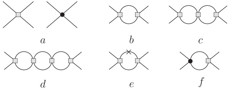
Figure 1: Diagrams contributing to the non-relativistic scattering amplitude $\mathcal{T}(p_{1}^{\prime},p_{2}^{\prime};p_{1},p_{2})$ up to and including $O(p^{3})$. The shaded squares stand for vertices with the non-derivative coupling $g_{1}$, the filled circles for the vertices with derivative couplings $g_{2},g_{3}$, and the cross corresponds to the relativistic insertion ${\bf p}^{4}/(8m)$.

2.2 Loops in the two-body sector

Now, we shall explicitly demonstrate that the matching of the couplings, given in Eq. (2.1), ensures the matching of the scattering amplitudes up to and including $O({\bf p}^{3})$ (i.e., the loops that contribute to the amplitude, are automatically the same in the relativistic and non-relativistic theories). This is because additional couplings first emerge at $O({\bf p}^{4})$. All diagrams, contributing to the non-relativistic amplitude at $O({\bf p}^{3})$, are depicted in Fig. 1. Apart from the tree-level contributions, shown in Fig. 1a, at this order one has the one-, two- and three-loop diagrams with the non-derivative vertex $g_{1}$ shown in Fig. 1b,c,d, the one-loop vertex with the insertion of the relativistic correction (Fig. 1e) and the one-loop vertex with the insertion of the derivative vertices (Fig. 1f). We shall calculate all of them separately. The tree-level contribution coincides with the quantity $\mathcal{V}_{2}$ given in Eq. (11):

$$\mathcal{T}_{2}^{(a)}=-g_{1}+4g_{2}{\bf P}^{2}+g_{3}\bigl{(}({\bf p}^{\prime}_{1}-{\bf p}^{\prime}_{2})^{2}+({\bf p}_{1}-{\bf p}_{2})^{2}\bigr{)}\,.$$ (13)

Further, using dimensional regularization, we can calculate the one-loop diagram in Fig. 1b:

$$\mathcal{T}_{2}^{(b)} = \frac{1}{2}\,g_{1}^{2}\int\frac{d^{D}l}{(2\pi)^{D}i}\,\frac{1}{\biggl{(}m-l^{0}+\dfrac{{\bf l}^{2}}{2m}-i\varepsilon\biggr{)}\biggl{(}m-P^{0}+l^{0}+\dfrac{({\bf P}-{\bf l})^{2}}{2m}-i\varepsilon\biggr{)}}$$ (14)

$$= \frac{img_{1}^{2}}{8\pi}\,\tilde{q}_{0}\,,$$

where $P_{\mu}=(p_{1}+p_{2})_{\mu}$ is the total four-momentum of the pair and $D$ is the number of the space-time dimensions ($D\to 4$ at the end of calculations). Similarly, we have:

$$\mathcal{T}_{2}^{(c)} = -g_{1}^{3}\biggl{(}\frac{im}{8\pi}\,\tilde{q}_{0}\biggr{)}^{2}\,,$$

$$\mathcal{T}_{2}^{(d)} = g_{1}^{4}\biggl{(}\frac{im}{8\pi}\,\tilde{q}_{0}\biggr{)}^{3}\,,$$ (15)

The insertion of the relativistic correction in the internal line gives:

$$\mathcal{T}_{2}^{(e)} = g_{1}^{2}\int\frac{d^{D}l}{(2\pi)^{D}i}\,\frac{{\bf l}^{4}}{8m^{3}}\,\frac{1}{\biggl{(}m-l^{0}+\dfrac{{\bf l}^{2}}{2m}-i\varepsilon\biggr{)}^{2}\biggl{(}m-P^{0}+l^{0}+\dfrac{({\bf P}-{\bf l})^{2}}{2m}-i\varepsilon\biggr{)}}$$ (16)

$$= \frac{ig_{1}^{2}\tilde{q}_{0}}{64\pi m}\,\biggl{(}5\tilde{q}_{0}^{2}+\frac{5}{2}\,{\bf P}^{2}+\frac{{\bf P}^{4}}{16\tilde{q}_{0}^{2}}\biggr{)}.$$

Finally,

$$\mathcal{T}_{2}^{(f)} = -\frac{1}{2}\,g_{1}\int\frac{d^{D}l}{(2\pi)^{D}i}\,\frac{8g_{2}{\bf P}^{2}+2g_{3}(2{\bf l}-{\bf P})^{2}+g_{3}\bigl{(}({\bf p}^{\prime}_{1}-{\bf p}^{\prime}_{2})^{2}+({\bf p}_{1}-{\bf p}_{2})^{2}\bigr{)}}{\biggl{(}m-l^{0}+\dfrac{{\bf l}^{2}}{2m}-i\varepsilon\biggr{)}\biggl{(}m-P^{0}+l^{0}+\dfrac{({\bf P}-{\bf l})^{2}}{2m}-i\varepsilon\biggr{)}}$$ (17)

$$= -\frac{img_{1}\tilde{q}_{0}}{8\pi}\,\biggl{(}8g_{2}{\bf P}^{2}+8g_{3}\tilde{q}_{0}^{2}+g_{3}\bigl{(}({\bf p}^{\prime}_{1}-{\bf p}^{\prime}_{2})^{2}+({\bf p}_{1}-{\bf p}_{2})^{2}\bigr{)}\biggr{)}\,.$$

Adding everything together up to and including $O({\bf p}^{3})$, we get:

$$\mathcal{T}_{2} = -g_{1}+4g_{2}{\bf P}^{2}+8g_{3}\tilde{q}_{0}^{2}+\frac{img_{1}^{2}\tilde{q}_{0}}{8\pi}\,\biggl{(}1+\frac{5\tilde{q}_{0}^{2}}{8m^{2}}+\frac{5{\bf P}^{2}}{16m^{2}}+\frac{{\bf P}^{4}}{128m^{2}\tilde{q}_{0}^{2}}\biggr{)}$$ (18)

$$- \frac{img_{1}\tilde{q}_{0}}{\pi}\,\biggl{(}g_{2}{\bf P}^{2}+2g_{3}\tilde{q}_{0}^{2}\biggr{)}-g_{1}^{3}\biggl{(}\frac{im}{8\pi}\,\tilde{q}_{0}\biggr{)}^{2}+g_{1}^{4}\biggl{(}\frac{im}{8\pi}\,\tilde{q}_{0}\biggr{)}^{3}\,.$$

Now, let us expand the quantity relativistic amplitude up to and including $O({\bf p}^{3})$:

$$\frac{\mathcal{M}_{2}}{4(w_{1}^{\prime}w_{2}^{\prime}w_{1}w_{2})^{1/2}}=\frac{-16\pi a_{0}\sqrt{s}}{4(w_{1}^{\prime}w_{2}^{\prime}w_{1}w_{2})^{1/2}}\biggl{(}1-ika_{0}+(ika_{0})^{2}-(ika_{0})^{3}+\frac{a_{0}r_{0}}{2}\,k^{2}-ia_{0}^{2}r_{0}k^{3}\biggr{)}\,.$$

Taking into account the relation between the quantities $k^{2}$ and $\tilde{q}_{0}^{2}$, which is given by Eq. (7), one can finally verify that the expansion of the expression in Eq. (2.2) exactly coincides with Eq. (18) term by term. This is a nice check of the matching procedure, carried out in a moving frame and including leading-order relativistic corrections.

2.3 Matching in the three-particle sector

At the order we are working, it suffices to include a single operator that describes the short-range non-derivative three-particle interactions. Note also that the coupling $\eta_{3}$ should be ultraviolet divergent in order to cancel the divergences emerging from the loops. When the dimensional regularization is used, then $\eta_{3}$ contains the term proportional to $(D-4)^{-1}$ and a finite piece. The matching condition that allows one to determine this finite piece, is given by:

$$\mathcal{T}_{3}=\prod_{i=1}^{3}\frac{1}{(2w^{\prime}_{i})^{1/2}}\,\mathcal{M}_{3}\prod_{i=1}^{3}\frac{1}{(2w_{i})^{1/2}}\,,$$ (20)

Again, both left- and right-hand sides of the above equation contain non-polynomial contributions, which should be separated before the matching for the regular part is carried out. In the two-particle case, one has achieved this goal by rewriting the matching condition in terms of the $K$-matrix, which does not contain non-polynomial contributions at all. Here, the situation is more complicated. It is important to realize that there is a certain ambiguity in the definition of the regular part of the three-body amplitude at threshold, in contrast to the two-body sector, where the parameterization of the amplitude through the effective-range expansion is commonly accepted. Below, we give a simple prescription that operates on the on-shell amplitudes only. The advantage of this prescription is that such amplitudes are physical observables that can be defined both in relativistic and non-relativistic theories.

One should also note here that, once the relation between $\eta_{3}$ and the threshold amplitude is established, one can use either of these in the fit of the three-particle energy levels. From this point of view, the matching procedure described below is superfluous. Still, we shall present it here in order to shed light on the physical meaning of the three-body coupling $\eta_{3}$ (a three-body force, in the terminology of the non-relativistic scattering theory).

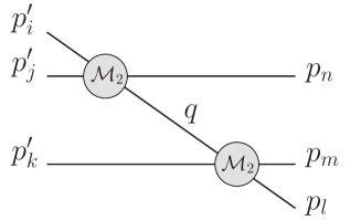
Figure 2: The most singular contribution to the relativistic three-body scattering amplitude. The four-momentum $q=p_{i}^{\prime}+p_{j}^{\prime}-p_{n}$.

Let us start by identifying the most singular piece in the relativistic amplitude. It is given by the (infinite) sum of all one-particle reducible diagrams, shown in Fig. 2. In total, there are 9 diagrams of this type, differing by permutations of the initial $p_{l},p_{m},p_{n}$ and final $p_{i}^{\prime},p_{j}^{\prime},p_{k}^{\prime}$ momenta. The contribution of all such diagrams can be written down in the following form:

$${\cal M}_{3}^{1PI}(p_{1}^{\prime},p_{2}^{\prime},p_{3}^{\prime};p_{1},p_{2},p_{3})=\sum_{(ijk)}\sum_{(lmn)}\frac{{\cal M}_{2}(p_{i}^{\prime},p_{j}^{\prime};p_{n},q){\cal M}_{2}(p_{k}^{\prime},q;p_{l},p_{m})}{m^{2}-q^{2}-i\varepsilon}\,.$$ (21)

The two-body scattering amplitude, ${\cal M}_{2}$, entering the above expression depend on three four momenta as $q=p_{i}^{\prime}+p_{j}^{\prime}-p_{n}=p_{l}+p_{m}-p_{k}^{\prime}$. These amplitudes are in general off-mass-shell, since $(p_{i}^{\prime}+p_{j}^{\prime}-p_{n})^{2}\neq m^{2}$ and $(p_{l}+p_{m}-p_{k}^{\prime})^{2}\neq m^{2}$. However, the singular contribution at $q^{2}=m^{2}$ contains only on-shell amplitudes. In order to define the on-mass-shell amplitudes, say, for the first amplitude in the numerator of Eq. (21) we perform a Lorentz boost to the center-of-mass (CM) frame of $p_{i}^{\prime},p_{j}^{\prime}$ and denote the boosted momenta ${p_{i}^{\prime}}^{*},{p_{j}^{\prime}}^{*},{p_{n}}^{*}$ and ${q}^{*}={p_{i}^{\prime}}^{*}+{p_{j}^{\prime}}^{*}-{p_{n}}^{*}$. In this frame, the amplitude depends of four variables. Two of them are related to the total energy in the initial and final state:

$$s = 4\bigl{(}({{\bf p}_{n}}^{*})^{2}+m^{2}\bigr{)}\,,$$

$$s^{\prime} = 4\bigl{(}({{\bf p}_{i}^{\prime}}^{*})^{2}+m^{2}\bigr{)}=4\bigl{(}({{\bf p}_{j}^{\prime}}^{*})^{2}+m^{2}\bigr{)}=(p_{i}^{\prime}+p_{j}^{\prime})^{2}\,,$$ (22)

and two are unit vectors:

$${\bf n}^{*}=\frac{{{\bf p}_{n}}^{*}}{|{{\bf p}_{n}}^{*}|}\,,\quad\quad{{\bf n}^{\prime}}^{*}=\frac{{{\bf p}_{i}^{\prime}}^{*}}{|{{\bf p}_{i}^{\prime}}^{*}|}=-\frac{{{\bf p}_{j}^{\prime}}^{*}}{|{{\bf p}_{j}^{\prime}}^{*}|},$$ (23)

The partial-wave expansion of the two-body amplitude takes the form:

$${\cal M}_{2}({p_{i}^{\prime}}^{*},{p_{j}^{\prime}}^{*};{p_{n}}^{*},{q}^{*})=4\pi\sum_{\ell m}Y_{\ell m}({{\bf n}^{\prime}}^{*}){\cal M}_{2}^{\ell}(s^{\prime},s)Y^{*}_{\ell m}({{\bf n}}^{*})\,.$$ (24)

The on-shell two-body amplitude is then defined at $s=s^{\prime}$:

$$\overline{{\cal M}}_{2}({p_{i}^{\prime}}^{*},{p_{j}^{\prime}}^{*};{p_{n}}^{*},{q}^{*})=4\pi\sum_{\ell m}Y_{\ell m}({{\bf n}^{\prime}}^{*}){\cal M}_{2}^{\ell}(s^{\prime},s^{\prime})Y^{*}_{\ell m}({{\bf n}}^{*})\,.$$ (25)

The second amplitude in the numerator of Eq. (21) can be treated similarly. It is evaluated at $s=(p_{l}+p_{m})^{2}$.

Finally, taking into account the identity

$$\frac{1}{m^{2}-q^{2}}=\frac{1}{2w({\bf q})}\,\biggl{\{}\frac{1}{w({\bf q})+w({\bf p}_{n})-w({\bf p}_{i}^{\prime})-w({\bf p}_{j}^{\prime})}+\frac{1}{w({\bf q})-w({\bf p}_{n})+w({\bf p}_{i}^{\prime})+w({\bf p}_{j}^{\prime})}\biggr{\}}\,,$$

where only the first term is singular, one could finally define the most singular (pole) piece of the three-body amplitude as:

$${\cal M}_{3}^{(pole)}(p_{1}^{\prime},p_{2}^{\prime},p_{3}^{\prime};p_{1},p_{2},p_{3})=\sum_{(ijk)}\sum_{(lmn)}\frac{\overline{{\cal M}}_{2}({p_{i}^{\prime}}^{*},{p_{j}^{\prime}}^{*};{p_{n}}^{*},{q}^{*})\overline{{\cal M}}_{2}({p_{k}^{\prime}}^{*},{q}^{*};{p_{l}}^{*},{p_{m}}^{*})}{2w({\bf q})(w({\bf q})+w({\bf p}_{n})-w({\bf p}_{i}^{\prime})-w({\bf p}_{j}^{\prime}))}\,.$$

The advantage of this definition is that the singular part is defined solely in terms of the observable on-shell two-body amplitudes. Note also that at the order we are working, it suffices to retain only the $S$-wave contribution in the partial-wave expansion, Eq. (24). Consequently, the numerator in Eq. (2.3) simplifies to ${\cal M}_{2}(s^{\prime}){\cal M}_{2}(s)$, with the on-shell $S$-wave amplitudes given in Eq. (4).

The difference ${\cal M}_{3}-{\cal M}_{3}^{(pole)}$ is still singular. Moreover, the singularity depends on the configuration of the initial and final three-momenta. In order to define the threshold amplitude in general, one should first perform the partial-wave expansion and then consider the limit where the magnitudes of external momenta tend to zero. However, to invoke such a cumbersome framework for matching a single coupling $\eta_{3}$ seems to be an overkill, since this goal can be achieved much easier. For example, we could agree to perform the limit ${\bf p}\to 0$ for a particular configuration of the initial and final momenta. Namely, let ${\bf e}_{x},{\bf e}_{y},{\bf e}_{z}$ denote unit vectors in the direction of axes in the momentum space. Then, choose the configuration, for example, as:

$$\begin{array}[]{l}{\bf p}_{1}=\lambda{\bf e}_{y}\,,\\[5.69054pt] {\bf p}_{2}=\lambda\biggl{(}\dfrac{\sqrt{3}}{2}\,{\bf e}_{x}-\dfrac{1}{2}\,{\bf e}_{y}\biggr{)}\,,\\[5.69054pt] {\bf p}_{3}=-\lambda\biggl{(}\dfrac{\sqrt{3}}{2}\,{\bf e}_{x}+\dfrac{1}{2}\,{\bf e}_{y}\biggr{)}\,,\end{array}$$ (31)

and ${\bf p}_{i}=-{\bf p}^{\prime}_{i}$. This means that

$${\bf p}_{k}{\bf p}_{n}={\bf p}_{k}^{\prime}{\bf p}_{n}^{\prime}=-{\bf p}^{\prime}_{k}{\bf p}_{n}=-\frac{1}{2}\lambda^{2}+\frac{3}{2}\lambda^{2}\delta_{kn},$$ (32)

For this configuration of momenta, both ${\cal M}_{3}$ and ${\cal M}_{3}^{(pole)}$ become functions of a single variable $\lambda$. In the vicinity of the three-particle threshold, their difference can be expanded in a Lorraine series:

$$\mbox{Re}\,\biggl{(}{\cal M}_{3}(\lambda)-{\cal M}_{3}^{(pole)}(\lambda)\biggr{)}=\frac{1}{\lambda}\,{\cal M}_{3}^{(-1)}+\ln\frac{\lambda}{m}\,{\cal M}_{3}^{(l)}+{\cal M}_{3}^{(0)}+\cdots\,,$$ (33)

where ellipses stand for the terms that vanish as $\lambda\to 0$, and hence do not contribute to the matching condition at threshold at this order. Here, we have arbitrarily chosen $m$ to be a scale appearing in the logarithm. Any other choice would change the definition of the regular part of the threshold amplitude ${\cal M}_{3}^{(0)}$ by an additive contribution. Note also that ${\cal M}_{3}^{(pole)}(\lambda)$ behaves like $\lambda^{-2}$ near threshold. Thus, the subtraction of the pole part indeed eliminates the leading singularity in the relativistic three-particle amplitude.

Next, we turn to the non-relativistic amplitude and carry out an extraction of the singular pieces in a similar fashion. It is important to note that if the dimensional regularization is used, only a finite number of diagrams, shown in Fig. 3, will contribute to the regular part of the threshold amplitude. In the following, we shall examine all these diagrams one by one.

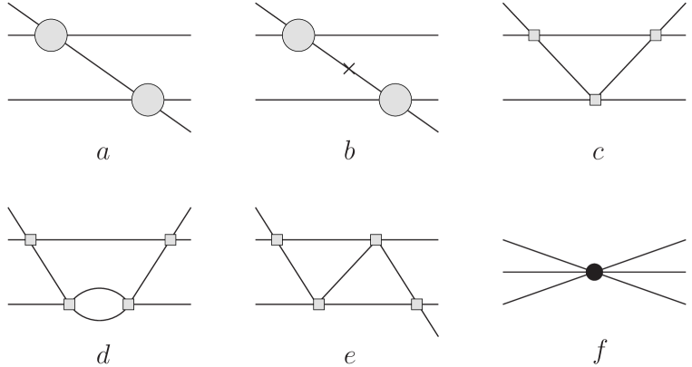
Figure 3: Diagrams that contribute to the non-vanishing three-particle scattering amplitude at threshold. The large shaded blobs in the diagram a depict the two-body scattering amplitude at $O({\bf p}^{2})$, the shaded squares correspond to the vertices with the non-derivative coupling $g_{1}$, the cross in the diagram b depicts the relativistic insertion ${\bf p}^{4}/(8m)$, and the large filled circle in the diagram f corresponds to the three-particle coupling $\eta_{3}$.

2.3.1 Singular diagrams in the non-relativistic theory

We start from the diagrams Fig. 3a and Fig. 3b. In fact, one could resum all relativistic insertions in the internal line—this obviously results in replacing the non-relativistic energies in the energy denominator by their relativistic counterparts. Thus, we get:

$$\mathcal{T}_{3}^{(a)}+\mathcal{T}_{3}^{(b)}=\sum_{\text{perm}(ijk)}\sum_{\text{perm}(lmn)}\frac{\mathcal{T}_{2}({\bf p}^{\prime}_{i},{\bf p}^{\prime}_{j};{\bf p}_{n},{\bf q})\mathcal{T}_{2}({\bf p}^{\prime}_{k},{\bf q};{\bf p}_{l},{\bf p}_{m})}{w({\bf q})-w({\bf p}^{\prime}_{i})-w({\bf p}^{\prime}_{j})+w({\bf p}_{n})-i\varepsilon}\,$$ (34)

where ${\bf q}={\bf p}^{\prime}_{i}+{\bf p}^{\prime}_{j}-{\bf p}_{n}={\bf p}_{l}+{\bf p}_{m}-{\bf p}^{\prime}_{k}$. The calculations are performed in the CM frame of three particles, i.e., ${\bf p}^{\prime}_{1}+{\bf p}^{\prime}_{2}+{\bf p}^{\prime}_{3}={\bf p}_{1}+{\bf p}_{2}+{\bf p}_{3}=0$. The quantity $\mathcal{T}_{2}$ denotes the two-point amplitude in this particular kinematics. For our purposes, it suffices to evaluate this amplitude at order ${\bf p}^{2}$, since the higher-order terms will lead to the contributions that vanish at threshold (we remind the reader that the denominator in the above equation is of order ${\bf p}^{2}$). Using Eq. (18) at this order, we get:

$$\mathcal{T}_{2}({\bf p}^{\prime}_{i},{\bf p}^{\prime}_{j};{\bf p}_{n},{\bf q}) = -g_{1}+4g_{2}{\bf P}^{2}+g_{3}\bigl{(}({\bf p}^{\prime}_{i}-{\bf p}^{\prime}_{j})^{2}+({\bf p}_{n}-{\bf q})^{2}\bigr{)}$$ (35)

$$+ i\frac{mg_{1}^{2}}{8\pi}\,q^{\prime}_{ij}+\frac{m^{2}g_{1}^{3}}{64\pi^{2}}\,(q^{\prime}_{ij})^{2}+O({\bf p}^{3})\,,$$

where

$$(q^{\prime}_{ij})^{2}=\frac{s^{\prime}_{ij}}{4}-m^{2}\,,\quad\quad s^{\prime}_{ij}=(w({\bf p}^{\prime}_{i})+w({\bf p}^{\prime}_{j}))^{2}-({\bf p}^{\prime}_{i}+{\bf p}^{\prime}_{j})^{2}\,.$$ (36)

The amplitude $\mathcal{T}_{2}({\bf p}^{\prime}_{k},{\bf q};{\bf p}_{l},{\bf p}_{m})$ is defined in a similar way.

The one-loop diagram, shown in Fig. 3c, is given by

$$\mathcal{T}_{3}^{(c)} = -g_{1}^{3}\sum_{\text{perm}(ijk)}\sum_{\text{perm}(lmn)}\int\frac{d^{D}q}{(2\pi)^{D}i}\,\frac{1}{m-q^{0}+\dfrac{{\bf q}^{2}}{2m}-i\varepsilon}$$ (37)

$$\times \frac{1}{m-{p^{\prime}_{i}}^{0}-{p^{\prime}_{j}}^{0}+q^{0}+\dfrac{({\bf p}^{\prime}_{i}+{\bf p}^{\prime}_{j}-{\bf q})^{2}}{2m}-i\varepsilon}$$

$$\times \frac{1}{m-p_{l}^{0}-p_{m}^{0}+q^{0}+\dfrac{({\bf p}_{l}+{\bf p}_{m}-{\bf q})^{2}}{2m}-i\varepsilon}\,.$$

whereas the two-loop diagrams in Fig. 3d,e take the following form:

$$\mathcal{T}_{3}^{(d)} = \frac{1}{2}\,g_{1}^{4}\sum_{\text{perm}(ijk)}\sum_{\text{perm}(lmn)}\int\frac{d^{D}q}{(2\pi)^{D}i}\,\int\frac{d^{D}k}{(2\pi)^{D}i}\,\frac{1}{m-q^{0}+\dfrac{{\bf q}^{2}}{2m}-i\varepsilon}$$ (38)

$$\times \frac{1}{m-{p^{\prime}_{i}}^{0}-{p^{\prime}_{j}}^{0}+q^{0}+\dfrac{({\bf p}^{\prime}_{i}+{\bf p}^{\prime}_{j}-{\bf q})^{2}}{2m}-i\varepsilon}$$

$$\times \frac{1}{m-p_{l}^{0}-p_{m}^{0}+q^{0}+\dfrac{({\bf p}_{l}+{\bf p}_{m}-{\bf q})^{2}}{2m}-i\varepsilon}\,\frac{1}{m-k^{0}+\dfrac{{\bf k}^{2}}{2m}-i\varepsilon}$$

$$\times \frac{1}{m-p_{l}^{0}-p_{m}^{0}-p_{n}^{0}+q^{0}+k^{0}+\dfrac{({\bf p}_{l}+{\bf p}_{m}+{\bf p}_{n}-{\bf q}-{\bf k})^{2}}{2m}-i\varepsilon}\,,$$

and

$$\mathcal{T}_{3}^{(e)} = g_{1}^{4}\sum_{\text{perm}(ijk)}\sum_{\text{perm}(lmn)}\int\frac{d^{D}q}{(2\pi)^{D}i}\,\int\frac{d^{D}k}{(2\pi)^{D}i}\,\frac{1}{m-q^{0}+\dfrac{{\bf q}^{2}}{2m}-i\varepsilon}$$ (39)

$$\times \frac{1}{m-{p^{\prime}_{i}}^{0}-{p^{\prime}_{j}}^{0}+q^{0}+\dfrac{({\bf p}^{\prime}_{i}+{\bf p}^{\prime}_{j}-{\bf q})^{2}}{2m}-i\varepsilon}$$

$$\times \frac{1}{m-p_{l}^{0}-p_{m}^{0}+k^{0}+\dfrac{({\bf p}_{l}+{\bf p}_{m}-{\bf k})^{2}}{2m}-i\varepsilon}\,\frac{1}{m-k^{0}+\dfrac{{\bf k}^{2}}{2m}-i\varepsilon}$$

$$\times \frac{1}{m-p_{l}^{0}-p_{m}^{0}-p_{n}^{0}+q^{0}+k^{0}+\dfrac{({\bf p}_{l}+{\bf p}_{m}+{\bf p}_{n}-{\bf q}-{\bf k})^{2}}{2m}-i\varepsilon}\,.$$

Finally, the diagram in Fig. 3f gives:

$$\mathcal{T}_{3}^{(f)}=-6\eta_{3}\,.$$ (40)

2.3.2 Evaluation of the singular diagrams

We start with the diagrams in Fig. 3a,b. As already mentioned, there is a subtlety here, which consists in the fact that $\mathcal{T}_{2}$, given by Eq. (35) is not on shell, i.e., $w({\bf p}^{\prime}_{i})+w({\bf p}^{\prime}_{j})\neq w({\bf p}_{n})+w({\bf q})$. For the on-shell amplitude, the Mandelstam variable $s=(p^{\prime}_{i}+p^{\prime}_{j})^{2}$. Since both particles $i,j$ are on the mass shell, we get also $s=4m^{2}+({\bf p}^{\prime}_{i}-{\bf p}^{\prime}_{j})^{2}$, but $s\neq 4m^{2}+({\bf p}_{n}-{\bf q})^{2}$. Thus, the on-shell amplitude is given by:

$$\bar{\mathcal{T}}_{2}({\bf p}^{\prime}_{i},{\bf p}^{\prime}_{j};{\bf p}_{n},{\bf q}) = -g_{1}+4g_{2}{\bf P}^{2}+2g_{3}({\bf p}^{\prime}_{i}-{\bf p}^{\prime}_{j})^{2}$$ (41)

$$+ i\frac{mg_{1}^{2}}{8\pi}\,q^{\prime}_{ij}+\frac{m^{2}g_{1}^{3}}{64\pi^{2}}\,(q^{\prime}_{ij})^{2}+O({\bf p}^{3})=\mathcal{T}_{2}+\delta\mathcal{T}_{2}\,,$$

where

$$\delta\mathcal{T}_{2}=g_{3}\bigl{(}({\bf p}^{\prime}_{i}-{\bf p}^{\prime}_{j})^{2}-({\bf p}_{n}-{\bf q})^{2}\bigr{)}\,.$$ (42)

For the second amplitude, we have the similar expression.

Further, in the matching condition, we have the factor $\bigl{(}w({\bf p}^{\prime}_{i})w({\bf p}^{\prime}_{j})\bigr{)}^{1/2}$ for the outgoing particles and the similar factor for the ingoing particles. In the off-shell kinematics, the second factor will not be equal to $\bigl{(}w({\bf p}_{n})w({\bf q})\bigr{)}^{1/2}$ anymore. Our aim is to establish, which factor should be present here. To this end, let us start from the outgoing state. In the CM frame of the pair $(i,j)$, the above factor is replaced by $\bigl{(}w({\bf p}^{\prime})w(-{\bf p}^{\prime})\bigr{)}^{1/2}$, where ${\bf p}^{\prime}$ is the relative momentum of the pair. Performing now the boost to the frame where the total momentum of the pair is ${\bf P}^{\prime}_{ij}={\bf p}^{\prime}_{i}+{\bf p}^{\prime}_{j}$, we get

$$w({\bf p}^{\prime}_{i}) = \sqrt{1-v^{2}}\bigl{(}w({\bf p}^{\prime})+v({\bf p}^{\prime}{\bf u})\bigr{)}\,,$$

$$w({\bf p}^{\prime}_{j}) = \sqrt{1-v^{2}}\bigl{(}w(-{\bf p}^{\prime})-v({\bf p}^{\prime}{\bf u})\bigr{)}\,,$$

$$v = \frac{|{\bf P}^{\prime}_{ij}|}{\sqrt{s+{{\bf P}^{\prime}_{ij}}^{2}}}\,,$$ (43)

where ${\bf u}$ denotes the unit vector in the direction of ${\bf P}^{\prime}_{ij}$.

Let now the initial pair have the relative momentum ${\bf p}$ on shell that means that $|{\bf p}^{\prime}|=|{\bf p}|$, but the direction can be arbitrary. Consequently, under the Lorentz transformation,

$$w({\bf p})\to\bar{w}_{1} = \sqrt{1-v^{2}}\bigl{(}w({\bf p})+v({\bf p}\,{\bf u})\bigr{)}\,,$$

$$w(-{\bf p})\to\bar{w}_{2} = \sqrt{1-v^{2}}\bigl{(}w(-{\bf p})-v({\bf p}\,{\bf u})\bigr{)}\,.$$ (44)

Taking into account that we are dealing with the identical particles, i.e., $w({\bf p})w(-{\bf p})$, we finally get:

$$w({\bf p}^{\prime}_{i})w({\bf p}^{\prime}_{j})-\bar{w}_{1}\bar{w}_{2}=v^{2}({\bf p}^{\prime}{\bf u})^{2}-v^{2}({\bf p}{\bf u})^{2}=O({\bf p}^{4})\,,$$ (45)

since $v^{2}=O({\bf p}^{2})$.

The brief summary of this a bit lengthy discussion is simple: at $O({\bf p}^{2})$, the matching condition for the on-shell amplitudes looks as follows

$$\bar{\mathcal{T}}_{2}({\bf p}^{\prime}_{i},{\bf p}^{\prime}_{j};{\bf p}_{n},{\bf q})=\frac{1}{2\bigl{(}w({\bf p}^{\prime}_{i})w({\bf p}^{\prime}_{j})\bigr{)}^{1/2}}\,\mathcal{M}_{2}(s^{\prime}_{ij})\frac{1}{2(\bar{w}_{1}\bar{w}_{2})^{1/2}}=\frac{\mathcal{M}_{2}(s^{\prime}_{ij})}{4w({\bf p}^{\prime}_{i})w({\bf p}^{\prime}_{j})}\,.$$ (46)

Now, the evaluation of the finite part in $\mathcal{T}_{3}^{(a)}+\mathcal{T}_{3}^{(b)}$ is straightforward:

$$\mathcal{T}_{3}^{(a)}+\mathcal{T}_{3}^{(b)}=\bar{\mathcal{T}}_{3}^{(a+b)}-\sum_{\text{perm}(ijk)}\sum_{\text{perm}(lmn)}\frac{\bar{\mathcal{T}}^{\prime}_{2}\delta\mathcal{T}_{2}+\delta\mathcal{T}^{\prime}_{2}\bar{\mathcal{T}}_{2}+\bar{\mathcal{T}}^{\prime}_{2}\bar{\mathcal{T}}_{2}(F-1)}{w({\bf q})-w({\bf p}^{\prime}_{i})-w({\bf p}^{\prime}_{j})+w({\bf p}_{n})-i\varepsilon}\,,$$ (47)

where

$$\bar{\mathcal{T}}_{3}^{(a+b)} = \prod_{i=1}^{3}\frac{1}{(2w^{\prime}_{i})^{1/2}}\,\prod_{i=1}^{3}\frac{1}{(2w_{i})^{1/2}}$$ (48)

$$\times \biggl{(}\sum_{\text{perm}(ijk)}\sum_{\text{perm}(lmn)}\frac{\mathcal{M}_{2}(s^{\prime}_{ij})\mathcal{M}_{2}(s_{lm})}{2w({\bf q})(w({\bf q})-w({\bf p}^{\prime}_{i})-w({\bf p}^{\prime}_{j})+w({\bf p}_{n})-i\varepsilon)}\biggr{)}\,,$$

and

$$F=\frac{(w({\bf p}^{\prime}_{i})w({\bf p}^{\prime}_{j}))^{1/2}}{(w({\bf p}_{n})w({\bf q}))^{1/2}}\,\frac{(w({\bf p}_{l})w({\bf p}_{m}))^{1/2}}{(w({\bf p}^{\prime}_{k})w({\bf q}))^{1/2}}\,.$$ (49)

The second term in Eq. (47) can be simplified by expanding both the numerator and denominator in momenta. The denominator cancels, and we get:

$$\mathcal{T}_{3}^{a}+\mathcal{T}_{3}^{(b)}-\bar{\mathcal{T}}_{3}^{(a+b)} = -72mg_{1}g_{3}+\frac{9g_{1}^{2}}{m}+\cdots$$ (50)

$$= \frac{288\pi^{2}a_{0}^{3}}{m}\,\biggl{(}-\frac{1}{a_{0}m^{2}}+r_{0}\biggr{)}+\frac{576\pi^{2}a_{0}^{2}}{m^{3}}+\cdots\,,$$

As one sees, the difference is a regular function at threshold, albeit both ${\cal T}_{3}^{a}+{\cal T}_{3}^{(b)}$ and $\bar{\cal T}_{3}^{(a+b)}$ scale as $1/\lambda^{2}$ at small momenta.

The rest of calculations is straightforward, because one can consider non-relativistic two-body amplitudes at $O({\bf p}^{0})$ (i.e., replace these with the scattering length). The diagram in Fig. 3c is ultraviolet-finite in the dimensional regularization. Its explicit expression is not needed. It suffices to note that, in a given configuration of external momenta,

$$\mbox{Re }{\cal T}_{3}^{(c)}=\frac{\mbox{const}}{\lambda}\,,$$ (51)

so that the constant piece is absent. Further, the diagrams in Fig. 3d,e are ultraviolet-divergent:

$$\begin{split}\mbox{Re }\mathcal{T}_{3}^{(d)}&=9\sqrt{3}g_{1}^{4}m^{3}\biggl{(}L_{2}+\frac{1}{(4\pi)^{3}}\,\ln\frac{\lambda^{2}}{m^{2}}+\frac{\delta^{(d)}}{(4\pi)^{3}}\biggr{)}\,=9\sqrt{3}g_{1}^{4}m^{3}L_{2}+\mbox{Re }\bar{\mathcal{T}}_{3}^{(d)},\\ \mbox{Re }\mathcal{T}_{3}^{(e)}&=-9\frac{4\pi}{3}\,g_{1}^{4}m^{3}\biggl{(}L_{2}+\frac{1}{(4\pi)^{3}}\,\ln\frac{\lambda^{2}}{m^{2}}+\frac{\delta^{(e)}}{(4\pi)^{3}}\biggr{)}\,=-9\,\frac{4\pi}{3}\,g_{1}^{4}m^{3}L_{2}+\mbox{Re }\bar{\mathcal{T}}_{3}^{(e)},\end{split}$$ (52)

where

$$L_{2}=\frac{(\mu^{2})^{D-4}}{(4\pi)^{3}}\,\biggl{(}\frac{1}{D-4}-\Gamma^{\prime}(1)-\ln 4\pi+\ln\frac{m^{2}}{\mu^{2}}\biggr{)}\,,$$ (53)

$\mu$ denotes the scale of the dimensional regularization, and factor 9 comes from summing all permutations. The finite parts of the above diagrams $\delta^{(d)},\delta^{(e)}$ are pure numbers, given by the integrals over Feynman parameters, see Appendix A.

Using now the matching condition for the coupling $g_{1}$, it can be seen that the three-body coupling should contain the following divergent part that cancels the divergences from the loops:

$$\eta_{3}=\frac{32\pi a_{0}^{4}}{m}\,(3\sqrt{3}-4\pi)(\mu^{2})^{D-4}\biggl{(}\frac{1}{D-4}-\Gamma^{\prime}(1)-\ln 4\pi\biggr{)}+\eta_{3}^{r}(\mu)\,,$$ (54)

with $\eta_{3}^{r}(\mu)$ being the renormalized coupling. Choosing, for simplicity, the scale $\mu=m$ in this low energy constant, we may rewrite the matching condition as:

$$-6\eta_{3}^{r}(m)=-\frac{288\pi^{2}a_{0}^{3}}{m}\,\biggl{(}-\frac{1}{a_{0}m^{2}}+r_{0}\biggr{)}-\frac{576\pi^{2}a_{0}^{2}}{m^{3}}+\bar{\mathcal{T}}\,,$$ (55)

whereas at an arbitrary scale

$$\eta_{3}^{r}(\mu)=\eta_{3}^{r}(m)-\frac{32\pi a_{0}^{4}}{m}\,(4\pi-3\sqrt{3})\,\ln\frac{m^{2}}{\mu^{2}}\,.$$ (56)

Here, the threshold amplitude $\bar{\cal T}$ is defined as:

$$\bar{\mathcal{T}}=\lim_{\lambda\to 0}\mbox{Re}\,\biggl{(}\prod_{i=1}^{3}\frac{1}{(2w^{\prime}_{i})^{1/2}}\,\mathcal{M}_{3}\prod_{i=1}^{3}\frac{1}{(2w_{i})^{1/2}}-\bar{\mathcal{T}}_{3}^{(a+b)}-\mathcal{T}_{3}^{(c)}-\bar{\mathcal{T}}_{3}^{(d)}-\bar{\mathcal{T}}_{3}^{(e)}\biggr{)}\,.$$ (57)

Finally, using Eq. (33), one may express $\bar{\mathcal{T}}$ through the relativistic threshold amplitude:

$$\bar{\mathcal{T}}=\frac{1}{(2m)^{3}}\,{\cal M}_{3}^{(0)}-\frac{192\pi a_{0}^{4}}{m}\,(3\sqrt{3}\delta^{(d)}-4\pi\delta^{(e)})\,,$$ (58)

with $\delta^{(d)},\delta^{(e)}$ as in Appendix A. In principle, Eqs. (55) and (58) solve the problem completely: they express the coupling $\eta_{3}^{r}(m)$ in terms of physical observables in the two- and three-particle sectors. A non-trivial statement, which is implicit in these equations is that threshold singularities of the three-particle amplitude are produced by two-body rescattering processes only—that is, by subtracting diagrams that describe exactly these processes, one has to arrive at a non-singular expression. Mathematically, this is equivalent to the statement that the limit $\lambda\to 0$ in Eq. (57) exists.

3 Energy shifts in the ground and excited states

In this section, we aim to derive energy shifts of the ground and excited states of multiparticle systems. Following Ref. Beane:2007qr , this calculation can be easily done within the framework of Schrödinger perturbation theory.

Let us first set up the notations. The energy levels of $N$ identical particles in a free, non-relativistic theory in finite volume are given by:

$$E_{n}(\mathbf{p}_{1},\ldots,\mathbf{p}_{N})=\frac{1}{2m}\,\sum_{i=1}^{N}{\bf p}_{i}^{2}\,\quad\quad\mathbf{p}_{i}=\frac{2\pi}{L}\mathbf{n}_{i},\quad\mathbf{n}_{i}\in\mathbb{Z}^{3},$$ (59)

where $\mathbf{p}_{i}$ is the momentum of the $i$-th particle. The set $n=\{\mathbf{n}_{i}\}$ labels the unperturbed levels. For example, the ground state corresponds to $\mathbf{n}_{i}=0,~{}i=1,\ldots N$.

We shall further see that in a regime, in which $|a_{0}/L|\ll 1$, and $mL\gg 1$, the effect of the interactions on the finite-volume spectrum in the relativistic theory can be treated as a perturbation to the free non-relativistic energy levels. Using the canonical procedure, one can construct the Hamiltonian of the system from the Lagrangian density, given in Eq. (1):

$$\mathbf{H} = \mathbf{H}_{0}+\mathbf{H}_{r}+\mathbf{H}_{1}+\mathbf{H}_{2}+\mathbf{H}_{3}+\mathbf{H}_{\eta}\,,$$

$$\mathbf{H}_{X} = \int_{L}d^{3}{\bf x}\,{\cal H}_{X}({\bf x},0)\,,\quad X\equiv 0,r,1,2,3,\eta\,,$$ (60)

where the space integral is taken over a finite cube with side $L$, and

$${\cal H}_{0} = -\frac{1}{2m}\,\psi^{\dagger}\nabla^{2}\psi\,,\quad\quad{\cal H}_{r}=-\frac{1}{8m^{3}}\,\psi^{\dagger}\nabla^{4}\psi\,,\quad\quad{\cal H}_{1}=\frac{g_{1}}{4}\,(\psi^{\dagger}\psi)^{2}\,,$$

$${\cal H}_{2} = g_{2}(\psi^{\dagger}\psi^{\dagger})\nabla^{2}(\psi\psi)\,,\quad\quad{\cal H}_{3}=g_{3}\bigl{(}(\psi^{\dagger}\psi^{\dagger})(\psi{\stackrel{{\scriptstyle\leftrightarrow}}{{\nabla}}}^{2}\psi)+\mbox{h.c}\bigr{)}\,,\quad\quad{\cal H}_{\eta}=\frac{\eta_{3}}{6}\,(\psi^{\dagger}\psi)^{3}\,.\quad\quad$$ (61)

In the above expressions, $\mathbf{H}_{0}$ denotes the free Hamiltonian, whereas $\mathbf{H}_{\text{I}}=\mathbf{H}_{r}+\mathbf{H}_{1}+\mathbf{H}_{2}+\mathbf{H}_{3}+\mathbf{H}_{\eta}$ is treated as a perturbation.

In a finite volume, free fields can be expanded in a Fourier series over the creation and annihilation operators $a^{\dagger}({\bf p}),a({\bf p})$:

$$\psi({\bf x},t)=\frac{1}{L^{3}}\,\sum_{\bf p}e^{-ip^{0}t+i{\bf p}{\bf x}}a({\bf p})\,,\quad\quad\psi^{\dagger}({\bf x},t)=\frac{1}{L^{3}}\,\sum_{\bf p}e^{ip^{0}t-i{\bf p}{\bf x}}a^{\dagger}({\bf p})\,.$$ (62)

Here, the momentum ${\bf p}$ runs over discrete values ${\bf p}=2\pi{\bf n}/L\,,~{}{\bf n}\in\mathbb{Z}^{3}$, and the creation/annihilation operators obey the following commutation relations:

$$[a({\bf p}),a^{\dagger}({\bf q})]=L^{3}\delta_{{\bf p}{\bf q}}\,.$$ (63)

The properly normalized unperturbed eigenstates are given by:

$$\ket{\mathbf{p}_{1},\ldots,\mathbf{p}_{N}}=\frac{1}{\sqrt{N!}\,L^{3N/2}}\,a^{\dagger}(\mathbf{p}_{1})\ldots a^{\dagger}(\mathbf{p}_{N})\ket{0}\,.$$ (64)

These eigenstates obey the eigenvalue equation:

$$\mathbf{H}_{0}\ket{\mathbf{p}_{1},\ldots,\mathbf{p}_{N}}=E_{n}(\mathbf{p}_{1},\ldots,\mathbf{p}_{N})\ket{\mathbf{p}_{1},\ldots,\mathbf{p}_{N}}\,.$$ (65)

One may also define the matrix elements of the interaction Hamiltonian between the unperturbed states:

$$V_{qp}=\bra{\mathbf{q}_{1},\ldots,\mathbf{q}_{N}}\mathbf{H}_{\text{I}}\ket{\mathbf{p}_{1},\ldots,\mathbf{p}_{N}}\,.$$ (66)

The Rayleigh-Schrödinger perturbation theory enables one to calculate the energy shift of a state $n$ using the interaction Hamiltonian $\mathbf{H}_{\text{I}}$. A standard formula, which can be found in the quantum mechanics textbooks (see, e.g., Landau-Lifshits ), reads:

$$\Delta E_{n}=V_{nn}+\sum_{p\neq n}\frac{|V_{np}|^{2}}{E_{n}-E_{p}}+\sum_{p,q\neq n}\frac{V_{np}V_{pq}V_{qn}}{(E_{n}-E_{p})(E_{n}-E_{q})}-V_{nn}\sum_{p\neq n}\frac{|V_{np}|^{2}}{(E_{n}-E_{p})^{2}}+O(V^{4})\,.$$

Note that we decided not to display here a (rather cumbersome) fourth-order formula, which is also needed in the calculations at order $L^{-6}$.

3.1 Two-particle levels

As a warm-up example, we consider the well-known case of two particles in the center-of-mass (CM) frame. The $1/L$ expansion of the energy shift for the two-particle ground state has been known for a long time up to and including $O(L^{-5})$ Huang:1957im ; Luscher:1986n2 . At this order, the effects of relativity are irrelevant and one can work in a non-relativistic setup. The next order was worked out in the NREFT approach Beane:2007qr , and in a fully relativistic setup Hansen:2015zta ; Hansen:2016fzj . As pointed out in Ref. Hansen:2015zta , these two calculations differ by a term that vanishes in the limit $m\to\infty$, and can be referred to as “relativistic corrections”. Recently, in Ref. Beane:2020ycc , relativistic corrections to the ground state were derived in the NREFT with a method, which is identical to the one used here. Below, for illustrative purpose, we shall rederive $1/L$ expansion of the energy shift up to and including $O(L^{-6})$ by using Rayleigh-Schrödinger perturbation theory.

The matrix element to the interaction Hamiltonian between the two-particle unperturbed states is given by:

$$V_{qp}=\braket{\mathbf{q}_{1},\mathbf{q}_{2}}{\mathbf{H}_{\text{I}}}{\mathbf{p}_{1},\mathbf{p}_{2}}\,.$$ (68)

Calculating the matrix element, one gets:

$$V_{qp} = \frac{1}{2L^{3}}\left[g_{1}-g_{3}(\mathbf{q}_{1}-\mathbf{q}_{2})^{2}-g_{3}(\mathbf{p}_{1}-\mathbf{p}_{2})^{2}\right]\delta_{\mathbf{q}_{1}+\mathbf{q}_{2},\mathbf{p}_{1}+\mathbf{p}_{2}}$$ (69)

$$- \frac{1}{16m^{3}}\left[\mathbf{q}_{1}^{4}+\mathbf{q}_{2}^{4}+\mathbf{p}_{1}^{4}+\mathbf{p}_{2}^{4}\right]\,\frac{1}{2!}\,\sum_{(ij)\in\,\mathcal{S}_{2}}\delta_{\mathbf{q}_{1}\mathbf{p}_{i}}\delta_{\mathbf{q}_{2}\mathbf{p}_{j}}\,,$$

where the sum in the last term runs over the two-element permutation group $\mathcal{S}_{2}$ for the indices $i,j$. The relation between $g_{1,3}$ and $a_{0},r_{0}$ is given in Eq. (2.1). The term with $g_{2}$ does not contribute in the CM frame and is therefore omitted here.

Now, using Eq. (3), we can calculate the energy shift of the ground state order by order in perturbation theory. It is easy to verify that, at lowest order, only terms with the non-derivative coupling $g_{1}$ from the interaction Hamiltonian, $\mathbf{H}_{\text{I}}$, contribute:

$$\Delta E_{0}^{(1)}=V_{00}=\frac{g_{1}}{2L^{3}}=\frac{4\pi a_{0}}{mL^{3}}\,.$$ (70)

In order to evaluate the next-order result, we use Eq. (69) and get:

$$V_{0p}=-\frac{1}{2L^{3}}\,(g_{1}-4g_{3}{\bf p}^{2})\delta_{{\bf 0},{\bf p}_{1}+{\bf p}_{2}}\,,\quad\quad{\bf p}_{1}=-{\bf p}_{2}={\bf p}\,.$$ (71)

Substituting this expression into the second-order energy shift, Eq. (3), and using $E_{0}=0$, $E_{p}={\bf p}^{2}/m$, we get:

$$\Delta E_{0}^{(2)} = \frac{1}{4L^{6}}\,\sum_{p\neq 0}\frac{(g_{1}-4g_{3}{\bf p}^{2})^{2}}{E_{0}-E_{p}}=-\frac{g_{1}^{2}m}{16\pi^{2}L^{4}}\sum_{\mathbf{n}\neq\mathbf{0}}\frac{1}{\mathbf{n}^{2}}+\frac{2g_{1}g_{3}m}{L^{6}}\,\sum_{\mathbf{n}\neq\mathbf{0}}1+O(L^{-8})$$ (72)

$$= -\frac{4\pi a_{0}}{mL^{3}}\frac{a_{0}}{\pi L}\mathcal{I}+\frac{4\pi a_{0}}{mL^{3}}\,\frac{2\pi a_{0}^{2}}{L^{3}}\,\biggl{(}r_{0}-\frac{1}{a_{0}m^{2}}\biggr{)}+O(L^{-8})\,.$$

Here, one has used ${\bf p}=2\pi{\bf n}/L$ in order to display the powers of $L$ explicitly. It is already clear that one has a double perturbative expansion in powers of $1/L$. First, each order in Rayleigh-Schrödinger perturbation theory brings a factor $L^{-3}$ associated to the momentum sum and a factor $L^{2}$, emerging from the propagator, $L^{-1}$ in total. The pertinent expansion parameter here is $a_{0}/L$. Further, each derivative vertex is suppressed by powers of $L$, since the momentum ${\bf p}$ scales as $1/L$. In this case, the pertinent expansion parameter is $1/(mL)$. Consequently, in order to obtain an expression of the energy shift to a given order in $1/L$, it suffices to retain finite number of terms in the effective Lagrangian and truncate the perturbative series at a fixed order.

Furthermore, the momentum sums emerging in Eq. (72), are formally ultraviolet divergent. In order to be consistent with the matching condition, this divergence should be subtracted in the same way as in the infinite volume, i.e., by using the $\overline{\text{MS}}$ scheme in dimensional regularization. In this particular case, it is very simple. Namely, one might rewrite the first sum as:

$${\cal I}=\sum_{\mathbf{n}\neq\mathbf{0}}\frac{1}{\mathbf{n}^{2}}=\sum_{\mathbf{n}\neq\mathbf{0}}\frac{1}{\mathbf{n}^{2}(\mathbf{n}^{2}+1)}-1+\sum_{\mathbf{n}}\frac{1}{\mathbf{n}^{2}+1}\,.$$ (73)

Here, we have added and subtracted the term with $\mathbf{n}=\mathbf{0}$ in the last sum. Now, the first term is perfectly convergent, and the last term can be calculated by means of the Poisson summation formula, applying the $\overline{\text{MS}}$ scheme to the $|\mathbf{n}|=0$ term:

$$\sum_{\mathbf{n}}\frac{1}{\mathbf{n}^{2}+1}=\int d^{d}x\frac{1}{x^{2}+1}+\sum_{n\neq 0}\frac{\pi}{|\mathbf{n}|}e^{-2\pi|\mathbf{n}|}.$$ (74)

This way, one gets:

$${\cal I}=\sum_{\mathbf{n}\neq\mathbf{0}}\frac{1}{\mathbf{n}^{2}(\mathbf{n}^{2}+1)}-1-2\pi^{2}+\sum_{\mathbf{n}\neq\mathbf{0}}\frac{\pi}{|{\bf n}|}\,e^{-2\pi|{\bf n}|}\simeq-8.9136329.$$ (75)

Acting in the same way, one can easily see that

$$\sum_{\mathbf{n}\neq\mathbf{0}}1=-1\,,$$ (76)

and finally, using the matching condition for $g_{1,3}$, one arrives at the last line of Eq. (72).

Continuing in the same manner, one can calculate corrections up to and including order $L^{-6}$. The result is given by the following expression:

$$\Delta E_{0} = \frac{4\pi a_{0}}{mL^{3}}\Bigg{\{}1-\frac{a_{0}}{\pi L}\mathcal{I}+\left(\frac{a_{0}}{\pi L}\right)^{2}\left[\mathcal{I}^{2}-\mathcal{J}\right]-\frac{\pi a_{0}}{m^{2}L^{3}}+\frac{2\pi a_{0}^{2}r_{0}}{L^{3}}$$ (77)

$$- \left(\frac{a_{0}}{\pi L}\right)^{3}\left[\mathcal{I}^{3}-3\mathcal{I}\mathcal{J}+\mathcal{K}\right]\Bigg{\}}\,,$$

where

$$\mathcal{J}=\sum_{\mathbf{n}\neq\mathbf{0}}\frac{1}{\mathbf{n}^{4}}\simeq 16.5323\,,\quad\quad\mathcal{K}=\sum_{\mathbf{n}\neq\mathbf{0}}\frac{1}{\mathbf{n}^{6}}\simeq 8.40192.$$ (78)

This, of course, agrees with the result of Refs. Hansen:2015zta ; Hansen:2016fzj as well as Ref. Beane:2020ycc . Moreover, relativistic corrections are easy to identify. They emerge from the contributions from $\mathbf{H}_{3}$ and $\mathbf{H}_{r}$. If they are dropped, the result in Ref. Beane:2007qr is recovered.

Next, we turn to the relativistic energy shift for the first excited state in the two-particle sector. We start by defining the unperturbed states. In the non-interacting theory and for identical particles, this state is threefold degenerate in the relativistic, as well in the non-relativistic case and has unit back-to-back momentum in the units of $2\pi/L$, directed along the $x,y$ or $z$-axis. These three states can be classified in irreducible representations of the cubic group. There is a one-dimensional irrep $A_{1}^{+}$, and a two-dimensional irrep $E^{+}$. The two-particle $A^{+}_{1}$ state is given by:

$$\ket{({\bf p},-{\bf p})_{A_{1}^{+}}}=\frac{1}{\sqrt{6}}\sum_{a=x,y,z}\biggl{(}\ket{\mathbf{p}_{a},-\mathbf{p}_{a}}+\ket{-\mathbf{p}_{a},\mathbf{p}_{a}}\biggr{)},$$ (79)

where $\mathbf{p}_{x}=\dfrac{2\pi}{L}\,(1,0,0)$, and so on. The basis vectors of the irrep $E^{+}$ are given by:

$$\ket{({\bf p},-{\bf p})_{E^{+}},1} = \frac{1}{2}\biggl{(}\ket{\mathbf{p}_{x},-\mathbf{p}_{x}}+\ket{-\mathbf{p}_{x},\mathbf{p}_{x}}-\ket{\mathbf{p}_{y},-\mathbf{p}_{y}}-\ket{-\mathbf{p}_{y},\mathbf{p}_{y}}\biggr{)}\,,$$

$$\ket{({\bf p},-{\bf p})_{E^{+}},2} = \frac{1}{\sqrt{12}}\biggl{(}\ket{\mathbf{p}_{x},-\mathbf{p}_{x}}+\ket{-\mathbf{p}_{x},\mathbf{p}_{x}}+\ket{\mathbf{p}_{y},-\mathbf{p}_{y}}+\ket{-\mathbf{p}_{y},\mathbf{p}_{y}}$$ (80)

$$- 2\ket{\mathbf{p}_{z},-\mathbf{p}_{z}}-2\ket{-\mathbf{p}_{z},\mathbf{p}_{z}}\biggr{)}\,.$$

Because of the cubic symmetry, any of these two states can be used for the calculation of the energy shift.

The calculation of the energy shifts proceeds analogously to the case of ground state. We do not display the intermediate steps here. Note that the energy shifts are calculated with respect to the relativistic unperturbed energy of the first unperturbed state $\displaystyle E_{1}=2\sqrt{m^{2}+(2\pi/L)^{2}}-2m$. It is easy to see that the leading contribution to the energy shift in the irrep $E^{+}$ arises from the $D$-wave interaction and is beyond the accuracy we are calculating:

$$\Delta E_{1}^{E^{+}}=O(L^{-7}).$$ (81)

The shift in the irrep $A_{1}^{+}$ at order $L^{-5}$ was calculated in Ref. Luscher:1986n2 . In the present paper this result is extended up to and including order $L^{-6}$, where the method, used in Ref. Luscher:1986n2 , does not directly apply for the calculation of the relativistic corrections. The final answer reads:

$$\begin{split}\Delta E^{A_{1}^{+}}_{1}=\frac{24\pi a_{0}}{mL^{3}}\Bigg{\{}&1-\mathcal{I}_{1}\frac{a_{0}}{\pi L}+(\mathcal{I}_{1}^{2}-6\mathcal{J}_{1})\left(\frac{a_{0}}{\pi L}\right)^{2}+(-\mathcal{I}_{1}^{3}+18\mathcal{I}_{1}\mathcal{J}_{1}-36\mathcal{K}_{1})\left(\frac{a_{0}}{\pi L}\right)^{3}\\ &+\frac{2\pi^{2}a_{0}r_{0}}{L^{2}}\left[1-\mathcal{I}_{1}\frac{a_{0}}{\pi L}\right]-\frac{2\pi^{2}}{m^{2}L^{2}}\left[1+\frac{\mathcal{J}_{1}-1}{2}\frac{a_{0}}{\pi L}\right]\Bigg{\}}\,.\end{split}$$ (82)

Here,

$$\mathcal{I}_{1} = \sum_{|\mathbf{n}|\neq 1}\frac{1}{{\bf n}^{2}-1}\doteq\sum_{|\mathbf{n}|\neq 1}\frac{2}{(\mathbf{n}^{2}-1)(\mathbf{n}^{2}+1)}-3-2\pi^{2}+\sum_{\mathbf{n}\neq\mathbf{0}}\frac{\pi}{|{\bf n}|}\,e^{-2\pi|{\bf n}|}\simeq-1.2113357\,,$$

$$\mathcal{J}_{1} = \sum_{|\mathbf{n}|\neq 1}\frac{1}{({\bf n}^{2}-1)^{2}}\simeq 23.2432219\,,$$

$$\mathcal{K}_{1} = \sum_{|\mathbf{n}|\neq 1}\frac{1}{({\bf n}^{2}-1)^{3}}\simeq 13.0593768\,$$ (83)

3.2 Ground state of $N$ particles

If we are dealing with more than two particles, two new effects arise. First, the two-particle subsystems can be in the moving frames, even if the total momentum of the $N$-particle system vanishes. Therefore, $\mathbf{H}_{2}$ in Eq. (60) starts to contribute (still, as we will see, this contribution is only non-vanishing for excited states ). Second, one has to take into account the contribution from the non-derivative three-particle interaction, which is parameterized by the coupling constant $\eta_{3}$. Four- and more particle interactions, as well as the operators with higher derivatives in the two- and three-particle sectors do not contribute at the order we are working. In particular, from Eq. (64) it is seen that the normalization of the $N$-particle wave function depends only on $L$. Then, on dimensional grounds, a generic operator in the Lagrangian, $\delta{\cal L}=c_{k}\ \mathcal{O}_{k}$, where $c_{k}$ has the mass dimension $[c_{k}]=M^{k}$, starts to contribute to the energy shift at $\Delta E\sim c_{k}L^{k-1}$. For example, one can see that the operator of the type $(\psi\psi^{\dagger})^{N}$ contributes to order $L^{-3(N-1)}$.

The expression in Eq. (69) can be easily generalized to more than two particles. For instance, for three particles, we have:

$$V_{qp} = \sum_{k=1,2,3}\frac{1}{2L^{3}}\left[g_{1}-4g_{2}(\mathbf{q}_{i}+\mathbf{q}_{j})^{2}-g_{3}(\mathbf{q}_{i}-\mathbf{q}_{j})^{2}-g_{3}(\mathbf{p}_{i}-\mathbf{p}_{j})^{2}\right]\delta_{\mathbf{q}_{i}+\mathbf{q}_{j},\mathbf{p}_{i}+\mathbf{p}_{j}}\delta_{\mathbf{q}_{k},\mathbf{p}_{k}}$$ (84)

$$+ \frac{\eta_{3}}{L^{6}}\,\delta_{\mathbf{q}_{1}+\mathbf{q}_{2}+\mathbf{q}_{3},\mathbf{p}_{1}+\mathbf{p}_{2}+\mathbf{p}_{3}}$$

$$- \frac{1}{16m^{3}}\,\left[\mathbf{q}_{1}^{4}+\mathbf{q}_{2}^{4}+\mathbf{q}_{3}^{4}+\mathbf{p}_{1}^{4}+\mathbf{p}_{2}^{4}+\mathbf{p}_{4}^{4}\right]\,\frac{1}{3!}\,\sum_{(ijk)\,\in\,\mathcal{S}_{3}}\delta_{\mathbf{q}_{1}\mathbf{p}_{i}}\delta_{\mathbf{q}_{2}\mathbf{p}_{j}}\delta_{\mathbf{q}_{3}\mathbf{p}_{k}}\,,$$

where $i\neq j\neq k$. This expression is easy to understand. In the first line, there are three pairwise interactions, in which $k$ labels the spectator particle; the second line stems from the three-particle contact interaction; and the third line corresponds to the kinetic term at $O({\bf p}^{4})$. Note that, in this case, the indices in the last sum run over the three-element permutation group $\mathcal{S}_{3}$. For more than three particles, the generalizations are straightforward at this order and include only additional combinatorial factors. In particular, there exist $\binom{N}{2}$ pairwise interactions, $\binom{N}{3}$ three-particle interactions, and $N!$ permutations in the kinetic term.

Further, we shall take an advantage of the fact that the expression without relativistic corrections has been already derived previously exactly with the same method Beane:2007qr . The remainder can be calculated relatively easy. The final result for the $N$-particle ground state, expressed in terms of the threshold amplitude $\bar{\mathcal{T}}$, has the form:

$$\begin{split}\Delta E_{0}&=\binom{N}{2}\frac{4\pi a_{0}}{mL^{3}}\Bigg{\{}1-\frac{a_{0}}{\pi L}\mathcal{I}+\left(\frac{a_{0}}{\pi L}\right)^{2}\left[\mathcal{I}^{2}+(2N-5)\mathcal{J}\right]\\ &-\left(\frac{a_{0}}{\pi L}\right)^{3}\left[\mathcal{I}^{3}+(2N-7)\mathcal{I}\mathcal{J}+(5N^{2}-41N+63)\mathcal{K}+8(N-2)(2\mathcal{Q}+\mathcal{R})\right]\\ &+(4N-9)\frac{\pi a_{0}}{m^{2}L^{3}}+(4N-6)\frac{\pi a_{0}^{2}r_{0}}{L^{3}}\Bigg{\}}\\ &+\binom{N}{3}\Bigg{\{}\frac{32\pi a_{0}^{4}}{mL^{6}}\left(3\sqrt{3}-4\pi\right)(2\ln(mL)-\Gamma^{\prime}(1)-\ln 4\pi)-\frac{\bar{\mathcal{T}}}{6L^{6}}\Bigg{\}}\,.\end{split}$$ (85)

Here, the quantities ${\cal I},{\cal J},{\cal K}$ were defined above, whereas the quantities ${\cal Q}\simeq-102.1556055$ and ${\cal R}\simeq 19.186903$ are the quantities defined in Ref. Beane:2007qr . The factor $(\Gamma^{\prime}(1)+\ln 4\pi)$ emerges, because the quantities ${\cal Q},{\cal R}$ in Ref. Beane:2007qr are defined in the MS renormalization scheme rather than $\overline{\text{MS}}$, which is used in the present paper. Further, we confirm that the above equation agrees with Eq. (42) of Ref. Beane:2020ycc , if expressed in terms of the renormalized coupling $\eta_{3}^{r}$. In order to compare with the result of Refs. Hansen:2015zta ; Hansen:2016fzj , one has to carry out the matching of the threshold amplitude, defined in those papers, to the quantity $\bar{\mathcal{T}}$. We do not do this (rather straightforward but tedious) exercise here.

3.3 Energy shift for the three-particle excited states.

In this section we discuss the calculation of relativistic corrections to the excited state levels in the three-particle state. To the best of our knowledge, this issue has not been addressed so far in the literature and appears here for the first time. Note also that the combinatorics in the excited states becomes rather cumbersome. For this reason, we first focus on three particles.

Let us start with the definition of the state vectors. In the three-particle system in the CM frame, the first excited unperturbed state contains one particle at rest, whereas two other particles have back-to-back momenta of unit magnitude, in units of $2\pi/L$. Again, the first excited states contains only the $A_{1}^{+}$ and $E^{+}$ irreps of the cubic group. The pertinent basis functions are:

$$\ket{A_{1}^{+}} = \frac{1}{\sqrt{3}}\,\biggl{(}\ket{({\bf p}_{1},{\bf p}_{2})_{A_{1}^{+}},{\bf p}_{3}=0}+\ket{({\bf p}_{3},{\bf p}_{1})_{A_{1}^{+}},{\bf p}_{2}=0}+\ket{({\bf p}_{2},{\bf p}_{3})_{A_{1}^{+}},{\bf p}_{1}=0}\biggr{)}\,,$$

$$\ket{E^{+},\alpha} = \frac{1}{\sqrt{3}}\,\biggl{(}\ket{(({\bf p}_{1},{\bf p}_{2})_{E^{+}},\alpha),{\bf p}_{3}=0}+\ket{(({\bf p}_{3},{\bf p}_{1})_{E^{+}},\alpha),{\bf p}_{2}=0}$$ (86)

$$\hskip 142.26378pt+\ket{(({\bf p}_{2},{\bf p}_{3})_{E^{+}},\alpha),{\bf p}_{1}=0}\biggr{)}\,,$$

where $\alpha=1,2$ and the basis vectors $\ket{(p_{i},p_{j})_{A_{1}^{+}}}$ and $\ket{(p_{i},p_{j})_{E^{+}},\alpha}$ with back-to-back three-momenta ${\bf p}_{i}$ and ${\bf p}_{j}$ are given by Eqs. (79) and (3.1), respectively.

As a simple check, let us calculate the energy level shift at leading order:

$$\Delta E_{1}^{A_{1}^{+}} = \braket{A_{1}^{+}}{\mathbf{H}_{1}}{A_{1}^{+}}=\frac{40\pi a_{0}}{mL^{3}}+O(L^{-4})\,,$$

$$\Delta E_{1}^{E^{+}} = \braket{E^{+},\alpha}{\mathbf{H}_{1}}{E^{+},\alpha}=\frac{16\pi a_{0}}{mL^{3}}+O(L^{-4})\,.$$ (87)

It is seen that the leading-order result of Ref. Pang:2019dfe is readily reproduced. One might continue along the same path and evaluate all contributions up to and including $O(L^{-6})$. However, since the result in the non-relativistic limit is already known Pang:2019dfe , one can achieve the same goal with a significantly less effort, evaluating only the relativistic corrections to this result. Below we shall demonstrate, how this can be done.

Let us start from the energy shift in the irrep $E^{+}$, which does not contain the three-body coupling $\eta_{3}^{r}$. The non-relativistic result, given in Ref. Pang:2019dfe , reads:

$$\Delta E_{1}^{E^{+}}(\text{non-rel})=\frac{16\pi a_{0}}{mL^{3}}\,\biggl{(}1+\frac{h_{1}^{\prime}}{L}+\frac{h_{2}^{\prime}}{L^{2}}+\frac{h_{4}^{\prime}}{L^{3}}+\cdots\biggr{)}\,.$$ (88)

Here,

$$h_{1}^{\prime} = y_{1}^{\prime}a_{0}\,,$$

$$h_{2}^{\prime} = y_{2}^{\prime}a_{0}^{2}+\frac{\pi^{2}}{2}\,r_{0}a_{0}\,,$$

$$h_{4}^{\prime} = y_{4}^{\prime}a_{0}^{3}+\pi(11-{\cal I}_{2})r_{0}a_{0}^{2}\,,$$ (89)

where the numerical constants $y_{1}^{\prime}=2.984094$, $y_{2}^{\prime}=3.001706$, $y_{4}^{\prime}=-28.89478538$ are complicated combinations of the infinite sums. The quantity ${\cal I}_{2}$ is defined as:

$$\begin{split}{\cal I}_{2}&=\sum_{{\bf n}\neq{\bf 0},-{\bf n}_{0}}\frac{1}{{\bf n}^{2}+{\bf n}{\bf n}_{0}}\doteq\sum_{{\bf n}\neq{\bf 0},-{\bf n}_{0}}\biggl{(}\frac{1}{{\bf n}^{2}+{\bf n}{\bf n}_{0}}-\frac{1}{{\bf n}^{2}+1}\biggr{)}-\frac{3}{2}\\ &-2\pi^{2}+\sum_{\mathbf{n}\neq\mathbf{0}}\frac{\pi}{|{\bf n}|}\,e^{-2\pi|{\bf n}|}\simeq-6.37480912\,,\end{split}$$ (90)

where ${\bf n}_{0}=(0,0,1)$ is a unit vector Pang:2019dfe .

Relativistic corrections to this result emerge from three different sources:

1. shifting the effective range $r_{0}\to r_{0}-1/(a_{0}m^{2})$, according to Eq. (2.1):

   $$\Delta E_{1}^{E^{+}}(\text{eff.range})=\frac{16\pi a_{0}}{mL^{3}}\,\biggl{(}-\frac{\pi^{2}}{2m^{2}L^{2}}-\frac{\pi a_{0}}{m^{2}L^{3}}\,(11-{\cal I}_{2})\biggr{)}\,;$$ (91)

2. contributions, containing the coupling $g_{2}$, which vanishes in the non-relativistic limit. This contribution describes the CM motion of the two-particle subsystem in the three-particle system at rest:

   $$\Delta E_{1}^{E^{+}}(\text{CM}) = -\frac{32\pi^{2}}{L^{5}}\,g_{2}+\frac{8mg_{1}g_{2}}{L^{6}}\,(-3+{\cal I}_{2})$$ (92)

   $$= \frac{16\pi a_{0}}{mL^{3}}\,\biggl{(}-\frac{\pi^{2}}{m^{2}L^{2}}+\frac{2\pi a_{0}}{m^{2}L^{3}}\,({\cal I}_{2}-3)\biggr{)}\,;$$

3. contributions, emerging from the $O({\bf p}^{4})$ kinetic term $\mathbf{H}_{r}$:

   $$\Delta E_{1}^{E^{+}}(\text{kinetic})=\frac{16\pi a_{0}}{mL^{3}}\,\frac{\pi a_{0}}{2m^{2}L^{3}}\,(15-4{\cal S})\,,$$ (93)

   where

   $${\cal S} = \sum_{\mathbf{n}\neq\mathbf{0},\mathbf{n}_{0}}\frac{\mathbf{n}^{4}+(\mathbf{n}-\mathbf{n}_{0})^{4}+1}{(\mathbf{n}^{2}+(\mathbf{n}-\mathbf{n}_{0})^{2}-1)^{2}}$$ (94)

   $$= -\frac{13}{8}+\frac{1}{2}\,\sum_{\mathbf{n}\neq\mathbf{0},\mathbf{n}_{0}}(\mathbf{n}^{2}+(\mathbf{n}\mathbf{n}_{0})^{2}-2\mathbf{n}\mathbf{n}_{0}+1)\biggl{(}\frac{1}{(\mathbf{n}^{2}-\mathbf{n}\mathbf{n}_{0})^{2}}-\frac{1}{(\mathbf{n}^{2}+1)^{2}}\biggr{)}$$

   $$- \frac{1}{6}\,\sum_{\mathbf{n}}\frac{1}{(\mathbf{n}^{2}+1)^{2}}-\frac{4\pi^{2}}{3}+\sum_{\mathbf{n}\neq 0}\frac{2\pi}{3|\mathbf{n}|}\,e^{-2\pi|\mathbf{n}|}\simeq 1.849866\,.$$

Bringing everything together, we get:

$$\Delta E_{1}^{E^{+}}=\Delta E_{1}^{E^{+}}(\text{non-rel})+\Delta E_{1}^{E^{+}}(\text{rel})\,,$$ (95)

where

$$\Delta E_{1}^{E^{+}}(\text{rel})=\frac{16\pi a_{0}}{mL^{3}}\,\biggl{(}-\frac{3\pi^{2}}{2(mL)^{2}}+\frac{\pi a_{0}}{2m^{2}L^{3}}\,(-19+6{\cal I}_{2}-4{\cal S})\biggr{)}\,,$$ (96)

and $\Delta E_{1}^{E^{+}}(\text{non-rel})$ as in Eq. (88).

Next, we turn to the energy shift in the irrep $A_{1}^{+}$, which, in contrast to the $E^{+}$, contains contribution from the three-body coupling. We shall again be using a shortcut, calculating only the relativistic corrections to the result given in Ref. Pang:2019dfe . To this end, comparing first the expressions for the ground-state energy shift in the non-relativistic limit, we read off the relation between the three-body coupling $\eta_{3}^{r}(m)$ and the threshold amplitude $\hat{\cal M}$ from Ref. Pang:2019dfe :

$$\eta_{3}^{r}(m)=-\frac{96\pi^{2}a_{0}^{2}}{m}\,\hat{\cal M}+\frac{48\pi^{2}a_{0}^{3}}{m}\,r_{0}-\frac{12a_{0}^{4}}{\pi^{2}m}\,A\,,$$ (97)

where $A$ collects all numerical factors that account for the different regularization and conventions, used in Ref. Pang:2019dfe and the present article:

$$\begin{split}A&=\frac{1}{3}\,(2\pi)^{3}(3\sqrt{3}-4\pi)(2\ln 2\pi-\Gamma^{\prime}(1)-\ln 4\pi)+\pi\delta+16(\tilde{\cal Q}-{\cal Q})+8(\tilde{\cal R}-{\cal R})\\ &\simeq 1278.49567\,.\end{split}$$ (98)

Here, $\delta\simeq 887.65392$ and $\tilde{\cal Q}\simeq-105.0597779$, $\tilde{\cal R}\simeq-32.60560475$ are the counterparts of ${\cal Q},{\cal R}$ in the cutoff regularization. All these quantities have been defined in Ref. Pang:2019dfe .

Next, let us consider the expression for the energy shift of the first excited state in the $A_{1}^{+}$ irrep in the non-relativistic theory, given in Ref. Pang:2019dfe :

$$\Delta E_{1}^{A_{1}^{+}}(\text{non-rel})=\frac{40\pi a_{0}}{mL^{3}}\,\biggl{(}1+\frac{h_{1}}{L}+\frac{h_{2}}{L^{2}}+\frac{h_{3}}{L^{3}}\,\ln\frac{mL}{2\pi}+\frac{h_{4}}{L^{3}}\biggr{)}\,,$$ (99)

where

$$h_{1} = y_{1}a_{0}\,,$$

$$h_{2} = y_{2}a_{0}^{2}+\frac{7\pi^{2}}{5}\,a_{0}r_{0}\,,$$

$$h_{3} = \frac{144}{5}\,(3\sqrt{3}-4\pi)a_{0}^{3}\,,$$

$$h_{4} = y_{4}a_{0}^{3}+\frac{\pi}{10}\,a_{0}^{2}r_{0}(212-24{\cal I}_{1}-4{\cal I}_{2})-\frac{27}{5}\,8\pi a_{0}\hat{\cal M}\,,$$ (100)

where $y_{1}\simeq 0.279070$, $y_{2}\simeq 8.494802$ and $y_{4}\simeq-172.001650$ are numerical constants, defined in Ref. Pang:2019dfe . Using now the relation (97), one may rewrite last of the above equations as:

$$h_{4}=\biggl{(}y_{4}+\frac{27}{5\pi^{3}}\,A\biggr{)}a_{0}^{3}-\frac{2\pi}{5}\,a_{0}^{2}r_{0}(1+6{\cal I}_{1}+{\cal I}_{2})+\frac{9m}{20\pi a_{0}}\,\eta_{3}^{r}(m)\,.$$ (101)

Now, we can readily evaluate the relativistic corrections to this result from three different sources, listed above:

1. shifting the effective range $r_{0}\to r_{0}-1/(a_{0}m^{2})$:

   $$\Delta E_{1}^{A_{1}^{+}}(\text{eff.range})=\frac{40\pi a_{0}}{mL^{3}}\,\biggl{(}-\frac{7\pi^{2}}{5m^{2}L^{2}}+\frac{2\pi a_{0}}{5m^{2}L^{3}}\,(1+6{\cal I}_{1}+{\cal I}_{2})\biggr{)}\,;$$ (102)

2. the CM motion of the two-particle subsystems:

   $$\Delta E_{1}^{A_{1}^{+}}(\text{CM}) = -\frac{32\pi^{2}}{L^{5}}\,g_{2}+\frac{8mg_{1}g_{2}}{L^{6}}\,(9+{\cal I}_{2})$$ (103)

   $$= \frac{40\pi a_{0}}{mL^{3}}\,\biggl{(}-\frac{2\pi^{2}}{5m^{2}L^{2}}+\frac{4\pi a_{0}}{5m^{2}L^{3}}\,(9+{\cal I}_{2})\biggr{)};$$

3. the kinetic term:

   $$\Delta E_{1}^{A_{1}^{+}}(\text{kinetic})=\frac{40\pi a_{0}}{mL^{3}}\,\frac{-\pi a_{0}}{5m^{2}L^{3}}\,(54+6{\cal I}_{1}+3{\cal J}_{1}+4{\cal S})\,,$$ (104)

   where

   $${\cal J}_{1}=\sum_{|\mathbf{n}|\neq 1}\frac{1}{(\mathbf{n}^{2}-1)^{2}}\simeq 23.2432219\,;$$ (105)

   Finally, expressing the three-body coupling in terms of the threshold amplitude $\bar{\mathcal{T}}$, we arrive at the following relation:

   $$\Delta E_{1}^{A_{1}^{+}} = \frac{40\pi a_{0}}{mL^{3}}\,\biggl{(}1+\frac{\tilde{h}_{1}}{L}+\frac{\tilde{h}_{2}}{L^{2}}+\frac{\tilde{h}_{3}}{L^{3}}\,\ln\frac{mL}{2\pi}+\frac{\tilde{h}_{4}}{L^{3}}$$ (106)

   $$- \frac{9\pi^{2}}{5m^{2}L^{2}}+\frac{\pi a_{0}}{5m^{2}L^{3}}\,(92+6{\cal I}_{1}-3{\cal J}_{1}+6{\cal I}_{2}-4{\cal S})\biggr{)}\,,$$

   where

   $$\tilde{h}_{1} = h_{1},\quad\quad\tilde{h}_{2}=h_{2},\quad\quad\tilde{h}_{3}=h_{3},$$

   $$\tilde{h}_{4} = \biggl{(}y_{4}+\frac{27}{5\pi^{3}}\biggr{)}a_{0}^{3}-\frac{2\pi}{5}\,a_{0}^{2}r_{0}(-53+6{\cal I}_{1}+{\cal I}_{2})-\frac{3m}{40\pi a_{0}}\,\bar{\mathcal{T}}\,.$$ (107)

   The equation (106) represents our final result for the energy shift in the first excited state, irrep $A_{1}^{+}$. The last two terms in the brackets are the relativistic corrections.

3.4 Leading contribution to $N$-particle excited states

To conclude this section, we focus on the leading contribution to the first $N$-particle excited states. For this, we need the $N$-particle generalization of the $A^{+}_{1}$ and $E^{+}$ states, which must contain all possible pairs with back-to-back momentum in one specific irrep:

$$\ket{\Gamma=A_{1}^{+},E^{+}}=\sqrt{\frac{2}{N(N-1)}}\sum_{n_{1},n_{2}\in\text{comb($N$,2)}}\ket{({\bf p}_{n_{1}},{\bf p}_{n_{2}})_{\Gamma},{\bf p}_{n_{3}}=0,\ldots,{\bf p}_{n_{N}}=0},$$ (108)

where “comb($N$,2)” stands for all elements in the combination of $N$ particles in pairs, with the pair states given in Eqs. (79) and (3.1). For instance, in the case of $N=4$, the possible combinations are

$$\text{comb($N$,2)}=\bigg{\{}(1,2),\ (1,3),\ (1,4),\ (2,3),\ (2,4),\ (3,4)\bigg{\}}.$$ (109)

Now, using the $N$-particle generalization of Eq. (84), we calculate the leading effect to the $N$-particle energies with $\mathbf{n}^{2}=1$:

$$\Delta E_{1}^{N,A_{1}^{+}} =\frac{2\pi a_{0}}{mL^{3}}\left(N^{2}+3N+2\right)+O(L^{-4}),$$ (110)

$$\Delta E_{1}^{N,E^{+}} =\frac{2\pi a_{0}}{mL^{3}}\left(N^{2}+3N-10\right)+O(L^{-4}).$$ (111)

The extension to higher orders in the previous equation is straightforward but rather tedious.

4 Application: $N$-particle energy levels in $\varphi^{4}$ theory

In this section, we investigate the extraction of the scattering parameters on the lattice in the complex $\varphi^{4}$ theory. For the extraction, Eq. (85) will be used. The main goal is to explore strategies and challenges in the determination of the three-particle coupling from lattice simulations, using the fit to the ground-state energy spectrum in the sectors for two, three, four and five particles. Note that, to this end, in Ref. Romero-Lopez:2018rcb only the two- and three-particle energies were used. In addition, we study the impact of including relativistic and exponentially-suppressed corrections. Moreover, a comparison between the obtained results and perturbative predictions is made. In this manner, we confront the lattice description of the $\varphi^{4}$ theory to the continuum perturbation theory. For additional fits, we refer the reader to the following repository phi4:2020 .

4.1 Perturbative results for the $\varphi^{4}$ theory in the continuum

Before turning to the lattice simulations, we discuss here perturbative results for the $\varphi^{4}$ theory in the continuum. This will provide useful check for the scattering parameters, obtained from lattice simulations in this work. The starting point is the continuum Lagrangian of the complex $\varphi^{4}$ theory:

$$\mathcal{L}=\partial_{\mu}\varphi^{*}\partial^{\mu}\varphi-m_{0}^{2}\varphi^{*}\varphi-\lambda_{0}(\varphi^{*}\varphi)^{2}.$$ (112)

Here $m_{0}$ denotes the bare particle mass and $\lambda_{0}$ the dimensionless coupling constant. The first quantity of interest is the two-particle scattering amplitude. Up to one loop, the contributing diagrams are shown in Fig. 4. The amplitude is then given by

$$\mathcal{M}_{2}=-4\lambda_{0}+(4\lambda_{0})^{2}\left[\frac{1}{2}J(p_{1}+p_{2})+J(p_{1}-k_{1})+J(p_{1}-k_{2})\right],$$ (113)

with the choice of momenta as in Fig. 4, and the loop integral being

$$J(q)=\int\frac{d^{D}k}{(2\pi)^{D}i}\frac{1}{m^{2}-k^{2}}\,\frac{1}{m^{2}-(k+q)^{2}}.$$ (114)

We shall use the dimensional regularization and $\overline{\text{MS}}$ scheme for renormalization:

$$J(q)=-2\,\frac{\mu^{D-4}}{16\pi^{2}}\,\biggl{(}\frac{1}{D-4}-\frac{1}{2}\,(\Gamma^{\prime}(1)+\ln 4\pi)\biggr{)}+J_{r}(q)\,.$$ (115)

In the two-particle sector, the two quantities of interest are the scattering length and the effective range. In order to compute them, we just need to compute the expansion up to $O(\mathbf{p}^{2})$ in Eq. (114):

$$J_{r}(p_{1}+p_{2})\equiv J_{r}(s) =\frac{1}{16\pi^{2}}\left[-\ln\frac{m^{2}}{\mu^{2}}+2+i\pi\frac{|\mathbf{p}\,|}{m}-2\frac{\mathbf{p}^{2}}{m^{2}}+O(p^{3})\right],$$ (116)

$$J_{r}(p_{1}-k_{1})\equiv J_{r}(t) =-\frac{1}{16\pi^{2}}\left[\ln\frac{m^{2}}{\mu^{2}}-\frac{t}{6m^{2}}\right]+O(p^{4}),\ \ t=-2\mathbf{p}^{2}(1-\cos\theta),$$ (117)

$$J_{r}(p_{1}-k_{2})\equiv J_{r}(u) =-\frac{1}{16\pi^{2}}\left[\ln\frac{m^{2}}{\mu^{2}}-\frac{u}{6m^{2}}\right]+O(p^{4}),\ \ u=-2\mathbf{p}^{2}(1+\cos\theta)\,.$$ (118)

Carrying out the renormalization, $\lambda_{0}$ is replaced by the renormalized coupling $\lambda_{r}$. The two-body scattering amplitude is then given by:

$$\mathcal{M}_{2}=-4\lambda_{r}+\frac{(4\lambda_{r})^{2}}{16\pi^{2}}\left[-\frac{5}{2}\ln\frac{m^{2}}{\mu^{2}}+1+i\pi\frac{|\mathbf{p}\,|}{2m}-\frac{5}{3}\frac{\mathbf{p}^{2}}{m^{2}}+O(\mathbf{p}^{3})\right]+O(\lambda^{3}),$$ (119)

Now, by comparing to the expansion of Eq. (4):

$$\mathcal{M}_{2}=-32\pi ma_{0}\left[1-ia|\mathbf{p}|+\frac{\mathbf{p}^{2}}{2m^{2}}\left(1+m^{2}a_{0}r_{0}\right)\right]+O(\mathbf{p}^{3})+O(a_{0}^{3}),$$ (120)

we can obtain the one-loop values of the scattering length and the effective range:

$$\lambda_{r}(m)=8\pi ma_{0}\biggl{(}1+\frac{2ma_{0}}{\pi}\biggr{)},\quad\quad mr_{0}=-\frac{1}{ma_{0}}+\frac{20}{3\pi}.$$ (121)

Note here that in the running coupling $\lambda_{r}(m)$ the scale $\mu$ is set equal to $m$.

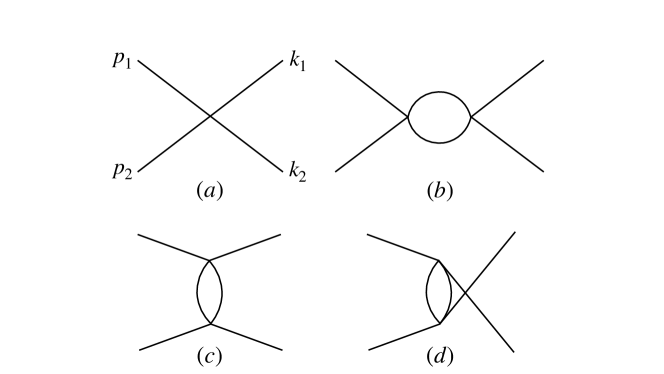
Figure 4: Diagrams contributing to the one-loop two-particle scattering amplitude, $\mathcal{M}_{2}$.

We now turn to the computation of the subtracted three-particle scattering amplitude at threshold, $\bar{\mathcal{T}}$. At leading order, the only diagram that contributes is like diagram (a) in Fig. 2 (including all nine combinations of incoming and outgoing particles). The tree-level result is:

$$\bar{\mathcal{T}}=\frac{9\lambda_{r}^{2}}{2m^{5}}=\frac{288\pi^{2}a_{0}^{2}}{m^{3}}.$$ (122)

4.1.1 Exponentially-suppressed corrections

The Eq. (85), which is used for the extraction of the scattering parameters from lattice simulations, contains only terms that vanish like powers of $L$. There are, however, exponentially-suppressed effects, which might be relevant. In order to take them into account, one can apply perturbation theory in the continuum and evaluate the corrections in the parameters that enter Eq. (85). In this manner, it is possible to explicitly include the leading exponential corrections into the fit.

We start from the single-particle mass, where the leading-order result of Ref. Gasser:1986vb will be used:

$$M_{\varphi}(L)=m+c_{M}\cdot\frac{K_{1}(mL)}{mL}\to m+c_{M}^{\prime}\frac{e^{-mL}}{(mL)^{3/2}}.$$ (123)

In this formula, $M_{\varphi}(L)$ denotes the finite-volume mass and $m$ the infinite-volume one. Further, $c_{M},c^{\prime}_{M}$ are constants whose exact value is not of interest at this stage, and $K_{\nu}(z)$ are the modified Bessel functions of second kind.

The leading exponentially-suppressed finite-volume correction to the scattering length can be calculated, following the strategy explained in Ref. Romero-Lopez:2018rcb . The result is given by:

$$a_{0}(L)=a_{0}\left(1-\frac{24ma_{0}}{\pi}K_{0}(mL)\right)\rightarrow a_{0}\left(1-\frac{24ma_{0}}{\sqrt{2\pi mL}}e^{-mL}\right).$$ (124)

4.2 Lattice simulation

For the numerical approach to complex scalar $\varphi^{4}$ theory, the discretization of space-time is required. This can be realized by introducing a finite hypercubic lattice of a volume $T\cdot L^{3}$. Here $T$ denotes the Euclidean time length of the lattice and $L$ is the spatial extension. Such a four-dimensional lattice can be described by means of discrete points $x^{\mu}$, separated by the lattice spacing $a$. In addition, periodic boundary conditions are assumed in all four directions. These are implemented by requiring

$$\varphi\left(x^{\mu}+Le^{\mu}\right)=\varphi\left(x^{\mu}\right)\,,\qquad \mbox{for}~{}\mu=1,2,3,$$

$$\varphi\left(x^{\mu}+Te^{\mu}\right)=\varphi\left(x^{\mu}\right)\,,\qquad \mbox{for}~{}\mu=4,$$ (125)

where $\varphi\left(x^{\mu}\right)\in\mathbb{C}$ is the complex scalar field and $e^{\mu}$ denotes a unit vector in the direction of axis $\mu$.

For the numerical simulation of field configurations, a discretization of the action is mandatory. This is realized by replacing the four-dimensional integral by a sum, as well as the partial derivatives by finite differences. Furthermore, introducing a hopping parameter $\kappa$, the fields are rescaled, according to

$$a\,\varphi\left(x^{\mu}\right)=\sqrt{\kappa}\,\varphi_{x}.$$ (126)

Similarly, the dimensionful mass $m$ is removed from the action by converting the terms, depending on absolute values of $\varphi_{x}$ to a binary quadratic form. For that purpose, we use the following relations:

$$\lambda_{0}=\frac{\lambda^{\prime}}{\kappa^{2}}\,,\quad\quad(am)^{2}=\frac{1-2\lambda^{\prime}-8\kappa}{\kappa}\,.$$ (127)

Taking this into account, the discretized expression for the action becomes:

$$S=\sum_{x^{\mu}}\left[\Bigg{(}-\kappa\sum_{\mu}\varphi_{x}^{*}\,\varphi_{x+\mu}+c.c.\Bigg{)}+\lambda^{\prime}\,\left(|\varphi_{x}|^{2}-1\right)^{2}+|\varphi_{x}|^{2}\right].$$ (128)

In the simulations, particle mass and coupling constant are set to $m^{2}=-4.9$ and $\lambda_{0}=10.0$, respectively. This leads to $\lambda^{\prime}=0.253308$, and $\kappa=0.159156$ in the discretized action, Eq. (128). This choice—identical to Ref. Romero-Lopez:2018rcb —has the advantage that it leads to a small renormalized coupling constant, which strongly suppresses excited states.

By means of Metropolis-Hastings simulations, ensembles are generated with constant $T=48$ and varying $L$ in the interval $L\in[6,24]$ (from now on, $L$ and $T$ will be given in lattice units). More extended lattices are not studied, because of the increased numerical cost. Likewise, smaller lattices with $L<6$ are not taken into account, as they are dominated by the boundaries, and marginally incorporate physical information. The different volumes and the corresponding number of produced configurations, as well as the volume-dependent number of Metropolis updates per thread are summarized in Tab. 1.

$L$	$n_{\text{conf}}$	ud$/$thr	$L$	$n_{\text{conf}}$	ud$/$thr
6	100,000	800	16	100,000	1880
7	100,000	800	17	100,000	2240
8	100,000	800	18	100,000	2800
9	100,000	800	19	100,000	3128
10	100,000	480	20	80,000	3800
11	100,000	800	21	70,000	4224
12	100,000	800	22	50,000	5000
13	100,000	1000	23	50,000	5544
14	100,000	1280	24	30,000	6400
15	100,000	1600

Table 1: Summary of simulations used in this work. $T=48$ is kept throughout. $n_{\text{conf}}$ labels the number of field configurations. The number of updates per thread, ud/thr, is provided as well. In order to decrease correlation, only every $1000^{\text{th}}$ configuration is saved.

4.2.1 Effective potential

The $\varphi^{4}$ theory has two distinct phases: the symmetric and the broken one. Before performing simulations, one wants to know, which phase is realized by a given choice of parameters. Our framework, used for the analysis of the multi-particle energy levels, can be used in the symmetric phase only, where the particle, described by the field $\varphi$, has a non-zero mass. In order to answer the above question, note that measuring the effective potential allows one to distinguish between the two phases: a monotonically growing potential is associated with the symmetric phase, whereas a “Mexican-hat” potential characterizes the broken phase.

The effective potential of the $\varphi^{4}$ can be computed by including a term in the action—with the coefficient $J$—that explicitly breaks the $U(1)$ global symmetry. The continuum Lagrangian in the presence of the symmetry-breaking term has the form:

$$\mathcal{L}=\partial_{\mu}\varphi^{*}\partial^{\mu}\varphi-m_{0}^{2}\varphi^{*}\varphi-\lambda_{0}(\varphi^{*}\varphi)^{2}-J|\varphi|.$$ (129)

This way, the effective (renormalized) potential

$$U(|\varphi|)=V(|\varphi|)+J|\varphi|=m^{2}\varphi^{*}\varphi+\lambda_{r}(\varphi^{*}\varphi)^{2}+J|\varphi|,$$ (130)

will have a minimum at

$$\frac{\text{d}U}{\text{d}|\varphi|}\Bigg{\rvert}_{\varphi=\langle\varphi\rangle}=0\longrightarrow J(\langle\varphi\rangle)=\frac{\text{d}V}{\text{d}|\varphi|}\Bigg{\rvert}_{\varphi=\langle\varphi\rangle}.$$ (131)

Now, by measuring $\langle\varphi\rangle$ as a function of $J$, we could infer the shape of the potential:

$${\frac{\text{d}V}{\text{d}|\varphi|}\Bigg{\rvert}_{\varphi=\langle\varphi\rangle}=a_{1}\,\langle\varphi\rangle+a_{2}\,\langle\varphi\rangle^{3}.}$$ (132)

We have performed the simulations on a $16^{4}$ lattice for different values of $J$, using the same $m_{0}$ and $\lambda_{0}$ as in the “main” simulations. The results are shown in Fig. 5.

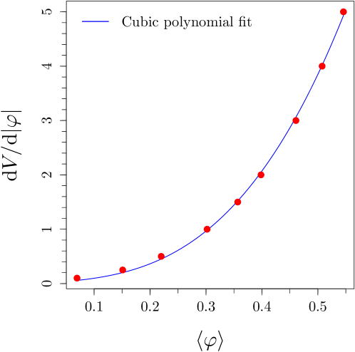
Figure 5: Derivative of the effective potential with respect to $|\varphi|$ as a function of $\langle\varphi\rangle$. The existing statistical errors on $\langle\varphi\rangle$ are too small to be visible. The blue curve corresponds to a cubic polynomial fit with Eq. (132).

The parameters obtained from the corresponding cubic polynomial fit read

$${a_{1}=0.70(13),~{}~{}~{}a_{2}=28.01(58).}$$ (133)

As can be seen, the shape of $\frac{\text{d}V}{\text{d}|\varphi|}$ is that of a positive monotonically growing function. This implies a monotonically growing effective potential, $V(\varphi)$. Therefore, we can confirm that the set of parameters, chosen for this work, corresponds to the symmetric phase of the $\varphi^{4}$ theory.

4.3 The operators and correlation functions

With the configurations from Tab. 1, the one- to five-particle correlators are computed. The errors are determined from the corresponding bootstrap samples (standard deviation). Then, particle energies are extracted by fitting the analytic form of the respective correlation function to the data. The $N$-particle correlation function can be written as:

$$C_{N}(t_{\text{in}},t_{\text{out}})=\Braket{\hat{\mathcal{O}}_{N\varphi}(t_{\text{out}})\,\hat{\mathcal{O}}_{N\varphi}^{\dagger}(t_{\text{in}})},$$ (134)

with

$$\hat{\mathcal{O}}_{N\varphi}=\left(\sum_{x}\varphi(x)\right)^{N}.$$ (135)

We restrict ourselves to $N=1,\dots,5$ henceforth. In Euclidean time, the temporal evolution of an operator generally reads

$$\hat{\mathcal{O}}(t)=e^{\hat{H}\,t}\,\hat{\mathcal{O}}(0)\,e^{-\hat{H}\,t}.$$ (136)

Considering this definition, with the source operator at the initial time $t_{\text{in}}=0$, and the sink operator at the final time $t_{\text{out}}=t$, Eq. (134) can be expressed as

$$C_{N}(t)=\frac{1}{Z}\,\text{Tr}\,\Bigg{[}e^{-\hat{H}\,(T-t)}\,\hat{\mathcal{O}}_{N\varphi}(0)\,e^{-\hat{H}\,t}\,\hat{\mathcal{O}}_{N\varphi}^{\dagger}(0)\Bigg{]}.$$ (137)

The trace occurring here is due to the periodic boundary conditions. It is the origin of the undesirable thermal pollutions of the correlation functions, that is, effects from particles propagating across the boundary backwards in time. In order to find the analytic form of the correlation function, Eq. (134) has to be expanded in an infinite sum of eigenstates, resulting in:

$$C_{N}(t) =\frac{1}{Z}\,\sum_{m,n}\left|\braket{n}{\hat{\mathcal{O}}_{N\varphi}}{m}\right|^{2}\,e^{-E_{n}\,(T-t)}\,e^{-E_{m}\,t}$$

$$=\frac{1}{Z}\,\sum_{m,n}\left|\braket{n}{\hat{\mathcal{O}}_{N\varphi}}{m}\right|^{2}\,e^{-(E_{m}+E_{n})\,\frac{T}{2}}\,\cosh\left((E_{m}-E_{n})\,(t-\tfrac{T}{2})\right).$$ (138)

Keeping only the leading terms, the explicit expressions of the one- to five-particle correlation function follows are:

$$C_{1}(t) =\big{|}A^{(1)}_{1\leftrightarrow 0}\big{|}^{2}\exp\left(-M_{\varphi}\tfrac{T}{2}\right)\,\cosh\left(M_{\varphi}(t-\tfrac{T}{2})\right)$$ (139)

$$C_{2}(t) =\big{|}A^{(2)}_{2\leftrightarrow 0}\big{|}^{2}\exp\left(-E_{2}\tfrac{T}{2}\right)\,\cosh\left(E_{2}(t-\tfrac{T}{2})\right)+\big{|}A^{(2)}_{1\leftrightarrow 1}\big{|}^{2}\exp\left(-M_{\varphi}T\right)$$ (140)

$$C_{3}(t) =\big{|}A^{(3)}_{3\leftrightarrow 0}\big{|}^{2}\exp\left(-E_{3}\tfrac{T}{2}\right)\,\cosh\left(E_{3}(t-\tfrac{T}{2})\right)$$

$$\quad+\big{|}A^{(3)}_{2\leftrightarrow 1}\big{|}^{2}\exp\left(-(E_{2}+M_{\varphi})\tfrac{T}{2}\right)\,\cosh\left((E_{2}-M_{\varphi})(t-\tfrac{T}{2})\right)$$ (141)

$$C_{4}(t) =\big{|}A^{(4)}_{4\leftrightarrow 0}\big{|}^{2}\exp\left(-E_{4}\tfrac{T}{2}\right)\,\cosh\left(E_{4}(t-\tfrac{T}{2})\right)$$

$$\quad+\big{|}A^{(4)}_{3\leftrightarrow 1}\big{|}^{2}\exp\left(-(E_{3}+M_{\varphi})\tfrac{T}{2}\right)\,\cosh\left((E_{3}-M_{\varphi})(t-\tfrac{T}{2})\right)$$

$$\quad+\big{|}A^{(4)}_{2\leftrightarrow 2}\big{|}^{2}\exp\left(-E_{2}T\right)$$ (142)

$$C_{5}(t) =\big{|}A^{(5)}_{5\leftrightarrow 0}\big{|}^{2}\exp\left(-E_{5}\tfrac{T}{2}\right)\,\cosh\left(E_{5}(t-\tfrac{T}{2})\right)$$

$$\quad+\big{|}A^{(5)}_{4\leftrightarrow 1}\big{|}^{2}\exp\left(-(E_{4}+M_{\varphi})\tfrac{T}{2}\right)\,\cosh\left((E_{4}-M_{\varphi})(t-\tfrac{T}{2})\right)$$

$$\quad+\big{|}A^{(5)}_{3\leftrightarrow 2}\big{|}^{2}\exp\left(-(E_{3}+E_{2})\tfrac{T}{2}\right)\,\cosh\left((E_{3}-E_{2})(t-\tfrac{T}{2})\right)$$ (143)

The first term in each of the previous equations includes the energy to be determined. Except for the single-particle correlator $C_{1}$ all functions exhibit thermal-pollution terms in addition to the “cosh” signal. In case of $C_{2}$, this term is time-independent, whereas the remaining ones contain time-dependent thermal effects. Although these vanish in the large $T$-limit, they will taken into account, as the analysis is restricted to the finite lattice volumes. For instance, time-independent terms can be removed by shifting the affected functions:

$$C_{N}^{\prime}(t+1/2)=C_{N}(t)-C_{N}(t+1).$$ (144)

This also allows to reduce the correlation between different time slices. The analytical form of the shifted correlators will be as in Eqs. (139)-(143), with $\cosh$ replaced by $\sinh$.

4.4 Fit strategies and parameter extraction

For the parameter extraction, the correlated fits are performed. When the correlation functions $C_{N}^{\prime}(t)$ with $N>2$ are examined, energy levels corresponding to lower numbers of particles, contribute to the time-dependent thermal pollution terms, cf. Eq. (139) to (143). Those terms will be taken into account in the fit. In order to increase the fit sensitivity to the $N$-particle energy $E_{N}$, lower lying energy levels, already determined in previous fits, may be used as priors for constraining the fit. This procedure is shown in the following scheme (145):

$$C_{2}^{\prime}(t)\xrightarrow{E_{2}-M_{\varphi}}C_{3}^{\prime}(t)\xrightarrow{E_{3}-M_{\varphi}}C_{4}^{\prime}(t)\xrightarrow{E_{4}-M_{\varphi},E_{3}-E_{2}}C_{5}^{\prime}(t)$$ (145)

Hence, the best fit parameters obtained previously—shown on top of the arrows—enter the current fit as priors. The $\chi^{2}$-function has to be modified accordingly:

$$\chi^{2}\longrightarrow\chi^{2}+\sum_{i=1}^{k-1}\left(\frac{P_{p_{i}}-p_{i}}{\Delta p_{i}}\right)^{2}.$$ (146)

Here, $P_{p_{i}}$ denotes the prior applied to constrain the $i^{\text{th}}$ parameter $p_{i}$ and $\Delta p_{i}$ the corresponding standard error. Finally, the energy shifts with respect to the free energies are computed as:

$$\Delta E_{N}(L)=E_{N}(L)-N\cdot M_{\varphi}(L)~{}~{}~{}\text{with}~{}~{}~{}M_{\varphi}(L)\equiv E_{1}(L),$$ (147)

including the corresponding bootstrap samples. Note that the volume-dependent mass is used for the computation of the shift, as it has been shown to cancel the leading exponentially-suppressed effects Romero-Lopez:2018rcb .

The first quantity to be studied is the single-particle mass $M_{\varphi}(L)$ and its volume-dependence. This is relevant because the mass enters in the threshold expansion in Eq. (85). We will use the infinite-volume mass, $m$, obtained by fitting Eq. (123) to the $M_{\varphi}(L)$ data. In practice, using $m$ or $M_{\varphi}(L)$ in Eq. (85) induces only higher-order exponentially-suppressed effects.

Once the infinite-volume mass is determined, different strategies are carried out to fit the energy shifts:

1. Fixed-$N$ fits. Here the energy shifts of $N$ particles are fitted separately. For $N>2$, we also employ $a_{0}$ and $r_{0}$ as priors. For this, the $a_{0}$ and $r_{0}$, extracted from the two-body sector, are used as input for the analysis of the three- to five-body sector. Priors in $r_{0}$ are crucial to disentangle $r_{0}$ and $\bar{\mathcal{T}}$, as the two parameters enter at the same order. This also increases the fit sensitivity for the threshold amplitude $\bar{\mathcal{T}}$. According to the prescription in Eq.(146), the modification of the $\chi^{2}$-function is given by

   $$\chi^{2}\rightarrow\chi^{2}+\left(\frac{P_{a_{0}}-a_{0}}{\Delta a_{0}}\right)^{2}+\left(\frac{P_{r_{0}}-r_{0}}{\Delta r_{0}}\right)^{2}.$$ (148)

2. Unconstrained global fits. This fit includes all data with $N=2-5$. It is based on the determination of the values of $\{a_{0},r_{0},\bar{\mathcal{T}}\}$ that minimize the sum of all contributing $\chi^{2}$-functions, i.e.,

   $$\chi^{2}_{\text{global}}(\tilde{p})=\sum_{N=2}^{5}\,\sum_{i\in D}\frac{\left[\Delta E_{N,\text{d}}(L_{i})-\Delta E_{N}(L_{i},\tilde{p})\right]^{2}}{\left[\Delta(\Delta E_{N,\text{d}}(L_{i}))\right]^{2}}.$$ (149)

   Here, $\tilde{p}$ denotes a vector containing all fit parameters. Furthermore, $d$ labels the data, $L_{i}$ denote the sizes of different boxes used in the calculations, and $D$ represents a complete set of ensembles.

3. Prior-constrained global fits. In this case, the data with $N=3-5$ is considered, and we include priors in $a_{0},r_{0}$ from the $\Delta E_{2}$-fits.

Finally, it is very important to check the convergence of the $1/L$ expansion of the energy shifts. For this purpose, we study the phase shift, extracted from the Lüscher formalism Luscher:1991n1 , and compare it to the scattering parameters, obtained from the various fits to Eq. (85). According to Luscher:1991n1 , the $S$-wave phase shift is determined by

$$\cot(\delta)=\frac{Z_{00}(1,q^{2})}{\pi^{3/2}\,q}\qquad\text{with}\qquad q=\frac{L\,k}{2\pi}$$ (150)

and the Lüscher zeta function $Z_{00}$. The momentum $k$ can be calculated as

$$E_{2}=2\sqrt{k^{2}+M_{\varphi}(L)^{2}}.$$ (151)

Furthermore, the effective-range expansion at order $k^{6}$ reads

$$k\cot(\delta)=-\frac{1}{a_{0}}+\frac{r_{0}k^{2}}{2}-Pr_{0}^{3}k^{4}+\mathcal{O}(k^{6}),$$ (152)

where $P$ denotes the $S$-wave shape parameter. Starting from this expansion, four different models are set up, as summarized in Tab. 2. They are fitted to the phase-shift data, calculated from Eq. (150) using bootstrap samples. This allows to extract both $a_{0}$ and $r_{0}$ independently from the $N$-particle ground-state fits. In case of model (IIa) and (IIb), the $S$-wave shape parameter $P$ is obtained in addition. The “a” and “b” models should be equivalent, and they allow us to explore the systematics of different fitting techniques.

(Ia)	$\delta(k)=\arctan\left[\left(-\frac{1}{a_{0}k}+\frac{r_{0}k}{2}\right)^{-1}\right]$
(Ib)	$k\cot\left[\delta(k)\right]=-\frac{1}{a_{0}}+\frac{r_{0}k^{2}}{2}$
(IIa)	$\delta(k)=\arctan\left[\left(-\frac{1}{a_{0}k}+\frac{r_{0}k}{2}-Pr_{0}^{3}k^{3}\right)^{-1}\right]$
(IIb)	$k\,\cot\left[\delta(k)\right]=-\frac{1}{a_{0}}+\frac{r_{0}k^{2}}{2}-Pr_{0}^{3}k^{4}$

Table 2: $S$-wave phase-shift fit models.

4.5 Results

In this section, the numerical results are presented. The material is organized as follows. First, the volume-dependence of the single-particle mass is analyzed. Then, the energy shifts are investigated at order $L^{-5}$. After that, the results, obtained from different types of fits at $O(L^{-6})$—described in Section 4.4—are presented. The effects of relativistic and exponentially-suppressed corrections are studied separately. Finally, the results, obtained from the lattice simulations, are compared to the corresponding perturbative predictions.

4.5.1 Volume dependence of the mass

The results from the fits of the mass to Eq. (123) for different ranges of $L$ are summarized in Tab. 3. The best result for the infinite-volume mass is obtained from the range $[8,24]$:

$$m=0.20368(17),~{}~{}~{}\chi^{2}/\text{ndof}=13.13/15,~{}~{}~{}p\text{-value}=0.59$$ (153)

The corresponding curve is shown in Fig. 6, suggesting that a rough approximation $M_{\varphi}(L)\approx m$ is valid for $L\geq 20$, or equivalently, $M_{\varphi}(L)L\geq 4$. In the forthcoming analysis, the numerical result in Eq. (153) will be used, when fitting to Eq. (85).

fit interval	$M_{\infty}$	$c_{M}$	$\chi^{2}/\text{ndof}$	$p$-value
$[6,24]$	0.20441(15)	0.19079(84)	$134.17/17=7.89$	0.00
$[7,24]$	0.20393(16)	0.2007(13)	$42.87/16=2.68$	2.93e-04
$[8,24]$	0.20368(17)	0.2107(22)	$13.13/15=0.88$	0.59
$[9,24]$	0.20352(18)	0.2201(48)	$8.20/14=0.59$	0.88
$[10,24]$	0.20345(19)	0.2251(61)	$6.52/13=0.50$	0.93

Table 3: Results, obtained from the single-particle mass fits.

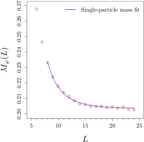
Figure 6: Volume dependence of the single-particle mass. The lattices with temporal extension $T=48$ are considered. The blue curve corresponds to the fit in the range [8,24] for $L$.

4.5.2 $N$-particle ground state to order $L^{-5}$

We start by studying the energy shifts at order $L^{-5}$. At this order, all energies are solely described by the scattering length. First, the ratios of energy shifts are explored. Because of the binomial coefficients, occurring in the $N$-particle threshold expansion, Eq. (85), these ratios behave as:

$$\frac{\Delta E_{N}}{\Delta E_{2}}=\binom{N}{2}+\mathcal{O}\left(L^{-5}\right).$$ (154)

The results are shown in Fig. 7, where it can be seen that the values are in a right ballpark. The accuracy of the energy shift ratios, however, does not suffice for reliable parameter extraction. For this reason, Fig. 7 should only be considered as a rough quality test of the simulation.

fit	EC	$a_{0}$	$\chi^{2}/\text{ndof}$	$p$-value
$\Delta E_{2}$	$\times$	0.421(18)	$7.42/10=0.74$	0.69
	$\checkmark$	0.428(18)	$7.17/10=0.72$	0.71
$\Delta E_{3}$	$\times$	0.441(16)	$4.66/10=0.47$	0.91
	$\checkmark$	0.449(16)	$4.29/10=0.43$	0.93
$\Delta E_{4}$	$\times$	0.425(15)	$8.18/10=0.82$	0.61
	$\checkmark$	0.432(15)	$7.90/10=0.79$	0.64
$\Delta E_{5}$	$\times$	0.410(14)	$8.77/10=0.88$	0.55
	$\checkmark$	0.418(15)	$8.46/10=0.85$	0.58

Table 4: Comparison of the results obtained from the energy shift fits to order $L^{-5}$ in the interval $[14,24]$. We provide the results with as well as without EC

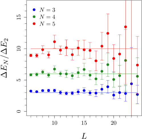
Figure 7: Energy shift ratios in dependency of the lattice parameter $L$. For orientation the colored straight lines mark the ratio values $3,6,10$.

Next, we perform fits to the threshold expansion up to the same order. To this end, we truncate Eq. (85) at $O(L^{-5})$, and include only the data at larger values of $L$, for which this approximation should be valid. We separate fits for $N=2,3,4$ and $5$, and obtain $a_{0}$. The best fit range is determined by varying the lower bound of the fit interval, while the upper one is kept fixed at $L=24$. The best choice turns out to be $[14,24]$, for which the results are summarized in Tab. 4. We also perform a fit, including the exponentially-suppressed corrections (EC) of Eq. (124). As expected, the results with and without EC match reliably. This means that, for the values of $L$, considered here, the EC are weak, and vanish within the range of statistical errors. Moreover, the fits for different values of $N$ agree nicely within the uncertainty.

4.5.3 Fixed-$N$ fits to order $L^{-6}$

In order to extract information on the three-body interactions—parameterized by the quantity $\bar{\mathcal{T}}$—the fits at order $O(L^{-6})$ should be performed. We start with the fixed-$N$ fits as described in Section 4.4. We first fit $\Delta E_{2}$, and use $a_{0},r_{0}$ as priors for $N>2$. The selected results come from the interval $[9,24]$. We shall try various fit models to explore the effects of EC and relativistic corrections (RC). The latter are the $O(L^{-6})$ terms in Eq. (85) that vanish, when $m\to\infty$. All results are displayed Tab. 5.

fit	EC	RC	$a_{0}$	$r_{0}$	$\bar{\mathcal{T}}$	$\chi^{2}/\text{ndof}$	$p$-value
$\Delta E_{2}$	$\times$	$\times$	0.430(16)	$-319(17)$	$-$	$12.31/14$	0.58
	$\times$	$\checkmark$	0.430(16)	$-291(17)$	$-$	$12.31/14$	0.58
	$\checkmark$	$\times$	0.432(16)	$-$256(17)	$-$	$11.69/14$	0.63
	$\checkmark$	$\checkmark$	0.432(16)	$-$228(18)	$-$	$11.69/14$	0.63
$\Delta E_{3}$	$\times$	$\times$	0.426(14)	$-314(16)$	$-354647(40323)$	$20.08/15$	0.17
	$\times$	$\checkmark$	0.426(14)	$-286(17)$	$-262938(35766)$	$20.08/15$	0.17
	$\checkmark$	$\times$	0.428(14)	$-251(16)$	$-289575(36963)$	$19.18/15$	0.21
	$\checkmark$	$\checkmark$	0.428(14)	$-222(17)$	$-196974(32676)$	$19.18/15$	0.21
$\Delta E_{4}$	$\times$	$\times$	0.432(13)	$-315(16)$	$-348072(38974)$	$18.12/15$	0.26
	$\times$	$\checkmark$	0.432(13)	$-287(16)$	$-253866(34474)$	$18.12/15$	0.26
	$\checkmark$	$\times$	0.434(13)	$-252(16)$	$-280922(35690)$	$17.63/15$	0.28
	$\checkmark$	$\checkmark$	0.434(13)	$-224(17)$	$-185831(31390)$	$17.63/15$	0.28
$\Delta E_{5}$	$\times$	$\times$	0.431(13)	$-316(17)$	$-341000(38374)$	$16.75/15$	0.33
	$\times$	$\checkmark$	0.431(13)	$-288(17)$	$-247376(33891)$	$16.75/15$	0.33
	$\checkmark$	$\times$	0.433(13)	$-253(17)$	$-274134(35092)$	$16.41/15$	0.36
	$\checkmark$	$\checkmark$	0.433(13)	$-225(17)$	$-179652(30784)$	$16.41/15$	0.36

Table 5: The results, obtained from the fixed-$N$ energy shift fits at order $L^{-6}$ in the interval $[9,24]$ with and without EC and RC. The results for $a_{0}$ and $r_{0}$ obtained from the $\Delta E_{2}$-fit serve as priors in the remaining fits.

The fit results for $a_{0}$ are in agreement with the findings from the fits at order $L^{-5}$, cf. Tab. 4. As can be seen, the fit quality—represented by $\chi^{2}/\text{ndof}$ and $p$-value—is not affected by the RC. Yet, it slightly improves when EC is included. On the other hand, both RC and EC modify significantly the best fit parameters. Since the change is comparable to—or even larger than—the statistical error, It is important to include these effects in the fit.

4.5.4 Global $N$-particle ground-state fits

In order to increase the fit sensitivity for $\bar{\mathcal{T}}$, it is appropriate to try another strategy, namely, a combined fit of Eq. (85) to the energy shifts $\Delta E_{N=2,3,4,5}$. Furthermore, global fits to the $\Delta E_{N=3,4,5}$ data with prior-constrained scattering length (or both $a_{0}$ and $r_{0}$), determined from the $\Delta E_{2}$-fit to order $L^{-6}$, are conducted. Again, the lower fit interval limit is varied, while the upper one stays fixed at $L=24$. The best results are obtained from the fit interval $[10,24]$. They are summarized in Tab. 6.

priors	EC	RC	$a_{0}$	$r_{0}$	$\bar{\mathcal{T}}$	$\chi^{2}/\text{ndof}$	$p$-value
$-$	$\times$	$\times$	0.438(15)	$-320(21)$	$-362327(52137)$	$52.83/57$	0.63
$-$	$\times$	$\checkmark$	0.438(15)	$-292(21)$	$-265422(46637)$	$52.83/57$	0.63
$-$	$\checkmark$	$\times$	0.439(15)	$-255(22)$	$-286929(47814)$	$52.29/57$	0.65
$-$	$\checkmark$	$\checkmark$	0.439(15)	$-227(22)$	$-189799(42507)$	$52.29/57$	0.65
$a_{0}$	$\checkmark$	$\checkmark$	0.443(15)	$-207(25)$	$-165483(45346)$	$37.19/43$	0.72
$a_{0}$, $r_{0}$	$\checkmark$	$\checkmark$	0.450(12)	$-234(18)$	$-216760(31039)$	$42.05/44$	0.56

Table 6: Comparison of the results, obtained from the global energy shift fits to order $L^{-6}$ in the interval $[10,24]$ with and without using priors, EC and RC. The four results above the horizontal line correspond to the fits without priors. The last two results are fits, for which the parameter(s) $a_{0}$ ($a_{0}$ and $r_{0}$) obtained from the corresponding $\Delta E_{2}$-fit within the interval $[10,24]$ serve(s) as prior(s).

For illustrative purposes, a global fit with EC as well as RC without any prior knowledge is shown in Fig. 8.

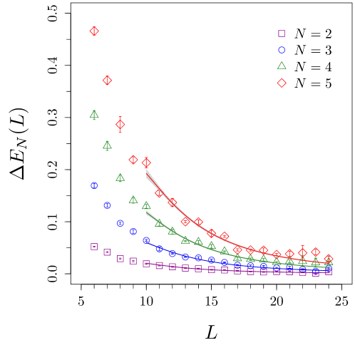
Figure 8: Global fit without priors in the interval $[10,24]$ for $L$. Both EC and RC are included.

The results without priors are highly consistent with those from the previous fixed-$N$ fits to order $L^{-6}$, cf. Tab. 5. Similarly to the fixed-$N$ fits, EC slightly improve the fit quality, and both RC and EC affect the best fit parameters beyond the size of the statistical error. If only $a_{0}$ is used as prior, the fit is consistent but errors remain comparable. Yet, the inclusion of priors in $a_{0}$ and $r_{0}$ reduces notably the statistical errors, while changing the best fit parameters only by order the statistical error. Remarkably, in this last fit we observe that $\bar{\mathcal{T}}\neq 0$ with $7\sigma$ considering only the statistical error.

4.5.5 Phase-shift fits

In order to check the convergence of the $1/L$ expansion, we will compare the previous fit results to the ones from the full Lüscher formalism—see Eq. (150). All fit models, used in the phase-shift analysis, are listed in Tab. 2. In general, the best results are obtained from the fits to the complete set of data points. This is particularly important for the fit models that include the shape parameter, $P$. The results are summarized in Tab. 7.

As it can be seen, the results from fits, which are using model (Ia) and (Ib), are in good agreement with the previous findings, which are obtained from the perturbative expansion of the the $N$-particle ground-state energies, cf. with Tabs. 4, 5 and 6. In contrast, the results from the fits with (IIa) and (IIb) do not seem to match those from the energy shift fits. A potential explanation could be provided by exponentially-suppressed effects that have been seen to be relevant before—see e.g. Tab. 6—and are not considered in the phase-shift data points. It is important to note that we must include points with large $k^{2}$ to fit the parameter $P$ reliably. However, these points originate from simulations with $L<8$, and exponentially-suppressed effects can be very significant. To check this, in Fig. 9 we plot the results from the fits (Ib) and (IIb) along with the predictions, based on the results for $a_{0}$ and $r_{0}$, obtained from the global energy shift fits in Tab. 6. If EC are not included in the expansion of the energy levels, the resulting line describes the red data points very well. From this, one can conclude two things: (i) the convergence of the $1/L$ is not of a concern here, and (ii) EC produce a visible impact. A side observation is that RC are also noticeable in the phase-shift curve.

fit model	$a_{0}$	$r_{0}$	$P$	$\chi^{2}/\text{ndof}$	$p$-value
(Ia)	0.407(17)	$-274(23)$	$-$	$14.63/17=0.86$	0.62
(Ib)	0.419(16)	$-285(21)$	$-$	$28.20/17=1.66$	0.04
(IIa)	0.483(36)	$-534(93)$	$0.000049(19)$	$10.13/16=0.63$	0.86
(IIb)	0.474(33)	$-494(89)$	0.000052(35)	$19.96/16=1.25$	0.22

Table 7: Results from the different $S$-wave phase-shift fits to the complete set of data points.

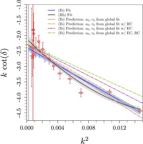
Figure 9: Comparison of the phase-shift fit, which is using the model (Ib) as well as (IIb), with the predictions from the global fit without priors. All predictions, displayed here, are based on the model (Ib) and involve the scattering parameters, obtained from the global fits shown in Tab. 6. Both fit curves are plotted with error bands. The corresponding fit results are listed in Tab. 7.

4.5.6 $N$-particle ground-state fits with perturbative constraints

As explained in Section 4.1, in the $\varphi^{4}$ theory, the different scattering parameters are determined by a single coupling constant. A rough estimate for $r_{0}$ and $\bar{\mathcal{T}}$ in perturbation theory, which can be obtained with $m\approx 0.2$ and $a_{0}\approx 0.4$, are:

$$r_{0,\text{pt}}\approx-50\qquad\text{and}\qquad\bar{\mathcal{T}}_{\text{pt}}\approx 57000.$$ (155)

It is however surprising to see that the perturbative results are $\sim 9\sigma$ away from the best global fit in Tab. 6. As an attempt to understand the reason for this discrepancy, one could enforce the constraints of Eqs. (121) and (122) in the threshold expansion [Eq. (85)]. This way, the fits would have a reduced number of free parameters. In that context, different ansätze for a modification of Eq. (85) are studied. We can either simultaneously constrain both $r_{0}$ and $\bar{\mathcal{T}}$ by their one-loop values, or just one of them. The best results, stemming from global fits with $L\in[12,24]$ are shown in Tab. 8. There we also show the perturbative expectations for $r_{0}$ and $\bar{\mathcal{T}}$, labeled $r_{0,\text{pt}}$ and $\bar{\mathcal{T}}_{\text{pt}}$.

fit[PC; PR]	$a_{0}$	$r_{0}$	$\bar{\mathcal{T}}$	$p$-val.	$r_{0,\text{pt}}$	$\bar{\mathcal{T}}_{\text{pt}}$
$\text{global}[r_{0};\times]$	0.412(11)	$-$	42559(12695)	0.46	$-$48(2)	57101(3052)
$\text{global}[r_{0};\checkmark]$	0.414(11)	$-$	40462(13274)	0.34	$-$48(2)	57656(3067)
$\text{global}[\bar{\mathcal{T}};\times]$	0.412(12)	$-37(10)$	$-$	0.43	$-48(2)$	57101(3329)
$\text{global}[\bar{\mathcal{T}};\checkmark]$	0.415(13)	$-40(12)$	$-$	0.24	$-48(2)$	57935(3633)
$\text{global}[r_{0},\bar{\mathcal{T}};\times]$	0.423(11)	$-$	$-$	0.14	$-47(1)$	60190(3134)
$\text{global}[\times;\times]$	0.491(24)	$-334(48)$	$-443857(134298)$	0.89	$-39(2)$	81074(7925)

Table 8: Results from the different energy shift fits with perturbative constraints (PC). Both fixed-$N$ fits ($\Delta E_{N},N=2,3,4,5$) and global fits to order $L^{-6}$ are listed, without as well as with $a_{0}$ priors (PR), obtained from the respective $\Delta E_{2}[r_{0};\times]$-fit. In case of combined fits without $a_{0}$ priors, $\Delta E_{2}$ contributes, in contrast to global fits with priors. All fits are performed in the interval $[12,24]$ for $L$, and they include EC as well as RC. The perturbative predictions $r_{0,\text{pt}}$ and $\bar{\mathcal{T}}_{\text{pt}}$ are calculated from Eqs. (121) and (122), using the corresponding values of $a_{0}$.

If only $r_{0}$ is constrained, the best fit result for $\bar{\mathcal{T}}$ is about $1.5\sigma$ away from the perturbative prediction. Alternatively, if $\bar{\mathcal{T}}$ is constrained, $r_{0}$ is also in $\sim 1\sigma$ agreement with perturbation theory. Constraining both also produces a similar result. All these fits are seemingly reasonable. Yet, if no constraints are applied, the fit quality—see the $p$-value—moderately improves, while the best fit results for $\bar{\mathcal{T}}$ and $r_{0}$ strongly differ from the perturbative predictions. This remains an open question, that will be addressed in the next section.

4.5.7 Final assessment of results

We have extracted the two- and three-particle scattering parameters using the $N$-particle ground state of simulations in complex $\varphi^{4}$ theory in the symmetric phase. Reviewing the results discussed in the previous sections, one can see that the different fit strategies seem to agree with each other. More specifically, it can be stated that $a_{0}$ is consistent, independently of the applied fit method. Nevertheless, we have noticed a concerning tension of $\sim 9\sigma$ between our unconstrained fit results and the predictions of the perturbation theory. This deviation affects two parameters, $r_{0}$ and $\bar{\mathcal{T}}$, whose contribution is very subleading—they appear first at $O(L^{-6})$. To illustrate this discrepancy, a comparison between the phase shift and the perturbative prediction is shown in Fig. 10. In this plot, the perturbative prediction uses the value of $a_{0}$ from the fit to $\Delta E_{2}$ at order $L^{-5}$ (with and without EC), and $r_{0}$ from Eq. (155), corresponding to the same $a_{0}$. At this stage, it is obvious that the strong deviations cannot emerge from the statistical fluctuations.

In Section 4.5.5, we have also checked that the $1/L$ expansion seems to be converging properly. In addition, we have explicitly accounted for the leading exponentially-suppressed effects. Besides this, we note that the impact of EC in the perturbative prediction is minimal—see Fig. 10. Even though subleading EC effects could contribute, it seems unlikely that they are sizable.

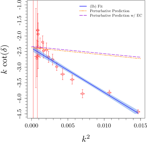
Figure 10: Comparison of the phase-shift fit using model (Ib) with perturbative predictions. The latter are computed by the scattering length extracted from the $\Delta E_{2}$ energy shift fits to order $L^{-5}$.

At this point, there remain very few explanations for this discrepancy. One possibility could be discretization effects. In order to study this, one could perform a Symanzik analysis Symanzik:1979ph . The idea is to write down the effective Lagrangian of the theory, including higher-dimensional operators that account for the cutoff effects. The contribution to the Lagrangian in the Euclidean space from the dimension-6 operators is

$$\Delta\mathcal{L}_{6}=a^{2}c_{1}\left(\varphi^{*}\partial_{\mu}\varphi\,\varphi^{*}\partial_{\mu}\varphi+\text{ h.c.}\right)+a^{2}c_{2}\partial_{\mu}\varphi^{*}\partial_{\mu}\varphi\varphi^{*}\varphi+a^{2}c_{3}\left(\varphi^{*}\varphi\right)^{3}.$$ (156)

As can be seen, both $c_{1}$ and $c_{2}$ contribute at tree-level to the two-particle scattering amplitude, and particularly to $a_{0}$ and $r_{0}$. Moreover, all three coefficients $c_{1},c_{2},c_{3}$ contribute at the three level to $\bar{\mathcal{T}}$. The crucial point is that the discretization effects are of the order $(aM)^{2}\sim 0.04$. However, a measure of the strength of the interactions, $Ma_{0}\sim 0.08$, is of the same order. Thus, it is plausible that cutoff effects could be significant, and so the continuum perturbation theory would not be an appropriate description of the lattice $\varphi^{4}$ theory with our set of parameters.

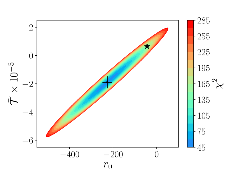
Figure 11: $\chi^{2}$ heat map that corresponds to the global fit at order $L^{-6}$ without priors, taking both EC and RC into account. The fit interval is $[10,24]$, and $a_{0}$ is fixed to 0.439. The black data point with error bars marks the corresponding fit results for $r_{0}$ and $\bar{\mathcal{T}}$, cf. Tab. 6. The black star marks the perturbative prediction.

To gain further insight into the above discrepancy and the fit systematics, we study the shape of the $\chi^{2}$ function for the previously discussed energy shift fits to order $L^{-6}$. For this, we use heat map plots to localize emerging minima and identify potential quasi-flat directions. Furthermore, the best fit parameters can then be easily compared with perturbative predictions. For a two-dimensional visualization in the $r_{0}$, $\bar{\mathcal{T}}$ plane, $a_{0}$ is fixed to the best fit result. We show the heat map plot for a global fit with EC and RC in Fig. 11. There, one can see that the $\chi^{2}$ function grows much slower in one particular direction in the $r_{0}$, $\bar{\mathcal{T}}$ plane. This happens, because in Eq. (85), the dependence on $r_{0}$ and $\bar{\mathcal{T}}$ can only be disentangled by considering different values of $N$. This feature increases the difficulty of measuring $\bar{\mathcal{T}}$ with statistical significance. In the Appendices B and C we discuss further heat map plots.

Since the inconsistency between perturbation theory and the unconstrained fit could not be resolved even after many different tests, we conclude that the perturbative results do not describe the lattice $\varphi^{4}$ theory properly. Beyond that, Fig. 11 displays the challenges that arise, when extracting low energy scattering parameters on the lattice. Namely, is clearly demonstrates the difficulty of extracting subleading effects and separating two- and three-body effects in the spectrum.

5 Conclusions and outlook

In the present paper, we discuss the derivation of the formula for the finite-volume energy shift of $N$ identical relativistic bosons in detail, up to and including $O(L^{-6})$. Moreover, in case of two- and three-particle systems, the derivation is extended to the first excited state, which is contained in the irreducible representations $A_{1}^{+}$ and $E^{+}$ of the cubic group. The derivation is performed in the framework of a non-relativistic effective theory, and relativistic effects are included perturbatively. Moreover, if needed, using the same effective Lagrangian, the derivation can be straightforwardly extended to higher excited states, and to excited states of systems containing more particles. This paper contains the necessary prescription in order to carry out such calculations.

We have also calculated finite-volume energy levels in the sectors with one, two, three, four and five identical bosons in the symmetric phase of the complex $\varphi^{4}$ theory on the lattice for many different values of the box size $L$. The wealth of the available lattice data enables us to carry out fits using different fit strategies, aiming at finding an optimal way to extract infinite-volume observables from the measured spectrum.

The main goal of lattice calculations is to establish few parameters (effective couplings), which describe the interactions in multiparticle systems. Only three parameters contribute at order in $1/L$ we are working. These are: the two-body scattering length $a_{0}$ and the effective range $r_{0}$, as well as the non-derivative three-body coupling that can be traded for the threshold amplitude $\bar{\mathcal{T}}$. The latter is of our primary concern. It turns out that $a_{0}$ can be reliably determined in all fits, whereas $r_{0}$ and $\bar{\mathcal{T}}$ are correlated in the fixed-$N$ fits. Only performing a global fit, involving sectors with different $N$, enables one to fix these parameters at a reasonable precision. The three-particle amplitude, $\bar{\mathcal{T}}$, turns out to be different from zero at $7\sigma$, taking into account only statistical error. Still, the $\chi^{2}$ heat map in the parameters $r_{0},\bar{\mathcal{T}}$ represents a rather elongated ellipse that indicates a strong correlation. It is important to stress also that this property stems merely from the way these two parameters enter the expression of the ground-state energy shift of $N$-particles at order $L^{-6}$. In this sense, it does not depend on the dynamics and will show up in QCD as well.

From this point of view, the study of the excited states becomes particularly interesting. As it is clear from the explicit expressions that are contained in the present paper, in excited states the relativistic and the effective-range corrections contribute already at order $L^{-5}$, whereas the contribution from $\bar{\mathcal{T}}$ emerges again first at order $L^{-6}$. Moreover, the contribution from $\bar{\mathcal{T}}$ is present in certain irreducible representations and is absent in others. All this gives hope that the study of the excited states might help one to break the spell of large correlations between extracted parameters. It would be certainly interesting to study this issue in the future.

The study of the role of relativistic effects, as well as leading-order exponentially-suppressed polarization effects was one of the main aims of the present work. We have shown that at the values of $L$ considered, both effects are substantial in the sense that including them in the fit leads to the changes in some observables beyond one standard deviation. This circumstance must be kept in mind when analyzing data from lattice QCD.

We have explicitly observed that finite lattice spacing effects might have a substantial impact on the values of the extracted parameters. In our example, the continuum theory badly fails to predict the values of $r_{0}$ and $\bar{\mathcal{T}}$, which are determined on the lattice. This fact should be also remembered when extracting the corresponding observables in lattice QCD that contribute at the subleading order(s) in the $1/L$ expansion.

Appendix A The finite parts of the two-loop diagrams

The finite parts of the two-loop diagrams in Eq. (52) in the chosen configuration of the external momenta are given by the following integrals over the Feynman parameters:

$$\delta^{(d)} = \frac{1}{2}\,\ln 3-\ln 2+\frac{1}{9}\,\sum_{(ijk)}\sum_{(lmn)}\int_{0}^{1}dx\int_{0}^{1}\frac{dy}{2\sqrt{y}}\,\biggl{(}\ln g-\frac{1-y}{g}\,\frac{dg}{dy}\biggr{)}\simeq-1.08964,\,$$

$$g = \frac{1}{4}\,(1-y)^{2}+\frac{1}{2}\,(1-y)+2y+\frac{1}{2}\,(1-y)^{2}x(1-x)(a_{kn}-1)\,,$$ (157)

and

$$\delta^{(e)} = -\frac{1}{9}\,\sum_{(ijk)}\sum_{(lmn)}\int_{0}^{1}dx\int_{0}^{1}\frac{ydy}{h^{3/2}}\,\biggl{(}-\ln G+\frac{3}{2}\,\ln h\biggr{)}\,\simeq 3.92587,$$

$$h = (1-y)-\frac{1}{4}\,(1-y)^{2}+x(1-x)y^{2}\,,$$

$$G = -\frac{3}{8}\,(1-y)(y-3)-y^{2}x(1-x)\biggl{(}-1+\frac{y}{4}+\frac{1}{4}\,(1-y)a_{kn}\biggr{)}\,.$$ (158)

In these equations, $a_{kn}={\bf p}_{k}^{\prime}{\bf p}_{n}/\lambda^{2}$. According to Eq. (32),

$$a_{kn}=\frac{1}{2}-\frac{3}{2}\delta_{kn}.$$ (159)

Appendix B $\chi^{2}$ heat map for the $\Delta E_{2}$-fit to order $L^{-6}$

Fig. 12 depicts the $\chi^{2}$ heat map, corresponding to the $\Delta E_{2}$-fit to order $L^{-6}$ in the interval $[9,24]$, including EC as well as RC. Here, we follow the visualization convention of Fig. 11. As expected, a distinct minimum that can be observed, is in agreement with the parameters obtained from the corresponding fit (black data point with error bars, cf. Tab. 5). The black star marks the corresponding perturbative prediction. Similarly to other fits in this work, the perturbative prediction is far from the best fit results.

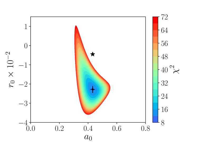
Figure 12: $\chi^{2}$ heat map that corresponds to the $\Delta E_{2}$-fit to order $L^{-6}$ taking both EC and RC into account. The fit interval is $[9,24]$, and $a_{0}$ is fixed to 0.432. The black data point with error bars marks the corresponding fit result for $r_{0}$, cf. Tab. 5. The black star corresponds to the perturbative prediction.

Appendix C $\chi^{2}$ heat map for the $\Delta E_{N}$-fits to $L^{-6}$

In this appendix, we show some additional heat map plots in order to explore the impact of priors in our fits – see Fig. 13. As already explained, $r_{0}$ and $\bar{\mathcal{T}}$ cannot be disentangled in a fixed-$N$ fit with $N>2$, because they enter at the same order in the threshold expansion. This is seen very well in Figs. 13, 13 and 13, as a flat direction with constant $\chi^{2}$. If priors from the $\Delta E_{2}$-fit are used for $r_{0}$, the flat direction disappears and $r_{0}$ and $\bar{\mathcal{T}}$ can be obtained – see Figs. 13, 13, and 13.

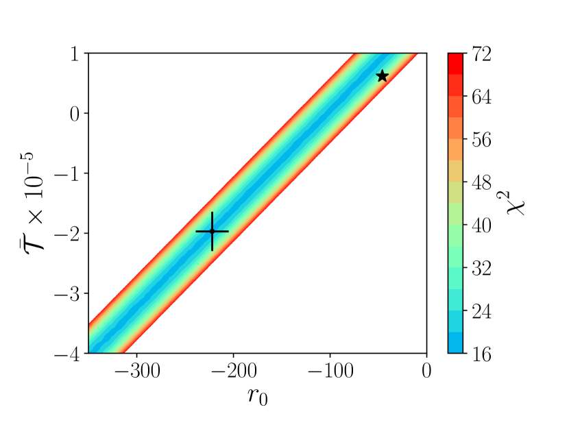
(a) Heat map for $\Delta E_{3}$-fit to order $L^{-6}$
without priors; $a_{0}$ is fixed to 0.428.

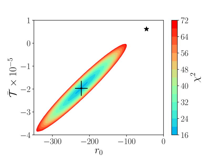
(b) Heat map for $\Delta E_{3}$-fit to order $L^{-6}$
with priors, cf. Tab. 5; $a_{0}$ is fixed to 0.428.

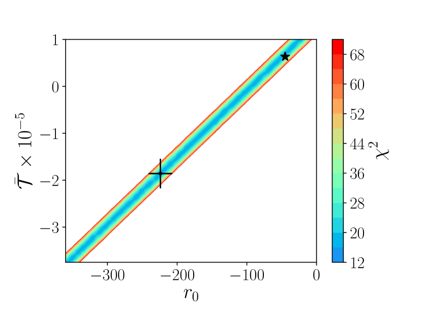
(c) Heat map for $\Delta E_{4}$-fit to order $L^{-6}$
without priors; $a_{0}$ is fixed to 0.434.

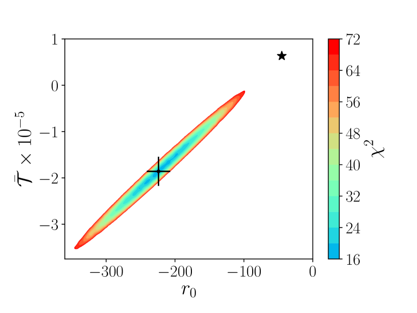
(d) Heat map for $\Delta E_{4}$-fit to order $L^{-6}$
with priors, cf. Tab. 5; $a_{0}$ is fixed to 0.434.

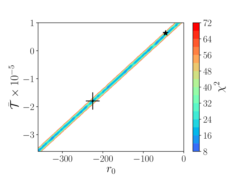
(e) Heat map for $\Delta E_{5}$-fit to order $L^{-6}$
without priors; $a_{0}$ is fixed to 0.433.

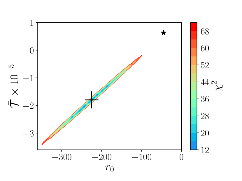
(f) Heat map for $\Delta E_{5}$-fit to order $L^{-6}$
with priors, cf. Tab. 5; $a_{0}$ is fixed to 0.433.

Figure 13: $\chi^{2}$ heat maps a) to f) that correspond to the fits with EC as well as RC in the interval $[9,24]$ for $L$. The black data points with error bars mark the respective results for $r_{0}$ and $\bar{\mathcal{T}}$ from prior constrained fits, cf. Tab. 5. The black stars correspond to the perturbative predictions, calculated from the fixed $a_{0}$ values by using Eqs. (121) and (122).

References

- (1) S. R. Beane, W. Detmold, T. C. Luu, K. Orginos, M. J. Savage and A. Torok, Multi-Pion Systems in Lattice QCD and the Three-Pion Interaction, Phys. Rev. Lett. 100 (2008) 082004 [0710.1827].
- (2) B. Hörz and A. Hanlon, Two- and three-pion finite-volume spectra at maximal isospin from lattice QCD, 1905.04277.
- (3) C. Culver, M. Mai, R. Brett, A. Alexandru and M. Döring, Three pion spectrum in the channel from lattice QCD, Phys. Rev. D 101 (2020) 114507 [1911.09047].
- (4) M. Fischer, B. Kostrzewa, L. Liu, F. Romero-López, M. Ueding and C. Urbach, Scattering of two and three physical pions at maximal isospin from lattice QCD, 2008.03035.
- (5) T. D. Blanton, F. Romero-López and S. R. Sharpe, three-pion scattering amplitude from lattice QCD, 1909.02973.
- (6) M. T. Hansen, R. A. Briceño, R. G. Edwards, C. E. Thomas and D. J. Wilson, The energy-dependent scattering amplitude from QCD, 2009.04931.
- (7) A. Alexandru, R. Brett, C. Culver, M. Döring, D. Guo, F. X. Lee et al., Finite-volume energy spectrum of the system, 2009.12358.
- (8) T. D. Lee, K. Huang and C. N. Yang, Eigenvalues and Eigenfunctions of a Bose System of Hard Spheres and Its Low-Temperature Properties, Phys. Rev. 106 (1957) 1135.
- (9) K. Huang and C. Yang, Quantum-mechanical many-body problem with hard-sphere interaction, Phys. Rev. 105 (1957) 767.
- (10) T. T. Wu, Ground State of a Bose System of Hard Spheres, Phys. Rev. 115 (1959) 1390.
- (11) M. Lüscher, Volume Dependence of the Energy Spectrum in Massive Quantum Field Theories. 2. Scattering States, Commun.Math.Phys. 105 (1986) 153.
- (12) S. R. Beane, W. Detmold and M. J. Savage, n-Boson Energies at Finite Volume and Three-Boson Interactions, Phys. Rev. D76 (2007) 074507 [0707.1670].
- (13) W. Detmold and M. J. Savage, The Energy of n Identical Bosons in a Finite Volume at , Phys. Rev. D77 (2008) 057502 [0801.0763].
- (14) S. Tan, Three-boson problem at low energy and implications for dilute Bose-Einstein condensates, Phys. Rev. A 78 (2008) 013636 [0709.2530].
- (15) K. Polejaeva and A. Rusetsky, Three particles in a finite volume, Eur. Phys. J. A 48 (2012) 67 [1203.1241].
- (16) M. T. Hansen and S. R. Sharpe, Relativistic, model-independent, three-particle quantization condition, Phys. Rev. D90 (2014) 116003 [1408.5933].
- (17) M. T. Hansen and S. R. Sharpe, Expressing the three-particle finite-volume spectrum in terms of the three-to-three scattering amplitude, Phys. Rev. D92 (2015) 114509 [1504.04248].
- (18) H.-W. Hammer, J.-Y. Pang and A. Rusetsky, Three-particle quantization condition in a finite volume: 1. The role of the three-particle force, JHEP 09 (2017) 109 [1706.07700].
- (19) H. W. Hammer, J. Y. Pang and A. Rusetsky, Three particle quantization condition in a finite volume: 2. general formalism and the analysis of data, JHEP 10 (2017) 115 [1707.02176].
- (20) M. Mai and M. Döring, Three-body Unitarity in the Finite Volume, Eur. Phys. J. A53 (2017) 240 [1709.08222].
- (21) M. T. Hansen and S. R. Sharpe, Lattice QCD and Three-particle Decays of Resonances, 1901.00483.
- (22) S. Kreuzer and H.-W. Hammer, The Triton in a finite volume, Phys. Lett. B 694 (2011) 424 [1008.4499].
- (23) S. Kreuzer and H.-W. Hammer, On the modification of the Efimov spectrum in a finite cubic box, Eur. Phys. J. A 43 (2010) 229 [0910.2191].
- (24) S. Kreuzer and H.-W. Hammer, Efimov physics in a finite volume, Phys. Lett. B 673 (2009) 260 [0811.0159].
- (25) S. Kreuzer and H. W. Grießhammer, Three particles in a finite volume: The breakdown of spherical symmetry, Eur. Phys. J. A 48 (2012) 93 [1205.0277].
- (26) M. T. Hansen and S. R. Sharpe, Perturbative results for two and three particle threshold energies in finite volume, Phys. Rev. D93 (2016) 014506 [1509.07929].
- (27) M. T. Hansen and S. R. Sharpe, Threshold expansion of the three-particle quantization condition, Phys. Rev. D93 (2016) 096006 [1602.00324].
- (28) R. A. Briceño, M. T. Hansen and S. R. Sharpe, Relating the finite-volume spectrum and the two-and-three-particle matrix for relativistic systems of identical scalar particles, Phys. Rev. D95 (2017) 074510 [1701.07465].
- (29) S. R. Sharpe, Testing the threshold expansion for three-particle energies at fourth order in theory, Phys. Rev. D96 (2017) 054515 [1707.04279].
- (30) R. A. Briceño, M. T. Hansen and S. R. Sharpe, Numerical study of the relativistic three-body quantization condition in the isotropic approximation, Phys. Rev. D98 (2018) 014506 [1803.04169].
- (31) R. A. Briceño, M. T. Hansen and S. R. Sharpe, Three-particle systems with resonant subprocesses in a finite volume, Phys. Rev. D99 (2019) 014516 [1810.01429].
- (32) T. D. Blanton, F. Romero-López and S. R. Sharpe, Implementing the three-particle quantization condition including higher partial waves, JHEP 03 (2019) 106 [1901.07095].
- (33) R. A. Briceno, M. T. Hansen, S. R. Sharpe and A. P. Szczepaniak, Unitarity of the infinite-volume three-particle scattering amplitude arising from a finite-volume formalism, 1905.11188.
- (34) F. Romero-López, S. R. Sharpe, T. D. Blanton, R. A. Briceño and M. T. Hansen, Numerical exploration of three relativistic particles in a finite volume including two-particle resonances and bound states, JHEP 10 (2019) 007 [1908.02411].
- (35) M. T. Hansen, F. Romero-López and S. R. Sharpe, Generalizing the relativistic quantization condition to include all three-pion isospin channels, 2003.10974.
- (36) T. D. Blanton and S. R. Sharpe, Equivalence of relativistic three-particle quantization conditions, 2007.16190.
- (37) T. D. Blanton and S. R. Sharpe, Alternative derivation of the relativistic three-particle quantization condition, 2007.16188.
- (38) M. Döring, H. W. Hammer, M. Mai, J. Y. Pang, A. Rusetsky and J. Wu, Three-body spectrum in a finite volume: the role of cubic symmetry, Phys. Rev. D97 (2018) 114508 [1802.03362].
- (39) J.-Y. Pang, J.-J. Wu, H. W. Hammer, U.-G. Meißner and A. Rusetsky, Energy shift of the three-particle system in a finite volume, Phys. Rev. D99 (2019) 074513 [1902.01111].
- (40) J.-Y. Pang, J.-J. Wu and L.-S. Geng, system in finite volume, 2008.13014.
- (41) A. Jackura, S. Dawid, C. Fernández-Ramírez, V. Mathieu, M. Mikhasenko, A. Pilloni et al., Equivalence of three-particle scattering formalisms, Phys. Rev. D 100 (2019) 034508 [1905.12007].
- (42) M. Mikhasenko, Y. Wunderlich, A. Jackura, V. Mathieu, A. Pilloni, B. Ketzer et al., Three-body scattering: Ladders and Resonances, JHEP 08 (2019) 080 [1904.11894].
- (43) JPAC collaboration, A. Jackura, C. Fernández-Ramírez, V. Mathieu, M. Mikhasenko, J. Nys, A. Pilloni et al., Phenomenology of Relativistic Reaction Amplitudes within the Isobar Approximation, Eur. Phys. J. C79 (2019) 56 [1809.10523].
- (44) M. Mai and M. Döring, Finite-Volume Spectrum of and Systems, Phys. Rev. Lett. 122 (2019) 062503 [1807.04746].
- (45) M. Mai, M. Döring, C. Culver and A. Alexandru, Three-body unitarity versus finite-volume spectrum from lattice QCD, 1909.05749.
- (46) A. W. Jackura, R. A. Briceño, S. M. Dawid, M. H. E. Islam and C. McCarty, Solving relativistic three-body integral equations in the presence of bound states, 2010.09820.
- (47) S. M. Dawid and A. P. Szczepaniak, Bound states in the B-matrix formalism for the three-body scattering, 2010.08084.
- (48) HAL QCD collaboration, D. Kawai, S. Aoki, T. Doi, Y. Ikeda, T. Inoue, T. Iritani et al., scattering phase shift from the HAL QCD method with the LapH smearing, PTEP 2018 (2018) 043B04 [1711.01883].
- (49) HAL QCD collaboration, T. Doi, S. Aoki, T. Hatsuda, Y. Ikeda, T. Inoue, N. Ishii et al., Exploring Three-Nucleon Forces in Lattice QCD, Prog. Theor. Phys. 127 (2012) 723 [1106.2276].
- (50) D. Agadjanov, M. Döring, M. Mai, U.-G. Meißner and A. Rusetsky, The Optical Potential on the Lattice, JHEP 06 (2016) 043 [1603.07205].
- (51) J. Bulava and M. T. Hansen, Scattering amplitudes from finite-volume spectral functions, Phys. Rev. D100 (2019) 034521 [1903.11735].
- (52) P. Guo, M. Döring and A. P. Szczepaniak, Variational approach to -body interactions in finite volume, Phys. Rev. D98 (2018) 094502 [1810.01261].
- (53) P. Guo, Modeling few-body resonances in finite volume, 2007.12790.
- (54) P. Guo, Threshold expansion formula of bosons in a finite volume from a variational approach, Phys. Rev. D 101 (2020) 054512 [2002.04111].
- (55) S. König and D. Lee, Volume Dependence of N-Body Bound States, Phys. Lett. B 779 (2018) 9 [1701.00279].
- (56) P. Guo and V. Gasparian, Numerical approach for finite volume three-body interaction, Phys. Rev. D97 (2018) 014504 [1709.08255].
- (57) P. Guo and T. Morris, Multiple-particle interaction in (1+1)-dimensional lattice model, Phys. Rev. D99 (2019) 014501 [1808.07397].
- (58) F. Romero-López, A. Rusetsky and C. Urbach, Two- and three-body interactions in theory from lattice simulations, Eur. Phys. J. C78 (2018) 846 [1806.02367].
- (59) S. Beane et al., Charged multi-hadron systems in lattice QCD+QED, 2003.12130.
- (60) J. Gasser, V. E. Lyubovitskij and A. Rusetsky, Hadronic atoms in QCD + QED, Phys. Rept. 456 (2008) 167 [0711.3522].
- (61) L. Landau and E. Lifschits, Quantum Mechanics, vol. Volume 3 of Course of Theoretical Physics. Pergamon Press, Oxford, 2004.
- (62) N. Schlage, “Relativistic -particle energy shift in finite volume: auxiliary fits.” https://github.com/NikSchlage/phi4_auxiliary, 2020.
- (63) J. Gasser and H. Leutwyler, Light Quarks at Low Temperatures, Phys. Lett. B 184 (1987) 83.
- (64) M. Lüscher, Two particle states on a torus and their relation to the scattering matrix, Nucl.Phys. B354 (1991) 531.
- (65) K. Symanzik, Cutoff dependence in lattice theory in four-dimensions, NATO Sci. Ser. B 59 (1980) 313.
- (66) Jülich Supercomputing Centre, JUQUEEN: IBM Blue Gene/Q Supercomputer System at the Jülich Supercomputing Centre, Journal of large-scale research facilities 1 (2015) .
- (67) Jülich Supercomputing Centre, JURECA: Modular supercomputer at Jülich Supercomputing Centre, Journal of large-scale research facilities 4 (2018) .
- (68) Jülich Supercomputing Centre, JUWELS: Modular Tier-0/1 Supercomputer at the Jülich Supercomputing Centre, Journal of large-scale research facilities 5 (2019) .
- (69) R Core Team, R: A Language and Environment for Statistical Computing. R Foundation for Statistical Computing, Vienna, Austria, 2019.
- (70) B. Kostrzewa, J. Ostmeyer, M. Ueding and C. Urbach, “hadron: package to extract hadronic quantities.” https://github.com/HISKP-LQCD/hadron, 2020.