Neglected X-ray discovered polars: III. RX J0154.0–5947, RX J0600.5–2709, RX J0859.1+0537, RX J0953.1+1458, and RX J1002.2–1925

We report results on the ROSAT-discovered noneclipsing short-period polars RX J0154.0-5947, RX J0600.5-2709, RX J0859.1+0537, RX J0953.1+1458, and RX J1002.2-1925 collected over 30 years. We present accurate linear orbital ephemerides that allow a correct phasing of data taken decades apart. Three of the systems show cyclotron and Zeeman lines that yield magnetic field strengths of 36 MG, 19 MG, and 33 MG for the last three targets, respectively. RX J0154.0-5947, RX J0859.1+0537, and RX J1002.2-1925 show evidence for part-time accretion at both magnetic poles, while RX J0953.1+1458 is a polar with a stable one-pole geometry. RX J1002.2-1925 shows large variations in the shapes of its light curves that we associate with an unstable accretion geometry. Nevertheless, it appears to be synchronized. We determined the bolometric soft and hard X-ray fluxes and the luminosities at the Gaia distances of the five stars. Combined with estimates of the cyclotron luminosities, we derived high-state accretion rates that range from $\dot{M}\!=\!2.9\!\times\!10^{-11}$$M_{\odot}$yr^-1 to $9.7\!\times\!10^{-11}$$M_{\odot}$yr^-1 for white dwarf masses between 0.61 and 0.82 $M_{\odot}$, in agreement with predictions based on the observed effective temperatures of white dwarfs in polars and the theory of compressional heating. Our analysis lends support to the hypothesis that different mean accretion rates appply for the subgroups of short-period polars and nonmagnetic cataclysmic variables.

1 Introduction

The discovery of hard and soft X-ray emission and of strong circular polarization of the close binaries AM Her, VV Pup, and AN UMa (Hearn & Richardson, 1977; Tapia, 1977) identified them as a very distinct type of object, for which Krzeminski & Serkowski (1977) proposed the name “polar”. They contain a mass-losing late-type main-sequence star and an accreting magnetic white dwarf (WD) in synchronous rotation. Of the more than 1200 cataclysmic variables (CVs) in the catalog of Ritter & Kolb (2003, final online version 7.24 of 2016,) 114 are confirmed polars. Many of these were discovered by their X-ray emission, which dominates the bolometric luminosity in high accretion states. The basic physical mechanism underlying the hard and soft X-ray emission was described by Fabian et al. (1976), King & Lasota (1979), and Lamb & Masters (1979). Increasing the still moderate number of well-studied polars will shed light on incompletely understood aspects of the physics of accretion (Bonnet-Bidaud et al., 2015; Busschaert et al., 2015), close binary evolution (Knigge et al., 2011; Belloni et al., 2020), the origin of magnetic fields in CVs (Briggs et al., 2018; Belloni & Schreiber, 2020), and the complex magnetic field structure of accreting WDs (Beuermann et al., 2007; Wickramasinghe et al., 2014; Ferrario et al., 2015).

Our optical identification program of high-galactic latitude soft ROSAT X-ray sources led to the discovery of 27 new polars (Thomas et al., 1998; Beuermann et al., 1999; Schwope et al., 2002). Twenty sources have been described in previous publications. In this series of three papers, we describe the remaining seven sources. In Papers I and II, we presented comprehensive analyses of V358  Aqr (= RX J2316.1–0527) (Beuermann et al., 2017, Paper I) and of the eclipsing polar HY Eri (= RX J0501.7–0359) (Beuermann et al., 2020, Paper II). Here, we present shorter analyses of the remaining five sources RX J0154.0–5947, RX J0600.5–2709, RX J0859+0536, RX J0953+1458, and RX J1002–1925 that are all noneclipsing. Our results include accurate long-term orbital ephemerides that permit the correct phasing of observations taken decades apart.

Table 1: Short names, epoch 2000 coordinates, high-state $V$-band magnitude, orbital period, and Gaia distance with 90% confidence errors.

Short	Optical position			$V$	$P_{\mathrm{orb}}$	$d_{\mathrm{\,Gaia,DR2}}$
Name	RA,DEC (2000)		l, b	high	(min)	(pc)
J0154	01 54 00.9	–59 47 49	$289.0,-55.6$	15	88.95	$320\,^{+4}_{-3}$
J0600	06 00 33.3	–27 09 19	$233.0,-22.5$	19	78.69	$1138\,^{+621}_{-325}$
J0859	08 59 09.2	+05 36 54	$223.2,+30.9$	17	143.93	$437\,^{+32}_{-28}$
J0953	09 53 08.2	+14 58 36	$220.0,+46.9$	17	103.71	$448\,^{+61}_{-48}$
J1002	10 02 11.7	–19 25 37	$257.0,+28.0$	17	99.98	$797\,^{+93}_{-67}$

Table 2: Journal of X-ray observations (Cols. 1–6), interstellar extinction (Cols. 7–9), and the results of X-ray spectral fits with the sum of a multitemperature thermal component and a single-blackbody soft X-ray component with k$T_{\mathrm{bb1}}$ (Cols. 10–12). The bolometric flux in Col. (11) is three times that of the single-blackbody fit (see Sect. 3.1). The cyclotron flux in Col. (13) is an estimate based on nonsimultaneous data. The luminosities in Cols. (14–16) are calculated with the Gaia distances in Table 1. The luminosity ratio in Col. (17) is $R_{\mathrm{L}}\!=\!L_{\mathrm{sx}}/(L_{\mathrm{hx}}+L_{\mathrm{cyc}})$. The blackbody temperatures in Col. (10) are quoted with errors. The errors are omitted for the derived parameters in Cols. (12-20). The accretion rates in Cols. (18) and (19) were calculated for the WD mass in Col. (20). Abbreviations: RASS = ROSAT All Sky Survey with the PSPC as detector, R = ROSAT pointed mode, X = XMM-Newton, P = PSPC as detector, H = HRI, pn = EPIC camera with pn as detector, M = MOS1&2, hi = high state, in = intermediate state, and lo = low state. Numbers in brackets indicate errors in the last digits. A colon indicates an uncertain value.

(1)	(2)	(3)		(4)	(5)	(6)	(7)	(8)	(9)	(10)	(11)	(12)	(13)	(14)	(15)	(16)	(17)	(18)	(19)	(20)
Short	Start date	Instr.		Exp.	$CR$	$HR1$	$N_{\mathrm{H,gal}}$	$N_{\mathrm{H,E_{B-V}}}$	$N_{\mathrm{H,ad}}$	k$T_{\mathrm{bb1}}$	$f_{\mathrm{sx,bol}}$	$f_{\mathrm{th,bol}}$	$f_{\mathrm{cyc}}$	$L_{\mathrm{sx}}\leavevmode\nobreak\ \leavevmode\nobreak\ \leavevmode\nobreak\$	$L_{\mathrm{hx}}\leavevmode\nobreak\ \leavevmode\nobreak\ \leavevmode\nobreak\$	$L_{\mathrm{cyc}}$	$R_{\mathrm{L}}$	$\dot{M}_{\mathrm{x}}$	$\dot{M}_{\mathrm{x+cyc}}$	$M_{1}$
Name		State		(s)	(1/s)		($10^{20}$ H-atoms/cm2)			(eV)	$(10^{-11}$erg/cm2s)			($10^{32}$ erg/s)				($10^{-11}\!M_{\odot}$/yr)		($M_{\odot}$)
J0154	26 Nov 1990	RASS	hi	138	0.346	$-0.78$	1.96	1.0 (5)	1.0	$24^{+3\leavevmode\nobreak\ }_{-3}$	$3.82$	0.251)	0.50	1.76	0.23	0.46	2.55	$2.3$	2.9	0.75:
	1 Jul 1992	R P	in	5158	0.101	$-0.57$			1.0	$24^{+3\leavevmode\nobreak\ }_{-3}$	$0.76$	0.201)	0.10	0.35	0.18	0.10	1.27	$0.6$	0.7	0.75:
	3 Jan 1995	R H	hi	11248	0.080
	1 May 2002	X pn	lo	5040	0.005
J0600	10 Sep 1990	RASS	hi	574	0.520	$-0.92$	2.20	1.5 (5)	1.5	$42^{+8\leavevmode\nobreak\ }_{-7}$	$2.20^{2)}$	0.202)	0.08	$6.53^{2)}$	$1.19^{2)}$	$0.47^{2)}$	3.93	$9.1^{2)}$	$9.7^{2)}$	0.75:
	12 Sep 1995	R H	lo	13474	0.002
J0859	28 Okt 1990	RASS	hi	368	0.3003)	$-0.86$	3.79	3.1 (8)	2.8	$38^{+10}_{-8}$	3.26	0.191)	0.50	2.79	0.33	0.86	2.36	5.4	6.9	0.61
	24 Apr 1996	R H	in	32846	0.0223)
J0953	7 Nov 1990	RASS	hi	335	0.4303)	$-0.72$	3.11	2.2 (6)	2.2	$46^{+9\leavevmode\nobreak\ }_{-8}$	1.99	0.561)	0.40	1.79	0.56	0.72	1.04	4.6	5.8	0.63
	31 May 1996	R H	in	4977	0.0233)
J1002	22 Nov 1990	RASS	hi	474	0.6903)	$-0.97$
	16 Nov 1992	R P	lo	4192	$-0.0002$
	30 Nov 1993	R P	hi	1609	0.7083)	$-0.93$	3.96	2.9 (9)	$\ga\!1.0$	$\la\!50$	$1.78^{4)}$	0.224)	0.434)	$5.07^{4)}$	$1.25^{4)}$	2.464)	1.37	6.34)	$8.7^{4)}$	0.82
	4 Jun 1995	R H	hi	12474	0.120
	10 Dec 2001	X pn	in	3160			3.96	2.9 (9)	$\ga\!1.0$	$\la\!50$	$0.86^{4)}$	0.274)	0.134)	$2.45^{4)}$	$1.54^{4)}$	0.744)	1.08	4.04)	$4.7^{4)}$	0.82
		X M	in	5820

1) Fit with $N_{\mathrm{H,int}}$ = 0.   2) Lower limit based on $d\,\geq\,813$ pc. 3) Mean of bright phase.   4) Lower limits based on $N_{\mathrm{H}}$$\,\geq\,1.0\!\times\!10^{20}$ H-atoms cm^-2.

Table 3: Journal of time-resolved spectroscopic observations.

Short Name	Date	Wavelength	Res.	Number	Exp.	Tel.
		(Å)	(Å)	spectra	(s)
J0154–59	23 Aug 1993	3500–9500	10	6	600	(1)
	17 Dec 1993	3500–9500	8	18	480	(2)
	3–5 Jul 1995	3500–5400	6/8	21	420	(1,4)
	24–25 Nov 1995	3800–9119	10	35	300	(1)
J0600–27	16 Nov 1995	3600–10200	15	1	1800	(1)
	4 Mar 1997	3600–10200	15	9	900	(1)
J0859+05	13 Dec 1993	3500–9200	20	1	1200	(1)
	5–7 Feb 1995	3810–5556	6	140	trailed	(3)
	5–7 Feb 1995	5560–9200	6	150	trailed	(3)
	7–8 Feb 1995	4173–5071	1.6	54	trailed	(3)
J0953+14	13 Dec 1993	3500–9200	20	1	1200	(1)
	5–7 Feb 1995	3810–5556	6	66	trailed	(3)
	5–7 Feb 1995	5560–9200	6	78	trailed	(3)
J1002–19	24 Dec 1992	3600–9120	15	1	1800	(1)
	26 Dec 1992–1 Jan 1993	3500–5389	6	21	600	(1)
	1 Mar 1997	3300–10500	15	11	600	(1)
	2 Mar 1997	4070–7200	6	10	600	(1)

(1) ESO/MPI 2.2-m EFOSC2, (2) ESO 1.5m B and C spectrograph, (3) Calar Alto 3.5m TWIN, trailed spectra, exposure times $25\!-\!60$ min, (4) spectral resolution 6 A for 1$\aas@@fstack{\prime\prime}$0 slit width, and 8 A for 1$\aas@@fstack{\prime\prime}$5.

Table 4: Journal of time-resolved photometric observations.

Short Name	Dates	No. of	Total	Bands	Exp.	Tel.
		nights	hours		(s)
J0154–59	16–17 Sep 1993	2	6.3	V	150	(1)
	8–9 Jul 1995	2	6.4	V	120	(2)
	29–31 Aug 2015	2	5.5	Sloan r	120	(3)
	1–3 Sep 2015	2	5.6	grizJHK	90	(3)
	May 2016–Oct 2018	22	39,9	WL	60	(4)
J0600–27	5 Feb 1995		4.7	V+WL	300	(1)
	Sep 2017–Jan 2019	30	53.9	WL	60	(4)
J0859+05	15 Jan 1996		9.0	V	30	(1)
	Feb 2010–Jan 2015	22	38.1	WL	60	(5)
	Feb 2018–Jan 2019	7	12.2	WL	60	(4)
J0953+14	4 Feb 1995		7.5	V	240	(1)
	19 Mar 2002		7.0	WL	180	(6)
	Jan 2010–Feb 2015	14	19.4	WL	60	(5)
	Feb 2018–Jan 2019	5	8.6	WL	60	(4)
J1002–19	1 Feb 1995		2.0	V	150	(1)
	Feb 2010–Feb 2015	11	25.6	WL	60	(5)
	Jun 2016–Jan 2019	16	42.3	WL	60	(4)

(1) ESO / Dutch 90 cm, (2) ESO / Danish 1.5 m,  (3) MPI / ESO 2.2 m, GROND, (4) MONET / S 1.2 m, (5) MONET / N 1.2 m, and (6) Observatorio Astronómico de Mallorca, 30 cm; WL = white light.

2 Observations

In Table 1 we summarize characteristic parameters of our targets such as the positions of the optical counterparts, the high-state $V$-band magnitude, the orbital periods derived in this paper, and trigonometric distances from the Gaia DR2 (Gaia Collaboration, Brown et al., 2018; Bailer-Jones et al., 2018). Finding charts were acquired from the PanSTARRS data archive (Chambers et al., 2016) and are provided in Appendix B.

2.1 X-ray observations

All targets discussed in this paper were discovered as variable very soft high galactic latitude X-ray sources in the ROSAT All Sky Survey (RASS) and observed subsequently with ROSAT in the pointed phase. The RASS covered the entire sky within one half year, starting in July 1990. Any target within its actual viewing strip was visited every 96 min for an exposure time of up to 30 s. All X-ray observations of our targets are summarized in Cols. 1–6 of Table 2. Columns 7–9 contain information on the interstellar extinction, and Cols. 10–12 list results of the X-ray spectral fits that are discussed in turn below. The hardness ratio $HR1$ in Col. 7 refers to the ROSAT observations with the Position-Sensitive Proportional Counter (PSPC) as detector. The PSPC was sensitive from $0.10\!-\!2.4$ keV, with two windows from $0.1\!-\!0.28$ keV (pulse height channels 11-41) and $\sim\!0.5\!-\!2.0$ keV (pulse height channels 51-201), which define the count rates $S$ and $H$ in the soft and hard bands, respectively. The hardness ratio was defined as $HR1\!=\!(H\!-\!S)/(H\!+\!S)$. The PSPC spectra of the polars in this paper are dominated by soft X-rays and have large negative $HR1$. Subsequent pointed ROSAT observations were made with the PSPC or, after its shutdown due to the small amount of counter gas left, with the High Resolution Imager (HRI). The HRI lacked energy resolution and was less sensitive than the PSPC, but had a higher spatial resolution and an even lower background. Some information on the relative response of PSPC and HRI and on the energy flux per PSPC unit count rate are given in Appendix A. An additional observation with XMM-Newton and the pn and MOS detectors of the EPIC camera is available for J1002 (Ramsay & Cropper, 2003).

2.2 Optical spectrophotometry

Time-resolved spectrophotometry was acquired between 1992 and 1997, using the ESO 1.5 m telescope at La Silla in Chile with the Boller and Chivens

spectrograph and the ESO/MPI 2.2 m telescope with EFOSC2. The spectra were taken with different spectral resolutions and wavelength coverage. We refer to spectra covering the entire optical range with a full width at half maximum (FWHM) of $10\!-\!20\AA$ as low resolution, spectra with reduced wavelength coverage and FWHM$\,\simeq\!6\AA$ as medium resolution, and with a FWHM$\,=\!1.6$Å as high resolution. Trailed simultaneous blue and red medium-resolution spectra of J0859 and J0953 were acquired with the TWIN spectrograph on the 3.5 m telescope of the Centro Astronomico Hispano Alemán Calar Alto, Spain. Table 3 summarizes the observations.

2.3 Optical photometry

Time-resolved photometry was acquired between 1993 and 2019. Details are provided in Table 4. Most of the data were taken in white light (WL), using the two robotic 1.2 m MONET telescopes, MONET/N at the University of Texas McDonald Observatory and MONET/S at the South African Astronomical Observatory. All images were corrected for dark current and flat-fielded in the usual way. All times were measured in UTC and converted into barycentric dynamical time (TDB), using the tool provided by Eastman et al. (2010) , which also accounts for the leap seconds. All times that enter the calculation of the ephemerides are listed in Appendix C.

As described in Paper I, we performed synthetic photometry in order to tie the WL measurements into the standard $ugriz$ system. We defined a MONET-specific WL AB magnitude $w$, which has its pivot wavelength $\lambda_{\mathrm{piv}}\!=\!6379$ Å in the Sloan $r$ band. For a wide range of incident spectra, the synthetic color $|(w\!-\!r)_{\mathrm{syn}}|\!\lesssim\!0.1$. Setting $w\!\simeq\!r$ is correct within 0.1 mag, except for very red stars.

3 General approach

All five targets were identified as polars by one or more of the following properties: (i) variable soft X-ray emission, (ii) optical spectroscopic and photometric variability, (iii) optical emission lines with skewed profiles caused by streaming motions, (iv) strong He ii$\lambda$4686 line emission indicating the presence of an XUV source, (v) cyclotron emission lines, and (vi) Zeeman absorption lines, both indicative of magnetic field strengths in the tens of MG regime, and (vii) long-term variations in the form of high and low states.

Observationally, a high state is characterized by intense soft X-ray emission and strong He II lines produced by photoionization. Physically, “high” refers to accretion rates adequate to drive the standard secular evolution of CVs. “Low” refers to low-level or to switched-off accretion. Living long-term $V$-band light curves of J0859, J0953, and J1002 are available from the monitoring program of Ritter CVs in the Catalina Sky Survey (Drake et al., 2009) .

3.1 Analyzing the X-ray data

In a high state, the bolometric luminosity $L_{\mathrm{bol}}$ of a polar is dominated by soft and hard X-ray emission. Our targets emit intense quasi-blackbody soft X-rays and thermal hard X-rays. The hard component originates from the post-shock cooling flow in competition with cyclotron emission. The peak temperature in the flow is about 30 keV (20 keV) for a WD of 0.75 $M_{\odot}$ (0.60 $M_{\odot}$) in a pure bremsstrahlung model with a shock near the WD surface, but lower for a tall shock or a strong magnetic field (Woelk & Beuermann, 1996; Fischer & Beuermann, 2001). Soft X-rays arise from the complex reprocessing of the energy carried into the WD atmosphere in the spot and its vicinity (Lamb & Masters, 1979; King & Lasota, 1979; Kuijpers & Pringle, 1982). The bolometric fluxes of both spectral components are difficult to measure because the XUV flux is severely degraded by interstellar extinction and effectively inaccessible below about 0.1 keV. Of the hard component, the ROSAT PSPC catches only a glimpse and the detectors of the EPIC camera on board XMM-Newton cover it still incompletely.

The soft component was conventionally modeled with a single blackbody with a temperature k$T_{\mathrm{bb1}}$. A model like this is a gross simplification, however, as shown by the highly resolved optically thick XUV spectrum of the prototype polar AM Her, taken with the Low Energy Transmission Grating Spectrometer (LETGS) on board Chandra. An improved model involves temperatures k$T_{\mathrm{bb}}$, ranging from about 0.5 to $2.0\,\times\,$k$T_{\mathrm{bb1}}$. In the case of AM Her, the single-blackbody fit underestimated the bolometric energy flux by a factor of $3.7\,\pm\,0.7$ (Beuermann et al., 2012, see their Table 1). This factor may well differ for individual polars, but in the absence of further information, we corrected the bolometric energy fluxes $f_{\mathrm{bb1,bol}}$ of our single-blackbody PSPC fits upward by a factor $c_{\mathrm{sx}}\!=\!3$ and treated the EPIC pn-spectrum in the same way. A separate problem in measuring $f_{\mathrm{bb1,bol}}$ from PSPC spectra is the tradeoff between the blackbody temperature k$T_{\mathrm{bb1}}$ and the interstellar absorbing column density $N_{\mathrm{H}}$ in front of the source, which leads to large correlated errors in the fit parameters. This problem is relaxed by recent progress in the construction of 3D models of the galactic extinction $E_{\mathrm{B-V}}$ (e.g., Schlafly & Finkbeiner, 2011; Lallement et al., 2018), the conversion of $E_{\mathrm{B-V}}$ into $N_{\mathrm{H}}$ (Nguyen et al., 2018), and the availability of Gaia distances (Gaia Collaboration, Brown et al., 2018; Bailer-Jones et al., 2018). Combined, they allow an educated guess of $N_{\mathrm{H}}$ that may be more trustworthy than the result of a free PSPC fit, except for particularly well-exposed PSPC spectra.

In addition to absorption by interstellar gas, the emerging X-rays may suffer internal absorption by atmospheric and infalling matter, which we assume only affects the hard X-ray component. The internal absorber probably fluctuates in space and time, a situation that is only approximately described by the concept of a partial absorber with a covering fraction $f_{\mathrm{pc}}$ and an unabsorbed fraction $1-$$f_{\mathrm{pc}}$. Because the quality of the PSPC spectra is only moderate, we opted for a simple model that includes (i) a multitemperature thermal hard X-ray component with an added partial-absorber feature and (ii) a single-blackbody soft X-ray component with the energy flux corrected upward by $c_{\mathrm{sx}}\!=\!3$. The thermal component approximates a cooling-flow model by including a Mekal or bremsstrahlung component with a fixed high temperature of 20 keV and one or two fitted low-temperature Mekal components with temperatures between 0.2 and 2 keV. For consistency reasons, we adopted the same simple model for the single XMM EPIC pn spectrum we considered. Our own more complex cooling-flow model (Beuermann et al., 2012) did not give significantly different integrated energy fluxes. The fits to the ROSAT PSPC spectra are not sensitive to different levels of internal absorption, while the fit to the XMM-Newton EPIC pn spectrum of J1002 improves substantially when internal absorption is added, as noted already by Ramsay & Cropper (2003).

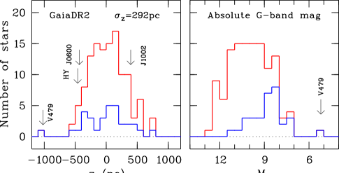
Figure 1: Left: Frequency distribution of polars perpendicular to the galactic plane based on the distances in the Gaia DR2 for the stars listed in the final 2016 version 7.24 of the catalog of Ritter & Kolb (2003). The red histogram shows all polars, and the blue histogram shows long-period systems with $P_{\mathrm{orb}}$$\,>\!0.12$ d. Right: Distribution of the absolute G-band magnitude. Arrows indicate individual objects discussed in the text.

3.2 Distances, scale height, and luminosities

Part of this study was facilitated by the availability of Gaia DR2 distances for practically all known polars (Gaia Collaboration, Brown et al., 2018; Bailer-Jones et al., 2018). We show in Fig. 1, the frequency distribution of polars as a function of the separation $z\!=\!d\,\mathrm{sin}\,b$ from the Galactic plane, with $d$ the distance and $b$ the galactic latitude, for systems listed in the final 2016 online version 7.24 of the catalog of Ritter & Kolb (2003). In Paper II and in the present paper, we found that HY Eri, J0600, and J1002reside at $\mid\!z\!\mid\,\simeq\!400$ pc, raising the question whether they might be halo objects. The three objects are marked by arrows in the left panel of Fig. 1, and we conclude that their distances from the plane are entirely compatible with their being members of what may be a single population of polars. Its standard deviation is $\sigma_{\mathrm{z}}\!=\!292$ pc; the possible long-period polar V479 And (González-Buitrago et al., 2013) was excluded. When the distribution is split into short-period and long-period polars, the standard deviations become 288 pc and 311 pc, respectively. These distributions may obviously be affected by an increasing incompleteness at higher $d$ and $\mid\!z\!\mid$. Nevertheless, the value of 288 pc is compatible with the scale heights of 260 pc and 280 pc for short-period magnetic CVs (mCVs) advocated by Pretorius et al. (2013) and Pala et al. (2020), respectively, but the value of 311 pc disagrees with the 120 pc assigned to young (i.e., long-period) systems by Pretorius et al. (2013). The right-hand panel shows the distribution of the Gaia DR2 absolute G-band magnitudes, which cluster between $M_{\mathrm{G}}\!=\!8$ and 12 and reflect the spread in in the luminosities caused by differences in the system parameters, notably the instantaneous accretion rate. Again, V479 And deviates from the well-defined sample of polars.

3.3 X-ray luminosity, accretion rate, and WD temperature

We calculated the bolometric luminosity of component $x$ as $L_{\mathrm{x,bol}}\!=\!\eta\,\pi d^{2}f_{\mathrm{x,bol}}$, where $d$ is the distance, $f_{\mathrm{x,bol}}$ the respective bolometric energy flux, and $\eta$ is a geometry factor, which is $\eta\,=\,4$ for isotropic emission. For a plane surface element that is viewed at an angle $\theta$, the geometry factor is $\eta\!=\!1/\mathrm{cos}\,\theta$. Because $\theta$ is only approximately known, we used a conservative mean $\eta\!=\!1.5$, although Heise et al. (1985) argued for an ’emitting mound’ with $\eta\,\simeq\,2$ (see also the $\eta$-values in Table 2 of Beuermann et al. 2012). We used $\eta\!=\!3$ for the thermal component, which accounts approximately for the X-ray albedo of the WD atmosphere, and $\eta\!=\!3$ for the beamed cyclotron radiation. With $c_{\mathrm{sx}}\!=\!3$ from above, we calculated the bolometric accretion-induced luminosity as

$$L_{\mathrm{bol}}\!\simeq\!\pi d^{2}(1.5\,c_{\mathrm{sx}}f_{\mathrm{bb1,bol}}+3f_{\mathrm{th,bol}}+3f_{\mathrm{cyc,bol}})\!\simeq\!\mathrm{G}M_{1}\dot{M}/R_{1}$$ (1)

and equated it to the gravitational energy released by matter accreted from infinity at a rate $\dot{M}$ by a WD of mass $M_{1}$ and radius $R_{1}$. We added the X-ray luminosity and an estimate of the cyclotron luminosity in an attempt to describe the accretion-induced luminosity. We disregarded the stream emission.

The effective temperature $T_{1}$ of a sufficiently old accreting WD is thought to be largely determined by compressional heating (Townsley & Gänsicke, 2009). This theory relates the equilibrium temperature $T_{\mathrm{eq}}$ to the long-term mean accretion rate $\langle\dot{M}\rangle_{\mathrm{10}}$ in units of $10^{-10}$ $M_{\odot}$yr^-1 by

$$T_{\mathrm{eq}}\!=\!14200\,\langle\dot{M}\rangle_{\mathrm{10}}^{1/4}\,(M_{1}/0.75M_{\mathrm{\odot}})\leavevmode\nobreak\ \leavevmode\nobreak\ \mathrm{K}.$$ (2)

We here derived the accretion rate $\dot{M}$ for a measured or adopted $M_{1}$ and quote the temperature $T_{1}$ the WD would have if $\dot{M}$ were identified with $\langle\dot{M}\rangle_{\mathrm{10}}$. We discuss to which extent the accretion rates derived by us fit into the general picture of short-period polars.

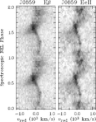
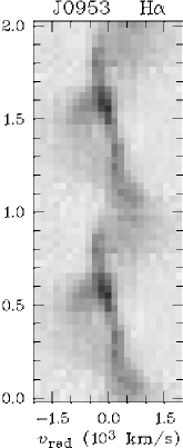
Figure 2: 2D representations of the phase-resolved He ii$\lambda$4686 and H$\beta$ spectra of J0859 (FWHM 1.6Å) and the H$\alpha$ spectra of J0953 (FWHM 6Å); the flux increases from white to black. The NEL component is prominent over one half of the orbit centered on the superior conjunction of the secondary star. The data are shown twice for better visibility of the orbital structure. The ordinate is spectroscopic phase with $\phi\!=\!0$ at the blue-red crossing of the NEL (see Sects. 6 and 7).

3.4 Ultraviolet and optical luminosity

No simultaneous X-ray and UV or optical observations are available for the present targets. We therefore constructed the UV-optical-IR spectral energy distributions (SED) from all available (nonsimultaneous) data in order to obtain an overview that would enable us to pick appropriate pairs of X-ray and optical flux levels. The upper envelope to the SED is taken as a measure of the UV-optical-IR flux in a high state of accretion. In favorable cases, the lower envelope provides information on the contributions by the stellar components. We collected the data using the Vizier SED tool provided by the Centre de Données astronomiques de Strasbourg. We searched the Galaxy Evolution Explorer (GALEX, Bianchi et al. 2017), the Sloan Digital Sky Survey (SDSS, Aguado et al. 2018), the Pan-STARRS Data Release 1 (Chambers et al., 2017), the SkyMapper catalog (Wolf et al., 2019), the Gaia catalog (Gaia Collaboration, Brown et al., 2018), the Two Micron All Sky Survey (2MASS, Skrutskie et al. 2006), the UKIRT Infrared Deep Sky Survey (UKIDSS, Lawrence et al. 2007), the VISTA Catalog (McMahon et al., 2013), the Wide-field Infrared Survey (WISE, Cutri et al. 2012,2014), the PPMXL catalog (Roeser et al., 2010), and the NOMAD catalog (Zacharias et al., 2005). Harrison & Campbell (2015) studied the light curves of our targets in the WISE W1 and W2 bands. SPITZER Space Telescope data of J0154 were discussed by (Howell et al., 2006).

3.5 System parameters

Polars display complex Balmer and helium emission lines. Schwope et al. (1997) distinguished three components, a narrow emission line (NEL) from the heated face of the secondary star, a broad base component (BBC) from the magnetically guided part of the accretion stream, and a high-velocity component (HVC) from the ballistic part of the accretion stream in the orbital plane. The small velocity dispersion of the NEL represents the distribution of emission from the static stellar atmosphere, while the widths of the two other components reflect the internal velocity variation of the accelerating stream. Fig. 2 shows the trailed spectra of the emission lines of He ii$\lambda$4686 and H$\beta$ in J0859 and of H$\alpha$ in J0953, taken on 7-8 and 5-7 February 1995, respectively. The lines are shown in the NEL (binary) phase with red-to-blue crossing at $\phi\!=\!0.5$. As expected for a sufficiently high inclination, the NEL is visible approximately from quadrature over superior conjunction to quadrature. The HVC crosses the NEL near spectroscopic phase 0.50. The fuzzy excursions to high positive and negative velocities result from the combined action of HVC and BBC. The NEL for the other three targets in our sample is well resolved in J1002, is perhaps marginally detected in J0154, and remains undetected in J0600. We measured the radial velocity for systems with resolved NEL by fitting a single Gaussian. For the combined BBC and HVC with its complex profile, we used the centroid of the cursor-defined full extent of the line near zero intensity, which suffices for our purpose because no quantitative argument is based on the measured broad-line velocities. For the two systems in which the NEL was not resolved, we measured radial velocities by fitting single Gaussians to the total line profiles.

The observed velocity amplitude $K_{2}^{\prime}$ of the NEL represents the centroid of the emission from the secondary star and its FWHM the distribution of the emission over the star. These need not be the same for the NEL of different species (e.g., Schwope et al., 2000). Transforming the observed $K_{2}^{\prime}$ into the velocity amplitude $K_{2}$ of the center of mass of the secondary star therefore requires a model of the emission in the respective line. There is evidence that metal lines with low-ionization potentials are best suited to trace the secondary star (Schwope et al., 2000; Beuermann & Reinsch, 2008; Beuermann et al., 2020). For this pilot study, we disregarded these complications and applied the irradiation model BR08 (Beuermann & Reinsch, 2008), which was devised for CaII$\lambda 8498$, also to the Balmer lines and to He ii$\lambda$4686. Using the inferred value of $K_{2}$ and a mass-radius relation $R_{2}(M_{2})$ of the Roche-lobe-filling secondary star, we calculated the system parameters as a function of the unknown inclination $i$. We used the radii of main-sequence stars of solar composition and an age of 1 Gyr of Baraffe et al. (2015, henceforth BHAC) for masses between 0.072 and 0.200$M_{\odot}$, represented by a power law $R_{\mathrm{BHAC}}/R_{\odot}\!=\!A\,(M_{2}/M_{\odot})^{B}$ with $A\!=\!0.831$ and $B\!=\!0.827$. Because the secondary stars in CVs are known to be more or less bloated, we set $R_{2}\!=\!R_{\mathrm{BHAC}}f_{123}$, where $f_{123}\!=\!f_{1}f_{2}f_{3}$ and $f_{1}\!=\!1.020$ accounts for expansion by magnetic activity and spot coverage, $f_{2}\!=\!1.045$ for tidal and rotational deformation of the Roche-lobe-filling star, and $f_{3}\!\geq\!1.0$ for the increased radius of a star driven out of thermal equilibrium (Knigge et al., 2011, and discussion in Paper II). Application of Kepler’s third law and Roche geometry (Kopal, 1959) yields the component masses as functions of $f_{3}$ and the inclination $i$ for a given $K_{2}^{\prime}$. With $R_{2}$ and $d$ known, the $i$-band magnitude of the secondary star is obtained, using the calibration of the $i$-band surface brightness $S_{\mathrm{i}}\!=\!i_{\mathrm{AB}}+5\,\mathrm{log}(R_{2}/R_{\odot}/d_{\mathrm{pc}}+1)$ that we established as a function of color or spectral type in Paper II. For spectral types dM4 to dM8 in steps of one subclass, $S_{\mathrm{i}}\!\simeq\!7.6$, 8.2, 8.7, 9.2, and $\sim\!10$. The expected spectral types of the secondaries are quoted by Knigge et al. (2011) in their Table 2. For the two of our objects that show the secondary star in their spectra, the observed $i$-band magnitudes and those predicted at the Gaia distance agree well.

None of the systems discussed in this paper is eclipsing, and obtaining information on $i$ is often based on circumstantial evidence. If the primary accretion spot at colatitude $\beta$ suffers a self-eclipse for a phase interval $\Delta\phi$, the angles $i$ and $\beta$ are related by

$$\mathrm{tan}\,i\,\mathrm{tan}\,\beta=1/\mathrm{cos}(\pi\Delta\,\phi).$$ (3)

The colatitude $\zeta$ of the field vector in the spot usually exceeds $\beta$ somewhat, but accounting quantitatively for the difference requires a closer study. The emitted cyclotron radiation is most intense perpendicular to and minimum along the field direction (cyclotron beaming). The cyclotron minimum is more than 10° wide, and we did not differentiate explicitely between $\zeta$ and $\beta$. The shape of the minimum may be modified by ff- and bf-absorption in the infalling matter. For $i\!>\!\beta$, a narrow absorption dip may occur when the line of sight crosses the magnetically guided part of the accretion stream, or a wide depression, when it is formed by an extended accretion curtain. The X-ray light curves are similarly shaped by geometric effects and photoabsorption.

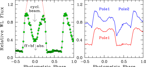
Figure 3: Left: WL light curve of the persistent one-pole system J0953 from Kanbach et al. (2008). The accretion spot is visible for 60% of the orbital period, and the central depression is created preferentially by cyclotron beaming. Right: Derived light curves depicting the effect of reduced beaming (red) and of adding a second accretion spot (blue). The latter mimics the light curves observed at times in J0859 and J1002.

3.6 Orbital light curves and ephemerides

The interpretation of the optical light curves of noneclipsing polars varies from simple to complex. As a simple case, we show in Fig. 3 (left panel) the binned WL light curve of the stable one-pole emitter J0953 observed by Kanbach et al. (2008). The accreting pole is visible between orbital phases $-0.30$ and $+0.30,$ and the light curve is shaped primarily by cyclotron beaming with a central minimum at the instant of closest approach of the line of sight to the accretion funnel, chosen here to define orbital phase $\phi\!=\!0$. The solid red curve shows the expected light curve formed by the varying aspect of the accretion spot without the beaming effect. Using the observed light curve (with its fluctuations) as a model, we constructed more complex cases. Increasing the minimum value of $\mid\!\beta-i\!\mid$ or the optical depth of the emission region reduces cyclotron beaming. An example is shown by the red curve in the right panel. Adding a second emission region in the lower hemisphere that is less influenced by beaming and is, for example, phase-shifted by 200° produces the blue curve, in which the three orbital minima can no longer uniquely be assigned to the two poles without independent information. Circular spectropolarimetry can provide the required information, as demonstrated for the case of HY Eri in Paper II, but is not available in the present study. The blue curve mimics the light curve 1996 V of J0859 in Fig. 6 and the light curves of 25 February 2018 and 13-14 December 2010 of J1002 in Fig. 8.

For each of our targets, we searched for an orbital feature that reliably marks the orbital period. A detected period was accepted as the orbital one if it agreed with the period of the radial-velocity variation, preferentially of the narrow component. The spectroscopic and photometric periods agreed in all cases within the uncertainties and all objects were accepted as synchronized polars, in part with tight margins for a possible remaining asynchronism. The errors of the derived orbital periods are sufficiently small to exclude alias periods over the time span of 30 yr, except for the faint object J0600, which exhibits a remaining uncertainty of one orbit in 150,000 cycles between 1995 and 2017.

We applied several methods to determine the timings of orbital features. These included sinusoidal fits to light curves, Gaussian fits to the fluxes around minima, and graphical methods. For instance, in double-humped light curves as that of J0953, we measured (i) the ingress to and egress from the bright phase individually, (ii) its center as the mean of the two timings, or (iii) the position of the central minimum and chose the one that displayed the smallest long-term scatter. We determined times of minima or maxima preferentially by the bisected-chord technique, marking the center between fall-off and rise at various intensity levels, and measuring the desired time and its error from the mean and the scatter of the markings. Our approach minimizes timing errors for objects whose light curves are distorted by flickering or noise.

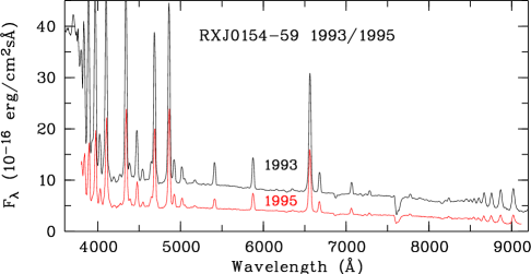
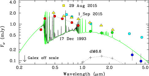
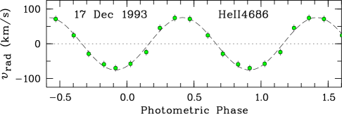
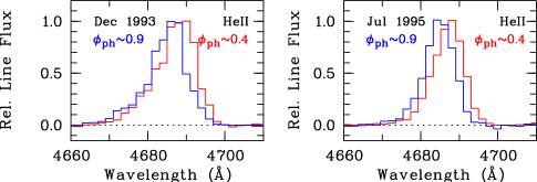
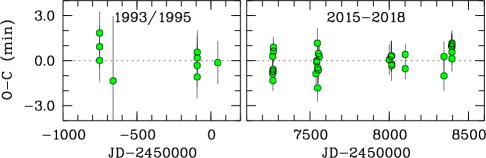
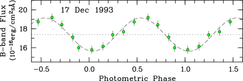
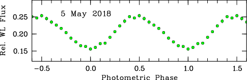
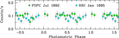
Figure 4: RX J0154.0–5947. Left, top: Mean spectra of of the observations on 23 August 1993 and 24 November 1995. Second from top: He ii$\lambda$4686 radial velocities obtained from the 17 December 1993 spectrophotometry with fitted sinusoid superimposed. Third from top: He ii$\lambda$4686 line profiles at maximum blueshift (blue curve) and redshift (red curve). Bottom: $O\!-\!C$ diagram for the times of orbital minimum. Right, top: Overall spectral energy distribution (see text). Bottom set of four panels: Spectral flux in the $B$ band of 17 December 1993 with peak magnitude $B\!=\!16.3$, Sloan $r$ light curve of 29 August 2015 with peak brightness $r\!=\!14.9$, WL relative flux on 5 May 2018, reaching magnitude $w\!=\!15.2$, and ROSAT X-ray light curves taken with the PSPC in the intermediate state of 1–2 July 1992 and with the HRI in the high state of 3–7 January 1995. All light curves are phased on the ephemeris of Eq. 4.

4 RX J0154.0–5947 (= J0154) in Hydrus

J0154 was discovered 1990 in the RASS as a moderately bright soft X-ray source, spectroscopically identified by us as a polar and listed as such in Beuermann & Thomas (1993), Beuermann & Burwitz (1995), and Beuermann et al. (1999). With up to $r\!=\!14.9$, it is the brightest star in our sample and with a Gaia distance of $d\!=\!320\,\pm\,4$ pc (Table 1) also the nearest.

4.1 X-ray observations

In the RASS, the star was detected with a PSPC count rate of $0.35\!\pm\!0.05$ cts s^-1 and a hardness ratio $HR1\!=\!-0.78\!\pm\!0.08$ (Table 2). In a pointed 5.1 ks PSPC observation of 1992, it was found at a reduced mean count rate of 0.10 PSPC cts s^-1 and an increased hardness ratio of $-0.57$, suggesting that only the soft component had weakened. In an 11.2 ks HRI observation on 3–7 January 1995, the system was found at a mean count rate of 0.080 HRI cts/s, which translates into about 0.64 PSPC cts s^-1 (Table 7), suggesting that the RASS observation represents only a moderate high state. The count rates of both observations in the bottom right-hand panel of Fig. 4 show little orbital variation. Phases are from Eq. 4. The visible pole of J0154 had nearly stopped accreting, when XMM-Newton barely detected it with 0.005(3) EPIC pn cts s^-1 on 1 May 2002 (Ramsay et al., 2004).

We fit the 1992 PSPC spectrum (not shown) with the X-ray spectral model described in Sect. 3.1. The fit gave k$T_{\mathrm{bb1}}$$\,=\!24$ eV, $N_{\mathrm{H}}$$\,=\!1.0\,\times\!10^{20}$ H-atoms cm^-2, and a blackbody flux $f_{\mathrm{bb1,bol}}$ that translates to $f_{\mathrm{sx,bol}}\!=\!c_{\mathrm{sx}}\,f_{\mathrm{bb1,bol}}\!=\!7.6\,\times\!10^{-12}$ (Table 2), with $c_{\mathrm{sx}}\!=\!3$ from Sect. 3.1. The reddening in front of the target is $E_{\mathrm{B-V}}$$\,\simeq\!0.011$ (Lallement et al., 2018) or about half the galactic value of 0.0195 (Schlafly & Finkbeiner, 2011), which corresponds to $N_{\mathrm{H}}$$\,=\!1.0\,\times\!10^{20}$ H-atoms cm^-2 (Nguyen et al., 2018), supporting the PSPC fit. In the brighter but statistically inferior RASS spectrum, the count rate of the soft component is higher by a factor of five, and the hard component remains about the same. For the same blackbody temperature of 24 eV, the soft X-ray flux in Table 2 is raised by a factor of five as well. A soft X-ray variability, exceeding that of the hard X-ray component, was seen also in other polars and taken as evidence for the concept of blobby accretion (Kuijpers & Pringle, 1982), which carries the kinetic free-fall energy into subphotospheric layers and releases the reprocessed energy as soft X-rays, independent of more tenuous sections of the flow that pass through a free-standing shock, radiating hard X-rays.

4.2 Orbital ephemeris

Time-resolved optical photometry of J0154 was performed over a time span of 25 yr. Its brightness was measured relative to a comparison star located at RA(2000)$\,=\!01^{\mathrm{h}}54^{\mathrm{m}}00\aas@@fstack{s}9$, DEC(2000)$\,=\!-59\degr 43\arcmin 33\arcsec$, or 0″ W and 256″ N of the target, which has $V\!=\!13.85$, $B\,-\,V\!=\!0.62$, Sloan $r\!=\!13.61$, and $w\,-\,r\!\simeq\!0.08$. All light curves of J0154 are characterized by a quasi-sinusoidal modulation with a period of 89 min (Fig. 4, lower right-hand panels). The star reached $r\!=\!14.9$ on 29 August 2015 and $w\!=\!15.2$ on 5 May 2018. Radial velocities measured from low-resolution spectra taken on 23 August and 17 December 1993 confirmed the photometric period as the orbital one (second left-hand panel from the top). ¿From 39 photometric minima of 1993, 1995, 2015, 2016, 2017, and 2018 (Table 9), we obtained the alias-free linear ephemeris

$$T_{\mathrm{min}}\!=\!\mathrm{TDB}\leavevmode\nobreak\ 2457263.76473(10)+0.061767741(3)\,E.\leavevmode\nobreak\ \leavevmode\nobreak\ \leavevmode\nobreak\$$ (4)

The $O\!-\!C$ diagram is shown in the lower left panel of Fig. 4. The tentative period $P_{\mathrm{orb}}\!=\!0\,\aas@@fstack{d}0556$ cited in the catalog of Ritter & Kolb (2003, final version 7.24 of 2016,) is not confirmed.

4.3 Spectrophotometry

Time-resolved low-resolution spectroscopy was collected on 23 August 1993, 17 December 1993, and on 24–25 November 1995. The top left panel shows the slightly smoothed mean low-resolution spectra of August 1993 and November 1995. They correspond to mean AB magnitudes $r\!=\!16.1$ and 16.9, respectively. The source displayed emission lines of H I, He I, He II, a strong Balmer jump in emission, and weak metal lines. No spectral features of the secondary star were detected. The large He ii$\lambda$4686 equivalent width with a ratio $W$(He ii$\lambda$4686)/$W$(H$\beta$)$\,\simeq\!0.79$ (Table 5) is typical of the high-state emission-line spectrum of a polar. The line profiles extend to $-1500$ and $+1000$ km s^-1, more in the Balmer than in the helium lines, but they are all peculiar in showing very little orbital variation. Single-Gaussian fits to lines observed in December 1993, July 1995, and November 1995 gave velocity amplitudes between 60 and 80 km s^-1, with very little variation in the phasing. The radial-velocity curve of the He ii$\lambda$4686 line in December 1993 is shown in the second left panel from the top in Fig. 4. The blue-to-red zero crossing for this line occurred at photometric phase $\phi_{\mathrm{br}}\!=\!0.164(15)$ in December 1993, at  0.17(2) in July 1995, and at 0.16(2) in November 1995. The H$\beta$ results are very similar. We show examples of the He ii$\lambda$4686 lines at maximum positive and negative excursion in Fig. 4 (third left panel from the top). The spectral resolutions between 6 and 10 Å did not suffice to identify the NEL component, although the variation in the line peak in 1993 may be an indication of its presence. Assuming that the line nevertheless relates to a fixed structure in the binary system (as the illuminated face of the secondary), these events define the spectroscopic or binary orbital period, $P_{\mathrm{sp}}\!=\!0\,\aas@@fstack{d}061767740(123)$. The period $P$ in Eq. 4, on the other hand, represents the rotational period of the WD. The difference is consistent with zero and limits any asynchronism to a level of $2\,\times\!10^{-6}$. Because identification of the NEL is required to locate the secondary star, it may be rewarding to study this bright system at higher spectral resolution.

4.4 Spectral energy distribution

Further insight into the properties of the system is obtained from the nonsimultaneous overall SED in the upper right-hand panel of Fig. 4, which shows the mean spectrum of August 1993 (black curve) along with a model spectrum (green curve) for an isothermal slab of hydrogen at a temperature of 17000 K, a pressure of $10^{3}$ dyne cm^-1, and a slab thickness of $10^{8}$ cm. The model fits the observed 1993 spectrum and is consistent with the 2MASS near-IR fluxes (green dots) and the Spitzer IRAC fluxes at 3.6 and 4.5 $\mu$m reported by Howell et al. (2006) (blue dots). We interprete this spectrum as the signature of a luminous accretion stream. There is no evidence for the associated accretion spot, however, which is evidently located on the far side of the white dwarf and is permanently out of view. On the other hand, our grizJHK photometry of August and September 2015 (yellow triangles and yellow square), photometry of SkyMapper (red), 2MASS (green), and Gaia 2, VISTA, and WISE (cyan blue) show higher fluxes that are probably associated with a spot on the near hemisphere that accretes only temporarily. Our optical and X-ray observations suggest that it was active in November 1990, July 1992, January 1995, and August and September 2015, but not in August and December 1993, July 1995, and May 2002. The persistent stream emission when the near spot is inactive explains the preponderance of negative radial velocities in the 1993 line profiles in Fig. 4 by the plasma motion toward the unseen pole.

The variability of the source is also indicated by the GALEX far-UV and near-UV fluxes of 0.050 mJy at 0.153 and 0.231 $\mu$m that belong to a low state, consistent with representing the WD. No spectral signature of the secondary star is detected.

4.5 System parameters

For $P_{\mathrm{orb}}$=89 min, the evolutionary sequence of Knigge et al. (2011) with $M_{1}\!=\!0.75$ $M_{\odot}$ predicts a Roche-lobe-filling secondary star with $M_{2}\!\simeq\!0.085$ $M_{\odot}$, $R_{2}\!\simeq\!0.132$ $R_{\odot}$, and spectral type dM6.6. For this spectral type, the $i$-band surface brightness of the secondary star is $S_{\mathrm{i}}\!\simeq\!9.0$ and its $i$-band magnitude becomes $i\!=\!20.9$ mag (0.016 mJy) for $d\!=\!320$ pc (Table 1). Its $K$-band magnitude would be 16.9 mag (0.116 mJy). The expected flux distribution of the secondary star is shown in the upper right-hand panel of Fig. 4 (crosses and dotted line). For the Knigge et al. component masses, the orbital velocity of the secondary star is $\upsilon_{2}\!=\!458$ km s^-1. For an assumed NEL amplitude of up to $\sim\!100$ km s^-1, interpreted by our irradiation model BR08 ($K_{2}/K_{2}^{\prime}\!=\!1.21$), the inclination does not exceed 15°. For a WD of 0.75  $M_{\odot}$, the secondary star is moderately bloated with $f_{3}\!=\!1.12$. As long as the inclination cannot be tightly constrained, similar models can be constructed with primary masses from $M_{1}\!=\!0.50$ up to the Chandrasekhar mass and inclinations between 20° and 12°. A promising path for progress involves a spectroscopic measurement of the WD radius, and thereby its mass, when J0154 lapses into a low state or a measurement of the inclination by the identification of the NEL.

The RASS soft and hard X-ray fluxes of Table 2 with the geometry factors of Sect. 3 give a high-state bolometric X-ray luminosity of $2.0\,\times\!10^{32}$ erg cm^-2s^-1 and an X-ray based accretion rate of $\dot{M}_{\mathrm{x}}\!=\!2.3\,\times\!10^{-11}$ $M_{\odot}$yr^-1 for an adopted WD mass of 0.75 $M_{\odot}$ (Table 2). The optical level of 1 September 2015 probably represents a high state as well, and we estimate that about $5.0\times\!10^{-12}$ erg cm^-2s^-1Å^-1 arises from cyclotron radiation. When it is included in the energy balance, the accretion rate rises to $\dot{M}_{\mathrm{x+cyc}}\!=\!2.9\,\times\!10^{-11}$ $M_{\odot}$yr^-1. If this rate equals the long-term mean, the expected WD temperature due to compressional heating would be 10400 K, near the lower end of the observed temperature range (Townsley & Gänsicke, 2009). Its 4600Å flux would be 0.040 mJy, close to the observed GALEX fluxes. In the 1995 HRI observation, the accretion rate could have reached $\dot{M}_{\mathrm{x+cyc}}\!\sim\!5\,\times\!10^{-11}$ $M_{\odot}$yr^-1.

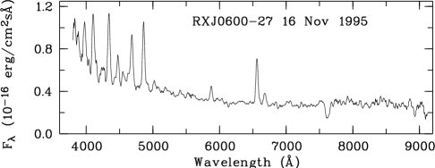
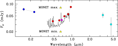
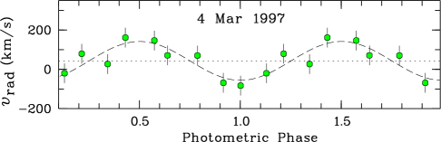
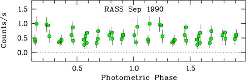
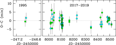
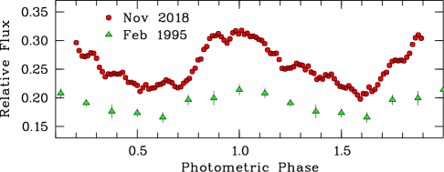
Figure 5: RX J0600.5–2709. Left, top: Identification spectrum taken on 16 November 1995. Left, center: Balmer line radial-velocity curve from phase-resolved spectroscopy on 4 March 1997. Left, bottom: $O\!-\!C$ diagram for orbital maxima (green) and minima (cyan). Right, top: Spectral energy distribution, showing the identification spectrum, and a summary of nonsimultaneous photometry (see text). Right, center: X-ray light curve taken in the RASS between 10 and 13 September 1990. Right, bottom: Light curves taken in WL on 5 February 1995 and 28 December 2018. The photometric phase is from Eq. 5.

5 RX J0600.5–2709 (= J0600) in Lepus

J0600 was discovered 1990 in the RASS as a bright and very soft X-ray source. The most distant and optically faintest object in our sample (Table 1) was spectroscopically identified by us as a polar and is listed as such in Beuermann et al. (1999). Its orbital period is close to the bounce period of CV evolution and its secondary is therefore close to substellar.

5.1 X-ray observations

In the RASS, J0600 was detected with a mean PSPC count rate of $0.52\!\pm\!0.03$ cts s^-1 and a hardness ratio of $HR1\!=\!-0.92\!\pm\!0.03$ (Table 1). The rather long exposure time of 568 s in 35 satellite visits allowed the construction of an orbital light curve, which shows no evidence for a periodicity. The center right panel of Fig. 5 shows the light curve folded over the orbital period of Eq. 5. Judged by the X-ray luminosity (Table 2), J0600 was in a high state during the RASS, and the lack of orbital modulation suggests that the accretion spot was permanently in view. In a 13.5 ks ROSAT HRI observation between 12 and 28 September 1995, it was found in a low state with a count rate of 0.0023 cts/s or a soft X-ray flux roughly a factor of 30 below that of the RASS.

The RASS PSPC spectrum (not shown) is dominated by soft X-rays and appears only moderately absorbed despite the large distance of J0600. No spectrally resolved follow-up X-ray observation is available. The unconstrained blackbody fit to the RASS spectrum prefers an unrealistic $N_{\mathrm{H}}$$\,\simeq\!0$ and k$T_{\mathrm{bb}}\!\simeq\!75$ eV with large errors (2RXS, Boller et al., 2016). At the position of J0600, the total extinction is $E_{\mathrm{B-V}}$$\,=\!0.0215$ (Schlafly & Finkbeiner, 2011) and the total neutral hydrogen column density is $N_{\mathrm{H}}$$\,=\!2.2\!\times\!10^{20}$ H-atoms cm^-2 (HI4PI Collaboration et al., 2016). The extinction in front of J0600 is $E_{\mathrm{B-V}}$ $=\!0.016\!\pm\!0.006$ (Lallement et al., 2018) and $N_{\mathrm{H}}$$\,=\!(1.5\!\pm\!0.5)\!\times\!10^{20}$ H-atoms cm^-2 (Nguyen et al., 2018). Adopting this value of $N_{\mathrm{H}}$, the PSPC fit with the X-ray spectral model of Sect. 3.1 yields $T_{\mathrm{bb}}$$\,=\!42$ eV and the X-ray fluxes and the accretion rate listed in Table 2. The Gaia distance for J0600 (Table 1) has a large error, and the luminosity and accretion rate are quoted for the 90% confidence lower limit of 813 pc and marked as lower limits.

5.2 Spectroscopy, photometry, and ephemeris

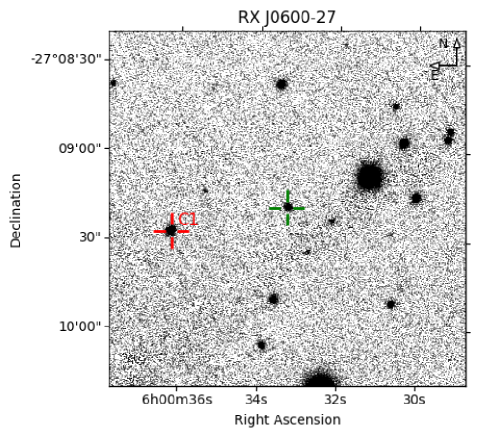
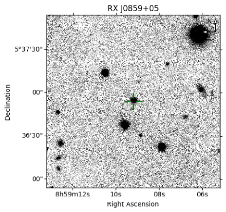
Figure 10: Left: Finding chart for RX J0600.5–2709. Size is 2′$\times$2′. The comparison star is 40″ E and 8″ S of the target and marked C1. Right: Finding chart for RX J0859.1+0537. Size is 2′$\times$2′. The comparison star is 15″ E and 162″ N of the target and outside the image.

The optical counterpart of J0600 was identified as a 19–20 mag periodically variable star in 4.7 h of WL photometry taken on 5 February 1995 with the ESO-Dutch 90 cm telescope. Its brightness was measured relative to a comparison star C1 that has AB magnitude $r\!=\!17.89$ and is located at RA(2000) = $06^{\mathrm{h}}00^{\mathrm{m}}36\aas@@fstack{\prime\prime}2$, DEC(2000) = $-27\degr 09\arcmin 27\arcsec$, 40″ E and 8″ S of the target (Fig. 10). The best period of the quasi-sinusoidal variation was 0 $\aas@@fstack{d}$ 0545(7) (Fig. 5, bottom right panel, green triangles). A low-resolution optical spectrum taken on 16 November 1995 with the ESO/MPI 2.2 m telescope at La Silla, Chile, revealed J0600 as a polar (top left panel). Strong He ii$\lambda$4686 emission with an equivalent-width ratio $W$(He ii$\lambda$4686)/$W$(H$\beta$)$\,=\!0.86$ (Table 5) indicated a high state of accretion. Further nine low-resolution spectra of 15 min exposure were taken on 4 March 1997, when the source was at a similar brightness level of $19\!-\!20$ mag. The emission-line radial velocities were measured by cross-correlating the individual spectra with the mean spectrum on a log $\lambda$ scale. The line profiles display the asymmetries characteristic of polars, but are not sufficiently well resolved to allow the separation of individual line components. The radial velocities in the left center panel of Fig. 5 yielded a period of $0\,\aas@@fstack{d}\,0535(35)$, revealing the photometric period as the orbital one and placing the star near the bounce period of CVs. The peak positive radial velocity occurs near photometric minimum. Except for the orbital modulation and the day-to-day variability by factors of two each, the optical counterpart to J0600 has shown little variability over the years. No optical equivalent to the 1995 X-ray low state was found. We derived a long-term ephemeris from the photometry of 5 February 1995 and WL photometry of 25 nights between September 2017 and January 2019 that resulted in 31 additional maximum and minimum times each. All times are reported in Table C in Appendix C. We fit the data by a linear ephemeris for the orbital maxima,

$$T_{\mathrm{max}}\!=\!\mathrm{TDB}\leavevmode\nobreak\ 2458015.55336(17)+0.054644792(10)\,E,\leavevmode\nobreak\ \leavevmode\nobreak\ \leavevmode\nobreak\$$ (5)

allowing for a shift of the minima relative to the maxima. The skewed light curves have their minima on average at $\phi\!=\!0.55$. There is no evidence for a deviation from linearity. Because of the 22-year hiatus between the two groups of timings, we cannot entirely exclude the nearest alias period on each side, which corresponds to an uncertainty of one in 151,194 cycles. These periods are separated by $+29.7$ ms and $-29.7$ ms from the period of Eq. 5, reaching a reduced $\chi^{2}_{\nu}\!=\!1.4$ and 2.0, respectively, relative to unity for the best period. The preliminary period $P_{\mathrm{orb}}\!=\!0\,\aas@@fstack{d}0757$ cited in the catalog of Ritter & Kolb (2003, final version 7.24 of 2016,) turned out to be incorrect.

5.3 Spectral energy distribution

The top right panel in Fig. 5 combines all available data into an SED that includes the low-resolution spectrum of the top left panel. The two yellow triangles indicate the full range of the MONET/S WL photometry, the blue dots the GALEX UV fluxes, the red dots fluxes from the Pan-STARRS DR1, and the cyan-blue ones the WISE W1 and W2 fluxes, all obtained via the VizieR photometry viewer. Haakonsen & Rutledge (2009) misidentified the 2MASS image of a bright star 26″ WNW with J0600 (Fig.10). The WISE images of the region show several faint sources near the target position, of which the brightest is located 7″ SW. Harrison & Campbell (2015) may have mistaken this 15 mag object for J0600. The 2MASS images show a faint equivalent to the WISE object, but no source at the position of J0600. The 3$\sigma$ upper limits are 0.15, 0.22, and 0.28 mJy in the $J,H$, and $K_{\mathrm{s}}$ bands, respectively, still permitting a broad hump that extends over the entire near-IR band. The hump looks suspiciously like the SED of a late M-dwarf, but the secondary star would be much fainter at the Gaia distance. A possible interpretation involves optically thick cyclotron emission in a magnetic field of $B\,\la\!20$ MG. The identification of the GALEX source with J0600 seems trustworthy because of the close positional coincidence. The origin of the UV emission remains uncertain. Phase-resolved observations in the different wavelength bands could resolve the open questions.

5.4 System parameters

Of all polars, only CV Hyi and V4738 Sgr (Burwitz et al., 1997) have orbital periods shorter than J0600. With less than 79 min, all three binaries fall below the bounce period $P_{\mathrm{bounce}}\!=\!81.8\pm 0.9$ min calculated by Knigge et al. (2011) for the evolution of the bulk of the (mostly nonmagnetic) CVs. A lower value would be obtained for a reduced braking efficiency, as may be appropriate for polars. The secondary mass at $P_{\mathrm{bounce}}$ is about 0.06 $M_{\odot}$ (Knigge et al., 2011), and as a given system evolves through this point, the accretion luminosity drops rapidly. The high observed X-ray luminosity of J0600 suggests that it is still approaching the minimum. The secondary is then expected to be a very late star or a brown dwarf. For example, a Roche-lobe-filling secondary of $M_{2}\!\simeq\!0.07$ $M_{\odot}$ with $f_{3}\!=\!1.15$ would have $R_{2}\!\simeq\!0.11$ $R_{\odot}$, a spectral type of dM8, and an $i$-band surface brightness $S_{\mathrm{i}}\!\simeq\!10$. For the 90% confidence lower limit to the distance of 813 pc, it would have $i\!\simeq\!24.3$ ($0.7\,\mu$Jy), and $K\!=\!19.6$ ($100\,\mu$Jy), which is far below the observed fluxes.

The narrow emission-line component could not be identified in J0600. When $K_{2}^{\prime}$ would tentatively be equated to the observed velocity amplitude of 99 km s^-1, this would imply an inclination of 14° for $M_{1}\!=\!0.75$$M_{\odot}$. Any primary mass between 0.5 $M_{\odot}$ and the Chandrasekhar limit can be accommodated.

The bolometric fluxes and luminosities of the X-ray components are listed in Table 2. When the cyclotron flux is included in the $\dot{M}$ calculation, the accretion rate rises for an 0.75 $M_{\odot}$ WD only minimally to $\dot{M}_{\mathrm{x+cyc}}\!\ga\!9.7\!\times\!10^{-11}$ $M_{\odot}$yr^-1, placing the star at the upper end of the range of accretion rates found in short-period polars (Townsley & Gänsicke, 2009). The equivalent equilibrium temperature of the WD would be 14100 K, implying a 4600 Å flux of the compressionally heated WD of 0.014 mJy, somewhat below the observed minimum MONET WL flux. Measuring the WD temperature and radius spectroscopically in a low state appears feasible.

Table 5: Equivalent widths of prominent emission lines in Å for the high-state spectra of Figs. 1 to 5. The letters b and f refer to the bright and faint orbital phase intervals, respectively.

Name	Date		H$\delta$	H$\gamma$	HeII	H$\beta$	HeII	HeI	H$\alpha$
					4686		5411	5876
0154-59	23 Aug 93		103.1	86.5	81.6	103.9	11.9	17.2	87.8
	17 Dec 93		111.6	102.5	78.5	99.6	15.1	20.6	89.4
	24 Nov 95		105.2	100.5	89.7	113.7	12.7	23.5	103.7
0600-27	16 Nov 95		45.7	57.8	47.7	55.6	6.7	17.7	62.3
0859+05	10 Jan 03		27.1	23.3	20.2	33.9	4.3	9.5	33.2
0953+05	6/7 Feb 95	b	11.2	11.4	3.4	13.0	1.0	3.8	12.7
		f	48.1	50.3	20.3	69.4	2.9	31.2	80.0
1002-19	24 Dec 92		12.8	9.0	15.9	17.0	3.4	2.8	25.1
	1 Mar 97	b	11.9	17.7	15.7	25.5	3.3	9.0	35.8
		f	32.6	47.9	50.7	47.9	9.9	13.0	68.4

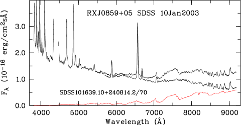
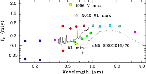
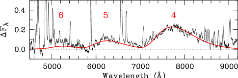
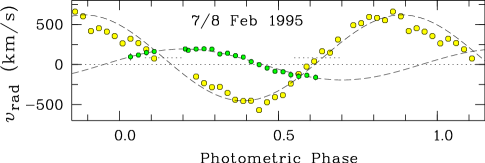
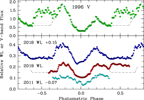
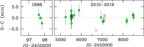
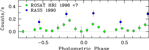
Figure 6: RX J0859.1+0537. Left, top: SDSS spectra of RXJ0859+05 (black curve) and the dM5 star SDSS J101639.10+240814.2 divided by 70 to match the TiO structures in the polar spectrum (red). The difference spectrum (black) shows faint cyclotron lines. Second from top: Model cyclotron spectrum (red) fit to the observed difference spectrum (black). Third from top: Mean radial-velocity curves of the NEL (green) and the combined BBC and HCV components (yellow) of H$\beta$, H$\gamma$, and He ii$\lambda$4686, measured from the high- and medium-resolution trailed spectra. Bottom: $O\!-\!C$ diagram for the times of the primary minimum. Green dots show this work, and open circles show results from Joshi et al. (2020) (see text). Right, top: Overall spectral energy distribution, built from nonsimultaneous data (see text). Center panels: V-band light curve of 15 January 1996 and WL light curves of on 4 March 2018, 17 January 2019, and 1 April 2011. The dashed lines schematically separate the emissions of the primary and the secondary pole. Bottom panel: Rosat X-ray light curves taken 1990 with the PSPC and 1996 with the HRI. Phases are from Eq. 6.

6 RX J0859.1+0537 (= J0859) in Hydra

J0859 was discovered 1990 in the RASS as a very soft X-ray source and was spectroscopically identified by us as a polar. It is listed as such in Beuermann et al. (1999). Its orbital period of 143.9 min, which places it at the lower edge of the remnant period gap of polars, as defined by Belloni et al. (2020) and Schwope et al. (2020).

6.1 X-ray observations

J0859 was detected in the RASS with a mean PSPC count rate of $0.27\!\pm\!0.03$ cts s^-1and a hardness ratio $HR1\,=\!-0.86\!\pm\!0.06$ (Table 2). Because the binary period of 144 min (Table 1) is commensurable with the 96 min ROSAT period, all satellite visits fall in three narrow orbital phase intervals. In a 32.8 ks HRI observation from 24 April to 12 May 1996, the source was detected with 0.010 HRI cts s^-1, equivalent to about 0.07 PSPC cts s^-1 (Table A.1 in Appendix A). This observation provided nearly complete phase coverage. The lower right-hand panel in Fig. 6 shows the two light curves, with the HRI count rate multiplied by a factor of seven. The X-ray and optical bright phases coincide and the central X-ray dip, near phase zero on the ephemeris of Eq. 6, probably marks the instance at which the line of sight to the WD passes through the magnetically guided part of the accretion stream. We define the soft X-ray flux in the bright phase by the two higher of the three RASS points with a mean of 0.30 PSPC cts s^-1. This value is entered into Col. (5) of Table 2 and is taken to represent the high state of J0859. The HRI observation of 1996 has a bright-phase count rate of 0.020 HRI cts s^-1, which converts into possibly as much as 0.14 PSPC cts s^-1 or half the RASS count rate, representing an intermediate state.

The only X-ray spectral information available is that of the RASS. A blackbody fit yields $T_{\mathrm{bb1}}\!\simeq\!38$ eV and $N_{\mathrm{H}}\!\simeq\!2.8\!\times\!10^{20}$ H-atoms cm^-2. The extinction in front of J0859 is $E_{\mathrm{B-V}}$$\,\simeq\!0.033\!\pm\!0.008$ (Lallement et al., 2018), about 3/4 of the total galactic extinction. The corresponding column density of cold matter is $N_{\mathrm{H}}$$\,=\!(3.1\!\pm\!0.8)\times\!10^{20}$ H-atoms cm^-2 (Nguyen et al., 2018). The column densities from the RASS and from $E_{\mathrm{B-V}}$ are compatible. We fit the adjusted RASS spectrum (not shown) with the X-ray spectral model described in Sect. 3.1, accepting the $N_{\mathrm{H}}$ value of the fit. The X-ray flux, the luminosity, and the derived accretion rate in Table 2 are as expected for a short-period polar (Townsley & Gänsicke, 2009).

6.2 Orbital period and ephemeris

The optical counterpart of J0859 was identified as a polar by a low-resolution spectrum taken on 13 December 1993. We determined the orbital period in 6.1 h of continuous $V$-band photometry, using the ESO-Dutch 90cm telescope at La Silla on 13 January 1996. The trail was picked up using the MONET/N and MONET/S telescopes in 20 nights between 2010 and 2019. Photometry was performed relative to the star SDSS085908.57+053513.8, which is located 9″ W and 101″ S of the target and has Sloan $r\!=\!15.83$ and $V\!\simeq\!16.17$. All light curves possess a photometric primary minimum with a width of about 20 min. J0859 exhibits substantial variability, which is illustrated by the light curves of 1996, 2011, 2018, and 2019 (center right-hand panel of Fig. 6). The primary minimum results from cyclotron beaming and marks the phase in which the line of sight approaches the accretion funnel most directly. The emission from the primary pole is visible for $\Delta\phi\!\simeq\!0.65$, indicating a location in the upper (near) hemisphere of the WD. The dashed lines added to the 1996 and 2019 light curves indicate the surmised emission from the primary pole. Excess emission between $\phi\!=\!0.35$ and 0.65 likely originates from a second accretion spot in the far hemisphere (compare the blue model light curve in Fig. 3). The system reached a peak brightness of $V\!=\!15.50$ on 15 January 1996, when it was up to an order of magnitude brighter than in later years. A linear fit to the times of 24 minima in Table 11 in Appendix C gives the alias-free ephemeris

$$T_{\mathrm{min}}\!=\!\mathrm{BJD(TDB)}\leavevmode\nobreak\ 2455246.83728(26)+0.099951323(10)\,E.\leavevmode\nobreak\ \leavevmode\nobreak\ \leavevmode\nobreak\$$ (6)

The $O\!-\!C$ diagram is displayed in the bottom left panel of Fig. 6 (green dots). A different period was published by Joshi et al. (2020). Their ephemeris is based on seven minimum times added as open circles to our $O\!-\!C$ diagram, of which four timings of 2015 agree perfectly with our data, while their three 2014 timings are 6 min and more than 10 min early. Their published timings still yield a most probable period that agrees with that of Eq. 6 within the errors, but their published period is a less likely alias that involves a cycle count error of one orbit over one year.

6.3 Trailed spectra and SDSS spectrum

We obtained trailed medium- and high-resolution optical spectra of J0859 between 5 and 8 February 1995 with 6 Å and 1.6 Å FWHM resolution, respectively, using the blue and red arms of the TWIN spectrograph of the 3.5 m telescope on Calar Alto, Spain (Table 3). With exposure times of 60 min, these spectra extend over a sizeable part of the CCD chip. As a consequence, the Meinel OH bands in the red arm do not subtract well, complicating the flux calibration. The Balmer and helium emission lines in the blue spectra show well-defined narrow NEL and BBC+HCV components, with examples shown as gray plots in Fig. 2. We measured their radial velocities and show the mean velocities of H$\beta$, H$\gamma$, and He ii$\lambda$4686 in Fig. 6 (third left-hand panel from the top). The narrow component has a velocity amplitude $K_{2}^{\prime}\!=\!193\,\pm\!5$ km s^-1. The blue-to-red zero crossing occurs at photometric phase $\phi_{\mathrm{br}}\!=\!-0.06\,\pm\!0.01$ and defines spectroscopic phase as $\phi_{\mathrm{sp}}\!=\!\phi_{\mathrm{ph}}+0.06$. It has its zero point bona fide at inferior conjunction of the secondary star and represents the true binary phase. The broad (BBC+HVC) component has a velocity amplitude $K_{\mathrm{broad}}\!\sim\!540$ km s^-1 with a $\gamma\!\sim\!83$ km s^-1. Maximum positive radial velocity is attained at photometric phase $\phi_{\mathrm{broad}}\!\sim\!0.90$, roughly consistent with the expected streaming motion of the BBC matter toward the primary pole.

Our mean blue and red spectra agree reasonably well with the better calibrated SDSS spectrum of J0859 of 10 January 2003, which we display instead in the top left panel of Fig. 6. It features similar equivalent widths as our mean trailed spectrum, with $W$ around 30Å for the Balmer lines and He ii$\lambda$4686 and $W$(He ii$\lambda$4686)/$W$(H$\beta$)$\,\simeq\!0.60$ (Table 5). We also show in Fig. 6 the SDSS spectrum of the dM5 star SDSS J101639.10+240814.2, adjusted by a factor of $70\,\pm\!10$ to fit the strength of the TiO bands of J0859. It defines the $i$-band magnitude and flux of the secondary star as $i\!=\!19.45\!\pm\!0.15$ and $0.060\,\pm\!0.009$ mJy, respectively. Subtracting the adjusted dM5 spectrum reveals waves in the difference spectrum that we interpret as cyclotron harmonics. The second left-hand panel from the top in Fig. 6 shows the cyclotron line spectrum obtained by subtracting, in addition, a smooth representation of the summed continua of the WD, the stream, and the cyclotron component. The cyclotron line model (red curve) was calculated with the theory of Chanmugam & Dulk (1981) for a field strength of 36 MG, an angle $\theta\!=\!70$° between the line of sight and the field, a plasma temperature of 10 keV, and a thickness parameter log $\Lambda\!=\!2$. The fit identifies the observed humps as the emission in the $\text{fourth}^{\mathrm{}}$ to $\text{sixth}^{\mathrm{}}$ cyclotron harmonic. A dip centered at 5800 Å  could be the H$\alpha$ $\sigma^{-}$ Zeeman absorption trough in a field of 34 MG, which may correspond to the mean field in an accretion halo. Spectral structure in the continuum shortward of 5000 Å is likely due to the Zeeman absorption components of the higher Balmer lines. We do not confirm the occurrence of cyclotron emission lines in this part of the spectrum suggested by Joshi et al. (2020).

6.4 Spectral energy distribution

The top right-hand panel of Fig. 6 shows the overall SED of J0859. It includes the SDSS spectrum (black curve) and the SDSS $u$-band flux (magenta dot). The Pan-STARRS data points (green), the NOMAD and PPXML data (red), and the GALEX data of two epochs (blue) indicate the variability of the system, as do the two yellow triangles that describe the full range of the MONET WL measurements. The 1996 brightening (open square, peak value) may represent a rare event. An optical flux level of $\sim\!0.4$ mJy that possibly extends into the near-UV seems to represent a mean high state. For $B\!=\!36$ MG, a plasma temperature of 10 keV, a large viewing angle, and a thickness parameter log$\Lambda\,\ga\,6$, the theory predicts an optically thick cyclotron spectrum that extends into the near-UV. At the lower end of the flux scale, the SED of the dM5 star adjusted in the $i$ band is shown by the dotted curve. A dM4 star adjusted in the same way would have slightly lower IR fluxes.

6.5 System parameters

For a CV with $P_{\mathrm{orb}}\!=\!144$ min, the evolutionary model of Knigge et al. (2011) assumes that it entered the period gap from longer orbital periods, causing its bloated secondary star to return to thermal equilibrium ($f_{3}\!=\!1.0$) and mass transfer to cease. In their model, $M_{2}\!=\!0.20$ $M_{\odot}$, $R_{2}\!=\!0.223$ $R_{\odot}$, and the spectral type is dM4.0. The $i$-band surface brightness is $S_{\mathrm{i}}\!=\!7.6$ for a spectral type dM4 and 8.2 for dM5. At the Gaia distance of 437 pc, the expected magnitude is $i\!=\!19.1$ for a dM4 star and 19.7 for dM5, compatible with the measured magnitude of 19.45 quoted above. Our dynamical model permits any primary mass between 0.50 $M_{\odot}$ and the mass limit with inclinations between 75° and 30° and either an unbloated secondary star of 0.21 $M_{\odot}$ ($f_{3}\!=\!1.0$) or a moderately bloated one with 0.17 $M_{\odot}$ ($f_{3}\!=\!1.10$). We can limit the inclination using the duration of the self-eclipse of the accretion spot, $\Delta\phi\,\simeq\,0.30$, in Eq. 3 of Sect. 3.5. The deep primary minimum suggests that it is preferentially shaped by cyclotron beaming, which leads to $i\!\sim\!50\,-\,60\,$°, and with the measured $K_{2}^{\prime}$, to $M_{\mathrm{1}}\!=\!0.56-0.72$ $M_{\odot}$. If the wide X-ray dip at $\phi\!=\!0$ represents absorption in the accretion stream, the lower inclinations and higher masses are excluded, restricting the results to $i$ to $55\!-\!60\,$° and $M_{1}$ to $0.56\!-\!0.66$ $M_{\odot}$. The primary mass of 0.75 $M_{\odot}$ preferred by Knigge et al. (2011) in their evolutionary sequence requires $i\!\simeq\!48$°. The derived inclination is consistent with the visibility of the NEL for about half an orbit around superior conjunction of the secondary star. There are ways to improve on $i$ and $M_{1}$. In addition to a more accurate measurement of the variation in NEL, phase-dependent cyclotron spectroscopy or spectropolarimetry can provide information on $i$. Finally, a better X-ray light curve may confirm or disprove the existence of the absorption dip and limit $i$. Alternatively, it should be feasible to measure the temperature and radius of the WD spectroscopically in a low state and thereby infer its mass.

The accretion rate obtained from the X-ray fluxes in Table 2 for $M_{1}\!=\!0.61$ $M_{\odot}$  and $\dot{M}_{\mathrm{x}}\!=\!5.4\!\times\!10^{-11}$ $M_{\odot}$yr^-1 is typical of short-period polars, confirming that the RASS observation represented a high state. We estimated the cyclotron flux in Table 2 from the NOMAD and PPXML optical fluxes (red dots), which represent a moderate high state as well. Including this component yields $\dot{M}_{\mathrm{x+cyc}}\!=\!6.9\,\times\!10^{-11}$ $M_{\odot}$yr^-1. Interpreted as the long-term mean accretion rate, the WD would have an equilibrium temperature of 10500 K and a spectral flux of 0.031 mJy at 4600 Å, consistent with the lower pair of GALEX points in Fig. 6 (upper right panel) representing the WD.

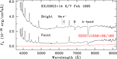
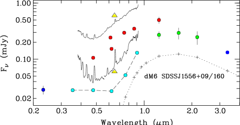
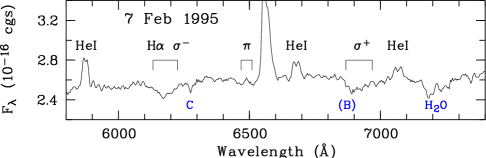
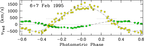
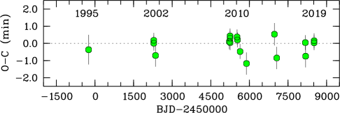
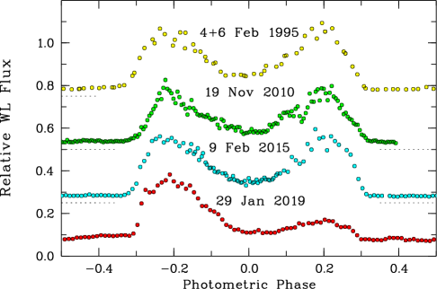
Figure 7: RX J0953.1+1458. Left, top: Combined blue and red flux-calibrated medium-resolution spectra at orbital maximum and minimum. Second from top: Zoom into a difference spectrum emphasizing the H$\alpha$ Zeeman features. Third from top: Mean radial-velocity curves of the narrow and broad emission-line components of H$\alpha$. Bottom: $O-C$ diagram for the center of the bright phase of the optical light curves. Right, top: Overall spectral energy distribution, involving nonsimultaneous data (see text). Center: Optical light curves taken in WL, taken in 1995, 2010, 2015, and 2019, shifted by multiples of 0.25 units in the ordinate. Bottom: PSPC X-ray light curve taken in the RASS. The photometric phase is from Eq. 7.

7 RX J0953.1+1458 (= J0953) in Leo

J0953 was discovered in the RASS as a soft X-ray source, spectroscopically identified by us as a polar, and is listed as such in Beuermann & Burwitz (1995) and Beuermann et al. (1999). The system shows comparatively weak He ii$\lambda$4686 line emission and was reclassified by Oliveira et al. (2020) as an intermediate polar. We do not share their interpretation and confirm J0953 as a synchronized polar.

7.1 X-ray observations

In the RASS, the star was detected in November 1990 with a mean PSPC count rate of $0.24\,\pm\!0.03$ cts s^-1 and a hardness ratio $HR1\!=\!-0.72\!\pm\!0.07$ (Table 1). The RASS light curve (Boller et al., 2016) in Fig. 7, lower right-hand panel, revealed a well-defined bright phase with a mean count rate of $0.43\!\pm\!0.03$ cts s^-1. The phase convention refers to the center of the optical bright phase (Eq. 7). Because the flux goes to zero during the faint phase, the orbital mean RASS spectrum is readily scaled upward to that of the bright phase. The extinction in front of the source is $E_{\mathrm{B-V}}$$\,=\!0.024\!\pm\!0.006$ (Lallement et al., 2018) and corresponds to $N_{\mathrm{H}}$$\,=\!(2.2\!\pm\!0.6)\,\times\,10^{20}$ H-atoms cm^-2 (Nguyen et al., 2018). When this value is adopted, the spectral fit with the model of Sect. 3.1 yields the bolometric X-ray fluxes and luminosities listed in Table 2. In spite of the rather low equivalent width of He ii$\lambda$4686 (Table 5), this appears to be the high state of J0953.

7.2 Orbital period and ephemeris

The orbital period of J0953 was measured on 4–6 February 1995 by phase-resolved $V$-band photometry with the ESO-Dutch 90 cm telescope that extended over four consecutive orbital periods. Photometry was performed relative to SDSS J095309.26+150118.8, which is located 15″ E and 162″ N of the target and has AB magnitudes $g\!=\!16.19$, $r\!=\!15.55$, and $i\!=\!15.33$. J0953 was observed in WL by Kanbach et al. (2008) in 2002 and repeatedly by us between 1995 and 2019 (Table 4). The light curves of J0953 (Fig. 3 and 7) are good examples of a single-pole accretor with strong cyclotron beaming. In search of an appropriate fiducial mark for the period measurement, we opted for the center of the bright phase, calculated as the mean of the ingress and egress times. A linear fit to 18 center-bright times yielded the alias-free ephemeris

$$T_{\mathrm{cb}}\!=\!\mathrm{BJD(TDB)}\leavevmode\nobreak\ 2455217.96104(8)+0.072022401(3)\,E.$$ (7)

The bottom left panel of Fig. 7 shows the O-C diagram. All measured times are listed in Table 12 in Appendix C.

7.3 Trailed spectrophotometry and Zeeman spectroscopy

We obtained trailed optical spectra of J0953 on 5–8 February 1995, using the same setup as for the previous target (Table 3). In this case, the correction for the Meinel OH-bands was less problematic. We show the mean faint-phase spectrum and the mean spectrum for intervals around the orbital maxima in Fig. 7, top left panel. The system reached $r\!\simeq\!16.7$ at orbital maximum, dropping to $19.5$ in the faint phase. The secondary is detectable in the observed faint-phase spectrum. Its spectral type cannot securely be determined, but at the orbital period of J0953, the evolutionary sequence of Knigge et al. (2011) predicts a secondary star of spectral type about dM5.5. We adopted the dM6 (or dM5.5) star SDSS J155653.99+093656.5 with $i\!=\!15.12$ as template and show its spectrum, adjusted by a factor of $160\,\pm\,30$, in the upper left panel (red curve). This factor yields the $i$-band magnitude and flux of the secondary star as $20.63\!\pm\!0.21$ and $0.0203\!\pm\!0.0038$ mJy, respectively.

The red bright-phase continuum plausibly represents cyclotron emission from the primary pole; it extends to about 5000 Å (12th harmonic), where the blue stream emission overtakes. The bright-phase spectrum contains Zeeman features of H$\alpha$, seen more clearly in the difference spectrum of bright and faint phases (second left-hand panel from the top). The H$\alpha$ $\pi$ and $\sigma^{-}$ components are undisturbed, while the $\sigma^{+}$ component coincides with the uncorrected atmospheric B band. These rather sharp lines with the resolved $\pi$-components are of nonphotospheric origin and of a type usually referred to as halo lines (Ferrario et al., 2015, their Table 2). They occur in cool matter in the vicinity of the hot plasma emitting the cyclotron radiation. In V834 Cen, this is the free-falling pre-shock matter (Schwope & Beuermann, 1990), and in BL Hyi more stationary matter at an uncertain location (Schwope et al., 1995). In both cases the observed lines indicate the field strength in the vicinity of the accretion region. With 19 MG, the derived field strength in J0953  is rather low for a polar.

We measured the radial velocities of the narrow and broad components of the Balmer lines and show the results for H$\alpha$ in the third left-hand panel of Fig. 7. The narrow component has a velocity amplitude $K_{2}^{\prime}\!=\!254\!\pm\!7$ km s^-1 and a blue-to-red zero crossing at photometric phase $\phi_{\mathrm{br}}\!=\!0.11\,\pm\,0.01$, defining spectroscopic phase as $\phi_{\mathrm{sp}}\!=\!\phi_{\mathrm{ph}}-0.11$, which is bona fide also the true binary phase. The broad component has a somewhat uncertain $K_{\mathrm{broad}}\,\sim\,920$ km s^-1 with $\gamma_{\mathrm{broad}}\!\sim\!400$ km s^-1. It reaches maximum positive radial velocity at photometric phase $\phi_{\mathrm{ph}}\!=\!0.02\,\pm\,0.02$, almost coincident with the closest approach to the accretion funnel, when the BBC is moving away from the observer.

The question of a possible asynchronism was raised by Oliveira et al. (2020), who considered J0953 as an intermediate polar. Their argument was based on a single double-peaked spectrum, which they interpreted as originating from an accretion disk. The gray plot in Fig. 2 shows that J0953 may display a double-peaked line profile near $\phi_{\mathrm{sp}}\!=\!0.5$ that originates, however, from the superposition of NEL and the broad component, notably in form of the HVC. We measured the spectroscopic period by combining the data of 6 and 7 February 1995, and obtained $P_{\mathrm{n}}\!=\!0\,\aas@@fstack{d}07188(15)$ and $P_{\mathrm{b}}\!=\!0\,\aas@@fstack{d}07204(9)$ for the narrow and broad component, respectively. Both periods agree within the errors with the photometric period of Eq. 7 and limit any asynchronism to a level of $2\,\times\!10^{-3}$. Because the simple light curve did not change over more than 20 years, however, this places the limit at lower than $10^{-5}$.

7.4 Spectral energy distribution

The overall SED is shown in the upper right panel of Fig. 7. The observed spectra at orbital maximum and minium (black curves) and the MONET fluxes (yellow triangles) delineate the range of the orbital and temporal variability over the years. The Gaia, Pan-STARS, and a 2MASS $J$-band point (red dots) fall within this range. The GALEX point (blue), the SDSS photometry (cyan), part of the 2MASS data (green), and the WISE W1 point (blue) belong to a low or an intermediate state.

The SED of the adjusted dM6 secondary star is shown by the dashed curve. An earlier star, adjusted to the same $i$-band flux, would have lower IR fluxes. The secondary accounts for part of the red and IR flux observed in the SDSS (cyan), the 2MASS (green) and WISE (blue). The remaining flux in the IR represents cyclotron radiation or stream emission. The low fluxes measured in the SDSS (cyan) and with GALEX (blue) can be accounted for by a WD of 0.75 $M_{\odot}$ with radius $7.6\,\times\!10^{8}$ cm and effective temperature 12000 K, placed at the Gaia distance of 448 pc (blue curve). Measuring the temperature and radius of the WD spectroscopically should be feasible.

7.5 System parameters

At the orbital period of J0953, the evolutionary model of Knigge et al. (2011) predicts a moderately bloated secondary star with a mass of 0.118 $M_{\odot}$, radius of 0.161 $R_{\odot}$, and a spectral type dM5.5 with an $i$-band surface brightness $S_{\mathrm{i}}\!\simeq\!8.4$. The predicted $i$-band magnitude and flux at the Gaia distance are 20.62 and 0.0205 mJy, respectively, in agreement with the observed quantities (Sect. 7.3). For further analysis, we converted the radial-velocity amplitude $K_{2}^{\prime}\!=\!254$ km s^-1 into $K_{2}$ with our irradiation model BR08. The well-defined length of the self-eclipse, $\Delta\phi\!\simeq\!0.40$, places the accretion region in the upper hemisphere of the WD. The deep cyclotron minimum and the lack of an absorption dip require $i\,\la\,\beta\!\simeq\!\zeta$ (Sect. 3.5). Eq. 3 gives $i\!\simeq\!55\!-\!60$° and the measured value of $K_{2}^{\prime}$ gives $M_{1}\!\simeq\!0.58\,-\,0.68$ $M_{\odot}$. The standard primary mass of Knigge et al. (2011) of 0.75 $M_{\odot}$ would require an inclination of 50°.

The accretion rate derived from the X-ray luminosity is $\dot{M}_{\mathrm{x}}\!=\!4.6\!\times\!10^{-11}$ $M_{\odot}$yr^-1. The estimate of the cyclotron luminosity in Table 2 is based on the observed optical spectrophotometry, extrapolated into the near-IR. When it is included, the required accretion rate rises to $\dot{M}_{\mathrm{x+cyc}}\!=\!5.8\!\times\!10^{-11}$ $M_{\odot}$yr^-1 for a WD of 0.63$M_{\odot}$. The corresponding equilibrium temperature of the compressionally heated WD would be 10400 K. The predicted 4600Å flux of the WD of 0.027 mJy agrees closely with the dereddened SDSS photometric g-band flux of $0.026\!\pm\!0.02$ mJy (Fig. 7, upper right panel, cyan dots). The SDSS $ugr$ points and the GALEX flux with $0.033\!\pm\!0.03$ mJy (blue dot) define a flat spectrum, which likely represents the magnetic WD. The agreement between predicted and observed spectral fluxes suggests that the current effective temperature of the WD in J0953 and its equilibrium temperature do not differ substantially.

8 RX J1002.2–1925 (= J1002) in Hydra

J1002 was discovered in the RASS as the brightest and softest X-ray source in our sample, spectroscopically identified by us as a polar, and it is listed as such in Beuermann & Thomas (1993), Beuermann & Burwitz (1995), and Thomas et al. (1998). Despite its high degree of variability, it seems to be a tightly synchronized polar.

8.1 X-ray observations

J1002 was detected in the RASS with a mean count rate of $0.69\!\pm\!0.04$ cts s^-1 and a hardness ratio $HR1\!=\!-0.97\!\pm\!0.03$, implying that 98% of the photons had energies below the carbon edge at 0.28 keV (Table 2). J1002 was reobserved with ROSAT and the PSPC in 1992 and 1993 and with the HRI in 1995. In 1992, it was in a low state, with $-0.0002\pm 0.0024$ PSPC cts s^-1, and in 1993 again in a high state, with 0.71 PSPC cts s^-1 and 97% soft photons. Ramsay & Cropper (2003) observed it with XMM-Newton in 2001 in an intermediate state. We reanalyzed their observation for the present purpose. The lower left-hand panels of Fig. 8 show the orbital light curves of the RASS PSPC, the 1995 ROSAT HRI, and the 2001 XMM-Newton EPIC pn and MOS12 observations placed on the ephemeris of Eq. 8. Common properties are a bright phase that lasts for $\sim\!$75% of the orbital period and a narrow absorption dip near its center. This repetitive feature marks the instance when the line of sight to the WD passes through the magnetically guided part of the accretion stream.

Table 6: Fit parameters for the XMM-Newton pn and the ROSAT PSPC bright-phase X-ray spectra of J1002. The letter “f” denotes a frozen parameter. The quantity $f_{\mathrm{sx,bol}}\,=\!c_{\mathrm{sx}}f_{\mathrm{bb1,bol}}$ with $c_{\mathrm{sx}}\,=\!3$ and $f_{\mathrm{bb1,bol}}$ the bolometric flux of the single-blackbody fit.

Fit	Detector	$N_{\mathrm{H}}$	$N_{\mathrm{H,int}}$	$f_{\mathrm{pc}}$	k$T_{\mathrm{bb1}}$	$f_{\mathrm{sx,bol}}$	$f_{\mathrm{th,bol}}$	$\chi^{2}$ (dof)
		($10^{21}$ cm-2)			(eV)	($10^{-11}$erg/cm2s)
1	pn	2.15			38.1	2.05	0.11	81.9  (56)
2	pn	0.01	544	0.69	53.8	0.53	0.26	45.6  (53)
3	pn	1.00 f	536	0.69	50.1	0.86	0.27	46.4  (53)
4	pn	2.90 f	520	0.69	43.2	2.34	0.29	49.1  (54)
5	PSPC	1.00 f	100 f	1.0 f	50.0	1.78	0.22	33.7  (39)

The XMM-Newton EPIC pn observation and the 1993 ROSAT PSPC observation both cover exclusively the bright phase. The PSPC spectrum is not shown. A graph of the EPIC pn spectrum can be found in Fig. 7 of Ramsay & Cropper (2003). We fit both spectra with the model of Sect. 3.1. Table 6 summarizes the results. The model in line 1 is a moderately successful fit to the pn spectrum with $N_{\mathrm{H,int}}$$\,=\!0$. With the model in line 2, we confirm the findings of Ramsay & Cropper (2003) that the fit (i) prefers an interstellar column density close to zero and (ii) benefits from the inclusion of an internal absorber. A very low value of $N_{\mathrm{H}}$ is unrealistic, however, given the Gaia distance of 797 pc. The total galactic column density at the position of J1002 is $N_{\mathrm{H,gal}}\!=\!3.96\,\times\!10^{20}$ H-atoms cm^-2 (HI4PI Collaboration et al., 2016) and the total extinction is $E_{\mathrm{B-V}}$$\,=\!0.0351$. A sizeable fraction seems to arise in front of J1002, $E_{\mathrm{B-V}}$$\,\simeq\!0.031\!\pm\!0.009$ (Lallement et al., 2018) or $N_{\mathrm{H}}$$\,=\!(2.9\,\pm\,0.9)\!\times\!10^{20}$ H-atoms cm^-2 (Nguyen et al., 2018). Because of tradeoffs between the parameters $N_{\mathrm{H}}$ and k$T_{\mathrm{bb1}}$, reasonably good fits are obtained for any column density up to $N_{\mathrm{H,gal}}$ (lines 2 to 4). Fitting the 1993 PSPC and the 2001 pn spectrum with the same $N_{\mathrm{H}}$–k$T_{\mathrm{bb1}}$ combination requires $N_{\mathrm{H}}$$\,=\!1.0\,\times\!10^{20}$ H-atoms cm^-2 and k$T_{\mathrm{bb1}}$$\,=\!50$ eV (lines 3 and 5). The blackbody fluxes for the two observations differ by about a factor of two, which is a measure of the different brightness levels during the two runs. We adopted these fits, but consider the fluxes of lines 3 and 5 in Table 6 as approximate lower limits and marked them as such in Table 2.

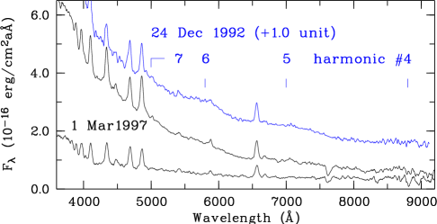
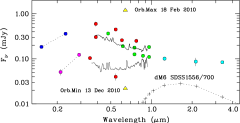
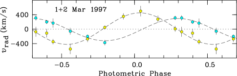
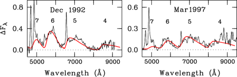
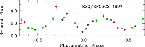
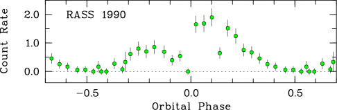
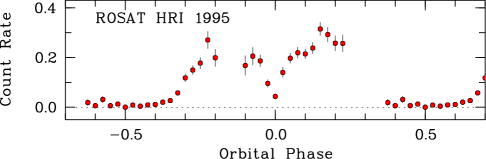
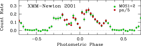
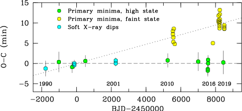
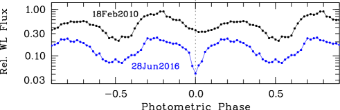
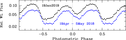
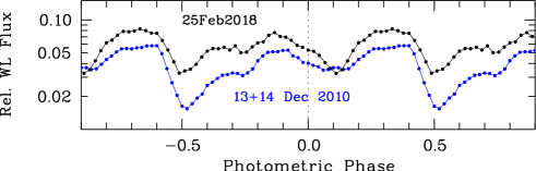
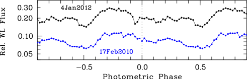
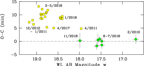
Figure 8: RX J1002.2–1925. Left, top: Flux-calibrated low-resolution spectra on 24 December 1992 and at orbital maximum and minimum on 1 March 1997. Cyclotron harmonics are indicated. Left, second from top: Balmer-line radial velocities of the narrow and broad components from spectra of 1 and 2 March 1997. Left, third from top: Spectral flux in the $B$ band of 1 and 2 March 1997 in units is $10^{-16}$ ergs cm^-2s^-1Å^-1. Left, next three panels: Soft X-ray light curves of 1990, 1995, and 2001. Right, top: Overall nonsimultaneous SED. Right, second from top: Cyclotron spectra on 24 December 1992 and 1 March 1997 with models for a field strength of 33 MG. Right, next four panels: Samples of optical light curves taken in WL, illustrating the variability of primary and secondary minima. Left, bottom: $O-C$ diagram for the primary minimum, from light curves with peak orbital WL AB magnitude $w\!\la\!18$. Right, bottom: $O\!-\!C$ for the primary minimum vs. $w$.   The photometric phase is from Eq. 8.

8.2 Orbital ephemeris

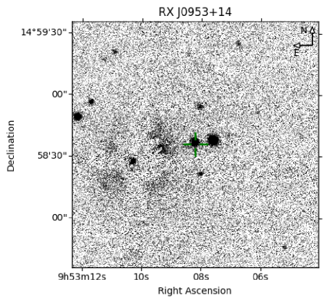
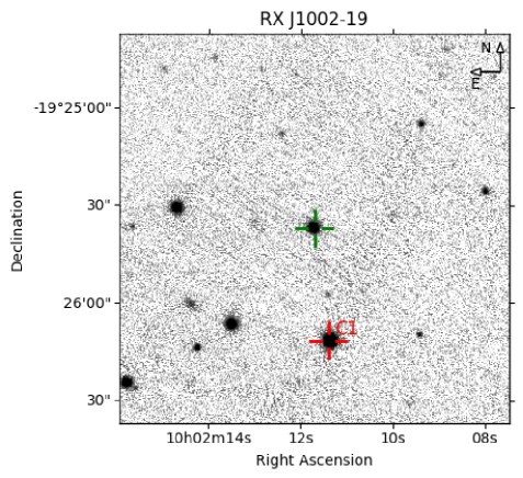
Figure 11: Left: Finding chart for RX J0953.1+1458. Size is 2′$\times$2′. The comparison star is 9″ W and 101″ S of the target and outside the image. Right: Finding chart for RX J1002.2–1925. Size is 2′$\times$2′. The comparison star is 5″ W and 36″ S of the target and marked C1.

The RASS observation has suggested a periodicity with $P_{\mathrm{orb}}\!=\!0\,\aas@@fstack{d}0697(4)$, which was refined by the separation of the narrow soft X-ray absorption dips in the 1995 HRI observation to $P_{\mathrm{orb}}\!=\!0\,\aas@@fstack{d}0694(2)$. The five X-ray dips, one in the RASS, two in the ROSAT HRI, and two in the XMM-Newton observation (pn and MOS), did not suffice for an alias-free ephemeris, however. Phase-resolved optical photometry and spectrophotometry of J1002 was performed in 1992, 1995, and 1997. We added WL photometry with the MONET telescopes in 27 nights between 2010 and 2019 (Tables 3, 4, and 13). In the photometric runs, the brightness of the target was measured relative to a comparison star C1 located at RA(2000) = $10^{\mathrm{h}}02^{\mathrm{m}}11\aas@@fstack{s}4$, DEC(2000) = $-19\degr 26\arcmin 12\arcsec$ or 5″ W and 35″ S of the target (Fig 11). It has an AB magnitude $r\!=\!15.95$  and colors $g-r\!=\!0.66$ and $r-i\!=\!0.24$, giving $w\!\simeq\!16.0$ for unity relative to the WL flux.

Improving the X-ray derived period by optical data proved tedious because the light curves show a pronounced variability, display phase shifts in the positions of the minima, and possess two minima per orbit, which annoyingly flipped the role of the more prominent one over the years. The spectrophotometric light curve of 1997 in the left part of Fig. 8 (third panel from the top) and selected WL light curves of 2010–2019 on the right side (panels three to six from the top) provide an overview. All light curves are phased on the ephemeris of Eq. 8 used as a common reference. They show that (i) the cyclotron-dominated bright phase and the X-ray bright phase coincide, (ii) the primary optical minimum at $\phi\!\simeq\!0$ is produced by cyclotron beaming and occurs close in time to the X-ray absorption dip (see the discussion in Sect. 3.5), and (iii) the secondary minimum occurs when the accretion spot dips behind the horizon at $\phi\!\simeq\!0.5$. The light curves in the right-hand panels are highly variable. The cases of 18 February 2010 and 28 June 2016 suggest that either the primary spot wanders in latitude or the minimum is filled up by the emission of an independent second accretion region. Repeatedly over the years, we observed light curves in which the separation of the primary and the secondary minimum differed from half an orbital period (e.g., 13+14 December 2010 and 25 February 2018). This apparent shift is probably caused by a second emission region that appears near $\phi\!=\!0.6$ (compare the similar blue model light curve in the right panel of Fig. 3). On other occasions, both minima appear displaced by up to +0.12 in phase, requiring a longitudinal shift of the spot by up to 40°(e.g., April–May 2018). The light curves of 4 January 2012 and 17 February 2010 lack any trace of the primary minimum.

Our search for a long-term ephemeris is based on a total of five X-ray dips and 70 times of optical minima, not all measured from complete orbital light curves. Because there is no unique way to distinguish primary and secondary minima observationally, we started our search for a long-term ephemeris by considering the mixed bag of primary and secondary minima and calculating a periodogram in the vicinity of $P_{\mathrm{orb}}$/2. This procedure yielded a unique (alias-free) ephemeris. We assigned cycle number $E\!=\!0$ to the X-ray dip in the XMM-Newton pn light curve as our key primary minimum. This allowed us to identify all minima with even cycle numbers on the $P_{\mathrm{orb}}$$/2$ fit as primary ones. We proceeded by calculating an ephemeris on a $P_{\mathrm{orb}}$ basis for the subset of all primary minima with redefined cycle numbers. We kept the definition of $E\!=\!0$.

We show the $O\!-\!C$ values of all primary minima based on the ephemeris of Eq. 8 in the bottom left panel of Fig. 8. This ephemeris satisfies all minima of 1990–2001 and also selected minima of 2010, 2014, 2016, and 2018 (green dots, shown with error bars), but fails to meet other groups of minima of 2010, 2017, 2018, and 2019 (yellow dots, shown without error bars to avoid clutter). The likely physical cause of the discrepant $O\!-\!C$ values becomes clear from the bottom right panel, where we show the same data plotted versus the brightness of the system, measured by the peak orbital WL magnitude $w$. In high states with $w\!<\!18$, $O\!-\!C$ averages zero, while in intermediate or low states with $w\!\ga\!18$, $O\!-\!C$ reaches up to $\sim\!12$ min. Obviously, no linear ephemeris can describe the up and down of $O\!-\!C$.

Selecting the early data (five X-ray dips and four primary optical minima) and the seven primary minima from high-state light curves with $w\!<\!18$ defines the alias-free ephemeris

$$T_{\mathrm{min}}\!=\!\mathrm{BJD(TDB)}\leavevmode\nobreak\ 2452254.38167(21)+0.069427553(5)\,E,\leavevmode\nobreak\ \leavevmode\nobreak\ \leavevmode\nobreak\$$ (8)

which served as our reference and is represented by the dashed line in the bottom left panel of Fig. 8. The X-ray data represent high states (ROSAT) or a moderately high state (XMM-Newton). The spectrophotometry of 1992 and 1997 is characterized by strong He ii$\lambda$4686 emission lines (Table 5), which indicates the presence of an intense XUV component and marks them as ’high state’ as well. Fitting the early data alone yields the same ephemeris as Eq. 8 within the uncertainties. This shows that the early X-ray and optical data and the later high-state data are entirely compatible with a common linear ephemeris.

Selecting instead the mutually exclusive subset of primary minima of 2010–2019 with $w\!>\!18$ (yellow dots in the bottom panels of Fig. 8), supplemented by the seven timings of 1990–1997, but excluding the now discrepant 2001 XMM timings, we obtain the longest period compatible with part of the data,

$$T_{\mathrm{min}}\!=\!\mathrm{BJD(TDB)}\leavevmode\nobreak\ 2452254.38353(25)+0.069427610(4)\,E.\leavevmode\nobreak\ \leavevmode\nobreak\ \leavevmode\nobreak\$$ (9)

This ephemeris has an orbital period 4.9 ms longer than that of Eq. 8 and is represented by the dotted line in the bottom left panel of Fig. 8. Both ephemerides assign the same cycle numbers to all minima of the 30 yr covered by our data. Despite the remaining uncertainty, our ephemerides are therefore alias-free. The times of all primary minima used for Eq. 8 or Eq. 9 are listed in Table 13 in Appendix C. The high-state spot position is stable over at least about 1.5 mag in $w,$ and we argue that the period in Eq. 8 more likely represents the true binary period.

The $O\!-\!C$ variations in J1002 are unlike anything observed in synchronized polars. Does J1002 lack synchronism? It showed no evidence for a shorter, intermediate-polar like periodicity. Between 1990 and 2001, X-ray period, optical photometric period, and spectroscopic period agreed, severely limiting the permitted degree of asynchronism. The data of 26 December 1992 to 1 January 1993 and of $1\!-\!2$ March 1997 yielded spectroscopic periods of 0 $\aas@@fstack{d}$069400(50) and 0 $\aas@@fstack{d}$069422(110), which deviate from the photometric period of Eq. 8 by $-2.4\,\pm\,4.3$ s and $-0.5\,\pm\,9.5$ s, respectively. The two epochs combined lead to a spectroscopic period of 0 $\aas@@fstack{d}$06942755(19), which perfectly agrees with the photometric period within its error of 17 ms. This excludes a sizeable asynchronism as in the post-nova V1500 Cyg, but not necessarily the minute level detected in DP Leo and thought to reflect the slow oscillation of the two stellar components about their magnetostatic equilibrium position (Beuermann et al., 2014). However, even if active in J1002, this process provides no explanation for the observed up and down of $O\!-\!C$. We are therefore left with the classical explanations: (i) At a reduced accretion rate, the stream penetrates less deeply into the magnetosphere, the spot moves closer to the line connecting the two stars, and the closest approach to the spot occurs later. (ii) At a reduced accretion rate, the stream switches from a ballistic trajectory in the orbital plane to a magnetically guided path starting from the secondary star, a possibility considered in Papers I and II. (iii) In a complex field geometry, the stream may be directed to different positions on the WD surface depending on the accretion rate and the ram pressure it exerts. All polars experience drastic variations in the accretion rate, yet none has so far displayed apparent or real spot movements similar to those observed in J1002.

8.3 Spectrophotometry and cyclotron spectroscopy

Low- and medium-resolution phase-resolved spectrophotometry was performed in December 1992 and March 1997 (Table 3). The top left panel in Fig. 8 shows the single spectrum of 1992 (blue) and the 1997 spectra at orbital maximum and minimum (black). They are characterized by a blue continuum, strong Balmer and He ii$\lambda$4686 emission lines, the Balmer jump in emission, and the absence of spectral features of the stellar components. The equivalent widths of He ii$\lambda$4686 and H$\beta$ (Table 5) fall in the general area populated by polars (Oliveira et al., 2020, their Fig. 2). Furthermore, the bright-phase line ratio near unity indicates that J1002 was in a high state in December 1992 and March 1997. The Balmer lines in the medium-resolution spectra of both years are fairly wide, as noted already by Oliveira et al. (2017). Their FWHM varies between 1100 and 2300 km s^-1 over the orbit. Balmer and helium lines consist of a broad component, representing a mixture of the BBC and HVC, and a well-defined narrow component, representing the NEL. The second left panel in Fig. 8 shows the radial-velocity curves of the narrow component, measured from the 2 March 1997 spectra, and of the broad component, obtained from 1 and 2 March. The narrow component has a radial-velocity amplitude $K_{2}^{\prime}\!=\!307\pm 30$ km s^-1, with a blue-to-red zero crossing at photometric phase $\phi_{\mathrm{br,n}}\!=\!0.055\!\pm\!0.024$. The broad component has a radial-velocity amplitude $K_{\mathrm{broad}}\!=\!436\pm 47$ km s^-1, reaching maximum positive radial velocity at $\phi_{\mathrm{broad}}\!=\!0.044\!\pm\!0.013$. If the narrow line tracks the motion of the secondary star, spectroscopic (or binary) and photometric phases are related by $\phi_{\mathrm{sp}}\!=\!\phi_{\mathrm{ph}}-0.055$, with $\phi_{\mathrm{ph}}\!=\!0$ some $20\degr\pm\,9\degr$ in azimuth before inferior conjunction. Maximum positive broad-line radial velocity occurs $4\degr\!\pm\!5\degr$ before inferior conjunction, but primary minima that are 10 min late occur at binary phase $\phi_{\mathrm{sp}}\!\simeq\!0.05$ or 5 min past inferior conjunction. Very similar numbers were obtained for 1992. Whether they still applied between 2010 and 2019, when the pronounced $O\!-\!C$ variations occurred, remains uncertain.

The spectrum of 24 December 1992 displays weak cyclotron lines superposed on the blue optically thick cyclotron continuum and the optically thin stream emission. Lines at the same positions are also detected in the difference between the 1997 orbital maximum and minimum spectra. They are displayed in Fig. 8 (second right-hand panels from the top) with an estimated continuum interactively subtracted. They were fit by constant-temperature models calculated with the theory of Chanmugam & Dulk (1981) (red curves) for a field strength of 33 MG with k$T_{\mathrm{e}}\!\simeq\!7\,$ keV, an angle against the field line $\theta\!=\!70-80^{\circ}$, and a thickness parameter log $\Lambda\!\simeq\!3.8$. For these parameters, the lines represent the fourth to seventh harmonic. We cannot entirely exclude that the observed lines are harmonics 3 – 6 in a field of 40 MG.

8.4 Spectral energy distribution

The top right-hand panel of Fig. 8 shows the overall SED of J1002 that includes the 1 March 1997 bright and faint-phase spectra (black solid curves), a summary of nonsimultaneous photometry, and a representation of the secondary star from our dynamical model presented below. The photometry is from GALEX (blue), the XMM-Newton UV monitor (magenta), Gaia, SkyMapper, and the XMM-Newton V monitor (red), PanSTARRS (green), VISTA (cyan), and ALLWISE W1 (magenta). The full range of the brightness variations of our extensive MONET WL observations (yellow triangles) spans a factor of 50. None of the observations represents a low state, although such drops in brightness exist, as evidenced by the 1992 ROSAT PSPC observation and the long-term light curve of the Catalina Sky Survey (Drake et al., 2009), which shows a drop to $>\!20$ mag at the end of 2007 from a general level of $18\pm 1$ mag.

8.5 System parameters

At the orbital period of J1002, the evolutionary model of Knigge et al. (2011) predicts a mildly bloated secondary star with a mass of 0.108 $M_{\odot}$, a radius of 0.153 $R_{\odot}$, and a spectral type dM5.6. With an $i$-band surface brightness $S_{\mathrm{i}}\!\simeq\!8.5$, the $i$-band magnitude and flux at the Gaia distance are 22.08 and 0.0053 mJy. It is not surprising that the secondary star is not detected in the observed spectrum. The occurrence of the soft X-ray absorption dip requires that the inclination $i$ of the system exceeds the inclination of the accreting field line $\zeta$ in the accretion spot. In the optical and X-ray light curves, the primary accretion spot is visible for 3/4 of the orbital period. It is self-occulted for a phase interval $\Delta\phi\!\simeq\!0.25$, implying $i\!>\!50$° (Eq. 3 in Sect. 3.5). On the other hand, if the deep minima in some light curves are produced by cyclotron beaming, $i$ cannot be too large, suggesting $i\!\simeq\!55-60$°. When we convert the observed NEL radial-velocity amplitude of $K_{2}^{\prime}\!=\!307$ km s^-1 into $K_{2}$ with our irradiation model BR08, the corresponding mass range is $M_{1}\!\simeq\!0.75\,-\,0.89$ $M_{\odot}$. For $i\!=\!75$°, just avoiding an eclipse, the minimum primary mass consistent with the measured $K_{2}^{\prime}$ is $M_{1}\!\simeq\!0.63$.

The accretion rate based on the 1993 high-state PSPC observation is $\dot{M}_{\mathrm{x}}\!\ga\!6.3\,\times\!10^{-11}$ $M_{\odot}$yr^-1. When the cyclotron flux from the high photometric data points in the SED of Fig. 5 (see Table 2 column 13) is included, the required accretion rate rises to $\dot{M}_{\mathrm{x+cyc}}\!\ga\!8.7\,\times\!10^{-11}$ $M_{\odot}$yr^-1. Both $\dot{M}$ values are quoted as lower limits because they are based on an X-ray fit with a lower-than-standard interstellar absorbing column density (Sect. 8.1). Correspondingly, for the XMM-Newton observation in a moderately high or intermediate state complemented by an estimate of the cyclotron luminosity from the orbital mean of our spectrophotometry, $\dot{M}_{\mathrm{x+cyc}}\!\ga\!4.7\,\times\!10^{-11}$ $M_{\odot}$yr^-1. If either one of these rates equals the secular mean, the corresponding equilibrium temperatures of the WD from compressional heating would fall between $\ga\!12800$ K and $\ga\!15000$ K for a WD of 0.82 $M_{\odot}$. The predicted 4600Å flux of the WD in the high state is 0.014 mJy, about a factor of two below the lowest MONET flux (yellow triangle). A spectroscopic temperature measurement and mass estimate of the WD in a low state appears feasible.

9 Discussion

In this last paper of a series of three, we report results on five ROSAT-discovered polars collected over three decades. Papers I and II (Beuermann et al., 2017, 2020) contained in-depth analyses of V358 Aqr and the eclipsing polar HY Eri. The results on the present five objects are less complete, but they are accompanied by accurate linear ephemerides, which allow the correct phasing of past and future observations. There is no evidence of a variation in orbital period or for an asynchronism in any of the five targets, and we consider them as bona fide synchronous rotators.

Two of our targets, J0154 and J0859, belong to the league of bright polars that reach 15 or 16 mag. At the other end of the brightness scale, the distant object J0600 resides near the bounce period and does not appear to exceed 19 mag. J0154 is the second polar after VY For (Beuermann et al., 1989), in which the main active pole appears to be permanently hidden behind the WD. Cropper (1997) advocated polarimetry of VY For to investigate its accretion geometry. Studying the brighter system J0154 may be more profitable.

The evolution of polars differs from that of nonmagnetic CVs. The concept of reduced magnetic braking of Li et al. (1994) was devised to explain the effective disappearance of the period gap for polars and was successfully employed by Belloni et al. (2020) in their binary stellar evolution code. Polars show at most a remnant gap, and systems with $P_{\mathrm{orb}}$$\,\la\!150$ min behave effectively as short-period polars (Schwope et al., 2020). In the current sample, this applies to J0859. There is agreement that all short period CVs suffer larger angular momentum losses (AML) than predicted by gravitational radiation alone. Knigge et al. (2011) included the additional AML as a numerical scaling factor, while Belloni et al. (2020) implemented the empirical consequential angular momentum loss eCAML of Schreiber et al. (2016) in their code. CAML describes an accretion-related process, for instance, the time-averaged Bondi-Hoyle-type frictional energy loss that the secondary star experiences in the nova shells that are expelled at intervals by the WD. Both authors effectively raised the AML and thereby $\dot{M}$ in an attempt to better match observed quantities as the bounce period or the space density of CVs.

The concept of an ’observed’ accretion rate was considered questionable for a long time, but was placed on firmer ground by (i) the advent of the Gaia trigonometric distances (Bailer-Jones et al., 2018) and (ii) the progress in constructing a 3D extinction map for the solar neighborhood (Lallement et al., 2018), which helps to derive reliable optical and X-ray luminosities. Calculating the accretion rate requires knowledge of the WD mass. For three of our targets, we measured the radial-velocity amplitude $K_{2}^{\prime}$ of the narrow component of the Balmer lines, which is thought to originate on the irradiated surface of the secondary star. Converting $K_{2}^{\prime}$ into the amplitude $K_{2}$ of the center of mass of the secondary star requires knowledge of the inclination $i$ of the system and an irradiation model for the emission line in question. In this pilot study, we have applied our irradiation model BR08 (Beuermann & Reinsch, 2008; Beuermann et al., 2017) although it was not optimized for the Balmer lines and He ii$\lambda$4686. Ways to improve $i$ have been noted in the relevant subsections. The derived primary masses depend only weakly on $M_{2}$ because the stellar models and the moderate bloating in short-period polars leave little freedom. All five systems, however, are open for a more direct determination of $M_{1}$ by a spectroscopic measurement of the temperature and radius of the WD in a low state of the respective system.

For five of the seven targets in Papers I-III of this series, we measured the field strength in the accretion region spectroscopically. The mean field strength for the present sample of 30 MG does not differ much from the 33.4 MG of the complete sample of our 27 ROSAT soft and hard X-ray discovered polars and the 38 MG of all polars in Table 2 of Ferrario et al. (2015). Measuring the WD temperature and thereby its radius requires models of magnetic atmospheres. Such models were calculated by Jordan (1992), but significant uncertainties related to Stark broadening in the presence of a magnetic field remain and we emphasize again the need for calculations of the shifts of individual Stark components (see Paper II).

The polars discussed in this paper feature X-ray spectra that consist of a soft quasi-blackbody and a hard thermal X-ray component. Hard X-rays originate primarily in the cooling flow of the accretion stream that develops downstream of the strong shock that is set up above the stellar surface. Its temperature distribution is determined by the competition between bremsstrahlung and cyclotron cooling and the associated radiative transfer (Woelk & Beuermann, 1996; Fischer & Beuermann, 2001). Soft X-rays originate from the heated stellar atmosphere of the spot and its surroundings. Insight into the temperature distribution of the optically thick soft X-ray emission was obtained from the high-resolution spectrum of the prototype polar AM Her measured down to 92 eV (135 Å) with the Low Energy Transmission Grating Spectrometer (LETGS) on board Chandra (Beuermann et al., 2012). The analysis revealed the expected spread in temperature and demonstrated that modeling the soft X-ray component by a single blackbody is a severe approximation. In the case of AM Her, the single-blackbody model underestimated the bolometric flux of the XUV and soft X-ray component by a factor of $3.7\!\pm\!0.7$. We approximately accounted for this effect by raising the bolometric energy flux obtained for a single-blackbody fit by a factor $c_{\mathrm{sx}}\!=\!3$.

Townsley & Gänsicke (2009) and Pala et al. (2020) reported reliable effective temperatures of nine polars and of 42 non-mCVs with $P_{\mathrm{orb}}$$\!<\!2.1$ h. The mean temperatures and periods are $12850\!\pm\!570$ K and 103 min for the polars and $14350\!\pm\!370$ K and 92 min for the non-mCVs. According to the theory of compressional heating of the WD (Eq. 2 in Sect. 3.3), these temperatures translate into long-term mean accretion rates of $\langle\dot{M}_{\mathrm{polar}}\rangle\!=\!6.7\,\times\!10^{-11}$$M_{\odot}$yr^-1 and $\langle\dot{M}_{\mathrm{non-mCV}}\rangle\!=\!1.05\,\times\!10^{-10}$$M_{\odot}$yr^-1, respectively, assuming a WD mass of 0.75 $M_{\odot}$. The mean accretion rate of the five polars in Table 2 with a mean WD mass of 0.72 $M_{\odot}$ and a mean period of 103 min is $\langle\dot{M}_{\mathrm{x+cyc}}\rangle\!=\!6.8\,\times\!10^{-11}$$M_{\odot}$yr^-1 in their normal high states. We consider the close agreement with $\langle\dot{M}_{\mathrm{polar}}\rangle$ coincidental, but the general agreement supports our upward correction of the single-blackbody flux by the factor $c_{\mathrm{sx}}\!=\!3$. The mean temperature of single-blackbody fits for the five targets in this paper is 39 eV, which is similar to that of AM Her, k$T\mathrm{bb}\!=\!32.3$ eV. Using a common value of $c_{\mathrm{sx}}$ therefore appears plausible, but in general, employing a multitemperature model is preferable.

Different mean accretion rates for short-period polars and non-mCVs are currently not predicted by the evolutionary models. Knigge et al. (2011) do not distinguish between the subtypes of CVs. In their best-fit model, they predict $\dot{M}\!=\!7.0\,\times\!10^{-11}$$M_{\odot}$yr^-1 at 100 min for $M_{1}\!=\!0.75$ $M_{\odot}$, which corresponds rather to the temperature-derived value for polars than to that for non-mCVs. Belloni et al. (2020) explicitly accounted for the reduced magnetic braking in polars, but at short orbital periods or $M_{2}\!<\!0.20$ $M_{\odot}$, the fraction $\Phi$ of open field lines of the secondary star vanishes for a CV with $M_{1}\!=\!0.75$ $M_{\odot}$ and $B\!=\!30$ MG (Belloni et al., 2020, their Fig. 2). From that point on, their code assigns the same AML to polars and non-mCVs and predicts $\dot{M}\!\simeq\!1.0\,\times\!10^{-10}$$M_{\odot}$yr^-1 at 100 min, which is correct for non-mCVs, but exceeds $\langle\dot{M}_{\mathrm{polar}}\rangle$. Our targets with known field strengths, J0859, J0953, and J1002, lie in the $\Phi\!=\!0$ regime. Hence, there is evidence that short-period polars and non-mCVs evolve differently, but the physical cause remains elusive so far.

The question of the energy balance between the soft and hard X-ray emission of polars was intensely debated at the time when the ROSAT and XMM-Newton soft X-ray measurements became available (e.g., Ramsay et al., 1994; Beuermann & Burwitz, 1995; Ramsay & Cropper, 2004a). The background was the prediction by King & Lasota (1979) and Lamb & Masters (1979) that one-half of the accretion energy escaped as hard X-rays and the other half was intercepted by the photosphere of the WD and reprocessed into soft X-rays. The high sensitivity of ROSAT for soft X-rays and its very limited hard X-ray response led to the notion that intense soft X-ray emission was one of the hallmarks of polars, and the luminosity ratio of soft to hard X-rays seemed to exceed unity by a large factor. The theoretical description of shocks buried in the photosphere provided an understanding of the dominance of soft X-rays (Kuijpers & Pringle, 1982). The internal absorption of hard X-rays (Ramsay & Cropper, 2004a) showed that the hard X-ray flux had been severely underestimated and that cyclotron radiation needs to be included in the energy balance of the post-shock cooling flow. Furthermore, the case of AM Her showed that the soft X-ray luminosity had been underestimated as well. Taking all these caveats into account, the best estimate for AM Her is $L_{\mathrm{sx}}/(L_{\mathrm{hx}}+L_{\mathrm{cyc}})\!=\!4.3\!\pm\!2.0$ (Beuermann et al., 2012), and the consensus is that the luminosity ratio exceeds unity only in a small number of polars in their high-accretion states (Ramsay & Cropper, 2004b). The results for the present five sources in column 16 of Table 2 support this conclusion. When the high-state values are selected, the mean luminosity ratio is $L_{\mathrm{sx}}/(L_{\mathrm{hx}}+L_{\mathrm{cyc}})\!=\!2.2\!\pm\!1.1$. Furthermore, at the reduced accretion rate in intermediate and low states the temperature of the heated surrounding of the spot drops and the emission moves out of the soft X-ray band, causing the system to turn into a (apparently) hard X-ray source (Ramsay et al., 2004; Beuermann et al., 2008; Schwope et al., 2020).

We have analyzed five previously neglected polars and derived accretion rates based primarily on ROSAT PSPC data. A modern instrument such as eRosita (Predehl et al., 2020) will provide a more adequate data base for an up-to-date study of a larger population of CVs.

Appendix A ROSAT count rates and energy fluxes

The polars discussed in this paper were discovered as soft high galactic latitude X-ray sources in the ROSAT All Sky Survey (RASS). The survey was performed with the position-sensitive proportional counter (PSPC) as detector, which possesses moderate energy resolution with an FWHM of 0.4 keV at 1 keV photon energy. Subsequent pointed ROSAT observations were made with either the PSPC or the High Resolution Imager (HRI). The HRI lacked energy resolution. For quick reference, examples of an integrated PSPC count rate of 1.0 cts s^-1 converted into an HRI count rate are given in Table 7 for selected incident blackbody spectra and thermal APEC spectra absorbed by a column density $N_{\mathrm{H}}$ of neutral matter of solar composition. They were calculated with the NASA HEASARC tool PIMMS. For the blackbodies absorbed by $N_{\mathrm{H}}$$\,\la\!3\!\times\!10^{20}$ H-atoms cm^-2, the PSPC is typically more sensitive than the HRI by a factor $7\!\pm\!2$ and for the APEC spectra by about a factor of three.

In Tabel 8 we list the energy fluxes for incident blackbody spectra of three temperatures and column densities each. The first line quotes the energy flux of the absorbed spectrum incident on the detector in the ROSAT band of $0.10\!-\!2.0$ keV for 1.0 PSPC cts s^-1. The unabsorbed flux is quoted in the second and the bolometric flux in the third line. For a temperature k$T_{\mathrm{bb1}}$$\,=\!60$ eV and a low column density, the PSPC measures an energy flux that is not far from the bolometric flux. For 20 eV, however, it recovers only a small fraction of the flux and the corrections become very large.

Table 7: HRI count rates equivalent to 1 PSPC cts s^-1 for blackbody and thermal APEC spectra with the quoted temperatures and neutral absorbers $N_{\mathrm{H}}$ in erg cm^-2s^-1for 1 PSPC cts s^-1.

$N_{\mathrm{H}}$	Blackbody			APEC
(cm-2)	20 eV	40 eV	60 eV	1.0 keV	3.1 keV	9.7 keV	27.3 keV
1e19	0.112	0.127	0.143	0.319	0.242	0.270	0.271
1e20	0.117	0.138	0.162	0.362	0.315	0.310	0.313
3e20	0.129	0.163	0.203	0.392	0.360	0.352	0.352
1e21	0.147	0.280	0.379	0.407	0.385	0.375	0.373
1e22	0.494	0.350	0.377	0.388	0.362	0.346	0.346

Table 8: Blackbody energy fluxes in units of $10^{-12}\,$erg cm^-2s^-1 for three values each of k$T_{\mathrm{bb1}}$ and neutral absorber $N_{\mathrm{H}}$ in H-atoms cm^-2 normalized to produce 1 PSPC cts s^-1. The three lines refer to the absorbed and unabsorbed fluxes in the interval $0.1\!-\!2$ keV and the bolometric flux.

Energy	k$T_{\mathrm{bb1}}$$\,=\,$20 eV			k$T_{\mathrm{bb}}$$\,=\,$40 eV			k$T_{\mathrm{bb}}$$\,=\,$60 eV
Range	1e19	1e20	3e20	1e19	1e20	3e20	1e19	1e20	3e20
Absorbed	3.9	2.4	2.2	2.7	2.6	3.4	3.3	3.8	6.1
Unabsorbed	5.3	24.3	88.2	3.3	8.1	32.0	3.6	7.6	24.1
Bolometric	21.4	97.4	217.0	4.6	11.3	44.6	4.1	8.9	27.6

Appendix B Finding charts in Sloan g

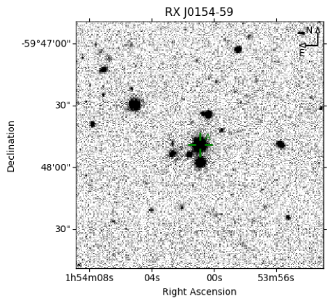
Figure 9: Finding chart for RX J0154.0–5947. Size is 2′$\times$2′. The comparison star is 2″ E and 256″ N of the target and outside the image.

Appendix C Observed times in BJD (TDB)

Table 9: Observed times of optical minima of RX J0154.0–5947 transformed from UTC to BJD (TDB).

Cycle	BJD(TDB)	Error	$O\!-\!C$	Expos	Band	Instr.
	2400000+	(min)	(min)	(min)
-129778	49247.672100	1.4	1.8	2.5	V	(1)
-129777	49247.732600	1.4	0.0	2.5	V	(1)
-129776	49247.795000	1.4	0.9	2.5	V	(1)
-128306	49338.592000	4.3	-0.0	8.0	Spec	(2)
-119106	49906.855400	1.4	-1.1	2.0	V	(3)
-119105	49906.917700	1.4	-0.3	2.0	V	(3)
-119090	49907.844570	1.4	0.2	2.0	V	(3)
-119089	49907.906600	1.4	0.6	2.0	V	(3)
-116841	50046.760000	1.4	-0.1	5.0	Spec	(2)
0	57263.764246	0.7	-0.7	2.0	Sloan r	(4)
1	57263.825894	0.7	-0.9	2.0	Sloan r	(4)
2	57263.888474	0.7	0.3	2.0	Sloan r	(4)
32	57265.740385	0.7	-1.3	1.5	Sloan r	(4)
49	57266.790959	0.7	-0.6	1.5	Sloan r	(4)
50	57266.852630	0.7	-0.7	1.5	Sloan r	(4)
82	57268.830126	0.7	0.6	1.5	Sloan r	(4)
83	57268.892077	0.7	0.9	1.5	Sloan r	(4)
4434	57537.642297	0.7	-0.9	1.0	U	(5)
4514	57542.584319	0.7	-0.0	1.0	Sloan g	(5)
4515	57542.646022	0.7	-0.1	1.0	Sloan g	(5)
4580	57546.661802	1.0	1.2	1.0	WL	(5)
4595	57547.586244	0.9	-1.8	1.0	WL	(5)
4596	57547.648947	0.9	-0.5	1.0	WL	(5)
4675	57552.529255	0.9	0.5	1.0	WL	(5)
4676	57552.590257	0.9	-0.6	1.0	WL	(5)
4774	57558.644130	0.9	0.3	1.0	WL	(5)
11909	57999.356810	1.0	0.1	1.0	Sloan g	(5)
12105	58011.463446	1.0	0.3	1.0	WL	(5)
12168	58015.354383	1.0	-0.3	1.0	WL	(5)
12169	58015.416603	1.0	0.3	1.0	WL	(5)
12170	58015.477993	1.0	-0.2	1.0	WL	(5)
13544	58100.347313	0.7	0.4	1.0	WL	(5)
13546	58100.470187	0.7	-0.5	1.0	WL	(5)
17515	58345.626916	1.0	0.3	1.0	WL	(5)
18273	58392.447349	0.9	1.0	1.0	WL	(5)
18321	58395.411922	0.9	0.6	1.0	WL	(5)
18336	58396.338846	0.9	1.2	1.0	WL	(5)
18337	58396.399895	0.9	0.1	1.0	WL	(5)
18352	58397.327088	0.6	1.1	1.0	WL	(5)

(1) ESO/Dutch 0.9 m, (2) MPI/ESO 2.2m, EFOSC 2, (3) ESO/Danish 2.5 m, (4) ESO 2.2 m, GROND, (5) SAAO MONET/S 1.2 m.

Table 10: Observed times of optical maxima ($m\!=\!+1$) and minima ($m\!=\!-1$) for RX J0600.5–2709 transformed from UTC to BJD(TDB). A maximum and the following minimum have been assigned the same cycle number. The maxima define $\phi\!=\!0$ in Eq. 5, the minima occur on average at $\phi\!=\!0.55$. There may be a cycle count error by one orbit at $E\!=\!-151194$.

Cycle	BJD(TDB)	$m$	Error	$O\!-\!C$	Expos	Band	Instr.
	2400000+		(min)	(min)	(min)
-151194	49753.5883336	$+1$	3.0	-0.5	5.0	V	(1)
-151194	49753.6201522	$-1$	3.0	1.6	5.0	V	(1)
0	58015.5526565	$+1$	3.5	-1.0	1.0	WL	(2)
0	58015.5805583	$-1$	3.5	-4.5	1.0	WL	(2)
1	58015.6067600	$+1$	3.5	-1.8	1.0	WL	(2)

Cycle	BJD(TDB)	$m$	Error	$O\!-\!C$	Expos	Band	Instr.
	2400000+		(min)	(min)	(min)
145	58023.4810547	$+1$	3.8	6.0	1.0	WL	(2)
237	58028.5352205	$-1$	3.5	1.0	1.0	WL	(2)
238	58028.5556718	$+1$	3.5	-4.5	1.0	WL	(2)
238	58028.5917742	$-1$	3.5	3.8	1.0	WL	(2)
239	58028.6126754	$+1$	3.5	-1.1	1.0	WL	(2)
457	58040.5578307	$-1$	4.0	2.1	1.0	WL	(2)
458	58040.5808020	$+1$	3.5	0.2	1.0	WL	(2)
529	58044.4636276	$+1$	5.8	4.6	1.0	WL	(2)
1335	58088.5041883	$+1$	5.8	0.0	1.0	WL	(2)
1353	58089.5192909	$-1$	2.8	1.7	1.0	WL	(2)
1591	58102.5223240	$-1$	2.3	-1.8	1.0	WL	(2)
1592	58102.5501542	$+1$	2.3	3.3	1.0	WL	(2)
1609	58103.5055411	$-1$	2.3	-2.4	1.0	WL	(2)
1610	58103.5334112	$+1$	3.5	2.8	1.0	WL	(2)
1682	58107.4641785	$+1$	2.3	-2.5	1.0	WL	(2)
1682	58107.4964786	$-1$	2.3	0.3	1.0	WL	(2)
1683	58107.5199587	$+1$	2.3	-0.8	1.0	WL	(2)
1683	58107.5511187	$-1$	2.3	0.3	1.0	WL	(2)
1684	58107.5745987	$+1$	2.3	-0.9	1.0	WL	(2)
1734	58110.3364302	$-1$	2.3	-1.9	1.0	WL	(2)
1735	58110.3623902	$+1$	2.3	0.5	1.0	WL	(2)
1735	58110.3945801	$-1$	2.3	3.1	1.0	WL	(2)
1736	58110.4444301	$-1$	3.5	-3.8	1.0	WL	(2)
1737	58110.4682301	$+1$	2.3	-4.5	1.0	WL	(2)
1737	58110.4993300	$-1$	2.3	-3.4	1.0	WL	(2)
1738	58110.5268300	$+1$	2.3	1.2	1.0	WL	(2)
1755	58111.4844283	$-1$	2.3	-1.3	1.0	WL	(2)
1810	58114.4585864	$+1$	2.3	-2.7	1.0	WL	(2)
1810	58114.4918062	$-1$	2.3	1.5	1.0	WL	(2)
1811	58114.5129561	$+1$	3.5	-3.1	1.0	WL	(2)
1811	58114.5445258	$-1$	2.3	-1.3	1.0	WL	(2)
1812	58114.5679957	$+1$	2.3	-2.5	1.0	WL	(2)
2814	58169.3232900	$+1$	2.3	-0.7	1.0	WL	(2)
2816	58169.4332140	$+1$	2.3	0.2	1.0	WL	(2)
3929	58230.2839183	$-1$	2.3	1.2	1.0	WL	(2)
3947	58231.2688652	$-1$	2.3	3.1	1.0	WL	(2)
6058	58346.5885790	$+1$	3.5	-4.2	1.0	WL	(2)
6058	58346.6193800	$-1$	3.5	-3.6	1.0	WL	(2)
7483	58424.4891501	$-1$	1.7	-2.2	1.0	WL	(2)
7484	58424.5162715	$+1$	1.7	1.9	1.0	WL	(2)
7631	58432.5453950	$+1$	1.7	-3.4	1.0	WL	(2)
7631	58432.5775760	$-1$	1.7	-0.8	1.0	WL	(2)
7722	58437.5236975	$+1$	2.3	4.7	1.0	WL	(2)
7722	58437.5493075	$-1$	2.3	-2.1	1.0	WL	(2)
8523	58481.3225700	$-1$	1.2	1.9	1.0	WL	(2)
8524	58481.3450900	$+1$	1.2	-0.7	1.0	WL	(2)
8524	58481.3774100	$-1$	1.2	2.2	1.0	WL	(2)
8596	58485.3102370	$-1$	1.2	-0.1	1.0	WL	(2)
8597	58485.3346220	$+1$	1.2	-0.0	1.0	WL	(2)
8597	58485.3655300	$-1$	1.2	0.8	1.0	WL	(2)
8765	58494.5160935	$+1$	1.2	1.6	1.0	WL	(2)
8765	58494.5440108	$-1$	1.2	-1.9	1.0	WL	(2)
8766	58494.5707000	$+1$	1.2	1.6	1.0	WL	(2)
8819	58497.4970370	$-1$	1.2	1.3	1.0	WL	(2)
8820	58497.5206460	$+1$	1.2	0.3	1.0	WL	(2)
8820	58497.5517050	$-1$	1.2	1.3	1.0	WL	(2)
9127	58514.3250900	$-1$	1.7	-2.4	1.0	WL	(2)
9128	58514.3493900	$+1$	1.7	-2.4	1.0	WL	(2)
9128	58514.3799800	$-1$	1.7	-2.0	1.0	WL	(2)

(1) ESO/Dutch 0.9 m, (2) SAAO MONET/S 1.2 m

Table 11: Observed times of optical minima for RX J0859.1+0537 transformed from UTC to BJD(TDB).

Cycle	BJD(TDB)	Error	$O\!-\!C$	Expos	Band	Instr.
	2400000+	(min)	(min)	(min)
-51517	50097.645900	2.9	1.3	0.5	V	(1)
-51516	50097.744854	1.0	-0.1	0.5	V	(1)
-51515	50097.843176	2.9	-2.4	0.5	V	(1)
0	55246.837490	3.6	0.3	1.0	WL	(2)
2643	55511.009128	1.8	0.7	1.0	WL	(2)
2662	55512.908370	2.3	1.0	1.0	WL	(2)
2663	55513.008100	2.7	0.7	1.0	WL	(2)
2722	55518.904510	4.5	-0.4	1.0	WL	(2)
2723	55519.006940	2.9	3.2	1.0	WL	(2)
2841	55530.798980	1.4	-0.0	1.0	WL	(2)
2842	55530.898890	1.4	-0.1	1.0	WL	(2)
2872	55533.895720	2.7	-2.5	1.0	WL	(2)
2962	55542.893854	2.7	1.1	1.0	WL	(2)
3132	55559.885170	1.4	0.5	1.0	WL	(2)
4061	55652.740434	2.3	1.2	1.0	WL	(2)
6454	55891.925500	2.9	3.4	1.0	WL	(2)
16989	56944.910430	2.9	0.2	1.0	WL	(2)
18028	57048.758480	1.4	-1.8	1.0	WL	(2)
18058	57051.757280	1.4	-1.4	1.0	WL	(2)
29250	58170.412259	1.7	-1.7	1.0	WL	(3)
29369	58182.306969	1.4	-1.0	1.0	WL	(3)
32282	58473.466899	1.4	1.5	1.0	WL	(3)
32552	58500.452806	1.4	0.1	1.0	WL	(3)
32562	58501.453029	1.4	1.1	1.0	WL	(3)

(1) ESO/Dutch 0.9 m, (2) McDonald Observatory MONET/N 1.2 m, (2) SAAO MONET/S 1.2 m.

Table 12: Observed times of the center of the optical bright phase for RX J0953.1+1458 transformed from UTC to BJD(TDB).

Cycle	BJD(TDB)	Error	$O\!-\!C$	Expos	Band	Instr.
	2400000+	(min)	(min)	(min)
-75884	49752.612917	0.9	-0.4	4.0	V	(1)
-40714	52285.641017	0.4	-0.0	1.0	WL	(2)
-40713	52285.713156	0.4	0.2	1.0	WL	(2)
-39773	52353.413600	0.6	-0.7	3.0	WL	(3)
0	55217.961107	0.4	0.1	1.0	WL	(4)
388	55245.906033	0.4	0.4	1.0	WL	(4)
389	55245.977962	0.4	0.3	1.0	WL	(4)
444	55249.939017	0.4	0.0	1.0	WL	(4)
4193	55519.951229	0.4	0.4	1.0	WL	(4)
4430	55537.020418	0.4	0.2	1.0	WL	(4)
5803	55635.906705	0.4	-0.5	1.0	WL	(4)
9261	55884.959682	0.6	-1.2	1.0	WL	(4)
24353	56971.922940	0.6	0.5	1.0	WL	(4)
25616	57062.886273	0.6	-0.8	1.0	WL	(4)
41021	58172.391979	0.4	0.0	1.0	WL	(5)
41175	58183.482879	0.6	-0.7	1.0	WL	(5)
45730	58511.545461	0.4	0.0	1.0	WL	(5)
45758	58513.562168	0.4	0.2	1.0	WL	(5)

(1) ESO/Dutch 0.9 m, (2) Calar Alto 3.5 m OPTIMA (Kanbach et al. 2008), (3) Observatorio Astronómico de Mallorca, 30-cm, (4) McDonald Observatory MONET/N 1.2 m, (5) SAAO MONET/S 1.2 m.

Table 13: Observed times of the X-ray dips and the primary optical minima of RX J1002.2–1925 transformed from UTC to BJD(TDB). The minima included in the fit for Eq. 8 have $i7\!=\!1$, those for Eq. 9 have $i8\!=\!1$. The $O\!-\!C$ values are correlated with the WL AB magnitude $w$.

Cycle	BJD(TDB)	Error	i7	$O\!-\!C$	i8	$O\!-\!C$	Exp	Band	$w$	Instr.
	2400000+			Eq. 8		Eq. 9
		(min)		(min)		(min)	(min)		(mag)
-58114	48219.66788	1.9	1	-1.4	1	0.7	0.5	X		(1)
-47122	48982.81668	2.5	1	0.3	1	1.5	10.0	Sp		(2)
-36074	49749.85143	1.4	1	-1.0	1	-0.7	2.5	V		(3)
-34287	49873.91908	0.9	1	-0.1	1	0.0	0.9	X		(4)
-34286	49873.98852	0.9	1	-0.1	1	0.1	0.9	X		(4)
-25144	50508.69555	1.8	1	0.4	1	-0.2	10.0	Sp		(2)
-25130	50509.66776	2.5	1	0.7	1	0.1	10.0	Sp		(2)
0	52254.38165	0.7	1	-0.0	0	-2.7	0.3	X		(5)
0	52254.38211	0.7	1	0.6	0	-2.1	1.0	X		(6)
43087	55245.80718	1.7	1	0.7	0	-5.5	1.0	WL	16.69	(7)
47381	55543.93358	2.9	0	7.2	1	0.6	1.0	WL	19.17	(7)
47396	55544.97553	1.7	0	8.0	1	1.4	1.0	WL	19.09	(7)
47754	55569.82950	1.4	0	6.4	1	-0.2	1.0	WL	19.07	(7)
47757	55570.03700	1.4	0	5.3	1	-1.4	1.0	WL	18.76	(7)
48157	55597.81030	1.9	0	8.6	1	1.9	1.0	WL	18.87	(7)
48947	55652.65544	1.4	0	4.8	1	-2.0	1.0	WL	17.96	(7)
68353	56999.96355	2.3	1	0.5	0	-7.9	1.0	WL	17.57	(7)
76308	57552.25820	1.4	1	-1.7	0	-10.8	1.0	WL	17.60	(8)
76309	57552.32788	1.4	1	-1.4	0	-10.4	1.0	WL	17.48	(8)
76538	57568.22837	1.2	1	0.9	0	-8.1	1.0	WL	17.53	(8)
76610	57573.22657	1.2	1	0.1	0	-9.0	1.0	WL	17.48	(8)
80528	57845.24718	1.4	0	5.0	1	-4.3	1.0	WL	18.60	(8)
85210	58170.31063	1.7	0	10.3	1	0.5	1.0	WL	18.84	(8)
85282	58175.31047	1.7	0	11.8	1	2.1	1.0	WL	18.74	(8)
85283	58175.37911	1.4	0	10.7	1	0.9	1.0	WL	18.78	(8)
85958	58222.24217	1.7	0	9.9	1	0.1	1.0	WL	18.89	(8)
85987	58224.25517	1.4	0	9.3	1	-0.5	1.0	WL	18.80	(8)
86045	58228.28154	1.4	0	8.7	1	-1.1	1.0	WL	18.90	(8)
86261	58243.28102	1.4	0	13.2	1	3.4	1.0	WL	18.95	(8)
86277	58244.39114	1.4	0	12.2	1	2.3	1.0	WL	18.87	(8)
86289	58245.22339	2.0	0	10.9	1	1.1	1.0	WL	18.77	(8)
86290	58245.29243	2.0	0	10.3	1	0.5	1.0	WL	18.90	(8)
89174	58445.51451	2.9	1	0.3	0	-9.8	1.0	WL	17.99	(8)
89994	58502.45117	2.0	0	9.0	1	-1.1	1.0	WL	18.45	(8)
90008	58503.42288	2.0	0	8.6	1	-1.5	1.0	WL	18.44	(8)
90009	58503.49290	2.0	0	9.5	1	-0.7	1.0	WL	18.40	(8)
90010	58503.56170	2.0	0	8.6	1	-1.6	1.0	WL	18.40	(8)

(1) RASS PSPC, (2) MPI/ESO/ 2.2 m EFOSC2, spectrophotometry, (3) ESO/Dutch 0.9 m, (4) ROSAT HRI, (5) XMM-Newton EPIC pn, (6) XMM-Newton EPIC MOS12, (7) McDonald Observatory MONET/N 1.2 m, (8) SAAO MONET/S 1.2 m.