Symbolic Self-triggered Control of Continuous-time Non-deterministic Systems without Stability Assumptions for 2-LTL Specifications

Abstract

We propose a symbolic self-triggered controller synthesis procedure for non-deterministic continuous-time nonlinear systems without stability assumptions. The goal is to compute a controller that satisfies two objectives. The first objective is represented as a specification in a fragment of LTL, which we call 2-LTL. The second one is an energy objective, in the sense that control inputs are issued only when necessary, which saves energy. To this end, we first quantise the state and input spaces, and then translate the controller synthesis problem to the computation of a winning strategy in a mean-payoff parity game. We illustrate the feasibility of our method on the example of a navigating nonholonomic robot.

I Introduction

Not only has self-triggered control been a hot academic research topic in recent years, but it also provides a variety of practical implementations [1]. By performing sensing and actuation only when needed, self-triggered control is well-known as an energy-aware control paradigm to save communication resources for Networked Control Systems [2]. The lifespan of battery-powered devices can be prolonged by reducing their energy consumption [1] and the communication load of nonholonomic robots significantly reduced in comparison to using periodic controllers [3]. However, previous research on self-triggered control of continuous-time systems only studies simple specifications such as stability [4] and reach-avoid or safety problems [5, 6].

The main reason for this limitation is that those approaches are based on reachability analysis. The main novelty of our work is to use techniques from game theory to go beyond reach-avoid and safety specifications for self-triggered control. Game theory, and in particular parity games [7], is a well-known technique to deal with expressive logic like the $\mu$-calculus [7] and $\text{CTL}^{*}$ [8], as the parity winning conditions provide complex scenarios and strategies while keeping computability. In particular, parity games can be used for control synthesis of reactive systems under Linear Temporal Logic (LTL) specifications [9]. On the other hand, quantitative games such as mean-payoff games [10] have been adapted to quantitative control specifications [11, 12]. One of such specifications is the mean-payoff threshold problem for the average control-signal length of self-triggered controllers. This threshold provides guarantees for the energy-saving and communication-reduction performance of the controller: the greater the average length of a signal is, the less often the controller needs to perform sensing and actuation, and fewer commands are sent across the network. In this paper, we deal with this threshold problem together with a logical specification using mean-payoff parity games, which combine mean-payoff games and parity games. The logical specifications can be dealt with the parity side, while the average signal length threshold can be seen as a threshold problem in a mean-payoff game.

Our procedure is based on the symbolic control approach, which synthesises correct-by-design controllers of continuous-state systems. In this approach, we first construct a symbolic model, which is a discrete abstraction of the continuous-state system, based on approximate simulation or bisimulation. Then, we synthesise a symbolic controller and leverage its control strategy to control the continuous-state system. This technique allows us to synthesise provably-correct controllers for complex specification such as LTL specifications, which can hardly be enforced with conventional control methods. However, previous symbolic control algorithms for continuous-time nonlinear systems under LTL specifications need stability assumptions (e.g., [13, 14]), which do not hold in many systems. Symbolic control without stability assumptions is enforced on simpler classes of specifications such as reach-avoid [5, 15, 16]. The work closest to ours is [5], in which the authors propose an algorithm to synthesise symbolic self-triggered controllers for discrete-time deterministic systems under reach-avoid specifications.

This work proposes a symbolic self-triggered control procedure for continuous-time non-deterministic nonlinear systems without stability assumptions for specifications represented by a fragment of LTL, which we call 2-LTL. To the best of our knowledge, our work is the first to study symbolic control of continuous-time nonlinear systems without stability assumptions for a class of LTL specifications that is strictly more expressive than reach-avoid. Our procedure operates in several steps: (1) constructing a finite symbolic model of the continuous system, (2) translating the self-triggered controller synthesis problem on the symbolic model into a mean-payoff parity game problem, (3) constructing a winning strategy for the mean-payoff parity game, (4) translating the strategy back into a controller for the symbolic model, and (5) translating the controller for the symbolic model back into one for the continuous system.

Notation: We denote vectors in $\mathbb{R}^{m}$ by $x=\begin{bmatrix}x_{1}&\cdots&x_{m}\end{bmatrix}^{\intercal}$. For such a vector $x$, we use $\lVert x\rVert$ for its infinity norm $\max\,\{\,\lvert x_{i}\rvert~{}\mid\,i\in\{1,\ldots,m\}\}$. Given $x\in\mathbb{R}^{m}$ and $r\in\mathbb{R}_{>0}$, we write $\mathcal{B}_{r}(x)$ for the ball $\{y\in\mathbb{R}^{m}\,\mid\,\lVert x-y\rVert\leq r\}$ of centre $x$ and radius $r$. Finally, given a set $X$, we denote its powerset $\{Y\,\mid\,Y\subseteq X\}$ by ${\wp}(X)$.

II Control Framework

II-A System

We formalise a non-deterministic continuous-time nonlinear system as a 6-tuple $\Sigma=(X,X_{\text{in}},U,{{\mathcal{U}}},\xi^{\rightarrow},\xi^{\leftarrow}),$ where $X\subseteq{\mathbb{R}}^{n}$ is a bounded convex state space, $X_{\text{in}}\subseteq X$ is a space of initial states, $U\subseteq{{\mathbb{R}}}^{m}$ is a bounded convex space of control inputs, ${{\mathcal{U}}}$ is a set of control signals of the form $[0,T]\to U$ that assign a control input at each time in the interval $[0,T]$ with $T\in{\mathbb{R}}_{>0}$, and $\xi^{\rightarrow}$, $\xi^{\leftarrow}$ $:{\mathbb{R}}^{n}\times{\mathcal{U}}\times{\mathbb{R}}_{\geq 0}\to{\wp}({\mathbb{R}}^{n})$ are functions such that $\xi_{x,u}^{\rightarrow}(0)=\xi_{x,u}^{\leftarrow}(0)=\{x\}$. Intuitively, given a state $x\in{\mathbb{R}}^{n}$, a signal $u\in{\mathcal{U}}$, and a time $t\geq 0$, $\xi_{x,u}^{\rightarrow}(t)$ (resp. $\xi_{x,u}^{\leftarrow}(t)$) is the reachable states from $x$ (resp. the set of states from which the system can reach $x$) under the control signal $u$ at time $t$.

The system is defined on the whole Euclidean space ${\mathbb{R}}^{n}$, but we are only interested in its behaviour on a bounded subspace $X$ because the quantities involved in systems are physically bounded, as observed in [16]. For technical reasons, we also assume that the distance from $X_{\text{in}}$ to the boundary of $X$ is positive.

The system $\Sigma$ is said to be forward and backward complete [17] if $\xi_{x,u}^{\rightarrow}(t)\neq\emptyset$ and $\xi_{x,u}^{\leftarrow}(t)\neq\emptyset$ for all $(x,u)\in{\mathbb{R}}^{n}\times{\mathcal{U}}$ and all $t\in[0,{{\text{len}}}(u)]$, where ${{\text{len}}}(u)=T$ is the length of the signal $u:[0,T]\to U$. In other words, under any control signal, there exist a state reachable from $x$ and a state that reaches $x$ at any time within the signal length.

Definition 1.

A system $\Sigma$ is incrementally forward and backward complete if it is forward and backward complete, and, for each $u\in{\mathcal{U}}$, there exist functions $\beta^{\rightarrow}_{u},\beta^{\leftarrow}_{u}:{\mathbb{R}}_{\geq 0}\times{\mathbb{R}}_{\geq 0}\to{\mathbb{R}}_{\geq 0}$ such that 1) for any $t\in{\mathbb{R}}_{\geq 0}$, $\beta^{\rightarrow}_{u}(\_,t)$ and $\beta^{\leftarrow}_{u}(\_,t)$ are strictly increasing and their limits at $+\infty$ is $+\infty$, and 2) for any $x_{1},x_{2}\in{\mathbb{R}}^{n}$, $u\in{{\mathcal{U}}}$, and $t\leq{{\text{len}}}(u)$,

1. $\forall(x_{1}^{\prime},x_{2}^{\prime})\in\xi^{\rightarrow}_{x_{1},u}(t)\times\xi^{\rightarrow}_{x_{2},u}(t),\lVert x_{1}^{\prime}-x_{2}^{\prime}\rVert\leq\beta^{\rightarrow}_{u}(\lVert x_{1}-x_{2}\rVert,t)\hbox to0.0pt{,\hss}$

2. $\forall(x_{1}^{\prime},x_{2}^{\prime})\in\xi^{\leftarrow}_{x_{1},u}(t)\times\xi^{\leftarrow}_{x_{2},u}(t),\lVert x_{1}^{\prime}-x_{2}^{\prime}\rVert\leq\beta^{\leftarrow}_{u}(\lVert x_{1}-x_{2}\rVert,t)\hbox to0.0pt{.\hss}$

Notice that incremental forward and backward completeness does not depend on the state space $X$, but on ${\mathbb{R}}^{n}$. There may exists $(x,u)\in X\times{\mathcal{U}}$ such that $\xi^{\rightarrow}_{x,u}(t)\cap X=\emptyset$, i.e., the system runs out of the desired state space.

Assumption 1.

The system $\Sigma$ is incrementally forward and backward complete.

Assumption 1 is similar to the one used in [16], but adapted to non-deterministic systems and taking backward dynamics into account. The intuition behind Assumption 1 is that the distance between the states reached from two starting points can be bound by an expression that depends only on the distance between those starting points, the control signal, and the run time. In addition, we require the following assumption.

Assumption 2.

For any control signal $u\in{\mathcal{U}}$, we have functions $\alpha^{\rightarrow}_{u},\alpha^{\leftarrow}_{u}:{\mathbb{R}}_{\geq 0}\times[0,{{\text{len}}}(u)]\to{\mathbb{R}}_{\geq 0}$ such that 1) for any $t\in{\mathbb{R}}_{\geq 0}$, $\alpha^{\rightarrow}_{u}(\_,t)$ and $\alpha^{\leftarrow}_{u}(\_,t)$ are increasing, and 2) for any $x_{1},x_{2}\in X$ and any $t\in[0,{{\text{len}}}(u)]$, we have

1. for any $y_{2}\in\xi_{x_{2},u}^{\rightarrow}(t),\rVert x_{1}-y_{2}\lVert\leq\alpha^{\rightarrow}_{u}(\rVert x_{1}-x_{2}\lVert,t)\hbox to0.0pt{,\hss}$

2. for any $y_{2}\in\xi_{x_{2},u}^{\leftarrow}(t),\rVert x_{1}-y_{2}\lVert\leq\alpha^{\leftarrow}_{u}(\rVert x_{1}-x_{2}\lVert,t)\hbox to0.0pt{.\hss}$

Assumption 2 basically states that the set of reachable states cannot be arbitrarily far from the starting state (for a given input signal and run time). Those functions $\beta^{\rightarrow}_{u}$, $\beta^{\leftarrow}_{u}$, $\alpha^{\rightarrow}_{u}$, and $\alpha^{\leftarrow}_{u}$ can typically be computed using Lyapunov functions (see [16, 17, 18] for details).

II-B State-transition Model

Let us first introduce general definitions for state-transition models and their controllers. For this paper, a state-transition model is given by a quadruple ${\mathcal{M}}=(Y,Y_{\text{in}},\mathcal{V},\rightarrow),$ where $Y$ is either a continuous or a discrete state space, $Y_{\text{in}}\subseteq Y$ is a set of initial states, $\mathcal{V}$ is a set of control signals, and $\rightarrow\,\subseteq Y\times\mathcal{V}\times Y$ is the transition relation. For a given state $y\in Y$, a sequence $y_{0}u_{0}y_{1}u_{1}\ldots\in Y(\mathcal{V}Y)^{\omega}$ (resp. $y_{0}u_{0}y_{1}\ldots u_{l-1}y_{l}\in Y(\mathcal{V}Y)^{*}$) is a run (resp. a finite run) generated by ${\mathcal{M}}$ starting from the state $y$ if $y_{0}=y$ and $(y_{i},u_{i},y_{i+1})\in\to$ for any $i\in\mathbb{Z}_{\geq 0}$ (resp. $i\in\{0,\ldots,l-1\}$). Let $\mathit{Run}({\mathcal{M}},y)$ (resp. $\mathit{FRun}({\mathcal{M}},y)$) denote the set of all runs (resp. finite runs) generated by ${\mathcal{M}}$ from $y$. Let $\mathit{Run}({\mathcal{M}})=\bigcup_{y\in Y_{\text{in}}}\mathit{Run}({\mathcal{M}},y)$ and $\mathit{FRun}({\mathcal{M}})=\bigcup_{y\in Y_{\text{in}}}\mathit{FRun}({\mathcal{M}},y)$.

We define the state-transition model of $\Sigma$ as follows.

Definition 2.

The state-transition model ${\mathcal{M}}(\Sigma)$ of a system $\Sigma=(X,X_{\text{in}},U,{{\mathcal{U}}},\xi^{\rightarrow},\xi^{\leftarrow})$ is ${\mathcal{M}}(\Sigma)=(X,X_{\text{in}},{\mathcal{U}},\Delta),$ where the transition relation $\Delta\subseteq X\times{\mathcal{U}}\times X$ is given by

$$(x,u,x^{\prime})\in\Delta\text{~{}iff~{}} x^{\prime}\in\xi_{x,u}^{\rightarrow}({{\text{len}}}(u))\text{,~{}}x\in\xi_{x^{\prime},u}^{\leftarrow}({{\text{len}}}(u))$$

 and, for all $$t\leq{{\text{len}}}(u) \xi^{\rightarrow}_{x,u}(t)\subseteq X$$, .

Runs of a model are discrete sequences of states, but the system runs in continuous time. In order to fill this gap, we introduce the notion of trajectory to match these discrete runs to continuous sequences of states.

Definition 3.

A trajectory of a system $\Sigma$ starting from a state $x\in X$ induced by a run $x_{0}u_{0}x_{1}u_{1}x_{2}\ldots\in\mathit{Run}({\mathcal{M}}(\Sigma),x)$ is a function $\sigma:{\mathbb{R}}_{\geq 0}\to X$ such that, for all $k\in\mathbb{Z}_{\geq 0}$ and all $t\in\big{[}\sum_{i<k}{{\text{len}}}(u_{i}),\sum_{i\leq k}{{\text{len}}}(u_{i})\big{]}$,

$$\sigma (t)\in\xi_{x_{k},u_{k}}^{\rightarrow}\big{(}t-\sum_{i<k}{{\text{len}}}(u_{i})\big{)}\cap\xi_{x_{k+1},u_{k}^{\prime}}^{\leftarrow}\big{(}\sum_{i\leq k}{{\text{len}}}(u_{i})-t\big{)},$$

$$\text{where }u_{k}^{\prime}(s)=u_{k}\big{(}s+t-\displaystyle\sum_{i<k}{{\text{len}}}(u_{i})\big{)},\forall s\in[0,\displaystyle\sum_{i\leq k}{{\text{len}}}(u_{i})-t].$$

Let $\mathit{Traj}(\Sigma,x,r)$ be the set of trajectories of $\Sigma$ that are induced by a run $r\in\mathit{Run}({\mathcal{M}}(\Sigma),x)$. For any finite run $r_{f}\in\mathit{FRun}({\mathcal{M}}(\Sigma),x)$, $\mathit{FTraj}(\Sigma,x,r_{f})$ is the set of finite trajectories defined in the same way. Let $\mathit{Traj}(\Sigma,x)=\bigcup_{r\in\mathit{Run}({\mathcal{M}}(\Sigma),x)}\mathit{Traj}(\Sigma,x,r)$, and $\mathit{Traj}(\Sigma)=\bigcup_{x\in X_{\text{in}}}\mathit{Traj}(\Sigma,x)$.

II-C Controlled System

In this section, we define controllers and controlled systems, and explain the self-triggered control process. First, we define model controllers of ${\mathcal{M}}=(Y,Y_{\text{in}},\mathcal{V},\rightarrow)$.

Definition 4.

A model controller of a state-transition model ${\mathcal{M}}$ is a function $\mathcal{C}:\mathit{FRun}({\mathcal{M}})\to\mathcal{V}$.

Let ${\mathcal{C}}/{{\mathcal{M}}}$ denote the state-transition model ${\mathcal{M}}$ controlled under $\mathcal{C}$. A run $y_{0}u_{0}y_{1}\ldots\in\mathit{FRun}({\mathcal{M}},y)$ (resp. a finite run $y_{0}u_{0}y_{1}\ldots u_{l-1}y_{l}\in\mathit{Run}({\mathcal{M}},y)$) is generated by ${\mathcal{C}}/{{\mathcal{M}}}$ if it satisfies the following conditions: 1) $y_{0}=y$, and 2) for all $i\in\mathbb{Z}_{\geq 0}$ (resp. for all $i\in[0,l-1]$), we have $u_{i}=\mathcal{C}(y_{0}u_{0}\ldots y_{i})$. Then, let $\mathit{Run}({\mathcal{C}}/{{\mathcal{M}}},y)$ (resp. $\mathit{FRun}({\mathcal{C}}/{{\mathcal{M}}},y)$) denotes the set of all runs (resp. finite runs) generated by ${\mathcal{C}}/{{\mathcal{M}}}$ from $y\in Y$. Let $\mathit{Run}({\mathcal{C}}/{{\mathcal{M}}})=\bigcup_{y\in Y_{\text{in}}}\mathit{Run}({\mathcal{C}}/{{\mathcal{M}}},y)$ and $\mathit{FRun}({\mathcal{C}}/{{\mathcal{M}}})=\bigcup_{y\in Y_{\text{in}}}\mathit{FRun}({\mathcal{C}}/{{\mathcal{M}}},y)$.

Definition 5.

A controller of $\Sigma=(X,X_{\text{in}},U,{{\mathcal{U}}},\xi^{\rightarrow},\xi^{\leftarrow})$ is a function $C:\mathit{FRun}({\mathcal{M}}(\Sigma))\to{\mathcal{U}}$.

Notice that a controller $C$ of a system $\Sigma$ is defined based on its state-transition model ${\mathcal{M}}(\Sigma)$. This is because the controller issues control signals based on runs, which only track the states at the end of each signal. Since Definition 5 is coherent with Definition 4, we can also regard $C$ as a model controller of ${\mathcal{M}}(\Sigma)$. Hence, we also use $\mathit{Run}({C}/{{\mathcal{M}}(\Sigma)})$ (resp. $\mathit{FRun}({C}/{{\mathcal{M}}(\Sigma)})$) to denote the sets of runs (resp. finite runs) of ${C}/{{\mathcal{M}}(\Sigma)}$ from initial states. Furthermore, we use ${C}/{\Sigma}$ to denote the system $\Sigma$ controlled under the controller $C$, and define the trajectories of ${C}/{\Sigma}$ in the same way as in Definition 3. Thereby, the definitions of trajectories $\mathit{Traj}({C}/{\Sigma})$ and $\mathit{FTraj}({C}/{\Sigma})$ carry over to controlled systems directly.

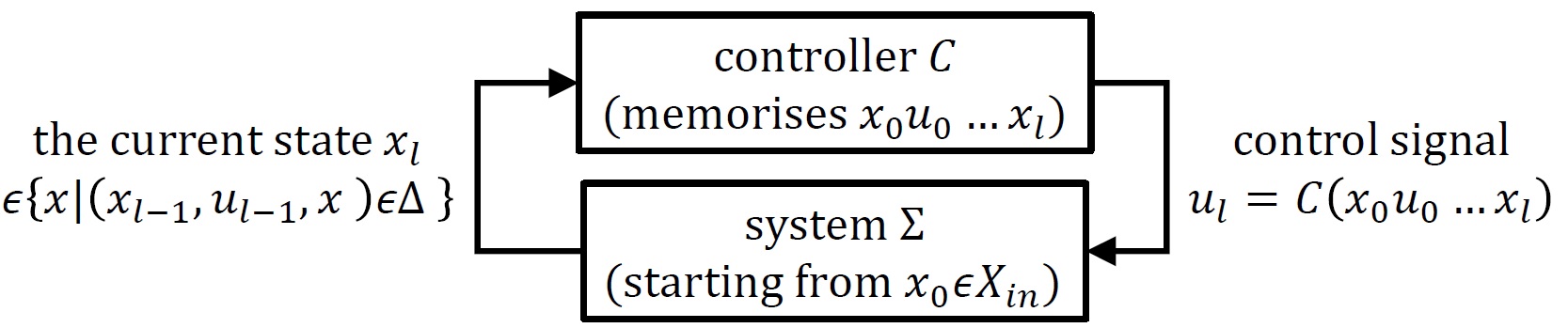
Figure 1: Overview of the self-triggered control process. Based on previously observed states and issued control signals, the controller issues a control signals to control the system.

The overview of the control process is illustrated in Fig 1. First, the controller observes the initial state $x_{0}\in X_{\text{in}}$ and issues the control signal $u_{0}=C(x_{0})$. Then, to preserve energy, the controller is inactive throughout the duration of the control signal $u_{0}$. Namely, the longer the signal length ${{\text{len}}}(u_{0})$ is, the more energy is preserved. Since the system is non-deterministic, there are several states that can possibly be reached under the signal $u_{0}$. After the signal ends (at time ${{\text{len}}}(u_{0})$), the controller becomes active and resolves the non-determinism by detecting the actual current state $x_{1}$ and issue a new control signal $u_{1}=C(x_{0}u_{0}x_{1})$. The process is then repeated.

III Problem Formulation

Our goal is to synthesise a controller that satisfies two control objectives. The first objective is described as a $\operatorname{2-LTL}$ formula. The second one is an energy-preservation objective: to ensure that the average length of the issued control signals is above a given threshold.

III-A $\operatorname{2-LTL}$ Specification

We model the first objective using a fragment of LTL, which we call $\operatorname{2-LTL}$. Let $AP$ denote the set of atomic propositions, i.e., assertions that can be either true or false at each state $x\in X$. Let $P:X\to{\wp}(AP)$ assign the set of atomic propositions that hold at each state.

Definition 6.

Let $\operatorname{2-LTL}$ be the logic whose formulas are the $\Phi$’s generated by the following grammar:

$$\varphi \Coloneqq\top\mid p\mid\neg\varphi\mid\varphi\vee\varphi$$

$$\Phi \Coloneqq\Diamond\varphi\mid\Box\varphi\mid\Box\Diamond\varphi\mid\Diamond\Box\varphi\mid\Phi\vee\Phi\mid\Phi\wedge\Phi\hbox to0.0pt{,\hss}$$

where $p\in AP$ is an atomic proposition.

We call $\varphi$’s and $\Phi$’s state formulas and path formulas, respectively. A logic specification is written as a path formula. Here, $\Box$ and $\Diamond$ have the usual interpretation of LTL. A state $x\in X$ satisfying (resp. not satisfying) a state formula $\varphi$ is denoted by $x\vDash\varphi$ (resp. $x\not\vDash\varphi$). We also use the same notations $\sigma\vDash\Phi$ and $\sigma\not\vDash\Phi$ for a trajectory $\sigma:{\mathbb{R}}_{\geq 0}\to X$ and a path formula $\Phi$. For every state $x\in X$, $x\vDash\varphi$ is defined as follows:

$$x \vDash\top x \vDash p\text{ if }p\in P(x)$$

$$x \vDash\neg\varphi\text{ if }x\not\vDash\varphi x \vDash\varphi_{1}\vee\varphi_{2}\text{ if }x\vDash\varphi_{1}\text{ or }x\vDash\varphi_{2}\hbox to0.0pt{,\hss}$$

and for all $\sigma:{\mathbb{R}}_{\geq 0}\to X$, $\sigma\vDash\Phi$ is defined as follows:

$$\sigma \vDash\Diamond\varphi\text{~{}~{}if~{}~{}}\exists t\in{\mathbb{R}}_{\geq 0},\,\sigma(t)\vDash\varphi$$

$$\sigma \vDash\Box\varphi\text{~{}~{}if~{}~{}}\forall t\in{\mathbb{R}}_{\geq 0},\,\sigma(t)\vDash\varphi$$

$$\sigma \vDash\Box\Diamond\varphi\text{~{}~{}if~{}~{}}\forall t\in{\mathbb{R}}_{\geq 0},\,\exists t^{\prime}>t,\,\sigma(t^{\prime})\vDash\varphi$$

$$\sigma \vDash\Diamond\Box\varphi\text{~{}~{}if~{}~{}}\exists t\in{\mathbb{R}}_{\geq 0},\,\forall t^{\prime}>t,\,\sigma(t^{\prime})\vDash\varphi$$

$$\sigma \vDash\Phi_{1}\vee\Phi_{2}\text{~{}~{}if~{}~{}}\sigma\vDash\Phi_{1}\text{ or }\sigma\vDash\Phi_{2}$$

$$\sigma \vDash\Phi_{1}\wedge\Phi_{2}\text{~{}~{}if~{}~{}}\sigma\vDash\Phi_{1}\text{ and }\sigma\vDash\Phi_{2}\hbox to0.0pt{.\hss}$$

One objective of a controller $C$ is to control the system in such a way that all trajectories in $\mathit{Traj}({C}/{\Sigma})$ satisfy a given $\operatorname{2-LTL}$ path formula $\Phi$. Notice that the class of $\operatorname{2-LTL}$ specifications is more general than the reach-avoid specifications, which is studied in [5, 15, 6]. For example, we can express the logic specification to reach $\mathtt{target\_region}$ while avoiding $\mathtt{unsafe\_region}$ using the $\operatorname{2-LTL}$ formula $\Diamond\mathtt{target\_region}\wedge\Box\neg\mathtt{unsafe\_region}$.

III-B Controller Synthesis Problem

Definition 7.

Given a system $\Sigma=(X,X_{\text{in}},U,{{\mathcal{U}}},\xi^{\rightarrow},\xi^{\leftarrow})$, a set $AP$ of atomic propositions, a function $P:X\to{\wp}(AP)$, a $\operatorname{2-LTL}$ formula $\Phi$, and a threshold $\nu\in{\mathbb{R}}_{>0}$, the controller synthesis problem is to synthesise a controller $C:\mathit{FRun}({\mathcal{M}}(\Sigma))\to{\mathcal{U}}$ such that

• all finite runs in $\mathit{FRun}({C}/{{\mathcal{M}}(\Sigma)})$ can be extended to an infinite run in $\mathit{Run}({\mathcal{M}}(\Sigma))$,

• $\sigma\vDash\Phi$ for any $\sigma\in\mathit{Traj}({C}/{\Sigma})$, and

• $\displaystyle\lim_{h\to\infty}\frac{1}{h}\sum_{i=1}^{h}{{\text{len}}}(u_{i})>\nu$ for any $x_{0}u_{0}\ldots\in\mathit{Run}({C}/{{\mathcal{M}}(\Sigma)})$,

or determine that such a controller $C$ does not exist.

The first condition simply ensures that the controlled system does not reach a deadlock, while the other two conditions are the actual control objectives.

IV Problem Reduction to Symbolic Control

In this section, we state our symbolic controller synthesis problem, which considers a discrete system obtained by quantising states and inputs, and by restricting control signals to piecewise-constant ones. We show that a symbolic controller for this problem also satisfies the conditions in Definition 7.

IV-A Piecewise-constant Control Signal with Discrete Input

For a given bounded convex control input space $U\subseteq{\mathbb{R}}^{m}$ and a discretisation parameter $\mu\in{\mathbb{R}}_{>0}$, let

$$U_{\mu}=\big{\{}\begin{bmatrix}u_{1}&\cdots&u_{m}\end{bmatrix}^{\intercal}\in U\bigm{|}u_{i}=2\mu l_{i},\ l_{i}\in{\mathbb{Z}},\ i\leq m\big{\}}$$ (1)

be the quantised input set by an $m$-dimensional hypercube of $2\mu$ edge length. As $U$ is bounded, $U_{\mu}$ is finite.

Given $\tau\in{\mathbb{R}}_{>0}$ and $\ell=[\ell_{\text{min}},\ell_{\text{max}}]$, let us consider a set

$${\mathcal{U}}_{\tau,\ell,\mu} =\bigcup_{j\tau\in\ell}\{u:[0,j\tau]\to U_{\mu}\}\mid j\in{\mathbb{Z}}_{>0}\text{ and}$$

$$\forall i\in\{0,\ldots,j-1\},\forall t\in\big{[}i\tau,(i+1)\tau\big{)},u(t)=u(i\tau)\}.$$

of piecewise-constant control signals. Each signal $u\in{\mathcal{U}}_{\tau,\ell,\mu}$ is a concatenation of constant signals of length $\tau$ and value in the finite input set $U_{\mu}$. We limit the length of each signal $u\in{\mathcal{U}}_{\tau,\ell,\mu}$ to be in the range $\ell=[\ell_{\text{min}},\ell_{\text{max}}]$; therefore, ${\mathcal{U}}_{\tau,\ell,\mu}$ is also a finite set.

Hence, let us consider a system $\Sigma_{\tau,\ell,\mu}=(X,X_{\text{in}},$ $U_{\mu},{{\mathcal{U}}}_{\tau,\ell,\mu},\xi^{\rightarrow},\xi^{\leftarrow})$, which is the system $\Sigma$ restricted to piecewise-constant control signals in ${{\mathcal{U}}}_{\tau,\ell,\mu}$.

IV-B Symbolic Model and Symbolic Controller

A symbolic model is a state-transition model (see Section II-B) with a discrete state space and a finite set of signals. For given $\eta\in{\mathbb{R}}_{>0}$, let

$$[{X}]_{\eta}=\big{\{}x\in\mathbb{R}^{n}\bigm{|}x_{i}=2\eta l_{i},\ l_{i}\in{\mathbb{Z}},\ i\leq n\,\wedge\,\mathcal{B}_{\eta}(x)\cap X\neq\varnothing\big{\}}\hbox to0.0pt{.\hss}$$ (2)

Then, we define a symbolic model of $\Sigma_{\tau,\ell,\mu}$ as follows.

Definition 8.

Given a system $\Sigma_{\tau,\ell,\mu}=(X,X_{\text{in}},U_{\mu},$ ${{\mathcal{U}}}_{\tau,\ell,\mu},\xi^{\rightarrow},\xi^{\leftarrow})$ and a state-space quantisation parameter $\eta\in{\mathbb{R}}_{>0}$, a symbolic model is a state-transition model

$${{\mathcal{S}}}_{\eta}(\Sigma_{\tau,\ell,\mu})=(Q=[{X}]_{\eta},Q_{\text{in}}=[{X_{\text{in}}}]_{\eta},{\mathcal{U}}_{\tau,\ell,\mu},\delta)$$

such that $(q,u,\tilde{q})\in\delta$ if $(q,u,\tilde{q})\in Q\times{\mathcal{U}}_{\tau,\ell,\mu}\times Q$ and

1. $\forall x\in\mathcal{B}_{\eta}(q)$ and $t\leq{{\text{len}}}(u)$, $\xi_{x,u}^{\rightarrow}(t)\subseteq X$, and

2. $\exists\tilde{x}\in\xi_{q,u}^{\rightarrow}({{\text{len}}}(u))$, $\lVert\tilde{x}-\tilde{q}\rVert\leq\beta_{u}^{\rightarrow}(\eta,{{\text{len}}}(u))+\eta,\text{ and}$

3. $\exists x\in\xi_{\tilde{q},u}^{\leftarrow}({{\text{len}}}(u))$, $\lVert x-q\rVert\leq\beta_{u}^{\leftarrow}(\eta,{{\text{len}}}(u))+\eta.$

Notice that $[{X}]_{\eta}$ may contain some points that are not in $X$, but they have no outgoing transition in $\delta$, so they will not influence our controller synthesis algorithm.

A symbolic controller is a function $S:\mathit{FRun}({{\mathcal{S}}}_{\eta}(\Sigma_{\tau,\ell,\mu}))\to{\mathcal{U}}_{\tau,\ell,\mu}$ that is a model controller of ${{\mathcal{S}}}_{\eta}(\Sigma_{\tau,\ell,\mu})$.

Remark 1.

We can also use multi-dimensional quantisation parameters $\mu=\begin{bmatrix}{\mu}_{1}&\cdots&{\mu}_{m}\end{bmatrix}^{\intercal}\in{\mathbb{R}}_{>0}^{m}$ and $\eta=\begin{bmatrix}{\eta}_{1}&\cdots&{\eta}_{n}\end{bmatrix}^{\intercal}\in{\mathbb{R}}_{>0}^{n}$. In this case, Equation (1) becomes

$$U_{\mu}=\big{\{}\begin{bmatrix}u_{1}&\cdots&u_{m}\end{bmatrix}^{\intercal}\in U\mid u_{i}=2\mu_{i}l_{i},\ l_{i}\in{\mathbb{Z}},\ i\leq m\big{\}},$$

and similarly for Equation (2).

IV-C Symbolic Control and Approximate Simulation Relation

To study the relationship between ${{\mathcal{S}}}_{\eta}(\Sigma_{\tau,\ell,\mu})$ and ${\mathcal{M}}(\Sigma_{\tau,\ell,\mu})$, we introduce alternating approximate simulation relation between state-transition models, which is inspired from alternating approximate bisimulation [19].

Definition 9.

Given a pair of transition models $M_{1}=(Q_{1},Q_{1,\text{in}},\mathcal{V},\Delta_{1})$ and $M_{2}=(Q_{2},Q_{2,\text{in}},\mathcal{V},\Delta_{2})$, a metric $d:Q_{1}\times Q_{2}\to{\mathbb{R}}_{\geq 0}$, and a precision $\varepsilon\in{\mathbb{R}}_{\geq 0}$, $M_{1}$ alternating $\varepsilon$-approximately simulates $M_{2}$ if the following holds:

1. $\forall x\in Q_{1,\text{in}}$, $\exists q\in Q_{2,\text{in}}$ such that $d(x,q)\leq\varepsilon$, and

2. $\forall(x,q)\in Q_{1}\times Q_{2}$ such that $d(x,q)\leq\varepsilon$,
   $\forall u\in\mathcal{V}$ such that $\exists(q,u,q^{\prime})\in\Delta_{2}$,

   1. $\exists(x,u,x^{\prime})\in\Delta_{1}$,

   2. $\forall x^{\prime}\in Q_{1}$ such that $(x,u,x^{\prime})\in\Delta_{1}$,
      $\exists(q,u,\tilde{q})\in\Delta_{2}$ such that $d(x^{\prime},\tilde{q})\leq\varepsilon$.

If $M_{1}$ alternating $\varepsilon$-approximately simulates $M_{2}$, then, for any signal defined at a state of $M_{2}$, we have the same signal at the corresponding state of $M_{1}$. Moreover, any non-deterministic behaviour of $M_{1}$ is also present in $M_{2}$. Thus, we can turn any controller of $M_{2}$ into one of $M_{1}$.

Lemma 1.

Using the metric $d:X\times Q\to{\mathbb{R}}_{\geq 0}$ given by $d(x,q)=\lVert x-q\rVert$, ${\mathcal{M}}(\Sigma_{\tau,\ell,\mu})$ alternating $\eta-$approximately simulates the transition model ${{\mathcal{S}}}_{\eta}(\Sigma_{\tau,\ell,\mu})$.

Proof.

The first condition of Definition 9 is obvious. Condition 2)-a) follows from Assumption 1. For 2)-b), we consider $\lVert x-q\rVert\leq\eta$ and $(q,u,q^{\prime})\in\delta$, and assume that $(x,u,x^{\prime})\in\Delta$. Since $Q=[{X}]_{\eta}$, there exists $\tilde{q}\in Q$ such that $\lVert x^{\prime}-\tilde{q}\rVert\leq\eta$. We will show that $(q,u,\tilde{q})\in\delta$. Condition 1) of Definition 8 holds by the fact that $(q,u,q^{\prime})\in\delta$. Then, by Assumption 1, there exists $(q,u,\tilde{x})\in\Delta$. By Assumption 1 and the triangular inequality,

$$\lVert\tilde{x}-\tilde{q}\rVert \leq\rVert\tilde{x}-x^{\prime}\lVert+\rVert x^{\prime}-\tilde{q}\lVert\leq\beta_{u}^{\rightarrow}(\lVert x-q\rVert,{{\text{len}}}(u))+\eta,$$

which proves condition 2) of Definition 8. Condition 3) of Definition 8 is shown in the same way. Consequently, $(q,u,\tilde{q})\in\delta$ and therefore condition 2)-b) holds. ∎

IV-D Symbolic Controller Synthesis Problem

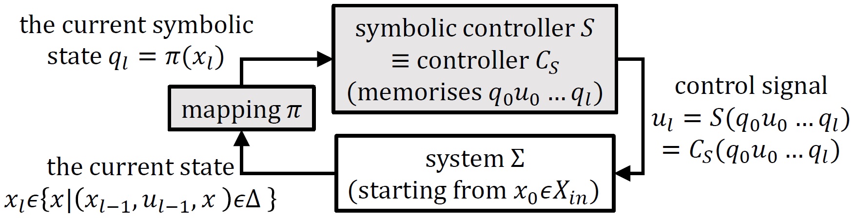
Figure 2: Overview of the symbolic self-triggered control process.

In this section, we reduce the controller synthesis problem for the system $\Sigma_{\tau,\ell,\mu}$ to the synthesis of a symbolic controller for ${{\mathcal{S}}}_{\eta}(\Sigma_{\tau,\ell,\mu})$. The overview of the symbolic control process is depicted in Fig. 2.

By Lemma 1, we can turn any symbolic controller $S:\mathit{FRun}({{\mathcal{S}}}_{\eta}(\Sigma_{\tau,\ell,\mu}))\to{\mathcal{U}}_{\tau,\ell,\mu}$ into a controller $C_{S}:\mathit{FRun}({\mathcal{M}}(\Sigma_{\tau,\ell,\mu}))\to{\mathcal{U}}_{\tau,\ell,\mu}$. More precisely, let $\pi:X\to Q$ be a mapping such that $x\in\mathcal{B}_{\eta}(\pi(x))$. Then, for each run $r=x_{0}u_{1}x_{1}\ldots u_{l}x_{l}\in\mathit{FRun}({\mathcal{M}}(\Sigma_{\tau,\ell,\mu}))$, if $\pi(r)=\pi(x_{0})u_{1}\pi(x_{1})\ldots u_{l}\pi(x_{l})$, then we assign $C_{S}(r)=S(\pi(r))$. By Lemma 1, $\pi(r)$ is a run, and so $C_{S}(r)$ is well defined for any $r\in\mathit{FRun}({\mathcal{M}}(\Sigma_{\tau,\ell,\mu}))$.

Definition 10.

Given a system $\Sigma=(X,X_{\text{in}},U,{{\mathcal{U}}},\xi^{\rightarrow},\xi^{\leftarrow})$, a set $AP$ of atomic propositions, a function $P:X\to{\wp}(AP)$, a $\operatorname{2-LTL}$ path formula $\Phi$, a threshold $\nu\in{\mathbb{R}}_{>0}$, and quantisation parameters $\tau,\ell,\mu,\eta$, the symbolic controller synthesis problem consists in synthesising a symbolic controller $S:\mathit{FRun}({{\mathcal{S}}}_{\eta}(\Sigma_{\tau,\ell,\mu}))\to{\mathcal{U}}_{\tau,\ell,\mu}$ such that

• all finite runs in $\mathit{FRun}({C_{S}}/{{\mathcal{M}}(\Sigma)})$ can be extended to an infinite run in $\mathit{Run}({\mathcal{M}}(\Sigma))$,

• $\sigma\vDash\Phi$ for any $\sigma\in\mathit{Traj}({C_{S}}/{\Sigma})$, and

• $\displaystyle\lim_{h\to\infty}\frac{1}{h}\sum_{i=1}^{h}{{\text{len}}}(u_{i})>\nu$ for any $x_{0}u_{0}\ldots\in\mathit{Run}({C_{S}}/{{\mathcal{M}}(\Sigma)})$.

or determine that such $S$ does not exist.

By Lemma 1, we have the following theorem.

Theorem 1.

If a symbolic controller $S:\mathit{FRun}({{\mathcal{S}}}_{\eta}(\Sigma_{\tau,\ell,\mu}))$ $\to{\mathcal{U}}_{\tau,\ell,\mu}$ solves the problem of Definition 10, then the controller $C_{S}:\mathit{FRun}({\mathcal{M}}(\Sigma_{\tau,\ell,\mu}))\to{\mathcal{U}}_{\tau,\ell,\mu}$ solves the controller synthesis problem of Definition 7.

V Control Algorithm

The overview of the proposed control algorithm is presented in Fig. 3. From the given system $\Sigma$, the signal-length interval $\ell$, and initial quantisation parameters $\eta=\eta_{0},\mu=\mu_{0},\tau=\tau_{0}$, we construct the symbolic model ${{\mathcal{S}}}_{\eta}(\Sigma_{\tau,\ell,\mu})$. Then, we transform the symbolic control problem to a threshold problem of a mean-payoff parity game. If there exists a wining strategy of the controller for the game, the algorithm translates the strategy to a symbolic controller and terminates. Otherwise, the algorithm refines the quantisation parameters (e.g., setting $\eta=\frac{\eta}{2}$, or $\mu=\frac{\mu}{2}$, or $\tau=\frac{\tau}{2}$) and repeats the process. The algorithm terminates without solving the problem when the parameters $\eta,\mu,\tau$ are smaller than some given thresholds.

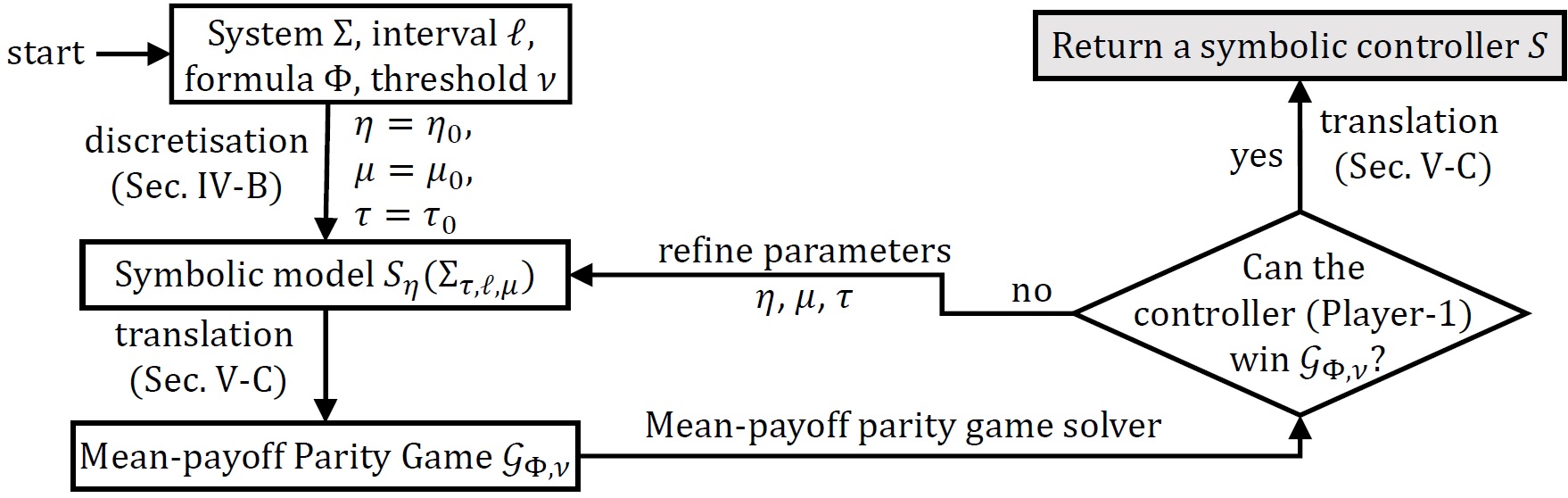
Figure 3: Overview of the proposed control algorithm.

V-A Mean-payoff Parity Game

Let us first start by recalling known results about mean-payoff parity games (MPPGs), which we use for solving the symbolic controller synthesis problem. We invite an interested reader to see [20] for more details about MPPGs.

Definition 11.

A mean-payoff parity game is a tuple $\mathcal{G}=\big{(}G=(V=V_{1}\sqcup V_{2},E,s\colon E\to V,t\colon E\to V),\lambda,c,\nu\big{)}$, where

• $G=(V=V_{1}\sqcup V_{2},E,s\colon E\to V,t\colon E\to V)$ is a directed graph. $V$ is partitioned into two disjoint sets $V_{1}$ and $V_{2}$ of vertices for Player-1 and Player-2, respectively. $E$ is its set of edges. Functions $s$ and $t$ map edges to their sources and targets.

• $\lambda\colon E\to\mathbb{Z}_{\geq 0}$ maps each edge to its payoff.

• $c\colon V\to\mathbb{Z}_{\geq 0}$ maps each vertex to its colour.

• $\nu\in\mathbb{Z}_{\geq 0}$ is a given mean-payoff threshold.

A play on $\mathcal{G}$ is an infinite sequence $\omega=v_{0}e_{0}v_{1}e_{1}\ldots\in(VE)^{\omega}$ such that, for all $i\geq 0$, $s(e_{i})=v_{i}$ and $t(e_{i})=v_{i+1}$. A finite play is a finite sequence in $V(EV)^{*}$ defined in the same way. Let $\mathit{FPlay}$ be the set of all finite plays, and $\mathit{FPlay}_{1}$ and $\mathit{FPlay}_{2}$ be the sets of finite plays ending with a vertex in $V_{1}$ and $V_{2}$, respectively. Both players play the game by selecting strategies. A strategy of Player-$i$ is a partial function $\sigma_{i}\colon\mathit{FPlay}_{i}\rightharpoonup E$ such that $s(\sigma_{i}(v_{0}e_{0}\ldots v_{n}))=v_{n}$, i.e., $\sigma_{i}$ chooses an edge whose source is the ending vertex of the play if such an edge exists, and does not choose any edge otherwise. A play $\omega=v_{0}e_{0}v_{1}e_{1}\ldots$ is consistent with $\sigma_{i}$ if $e_{j}=\sigma_{i}(v_{0}e_{0}\ldots v_{j})$ for all $v_{j}\in V_{i}$. For an initial vertex $v$ and a pair of strategies $\sigma_{1}$ and $\sigma_{2}$ of both players, there exists a unique play, denoted by $\mathit{play}(v,\sigma_{1},\sigma_{2})$, consistent with both $\sigma_{1}$ and $\sigma_{2}$. This play may be finite if a player cannot choose an edge.

For an infinite play $\omega=v_{0}e_{0}v_{1}e_{1}\ldots$, we denote the maximal colour that appears infinitely often in the sequence $c(v_{0})c(v_{1})\ldots$ by $\operatorname{Inf}(\omega)$. Then, the mean-payoff value of the play $\omega$ is $\operatorname{MP}(\omega)=\lim_{n\to\infty}\frac{1}{n}\sum_{i=1}^{n}\lambda(e_{i})$. A vertex $v\in V$ is winning for Player-1 if there exists a strategy $\sigma_{1}$ of Player-1 such that, for any strategy $\sigma_{2}$ of Player-2, $\mathit{play}(v,\sigma_{1},\sigma_{2})$ is infinite, $\operatorname{Inf}(\mathit{play}(v,\sigma_{1},\sigma_{2}))$ is even and $MP(\mathit{play}(v,\sigma_{1},\sigma_{2}))>\nu$. Such a strategy $\sigma_{1}$ is called a winning strategy for Player-1 from the vertex $v$. Then, the threshold problem [21] is to compute the set of winning vertices of Player-1 for a given MPPG.

In [21], the authors propose a pseudo-quasi-polynomial algorithm that solves the threshold problem and computes a winning strategy for Player-1 from each winning state. In Section V-C, we reduce the symbolic control problem to the synthesis of a winning strategy on an MPPG, which can be solved using this algorithm.

V-B Atomic Propositions along Symbolic Transitions

We introduce functions ${\rho_{\exists}},{\rho_{\forall}}:\delta\to{\wp}({\wp}(AP)\times{\wp}(AP))$ to under-approximate the set of atomic propositions that hold along trajectories. This is needed because the information about which states are visited along a trajectory is lost in the discrete model. These functions help recover part of this information, and will be crucial in the problem translation in Section V-C.

For each transition $(q,u,q^{\prime})\in\delta$ in the symbolic model ${{\mathcal{S}}}_{\eta}(\Sigma_{\tau,\ell,\mu})$, we require that for $\Finv\in\left\{\forall,\exists\right\}$

$$\rho_{\Finv}(q,u,q^{\prime})\subseteq \big{\{}(P^{+},P^{-})\in{\wp}(AP)\times{\wp}(AP)\bigm{|}\forall x\in\mathcal{B}_{\eta}(q),$$

$$\forall x^{\prime}\in\mathcal{B}_{\eta}(q^{\prime}),\forall\sigma\in\mathit{FTraj}(\Sigma_{\tau,\ell,\mu},x,(xux^{\prime})),$$ (3)

$$\Finv t\leq{{\text{len}}}(u),P^{+}\subseteq P(\sigma(t))\wedge P^{-}\cap P(\sigma(t))=\emptyset\big{\}}\text{.}$$

The intuition is as follows. If $(P^{+},P^{-})\in\rho_{\forall}(q,u,q^{\prime})$ (resp. $\rho_{\exists}(q,u,q^{\prime})$), then, at all time (resp. at some time) along the transition $(q,u,q^{\prime})$, all $p\in P^{+}$ hold and no $p\in P^{-}$ holds. Then, we can define $\rho_{\Finv}(q,u,q^{\prime})\vDash\varphi$ inductively on the state formula $\varphi$ in a sound way.

For the implementation, we use functions $B^{+},B^{-}:X\times{\mathbb{R}}\to{\wp}(AP)$ such that, for any state $x\in X$ and any radius $r\in{\mathbb{R}}_{>0}$, $B^{+}(x,r)=\{p\in AP\mid\forall x^{\prime}\in\mathcal{B}_{r}(x),x^{\prime}\vDash p\}$ and $B^{-}(x,r)=\{p\in AP\mid\forall x^{\prime}\in\mathcal{B}_{r}(x),x^{\prime}\nvDash p\}$ are the sets of atomic propositions that are satisfied and not satisfied, respectively, at all states in the ball $\mathcal{B}_{r}(x)$.

Assumption 3.

For any state $x\in X$ and any radius $r\in{\mathbb{R}}_{>0}$, the sets $B^{+}(x,r)$ and $B^{-}(x,r)$ can be computed.

Then, we may use the following functions ${\rho_{\exists}}$ and ${\rho_{\forall}}$.

$${\rho_{\exists}}(q,u,q^{\prime})= \big{(}B^{+}(q,\eta)\cup B^{+}(q^{\prime},\eta),B^{-}(q,\eta)\cup B^{-}(q^{\prime},\eta)\big{)}.$$

$${\rho_{\forall}}(q,u,q^{\prime})= \big{(}B^{+}(q,r)\cap B^{+}(q^{\prime},r),B^{-}(q,r)\cap B^{-}(q^{\prime},r)\big{)},$$

$$\text{ where }r=\beta^{\rightarrow}_{u}(q,{{\text{len}}}(u))+\alpha^{\rightarrow}_{u}(q,{{\text{len}}}(u)).$$

By Assumptions 1 and 2, ${\rho_{\exists}}$ and ${\rho_{\forall}}$ satisfy Equation (3).

V-C Problem Translation to Mean-payoff Game

In this section, we present a translation from the symbolic model ${{\mathcal{S}}}_{\eta}(\Sigma_{\tau,\ell,\mu})=(Q,Q_{\text{in}},{\mathcal{U}}_{\tau,\ell,\mu},\delta)$, a path formula $\Phi$, and a threshold $\nu\in{\mathbb{R}}_{\geq 0}$ to an MPPG $\mathcal{G}_{\Phi,\nu}=(G_{\Phi},\lambda_{\Phi},c_{\Phi},\nu)$. The MPPG is played between the controller (as Player-1) and the non-determinism of the system (as Player-2). The parity constraint will force the controller to induce trajectories that satisfy $\Phi$, while the mean-payoff constraint will ensure that the average length of the chosen input signals is above the threshold. The translation is roughly as illustrated in Fig. (4): Player-1 can move from state $q$ to state $(q,u)$ (corresponding to choosing input signal $u$), then Player-2 can choose to go to any $q_{i}$ reachable from $q$ following $u$ (corresponding to a non-deterministic environmental behaviour). The costs on the edges are such that the mean payoff is equal to the average signal length. Finally, the nodes’ colours are defined inductively on $\Phi$.

Figure 4: Translation to a mean-payoff parity game

More precisely, we first define a graph $G_{\Sigma}=(V_{\Sigma}=V_{1}\sqcup V_{2},E_{\Sigma}=E_{1\to 2}\sqcup E_{2\to 1},s,t)$ and a function $\lambda:E\to\mathbb{Z}_{\geq 0}$ as follows, which corresponds to what is shown in Fig. (4):

• $V_{1}=Q$ and $V_{2}=Q\times{\mathcal{U}}_{\tau,\ell,\mu}$,

• $E_{1\to 2}=Q\times{\mathcal{U}}_{\tau,\ell,\mu}$ and $E_{2\to 1}=\big{\{}((q,u),q^{\prime})|(q,u,q^{\prime})\in\delta\big{\}}$,

• $\forall e=(q,u)\in E_{1\to 2}$, $q\xrightarrow{e}(q,u)$ and $\lambda(e)={{\text{len}}}(u)$,

• $\forall e=((q,u),q^{\prime})\in E_{2\to 1}$, $(q,u)\xrightarrow{e}q^{\prime}$ and $\lambda(e)={{\text{len}}}(u)$.

This will form the base of our game $\mathcal{G}_{\Phi,\nu}$, which will roughly consist of multiple copies of $G_{\Sigma}$, labelled with different colours, built inductively from $\Phi$. Technically, we define $\mathcal{G}_{\Phi,\nu}=((Z_{\Phi}\times V_{\Sigma},Z_{\Phi}\times E_{\Sigma},s_{\Phi},t_{\Phi}),\tilde{\lambda},c_{\Phi},\nu)$, where $\tilde{\lambda}(z,e)=\lambda(e)$, $(z,q)\xrightarrow{(z,(q,(q,u)))}(z,(q,u))$, and $(z,(q,u))\xrightarrow{(z,((q,u),q^{\prime}))}(z^{\prime},q^{\prime})$ for some $z^{\prime}\in Z_{\Phi}$. The number of copies $Z_{\Phi}$, the colour function $c_{\Phi}$, and the target copy $z^{\prime}$ are defined inductively.

For the base cases $\Phi=\Diamond\varphi,\Box\varphi,\Diamond\Box\varphi,\Box\Diamond\varphi$, we only present $\Box\Diamond\varphi$, as the other cases are similar. We need two copies $Z_{\Phi}=\{1,2\}$ of $G_{\Phi}$, labelled with colours $c_{\Phi}(z,v)=z$. Finally, $z^{\prime}$ is $2$ if ${\rho_{\exists}}(q,u,q^{\prime})\vDash\varphi$, and $1$ otherwise. The intuition is that we jump to a state in copy $2$ if we can ensure that there is a state satisfying $\varphi$ on the trajectory leading to that state, and jump to a state in copy $1$ otherwise. From there, it is clear that if we can find a strategy that visits states in copy $2$ infinitely often (the winning condition for parity), then we can force the discrete model to output trajectories that satisfy $\Phi$.

For $\Phi\vee\Psi,\Phi\wedge\Psi$, we synchronise parity automata by remembering, for each colour (say in $\mathcal{G}_{\Psi,\nu}$), the max colour (of $\mathcal{G}_{\Phi,\nu}$) seen during the execution since a larger colour has been seen. This allows us to compute the desired $c_{\Phi\vee\Psi}$ and $c_{\Phi\wedge\Psi}$.

Theorem 2.

From a winning strategy $\sigma$ for Player-1 in $\mathcal{G}_{\Phi,\nu}$, one can effectively compute a symbolic controller $C_{\sigma}$ for ${\mathcal{S}}_{\eta}(\Sigma_{\tau,\ell,\mu})$ that solves the symbolic controller synthesis problem of Definition 10.

Proof.

(sketch) $C_{\sigma}$ copies $\sigma$’s choice of input signals. The parity condition ensures that the controlled system satisfies $\Phi$, while the mean-payoff condition ensures that the average signal length is greater than the threshold. ∎

VI Illustrative Example

We consider the following non-deterministic nonholonomic robot system, which is modified version of [3].

$$\dot{x}(t) =v(1+\lambda(t))\cos(\theta(t))$$

$$\dot{y}(t) =v(1+\lambda(t))\sin(\theta(t)) \dot{\theta}(t)=\omega(t)\hbox to0.0pt{,\hss}$$

where $\omega$ is the input signal for the steering angle, $v$ is the speed of the robot, and $\lambda$ is randomly selected from $[-\bar{\lambda},\bar{\lambda}]$ for a given parameter $\bar{\lambda}\in{\mathbb{R}}_{\geq 0}$. Notice in particular how this simple system verifies no stability assumption.

$\xi^{\rightarrow}$ and $\xi^{\leftarrow}$ may be over-approximations of how the physical system behaves. The non-determinism in the system may come from the physical system or its mathematical modelling (e.g., to account for floating-point errors). For the system described above, the non-determinism comes from the physical system, where the velocity of the robot is known only up to some error bound.

Recall that we only consider piecewise-constant input signals in ${\mathcal{U}}_{\tau,\ell,\mu}$ (see Section IV-A). For each signal $\omega$ of length $m\tau$, let $\omega_{0},\omega_{1},\ldots,\omega_{m-1}$ be the constants signals of length $\tau$ such that $\omega_{k}(t)=\omega(k\tau+t)$ for any $t\leq\tau$ and $k\in\{0,...,m-1\}$. Then, we define $\beta^{\rightarrow}_{\omega}$ and $\alpha^{\rightarrow}_{\omega}$ as follows.

$$\beta^{\rightarrow}_{\omega}(d,k\tau+t)=$$

$$\left\{\begin{array}[]{ll}d+2v(1+\bar{\lambda})\sin(\frac{d}{2})(k\tau+t-\displaystyle\sum_{i=0}^{k-1}f_{\omega_{i}}(\tau)-f_{\omega_{k}}(t))&\text{if $d<\pi$}\\ d+2v(1+\bar{\lambda})(k\tau+t-\displaystyle\sum_{i=0}^{k-1}f_{\omega_{i}}(\tau)-f_{\omega_{k}}(t))&\text{otherwise,}\end{array}\right.$$

$$\alpha^{\rightarrow}_{\omega}(d,k\tau+t)=d+v(1+\bar{\lambda})(k\tau+t-\sum_{i=0}^{k-1}f_{\omega_{i}}(\tau)-f_{\omega_{k}}(t)),$$

$$\quad\text{where }f_{\omega}(t)=\left\{\begin{array}[]{ll}\frac{\lfloor\frac{\omega t}{\pi}\rfloor(\pi-2)}{\omega}&\text{if $\omega\neq 0$}\\ 0&\text{otherwise.}\end{array}\right.$$

Functions $\beta^{\leftarrow}_{\omega}$ and $\alpha^{\leftarrow}_{\omega}$ are defined in the same way.

We implement our control algorithm using $v=2.5$, $\bar{\lambda}=0.05$, $X=[-6,6]\times[-6,6]\times[0,2\pi]$, $X_{\text{in}}=\{(0,0,\frac{\pi}{4})\}$, $U=[-\frac{\pi}{2},\frac{\pi}{2}]$, $\eta=\begin{bmatrix}1&1&\frac{\pi}{8}\end{bmatrix}^{\intercal}$, $\mu=\frac{\pi}{2}$, $\tau=\ell_{\text{min}}=0.5$, and $\ell_{\text{max}}=1$. For the control specification, we set the threshold $\nu=0.75$ and $\Phi=\Box\Diamond\varphi$ where $\begin{bmatrix}x&y&\theta\end{bmatrix}^{\intercal}\vDash\varphi\iff x>0\wedge y>0$. In other words, we require the average signal length to be greater than $0.75$ and the robot to always run back to the green region in Fig. 5 after leaving the region.

The program was implemented in Python3.7 and run on a standard laptop computer (Intel i7-7600U 2.80GHz, 12GB memory). The symbolic model contains 3384 states and the mean-payoff game contains 26,400 vertices. To solve the mean-payoff parity game, we combine the algorithm in [21] with the algorithms for energy parity games [22] and mean-payoff games [23] to make it more tractable. All processes took 17 minutes in total. Fig. 5 shows an example of a finite run under the synthesised controller, where the Player-2 (the non-determinism of the system) plays the game by selecting the outgoing edges randomly.

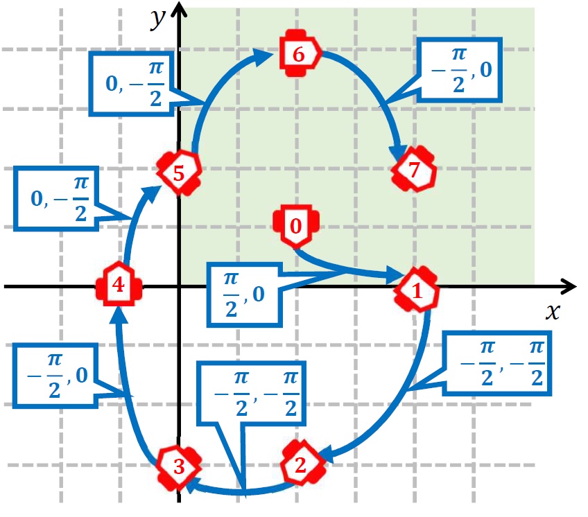
Figure 5: A finite run under the synthesised controller in 7 time steps. The labels of the arrows show the input signals. For example, the arrow from position 0 to 1 represents the signal that assigns $\omega=\frac{\pi}{2}$ for $\tau=0.5$ second, and then assigns $\omega=0$ for another $\tau=0.5$ second.

VII Conclusion and Future Work

In this paper, we proposed a self-triggered control synthesis procedure for non-deterministic continuous-time nonlinear systems without stability assumptions. The two main ingredients of this procedure are 1) discretising the state and input spaces to obtain a discrete symbolic model corresponding to the original continuous system 2) reducing the control synthesis problem to the computation of a winning strategy in a mean-payoff parity game. We illustrated our method on the example of a nonholonomic robot navigating in an arena, under a specification requiring it to repeat some reachability tasks. As a future work, we would like to expand the size of the considered fragment of LTL.

VIII ACKNOWLEDGEMENTS

We thank Prof. Kazumune Hashimoto from Osaka University for his fruitful comments.

References

- [1] W. P. M. H. Heemels, K. H. Johansson, and P. Tabuada, “An introduction to event-triggered and self-triggered control,” in Proc. 51st IEEE Conference on Decision and Control (CDC), 2012, pp. 3270–3285.
- [2] K. Hashimoto, S. Adachi, and D. V. Dimarogonas, “Energy-aware networked control systems under temporal logic specifications,” in Proc. 57th Conference on Decision and Control (CDC), 2018, pp. 132–139.
- [3] C. Santos, F. Espinosa, M. Martinez-Rey, D. Gualda, and C. Losada, “Self-triggered formation control of nonholonomic robots,” Sensors (Basel, Switzerland), vol. 19, no. 12, pp. 132–139, Jun. 2019.
- [4] A. Anta and P. Tabuada, “To sample or not to sample: Self-triggered control for nonlinear systems,” IEEE Transactions on automatic control, vol. 55, no. 9, pp. 2030–2042, 2010.
- [5] K. Hashimoto, A. Saoud, M. Kishida, T. Ushio, and D. V. Dimarogonas, “A symbolic approach to the self-triggered design for networked control systems,” IEEE Control Systems Letters, vol. 3, no. 4, pp. 1050–1055, 2019.
- [6] K. Hashimoto and D. V. Dimarogonas, “Synthesizing communication plans for reachability and safety specifications,” IEEE Transactions on Automatic Control, vol. 65, no. 2, pp. 561–576, 2019.
- [7] E. A. Emerson and C. S. Jutla, “Tree automata, mu-calculus and determinacy,” in Proc. 32nd annual symposium on Foundations of computer science (SFSC’91). Association for Computing Machinery, 1991, pp. 368–377.
- [8] O. Friedmann, M. Lange, and M. Latte, “Satisfiability games for branching-time logics,” Logical Methods in Computer Science, vol. 9, no. 4, 2013.
- [9] M. Luttenberger, P. J. Meyer, and S. Sickert, “Practical synthesis of reactive systems from ltl specifications via parity games,” Acta Informatica, vol. 57, pp. 3–36, 2019.
- [10] A. Ehrenfeucht and J. Mycielski, “Positional strategies for mean-payoff game,” International journal of game theory, vol. 8, no. 2, pp. 109–113, 1979.
- [11] S. Pruekprasert, T. Ushio, and T. Kanazawa, “Quantitative supervisory control game for discrete event systems,” IEEE Transactions on Automatic Control, vol. 61, no. 10, pp. 2987–3000, 2016.
- [12] Y. Ji, X. Yin, and S. Lafortune, “Mean payoff supervisory control under partial observation,” in Proc. 57th IEEE Conference on Decision and Control (CDC), 2018, pp. 3981–3987.
- [13] K. Kido, S. Sedwards, and I. Hasuo, “Bounding errors due to switching delays in incrementally stable switched systems,” IFAC-PapersOnLine, vol. 51, no. 16, pp. 247–252, 2018.
- [14] M. Zamani, P. Mohajerin Esfahani, R. Majumdar, A. Abate, and J. Lygeros, “Symbolic control of stochastic systems via approximately bisimilar finite abstractions,” IEEE Transactions on Automatic Control, vol. 59, no. 12, pp. 3135–3150, 2014.
- [15] E. Macoveiciuc and G. Reissig, “Memory efficient symbolic solution of quantitative reach-avoid problems,” in Proc. American Control Conference (ACC), 2019, pp. 1671–1677.
- [16] M. Zamani, G. Pola, M. Mazo, and P. Tabuada, “Symbolic models for nonlinear control systems without stability assumptions,” IEEE Transactions on Automatic Control, vol. 57, no. 7, pp. 1804–1809, 2012.
- [17] D. Angeli and E. D. Sontag, “Forward completeness, unboundedness observability, and their lyapunov characterizations,” Systems and Control Letters, vol. 38, no. 4, pp. 209–217, 1999.
- [18] D. Angeli, “A lyapunov approach to incremental stability properties,” IEEE Transactions on Automatic Control, vol. 47, no. 3, pp. 410–421, 2002.
- [19] G. Pola and P. Tabuada, “Symbolic models for nonlinear control systems: Alternating approximate bisimulations,” SIAM Journal on Control and Optimization, vol. 48, no. 2, pp. 719–733, 2009.
- [20] K. Chaterjee, T. A. Henzinger, and M. Jurdzinski, “Mean-payoff parity games,” in Proc. 20th Annual IEEE Symposium on Logic in Computer Science (LICS’ 05). IEEE, 2005.
- [21] L. Daviaud, M. Jurdziński, and R. Lazić, “A pseudo-quasi-polynomial algorithm for mean-payoff parity games,” in Proc. 33rd Annual ACM/IEEE Symposium on Logic in Computer Science, 2018, pp. 325–334.
- [22] K. Chatterjee and L. Doyen, “Energy parity games,” Theoretical Computer Science, vol. 458, pp. 49–60, 2012.
- [23] L. Brim, J. Chaloupka, L. Doyen, R. Gentilini, and J.-F. Raskin, “Faster algorithms for mean-payoff games,” Formal Methods in System Design, vol. 38, no. 2, pp. 97–118, 2010.