On Dark Matter Explanations of the Gamma-Ray Excesses from the Galactic Center and M31

Abstract

The presence of an excess $\gamma$-ray signal toward the Galactic center (GC) has now been well established, and is known as the GC excess. Leading explanations for the signal include mis-modeling of the Galactic diffuse emission along the line of sight, an unresolved population of millisecond pulsars, and/or the annihilation of dark matter (DM). Recently, evidence for another excess $\gamma$-ray signal has been reported toward the outer halo of M31. In this work we interpret the excess signals from both the GC and outer halo of M31 in the framework of DM annihilation, and show that the two spectra are consistent with a DM origin once $J$-factors are taken into account. We further compare the excesses to models of DM annihilation, and determine the corresponding best-fit parameters. We find good fits to the spectrum both in two body and four body annihilation modes.

I Introduction

There is now overwhelming evidence that most of the matter in the Universe is composed of dark matter (DM)  Riess et al. (1998); Perlmutter et al. (1999); Clowe et al. (2006); Hinshaw et al. (2013); Ade et al. (2016); Eisenstein et al. (2005); Anderson et al. (2014); Tanabashi et al. (2018); Peacock et al. (2001). However, despite much experimental effort for many decades now, the nature of DM still remains elusive. Determining the characteristics of DM is one of the most important outstanding problems in particle physics.

One of the most promising approaches for detecting DM is indirect detection. DM particles can annihilate or decay to Standard Model (SM) particles, which can be detected in astrophysical searches. In particular, annihilation or decay into photons gives a striking signal, since their direction of arrival is correlated with their annihilation location, and because photons can travel over large distances.

Simulations predict that the highest DM density should be near the Galactic center (GC), though models differ on the exact profile shape. Since the annihilation signal goes as the square of the density, the GC is thus expected to be one of the brightest sources of $\gamma$-rays from DM annihilation, and this makes it is an important target for indirect searches.

It has now been well established that there exists an excess of $\gamma$-rays toward the GC (as compared to the expected background) Goodenough and Hooper (2009); Hooper and Goodenough (2011); Hooper and Linden (2011); Abazajian and Kaplinghat (2012); Hooper and Slatyer (2013); Gordon and Macías (2013); Huang et al. (2013); Daylan et al. (2016); Abazajian et al. (2014); Ajello et al. (2016); Zhou et al. (2015); Calore et al. (2015a); Abazajian et al. (2015); Calore et al. (2015b); Carlson et al. (2016); Das and Dasgupta (2017). Intriguingly, the signal is found to be broadly consistent with having a DM origin, in regards to the energy spectrum and morphology. However, there are other plausible interpretations of the excess, including mis-modeling of the foreground emission from the Milky Way (MW), and an un-resolved population of point sources, such as millisecond pulsars List et al. (2020); Fragione et al. (2019, 2018). These other possibilities make it very difficult to extract a DM signal with a high degree of confidence.

Determining whether or not the GC excess does in fact have a DM origin (at least in part) will likely require complementarity with other targets, as well as other search methods (e.g. direct detection). For $\gamma$-ray searches, the MW’s dwarf spheroidal (dSph) satellite galaxies offer another promising target, as they are expected to be dominated by DM, with very little astrophysical background. However, thus far there has been no global signal detected, a result that is in tension with the DM interpretation of the GC excess  Ackermann et al. (2015); Albert et al. (2017). However, it is important to note that the limits from the dSphs are subject to systematic uncertainties relating to their DM content, and this prohibits their ability to robustly constrain the GC excess Ando et al. (2020); Bonnivard et al. (2015); Klop et al. (2017).

Looking beyond the MW, the Andromeda galaxy (also known as M31) is the closest large spiral galaxy to us and is predicted to be the brightest extragalactic source of DM annihilation Lisanti et al. (2018a, b). Recently, observations towards M31’s outer halo reported evidence for an excess signal, with a peak in the $\gamma$-ray spectrum at an energy similar to the GC excess Karwin et al. (2019). Moreover, the analysis is based on the outer regions of M31 where backgrounds from standard astrophysical emission are less dominant. It is thus plausible that both these signals result from DM annihilation.

In this work we perform a simultaneous analysis of the GC and M31 to determine if these two excesses are consistent with having a DM origin. We first examine the two spectra and see if they are consistent with each other once $J$-factors are taken into account. This turns out to be the case; furthermore, the required scaling turns out to be within the allowed range from a recent analysis of the M31 $J$-factor Karwin et al. (2020).

We then compare these spectra to various models of DM annihilation, We first consider 2-body final states, such as DM annihilating to bottoms and taus. It is also interesting to consider four-body final states, which are motivated in models where DM which is coupled to the SM through pseudoscalar mediators Karwin et al. (2017); Escudero et al. (2017); Abdullah et al. (2014); Rajaraman et al. (2015) (such models avoid direct detection constraints). We therefore consider a few motivated examples of annihilation to four final-state particles. As we shall show, both two-body annihilations and four-body annihilations can produce good fits to the observed spectra.

The paper is organized as follows. In section II we review the observational data leading to the GC excess, and the more recent signal towards the outer halo of M31. We also review the current bounds on the $J$-factors of the two signal regions. In the following section, Section III, we compare the M31 and GC spectra and examine whether they are consistent with the allowed $J$-factors. We then, in Section IV, consider the spectra from specific DM models, for example, annihilation to b-quarks, and find the best fit to the observations. We end with a summary of our results. In Appendix A, we present results for other two-body and four-body annihilation channels, along with a table summarizing all our results.

II Review of GC and M31 Observations

II.1 GC

For the GC excess we use data from Ref. Ajello et al. (2016). Here we summarize a few main aspects of the analysis. The observations are based on approximately 5.2 years of Fermi-LAT data, with energies between 1–100 GeV, in 20 logarithmically spaced energy bins.

A majority of the diffuse emission in the Galaxy is due to the interaction of cosmic rays (CRs) with the interstellar gas and radiation fields. Indeed, the emission toward the GC is dominated by standard astrophysical processes, and the GC excess only amounts to a small fraction of the total emission. To quantify the uncertainty in the foreground/background emission, Ref. Ajello et al. (2016) employs the CR propagation code GALPROP Moskalenko and Strong (1998, 2000); Strong and Moskalenko (1998); Strong et al. (2000); Ptuskin et al. (2006); Strong et al. (2007); Vladimirov et al. (2011); Jóhannesson et al. (2016, 2018); Porter et al. (2017); Génolini et al. (2018) to build four different interstellar emission models (IEMs), corresponding to two main systematic variations.

First, Galactic CRs are thought to be accelerated primarily from supernova remnants (SNRs) via diffusive shock acceleration (see Ref. Ajello et al. (2016) and references therein). However, the distribution of SNRs is not well determined due to the observational bias and the limited lifetime of their shells, and so other tracers are often employed. Ref. Ajello et al. (2016) uses two possible tracers, namely, the distribution of OB stars, which are progenitors of supernovae, and pulsars, which are the end states of supernovae.

The second main variation comes from the tuning of the IEMs to the $\gamma$-ray data. This was done outside of the signal region, working from the outer Galaxy inward, with two variations in the fit. In the intensity-scaled variation, only the normalizations of the IEM components were left free to vary. In the index-scaled variation, additional degrees of freedom were given to the gas-related components interior to the Solar circle by also freely scaling the spectral index.

Combining the variations in the CR density and the tuning procedure gives four possible IEMs which quantify the uncertainty in the foreground/background emission. We shall denote these four IEMs as (a) OB Stars, index-scaled (b) OB Stars, intensity-scaled (c) Pulsars, index-scaled; and (d) Pulsars, intensity-scaled. Figure 1 shows the spectra for the GC excess, corresponding to the four IEMs. Note that the intensity-scaled models have a high energy tail which is not present in the index-scaled models.

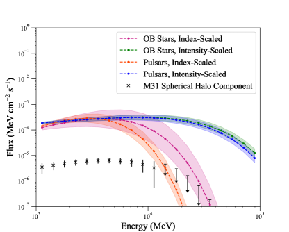
Figure 1: The colored dashed lines show the spectra of the GC excess for different IEMs, based on Ref. Ajello et al. (2016). The bands show the 1$\sigma$ uncertainty. Black points show the spectrum for M31’s spherical halo component, based on Ref. Karwin et al. (2019).

II.2 M31

For the M31 analysis we follow Ref. Karwin et al. (2019). The analysis employs 7.6 years of Fermi-LAT data, with energies between 1–100 GeV, in 20 logarithmically spaced energy bins. Similar to the GC, the foreground emission from the MW is the dominant component when looking towards M31’s outer halo, and Ref. Karwin et al. (2019) again used GALPROP to build specialized IEMs to characterize the emission.

Evidence for an excess signal was found, having a radial extension of $\sim 120-200$ kpc from the center of M31. To characterize the excess, three additional signal components were added to the model (i.e. in addition to the IEM). For the inner galaxy a $0.4^{\circ}$ disk was used, consistent with what has previously been reported Abdo et al. (2010); Pshirkov et al. (2016); Ackermann et al. (2017). A second concentric ring was also added, extending from $0.4^{\circ}$ to $8.5^{\circ}$ (corresponding to a projected radius of $\sim$120 kpc); this is referred to as the spherical halo component. Finally, a third concentric ring was added, extending from $8.5^{\circ}$ and covering the remaining extent of the field (corresponding to a projected radius of $\sim$200 kpc); this is referred to as the far outer halo component.

Here, we only use data from the spherical halo region, and the corresponding spectrum is shown in Figure 1. The inner galaxy is problematic for two reasons. First, it is difficult to disentangle a possible DM signal from standard astrophysical emission. Secondly, there still remains a high systematic uncertainty to the actual $\gamma$-ray signal that is detected Karwin et al. (2019, 2020). This is due to an uncertainty in the underlying H I gas maps that are used for the Milky Way (MW) foreground. We also ignore the far outer halo region because it begins to approach the MW disk toward the top of the field, which significantly complicates the analysis. If the excess $\gamma$-ray emission observed toward M31’s outer halo does in fact have a physical association with the M31 system, then it is particularly important to establish this in the spherical halo region Karwin et al. (2020).

II.3 J-factors

The greatest uncertainty for the DM interpretation of M31’s outer halo comes from the $J$-factor. This is covered in extensive detail in Ref. Karwin et al. (2020). Here, we use results from that study to quantify the full uncertainty range, and below we summarize the key points.

The $J$-factor characterizes the spatial distribution of the DM, and is given by the integral of the mass density squared, over the line of sight. When describing the DM distribution as an ensemble of disjoint DM halos, the $J$-factor is:

$$J=\sum_{i}\int_{\Delta\Omega}d\Omega\int_{\text{LoS}}ds\rho_{i}^{2}(\mathbf{r}_{i}(s,\mathbf{n})),$$ (1)

summed over all halos in the line of sight (LoS), where $\rho_{i}(\mathbf{r})$ is the density distribution of halo $i$, and $\mathbf{r}_{i}(s,\mathbf{n})$ is the position within that halo at LoS direction $\mathbf{n}$ and LoS distance $s$.

$J$-factors determined from these spherically-averaged profiles are an underestimate of the total $J$-factor because of the effect of the non-spherical structure. This underestimate is typically encoded with a boost factor. The substructure component is very important for indirect detection, as it enhances the overall signal, since the predicted $\gamma$-ray flux scales as the mass density squared. This is especially true for MW-sized halos and toward the outer regions.

The main uncertainties in the boost factor include the minimum subhalo mass, the subhalo mass function, the concentration-mass relation, the distribution of the subhalos in the main halo, the mass distribution of the subhalos themselves, and the number of substructure levels. In Ref. Karwin et al. (2020) these physical parameters are varied within physically motivated ranges (as representative of the current uncertainty found in the literature) in order to quantify the uncertainty in the substructure boost. Additionally, there is also an uncertainty in the halo geometry, which is quantified by calculating $J$-factors for the different experimental estimates found in the literature.

In addition to the substructure and halo geometry, another primary driver of the $J$-factor uncertainty for obervations toward M31’s outer halo is the contribution to the signal from the MW’s DM halo along the line of sight, which is also accounted for in Ref. Karwin et al. (2020). Including all these uncertainties, the $J$-factor integrated over the spherical halo region, (which we will henceforth denote as $J_{M31}$) is found to range from $(2.0-31.1)\times 10^{20}\mathrm{\ GeV^{2}\ cm^{-5}}$, with a geometric mean of $7.9\times 10^{20}\mathrm{\ GeV^{2}\ cm^{-5}}$. We emphasize that this range accounts for the contribution from the MW’s halo along the line of sight.

For the GC we use the $J$-factor from Ref. Ajello et al. (2016) that was used to extract the excess signal (which is consistent with the data that we use in this analysis). This corresponds to an NFW density profile with a slope $\gamma=1$, a scale radius $r_{\mathrm{s}}=20\ \mathrm{kpc}$, and local DM density $\rho_{\odot}=0.3\ \mathrm{GeV\ cm^{-3}}$. The $J$-factor integrated over the $15^{\circ}\times 15^{\circ}$ GC region (which we will henceforth denote as $J_{GC}$) has a value of $2.2\times 10^{22}\mathrm{\ GeV^{2}\ cm^{-5}}$. We note that there is an uncertainty in the GC $J$-factor due to the value of the local DM density, as well as the other parameters in the density profile. However, in this work we consider just the uncertainty in the M31 $J$-factor, since it is dominant.

As described in more detail in the next section, a particularly important quantity in our analysis will be the ratio of the $J$-factors:

$$J_{r}\equiv J_{GC}/J_{M31}$$ (2)

For the values of $J_{M31}$ between $(2.0-31.1)\times 10^{20}\mathrm{\ GeV^{2}\ cm^{-5}}$, and $J_{GC}=2.2\times 10^{22}\mathrm{\ GeV^{2}\ cm^{-5}}$ we find that $J_{r}$ lies between $J_{r,low}=7.07$ and $J_{r,high}=110.0$. Using the geometric mean of $J_{M31}=7.9\times 10^{20}\mathrm{\ GeV^{2}\ cm^{-5}}$, we define $J_{r,mid}=28.17$.

III Spectral Comparison of the GC and M31 Excesses

III.1 Best-fit J-factor ratios

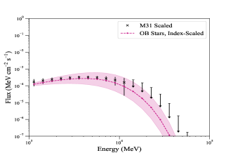
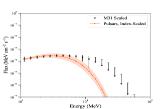
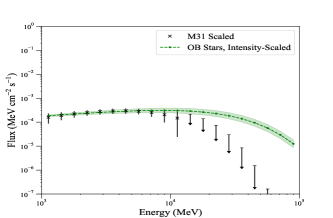
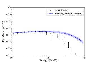
Figure 2: Comparison of GC spectra (colored bands) to scaled M31 spectra (black data points). The bands and error bars give the $1\sigma$ statistical error. The top two panels show the index-scaled IEMs, and the bottom two panels show the intensity-scaled IEMs. In each case the M31 data is scaled by the appropriate $J$-factor for the IEM.

The flux observed from M31 is much lower than that of the GC excess. If the excesses are indeed from an underlying DM model, then the underlying cross-section for DM annihilation to photons should be the same. The difference in the spectra would then be attributable mostly to the ratio between $J_{M31}$ and $J_{GC}$. We note, however, that there may be some differences that arise from secondary emission, which depends on the particular astrophysical backgrounds in each respective targets (i.e. the gas and interstellar radiation fields) Cirelli et al. (2013). For simplicity these effects are not considered in this analysis.

To test the agreement between the two spectra we multiply the M31 data by a scaling factor. This factor is then the ratio $J_{r}$. Since the four GC background models yield significantly different spectra, we fit the scaling factor independently for each of them.

The best-fit scaling factor is determined using a $\chi^{2}$ fit. We account for upper limits (ULs) in the data by including an error function in the $\chi^{2}$ definition  Lyu et al. (2016); Isobe et al. (1986); Karwin et al. (2020)

$$\chi^{2}=\sum_{i=1}^{m}w_{i}^{2}-2\sum_{i=m+1}^{20}\mathrm{ln}\frac{1+\mathrm{erf}(w_{i}/\sqrt{2})}{2}$$ (3)

where

$$w_{i}={(\frac{y_{i}}{z_{i}}-J)\over\sigma_{i}^{r}}$$ (4)

and

$$\mathrm{erf}(z)=\tfrac{2}{\sqrt{\pi}}\int_{0}^{z}e^{-t^{2}}\,\mathrm{d}t$$ (5)

The first term on the right-hand side of Eq. (3) is the classic definition of $\chi^{2}$, and the second term introduces the error function to quantify the fitting of ULs. The number of good data points is given by $m$, and the sum is over the 20 energy bins. Here $y_{i}$ is the flux from the GC and $z_{i}$ is the flux from M31, for the ith energy bin.

The error on the flux ratio $J_{r}$ is taken to be

$$\sigma_{i}^{r}=\frac{\sigma_{i}^{y}}{z_{i}}$$ (6)

where we use just the statistical error on the GC data, which we assume to be symmetric. This allows for a reasonable spectral comparison, and is further justified by the fact the uncertainty in the GC excess is dominated by the systematics. We note that in general a more sophisticated treatment of the errors may be appropriate (e.g.  Lyu et al. (2016); Karwin et al. (2020)). However, we have tested different prescriptions for handling the error and in all cases we find that the results are qualitatively consistent.

We minimize the $\chi^{2}$ with respect to $J$, and identify the minimum with the optimized rescaling factor. The third column of Table 1 shows the best-fit results for each IEM. We note that the best-fit $J$-factor ratios are well within the bounds from section II.3. There is a preference for smaller values of $J_{r}\sim 40$, corresponding to larger values of $J_{M31}$. We will refer to these as the model-independent $J_{r}$ values (as these are found without reference to a specific DM annihilation model).

IEM	$J_{r}$
Pulsars, intensity-scaled	$48.96\pm 2.31$
Pulsars, index-scaled	$36.63\pm 3.37$
OB Stars, intensity-scaled	$48.76\pm 2.22$
OB Stars, index-scaled	$41.24\pm 5.75$

Table 1: $J$-factor ratio for each IEM.

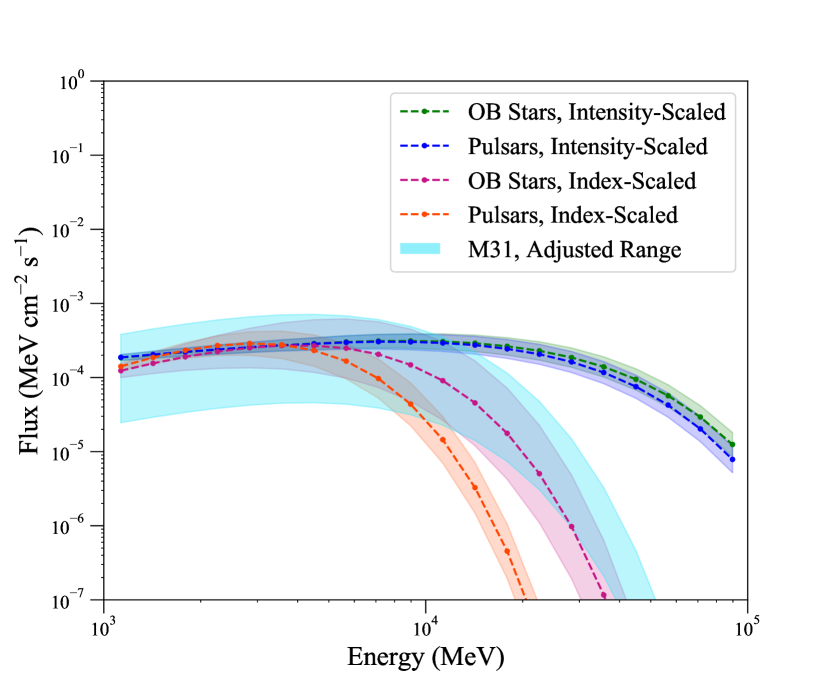
Figure 3: The blue band shows the range of M31 flux values scaled up by a $J$-factor ratio between 7.7 and 110. Dashed lines show the four different GC IEMs with one sigma error bands.

III.2 Spectral Comparisons

We further examine the agreement between the M31 spectrum and the GC excess by scaling the M31 data by the best-fit $J$-ratio found above, and comparing the two spectral shapes. These comparisons are shown in Fig. 2. The top panel shows the rescaled M31 data compared to the GC excess for the index-scaled IEMs. As can be seen, the spectra show excellent agreement.

The bottom panel shows the intensity-scaled IEMs. As can be seen, there is a strong tension between the GC and M31 spectra at high energy (above $\sim$10 GeV). This is due to the existence of the so-called ”high-energy tail” in the intensity-scaled IEMs. The nature of the high-energy tail of the GC excess has been investigated in numerous studies (e.g. Ajello et al. (2016); Calore et al. (2015); Horiuchi et al. (2016); Linden et al. (2016)). It remains uncertain whether this feature is a true property of the signal or if it is due to mis-modeling of the background. When comparing the GC excess to the M31 excess, it is important to note that the two signals are extracted from very different regions of the galaxy, and thus they may not be directly comparable. In particular, this is the case when considering secondary emission, which depends on the astrophysical backgrounds. With that said, the M31 data does not possess a high-energy tail, and so seems to be in strong tension with those models. Indeed, this would be in general agreement with previous studies which have found that the high-energy tail is not very compatible with having a pure DM explanation Horiuchi et al. (2016); Linden et al. (2016).

One can also examine whether a different choice of $J$-factor could ameliorate the tension at high energies between the M31 excess and the intensity scaled GC excesses. To examine this, we find the range of possibilities for the M31 flux, by rescaling it by the maximum and minimum $J$-factors allowed from Ref. Karwin et al. (2020). Figure 3 shows the scaled M31 data compared to the GC excess for the four IEMs. As can be seen, the M31 data shows good agreement with the index-scaled IEMs, whereas there is still tension with the intensity-scaled IEMs.

IV Dark Matter Models

In this section we perform a DM fit simultaneously to both signals. We will take a model where DM is a real scalar field $\chi$ of mass $m_{\chi}$, and consider various possibilities for the dominant annihilation process; specifically, we will consider both two-body and four-body final states. For the standard WIMP models the DM spectra were generated using PPPC  Cirelli et al. (2011). For the four-body annihilations the spectra were produced using FeynRules Christensen and Duhr (2009) and MadGraph Alwall et al. (2014), and showered with Pythia 8 Sjostrand et al. (2008). The photons were binned in 20 logarithmically-spaced bins from 1$-$100 GeV, just as for the GC and M31 data.

The predicted $\gamma$-ray flux from DM annihilation is given by

$$\left.E^{2}\frac{d\Phi}{dE}\right|_{GC}={\cal N}_{GC}(E^{2}\frac{dn}{dE})$$ (7)

$$\left.E^{2}\frac{d\Phi}{dE}\right|_{M31}=\frac{{\cal N}_{GC}}{J_{r}}(E^{2}\frac{dn}{dE})$$ (8)

Here

$${\cal N}_{GC}=J_{GC}\frac{\langle\sigma v\rangle}{4\pi\eta m_{\chi}^{2}}$$ (9)

where $\langle\sigma v\rangle$ is the velocity averaged cross section, $\eta$ is 2 (4) for conjugate (non-self conjugate) DM, $m_{\chi}$ is the DM mass, and dn/dE is the number of $\gamma$-ray photons per annihilation.

We perform a $\chi^{2}$ fit as in Eqs. 3-5. The main difference is the definition of $w_{i}$. This quantity is defined separately for the GC and M31. For the GC:

$$w_{i}={y_{i}-NE^{2}{dn\over de}\over\sigma^{y}_{i}}$$ (10)

where $\sigma^{y}_{i}$ is the 1-sigma error on the GC flux and $y_{i}$ is the best fit value of the GC flux for a given IEM. Similarly for M31 we have

$$x_{i}={z_{i}-J^{-1}NE^{2}{dn\over de}\over\sigma^{z}_{i}}$$ (11)

where the error $\sigma^{z}_{i}$ is the 1-sigma error on the M31 flux and $z_{i}$ is the best fit value of the M31 flux.

Finally, we define the total chi-squared as

$$\chi^{2}_{tot}=\chi_{GC}^{2}+\chi_{M31}^{2}$$ (12)

We marginalize over $N$ in order to minimize this quantity with respect to $J_{\mathrm{r}}$ and $m_{\chi}$. This is done separately for each GC IEM.

Figure 4 shows the results for the two-body annihilation to bottom quarks with the OB Stars, index-scaled IEM. The color scale indicates the value of $\Delta\chi^{2}$. The best-fit is shown with a red point, and also overlaid are the 1$\sigma$, 2$\sigma$, and 3$\sigma$ confidence contours, corresponding to $\Delta\chi^{2}=2.30,4.61$ and $9.21$, respectively. For comparison, we also show the model-dependent $J_{r}$ value from Table 1 and $J_{r,low},J_{r,mid}$ from Section  II. As can be seen, the $J_{r}$ corresponding to the DM fit is in good agreement with the range found in Ref. Karwin et al. (2019). In Figure  5 we show the corresponding best-fit DM spectrum compared to the GC and scaled M31 data.

We have also extended our analysis to other possible annihilation modes; these results are presented in the Appendix. Specifically, we first considered other two-body annihilations where the DM annihilates to two tau leptons, and the case where the DM annihilates to two light quarks, which we take to be down quarks for concreteness. Figure  6 shows the results for these annihilation channels.

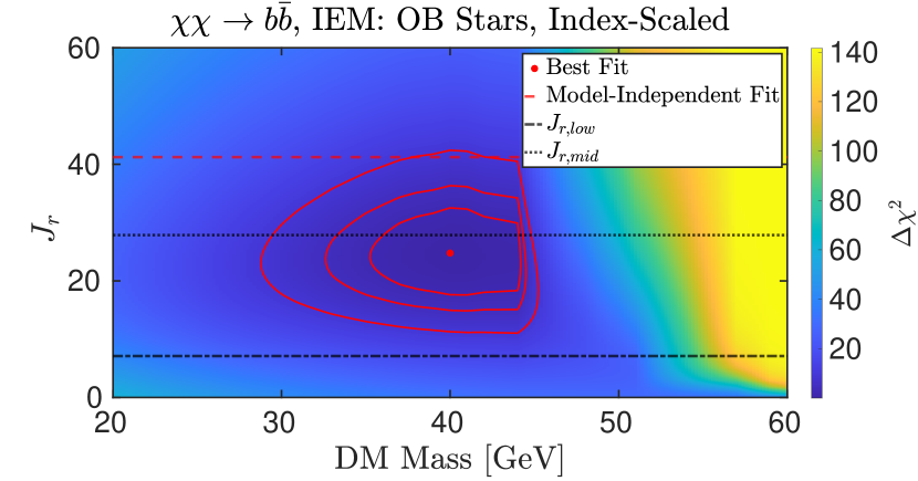
Figure 4: $\Delta\chi^{2}$ for $\chi\chi\rightarrow b\bar{b}$ , for the OB-Stars index-scaled IEM. The red dot indicates the best fit point, and the contours are 1,2, and 3 $\sigma$ contours. The dashed red line shows the model independent $J_{r}$ value. Dash-dotted and dotted black lines show high and mean values of $J_{r}$ from section II.3.

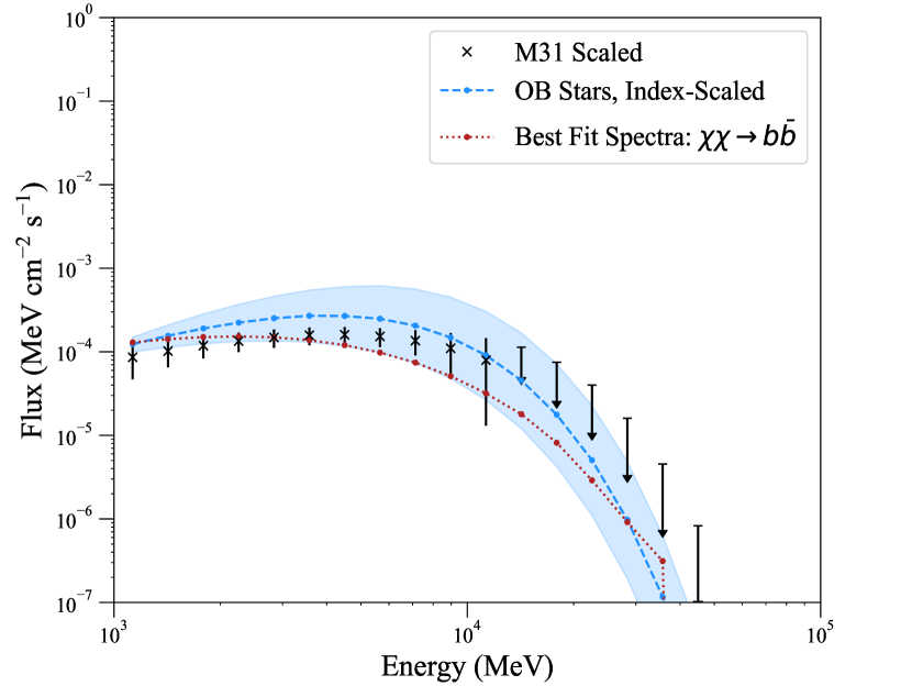
Figure 5: Dashed lines show the GC excess with the OB Stars, index IEM. Black points show the M31 flux data scaled up by the appropriate ratio $J_{r}$ taken from Table 2. The dotted line shows the corresponding best-fit model spectra for $\chi\chi\rightarrow b\bar{b}$.

As mentioned above, direct detection and collider searches significantly constrain DM couplings. This has motivated the study of models where the DM is coupled to the SM quarks through a pseudoscalar mediator Karwin et al. (2017); Escudero et al. (2017); Abdullah et al. (2014); Rajaraman et al. (2015). For example, one can consider a model with a mediator $\phi$ and the interactions

$${\cal L}_{int}=\chi^{2}\phi^{2}+\phi\overline{b}b$$ (13)

In this model, DM primarily annihilates to four b-quarks. The precise annihilation mode depends on the coupling, for example if the mediator coupled as $\phi\overline{d}d$, there would be a annihilation to four d quarks. Generically we get a four-body annihilation.

Results for some possible 4-body final states are shown in Figure  7. We note that the best fit DM mass increases for the four body annihilation mode; this is expected because each quark has less energy.

The corresponding best-fit parameters for all models are summarized in Table  2.

V Conclusion

The GC excess, an excess of $\gamma$-ray photons from the GC, has been a long-standing potential signal of DM annihilation. However, the large astrophysical background and the potential existence of new sources makes it difficult to make definitive statements about the origin of this excess. On the other hand, the M31 excess is from a region where astrophysical backgrounds (not associated with the conventional interstellar emission from the MW foreground) are not expected to be large, and hence lends credence to the possibility that the excess is indeed associated with DM annihilation, rather than an unknown astrophysical background.

We have further examined these two excesses, to see if their magnitudes and spectral shapes are consistent with DM annihilation. The two signals are expected to be related by the ratio of the two $J$-factors. The recent analysis of the M31 $J$-factor allows us to check this relation, and we have found that indeed the excesses are consistent with the determined $J$-factors. The spectral shapes for the index-scaled IEMs are also in very good agreement. On the other hand, there is tension with the intensity-scaled IEMs due to the so-called high-energy tail.

We also fit the excesses to a number of DM models, where the DM annihilates to either two or four SM particles. We found that excellent fits can be achieved both in two-body and four-body annihilations, as can be seen in the Appendix.

In summary, we have found that the M31 excess and the GC excess are mutually consistent with a dark matter origin. The DM models prefer a somewhat higher value for the M31 $J$-factor, and prefer a particular IEM (the index-scaled models) for the GC. Currently, several DM models are consistent with the excesses.

Future prospects to confirm the excess toward the outer halo of M31, and to better understand its nature, will crucially rely on improvements in modeling the interstellar emission towards M31. For the GC, the excess has been under investigation for many years now, and further improvements in the IEM will continue to play a significant role in better understanding the nature of the signal. Additionally, working towards a better understanding of the possible point-like nature of the excess will be key. Improved sensitivity from other indirect detection constraints will also continue to play an important role in DM interpretations of the two signals, and likewise for constraints from direct detection. Further analysis of these complementary signals would be extremely interesting, and could shed light on the nature of DM.

Appendix A: Other Annihilation Channels

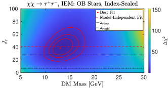
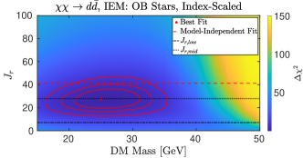
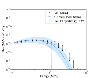
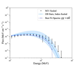
Figure 6: The left panels are similar to Figures 4 and 5 for $\chi\chi\rightarrow\tau\bar{\tau}$, and the right panels are similar to Figures 4 and 5 for $\chi\chi\rightarrow d\bar{d}$

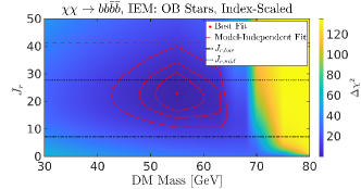
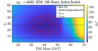
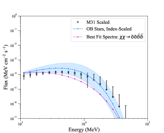
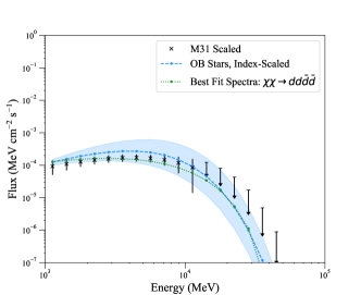
Figure 7: Similar to Fig  6, but for $\chi\chi\rightarrow bb\bar{b}\bar{b}$ and $\chi\chi\rightarrow dd\bar{d}\bar{d}$ respectively.

DM Model	IEM	$m_{\chi}$ [GeV]	${\cal{N}}_{GC}\times 10^{8}$ [cm-2 s-1]	$J_{r}$	$\chi^{2}_{red}$
$b\bar{b}$	Pulsars, intensity-scaled	$57_{-2.1}^{1.3}$	$2.6_{-0.14}^{+0.14}$	$45.9_{-6.9}^{+8.1}$	2.00
	Pulsars, index-scaled	$22_{-0.9}^{+1.9}$	$3.9_{-0.31}^{+0.31}$	$25.7_{-4.8}^{+6.7}$	1.72
	OB Stars, intensity-scaled	$57_{-1.7}^{+1.3}$	$2.7_{-0.16}^{+0.16}$	$45.9_{-6.9}^{+8.0}$	2.4
	OB Stars, index-scaled	$40_{-4.7}^{+4.1}$	$2.1_{-0.10}^{+0.10}$	$24.8_{-7.2}^{+7.8}$	1.01
$d\bar{d}$	Pulsars, intensity-scaled	$43_{-4.9}^{+3.7}$	$3.6_{-0.16}^{+0.16}$	$51.4_{-7.2}^{+9.8}$	1.43
	Pulsars, index-scaled	$17_{-1.3}^{+1.3}$	$5.0_{-0.24}^{+0.24}$	$29.4_{-5.4}^{+6.5}$	0.99
	OB Stars, intensity-scaled	$45_{-5.5}^{+3.1}$	$3.6_{-0.17}^{+0.17}$	$53.2_{-7.7}^{+9.9}$	1.72
	OB Stars, index-scaled	$25_{-4.1}^{+6.1}$	$3.3_{-0.01}^{+0.01}$	$27.5_{-8.0}^{+8.3}$	0.81
$bb\bar{b}\bar{b}$	Pulsars, intensity-scaled	$81_{-3.0}^{+0.3}$	$1.76_{-0.11}^{+0.11}$	$42.2_{-5.8}^{8.4}$	2.40
	Pulsars, index-scaled	$36_{-3.5}^{+1.1}$	$2.4_{-0.19}^{+0.19}$	$24.8_{-5.1}^{+5.9}$	1.92
	OB Stars, intensity-scaled	$81_{-2.5}^{+0.3}$	$1.8_{-0.12}^{+0.12}$	$42.2_{-5.7}^{+8.4}$	2.85
	OB Stars, index-scaled	$55_{-4.1}^{+4.9}$	$1.4_{0.01}^{+0.01}$	$22.9_{-6.3}^{+7.6}$	1.19
$dd\bar{d}\bar{d}$	Pulsars, intensity-scaled	$67_{-6.7}^{+3.9}$	$2.2_{-0.1}^{+0.1}$	$50.5_{-7.5}^{+9.1}$	1.57
	Pulsars, index-scaled	$25_{-2.3}^{+1.3}$	$3.1_{-0.18}^{+0.18}$	$27.5_{-5.0}^{+6.6}$	1.24
	OB Stars, intensity-scaled	$67_{-5.1}^{+4.3}$	$2.2_{-0.11}^{+0.11}$	$50.5_{-7.5}^{+9.0}$	1.89
	OB Stars, index-scaled	$43_{-8.7}^{+3.7}$	$1.9_{-0.01}^{+0.01}$	$26.6_{-7.8}^{+8.0}$	0.87
$\tau^{+}\tau^{-}$	Pulsars, intensity-scaled	$15_{-1.7}^{+1.1}$	$15.7_{-1.03}^{+1.03}$	$52.3_{-7.3}^{+9.7}$	2.51
	Pulsars, index-scaled	$12_{-1.5}^{+0.5}$	$15.7_{-0.53}^{+0.53}$	$43.1_{-7.7}^{+9.3}$	0.63
	OB Stars, intensity-scaled	$15_{-1.1}^{+1.5}$	$15.6_{-1.1}^{+1.1}$	$52.3_{-7.7}^{+9.1}$	2.90
	OB Stars, index-scaled	$13_{-1.5}^{+2.3}$	$15.5_{-1.14}^{+1.14}$	$38.5_{-10.6}^{+12.6}$	0.78

Table 2: Best-fits for $m_{\chi}$, ${\cal N}_{GC}$ , and the ratio $J_{r}$ for various annihilation channels.

References

- Riess et al. (1998) A. G. Riess et al. (Supernova Search Team), Astron. J. 116, 1009 (1998), arXiv:astro-ph/9805201 [astro-ph] .
- Perlmutter et al. (1999) S. Perlmutter, G. Aldering, G. Goldhaber, R. Knop, P. Nugent, P. Castro, S. Deustua, S. Fabbro, A. Goobar, D. Groom, et al., Astrophys. J. 517, 565 (1999).
- Clowe et al. (2006) D. Clowe, M. Bradac, A. H. Gonzalez, M. Markevitch, S. W. Randall, C. Jones, and D. Zaritsky, Astrophys. J. 648, L109 (2006), arXiv:astro-ph/0608407 [astro-ph] .
- Hinshaw et al. (2013) G. Hinshaw et al. (WMAP), Astrophys. J. Suppl. Ser. 208, 19 (2013), arXiv:1212.5226 [astro-ph.CO] .
- Ade et al. (2016) P. A. R. Ade et al. (Planck), A&A 594, A13 (2016), arXiv:1502.01589 [astro-ph.CO] .
- Eisenstein et al. (2005) D. J. Eisenstein et al. (SDSS), Astrophys. J. 633, 560 (2005), arXiv:astro-ph/0501171 [astro-ph] .
- Anderson et al. (2014) L. Anderson et al. (BOSS), Mon. Not. Roy. Astron. Soc. 441, 24 (2014), arXiv:1312.4877 [astro-ph.CO] .
- Tanabashi et al. (2018) M. Tanabashi et al. (Particle Data Group), Phys. Rev. D 98, 030001 (2018).
- Peacock et al. (2001) J. A. Peacock et al., Natur 410, 169 (2001), arXiv:astro-ph/0103143 [astro-ph] .
- Goodenough and Hooper (2009) L. Goodenough and D. Hooper, arXiv e-prints , arXiv:0910.2998 (2009), arXiv:0910.2998 [hep-ph] .
- Hooper and Goodenough (2011) D. Hooper and L. Goodenough, Physics Letters B 697, 412 (2011), arXiv:1010.2752 [hep-ph] .
- Hooper and Linden (2011) D. Hooper and T. Linden, Phys. Rev. D 84, 123005 (2011), arXiv:1110.0006 [astro-ph.HE] .
- Abazajian and Kaplinghat (2012) K. N. Abazajian and M. Kaplinghat, Phys. Rev. D 86, 083511 (2012), arXiv:1207.6047 [astro-ph.HE] .
- Hooper and Slatyer (2013) D. Hooper and T. R. Slatyer, Physics of the Dark Universe 2, 118 (2013), arXiv:1302.6589 [astro-ph.HE] .
- Gordon and Macías (2013) C. Gordon and O. Macías, Phys. Rev. D 88, 083521 (2013), arXiv:1306.5725 [astro-ph.HE] .
- Huang et al. (2013) W.-C. Huang, A. Urbano, and W. Xue, arXiv e-prints , arXiv:1307.6862 (2013), arXiv:1307.6862 [hep-ph] .
- Daylan et al. (2016) T. Daylan, D. P. Finkbeiner, D. Hooper, T. Linden, S. K. N. Portillo, N. L. Rodd, and T. R. Slatyer, Physics of the Dark Universe 12, 1 (2016), arXiv:1402.6703 [astro-ph.HE] .
- Abazajian et al. (2014) K. N. Abazajian, N. Canac, S. Horiuchi, and M. Kaplinghat, Phys. Rev. D 90, 023526 (2014), arXiv:1402.4090 [astro-ph.HE] .
- Ajello et al. (2016) M. Ajello et al. (Fermi-LAT), Astrophys. J. 819, 44 (2016), arXiv:1511.02938 [astro-ph.HE] .
- Zhou et al. (2015) B. Zhou, Y.-F. Liang, X. Huang, X. Li, Y.-Z. Fan, L. Feng, and J. Chang, Phys. Rev. D 91, 123010 (2015), arXiv:1406.6948 [astro-ph.HE] .
- Calore et al. (2015a) F. Calore, I. Cholis, and C. Weniger, JCAP 2015, 038 (2015a), arXiv:1409.0042 [astro-ph.CO] .
- Abazajian et al. (2015) K. N. Abazajian, N. Canac, S. Horiuchi, M. Kaplinghat, and A. Kwa, JCAP 2015, 013 (2015), arXiv:1410.6168 [astro-ph.HE] .
- Calore et al. (2015b) F. Calore, I. Cholis, C. McCabe, and C. Weniger, Phys. Rev. D 91, 063003 (2015b), arXiv:1411.4647 [hep-ph] .
- Carlson et al. (2016) E. Carlson, T. Linden, and S. Profumo, Phys. Rev. D 94, 063504 (2016), arXiv:1603.06584 [astro-ph.HE] .
- Das and Dasgupta (2017) A. Das and B. Dasgupta, Physical Review Letters 118 (2017), 10.1103/physrevlett.118.251101.
- List et al. (2020) F. List, N. L. Rodd, G. F. Lewis, and I. Bhat, (2020), arXiv:2006.12504 [astro-ph.HE] .
- Fragione et al. (2019) G. Fragione, F. Antonini, and O. Y. Gnedin, Astrophys. J. 871, L8 (2019), arXiv:1808.02497 [astro-ph.HE] .
- Fragione et al. (2018) G. Fragione, F. Antonini, and O. Y. Gnedin, MNRAS 475, 5313 (2018), arXiv:1709.03534 [astro-ph.GA] .
- Ackermann et al. (2015) M. Ackermann et al. (Fermi-LAT), Phys. Rev. Lett. 115, 231301 (2015), arXiv:1503.02641 [astro-ph.HE] .
- Albert et al. (2017) A. Albert et al. (Fermi-LAT, DES), Astrophys. J. 834, 110 (2017), arXiv:1611.03184 [astro-ph.HE] .
- Ando et al. (2020) S. Ando, A. Geringer-Sameth, N. Hiroshima, S. Hoof, R. Trotta, and M. G. Walker, arXiv e-prints , arXiv:2002.11956 (2020), arXiv:2002.11956 [astro-ph.CO] .
- Bonnivard et al. (2015) V. Bonnivard, C. Combet, D. Maurin, and M. Walker, Mon. Not. Roy. Astron. Soc. 446, 3002 (2015), arXiv:1407.7822 [astro-ph.HE] .
- Klop et al. (2017) N. Klop, F. Zandanel, K. Hayashi, and S. Ando, Phys. Rev. D 95, 123012 (2017).
- Lisanti et al. (2018a) M. Lisanti, S. Mishra-Sharma, N. L. Rodd, and B. R. Safdi, Phys. Rev. Lett. 120, 101101 (2018a).
- Lisanti et al. (2018b) M. Lisanti, S. Mishra-Sharma, N. L. Rodd, B. R. Safdi, and R. H. Wechsler, PhRvD 97, 063005 (2018b).
- Karwin et al. (2019) C. M. Karwin, S. Murgia, S. Campbell, and I. V. Moskalenko, Astrophys. J. 880, 95 (2019), arXiv:1812.02958 [astro-ph.HE] .
- Karwin et al. (2020) C. Karwin, S. Murgia, I. Moskalenko, S. Fillingham, A.-K. Burns, and M. Fieg, (2020), arXiv:2010.08563 [astro-ph.HE] .
- Karwin et al. (2017) C. Karwin, S. Murgia, T. M. Tait, T. A. Porter, and P. Tanedo, Physical Review D 95, 103005 (2017).
- Escudero et al. (2017) M. Escudero, D. Hooper, and S. J. Witte, Journal of Cosmology and Astroparticle Physics 2017, 038 (2017).
- Abdullah et al. (2014) M. Abdullah, A. DiFranzo, A. Rajaraman, T. M. P. Tait, P. Tanedo, and A. M. Wijangco, PhRvD 90, 035004 (2014), arXiv:1404.6528 [hep-ph] .
- Rajaraman et al. (2015) A. Rajaraman, J. Smolinsky, and P. Tanedo, (2015), arXiv:1503.05919 [hep-ph] .
- Moskalenko and Strong (1998) I. V. Moskalenko and A. W. Strong, Astrophys. J. 493, 694 (1998), arXiv:astro-ph/9710124 [astro-ph] .
- Moskalenko and Strong (2000) I. V. Moskalenko and A. W. Strong, Astrophys. J. 528, 357 (2000), arXiv:astro-ph/9811284 [astro-ph] .
- Strong and Moskalenko (1998) A. W. Strong and I. V. Moskalenko, Astrophys. J. 509, 212 (1998), arXiv:astro-ph/9807150 [astro-ph] .
- Strong et al. (2000) A. W. Strong, I. V. Moskalenko, and O. Reimer, Astrophys. J. 537, 763 (2000), arXiv:astro-ph/9811296 [astro-ph] .
- Ptuskin et al. (2006) V. S. Ptuskin, I. V. Moskalenko, F. C. Jones, A. W. Strong, and V. N. Zirakashvili, Astrophys. J. 642, 902 (2006), arXiv:astro-ph/0510335 [astro-ph] .
- Strong et al. (2007) A. W. Strong, I. V. Moskalenko, and V. S. Ptuskin, Annual Review of Nuclear and Particle Science 57, 285 (2007), arXiv:astro-ph/0701517 [astro-ph] .
- Vladimirov et al. (2011) A. E. Vladimirov, S. W. Digel, G. Jóhannesson, P. F. Michelson, I. V. Moskalenko, P. L. Nolan, E. Orland o, T. A. Porter, and A. W. Strong, Computer Physics Communications 182, 1156 (2011), arXiv:1008.3642 [astro-ph.HE] .
- Jóhannesson et al. (2016) G. Jóhannesson, R. Ruiz de Austri, A. C. Vincent, I. V. Moskalenko, E. Orlando, T. A. Porter, A. W. Strong, R. Trotta, F. Feroz, P. Graff, and M. P. Hobson, Astrophys. J. 824, 16 (2016), arXiv:1602.02243 [astro-ph.HE] .
- Jóhannesson et al. (2018) G. Jóhannesson, T. A. Porter, and I. V. Moskalenko, Astrophys. J. 856, 45 (2018), arXiv:1802.08646 [astro-ph.HE] .
- Porter et al. (2017) T. A. Porter, G. Jóhannesson, and I. V. Moskalenko, Astrophys. J. 846, 67 (2017), arXiv:1708.00816 [astro-ph.HE] .
- Génolini et al. (2018) Y. Génolini, D. Maurin, I. V. Moskalenko, and M. Unger, Phys. Rev. C 98, 034611 (2018), arXiv:1803.04686 [astro-ph.HE] .
- Abdo et al. (2010) A. Abdo et al. (Fermi-LAT), A&A 523, L2 (2010), arXiv:1012.1952 [astro-ph.HE] .
- Pshirkov et al. (2016) M. S. Pshirkov, V. V. Vasiliev, and K. A. Postnov, Mon. Not. Roy. Astron. Soc. 459, L76 (2016), arXiv:1603.07245 [astro-ph.HE] .
- Ackermann et al. (2017) M. Ackermann et al. (Fermi-LAT), Astrophys. J. 836, 208 (2017), arXiv:1702.08602 [astro-ph.HE] .
- Cirelli et al. (2013) M. Cirelli, P. D. Serpico, and G. Zaharijas, J. COSMOL. ASTROPART. P. 1311, 035 (2013), arXiv:1307.7152 [astro-ph.HE] .
- Lyu et al. (2016) J. Lyu, G. H. Rieke, and S. Alberts, The Astrophysical Journal 816, 85 (2016).
- Isobe et al. (1986) T. Isobe, E. D. Feigelson, and P. I. Nelson, Astrophys. J. 306, 490 (1986).
- Calore et al. (2015) F. Calore, I. Cholis, and C. Weniger, J. COSMOL. ASTROPART. P. 1503, 038 (2015), arXiv:1409.0042 [astro-ph.CO] .
- Horiuchi et al. (2016) S. Horiuchi, M. Kaplinghat, and A. Kwa, (2016), arXiv:1604.01402 [astro-ph.HE] .
- Linden et al. (2016) T. Linden, N. L. Rodd, B. R. Safdi, and T. R. Slatyer, (2016), arXiv:1604.01026 [astro-ph.HE] .
- Cirelli et al. (2011) M. Cirelli, G. Corcella, A. Hektor, G. Hutsi, M. Kadastik, P. Panci, M. Raidal, F. Sala, and A. Strumia, JCAP 03, 051 (2011), [Erratum: JCAP 10, E01 (2012)], arXiv:1012.4515 [hep-ph] .
- Christensen and Duhr (2009) N. D. Christensen and C. Duhr, Comput. Phys. Commun. 180, 1614 (2009), arXiv:0806.4194 [hep-ph] .
- Alwall et al. (2014) J. Alwall, R. Frederix, S. Frixione, V. Hirschi, F. Maltoni, O. Mattelaer, H. S. Shao, T. Stelzer, P. Torrielli, and M. Zaro, JHEP 07, 079 (2014), arXiv:1405.0301 [hep-ph] .
- Sjostrand et al. (2008) T. Sjostrand, S. Mrenna, and P. Z. Skands, Comput. Phys. Commun. 178, 852 (2008), arXiv:0710.3820 [hep-ph] .