Competitive Control with Delayed Imperfect Information

Abstract

This paper studies the impact of imperfect information in online control with adversarial disturbances. In particular, we consider both delayed state feedback and inexact predictions of future disturbances. We introduce a greedy, myopic policy that yields a constant competitive ratio against the offline optimal policy. We also analyze the fundamental limits of online control with limited information by showing that our competitive ratio bounds for the greedy, myopic policy in the adversarial setting match (up to lower-order terms) lower bounds in the stochastic setting.

I INTRODUCTION

The design and analysis of controllers with imperfect, delayed information is a long-standing challenge for the fields of online learning and robust control. This paper provides a finite-time analysis of the impact of imperfect information in the context of a disturbed linear system with feedback delay. Specifically, we consider a disturbed online Linear Quadratic Regulator (LQR) optimal control problem with state feedback delay and inexact predictions of future disturbances, governed by $x_{t+1}=Ax_{t}+Bu_{t}+w_{t}$, where $x_{t}$, $u_{t}$, and $w_{t}$ are the state, control, and disturbance respectively.

A growing literature at the interface of learning and control has emerged in recent years with the goal of designing controllers under various non-asymptotic learning-theoretic criteria, such as regret [1, 2, 3, 4, 5], dynamic regret [6, 7, 8, 9], and competitive ratio [10, 11, 9]. However, this line of work has made little progress when it comes to using imperfect prediction information, and has not approached the challenge of delayed feedback at all.

The task of designing controllers given imperfect predictions has a long history in the control literature, as well as in real-world applications [12, 13]. The basic idea is that, at state $x_{t}$, one has access to imperfect estimates $\hat{w}_{t+i}$ of the true future disturbances $w_{t+i}$ ($i\geq 0$). Of particular relevance is robust Model Predictive Control (MPC) or MPC with uncertainty, which focuses on designing MPC policies given inexact future dynamics predictions [14, 15]. However, prior work focuses on stability and asymptotic performance, and there are no finite-time performance guarantees known.

The topic of control with delayed feedback is less studied, with some results in the robust control theory literature [16, 17], where the focus is on stability and motivation is taken from applications to real-world dynamical systems, e.g., [18, 19]. Here, the basic idea is that, at time $t$, one has only observed states up to $x_{t-d}$ ($d\geq 0$). As in the case of imperfect predictions, there are no finite-time performance guarantees known to the best of our knowledge.

Thus, while imperfect predictions and delayed feedback are of long-standing importance in both theory and practice, little progress has been made toward obtaining finite-time performance bounds for metrics like regret and competitive ratio under delayed imperfect information due to the technical challenges associated with proving such bounds.

I-A Contributions

We show that a simple, myopic, predictive control has a constant competitive ratio bound in the case of delayed imperfect information (Theorem 4). This bound exponentially increases (decreases) in the number of delays (predictions), which highlights the cost associated with delay and the power of predictions, even when they are inexact. To the best of our knowledge, this result represents the first competitive ratio bounds for either the setting of inexact predictions or delayed feedback. We also prove that this bound is tight by showing that in some systems, the competitive ratio of the optimal online policy can be computed and matches our upper bound.

We would like to emphasize the generality of our result. The model we consider is the general online LQR setting with bounded adversarial disturbance in the dynamics, where only stabilizability is assumed. Further, the prediction errors are assumed to be adversarial. Additionally, our results compare to the globally optimal policies without any constraints (i.e., using the metric competitive ratio), rather than the optimal linear, static policy (i.e., using static regret).

Our result adds further evidence that the structure of LQR allows simple algorithmic ideas to be effective: [3] recently proved that the naive exploration is optimal in online LQR adaptive control problem with unknown $\{A,B\}$, and [7] proved the classic MPC is near-optimal in online LQR control with exact future predictions. Combined with the current paper, there is growing evidence that simple, myopic policies that build on MPC are constant-competitive and near-optimal, even in adversarial settings with delayed imperfect information, which sheds light on key algorithmic principles and fundamental limits in continuous control.

I-B Related work

There is a growing literature of papers that approach the control of linear dynamical systems with tools and concepts from online learning, with a focus on finite-time non-asymptotic guarantees. This non-asymptotic perspective is important because (1) it can easily integrate with learning theory and (2) finite-time optimality analysis is crucial for many real-world systems with finite horizons. Within this literature, most work focuses on the design of controllers with low regret [1, 2, 3, 7, 8, 20]. The study of competitive ratio has received increased attention recently [11, 10, 21, 9]. Again, note that competitive ratio compares with the offline optimal policy without any constraints while regret compares with the optimal static policy in a specific policy class. The most general such result to this point is [9] which provides competitive bounds of a predictive controller in a time-varying setting. However, the bounds in [9] require a sufficiently large amount of exact predictions.

In these lines of work, very few papers focus on settings where the controller has access to predictions of future disturbances. Among these papers, [7, 9] focus on settings where predictions are exact. To the best of our knowledge, the only result for inexact predictions is studied in [8], however [8] only gives dynamic regret results which are data-dependent. In this paper we provide stronger, data-independent results for competitive ratio. Inexact dynamic predictions have received attention in the robust MPC community (e.g., [14, 15]), focusing on stability and asymptotic performance analysis. In contrast, this paper focuses on non-asymptotic analysis from a learning theory perspective. Even outside of control in the related area of online optimization, when predictions are considered, they are typically assumed to be exact [22]. One exception is [23], which uses a less general model of prediction error than the current paper, and the connection to control is unclear.

In contrast to the literature on predictions, there is no work providing non-asymptotic guarantees (either regret or competitive ratio) of policies subject to delayed feedback. The issue has received considerable attention in the robust control community [17, 18], but the focus is typically on closed-loop stability and no finite-time performance bounds exist to the best of our knowledge.

II MODEL

We consider an online Linear Quadratic Regulator (LQR) optimal control problem with adversarial disturbances in the dynamics. In particular, we consider a linear system initialized with $x_{0}\in\mathbb{R}^{n}$ and controlled by $u_{t}\in\mathbb{R}^{m}$ at each step $t\in\{0,1,\dots,T-1\}$ where $T$ is the total length of the problem. The system dynamics is governed by:

$$x_{t+1}=Ax_{t}+Bu_{t}+w_{t},$$

where $w_{t}$ is the disturbance. We assume that $w_{t}$ is bounded, i.e., $\norm{w_{t}}\leq r$. The goal is to minimize the following cost:

$$J=\sum_{t=0}^{T-1}(x_{t}^{\mathsf{T}}Qx_{t}+u_{t}^{\mathsf{T}}Ru_{t})+x_{T}^{\mathsf{T}}\mathit{Q_{f}}x_{T},$$ (1)

given matrices $A,B,Q,R,\mathit{Q_{f}}$. We consider an online setting where an adversary adaptively selects $\{w_{t}\}_{t=0}^{T-1}$, and the controller (also adaptively) makes the decision $u_{t}$ at every time step $t$, potentially based on delayed imperfect information (discussed later in this section).

We make the standard assumptions that $Q,\mathit{Q_{f}}\succeq 0$, $R\succ 0$, and $(A,B)$ is stabilizable [24, 7], i.e., $\exists K_{0}\in\mathbb{R}^{m\times n}$ such that $\rho(A-BK_{0})<1$. We further assume $(A^{\mathsf{T}},Q)$ is stabilizable to guarantee the stability of the closed-loop [25]. This assumption is more general than the standard assumption that $Q\succ 0$ because $Q\succ 0$ implies the stabilizability of $(A^{\mathsf{T}},Q)$.

Throughout this paper, we use $\rho(\cdot)$ to denote the spectral radius of a matrix and $\norm{\cdot}$ to denote the 2-norm of a vector or the spectral norm of a matrix.

Note that many important problems can be considered as special cases of the above model. One motivating example is the Linear Quadratic (LQ) tracking problem [25].

Example 1 (Linear quadratic tracking)

The LQ tracking problem is defined via dynamics $x_{t+1}=Ax_{t}+Bu_{t}+\tilde{w}_{t},$ and cost function $J=\sum_{t=0}^{T-1}(x_{t+1}-y_{t+1})^{\mathsf{T}}Q(x_{t+1}-y_{t+1})+u_{t}^{\mathsf{T}}Ru_{t},$ where $\{y_{t}\}_{t=1}^{T}$ is the desired trajectory to track.

To fit LQ tracking into our model, let $\tilde{x}_{t}=x_{t}-y_{t}$. Then, we get $J=\sum_{t=0}^{T-1}\tilde{x}_{t+1}^{\mathsf{T}}Q\tilde{x}_{t+1}+u_{t}^{\mathsf{T}}Ru_{t}$ and $\tilde{x}_{t+1}=A\tilde{x}_{t}+Bu_{t}+w_{t}$, which is a LQR control problem with disturbance $w_{t}=\tilde{w}_{t}+Ay_{t}-y_{t+1}$ in the dynamics. Note that in many LQ tracking problems, delayed observations and imperfect predictions are fundamental challenges [25].

II-A Delayed Imperfect Information

The LQR optimal control problem introduced above is typically studied without predictions or delays. In the classic setting, at each time $t=0,1,2,\dots$, the controller observes $x_{t}$ and then decides $u_{t}$ without knowing $w_{t}$. Thus, $u_{t}$ is a function of all previous information: $u_{t}=\pi_{t}(x_{0}\mathchar 44\relax\penalty 0x_{1}\mathchar 44\relax\penalty 0\dots\mathchar 44\relax\penalty 0x_{t}\mathchar 44\relax\penalty 0u_{0}\mathchar 44\relax\penalty 0u_{1}\mathchar 44\relax\penalty 0\dots\mathchar 44\relax\penalty 0u_{t-1})$. In an equivalent formulation, the controller is given $x_{0}$ to start and, at each time $t$, obtains the previous disturbance $w_{t-1}$ (if $t\geq 1$) and then decides $u_{t}$. Thus, $u_{t}=\pi_{t}(x_{0}\mathchar 44\relax\penalty 0w_{0}\mathchar 44\relax\penalty 0w_{1}\mathchar 44\relax\penalty 0\dots\mathchar 44\relax\penalty 0w_{t-1}\mathchar 44\relax\penalty 0u_{0}\mathchar 44\relax\penalty 0u_{1}\mathchar 44\relax\penalty 0\dots\mathchar 44\relax\penalty 0u_{t-1})$.

The motivation for this paper is that in many real-world problems (e.g., [12, 13]), predictions of future information are available and using them is crucially important, even though they are typically noisy and delayed. For example, data-driven model-based control is a prominent and successful approach where it is crucial to consider model mismatch due to statistical learning error. Moreover, in many situations, there is state feedback delay in the system, so the controller has to make the decision $u_{t}$ before the current state $x_{t}$ is observed. The existence of both imperfect prediction and feedback delay leads to considerable difficulty.

Formally, we model the delayed inexact predictions as follows. At each step $t$, the revealed information is:

$$x_{0},\ u_{0},\dots,u_{t-1},\ w_{0},\dots,w_{t-d-1},\ \hat{w}_{t-d|t},\dots,\hat{w}_{T-1|t},$$

or equivalently,

$$x_{0},\ u_{0},\dots,u_{t-1},\ x_{1},\dots,x_{t-d},\ \hat{w}_{t-d|t},\dots,\hat{w}_{T-1|t},$$

where $d\geq 0$ is the length of feedback delay, and $\hat{w}_{s|t}$ is the prediction of $w_{s}$ at time $t$.

We define $e_{s|t}=w_{s}-\hat{w}_{s|t}$ as the estimation error, and we assume that the predictor satisfies $\norm{e_{t-d+i|t}}\leq\epsilon_{i}\norm{w_{t-d+i}}$ for all $i\geq 0$ and $t\geq 0$, where $\epsilon_{i}$ is a given parameter that measures the prediction quality at $i$ steps into the unknown. Although predictions are available for every time step, those for far future may have bad quality, i.e., $\epsilon_{i}$ is typically large for large $i$. Therefore, a good control policy may not use all predictions in the same way: using only the predictions with smaller estimation error may yield better performance. For example, if $\epsilon_{i}>1$, we can simply let $\hat{w}_{t-d+i|t}=0$, which is a better prediction with $\epsilon_{i}=1$. In general, the error bounds have to be multiplicative rather than additive, if one pursues a competitive ratio guarantee. Consider the case where all disturbances $w_{t}$ are zero, but there are nonzero prediction errors. The optimal offline policy incurs zero cost, while any online policy that uses the (wrong) predictions incurs nonzero cost, hence leading to an infinite ratio.

Our setting of delayed imperfect information generalizes many existing settings in the study of LQR control. The classic setting is the special case where $d=0$ and $\hat{w}_{t+i|t}=0$ for all $i$ and $t$. The offline optimal setting considered by [24, 26] is the special case where $d=0$ and $\epsilon_{i}=0$ for all $i$. The setting considered by [7], where $k$ exact predictions without delay are available, corresponds to $d=0$, $\epsilon_{i}=0$ for $0\leq i\leq k-1$ and $\hat{w}_{t+i|t}=0$ for all $t$ and $i\geq k$.

II-B Competitive Ratio

We measure the performance using the competitive ratio, which bounds the worst-case ratio of the cost of an online policy ($\mathsf{Alg}$) to the cost of the optimal offline policy ($\mathsf{Opt}$) with perfect knowledge of $\{w_{t}\}_{t=0}^{T-1}$. Formally, we study the so-called weak competitive ratio, which allows for an additive horizon-independent constant factor. We say that a policy is (weakly) $c$-competitive if, given $A$, $B$, $Q$, $R$, $\mathit{Q_{f}}$ and $r$, for any adversarially and adaptively chosen disturbances $\{w_{t}\}_{t=0}^{T-1}$, we have $\mathsf{Alg}\leq c\,\mathsf{Opt}+\kappa$, where $\kappa$ is a constant, independent of $T$. We say that the algorithm is constant competitive when $c$ is a constant independent of $T$.

While there has been considerable success in recent years designing control policies that are no-regret, e.g., [1, 2, 7], there have been very few examples of constant competitive controllers. The few results that exist, e.g., [10, 11], tend to have more restrictive assumptions on the dynamics and/or disturbances. Existing results on regret typically focus on static regret, which compares a policy to the optimal offline static policy in a specific policy class (e.g., linear policies [2]), while the dynamic regret and the competitive ratio compare a policy to the general optimal offline policy that may potentially be non-linear and non-static. Although it is possible for an online policy to have sublinear static regret, in general, the optimal static linear policy may have cost that is an order-of-magnitude larger than the optimal offline cost [10]. On the other hand, it has been shown [7] that the minimum dynamic regret of an online policy can be linear in $T$ even with random disturbances. Thus, it is natural to consider the competitive ratio and pin down the multiplicative constant incurred from not knowing the future.

III A MYOPIC PREDICTIVE POLICY

In this paper, we study a myopic predictive control policy that is a natural and myopic variant of model predictive control (MPC). When there are predictions, but no delays, MPC is a popular and successful approach [13, 27]. In fact, [7] recently showed that MPC has a near-optimal dynamic regret in the case of exact predictions and no delay. Note that this paper aims to show simple/standard algorithms (either standard MPC or its natural extension) could be competitive and the competitive ratio bounds could be tight, rather than propose a new algorithm.

Suppose the controller uses $k$ predictions. At each time $t$, the controller optimizes based on $x_{t}\mathchar 44\relax\penalty 0\hat{w}_{t|t}\mathchar 44\relax\penalty 0\dots\mathchar 44\relax\penalty 0\hat{w}_{t+k-1|t}$:

$$\begin{aligned} (u_{t},&\dots,u_{t+k-1})=\\ &\arg\min_{u}\bigg{(}\sum_{i=t}^{t+k-1}(x_{i}^{\mathsf{T}}Qx_{i}+u_{i}^{\mathsf{T}}Ru_{i})+x_{t+k}^{\mathsf{T}}\tilde{\mathit{Q_{f}}}x_{t+k}\bigg{)},\end{aligned}$$

$$\text{s.t. }x_{i+1}=Ax_{i}+Bu_{i}+\hat{w}_{i|t},\ \forall i=t,\dots,t+k-1.$$ (2)

This optimization is myopic in the sense that it assumes that the length of the problem is $k$ instead of $T$ and only uses predicted future disturbances within those $k$ steps. The terminal cost matrix $\tilde{\mathit{Q_{f}}}$ in (III) may or may not be the same as the terminal cost matrix $\mathit{Q_{f}}$ of the original problem (1), and can be viewed as a hyperparameter. Similarly, $k$ is also a hyperparameter. Larger $k$ is not necessarily better because the predictions in the far future may have very large errors. In this paper, we let $\tilde{\mathit{Q_{f}}}=P$, where $P$ is the solution of the discrete algebraic Riccati equation (DARE):

$$P=Q+A^{\mathsf{T}}PA-A^{\mathsf{T}}PB(R+B^{\mathsf{T}}PB)^{-1}B^{\mathsf{T}}PA.$$ (3)

The output of (III) is $k$ control actions corresponding to time $t,t+1,\dots,t+k-1$, respectively, but only the first ($u_{t}$) is applied to the system. The rest (i.e., $u_{t+1},\dots,u_{t+k-1}$) are discarded. The explicit solution of (III) is given below [7].

Proposition 2

The policy defined by (III) at time $t$ is:

$$u_{t}=-(R+B^{\mathsf{T}}PB)^{-1}B^{\mathsf{T}}\mathopen{}\mathclose{{}\left(PAx_{t}+\sum_{i=0}^{k-1}{F^{\mathsf{T}}}^{i}P\hat{w}_{t+i|t}}\right),$$

where $F=A-B(R+B^{\mathsf{T}}PB)^{-1}B^{\mathsf{T}}PA=:A-BK$.

The closed loop is stable since $\rho(F)<1$ [7]. As stated above, the policy does not directly apply to the case of delayed imperfect information. To adapt it, we consider two cases: (i) when the number of predictions available is longer than the feedback delay, i.e., $k\geq d$, and (ii) when the delay is longer than the number of predictions available, i.e., $k<d$.

When $k\geq d$, the extension is perhaps straightforward. Here, although the controller does not know the current state $x_{t}$, it knows $x_{t-d}$ and $\hat{w}_{t-d|t},\dots,\hat{w}_{t-1|t}$. Thus, it can estimate the current state. This means that it is possible to simply use this estimation, $\hat{x}_{t|t}$, as a replacement for $x_{t}$ in the algorithm, which yields the following:

$$u_{t}=-(R+B^{\mathsf{T}}PB)^{-1}B^{\mathsf{T}}\bigg{(}PA\hat{x}_{t|t}+\sum_{i=0}^{k-d-1}{F^{\mathsf{T}}}^{i}P\hat{w}_{t+i|t}\bigg{)}.$$ (4)

When $k<d$, the extension is not as obvious. In this setting, the quality of the predictions is poor enough that it is better not to use the predictions to estimate the current state. Thus, one cannot simply estimate the current state and run classic MPC. In this case, the key is to view (classic) MPC from a different perspective: MPC locally solves an optimal control problem by treating known disturbances (predictions) as exact, and treating unknown disturbances as zero [7, 27, 8]. Following this philosophy, in the case when predictions are not enough to be used to estimate the current state, we can instead assume that unknown disturbances are exactly zero. The following theorem derives the optimal policy under this “optimistic” assumption.

Theorem 3

Suppose there are $d$ delays and $k$ exact predictions with $k<d$. Assume all used predictions are exact and other disturbances (with unused predictions) are zero. The optimal policy at time $t$ is:

$$u_{t}=-(R+B^{\mathsf{T}}PB)^{-1}B^{\mathsf{T}}PA\bigg{(}A^{d-k}\hat{x}_{t-d+k|t}\\ +\sum_{i=0}^{d-k-1}A^{i}Bu_{t-1-i}\bigg{)}.$$ (5)

In other words, the policy in (5) first obtains the greedy estimation $\hat{x}_{t-d+k|t}$ using predictions $\hat{w}_{t-d|t},\dots,\hat{w}_{t-d+k-1|t}$, and then estimates the current state by treating $w_{t-d+k}=\dots=w_{t-1}=0$. In fact, instead of treating them as zero, we can impose other values or distributions on those disturbances. This would generalize Theorem 3 to a broader class of policies.

To summarize the two cases above, the myopic generalization of MPC we study in this paper is described as follows. Suppose we want to use $k$ predictions. If $k\geq d$, then we estimate the current state $x_{t}$ and apply (4). If $k<d$, then we estimate the state at time $t-d+k$ and apply (5). If fact, the two cases coincide when $k=d$.

IV PERFORMANCE BOUNDS

Our main result provides bounds on the competitive ratio for the policy defined in Section III in the case of inexact delayed predictions. We present our general result below and then discuss the special cases of (i) exact predictions and no delay, (ii) inexact predictions and no delay, and (iii) delay but no access to predictions. The special cases illustrate the contrast between inexact and exact predictions as well as the impact of delay.

Theorem 4 (Main result)

Let $c=\norm{P}\|P^{-1}\|(1+\norm{F})$ and $H=B(R+B^{\mathsf{T}}PB)^{-1}B^{\mathsf{T}}$. Suppose there are $d$ steps of delays and the controller uses $k$ predictions. When $k\geq d$,

$$\begin{split}\mathsf{Alg}&\leq\bigg{[}\frac{\mathopen{}\mathclose{{}\left(c\sum\limits_{i=0}^{d-1}\epsilon_{i}\|A^{d-i}\|+c\sum\limits_{i=d}^{k-1}\epsilon_{i}\|F^{i-d}\|+\|F^{k-d}\|}\right)^{2}}{\norm{H}^{-1}\lambda_{\min}(P^{-1}-FP^{-1}F^{\mathsf{T}}-H)}\\ &\hskip 142.26378pt+1\bigg{]}\mathsf{Opt}+O(1).\end{split}$$

When $k\leq d$,

$$\begin{split}\mathsf{Alg}&\leq\bigg{[}\frac{\bigg{(}c\sum\limits_{i=0}^{k-1}\epsilon_{i}\|A^{d-i}\|+c\sum\limits_{i=k}^{d-1}\|A^{d-i}\|+1\bigg{)}^{2}}{\norm{H}^{-1}\lambda_{\min}(P^{-1}-FP^{-1}F^{\mathsf{T}}-H)}\\ &\hskip 142.26378pt+1\bigg{]}\mathsf{Opt}+O(1).\end{split}$$

The $O(1)$ is with respect to $T$. It may depend on the system parameters $A$, $B$, $Q$, $R$, $\mathit{Q_{f}}$ and the range of disturbances $r$, but not on $T$. When $\mathit{Q_{f}}=P$ the $O(1)$ is zero.

The two cases in the theorem correspond to the two cases in the algorithm: when predictions are of high enough quality to allow estimation of the current state and when they are not. Note that the closed-loop dynamics is stable, i.e., $\rho(F)=\rho(A-BK)<1$. Therefore, there exists a constant $\gamma$ such that $\norm{F^{i}}\leq\gamma(\frac{\rho(F)+1}{2})^{i}$ for all $i\geq 1$ from Gelfand’s formula.

In the first case, we see that the quality of predictions in the near future has more impact, especially when $\rho(A)>1$. In the second case, we see that the amount of delay $d$ exponentially increases the bound if $\epsilon_{i}>0$ and $\rho(A)>1$. We explore further insights by looking at special cases in the following subsections. Before moving on, we provide an overview of the proof of Theorem 4.

IV-A Proof Sketch for Theorem 4

We first prove Theorem 4 in the case $\mathit{Q_{f}}=P$. In this case, the $O(1)$ is not needed. Then, we analyze the impact of the terminal cost $\mathit{Q_{f}}$ and show that it introduces at most an $O(1)$ additional cost. The full proof can be found in the appendix.

Lemma 5

The conclusion of Theorem 4 holds if $\mathit{Q_{f}}=P$.

The proof of the result in the case of $\mathit{Q_{f}}=P$ follows from a novel difference analysis of the quadratic cost-to-go functions. Here, we focus on the second part of the proof, i.e., reducing the case of $\mathit{Q_{f}}\neq P$ to the case of $\mathit{Q_{f}}=P$. To that end, let $\mathsf{Alg}(X)$ be the cost of our algorithm when the terminal cost is $X$ and, similarly, let $\mathsf{Opt}^{Y}(X)$ be the cost of the policy that is optimal for terminal cost $Y$ when the terminal cost is actually $X$.

Our analysis proceeds by first bounding the impact of the terminal cost on the gap between the algorithm and the optimal cost via the following lemma.

Lemma 6

For any algorithm,

$$\mathsf{Alg}(\mathit{Q_{f}})-\mathsf{Opt}^{P}(\mathit{Q_{f}})\leq\mathsf{Alg}(P)-\mathsf{Opt}^{P}(P)+O(1).$$

Then, we prove that the terminal cost only has an $O(1)$ impact on the optimal cost using the following lemma.

Lemma 7

The followings are equal up to $O(1)$ difference: $\mathsf{Opt}^{P}(P),\ \mathsf{Opt}^{P}(\mathit{Q_{f}}),\ \mathsf{Opt}^{\mathit{Q_{f}}}(\mathit{Q_{f}})$.

Together, these two lemmas imply that

$$\mathsf{Alg}(\mathit{Q_{f}})-\mathsf{Opt}^{\mathit{Q_{f}}}(\mathit{Q_{f}})$$

$$\leq\mathsf{Alg}(\mathit{Q_{f}})-\mathsf{Opt}^{P}(\mathit{Q_{f}})+O(1)$$

$$\leq\mathsf{Alg}(P)-\mathsf{Opt}^{P}(P)+O(1)$$

$$\leq\frac{\mathsf{Alg}(P)-\mathsf{Opt}^{P}(P)}{\mathsf{Opt}^{P}(P)}\mathsf{Opt}^{P}(P)+O(1)$$

$$\leq\frac{\mathsf{Alg}(P)-\mathsf{Opt}^{P}(P)}{\mathsf{Opt}^{P}(P)}\mathsf{Opt}^{\mathit{Q_{f}}}(\mathit{Q_{f}})+O(1).$$

Thus, we can complete the proof by concluding that

$$\mathsf{Alg}(\mathit{Q_{f}})\leq\frac{\mathsf{Alg}(P)}{\mathsf{Opt}^{P}(P)}\mathsf{Opt}^{\mathit{Q_{f}}}(\mathit{Q_{f}})+O(1).$$

IV-B Exact Predictions Without Delay

In the sections that follow, we explore special cases of Theorem 4 in order to highlight the impact of inexact predictions and delay. First, we present the special case of $k$ accurate, exact predictions and no feedback delays. Formally, we have $d=0$, $\epsilon_{i}=0$ for $0\leq i\leq k-1$ and $\hat{w}_{t+i|t}=0$ for all $t$ and $i\geq k$.

The main result for this setting is given below. It directly follows from the $k\geq d$ case of Theorem 4.

Theorem 8

Suppose there are $k$ exact predictions and no feedback delay. Then:

$$\mathsf{Alg}\leq\mathopen{}\mathclose{{}\left[1+\frac{\|F^{k}\|^{2}\|H\|}{\lambda_{\min}(P^{-1}-FP^{-1}F^{\mathsf{T}}-H)}}\right]\mathsf{Opt}+O(1).$$

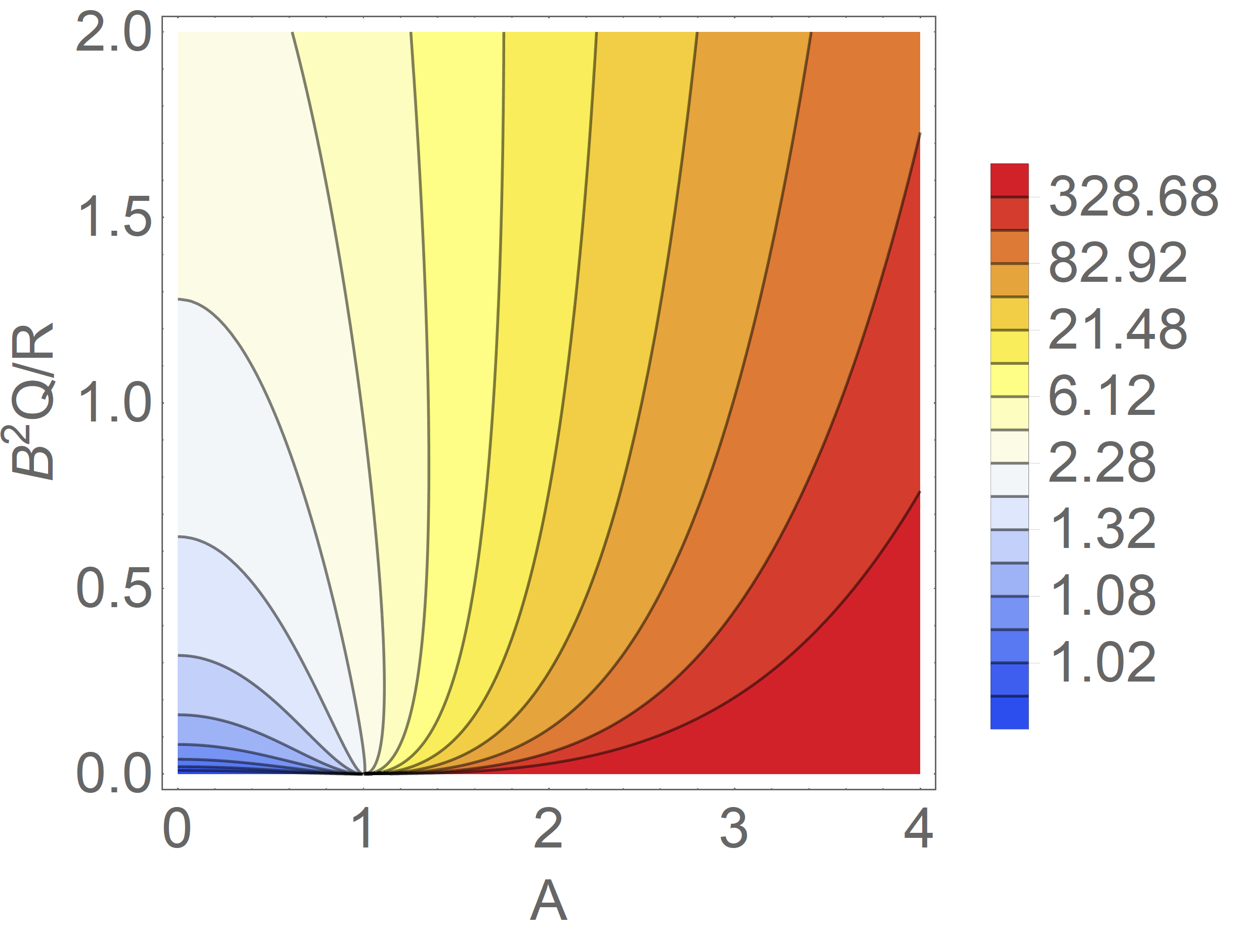
(a) $k=0$.

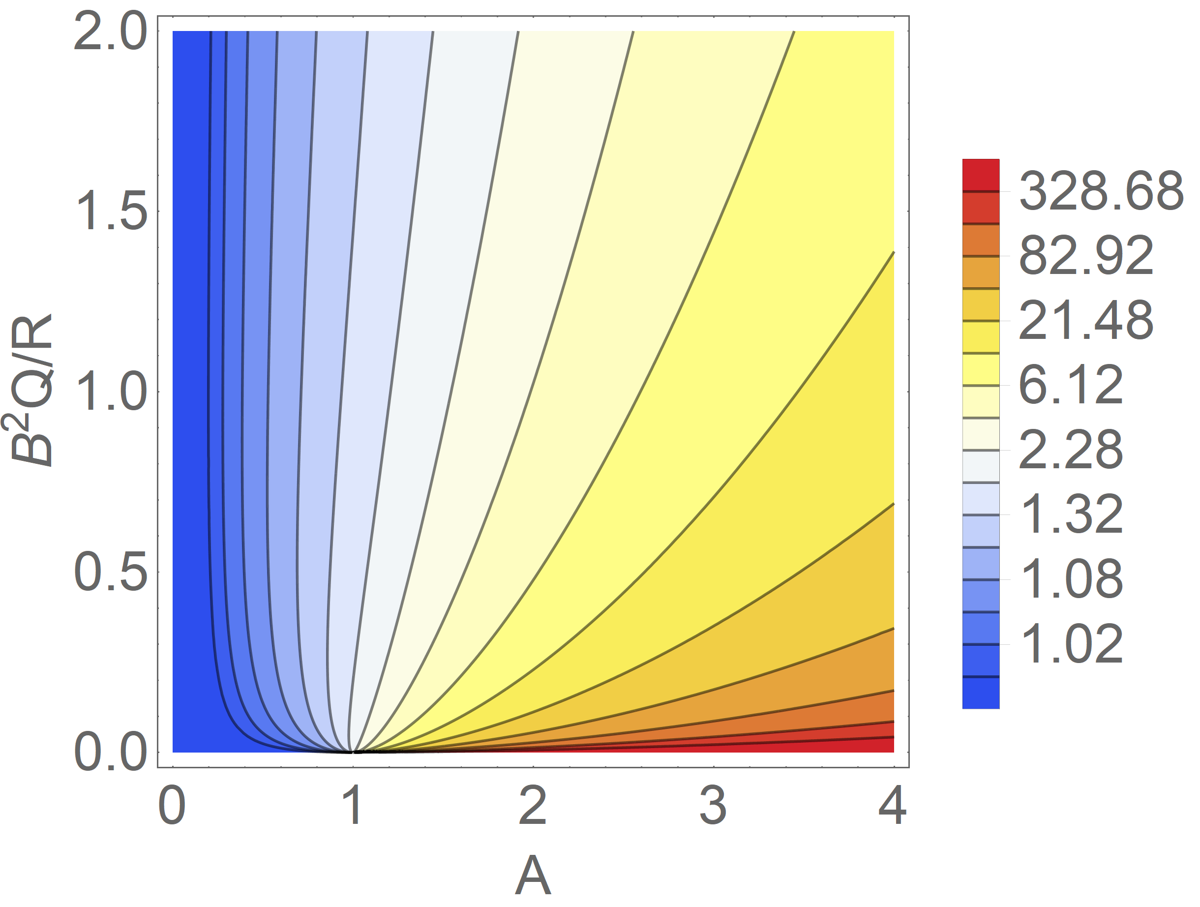
(b) $k=1$.

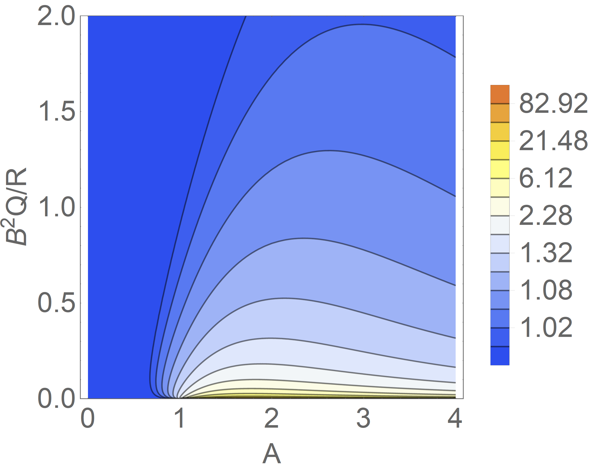
(c) $k=3$.

Figure 1: Illustration of the competitive ratio bound in Corollary 8.1. The system is one-dimensional ($n=m=1$) without delays ($d=0$). With no predictions ($k=0$), the bound is small only if both $A$ and $B^{2}Q/R$ are small. When $k=1$, it is small if $A$ is small or $B^{2}Q/R$ is large. When $k=3$, it is small if $A$ is either small or large, or if $B^{2}Q/R$ is large. The bound is tight in the sense that in some systems, it equals the relative cost of the optimal online policy.

Thus, the competitive ratio exponentially decreases as $k$ goes up. To illustrate how the primary parameters $A$, $B$, $Q$ and $R$ affect the competitive ratio in this case, it is useful to consider the case when $n=m=1$, as shown in both Corollary 8.1 and Figure 1.

Corollary 8.1

Assume there are $k$ exact predictions and no feedback delay, and let $n=m=1$ and $\mathit{Q_{f}}=P$. Then,

$$\frac{\mathsf{Alg}}{\mathsf{Opt}} \leq 1+\frac{2A^{4-2k}}{B^{2}Q/R}\quad \text{if }A^{2}\gg B^{2}Q/R+1,$$

$$\frac{\mathsf{Alg}}{\mathsf{Opt}} \leq 1+\frac{A^{2k}}{(B^{2}Q/R)^{2k-1}}\quad \text{if }B^{2}Q/R\gg A^{2}+1.$$

Interestingly, in this case, the competitive bound only depends on $A^{2}$ and $B^{2}Q/R$. It does not depend on the sign of $A$, nor on $B$, $Q$ or $R$ as long as $B^{2}Q/R$ is fixed. Further, when $k\geq 3$, we see that the competitive ratio is small if $B,Q$ are small, $R$ is large, or $A$ is either very large or very small. However, when $k=0$ or $1$, a large $A$ can result in a large competitive ratio. When $k=0$, a large value of $B^{2}Q/R$ also results in a large competitive ratio. We see below that this is similar to the case of delay (see Section IV-D).

Proposition 9

Theorem 8 is tight in the sense that there exist systems where the competitive ratio of the optimal online algorithm is $1+\Theta(\|F^{k}\|^{2})$.

IV-C Inexact Predictions Without Delay

We next consider the case where predictions are inexact, but there is no feedback delay. The contrast with the previous section highlights the impact of prediction error.

As discussed in Section II-A, the controller should optimize $k$ to utilize predictions with smaller estimation errors while avoiding the use of those with larger errors. The following directly follows from the $d=0$ case of Theorem 4 and reduces to the exact case when $\epsilon_{i}=0$.

Theorem 10

Suppose there are $k$ inexact predictions and no feedback delay. Then,

$$\mathsf{Alg}\leq\bigg{[}\frac{\norm{H}\mathopen{}\mathclose{{}\left(c\sum_{i=0}^{k-1}\epsilon_{i}\|F^{i}\|+\|F^{k}\|}\right)^{2}}{\lambda_{\min}(P^{-1}-FP^{-1}F^{\mathsf{T}}-H)}+1\bigg{]}\mathsf{Opt}+O(1).$$

This subsection differs from the previous one in that the controller can minimize the bound in Theorem 10 with respect to $k$. We characterize this optimization in the following result in 1-d systems, and also provide simulation evidence in Section V (see Figure 3).

Corollary 10.1

Suppose there are $k$ inexact predictions and no feedback delay. Assume $n=m=1$. Given non-decreasing $\{\epsilon_{i}\}$, to minimize the competitive ratio bound in Theorem 10, the optimal number $k$ of predictions to use is such that:

$$\epsilon_{k-1}<\frac{1-\absolutevalue{F}}{1+\absolutevalue{F}}<\epsilon_{k}.$$

The following 1-d setting highlights the dependence of the competitive ratio on the system parameters.

Corollary 10.2

Assume there are $k$ inexact predictions and no feedback delay, and let $n=m=1$ and $\mathit{Q_{f}}=P$.

If $A^{2}\gg B^{2}Q/R+1$,

$$\frac{\mathsf{Alg}}{\mathsf{Opt}}\leq 1+\frac{2A^{4}}{B^{2}Q/R}\mathopen{}\mathclose{{}\left(\sum_{i=0}^{k-1}\frac{\epsilon_{i}}{\absolutevalue{A}^{i}}+\frac{1}{\absolutevalue{A}^{k}}}\right)^{2}.$$

If $B^{2}Q/R\gg A^{2}+1$,

$$\frac{\mathsf{Alg}}{\mathsf{Opt}}\leq 1+\frac{B^{2}Q}{R}\mathopen{}\mathclose{{}\left(\sum_{i=0}^{k-1}\frac{\epsilon_{i}\absolutevalue{A}^{i}}{(B^{2}Q/R)^{i}}+\frac{\absolutevalue{A}^{k}}{(B^{2}Q/R)^{k}}}\right)^{2}.$$

The dependence of the competitive ratio on $A$, $B$, $Q$, $R$ is similar to the case of exact predictions. In particular, we find that the prediction quality in the near future is (exponentially) more important than further in the future, which is consistent with the robust MPC literature [15].

In the exact prediction case we show that Theorem 8 is tight with respect to $\norm{F^{k}}$. In contrast, in the inexact case the tightness of $\epsilon_{i}$ and $\norm{F^{i}}$ in Theorem 10 remains as an open question.

IV-D Delay Without Predictions

The last special case we consider is the case with delays but no (usable) predictions. This case separates the impact of delay from that of predictions. Here, $\hat{w}_{t-d+i|t}=0$ for all $t$ and $i\geq 0$. When $k\leq d$, via Theorem 4 we have that:

$$\mathsf{Alg}\leq\bigg{[}\frac{\norm{H}\mathopen{}\mathclose{{}\left(c\sum_{i=1}^{d}\|A^{i}\|+1}\right)^{2}}{\lambda_{\min}(P^{-1}-FP^{-1}F^{\mathsf{T}}-H)}+1\bigg{]}\mathsf{Opt}+O(1).$$

Depending on whether the spectral radius $\rho(A)<1$, there are two simplifications one can make: (i) if $\rho(A)<1$, then $\|A^{i}\|\leq\kappa a^{i}$ for $a=(\rho(A)+1)/2<1$ for a constant $\kappa$, and (ii) if $\rho(A)>1$, $\|A^{i}\|\leq\|A\|^{i}$.

Theorem 11

Suppose there are $d$ delays and no predictions are available. If $\rho(A)<1$, then the competitive ratio is bounded by a constant irrelevant to the length of delay:

$$\begin{split}\mathsf{Alg}&\leq\bigg{[}\frac{\norm{H}\Big{(}c\kappa\dfrac{a}{1-a}+1\Big{)}^{2}}{\lambda_{\min}(P^{-1}-FP^{-1}F^{\mathsf{T}}-H)}+1\bigg{]}\mathsf{Opt}+O(1).\end{split}$$

If $\rho(A)>1$, then the competitive ratio bound grows exponentially fast with the of number of delay steps:

$$\mathsf{Alg}\leq\bigg{[}\frac{\norm{H}\bigg{(}c\dfrac{\norm{A}^{d+1}-\norm{A}}{\norm{A}-1}+1\bigg{)}^{2}}{\lambda_{\min}(P^{-1}-FP^{-1}F^{\mathsf{T}}-H)}+1\bigg{]}\mathsf{Opt}+O(1).$$

As in the previous subsections, it is useful to consider the one-dimensional case to get insights about the impact of the system parameters.

Corollary 11.1

Assume there are $d$ delays and no predictions. Let $n=m=1$ and $\mathit{Q_{f}}=P$. Then,

$$\frac{\mathsf{Alg}}{\mathsf{Opt}} \leq 1+\frac{2A^{4+2d}}{B^{2}Q/R}\ \text{if }A^{2}\gg B^{2}Q/R+1,$$

$$\frac{\mathsf{Alg}}{\mathsf{Opt}} \leq 1+\frac{A^{2d+2}B^{2}Q/R}{(\absolutevalue{A}-1)^{2}}\ \text{if }B^{2}Q/R\gg A^{2}+1,\,\absolutevalue{A}>1,$$

$$\frac{\mathsf{Alg}}{\mathsf{Opt}} \leq 1+\frac{B^{2}Q/R}{(1-\absolutevalue{A})^{2}}\ \text{if }\absolutevalue{A}<1.$$

Contrary to the case with $k\geq 3$ inexact predictions, when there are delays, a large value of $B^{2}Q/R$ or $A$ does not lead to a small competitive ratio. Instead, in the case of feedback delay, it results in a large competitive ratio. This is consistent with results from robust control theory: the less stable the open loop is ($|A|$ is larger), the more impact delay has [16].

Proposition 12

Theorem 11 is tight in the sense that there exist systems such that the competitive ratio of the optimal online algorithm is at least $1+\Theta(\|A^{d}\|^{2})$.

V NUMERICAL EXAMPLES

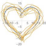
(a) $d=5,\ k=0$.

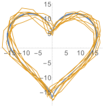
(b) $d=1,\ k=0$.

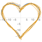
(c) $d=0,\ k=1$.

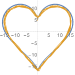
(d) $d=0,\ k=8$.

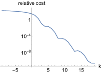
(e) Relative cost: $\mathsf{Alg}/\mathsf{Opt}-1$.

Figure 2: Tracking results with $k$ exact predictions and no delay, or with $d$ steps of delay with no predictions. (a-d) show the desired trajectory (blue) and actual (orange) trajectories. (e) shows both delay and prediction on the x-axis, with the negative part corresponding to delay. The y-axis is in log-scale.

To illustrate our results, we end the paper with numerical examples that highlight the impact of delayed, inexact predictions. To that end, we consider a 2-d tracking problem with the following trajectory [6], illustrated in Figure 2:

$$y_{t}=\begin{bmatrix}16\sin^{3}(\frac{t}{4})\\ 13\cos(\frac{t}{4})-5\cos(\frac{2t}{4})-2\cos(\frac{3t}{4})-\cos(\frac{4t}{4})\end{bmatrix}.$$

We consider following double integrator dynamics:

$$p_{t+1}=p_{t}+0.2v_{t}+h_{t},\quad v_{t+1}=v_{t}+0.2u_{t}+\eta_{t},$$

where $p_{t}\in\mathbb{R}^{2}$ is the position, $v_{t}$ is the velocity, $u_{t}$ is the control, and $h_{t},\eta_{t}\sim\mathrm{U}[-1,1]^{2}$ are i.i.d. noises. The objective is to minimize $\sum_{t=0}^{T-1}\norm{p_{t}-y_{t}}^{2}+0.0016\norm{u_{t}}^{2}$, where we let $T=200$. This problem can be converted to the standard LQR with disturbance $w_{t}$ by letting $x_{t}=\begin{bmatrix}p_{t}\\ v_{t}\end{bmatrix}$ and $\tilde{w}_{t}=\begin{bmatrix}h_{t}\\ \eta_{t}\end{bmatrix}$ and then using the reduction in the LQ tracking example in Section II. Note that the disturbances are the combination of a deterministic trajectory and i.i.d. noise. In contrast, our theoretical results focus on more challenging adversarial disturbances. Nonetheless, the numerical results are consistent with our theorems.

In our first experiment, we study the effect of the number of delays or predictions. For simplicity, we exclude the effect of inexactness of the predictions — a prediction is either exact ($\epsilon_{i}=0$) or uninformative ($\hat{w}_{t-d+i|t}=0$). In this case, each exact prediction cancels a step of delay so, delays can be viewed as “negative” predictions. Figure 2 shows the performance of the proposed myopic policy in Section III with different numbers of predictions or delays. We see that the cost exponentially decreases (increases) as the number of predictions (delays) increases.

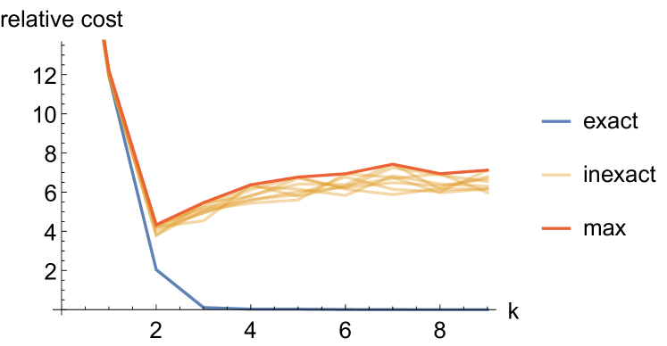
Figure 3: The impact of inexact predictions. The relative cost ($\mathsf{Alg}/\mathsf{Opt}-1$) of MPC using $k$ exact (blue) or inexact (orange) predictions is shown.

In the second experiment, we study the effect of inexact predictions and show that the controller needs to optimize how many predictions are used — it is better to use only a few predictions and ignore those that are too noisy. Specifically, we let $\epsilon_{i}=\frac{1}{5}i^{2}$, i.e., the noise level of predictions grows quadratically fast with the number of steps into the future. Each estimation error $e_{t+i|t}=w_{t+i}-\hat{w}_{t+i|t}$ is independently sampled from $\mathrm{U}[-\epsilon_{i}\norm{w_{t+i}},\epsilon_{i}\norm{w_{t+i}}]^{4}$. This process is repeated 8 times, with each instance depicted by an orange line and their maximum represented by a red line. As shown in Figure 3, with exact predictions, the cost will decrease as the number of predictions increase (the blue line); while with inexact predictions, using fewer predictions may yield better performance.

VI CONCLUDING REMARKS

Our results presens the first constant-competitive policy for general LQR control with adversarial disturbances and delayed imperfect information. We also show that in the case of exact predictions with no delay, or in the case of delay with no predictions, the competitive ratio bounds of the proposed myopic policy match the lower bound. However, in the inexact prediction case, the tightness of $\epsilon_{i}$ in our bounds remains as an open question. Other important extensions include nonlinear dynamics and time-variant linear systems, which can also lead to studying online learning of robust controllers under model mismatch.

-A Cost Characterization Lemma

Before we start our proofs, we first present a technical lemma that is used in many of the proofs below. This lemma connects the control cost of a policy to its difference from the offline optimal policy.

Lemma 13 (Cost characterization)

Suppose at each time $t$, the controller applies the following policy:

$$u_{t}=-(R+B^{\mathsf{T}}PB)^{-1}B^{\mathsf{T}}\mathopen{}\mathclose{{}\left(PAx_{t}+\sum_{i=0}^{T-t-1}{F^{\mathsf{T}}}^{i}Pw_{t+i}-\eta_{t}}\right).$$ (6)

If $\mathit{Q_{f}}=P$, then the control cost is given by:

$$\mathsf{Alg}=\sum_{t=0}^{T-1}\Bigg{(}w_{t}^{\mathsf{T}}Pw_{t}+2w_{t}^{\mathsf{T}}\sum_{i=1}^{T-t-1}{F^{\mathsf{T}}}^{i}Pw_{t+i}-\mathopen{}\mathclose{{}\left(\sum_{i=0}^{T-t-1}{F^{\mathsf{T}}}^{i}Pw_{t+i}}\right)^{\mathsf{T}}H\mathopen{}\mathclose{{}\left(\sum_{i=0}^{T-t-1}{F^{\mathsf{T}}}^{i}Pw_{t+i}}\right)\Bigg{)}+\sum_{t=0}^{T-1}\eta_{t}^{\mathsf{T}}H\eta_{t}\\ +x_{0}^{\mathsf{T}}Px_{0}+2x_{0}^{\mathsf{T}}\sum_{i=0}^{T-1}{F^{\mathsf{T}}}^{i+1}Pw_{i}.$$ (7)

Note that the optimal offline policy has $\eta_{t}=0$ for all $t$ in (7) (as derived by [24]), and as a result, the extra cost of $\mathsf{Alg}$ is given by

$$\mathsf{Alg}-\mathsf{Opt}=\sum_{t=0}^{T-1}\eta_{t}^{\mathsf{T}}H\eta_{t}.$$ (8)

In (6), $\eta_{t}$ can be regarded as the difference between the applied policy and the offline optimal policy.

We also present below a lemma that has appeared in the body, as we will prove the two lemmas at one time.

Lemma 6. For any algorithm, $\mathsf{Alg}(\mathit{Q_{f}})-\mathsf{Opt}^{P}(\mathit{Q_{f}})\leq\mathsf{Alg}(P)-\mathsf{Opt}^{P}(P)+O(1)$, where the $O(1)$ term is with respect to $T$ and it is zero when $\mathit{Q_{f}}=P$.

Proof of Lemmas 13 and 6: Given a disturbance sequence ${\bm{w}}$, we define the cost-to-go function of a policy described by (6):

$$V_{t}^{\mathsf{Alg}}(x_{t};{\bm{w}})\coloneqq\sum_{i=t}^{T-1}(x_{i}^{\mathsf{T}}Qx_{i}+u_{i}^{\mathsf{T}}Ru_{i})+x_{T}^{\mathsf{T}}P_{T}x_{T}=x_{t}^{\mathsf{T}}Qx_{t}+u_{t}^{\mathsf{T}}Ru_{t}+V_{t+1}^{\mathsf{Alg}}(x_{t+1};{\bm{w}}).$$

We will show by backward induction that $V_{t}^{\mathsf{Alg}}(x_{t};{\bm{w}})=x_{t}^{\mathsf{T}}P_{t}x_{t}+x_{t}^{\mathsf{T}}v_{t}+q_{t}$ for some $P_{t}$, $v_{t}$ and $q_{t}$. Let $\Delta_{t}=P_{t}-P$, where $P$ is the solution of DARE (3). When $t=T$, we have $P_{T}=\mathit{Q_{f}}$, $v_{T}=0$ and $q_{T}=0$. Assume this is true at $t+1$. Then,

$$V_{t}^{\mathsf{Alg}}(x_{t};{\bm{w}})$$

$$=x_{t}^{\mathsf{T}}Qx_{t}+u_{t}^{\mathsf{T}}Ru_{t}+(Ax_{t}+Bu_{t}+w_{t})^{\mathsf{T}}P_{t+1}(Ax_{t}+Bu_{t}+w_{t})+(Ax_{t}+Bu_{t}+w_{t})^{\mathsf{T}}v_{t+1}+q_{t+1}$$

$$=u_{t}^{\mathsf{T}}(R+B^{\mathsf{T}}P_{t+1}B)u_{t}+2u_{t}^{\mathsf{T}}B^{\mathsf{T}}(P_{t+1}Ax_{t}+P_{t+1}w_{t}+v_{t+1}/2)$$

$$\quad+x_{t}^{\mathsf{T}}Qx_{t}+(Ax_{t}+w_{t})^{\mathsf{T}}P_{t+1}(Ax_{t}+w_{t})+(Ax_{t}+w_{t})^{\mathsf{T}}v_{t+1}+q_{t+1}$$

$$=u_{t}^{\mathsf{T}}(R+B^{\mathsf{T}}PB)u_{t}+u_{t}^{\mathsf{T}}B^{\mathsf{T}}\Delta_{t+1}Bu_{t}$$

$$\quad+2u_{t}^{\mathsf{T}}B^{\mathsf{T}}(PAx_{t}+Pw_{t}+v_{t+1}/2)+2u_{t}^{\mathsf{T}}B^{\mathsf{T}}(\Delta_{t+1}Ax_{t}+\Delta_{t+1}w_{t}+v_{t+1}/2)$$

$$\quad+x_{t}^{\mathsf{T}}Qx_{t}+(Ax_{t}+w_{t})^{\mathsf{T}}P(Ax_{t}+w_{t})+(Ax_{t}+w_{t})^{\mathsf{T}}\Delta_{t+1}(Ax_{t}+w_{t})+(Ax_{t}+w_{t})^{\mathsf{T}}v_{t+1}+q_{t+1}$$

$$=\mathopen{}\mathclose{{}\left(PAx_{t}+\sum_{i=0}^{T-t-1}{F^{\mathsf{T}}}^{i}Pw_{t+i}-\eta_{t}}\right)^{\mathsf{T}}H\mathopen{}\mathclose{{}\left(PAx_{t}+\sum_{i=0}^{T-t-1}{F^{\mathsf{T}}}^{i}Pw_{t+i}-\eta_{t}}\right)$$

$$\quad+\mathopen{}\mathclose{{}\left(PAx_{t}+\sum_{i=0}^{T-t-1}{F^{\mathsf{T}}}^{i}Pw_{t+i}-\eta_{t}}\right)^{\mathsf{T}}H\Delta_{t+1}H\mathopen{}\mathclose{{}\left(PAx_{t}+\sum_{i=0}^{T-t-1}{F^{\mathsf{T}}}^{i}Pw_{t+i}-\eta_{t}}\right)$$

$$\quad-2\mathopen{}\mathclose{{}\left(PAx_{t}+\sum_{i=0}^{T-t-1}{F^{\mathsf{T}}}^{i}Pw_{t+i}-\eta_{t}}\right)^{\mathsf{T}}H(PAx_{t}+Pw_{t}+v_{t+1}/2)$$

$$\quad-2\mathopen{}\mathclose{{}\left(PAx_{t}+\sum_{i=0}^{T-t-1}{F^{\mathsf{T}}}^{i}Pw_{t+i}-\eta_{t}}\right)^{\mathsf{T}}H(\Delta_{t+1}Ax_{t}+\Delta_{t+1}w_{t}+v_{t+1}/2)$$

$$\quad+x_{t}^{\mathsf{T}}Qx_{t}+(Ax_{t}+w_{t})^{\mathsf{T}}P(Ax_{t}+w_{t})+(Ax_{t}+w_{t})^{\mathsf{T}}\Delta_{t+1}(Ax_{t}+w_{t})+(Ax_{t}+w_{t})^{\mathsf{T}}v_{t+1}+q_{t+1}$$

$$=(PAx_{t})^{\mathsf{T}}H(PAx_{t})+2(PAx_{t})^{\mathsf{T}}H\mathopen{}\mathclose{{}\left(\sum_{i=0}^{T-t-1}{F^{\mathsf{T}}}^{i}Pw_{t+i}-\eta_{t}}\right)$$

$$\quad+\mathopen{}\mathclose{{}\left(\sum_{i=0}^{T-t-1}{F^{\mathsf{T}}}^{i}Pw_{t+i}-\eta_{t}}\right)^{\mathsf{T}}H\mathopen{}\mathclose{{}\left(\sum_{i=0}^{T-t-1}{F^{\mathsf{T}}}^{i}Pw_{t+i}-\eta_{t}}\right)$$

$$\quad+(PAx_{t})^{\mathsf{T}}H\Delta_{t+1}H(PAx_{t})+2(PAx_{t})^{\mathsf{T}}H\Delta_{t+1}H\mathopen{}\mathclose{{}\left(\sum_{i=0}^{T-t-1}{F^{\mathsf{T}}}^{i}Pw_{t+i}-\eta_{t}}\right)$$

$$\quad+\mathopen{}\mathclose{{}\left(\sum_{i=0}^{T-t-1}{F^{\mathsf{T}}}^{i}Pw_{t+i}-\eta_{t}}\right)^{\mathsf{T}}H\Delta_{t+1}H\mathopen{}\mathclose{{}\left(\sum_{i=0}^{T-t-1}{F^{\mathsf{T}}}^{i}Pw_{t+i}-\eta_{t}}\right)$$

$$\quad-2\mathopen{}\mathclose{{}\left(PAx_{t}}\right)^{\mathsf{T}}H(PAx_{t}+Pw_{t}+v_{t+1}/2)-2\mathopen{}\mathclose{{}\left(\sum_{i=0}^{T-t-1}{F^{\mathsf{T}}}^{i}Pw_{t+i}-\eta_{t}}\right)^{\mathsf{T}}H(PAx_{t}+Pw_{t}+v_{t+1}/2)$$

$$\quad-2\mathopen{}\mathclose{{}\left(PAx_{t}}\right)^{\mathsf{T}}H\Delta_{t+1}(Ax_{t}+w_{t})-2\mathopen{}\mathclose{{}\left(\sum_{i=0}^{T-t-1}{F^{\mathsf{T}}}^{i}Pw_{t+i}-\eta_{t}}\right)^{\mathsf{T}}H\Delta_{t+1}(Ax_{t}+w_{t})$$

$$\quad+x_{t}^{\mathsf{T}}Qx_{t}+(Ax_{t}+w_{t})^{\mathsf{T}}P(Ax_{t}+w_{t})+(Ax_{t}+w_{t})^{\mathsf{T}}\Delta_{t+1}(Ax_{t}+w_{t})+(Ax_{t}+w_{t})^{\mathsf{T}}v_{t+1}+q_{t+1}$$

$$=x_{t}^{\mathsf{T}}(Q+A^{\mathsf{T}}PA-A^{\mathsf{T}}PHPA+F^{\mathsf{T}}\Delta_{t+1}F)x_{t}$$

$$\quad+2x_{t}^{\mathsf{T}}F^{\mathsf{T}}P_{t+1}w_{t}+x_{t}^{\mathsf{T}}F^{\mathsf{T}}v_{t+1}-x_{t}^{\mathsf{T}}F^{\mathsf{T}}\Delta_{t+1}H\mathopen{}\mathclose{{}\left(\sum_{i=0}^{T-t-1}{F^{\mathsf{T}}}^{i}Pw_{t+i}-\eta_{t}}\right)$$

$$\quad+\mathopen{}\mathclose{{}\left(\sum_{i=0}^{T-t-1}{F^{\mathsf{T}}}^{i}Pw_{t+i}-\eta_{t}}\right)^{\mathsf{T}}H\mathopen{}\mathclose{{}\left(\sum_{i=0}^{T-t-1}{F^{\mathsf{T}}}^{i}Pw_{t+i}-\eta_{t}}\right)-2\mathopen{}\mathclose{{}\left(\sum_{i=0}^{T-t-1}{F^{\mathsf{T}}}^{i}Pw_{t+i}-\eta_{t}}\right)^{\mathsf{T}}H(Pw_{t}+v_{t+1}/2)$$

$$\quad+w_{t}^{\mathsf{T}}Pw_{t}+w_{t}^{\mathsf{T}}v_{t+1}+q_{t+1}+O(\Delta_{t+1}).$$

Thus, $P+\Delta_{t}=P_{t}=Q+A^{\mathsf{T}}PA-A^{\mathsf{T}}PHPA+F^{\mathsf{T}}\Delta_{t+1}F=P+F^{\mathsf{T}}\Delta_{t+1}F$ and thus $\Delta_{t}=F^{\mathsf{T}}\Delta_{t+1}F=O(\lambda^{2(T-t)})$, where $\lambda=\frac{1+\rho(F)}{2}$. The recursive formulae for $v_{t}$ and $q_{t}$ are given by:

$$v_{t} =2F^{\mathsf{T}}Pw_{t}+F^{\mathsf{T}}v_{t+1}+O(\lambda^{2(T-t)})=2\sum_{i=0}^{T-t-1}{F^{\mathsf{T}}}^{i+1}Pw_{t+i}+O(\lambda^{T-t})$$

$$v_{t+1} =2\sum_{i=1}^{T-t-1}{F^{\mathsf{T}}}^{i}Pw_{t+i}+O(\lambda^{T-t}),$$

$$q_{t} =q_{t+1}+w_{t}^{\mathsf{T}}Pw_{t}+2w_{t}^{\mathsf{T}}\sum_{i=1}^{T-t-1}{F^{\mathsf{T}}}^{i}Pw_{t+i}+\mathopen{}\mathclose{{}\left(\sum_{i=0}^{T-t-1}{F^{\mathsf{T}}}^{i}Pw_{t+i}-\eta_{t}}\right)^{\mathsf{T}}H\mathopen{}\mathclose{{}\left(\sum_{i=0}^{T-t-1}{F^{\mathsf{T}}}^{i}Pw_{t+i}-\eta_{t}}\right)$$

$$\quad-2\mathopen{}\mathclose{{}\left(\sum_{i=0}^{T-t-1}{F^{\mathsf{T}}}^{i}Pw_{t+i}-\eta_{t}}\right)^{\mathsf{T}}H\mathopen{}\mathclose{{}\left(\sum_{i=0}^{T-t-1}{F^{\mathsf{T}}}^{i}Pw_{t+i}+O(\lambda^{T-t})}\right)+O(\lambda^{T-t})$$

$$=q_{t+1}+w_{t}^{\mathsf{T}}Pw_{t}+2w_{t}^{\mathsf{T}}\sum_{i=1}^{T-t-1}{F^{\mathsf{T}}}^{i}Pw_{t+i}-\mathopen{}\mathclose{{}\left(\sum_{i=0}^{T-t-1}{F^{\mathsf{T}}}^{i}Pw_{t+i}}\right)^{\mathsf{T}}H\mathopen{}\mathclose{{}\left(\sum_{i=0}^{T-t-1}{F^{\mathsf{T}}}^{i}Pw_{t+i}}\right)+\eta_{t}^{\mathsf{T}}H\eta_{t}$$

$$\quad+O(\lambda^{T-t}).$$

Then,

$$\begin{split}\mathsf{Alg}&=V_{0}^{\mathsf{Alg}}(x_{0};{\bm{w}})=x_{0}^{\mathsf{T}}P_{0}x_{0}+x_{0}^{\mathsf{T}}v_{0}+q_{0}\\ &=x_{0}^{\mathsf{T}}P_{0}x_{0}+x_{0}^{\mathsf{T}}\mathopen{}\mathclose{{}\left(2\sum_{i=0}^{T-1}{F^{\mathsf{T}}}^{i+1}Pw_{i}+O(\lambda^{T})}\right)+\sum_{t=0}^{T-1}\eta_{t}^{\mathsf{T}}H\eta_{t}+\sum_{t=0}^{T-1}O(\lambda^{T-t})\\ &\quad+\sum_{t=0}^{T-1}\Bigg{(}w_{t}^{\mathsf{T}}Pw_{t}+2w_{t}^{\mathsf{T}}\sum_{i=1}^{T-t-1}{F^{\mathsf{T}}}^{i}Pw_{t+i}-\mathopen{}\mathclose{{}\left(\sum_{i=0}^{T-t-1}{F^{\mathsf{T}}}^{i}Pw_{t+i}}\right)^{\mathsf{T}}H\mathopen{}\mathclose{{}\left(\sum_{i=0}^{T-t-1}{F^{\mathsf{T}}}^{i}Pw_{t+i}}\right)\Bigg{)}.\end{split}$$

If $\mathit{Q_{f}}=P$, then the above $O(\lambda^{T})$ and $O(\lambda^{T-t})$ are both zero and thus we obtain (7). Otherwise,

$$\mathsf{Alg}(\mathit{Q_{f}})-\mathsf{Opt}^{P}(\mathit{Q_{f}})=x_{0}^{\mathsf{T}}O(\lambda^{T})+\sum_{t=0}^{T-1}\eta_{t}^{\mathsf{T}}H\eta_{t}+O(1).$$

Therefore, $(\mathsf{Alg}(\mathit{Q_{f}})-\mathsf{Opt}^{P}(\mathit{Q_{f}}))-(\mathsf{Alg}(P)-\mathsf{Opt}^{P}(P))=O(1)$.

-B Proof of Theorem 3

Theorem 3. Suppose there are $d$ delays and $k$ exact predictions with $k<d$. Assume all used predictions are exact and other disturbances (with unused predictions) are zero. The optimal policy at time $t$ is:

$$u_{t}=-(R+B^{\mathsf{T}}PB)^{-1}B^{\mathsf{T}}PA\mathopen{}\mathclose{{}\left(A^{d-k}\hat{x}_{t-d+k|t}+\sum_{i=0}^{d-k-1}A^{i}Bu_{t-1-i}}\right).$$ (5)

Proof:

Lemma 13 implies that when $\mathit{Q_{f}}=P$, the offline optimal policy is given by

$$u_{t}=-(R+B^{\mathsf{T}}PB)^{-1}B^{\mathsf{T}}\mathopen{}\mathclose{{}\left(PAx_{t}+\sum_{i=0}^{T-t-1}{F^{\mathsf{T}}}^{i}Pw_{t+i}}\right).$$

However, we are looking for the optimal policy using the incorrect assumptions that (i) $w_{t-d+k}$ and all later disturbances are zero, and (ii) $w_{t-d},\dots,w_{t-d+k-1}$ equals to $\hat{w}_{t-d|t},\dots,\hat{w}_{t-d+k-1|t}$ respectively.

Replacing $w_{t+i}$ by zero and $x_{t}$ by $\hat{x}_{t|t}$ in the above policy, we obtain:

$$u_{t}=-(R+B^{\mathsf{T}}PB)^{-1}B^{\mathsf{T}}PA\hat{x}_{t|t}.$$ (9)

$$\begin{split}\hat{x}_{t|t}&=A\hat{x}_{t-1|t}+Bu_{t-1}\\ &=A(A\hat{x}_{t-2|t}+Bu_{t-2})+Bu_{t-1}\\ &\quad\vdots\\ &=A^{d-k}\hat{x}_{t-d+k|t}+A^{d-k-1}Bu_{t-d+k}+\dots+Bu_{t-1}\\ &=A^{d-k}\hat{x}_{t-d+k|t}+\sum_{i=0}^{d-k-1}A^{i}Bu_{t-1-i}.\end{split}$$

As such, we obtain Theorem 3. ∎

-C Proof of Theorem 4

Theorem 4. Let $c=\norm{P}\|P^{-1}\|(1+\norm{F})$ and $H=B(R+B^{\mathsf{T}}PB)^{-1}B^{\mathsf{T}}$. Suppose there are $d$ steps of delays and the controller uses $k$ predictions. When $k\geq d$,

$$\mathsf{Alg}\leq\Bigg{[}\frac{\mathopen{}\mathclose{{}\left(c\sum\limits_{i=0}^{d-1}\epsilon_{i}\|A^{d-i}\|+c\sum\limits_{i=d}^{k-1}\epsilon_{i}\|F^{i-d}\|+\|F^{k-d}\|}\right)^{2}}{\norm{H}^{-1}\lambda_{\min}(P^{-1}-FP^{-1}F^{\mathsf{T}}-H)}+1\Bigg{]}\mathsf{Opt}+O(1).$$

When $k\leq d$,

$$\mathsf{Alg}\leq\Bigg{[}\frac{\bigg{(}c\sum\limits_{i=0}^{k-1}\epsilon_{i}\|A^{d-i}\|+c\sum\limits_{i=k}^{d-1}\|A^{d-i}\|+1\bigg{)}^{2}}{\norm{H}^{-1}\lambda_{\min}(P^{-1}-FP^{-1}F^{\mathsf{T}}-H)}+1\Bigg{]}\mathsf{Opt}+O(1).$$

The $O(1)$ is with respect to $T$. It may depend on the system parameters $A$, $B$, $Q$, $R$, $\mathit{Q_{f}}$ and the range of disturbances $r$, but not on $T$. When $\mathit{Q_{f}}=P$ the $O(1)$ is zero.

The proof outline provided in the body lays out a set of lemmas that, together, prove Theorem 4. Here, we provide proofs for each of them.

-D Proof of Lemma 5

Lemma 5. Suppose $\mathit{Q_{f}}=P$. Then, the conclusion of Theorem 4 holds.

Proof:

This lemma considers the case of $\mathit{Q_{f}}=P$. Lemma 13 implies that when $\mathit{Q_{f}}=P$, the cost of the offline optimal policy is:

$$\mathsf{Opt}=\sum_{t=0}^{T-1}\Bigg{(}w_{t}^{\mathsf{T}}Pw_{t}+2w_{t}^{\mathsf{T}}\sum_{i=1}^{T-t-1}{F^{\mathsf{T}}}^{i}Pw_{t+i}-\mathopen{}\mathclose{{}\left(\sum_{i=0}^{T-t-1}{F^{\mathsf{T}}}^{i}Pw_{t+i}}\right)^{\mathsf{T}}H\mathopen{}\mathclose{{}\left(\sum_{i=0}^{T-t-1}{F^{\mathsf{T}}}^{i}Pw_{t+i}}\right)\Bigg{)}\\ +x_{0}^{\mathsf{T}}Px_{0}+2x_{0}^{\mathsf{T}}\sum_{i=0}^{T-1}{F^{\mathsf{T}}}^{i+1}Pw_{i}.$$

We consider the following substitution:

$$\psi_{t}=\sum_{i=0}^{T-t-1}{F^{\mathsf{T}}}^{i}Pw_{t+i},\quad w_{t}=P^{-1}(\psi_{t}-F^{\mathsf{T}}\psi_{t+1}).$$ (10)

Then, the offline optimal cost can be lower bounded:

$$\begin{split}\mathsf{Opt}&=\sum_{t=0}^{T-1}(w_{t}^{\mathsf{T}}Pw_{t}+2w_{t}^{\mathsf{T}}F^{\mathsf{T}}\psi_{t+1}-\psi_{t}^{\mathsf{T}}H\psi_{t})+x_{0}^{\mathsf{T}}Px_{0}+2x_{0}^{\mathsf{T}}F^{\mathsf{T}}\psi_{0}\\ &=\sum_{t=0}^{T-1}(\psi_{t}^{\mathsf{T}}P^{-1}\psi_{t}-\psi_{t+1}^{\mathsf{T}}FP^{-1}F^{\mathsf{T}}\psi_{t+1}-\psi_{t}^{\mathsf{T}}H\psi_{t})+x_{0}^{\mathsf{T}}Px_{0}+2x_{0}^{\mathsf{T}}F^{\mathsf{T}}\psi_{0}\\ &=\sum_{t=0}^{T-1}(\psi_{t}^{\mathsf{T}}P^{-1}\psi_{t}-\psi_{t}^{\mathsf{T}}FP^{-1}F^{\mathsf{T}}\psi_{t}-\psi_{t}^{\mathsf{T}}H\psi_{t})+\psi_{0}^{\mathsf{T}}FP^{-1}F^{\mathsf{T}}\psi_{0}+x_{0}^{\mathsf{T}}Px_{0}+2x_{0}^{\mathsf{T}}F^{\mathsf{T}}\psi_{0}\\ &=\sum_{t=0}^{T-1}\psi_{t}^{\mathsf{T}}(P^{-1}-FP^{-1}F^{\mathsf{T}}-H)\psi_{t}+(F^{\mathsf{T}}\psi_{0}+Px_{0})^{\mathsf{T}}P^{-1}(F^{\mathsf{T}}\psi_{0}+Px_{0})\\ &\geq\lambda_{\min}(P^{-1}-FP^{-1}F^{\mathsf{T}}-H)\sum_{t=0}^{T-1}\norm{\psi_{t}}^{2}.\end{split}$$ (11)

The myopic policy has two cases and we analyze each of them below.

Case 1: $k\geq d$

In this case, the controller estimates $x_{t}$ using $x_{t-d}$ and $\hat{w}_{t-d|t},\dots,\hat{w}_{t-1|t}$.

$$x_{t}-\hat{x}_{t|t}=(Ax_{t-1}+Bu_{t-1}+w_{t-1})-(A\hat{x}_{t-1|t}+Bu_{t-1}+\hat{w}_{t-1|t})=A(x_{t-1}-\hat{x}_{t-1|t})+e_{t-1|t}.$$

Applying similar procedures repetitively, we obtain:

$$x_{t}-\hat{x}_{t|t}=e_{t-1|t}+Ae_{t-2|t}+\dots+A^{d-1}e_{t-d|t}=\sum_{i=1}^{d}A^{i-1}e_{t-i|t}.$$

Comparing Equations 4 and 6, we have

$$\eta_{t}=\sum_{i=1}^{d}PA^{i}e_{t-i|t}+\sum_{i=0}^{k-d-1}{F^{\mathsf{T}}}^{i}Pe_{t+i|t}+\sum_{i=k-d}^{T-t-1}{F^{\mathsf{T}}}^{i}Pw_{t+i}.$$ (12)

Using the substitution in (10), we bound (12) as follows.

$$\begin{split}\norm{\eta_{t}}&=\norm{\sum_{i=1}^{d}PA^{i}e_{t-i|t}+\sum_{i=0}^{k-d-1}{F^{\mathsf{T}}}^{i}Pe_{t+i|t}+{F^{\mathsf{T}}}^{k-d}\psi_{t+k-d}}\\ &\leq\sum_{i=1}^{d}\norm{P}\norm{A^{i}}\epsilon_{d-i}\norm{w_{t-i}}+\sum_{i=0}^{k-d-1}\norm{F^{i}}\norm{P}\epsilon_{i-d}\norm{w_{t+i}}+\norm{F^{k-d}}\norm{\psi_{t+k-d}}\\ &\leq\sum_{i=1}^{d}\norm{P}\norm{A^{i}}\epsilon_{d-i}\norm{P^{-1}}(\norm{\psi_{t-i}}+\norm{F}\norm{\psi_{t-i+1}})\\ &\quad+\sum_{i=0}^{k-d-1}\norm{F^{i}}\norm{P}\epsilon_{i-d}\norm{P^{-1}}(\norm{\psi_{t+i}}+\norm{F}\norm{\psi_{t+i+1}})+\norm{F^{k-d}}\norm{\psi_{t+k-d}}.\end{split}$$ (13)

Note that when $t<d$, some terms in (13) have negative subscripts. Those terms do not actually exist and should be regarded as zero. However, for the clarity of the proof, we keep them in the formula. In the later derivations, although we treat them as potentially non-zero, they do not affect our result because we are looking for an upper bound. Let $\bm{\eta}=(\|\eta_{0}\|,\dots,\|\eta_{T-1}\|)\in\mathbb{R}^{T}$ and $\bm{\psi}=(\|\psi_{0}\|,\dots,\|\psi_{T-1}\|)$. Equation 13 provides a linear inequality relationship between $\bm{\eta}$ and $\bm{\psi}$. We define matrix $M=\{M_{t,s}\}_{t,s=0}^{T-1}\in\mathbb{R}^{T\times T}$ such that $M_{t,s}$ is the coefficient of $\|\psi_{s}\|$ in the bound of $\|\eta_{t}\|$ in (13). Then, $\bm{\eta}\leq M\bm{\psi}$.

$$\sum_{t=0}^{T-1}\eta_{t}^{\mathsf{T}}H\eta_{t}\leq\norm{H}\bm{\eta}^{\mathsf{T}}\bm{\eta}\leq\norm{H}\bm{\psi}^{\mathsf{T}}M^{\mathsf{T}}M\bm{\psi}\leq\lambda_{\max}(M^{\mathsf{T}}M)\norm{H}\norm{\bm{\psi}}^{2}.$$ (14)

Proposition 14 (Gershgorin circle theorem)

Let $A\in\mathbb{C}^{n\times n}$. Let $D(A_{i,i},R_{i})\subseteq\mathbb{C}$ be a closed disc centered at $A_{i,i}$ with radius $R_{i}=\sum_{j\neq i}\absolutevalue{A_{i,j}}$. Then, every eigenvalue of $A$ lies within at least one of the discs $D(A_{i,i},R_{i})$.

We use Proposition 14 to bound the eigenvalues of $M^{\mathsf{T}}M$:

$$\lambda_{\max}(M^{\mathsf{T}}M)\leq\max_{i}\sum_{j=0}^{T-1}(M^{\mathsf{T}}M)_{i,j}=\norm{M^{\mathsf{T}}M\bm{1}}_{\infty}.$$ (15)

Plugging $\norm{\psi_{s}}=1$ for all $s$ into (13), we have:

$$M\bm{1}\leq\mathopen{}\mathclose{{}\left(\norm{P}\norm{P^{-1}}(1+\norm{F})\mathopen{}\mathclose{{}\left(\sum_{i=1}^{d}\norm{A^{i}}\epsilon_{d-i}+\sum_{i=0}^{k-d-1}\norm{F^{i}}\epsilon_{i-d}}\right)+\norm{F^{k-d}}}\right)\bm{1}.$$

Thus, (15) can be further bounded:

$$\lambda_{\max}(M^{\mathsf{T}}M)\leq\mathopen{}\mathclose{{}\left(c\mathopen{}\mathclose{{}\left(\sum_{i=1}^{d}\norm{A^{i}}\epsilon_{d-i}+\sum_{i=0}^{k-d-1}\norm{F^{i}}\epsilon_{i-d}}\right)+\norm{F^{k-d}}}\right)^{2},$$

where $c=\norm{P}\norm{P^{-1}}(1+\norm{F})$. Together with Equations 8 and 14, this implies that

$$\mathsf{Alg}-\mathsf{Opt}=\sum_{t=0}^{T-1}\eta_{t}^{\mathsf{T}}H\eta_{t}\leq\mathopen{}\mathclose{{}\left(c\mathopen{}\mathclose{{}\left(\sum_{i=1}^{d}\norm{A^{i}}\epsilon_{d-i}+\sum_{i=0}^{k-d-1}\norm{F^{i}}\epsilon_{i-d}}\right)+\norm{F^{k-d}}}\right)^{2}\norm{H}\norm{\bm{\psi}}^{2}.$$

Together with (11), we have

$$\frac{\mathsf{Alg}-\mathsf{Opt}}{\mathsf{Opt}}\leq\mathopen{}\mathclose{{}\left(c\mathopen{}\mathclose{{}\left(\sum_{i=1}^{d}\norm{A^{i}}\epsilon_{d-i}+\sum_{i=0}^{k-d-1}\norm{F^{i}}\epsilon_{i-d}}\right)+\norm{F^{k-d}}}\right)^{2}\norm{H}\lambda_{\min}^{-1}(P^{-1}-FP^{-1}F^{\mathsf{T}}-H).$$

Case 2: $k<d$

We start from (9). In this case, we have the following equations.

$$x_{t}-\hat{x}_{t|t} =A(x_{t-1}-\hat{x}_{t-1|t})+w_{t-1}-0.$$

$$\vdots$$

$$x_{t-d+k+1}-\hat{x}_{t-d+k+1|t} =A(x_{t-d+k}-\hat{x}_{t-d+k|t})+w_{t-d+k}-0.$$

$$x_{t-d+k}-\hat{x}_{t-d+k|t} =A(x_{t-d+k-1}-\hat{x}_{t-d+k-1|t})+w_{t-d+k-1}-\hat{w}_{t-d+k-1|t}.$$

$$\vdots$$

$$x_{t-d+1}-\hat{x}_{t-d+1|t} =A(x_{t-d}-\hat{x}_{t-d|t})+w_{t-d}-\hat{w}_{t-d|t}.$$

Note that in the last line, $x_{t-d}=\hat{x}_{t-d|t}$. Thus, all of the above equations can be combined into the following:

$$x_{t}-\hat{x}_{t|t}=\sum_{i=0}^{k-1}A^{d-i-1}e_{t-d+i|t}+\sum_{i=k}^{d-1}A^{d-i-1}w_{t-d+i}.$$

Therefore, the policy can be written as:

$$\begin{split}u_{t}&=-(R+B^{\mathsf{T}}PB)^{-1}B^{\mathsf{T}}PA\hat{x}_{t|t}\\ &=-(R+B^{\mathsf{T}}PB)^{-1}B^{\mathsf{T}}PA\mathopen{}\mathclose{{}\left(x_{t}-\sum_{i=0}^{k-1}A^{d-i-1}e_{t-d+i|t}-\sum_{i=k}^{d-1}A^{d-i-1}w_{t-d+i}}\right).\end{split}$$

We compare this with (6) to get

$$\eta_{t}=\sum_{i=0}^{k-1}PA^{d-i}e_{t-d+i|t}+\sum_{i=k}^{d-1}PA^{d-i}w_{t-d+i}+\sum_{i=0}^{T-t-1}{F^{\mathsf{T}}}^{i}Pw_{t+i}.$$

With the substitution in (10),

$$\begin{split}\norm{\eta_{t}}&=\norm{\sum_{i=0}^{k-1}PA^{d-i}e_{t-d+i|t}+\sum_{i=k}^{d-1}PA^{d-i}w_{t-d+i}+\psi_{t}}\\ &\leq\sum_{i=0}^{k-1}\norm{P}\norm{A^{d-i}}\epsilon_{i}\norm{w_{t-d+i}}+\sum_{i=k}^{d-1}\norm{P}\norm{A^{d-i}}\norm{w_{t-d+i}}+\norm{\psi_{t}}\\ &\leq\sum_{i=0}^{k-1}\norm{P}\norm{A^{d-i}}\epsilon_{i}\norm{P^{-1}}(\norm{\psi_{t-d+i}}+\norm{F}\norm{\psi_{t-d+i+1}})\\ &\quad+\sum_{i=k}^{d-1}\norm{P}\norm{A^{d-i}}\norm{P^{-1}}(\norm{\psi_{t-d+i}}+\norm{F}\norm{\psi_{t-d+i+1}})+\norm{\psi_{t}}.\end{split}$$ (16)

Similar to the previous case, we define matrix $M=\{M_{t,s}\}_{t,s=0}^{T-1}\in\mathbb{R}^{T\times T}$ such that $M_{t,s}$ is the coefficient of $\|\psi_{s}\|$ in the bound of $\|\eta_{t}\|$ in (16). Then, by Proposition 14,

$$\lambda_{\max}(M^{\mathsf{T}}M)\leq\mathopen{}\mathclose{{}\left(c\sum_{i=0}^{k-1}\norm{A^{d-i}}\epsilon_{i}+c\sum_{i=k}^{d-1}\norm{A^{d-i}}+\norm{\psi_{t}}}\right)^{2}.$$

$$\mathsf{Alg}-\mathsf{Opt}=\sum_{t=0}^{T-1}\eta_{t}^{\mathsf{T}}H\eta_{t}\leq\norm{H}\bm{\eta}^{\mathsf{T}}\bm{\eta}\leq\norm{H}\bm{\psi}^{\mathsf{T}}M^{\mathsf{T}}M\bm{\psi}\leq\lambda_{\max}(M^{\mathsf{T}}M)\norm{H}\norm{\bm{\psi}}^{2}.$$

$$\frac{\mathsf{Alg}-\mathsf{Opt}}{\mathsf{Opt}}\leq\mathopen{}\mathclose{{}\left(c\sum_{i=0}^{k-1}\norm{A^{d-i}}\epsilon_{i}+c\sum_{i=k}^{d-1}\norm{A^{d-i}}+\norm{\psi_{t}}}\right)^{2}\norm{H}\lambda_{\min}^{-1}(P^{-1}-FP^{-1}F^{\mathsf{T}}-H).$$

∎

-E Proof of Lemma 6

See Section -A.

-F Proof of Lemma 7

Lemma 7. The followings are equal up to $O(1)$ difference: $\mathsf{Opt}^{P}(P),\ \mathsf{Opt}^{P}(\mathit{Q_{f}}),\ \mathsf{Opt}^{\mathit{Q_{f}}}(\mathit{Q_{f}})$.

Proof:

By definition,

$$\mathsf{Opt}^{P}(P)=\min_{X}\mathsf{Opt}^{X}(P)\leq\mathsf{Opt}^{\mathit{Q_{f}}}(P),$$

$$\mathsf{Opt}^{\mathit{Q_{f}}}(\mathit{Q_{f}})=\min_{X}\mathsf{Opt}^{X}(\mathit{Q_{f}})\leq\mathsf{Opt}^{P}(\mathit{Q_{f}}).$$

Moreover, for any $X$,

$$\mathsf{Opt}^{X}(\mathit{Q_{f}})-\mathsf{Opt}^{X}(P)=x_{T}^{\mathsf{T}}(\mathit{Q_{f}}-P)x_{T}=O(1),$$

where $x_{T}$ is the final state obtained by the policy that is optimal assuming the terminal cost is $X$. Therefore,

$$\mathsf{Opt}^{P}(P)\leq\mathsf{Opt}^{\mathit{Q_{f}}}(P)=\mathsf{Opt}^{\mathit{Q_{f}}}(\mathit{Q_{f}})+O(1)\leq\mathsf{Opt}^{P}(\mathit{Q_{f}})+O(1)=\mathsf{Opt}^{P}(P)+O(1).$$

As a result, $\mathsf{Opt}^{P}(P),\mathsf{Opt}^{P}(\mathit{Q_{f}}),\mathsf{Opt}^{\mathit{Q_{f}}}(\mathit{Q_{f}}),\mathsf{Opt}^{\mathit{Q_{f}}}(P)$ are all equal up to a difference of $O(1)$.∎

-G Tightness of Theorem 8

The lower bound is obtained in the setting where all disturbances $\{w_{t}\}$ are i.i.d. with zero mean.

Suppose there are $k$ exact predictions and no delays. Let $n=m=1$. It has been shown [7, Theorem 3.2] that the average cost per time step of the optimal online policy is given by

$$PW-\sum_{i=0}^{k-1}F^{2i}P^{2}HW,$$

where $W$ is the variance of the disturbances. The minimum offline cost is obtained by taking $k\to\infty$. Thus,

$$\mathsf{Alg}-\mathsf{Opt}=\sum_{i=k}^{\infty}F^{2i}P^{2}HW=\Theta(F^{2k}).$$

As a result,

$$\frac{\mathsf{Alg}}{\mathsf{Opt}}=1+\Theta(F^{2k}).$$

This one-dimensional example generalizes to higher dimensions by stacking independent one-dimensional systems together, so that all matrices are diagonal.

-H Tightness of Theorem 11

For the case of $d$ steps of delay and no usable predictions, we can derive a lower bound for the cost of the optimal online policy in the setting of i.i.d. noise with zero mean.

Let $n=m=1$ and assume $\rho(A)>1$. Using a similar dynamic programming approach, we can get the cost per time step of the optimal online policy facing $d$ steps of delays, given by

$$A^{2d}PW+\sum_{i=0}^{d-1}A^{2i}QW=\Theta(A^{2d}).$$

As a result,

$$\frac{\mathsf{Alg}}{\mathsf{Opt}}=\Theta(A^{2d}).$$

Similar to the previous example, this one-dimensional example generalizes to high dimensions by simply stacking one-dimensional systems together.

References

- [1] S. Dean, H. Mania, N. Matni, B. Recht, and S. Tu, “Regret bounds for robust adaptive control of the linear quadratic regulator,” in Neural Information Processing Systems (NeurIPS), 2018.
- [2] N. Agarwal, B. Bullins, E. Hazan, S. M. Kakade, and K. Singh, “Online control with adversarial disturbances,” in International Conference on Machine Learning (ICML), 2019.
- [3] M. Simchowitz and D. J. Foster, “Naive exploration is optimal for online LQR,” arXiv preprint arXiv:2001.09576, 2020.
- [4] M. Simchowitz, K. Singh, and E. Hazan, “Improper learning for non-stochastic control,” arXiv preprint arXiv:2001.09254, 2020.
- [5] G. Shi, K. Azizzadenesheli, S.-J. Chung, and Y. Yue, “Meta-adaptive nonlinear control: Theory and algorithms,” arXiv preprint arXiv:2106.06098, 2021.
- [6] Y. Li, X. Chen, and N. Li, “Online optimal control with linear dynamics and predictions: Algorithms and regret analysis,” in Advances in Neural Information Processing Systems, 2019, pp. 14 858–14 870.
- [7] C. Yu, G. Shi, S.-J. Chung, Y. Yue, and A. Wierman, “The power of predictions in online control,” Neural Information Processing Systems (NeurIPS), 2020.
- [8] R. Zhang, Y. Li, and N. Li, “On the regret analysis of online lqr control with predictions,” arXiv preprint arXiv:2102.01309, 2021.
- [9] Y. Lin, Y. Hu, H. Sun, G. Shi, G. Qu, and A. Wierman, “Perturbation-based regret analysis of predictive control in linear time varying systems,” arXiv preprint arXiv:2106.10497, 2021.
- [10] G. Shi, Y. Lin, S.-J. Chung, Y. Yue, and A. Wierman, “Beyond no-regret: Competitive control via online optimization with memory,” Neural Information Processing Systems (NeurIPS), 2020.
- [11] G. Goel and A. Wierman, “An online algorithm for smoothed regression and LQR control,” Proceedings of Machine Learning Research, vol. 89, pp. 2504–2513, 2019.
- [12] G. Shi, X. Shi, M. O’Connell, R. Yu, K. Azizzadenesheli, A. Anandkumar, Y. Yue, and S.-J. Chung, “Neural lander: Stable drone landing control using learned dynamics,” in International Conference on Robotics and Automation (ICRA), 2019.
- [13] N. Lazic, C. Boutilier, T. Lu, E. Wong, B. Roy, M. Ryu, and G. Imwalle, “Data center cooling using model-predictive control,” in Advances in Neural Information Processing Systems, 2018, pp. 3814–3823.
- [14] A. Bemporad and M. Morari, “Robust model predictive control: A survey,” in Robustness in identification and control. Springer, 1999, pp. 207–226.
- [15] M. Cannon and B. Kouvaritakis, “Optimizing prediction dynamics for robust mpc,” IEEE Transactions on Automatic Control, vol. 50, no. 11, pp. 1892–1897, 2005.
- [16] K. Zhou and J. C. Doyle, Essentials of robust control. Prentice hall Upper Saddle River, NJ, 1998, vol. 104.
- [17] J. H. Kim and H. B. Park, “H state feedback control for generalized continuous/discrete time-delay system,” Automatica, vol. 35, no. 8, pp. 1443–1451, 1999.
- [18] A. K. Bejczy, W. S. Kim, and S. C. Venema, “The phantom robot: predictive displays for teleoperation with time delay,” in Proceedings., IEEE International Conference on Robotics and Automation. IEEE, 1990, pp. 546–551.
- [19] G. Shi, W. Hönig, X. Shi, Y. Yue, and S.-J. Chung, “Neural-swarm2: Planning and control of heterogeneous multirotor swarms using learned interactions,” IEEE Transactions on Robotics, 2021.
- [20] M. Nonhoff and M. A. Müller, “Online gradient descent for linear dynamical systems,” IFAC-PapersOnLine, vol. 53, no. 2, pp. 945–952, 2020.
- [21] G. Goel and B. Hassibi, “Competitive control,” arXiv preprint arXiv:2107.13657, 2021.
- [22] Y. Lin, G. Goel, and A. Wierman, “Online optimization with predictions and non-convex losses,” arXiv preprint arXiv:1911.03827, 2019.
- [23] N. Chen, A. Agarwal, A. Wierman, S. Barman, and L. L. Andrew, “Online convex optimization using predictions,” in Proceedings of the 2015 ACM SIGMETRICS International Conference on Measurement and Modeling of Computer Systems, 2015, pp. 191–204.
- [24] G. Goel and B. Hassibi, “The power of linear controllers in LQR control,” arXiv preprint arXiv:2002.02574, 2020.
- [25] B. D. Anderson and J. B. Moore, Optimal control: linear quadratic methods. Courier Corporation, 2007.
- [26] D. Foster and M. Simchowitz, “Logarithmic regret for adversarial online control,” in International Conference on Machine Learning. PMLR, 2020, pp. 3211–3221.
- [27] E. F. Camacho and C. B. Alba, Model predictive control. Springer Science & Business Media, 2013.