A shell model of eye growth and elasticity

Abstract

The eye grows during childhood to position the retina at the correct distance behind the lens to enable focused vision, a process called emmetropization. Animal studies have demonstrated that this growth process is dependent upon visual stimuli, while genetic and environmental factors that affect the likelihood of developing myopia have also been identified. The coupling between growth, remodeling and elastic response in the eye is particularly challenging to understand. To analyse this coupling, we develop a simple model of an eye growing under intraocular pressure in response to visual stimuli. Distinct to existing three-dimensional finite-element models of the eye, we treat the sclera as a thin axisymmetric hyperelastic shell which undergoes local growth in response to external stimulus. This simplified analytic model provides a tractable framework in which to evaluate various emmetropization hypotheses and understand different types of growth feedback, which we exemplify by demonstrating that local growth laws are sufficient to tune the global size and shape of the eye for focused vision across a range of parameter values.

1 Introduction

In health, the human eye grows during childhood in order to adopt the correct size and shape for focused vision in a process called emmetropization. The goal of emmetropization is to position the retina at the correct axial distance behind the lens for the optical power of the anterior eye. When this process fails, the individual is either myopic (short-sighted, with excessive axial length) or hyperopic (long-sighted, with insufficient axial length). Whilst, for many, myopia is readily treatable with prescribed lenses, severe myopia (classified as a refractive error of ${-5}$ diopters or more, where 0 diopters signify normal vision) is correlated with an elevated risk of secondary conditions, including neovascularization of the retina, posterior staphylomas and macular holes, which can lead to blindness Morgan2012 . Myopia is the most common cause of poor vision worldwide, affecting almost one-third of the population Spillmann2020 , and uncorrected refractive error is the second most common cause of blindness Sherwin2013 . There is also substantial evidence of increasing global incidence of myopia; in some regions as many as 80-90% of high school leavers were myopic at the beginning of the last decade Morgan2012 , with overall incidence expected to continue to increase Dolgin2015 ; Holden2015 ; Holden2016 . This is attributed to a number of factors, ranging from a reduction in time spent outside to an increase in time spent reading Morgan1975 ; Morgan2012 .

There are treatments that aim to slow the progression of myopia in children, as discussed in a number of comprehensive reviews Manjunath2014 ; Russo2014 ; Wu2019 , with the most effective being the use of atropine eye-drops, whilst others include non-traditional corrective lenses. The theory underpinning the prescription of these lenses, which under-correct a myopic eye, assumes that myopic blur detected at the retina prevents or slows subsequent axial growth, hence reducing myopia progression. Building upon this assumption, we suggest that a necessary step towards understanding and improving the treatment of myopia is to first understand the process of emmetropization. Thus, as the primary goal of this work, we will aim to develop a simple mechanical model of eye growth that can be used to investigate hypotheses for emmetropization.

The eye is an intricate organ, with many interconnected mechanical and optical components. We illustrate some of these features in figure 1, though in this work we will focus primarily on modeling the deformation and growth of the sclera, upon which the retina and underlying choroid sit, with minimal consideration of the anterior eye. The sclera contributes the majority of the mechanical stiffness of the eye, with its thickness varying from $0.4\text{\,}\mathrm{mm}1\text{\,}\mathrm{mm}$ Fatt1992 . Its mechanical properties have been extensively modeled and measured Karimi2017 ; Romano2017 , with sophisticated finite element models being employed to address the remodeling typically associated with glaucoma and myopia Grytz2012 ; Grytz2014 ; Grytz2017a , with that of Grytz2017a explicitly modeling tree shrew sclera. High resolution models with similar philosophies have also been applied to the mechanics of the cornea Simonini2015 ; Sanchez2014 , including the recent patient-oriented study of Pandolfi2020 . However, whilst the use of such techniques enables systematic validation and fitting against clinical data, which have also been particularly successful in developing the understanding of the growth of bones, the heart, and arteries hu02 ; co04 ; gaogho06 ; kumahi07 , their computational foundations also somewhat limit their scope for exploring these complex systems.

\begin{overpic}[width=216.81pt]{Figures/EyeSchematic/EyeSchematic.eps} \put(65.0,50.0){\footnotesize Sclera} \put(71.0,44.0){\footnotesize Choroid} \put(78.0,38.0){\footnotesize Retina} \put(78.0,31.0){\footnotesize Fovea} \put(82.0,16.0){\footnotesize Optic nerve} \put(-9.0,28.0){\footnotesize Iris} \put(-17.0,17.0){\footnotesize Cornea} \put(-11.0,11.0){\footnotesize Lens} \put(-7.0,5.0){\footnotesize Limbus} \end{overpic}

Figure 1: A schematic diagram of a horizontal section through an eye, with many of the structural features labelled. In this work, we will restrict attention to explicit considerations of only the sclera, retina, and cornea, though we will also utilise the optical properties of the anterior eye.

Indeed, something not enjoyed by complex numerical models is a suitability for analytical study and rapid exploration, a desirable trait of other models that has been successfully exploited in similar contexts to identify plausible growth laws and instabilities ta95 ; mogo11b ; bustgo15 . These simpler models, often described as toy models or caricatures, utilise simplified geometries whilst retaining key properties of the full system, with the goal not to obtain predictive models but to instead gain insight into the feedback mechanisms between growth, remodeling, geometry and elasticity. This general approach can be particularly valuable when consensus is lacking about the underlying mechanisms, as is often the case in physiological systems. Thus, in the context of emmetropization, there remains significant scope for a simplified modeling framework that captures the mechanical and growth features of the eye, with such a framework enabling future evaluation and exploration of various hypotheses for the wide range of processes involved in ocular development.

One such hypothesis concerns the drivers of scleral growth during emmetropization. Supported by various observations in animals Diether1997 ; Wallman1987 ; Foulds2013 ; Kroger1996 ; Liu2011 ; Werblin2007 ; Oyster1999 , though perhaps not directly translatable to the human eye, it is suggested that at least part of the growth stimulus derives from locally interpreted visual information on the retina, notably in combination with a host of interacting genetic and environmental factors. Indeed, multiple works report that the axial length of the grown eye in guinea pigs and chicks is dependent on the wavelength of the incident light Foulds2013 ; Kroger1996 ; Liu2011 , suggesting a reliance of growth on the colour of observed light, which appears consistent with the aforementioned incidence of myopia increasing in line with reduced time spent outdoors. Here, utilising the optics of the anterior eye and posing a simple model for growth stimulus that phenomenologically captures this behaviour, we will consider this example hypothesis and test its ability to produce qualitatively realistic morphologies.

We will proceed by formulating a simple but versatile model of emmetropization, suitable for the exploration and evaluation of models of growth and mechanical features of the developing eye. In particular, we will focus on the later stages of emmetropization, in which the optical properties of the anterior eye can be considered to be fixed, though this assumption may be relaxed in future study. In response to visual stimuli, which we will later define as the ability to correctly focus blue light at the retina, growth of the scleral shell will act to relieve the local stress resulting from intraocular pressure, which we explore as a possible driver for emmetropization. We will also touch upon the effects of including sophisticated mechanical properties, such as fibre reinforcement due to collagen present in the sclera, as well as considering the effects of scleral thickness so as to further showcase the tractability and flexibility of this model approach.

2 Model formulation

The sclera is modeled as a thin, morphoelastic shell that resists both bending and stretching and is inflated by the intraocular pressure. Requiring the shell to remain axisymmetric under loading and growth permits a choice of coordinates that allows the model to be formulated solely in terms of principal stretches, i.e. our representation of the deformation gradient is diagonal. To describe the growth and the elastic response of the sclera, we utilise the multiplicative decomposition approach formulated by Rodriguez1994 , commonly referred to as morphoelasticity. In this formulation, the total deformation of the sclera in each principal direction is written as the product of an elastic stretch and a ‘growth stretch’. This has been applied in a wide range of biological applications, as reviewed by Ambrosi2011 and Kuhl2014 and described recently by Goriely2017 .

In our model, we suppose that the sclera deforms almost instantaneously in response to changes in intraocular pressure, so that the elastic response is very fast compared to growth, which occurs on the timescale of years. Consequently, we assume mechanical equilibrium of the sclera at each instant and determine the elastic stretches that characterise the deformation from the unloaded, grown, reference configuration to the current, pressurised configuration. The current position of the sclera is used to estimate the degree of blur experienced locally at the retina, assuming smooth anterior attachment to the cornea. This blur defines the growth stretches that are used to update or ‘grow’ the reference configuration at the next timestep. The model formulation is detailed below and closely follows that used previously to describe fungal growth and cell blebbing Tongen2006 ; Woolley2013 .

2.1 Geometry

We model the eye with a simplified geometry, with the centre of the pupil and the fovea both lying on the anterior-posterior axis, about which the sclera is axisymmetric. The physiological eye is not axisymmetric and the fovea sits slightly temporal to the posterior pole, but axisymmetry is a reasonable simplification. The position of the sclera is defined by rotating the curve $\mathcal{C}$, which represents the centreline of the sclera about the $z$-axis (see figure 2), with the retina lying on the interior surface of the sclera.

\begin{overpic}[scale={0.7},tics=20]{Figures/Schematic/CoordSchematic.eps} \put(100.0,0.0){\footnotesize$z$} \put(85.0,24.0){\footnotesize$s(\sigma,t)$} \put(66.0,16.0){\footnotesize$r(\sigma,t)$} \put(22.0,35.0){$\mathcal{C}$} \put(53.0,43.0){\footnotesize$\mathbf{e}_{s}$} \put(67.0,47.0){\footnotesize$\mathbf{n}$} \put(54.0,-1.0){\footnotesize$\theta(\sigma,t)$} \put(12.0,18.0){\footnotesize$(z^{\star},r^{\star})$} \end{overpic}

Figure 2: Schematic diagram of the coordinate system in a plane of constant $\phi$ for the deformed and grown scleral shell. The leftmost point is $(z^{\star},r^{\star})$, the location of smooth attachment of the sclera to the cornea.

The curve is parameterised by a material parameter $\sigma(\Sigma,t)$, which is the arclength in the grown but unloaded configuration measured from where $\mathcal{C}$ meets the $z$-axis at the rear of the eye. In turn, $\Sigma\in[0,L]$ is an arclength parameter in the initial, unloaded configuration, with smooth attachment to the cornea occurring at $\Sigma=L$. Returning to the deformed configuration, $s(\sigma,t)$ is the arclength distance from the $z$-axis, $r(\sigma,t)$ is the radial distance to the $z$-axis and $\theta({\sigma},t)$ is the angle that the normal to $\mathcal{C}$ makes with the $z$-axis, as shown in figure 2, so that

$$\frac{\partial r}{\partial s}=\cos\theta\,,$$ (1a)

$$\frac{\partial z}{\partial s}=-\sin\theta\,.$$ (1b)

We associate a unit outward normal $\mathbf{e}_{n}$ and two unit tangent vectors $\mathbf{e}_{s}$ and $\mathbf{e}_{\phi}$ with each point on the shell, which point respectively in the direction of increasing $s$ and increasing $\phi$, where $\phi$ is the angle that $\mathcal{C}$ is rotated about the $z$-axis. These tangent vectors $\mathbf{e}_{s}$ and $\mathbf{e}_{\phi}$ are the principal directions associated with the principal curvatures, $\kappa_{s}$ and $\kappa_{\phi}$, where

$$\kappa_{s}=\frac{\partial\theta}{\partial s}\,,$$ (2a)

$$\kappa_{\phi}=\frac{\sin\theta}{r}\,.$$ (2b)

Finally, we denote the unloaded radius by $\rho(\sigma,t)$, analogous to $r(\sigma,t)$ in the absence of elastic deformation, so that the elastic stretches in the $\vec{e}_{s},\vec{e}_{\phi},$ and $\vec{e}_{n}$ directions are

$$\alpha_{s}(\sigma,t)=\frac{\partial s}{\partial\sigma}\,,$$ (3a)

$$\alpha_{\phi}(\sigma,t)=\frac{r}{\rho}\,,$$ (3b)

$$\alpha_{n}(\sigma,t)=\frac{h}{H}\,,$$ (3c)

respectively, where $h$ is the deformed scleral thickness and $H$ is the unloaded scleral thickness.

2.2 Force and moment balances

Instantaneous mechanical equilibrium equations are obtained by balancing the forces and torques acting on a small patch of the thin sclera as in Woolley2013 . The sclera deforms in response to $\Delta P$, the difference in intraocular and ambient pressure. We assume that both the intraocular and ambient pressure remain constant, so that $\Delta P$ is set as constant throughout the growth and remodeling process. The stress resultants $t_{\phi}$ and $t_{s}$ act along the shell in the $\mathbf{e}_{\phi}$ and $\mathbf{e}_{s}$ directions, respectively, and both have units of force per unit length. The shear stress resultant, which acts on surfaces with normal $\mathbf{e}_{s}$ in the direction $\mathbf{e}_{n}$, is denoted by $q_{s}$ and has units of force per unit length. We note that our assumption of axisymmetry ensures that no such shear acts on surfaces with normal $\mathbf{e}_{\phi}$. The bending moments about the $\mathbf{e}_{\phi}$ and $\mathbf{e}_{s}$ directions are written as $m_{s}$ and $m_{\phi}$, respectively, and both have units of force. Neglecting inertial effects, the momentum balance supplies

$$\frac{\partial}{\partial s}\left(rq_{s}\right) =r\left(\Delta P-\kappa_{\phi}t_{\phi}-\kappa_{s}t_{s}\right)\,,$$ (4a)

$$\frac{\partial}{\partial s}\left(rt_{s}\right) =\kappa_{s}rq_{s}+t_{\phi}\cos\theta\,,$$ (4b)

$$\frac{\partial}{\partial s}\left(rm_{s}\right) =m_{\phi}\cos\theta-rq_{s}\,.$$ (4c)

A discussion of constitutive assumptions, used to define $t_{s}$, $t_{\phi}$, $m_{s}$ and $m_{\phi}$ and close these mechanical equations, is postponed to section 2.4, along with appropriate boundary conditions as derived in section 2.6.

2.3 Morphoelastic stretches and growth

As outlined above, we assume a multiplicative decomposition of the deformation, with the total deformation from the initial, unloaded configuration to the grown, loaded configuration defined to be the product of an elastic stretch and a ‘growth stretch’. Following the notation of Goriely2017 , we denote the scalar total and growth stretches by $\lambda_{i}$ and $\gamma_{i}$ ($i=s,\phi,n$), respectively, so that

$$\lambda_{s} =\alpha_{s}\gamma_{s}\,,$$ (5a)

$$\lambda_{\phi} =\alpha_{\phi}\gamma_{\phi}\,,$$ (5b)

$$\lambda_{n} =\alpha_{n}\gamma_{n}\,,$$ (5c)

where the $\alpha_{i}$ $(i=s,\phi,n)$ are the purely elastic stretches defined in equation 3.

As defined in section 2.1, $\sigma$ and $\rho$ denote the arclength and radial distance in the unloaded state. That is, $\sigma$ and $\rho$ refer to the ‘virtual configuration’ that includes the part of the deformation due to growth, but not the elastic response to the applied load. Recalling $\Sigma$ as the arclength in the initial, ungrown and unloaded configuration, and denoting the associated radial distance by $R$, then the total and growth stretches in the $\vec{e}_{s}$ and $\vec{e}_{\phi}$ directions may be expressed simply as

$$\lambda_{s} =\frac{\partial s}{\partial\Sigma}\,,$$ (6a)

$$\gamma_{s} =\frac{\partial\sigma}{\partial\Sigma}\,,$$ (6b)

$$\lambda_{\phi} =\frac{r}{R}\,,$$ (6c)

$$\gamma_{\phi} =\frac{\rho}{R}\,.$$ (6d)

We suppose that each material point in the sclera has some capacity for growth that could depend on a range of factors including age, position, and visual stimuli. We also assume that each region of the sclera can increase in size but cannot decrease, so that $\gamma_{i}\geq 1$ ($i=s,\phi,n$). It is known that the sclera becomes thinner during axial elongation, so, due to an absence of known mechanism, here we prohibit growth in scleral thickness and set $\gamma_{n}=1$, though alternative routes such as imposed mass conservation may easily be accommodated in this framework. Thus, we have $\lambda_{n}=\alpha_{n}=h/H$.

In modeling the drivers of scleral growth, we are motivated by early experimental studies in which intraocular pressure is associated with axial elongation and related myopia in chick embyros Coulombre1956 , rabbits Maurice1966 , and humans Quinn1995 , though the latter remains controversial. Hence, we assume that regions of the sclera grow in response to elastic stress. Seeking a minimal phenomenological model, we assume that growth occurs to relieve the local strain, writing

$$\frac{\mathrm{D}\gamma_{s}}{\mathrm{D}t} =\eta\left[\lambda_{s}-\gamma_{s}\right]^{+}=\eta\gamma_{s}\left[\alpha_{s}-1\right]^{+}\,,$$ (7a)

$$\frac{\mathrm{D}\gamma_{\phi}}{\mathrm{D}t} =\eta\left[\lambda_{\phi}-\gamma_{\phi}\right]^{+}=\eta\gamma_{\phi}\left[\alpha_{\phi}-1\right]^{+}\,,$$ (7b)

where $\left[x\right]^{+}=\max(x,0)$ and $\eta$ denotes a growth rate that is here assumed to be independent of direction, though may be generalised in future work. In equation 7, ‘$\mathrm{D}/\mathrm{D}t$’ denotes a material derivative, holding $\Sigma$, the arclength in the original configuration, fixed. These equations express that the relative rate of growth, $\dot{\gamma}/\gamma$, is driven by the elastic strains in the system. Since the intraocular pressure is held constant, with the system therefore always loaded, equilibrium is only achieved when $\eta(\sigma,t)=0$, which we discuss later when specifying this growth rate.

Since we anticipate that the final grown configuration will be far from the initial reference configurations, it is both preferable and computationally advantageous to express the dynamics in terms of the grown, unloaded configuration. Holding $\Sigma$ constant, we write equation 7a as

$$\frac{\partial}{\partial\Sigma}\left(\frac{\mathrm{D}\sigma}{\mathrm{D}t}\right)=\eta\left[\frac{\partial s}{\partial\Sigma}-\frac{\partial\sigma}{\partial\Sigma}\right]^{+}\,.$$ (8)

Then, after multiplying through by $\partial{\Sigma}/\partial{\sigma}$, applying the chain rule and integrating, we find

$$\frac{\mathrm{D}\sigma}{\mathrm{D}t}=\int_{0}^{\sigma}\eta\left[\frac{\partial s}{\partial\hat{\sigma}}-1\right]^{+}~{}\mathrm{d}\hat{\sigma}\,,$$ (9)

noting that $\partial{\Sigma}/\partial{\sigma}\geq 0$. As $R$ is constant whilst $\Sigma$ is constant, equation 7b simply becomes

$$\frac{\mathrm{D}\rho}{\mathrm{D}t}=\eta\left[r-\rho\right]^{+}\,,$$ (10)

as $\partial R/\partial\rho\geq 0$. If $\eta$ is constant, we recover the growth laws described in Woolley2013 .

2.4 Mechanical constitutive assumptions

The timescale for scleral growth is on the order of years, so the equations of elastic equilibrium decouple from the growth laws and we consider equation 1, equation 2a, equation 3a and equation 4 as a set of seven ordinary differential equations in the eleven unknowns $r$, $z$, $s$, $\theta$, $\kappa_{s}$, $\alpha_{s}$, $q_{s}$, $t_{s}$, $t_{\phi}$, $m_{s}$ and $m_{\phi}$, which each depend on $\sigma$. To close this sub-problem, we specify a constitutive relation for each of $m_{s}$, $m_{\phi}$, $t_{s}$ and $t_{\phi}$, thereafter viewing equations 1, 2a, 3a and 4 as ordinary differential equations for $r$, $z$, $\theta$, $s$, $q_{s}$, $\alpha_{s}$ and $\kappa_{s}$.

Firstly, we suppose that the curvature of the shell generates bending moments according to

$$m_{s}=m_{\phi}=E_{B}\left(\kappa_{s}+\kappa_{\phi}\right),$$ (11)

where the bending modulus, $E_{B}$, has units of force multiplied by length. This standard form of constitutive law is also used in Tongen2006 ; Woolley2013 , though with a reference curvature. Here, we omit such a reference curvature, which, if constant, would have no impact on our model system, as we will see in section 2.6.

Next, we view the sclera as an incompressible, hyperelastic, fibre-reinforced shell, accordingly assuming that the stress components $t_{s}$ and $t_{\phi}$ are functions of the principal elastic stretches $\alpha_{s}$ and $\alpha_{\phi}$. A fibre-reinforced formulation allows us to model the sclera’s ability to resist tension, as well as incorporating anisotropic effects arising from fibre orientation, consistent with the substantial amount of collagen present in the sclera and the observations of Girard2011 ; Grytz2014 .

Fibre modeling in soft tissues is particularly challenging. When considered as a continuum, collagenous soft-tissues show a certain amount of fibre distribution at each point jogiwh15 ; gogiet12 ; copije15 . In principle, this angular distribution needs to be integrated at each point to obtain its overall mechanical contribution. However, when the distribution is sufficiently localized around different angles, the mechanical contribution of fibres can be modeled using a finite number of reinforcing fibres sp72 . The effect of a small fibre dispersion around these particular angles can also be taken into account, amounting to a renormalization of the elastic constants for both the isotropic and anisotropic parameters hoog10 ; medago15 .

Following our modeling philosophy of developing a tractable framework that captures the relevant mechanical effects, we therefore model the anisotropic response of the sclera by introducing two families of fibres. However, since deformations have been assumed to be axisymmetric, the two fibre families must be equal in strength and opposite in alignment with respect to the main axes. Specifically, the two families of fibres make an angle $\psi$ with $\vec{e}_{\phi}$, where the angle $\psi$ is a function of position. Denoting the fibre directions as $\vec{a}_{0}$ and $\vec{b}_{0}$ in the initial reference configuration, we explicitly take

$$\vec{a}_{0} =\sin\psi(\Sigma)\vec{e}_{s}+\cos\psi(\Sigma)\vec{e}_{\phi}\,,$$ (12a)

$$\vec{b}_{0} =\sin\psi(\Sigma)\vec{e}_{s}-\cos\psi(\Sigma)\vec{e}_{\phi}\,.$$ (12b)

This reduces to purely circumferential reinforcement when $\psi=0$, in line with the observations of zhaljo15 ; copije15 , with dispersion about this configuration being modeled by small values of $\psi$. Inherent to this general setup is the issue of isotropy at the base of the sclera, where the surface intersects with its axis at $\Sigma=\sigma=s=0$, which we resolve here by prescribing that $\psi\to\pi/4$ as $\sigma\to 0$, though this may also be addressed by omitting a small region of reinforcement close to this apex. Note that, here and throughout, fibre orientation is treated as a material property, with

$$\psi(\sigma(\Sigma,t),t)=\psi(\Sigma)\,,$$ (13)

which we will later specify based on the observations of Girard2011 ; Grytz2014 . We similarly treat $H$, the undeformed shell thickness, as a material property, in particular following Fatt1992 , though we will also consider shells of initially uniform thickness for comparison.

We now relate stress to strain via a strain-energy density, $W$, which, for simplicity, depends only on the first invariant of the isotropic strain, $I_{1}$, and the fibre stretch, $I_{4}$:

$$I_{1} =\alpha_{s}^{2}+\alpha_{\phi}^{2}+\alpha_{n}^{2}\,,$$ (14a)

$$I_{4} =\alpha_{s}^{2}\sin^{2}\psi+\alpha_{\phi}^{2}\cos^{2}\psi\,.$$ (14b)

The principal stresses are then given by

$$t_{s}=2H\alpha_{n}\left[\left(\alpha_{s}^{2}-\alpha_{n}^{2}\right)\frac{\partial W}{\partial I_{1}}+2\alpha_{s}^{2}\sin^{2}\psi\frac{\partial W}{\partial I_{4}}\right]\,,$$ (15a)

$$t_{\phi}=2H\alpha_{n}\left[\left(\alpha_{\phi}^{2}-\alpha_{n}^{2}\right)\frac{\partial W}{\partial I_{1}}+2\alpha_{\phi}^{2}\cos^{2}\psi\frac{\partial W}{\partial I_{4}}\right]\,.$$ (15b)

This is a consequence of standard shell theory assumptions concerning the shell’s thin aspect ratio Green1970 , similar to the approach used, without fibre-reinforcement, in Tongen2006 and discussed with fibre-reinforcement in Holzapfel2010 . Further details are provided in appendix D.

Several different strain-energy densities have been used to model sclera Coudrillier2013 ; Grytz2014 ; copije15 . Keeping with our minimal approach, here we adopt the simplest strain-energy density for an incompressible elastic fibre-reinforced material. Following many authors, we use a reinforced neo-Hookean strain-energy density of the form

$$W=C(I_{1}-3)+\frac{D}{4}\left(\left[I_{4}-1\right]^{+}\right)^{2}\,,$$ (16)

where the first term represents the isotropic contribution to the stress and the second term describes the fibre reinforcement. Both $C$ and $D$ are material parameters with units of stress, and $C$ can be identified with half of the shear modulus in an isotropic neo-Hookean material. We take $C$ within the range of values reported in Girard2009b , whilst a range of values for $D$ will be considered. In future work, both $C$ and $D$ could be allowed to vary with space and time, modeling for instance scleral hardening or softening with age or emmetropization, respectively. If the strains remain sufficiently low, this strain energy represents the dominant contribution of more sophisticated strain-energy functions that only depend on $I_{1}$ and $I_{4}$, as it can be obtained as the first two terms in a systematic expansion of a potential $W=W(I_{1},I_{4})$. We also note that the presence of the invariant $I_{2}$ is known to be important in shear problems, though is absent from this system due to axisymmetry.

Substituting for $W$ and noting that incompressibility ensures that $\alpha_{s}\alpha_{\phi}\alpha_{n}=1$, we find

$$t_{s}=2H\left(C\left(\frac{\alpha_{s}}{\alpha_{\phi}}-\frac{1}{(\alpha_{s}\alpha_{\phi})^{3}}\right)+D[I_{4}-1]^{+}\frac{\alpha_{s}}{\alpha_{\phi}}\sin^{2}\psi\right)\,,$$ (17a)

$$t_{\phi}=2H\left(C\left(\frac{\alpha_{\phi}}{\alpha_{s}}-\frac{1}{(\alpha_{s}\alpha_{\phi})^{3}}\right)+D[I_{4}-1]^{+}\frac{\alpha_{\phi}}{\alpha_{s}}\cos^{2}\psi\right)\,.$$ (17b)

2.5 Growth rate

A plethora of stimuli and responses have been proposed that could combine in the human sclera to control emmetropization. Our model allows us to easily simulate and compare these hypotheses, but in its first exposition we restrict our attention to a simple scenario in order to illustrate the capabilities of the framework. Here, the local growth rate, $\eta$, represents the rate at which a region of the sclera will grow in order to relieve the local stretch. We decompose this growth rate into the product of an intrinsic capacity for growth, $g_{c}$, and a stimulus response, $g_{v}$. Explicitly, we write

$$\eta(\sigma,t)=g_{c}(\Sigma)g_{v}(\sigma,t)\,,$$ (18)

where $g_{c}$ is a material property dependent only on $\Sigma=\Sigma(\sigma,t)$. As we are not modeling the growth of the cornea, matching at the front of the eye requires $g_{c}\to 0$ as $\Sigma\to L$, leading us to pose the phenomenological functional form

$$g_{c}(\Sigma)=\frac{\eta_{0}}{2}\left(1+\tanh\left(\frac{\Gamma-\Sigma}{\delta}\right)\right)\,,$$ (19)

where the location and extent of the growing zone are governed by $\Gamma$ and the decay away from this zone as we move towards the anterior sclera is given by $\delta$. The parameter $\eta_{0}$ has units of inverse time and quantifies the maximum growth rate of the sclera. The stimulus dependence of the growth rate, $g_{v}$, is defined in terms of the discrepancy between the current, deformed position of the sclera and some target surface, which will be defined by the optical properties of the eye in its configuration at time $t$. Thus, $g_{v}$ is better understood in the form

$$g_{v}(\sigma,t)=g_{v}(r(\sigma,t),z(\sigma,t),t),$$ (20)

recalling that $s=s(\sigma,t)$.

Adopting the hypothesised wavelength-dependent growth response of the sclera, we suppose that the retina can detect the blurring of red and blue light that reaches it, and that this stimulates or inhibits a growth response. We model this simply, computing the best-focus surface for blue light as described in appendix A, then defining the growth response based on the location of the retina relative to this target surface. We thus have two cases to distinguish. If a material point on the retina is in front of the best-focus surface for blue light, experiencing hyperopic defocus, then growth is triggered and its amplitude $g_{v}$ is set to be the distance between the material point and the closest point on the blue surface. Alternatively, if a point on the retina is behind the best-focus surface for blue light, experiencing myopic defocus, then growth is stopped and we set $g_{v}$ to zero. After simulation, the position of the retina is compared with the best-focus surface for red light to determine if the eye is emmetropic. In particular, if the retina lies between the best-focus surfaces then we will term the eye emmetropic, whilst we will describe it as myopic if the retina is behind the best-focus surface for red light and hyperopic if the retina lies in front of the best-focus surface for blue light.

2.6 Model reduction and summary

First, we note that $q_{s}$ appears in the model only in combination with $r$, so we replace these terms with the new variable $Q=rq_{s}$. It is also convenient to write the equations of mechanical equilibrium in terms of the grown, undeformed arclength $\sigma$, so that, making use of equation 3a, equations 1, 2a and 4 become

$$\frac{\partial r}{\partial\sigma} =\alpha_{s}\cos\theta\,,$$ (21a)

$$\frac{\partial z}{\partial\sigma} =-\alpha_{s}\sin\theta\,,$$ (21b)

$$\frac{\partial\theta}{\partial\sigma} =\alpha_{s}\kappa_{s}\,,$$ (21c)

$$\frac{\partial Q}{\partial\sigma} =\alpha_{s}\left[r\Delta P-\kappa_{s}rt_{s}-\kappa_{\phi}rt_{\phi}\right]\,,$$ (21d)

$$\frac{\partial t_{s}}{\partial\sigma} =\frac{\alpha_{s}}{r}\left[\kappa_{s}Q+\left(t_{\phi}-t_{s}\right)\cos\theta\right],,$$ (21e)

$$\frac{\partial m_{s}}{\partial\sigma} =\frac{\alpha_{s}}{r}\left[(m_{\phi}-m_{s})\cos\theta-Q\right]\,.$$ (21f)

Substituting our constitutive assumptions for the bending moments into equation 21f, we find

$$\frac{\partial\kappa_{s}}{\partial\sigma}=\alpha_{s}\left(\frac{(\kappa_{\phi}-\kappa_{s})}{r}\cos\theta-\frac{Q}{rE_{b}}\right).$$ (22)

Equations 21a, 21c, 21d, 21e and 22 form a system of five ordinary differential equations in the five unknowns $r$, $\theta$, $\alpha_{s}$, $Q$ and $\kappa_{s}$, each as a function of $\sigma$, noting that $t_{s}$ may be written as a function of $\alpha_{s}$. Following their solution, the variables $z$ and $s$ can be calculated using equation 3a and equation 21b, i.e.  $z$ and $s$ decouple. In the absence of experimental data to guide a choice of growth rate, $\eta_{0}$, we nondimensionalise time by a typical timescale of growth, on the order of years, hereafter considering both time and growth rate to be dimensionless. Accordingly, we present simulations over a unit time interval.

2.7 Initial and boundary conditions

The ungrown unloaded reference configuration is parameterised by the arclength $\Sigma\in[0,L]$, where $\Sigma=L$ identifies the location where the sclera meets the cornea. The growing reference domain is thus $\sigma\in[0,\sigma(L,t)]$. For simplicity, we assume that the original unloaded configuration has a spherical shape of radius $R_{0}$, so that $R=R_{0}\sin(\Sigma/R_{0})$. Thus, the initial conditions for equations 10 and 9 are simply given by

$$\rho(\Sigma,0) =R_{0}\sin\left(\frac{\Sigma}{R_{0}}\right)\,,$$ (23a)

$$\sigma(\Sigma,0) =\Sigma\,.$$ (23b)

We must also provide the initial scleral thickness and fibre orientation. In our simulations, we consider both shells of uniform thickness and others with a more biologically realistic profile, with the sclera being thickest at the anterior pole, thinning towards the equator, then thickening towards the limbus. We give the explicit form of this non-uniform $H$ in appendix B, in line with Fatt1992 . Based on observations in Girard2011 ; Grytz2014 , we consider a fibre orientation that has greater reinforcement in the $\vec{e}_{s}$ direction around the equatorial region of the sclera, but where fibres are predominantly aligned in the $\vec{e}_{\phi}$ direction at the limbus and near the posterior pole, again given explicitly in appendix B.

At the back of the eye, where $\sigma=0$, we impose

$$r(0,t) =0\,,$$ (24a)

$$\theta(0,t) =0\,,$$ (24b)

$$Q(0,t) =0\,,$$ (24c)

ensuring continuity of the shell and its slope, with the condition on $Q$ being a consequence of requiring the normal shear stress $q_{s}$ to be bounded as $\sigma\rightarrow 0$.

At $\sigma=\sigma(L,t)$, we require the sclera to match smoothly to the cornea. The cornea is a deformable material and therefore should stretch when the intraocular pressure $\Delta P$ is raised, suggesting that we should have some pressure-dependent boundary condition. Instead of explicitly modeling the anterior eye, we model the cornea as a spherical material in its reference configuration. When pressure is increased, this surface deforms as detailed in appendix B, simply expanding as a spherical shell. The end points of the cornea are then used as boundary conditions for the deforming sclera, which, as $\Delta P$ is held constant, are constant in time. By matching the surfaces, we have

$$r(\sigma(L,t),t) =r^{\star},$$ (25a)

$$\theta(\sigma(L,t),t) =\theta^{\star},$$ (25b)

where the dependence of $r^{\star}$ and $\theta^{\star}$ on the system parameters is explained in appendix B. After solving equations 21a, 21c, 21d, 21e and 22 subject to the five boundary conditions in equation 24 and equation 25, we integrate equation 3a and equation 21b to obtain $s$ and $z$. We set the centreline of the deformed corneal shell to be the origin of the frame, so that

$$z(\sigma(L,t),t)=z^{\star},$$ (26a)

$$s(0,t)=0,$$ (26b)

where $z^{\star}$ is defined in appendix B. Details of the implementation are given in appendix C, with typical parameter values reported in table 1.

3 Numerical explorations

3.1 Reproducing ocular geometry

In figure 3 we present the simulated growth and deformation of a sclera with uniform reference thickness and no fibre reinforcement. In figure 3a-d we show half of the scleral shell, shaded by the growth rate $\eta$, with the corresponding evolution of the retina relative to the best-focus surfaces for blue and red light shown in figure 3e. What is most notable is the qualitatively plausible shape attained by the sclera and retina, with the local optically driven growth law apparently sufficient to produce realistic morphologies via the presented minimal model. We also observe that the region of fastest growth migrates away from the posterior sclera, in line with the continued progress of the posterior retina towards the best-focus surface for blue light. Indeed, at later times the axial growth of the eye is being driven by growth in regions away from the posterior sclera, concentrated in a band nearing the scleral equator, with the rearmost portion of the retina having moved behind the best-focus surface for blue light and therefore inhibiting local growth. In this case, this leads to a myopic eye, with the posterior retina at $t=1$ having moved past the best-focus surface for red light.

Figures 3f and 3g depict the elastic stretches in the $\vec{e}_{s}$ and $\vec{e}_{\phi}$ directions, initially uniform and equal due to the homogeneous spherical initial condition. The non-uniform growth of the sclera breaks this homogeneity, resulting in stretches that vary around the eye. Perhaps unsurprisingly, we note that regions of high $\alpha_{s}$ are approximately coincident with regions of reduced $\alpha_{\phi}$, and vice versa.

\begin{overpic}[width=95.39693pt]{Figures/Shells/Shell_t_01.eps} \put(0.0,90.0){\footnotesize$a)$} \put(40.0,-2.0){\footnotesize$t=0.1$} \end{overpic}

\begin{overpic}[width=95.39693pt]{Figures/Shells/Shell_t_02.eps} \put(0.0,90.0){\footnotesize$b)$} \put(40.0,-2.0){\footnotesize$t=0.2$} \end{overpic}

\begin{overpic}[width=95.39693pt]{Figures/Shells/Shell_t_04.eps} \put(0.0,90.0){\footnotesize$c)$} \put(40.0,-2.0){\footnotesize$t=0.4$} \end{overpic}

\begin{overpic}[width=95.39693pt]{Figures/Shells/Shell_t_10.eps} \put(0.0,90.0){\footnotesize$d)$} \put(40.0,-2.0){\footnotesize$t=1.0$} \end{overpic}

\begin{overpic}[width=429.28616pt]{Figures/UniformNoFibre/retina_stretches.eps} \put(1.0,25.0){e)} \put(47.0,25.0){f)} \put(74.0,25.0){g)} \end{overpic}

Figure 3: Numerical solutions of equations 21a, 21c, 21d, 21e and 22, showing growth of a uniform-thickness, fibre-free sclera. (a-d) The scleral shell throughout the growth and deformation, shown cut at select timepoints, shaded by the growth rate $\eta$. (e) The evolution of the retina over time, corresponding to the sclera shown in (a-d), with the target best-focus surface for blue light and the best-focus surface for red light also shown. Snapshots of the stretch in the (f) $\vec{e}_{s}$ direction and (g) $\vec{e}_{\phi}$ direction at times $t=0,0.1,0.2,0.4,1$, with arrows indicating increasing time, noting the uniform initial stretches due to the initially uniform shell thickness. The regions of largest growth rate migrate away from the posterior eye over time, with the posterior region rapidly nearing the target surface and thus experiencing slower growth. Despite this negative feedback, the axial length of the eye increases past the best-focus surface for red light near the fovea, resulting here in myopia. Parameter values used in this simulation are $C=100$kPa, $D=0$, $H=0.65$mm, $E_{b}=18$kPamm³, $\eta_{0}=70$mm^-1, $\Gamma=8$mm and $\delta=4$mm.

\begin{overpic}[width=429.28616pt]{Figures/NonuniformNoFibre/nonuniformNoFibre.eps} \put(1.0,27.0){(a)} \put(47.0,27.0){(b)} \put(74.0,27.0){(c)} \end{overpic}

Figure 4: Growth of a fibre-free sclera with spatially varying unloaded thickness, with $H$ as defined in equation 27, compared to a sclera with uniform thickness. (a) The initial and final deformed sclera, where the solid and dashed lines are the surfaces of the sclera in the non-uniform and uniform cases, respectively, with the non-uniform case shaded. The stretches in the (b) $\vec{e}_{s}$ and (c) $\vec{e}_{\phi}$ directions are shown as solid and dashed curves for the non-uniform and uniform sclera, respectively, with lighter curves corresponding to the initial condition and heavier curves corresponding to the final configuration. The difference in scleral reference structure appears to minimally impact the evolving shape of the eye, though differences in the associated stretches are evident. In particular, the non-uniform reference configuration serves to reduce both of these stretches near the posterior eye ($\sigma=0$). The parameters used in this simulation are $\Delta P=2$kPa, $C=100$kPa, $D=0$, $E_{b}=18$kPamm³, $\eta_{0}=70$mm^-1, $\Gamma=8$mm and $\delta=4$mm.

3.2 Effects of a non-uniform reference thickness

Now incorporating the non-uniform reference thickness of the sclera, as given explicitly in equation 27, we evaluate the differences in the morphology and elastic stretches between this and the previous uniform case of figure 3. The initial and final loaded configurations of the sclera are shown in figure 4a, where the solid black lines denote the upper and lower surfaces of the sclera, whilst the dashed lines correspond to the case with uniform reference thickness. We observe only a small difference in scleral and retinal positioning due to the non-uniform reference thickness, though the retina is marginally shifted forwards compared to the uniform case due to the increased scleral thickness in the posterior eye. However, the elastic stretches associated with these final deformed configurations, shown in figure 4b and figure 4c, are more significantly altered, with the maximum stretches in the posterior sclera reduced in the variable reference thickness case. The variation in the stretches can be attributed directly to the non-uniform reference thickness, with thinner regions experiencing comparatively larger stretches.

3.3 Subtleties of fibre reinforcement

Retaining the non-uniform scleral reference thickness considered above, we incorporate the fibre orientation prescribed in equation 28 with a range of fibre strengths $D$, presenting a selection of grown deformed sclera in figure 5a. Immediately evident is the minimal effect that this fibre reinforcement has on the final scleral morphology, with only small differences present. That being said, the highest degree of reinforcement considered here results in increased axial length and a reduced scleral angle at the posterior, as shown inset in figure 5a. The axial growth dynamics are illustrated in figure 5b, from which we again see the increased length of the most reinforced sclera, though resultant from a lower rate of growth over an extended period of time compared to sclera with lower levels of reinforcement. Further, whilst the most reinforced shell has the greatest final length, the shell with only slight reinforcement exhibits a reduced length compared to the fibre-free shell. Thus, there is a non-monotonic response of the scleral morphology to the strength of fibre reinforcement. The existence of such a complex response of a scleral shell to fibre reinforcement is further illustrated in figure 5c and figure 5d, with the stretch in the $\vec{e}_{\phi}$ direction in the anterior sclera not following the overall trend of being reduced by increased reinforcement.

\begin{overpic}[width=346.89731pt]{Figures/Fibres/fibres.eps} \put(5.0,67.0){(a)} \put(55.0,67.0){(b)} \put(5.0,33.0){(c)} \put(55.0,33.0){(d)} \end{overpic}

Figure 5: Effects of fibre-reinforcement on scleral growth. (a) The final deformed position of the sclera for various levels of fibre reinforcement. Inset is a magnified view of the posterior sclera, which reveals that the strongest fibres result in an increased axial length and reduced scleral angle at the back of the eye, though both changes are marginal. (b) The evolution of the axial length of the eye, measured from $z=0$ to the surface of the posterior retina, revealing slower and prolonged growth for the stronger fibres, though this effect is non-monotonic in fibre strength (cf $D=0$ and $D=100$). The stretches in the (c) $\vec{e}_{s}$ and (d) $\vec{e}_{\phi}$ directions typically decrease with increased fibre strength, though a complex relationship appears around $\sigma=21$, where the stretch in the $\vec{e}_{\phi}$ direction increases with strong fibre reinforcement. The scleral thickness is given by equation 27 and the fibre orientation is given by equation 28. The parameters used are $\Delta P=$2\text{\,}\mathrm{kPa}$$, $C=$100\text{\,}\mathrm{kPa}$$, $E_{b}=$18\text{\,}\mathrm{kPa}\text{\,}{\mathrm{mm}}^{3}$$, $\eta_{0}=$70\text{\,}{\mathrm{mm}}^{-1}$$, $\Gamma=$8\text{\,}\mathrm{mm}$$, $\delta=$4\text{\,}\mathrm{mm}$$, taking the non-uniform reference thickness $H$ of equation 27. The fibre strength ranges from $D=$$0\text{\,}\mathrm{kPa}400\text{\,}\mathrm{kPa}$, as stated in the legend without units, though the $D=$200\text{\,}\mathrm{kPa}$$ simulation has been omitted from (a) and (b) for clarity.

\begin{overpic}[width=390.25534pt,permil]{Figures/Growth/Growing.eps} \put(-40.0,624.0){$\Gamma=4$} \put(-40.0,403.0){$\Gamma=8$} \put(-40.0,179.0){$\Gamma=12$} \put(258.0,750.0){$\delta=2$} \put(692.0,750.0){$\delta=6$} \end{overpic}

Figure 6: Effect of the growth zone on the dynamics and position of the retina, shown in the initial configuration, at $t=0.1$ and at $t=1$, shaded by growth rate $\eta$. Varying both the location of the growing region, $\Gamma$, and the rate of transition between low and high growth, $\delta$, we observe a range of growth dynamics and final configurations of the retina. A smoother transition between regions of fast and slow growth appears to result in a more spherical retina, whilst increasing $\Gamma$ is associated with rapid initial growth rate, which is discernible from the location of the $t=0.1$ curves relative to the shared initial configuration. Despite the initially increased growth rate, higher values of $\Gamma$ do not always result in increased axial length, as more clearly displayed in figure 7. Here, we have taken the non-uniform reference scleral thickness of equation 27, considering fibre reinforcement as described in equation 28. The material parameters used here are $\Delta P=2$kPa, $C=100$kPa, $D=100$kPa and $E_{b}=18$kPamm³, with $\eta_{0}=$70\text{\,}{\mathrm{mm}}^{-1}$$. Both $\Gamma$ and $\delta$ have units of millimetres.

3.4 Impacts of growth laws

In order to investigate the role of the intrinsic growth capacity, we consider a variety of parameter combinations $(\Gamma,\delta)$, which parameterise the location of the growing region and the smoothness of the transition between regions of high and low growth capacity, respectively. Figure 6 shows significant changes in the morphology of the grown deformed retina as we vary these parameters. At low values of $\delta$, when the transition from low to high growth capacity is rapid, we observe a marked change in retinal shape as the location of the growing zone is moved away from the posterior eye as $\Gamma$ increases, with an upwards bump developing for $\Gamma=$12\text{\,}\mathrm{mm}$$. As $\Gamma$ is increased, we also note a change in the rate of growth, with the eye rapidly growing for high values of $\Gamma$, though still attaining similar axial lengths at $t=1$. This is shown explicitly in figure 7, in which the axial growth rate can be seen to be strongly dependent on $\Gamma$ when $\delta=$2\text{\,}\mathrm{mm}$$. Here, growth at the peripheral retina drives the axial progression at late stages of development, as seen earlier in figure 3. Here, we note another non-monotonic dependence of the ocular morphology on the parameters, that of final axial length on the location of the growing region.

Surprisingly, similar dependence on $\Gamma$ is not present when considering $\delta=$6\text{\,}\mathrm{mm}$$, with the axial length of the eye at $t=1$ approximately independent of $\Gamma$ now that the intrinsic growth capacity transitions more gradually. Returning to figure 6, we also see that the final shape of the retina is largely unaffected by changes to $\Gamma$, despite the change in growth rate. Thus, the smoothness of the transition between regions of high and low growth capacity appears dominant over the location of maximal growth and the associated rate of development. This suggests partial robustness of the retinal/scleral development process to the details of growth, further supported by the approximately consistent axial length seen throughout each of these simulations, with the exception of $(\Gamma,\delta)=($8\text{\,}\mathrm{mm}$,$2\text{\,}\mathrm{mm}$)$.

Additionally, the retinal morphology takes on an approximately spherical form when $\delta=$6\text{\,}\mathrm{mm}$$, in stark contrast to the varied shapes seen for $\delta=$2\text{\,}\mathrm{mm}$$. This suggests that the smoother transition of the growing region in the former seemingly drives this more uniform growth and deformation, consistent with intuition and distinct from the sharply varying growth dynamics present when $\delta=$2\text{\,}\mathrm{mm}$$.

\begin{overpic}[width=346.89731pt,permil]{Figures/Growth/GrowingRate.eps} \put(246.0,408.0){$\delta=2$} \put(747.0,408.0){$\delta=6$} \end{overpic}

Figure 7: Change in axial length of the eye over time for various regions of growth, corresponding to the configurations shown in figure 6. With the intrinsic capacity for growth specified as in equation 19, we see that increased $\Gamma$ results in a faster initial rate of growth, though for high $\delta$ the maximum axial length is approximately independent of the location of maximal intrinsic growth, $\Gamma$. Indeed, the overall axial length at $t=1$ appears to be robust to variations in the parameters, with all but the $(\Gamma,\delta)=(12,2)$ case being within a range of $3\text{\,}\mathrm{mm}$. The material parameters used are as described in figure 6. Both $\Gamma$ and $\delta$ have units of millimetres.

4 Discussion

This work has described and showcased an idealised model for the growth and development of the primary structural component of the eye, the sclera. Under the assumption of morphoelasticity and axisymmetry, we have derived a simple yet detailed model in which the growth mechanics of the thin scleral shell may be readily coupled to external stimuli or material properties. Reducing to a simple system of five quasistatic ordinary differential equations, with the growth and elastic timescales separated by orders of magnitude, this flexible framework may be solved with standard numerical methods, achievable without significant computational cost or optimisation. This model is therefore well-suited to explorative studies of ocular development, sacrificing the accuracy of geometrically refined models in favour of rapidly querying the fundamental principles that link the growth and deformation during emmetropization.

In order to showcase the flexibility and utility of this approach, we have included and briefly explored the effects of multiple mechanisms and features of the developing eye, focussing in particular on a hypothesised driver of growth. With the optical properties of the mid-growth eye either stimulating or inhibiting the growth of the model sclera based on the detection of hyperopic blur, we have seen that this hypothesis can lead to qualitatively realistic ocular morphologies for typical and estimated parameter values. Having sought throughout to impose the simplest plausible assumptions and constitutive laws for the geometry, mechanical properties and growth kinetics of the sclera, we have therefore seen that these are sufficient to phenomenologically capture the growth dynamics of the eye. In particular, the prescribed local growth law was sufficient to achieve an appropriate global response to external stimuli, forming eyes of a plausible size and shape for focused vision.

Further, the observation of qualitative realism was generally found to be robust to changes in the details of the growth specification, though significant variation within this broad class was observed when modifying the intrinsic growth capacity of the sclera. This resulted in a range of configurations at maturity, most notable being the approximately spherical shapes observed when local growth varied more slowly over the sclera. Surprisingly, the inclusion of fibres had little effect in comparison to that of varying the growth specification. Indeed, the key property of the mature eye, the axial length, was largely unchanged by varying the degree of reinforcement. However, the small observed changes exhibited a non-monotonic response to increases in reinforcement strength, suggesting the existence of a complex relationship between shell structure and growth dynamics that future study is expected to explore in detail.

Our presented simulations posit a finite time interval in which the sclera can grow; thereafter, all growth stops. In practice, the growth rate may vary more smoothly with age and there may be stages in postnatal developmental when the eye experiences more rapid growth, for example. These non-uniform growth periods could be considered via a simple extension of the framework developed in this work, and therefore could easily be investigated. Additional readily realisable refinements could include coupling this model with the evolving optical properties of the front of the eye, with an interesting application being the evolution of best-focus surfaces during childhood and how the sclera grows in response to these changes. Another focus that merits further theoretical investigation concerns the mechanism by which the sclera detects and responds to visual information, for example the effects of individual variation in photoreceptor topography and its link to the axial length of the eye Wang2019 . If chromatic effects are demonstrated to be significant in emmetropization, one can envisage the design of corrective eyewear, guided by mathematical modeling, that specifically tailors the shape of image surfaces to moderate the growth of the eye.

In summary, we have presented a simple morphoelastic model of the complex multifaceted process of emmetropization. The model provides a step towards improving understanding of this developmental process, demonstrating that local growth laws can lead to qualitatively realistic morphologies of the elastically deformed eye, whilst enabling simple yet detailed future explorations of varied hypotheses for ocular development.

The computer code used and generated in this work is freely available from https://gitlab.com/bjwalker/morphoelastic-eye.git

Appendix A Optical calculations

The optical components of the anterior eye, the cornea, anterior chamber, lens and vitreous chamber, focus the light wavefronts that are incident on the eye on a fictitious curved surface near the retina, which we term the best-focus surface. The position and shape of this surface are dependent on the wavelength of the incident light due to chromatic aberrations in the light focusing components. Modeling the geometrical and optical properties of the anterior eye as in Atchison2006 , a raytracing algorithm was employed in order to compute the individual surfaces of best focus for red and blue incident light wavefronts, exemplified in figure 8. Dense arrays of parallel coherent rays were traced through the anterior optics, with the phase of the wavefront emerging on the posterior surface of the lens fitted to Zernike polynomial functions. These are propagated via a Kirchhoff integral and the Strehl ratio is computed on various test surfaces perpendicular to the central ray. The surface corresponding to the maximum Strehl ratio represents the best-focus surface, which is constructed for incident angles between 0 and 40 degrees, appealing to assumed axisymmetry. This approach may be readily extended to include the effects of additional or non-uniform lenses, enabling the modeling of corrective lenses and their effects on ocular development, for example.

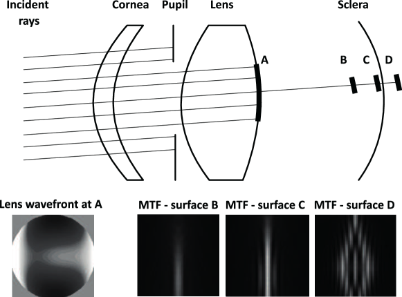
Figure 8: Computing the best-focus surfaces. A dense array of parallel, coherent rays (thin lines) is traced through the anterior optics (cornea, pupil, lens – medium lines) and the phase of the wavefront emerging through the posterior surface of the lens is fitted to Zernike polynomial functions. Bottom – Left: Example of a lens-emerging waveform. A Kirchhoff integral is applied to further propagate the wavefront and compute its modulation transfer function (MTF) on small surfaces perpendicular to the central ray. Bottom – Right: Example MTFs along probed surfaces. Surface C maximizes the Strehl ratio and hence corresponds to the best-focus surface for this wavelength. Computing the best-focus distance for a range of incidence angles (0-40 degrees), assuming axial symmetry, we reconstruct the best-focus surfaces for two wavelengths: $400\text{\,}\mathrm{nm}$ (blue) and $600\text{\,}\mathrm{nm}$ (red).

Appendix B Initial and boundary conditions

When considering a non-uniform scleral thickness, following Fatt1992 we prescribe

$$H(\Sigma)=\left\{\begin{array}[]{lr}0.65-0.2\tanh\left(\frac{\Sigma-0.167\pi R_{0}}{1.5}\right)\,,&x\in[0,0.5\pi R_{0}]\,,\\ 0.475+0.025\tanh(\Sigma-0.7\pi R_{0})\,,&x\in(0.5\pi R_{0},L]\,,\end{array}\right.$$ (27)

as shown in figure 9 alongside the initial fibre orientation, prescribed as

$$\frac{\psi({\Sigma})}{\pi}=0.25+\left\{\begin{array}[]{lr}0\,,&x\in[0,0.025\pi R_{0}]\,,\\ 0.06\cos\left(\frac{\Sigma-0.025\pi R_{0}}{0.1R_{0}}\right)-0.06\,,&x\in(0.025\pi R_{0},0.125\pi R_{0}]\,,\\ 0.15-0.17\cos\left(\frac{\Sigma-0.125\pi R_{0}}{0.375R_{0}}\right)\,,&x\in(0.125\pi R_{0},0.5\pi R_{0}]\,,\\ 0.22\cos\left(\frac{\pi(\Sigma-0.5\pi R_{0})}{L-0.5\pi R_{0}}\right)\,,&x\in(0.5\pi R_{0},L]\,,\end{array}\right.$$ (28)

following the observations of Girard2011 ; Grytz2014 .

\begin{overpic}[width=303.53267pt]{Figures/HandPsi/HandPsi.eps} \put(1.0,42.0){(a)} \put(51.0,42.0){(b)} \end{overpic}

Figure 9: Reference non-uniform scleral thickness and fibre orientation, shown in (a) and (b), respectively, from the works of Fatt1992 and Grytz2014 .

At the anterior point of the sclera, we match the scleral displacement to the inflation of a thin, spherically symmetric, non-growing shell of uniform thickness with no fibres, minimally modeling the cornea. Firstly, for this simple shell, we see that $\alpha_{s}^{c}=\alpha_{\phi}^{c}$, so for notational convenience we denote the stretch simply by $\alpha$, where the superscript on all other variables denotes that we are considering the cornea. Since the corneal reference configuration is spherical, we have

$$R^{c}=R_{0}^{c}\sin\left(\frac{\Sigma^{c}}{R_{0}^{c}}\right),$$ (29)

for $\Sigma^{c}\in[0,2\pi R_{0}^{c}]$, where $R_{0}^{c}$ is the radius of the sphere. The position of a point on the inflated sphere is thus given by

$$r^{c} =\alpha R_{0}^{c}\sin\left(\frac{\Sigma^{c}}{R_{0}^{c}}\right)\,,$$ (30a)

$$z^{c} =\alpha R_{0}^{c}\cos\left(\frac{\Sigma^{c}}{R_{0}^{c}}\right)+B\,,$$ (30b)

where $B$ is a constant of integration. The constraint of spherical symmetry ensures there is no normal shear force, $Q^{c}=0$, so that the shell deforms as a membrane. The solution to this problem is presented in Adkins1952 , where it is shown that

$$\Delta P=\frac{4C^{c}H^{c}}{\alpha R_{0}^{c}}\left(1-\frac{1}{\alpha^{6}}\right),$$ (31)

where $C^{c}$ is the neo-Hookean constant, $H^{c}$ is the undeformed thickness and $R_{0}^{c}$ is the undeformed radius of the shell. We take $C^{c}$, $H^{c}$ and $R_{0}^{c}$ to have values based on the mechanics of the cornea and we calculate $\alpha$ for the required pressure difference numerically, restricting $\alpha\in(1,7^{(1/6)})$ due to the non-injective relation between $\alpha$ and $\Delta P$. In particular, the upper limit here is the $\alpha$ value corresponding to the maximum of $1/\alpha-1/\alpha^{7}$ for $\alpha>1$, it placing a bound on the maximum pressure difference that we can consider, though we don’t vary the intraocular pressure in this work. Finally, evaluating the shape of the cornea at the point of attached to be sclera, we find the boundary conditions for the scleral shell to be

$$r^{\star} =\alpha R_{0}^{c}\sin\left(\frac{L}{R_{0}^{c}}\right),$$ (32a)

$$\theta^{\star} =\frac{L}{R_{0}^{c}},$$ (32b)

$$z^{\star} =\alpha R_{0}^{c}\left(1+\cos\left(\frac{L}{R_{0}^{c}}\right)\right).$$ (32c)

Appendix C Implementation

The governing equations presented in section 2.6 have a singularity when $r=0$, so we solve the system numerically on the truncated domain $\sigma\in[\sigma(\varepsilon,t),\sigma(L,t)]$ for $0<\varepsilon\ll 1$. By expanding the variables $r$, $\theta$, $\alpha_{s}$, $\kappa_{s}$ and $Q$ around $\sigma=0$ and evaluating at $\sigma=\sigma(\varepsilon,t)$, following Woolley2013 , then substituting the expansions into (21a,c,d,e) and equation 22 subject to equation 24, it becomes clear that the singularity is removable for compatible initial fibre directions. Indeed, isotropy is required as $\sigma\rightarrow 0$ because any preferred direction is undefined at the pole, and if we do not require $\psi\rightarrow\pi/4$ as $\sigma\rightarrow 0$ then there is a singularity in the stress as $\sigma\rightarrow 0$ in the fibre-reinforced shells. Intuitively, this is due to the preferred fibre orientation needing to change direction increasingly quickly as we approach the pole. In order to circumvent this in all the fibre-reinforced simulations in this work, we ensure that $\psi\rightarrow\pi/4$ as $\sigma\rightarrow 0$, subject to which the stress is finite and the boundary conditions on $r$ and $\theta$ can be replaced by the notationally cumbersome

$$r(\varepsilon) =\sigma(\varepsilon)\alpha_{s}(\sigma(\varepsilon)),$$ (33a)

$$\theta(\varepsilon) =\sigma(\varepsilon)\alpha_{s}(\sigma(\varepsilon))\kappa_{s}(\sigma(\varepsilon))\,,$$ (33b)

where we have suppressed the $t$-dependence of all quantities here for brevity. Now considering $Q$, we further manipulate equation 21 to admit the first integral

$$Q\cos\theta+rt_{s}\sin\theta-\frac{r^{2}\Delta P}{2}=A,$$ (34)

where $A$ is a constant. Since we require solutions that pass through $r=0$ with $\theta=\pi/2$, we find $A=0$. Thus, evaluating equation 34 at $\sigma=\sigma(\varepsilon,t)$ provides the analogous truncated boundary condition for $Q$. Note that whilst it is possible to use equation 34 to eliminate $Q$ from equations 21a, 21c, 21d, 21e and 22, preliminary numerical simulations suggested that it is easier to solve the five ordinary differential equations than the reduced system. Hence, we retain $Q$ in the governing equations and use equation 34 as a check on the numerical solutions.

We utilise MATLAB’s inbuilt adaptive boundary problem solver bvp4c to solve equations equations 21a, 21c, 21d, 21e and 22 subject to the boundary conditions truncated boundary conditions. The initial conditions are provided on a regular grid for $\Sigma\in[0,L]$ and growth is approximated with an explicit Euler scheme for equations 10 and 9. For each simulation, we ensure that the solution has converged with respect to our choices of grid size, timestep, truncation point and error tolerances in the solver. For example, the simulations in figure 3 were rerun on a refined spatial grid, with a smaller timestep, with a lower error tolerance in the bvp4c solver, and with a reduced truncation value $\varepsilon$. The largest relative errors in the variables $\kappa_{s}$, $\alpha_{s}$, $r$ and $\theta$ at $t=1$ in this refined simulation are $1.7\times 10^{-3}$, $2.1\times 10^{-5}$, $9.4\times 10^{-4}$ and $7.4\times 10^{-4}$ respectively, well below practical tolerance. Typical parameter values for the simulations in this work are given in table 1.

Name	Value	Source
$R_{0}$	$10\text{\,}\mathrm{mm}$	Gordon1985
$L$	$0.8\pi R_{0}$$\mathrm{mm}$	Gordon1985
$H$	$0.65\text{\,}\mathrm{mm}$	Based on equation 27
$\Delta P$	$2\text{\,}\mathrm{kPa}$	Oyster1999
$C$	$100\text{\,}\mathrm{kPa}$	Girard2009b
$D$	$100\text{\,}\mathrm{kPa}400\text{\,}\mathrm{kPa}$	Estimated
$E_{b}$	$18\text{\,}\mathrm{kPa}\text{\,}{\mathrm{mm}}^{3}$	Howell2009
$\eta_{0}$	$70\text{\,}{\mathrm{mm}}^{-1}$	Estimated
$\delta$	$4\text{\,}\mathrm{mm}12\text{\,}\mathrm{mm}$	Estimated
$\Gamma$	$2\text{\,}\mathrm{mm}6\text{\,}\mathrm{mm}$	Estimated

Table 1: Typical parameter values used in simulations, unless otherwise specified. $R_{0}$ and $L$ represent the size of a typical sclera towards the end of the rapid growth phase of development, at the beginning of the time interval that we model. The estimate for $C$ is based on values measured in monkey sclera, albeit with a slightly different constitutive law. The bending stiffness is estimated from $C$ and $H$ under the assumption of incompressibility. The corneal parameters $R_{0}^{c}$, $H^{c}$ and $C^{c}$ are chosen to match the scleral properties.

Appendix D Shell stresses

We briefly discuss the standard rationale for the functional form of the stresses specified by equations 17a and 17b. In a fully three-dimensional elastic body, the Cauchy stress, $\vec{\sigma}$, is

$$\vec{\sigma}=-p\mathbf{I}+2\mathbf{F}\frac{\partial W}{\partial\mathbf{C}}\mathbf{F}^{T}\,,$$ (35)

where $\mathbf{F}$ is the deformation gradient, $\mathbf{C}=\mathbf{F}^{T}\mathbf{F}$ is the right Cauchy-Green tensor, $p$ is the hydrostatic contribution to the stress associated with enforcing incompressibility, and $W$ is the strain-energy function. For a detailed account, we direct the interested reader to, for example, the work of Holzapfel2010 . If we suppose that $W=W(I_{1},I_{4},I_{6})$ where

$$I_{1} =tr\mathbf{C}\,,$$ (36a)

$$I_{4} =\mathbf{a}^{T}\mathbf{C}\mathbf{a}\,,$$ (36b)

$$I_{6} =\mathbf{b}^{T}\mathbf{C}\mathbf{b}\,,$$ (36c)

so that $I_{4}$ and $I_{6}$ represent the stretch of fibres that lie in the directions $\mathbf{a}$ and $\mathbf{b}$, then

$$\vec{\sigma}=-p\mathbf{I}+2\mathbf{F}\left(\frac{\partial W}{\partial I_{1}}\mathbf{I}+\frac{\partial W}{\partial I_{4}}\mathbf{a}\otimes\mathbf{a}+\frac{\partial W}{\partial I_{6}}\mathbf{b}\otimes\mathbf{b}\right)\mathbf{F}^{T}\,.$$ (37)

Furthermore, if we select the basis used for our scleral model so that $\mathbf{F}$ is diagonal with entries $\alpha_{s},\alpha_{\phi},\alpha_{n}$, define the fibre directions as in equations 12a, 12b and 13, so that $I_{4}=I_{6}$, and finally require $W(I_{1},I_{4},I_{6})=W(I_{1},I_{6},I_{4})$, then the off-diagonal terms in $\mathbf{a}\otimes\mathbf{a}$ and $\mathbf{b}\otimes\mathbf{b}$ cancel. Thus, the only non-zero components in equation 37 are

$$\sigma_{ss} =-p+2\alpha_{s}^{2}\frac{\partial W}{\partial I_{1}}+4\alpha_{s}^{2}\sin^{2}\psi\frac{\partial W}{\partial I_{4}}\,,$$ (38a)

$$\sigma_{\phi\phi} =-p+2\alpha_{\phi}^{2}\frac{\partial W}{\partial I_{1}}+4\alpha_{\phi}^{2}\cos^{2}\psi\frac{\partial W}{\partial I_{4}}\,,$$ (38b)

$$\sigma_{nn} =-p+2\alpha_{n}^{2}\frac{\partial W}{\partial I_{1}}\,.$$ (38c)

The shell’s thin geometry can be exploited as discussed in the context of membranes in Haughton2001 . We apply the key results in our shell model by working with resultant stresses of the form

$$t_{s} =\alpha_{n}H\sigma_{ss}\,,$$ (39a)

$$t_{\phi} =\alpha_{n}H\sigma_{\phi\phi}$$ (39b)

and setting $\sigma_{nn}=0$, often termed the ‘membrane assumption’. This is akin to noting that the curved shell is so thin that load across the surface due to the intraocular pressure is supported by in-shell tension, as opposed to stress across the shell thickness. The membrane assumption enables the elimination of the hydrostatic pressure, $p$, and our incompressibility assumption, $\alpha_{n}=1/\alpha_{s}\alpha_{\phi}$, gives principal in-shell stress resultants of the form equation 14.

References

- (1) Morgan, I.G., Ohno-Matsui, K., Saw, S.M.: Myopia. Lancet 379(9827), 1739–1748 (2012)
- (2) Spillmann, L.: Stopping the rise of myopia in Asia. Graefe’s Archive for Clinical and Experimental Ophthalmology 258(5), 943–959 (2020). DOI 10.1007/s00417-019-04555-0. URL http://link.springer.com/10.1007/s00417-019-04555-0
- (3) Sherwin, J.C., Mackey, D.A.: Update on the epidemiology and genetics of myopic refractive error. Expert Review of Ophthalmology 8(1), 63–87 (2013)
- (4) Dolgin, E.: The myopia boom. Nature 519(7543), 276–278 (2015)
- (5) Holden, B.A., Jong, M., Davis, S., Wilson, D., Fricke, T., Resnikoff, S.: Nearly 1 billion myopes at risk of myopia-related sight-threatening conditions by 2050 - time to act now. Clinical and Experimental Optometry 98(6), 491–493 (2015). DOI 10.1111/cxo.12339. URL http://doi.wiley.com/10.1111/cxo.12339
- (6) Holden, B.A., Fricke, T.R., Wilson, D.A., Jong, M., Naidoo, K.S., Sankaridurg, P., Wong, T.Y., Naduvilath, T.J., Resnikoff, S.: Global Prevalence of Myopia and High Myopia and Temporal Trends from 2000 through 2050. Ophthalmology 123(5), 1036–1042 (2016). DOI 10.1016/j.ophtha.2016.01.006. URL https://linkinghub.elsevier.com/retrieve/pii/S0161642016000257
- (7) Morgan, R., Speakman, J., Grimshaw, S.: Inuit myopia: an environmentally induced “epidemic”? Can. Med. Assoc. J. 112(5), 575 (1975)
- (8) Manjunath, V., Enyedi, L.: Pediatric myopic progression treatments: Science, sham, and promise. Current Ophthalmology Reports 2(4), 150–157 (2014)
- (9) Russo, A., Semeraro, F., Romano, M.R., Mastropasqua, R., Dell’Omo, R., Costagliola, C.: Myopia onset and progression: can it be prevented? Int. Ophthalmol. 34(3), 693–705 (2014)
- (10) Wu, P.C., Chuang, M.N., Choi, J., Chen, H., Wu, G., Ohno-Matsui, K., Jonas, J.B., Cheung, C.M.G.: Update in myopia and treatment strategy of atropine use in myopia control. Eye 33(1), 3–13 (2019). DOI 10.1038/s41433-018-0139-7
- (11) Fatt, I., Weissman, B.: Physiology of the eye: an introduction to the vegetative functions, 2nd edn. Butterworths London (1992)
- (12) Karimi, A., Razaghi, R., Navidbakhsh, M., Sera, T., Kudo, S.: Mechanical Properties of the Human Sclera Under Various Strain Rates: Elastic, Hyperelastic, and Viscoelastic Models. Journal of Biomaterials and Tissue Engineering 7(8), 686–695 (2017). DOI 10.1166/jbt.2017.1609. URL http://www.ingentaconnect.com/content/10.1166/jbt.2017.1609
- (13) Romano, M.R., Romano, V., Pandolfi, A., Costagliola, C., Angelillo, M.: On the use of uniaxial tests on the sclera to understand the difference between emmetropic and highly myopic eyes. Meccanica 52(3), 603–612 (2017). DOI 10.1007/s11012-016-0416-0. URL http://link.springer.com/10.1007/s11012-016-0416-0
- (14) Grytz, R., Girkin, C.A., Libertiaux, V., Downs, J.C.: Perspectives on biomechanical growth and remodeling mechanisms in glaucoma. Mech. Res. Commun. 42, 92–106 (2012)
- (15) Grytz, R., Fazio, M.A., Girard, M.J., Libertiaux, V., Bruno, L., Gardiner, S., Girkin, C.A., Downs, J.C.: Material properties of the posterior human sclera. J. Mech. Behav. Biomed. 29, 602–617 (2013)
- (16) Grytz, R., El Hamdaoui, M.: Multi-scale Modeling of Vision-Guided Remodeling and Age-Dependent Growth of the Tree Shrew Sclera During Eye Development and Lens-Induced Myopia. Journal of Elasticity 129(1-2), 171–195 (2017). DOI 10.1007/s10659-016-9603-4. URL http://dx.doi.org/10.1007/s10659-016-9603-4http://link.springer.com/10.1007/s10659-016-9603-4
- (17) Simonini, I., Pandolfi, A.: Customized Finite Element Modelling of the Human Cornea. PLOS ONE 10(6), e0130426 (2015). DOI 10.1371/journal.pone.0130426. URL https://dx.plos.org/10.1371/journal.pone.0130426
- (18) Sánchez, P., Moutsouris, K., Pandolfi, A.: Biomechanical and optical behavior of human corneas before and after photorefractive keratectomy. Journal of Cataract & Refractive Surgery 40(6), 905–917 (2014)
- (19) Pandolfi, A.: Cornea modelling. Eye and Vision 7(1), 1–15 (2020). DOI 10.1186/s40662-019-0166-x
- (20) Humphrey, J.D.: Cardiovascular solid mechanics. Cells, tissues, and organs. Springer Verlag, New York (2002)
- (21) Cowin, S.C.: Tissue growth and remodeling. Annu. Rev. Biomed. Eng. 6, 77–107 (2004)
- (22) Gasser, T.C., Ogden, R.W., Holzapfel, G.A.: Hyperelastic modelling of arterial layers with distributed collagen fibre orientations. J. R. Soc. Interface 3(6), 15–35 (2006)
- (23) Kuhl, E., Maas, R., Himpel, G., Menzel, A.: Computational modeling of arterial wall growth. Biomech. Model. Mechan. 6(5), 321–331 (2007)
- (24) Taber, L.A.: Biomechanics of growth, remodeling and morphogenesis. Appl. Mech. Rev. 48, 487–545 (1995)
- (25) Moulton, D.E., Goriely, A.: Possible role of differential growth in airway wall remodeling in asthma. J. Appl. Physiol. 110(4), 1003–1012 (2011)
- (26) Budday, S., Steinmann, P., Goriely, A., Kuhl, E.: Size and curvature regulate pattern selection in the mammalian brain. Extreme Mech. Lett. 4, 193–198 (2015)
- (27) Diether, S., Schaeffel, F.: Local changes in eye growth induced by imposed local refractive error despite active accommodation. Vision Res. 37(6), 659–668 (1997)
- (28) Wallman, J., Gottlieb, M.D., Rajaram, V., Fugate-Wentzek, L.A.: Local retinal regions control local eye growth and myopia. Science 237(4810), 73–77 (1987)
- (29) Foulds, W.S., Barathi, V.A., Luu, C.D.: Progressive myopia or hyperopia can be induced in chicks and reversed by manipulation of the chromaticity of ambient light. Invest. Ophth. Vis. Sci. 54(13), 8004–8012 (2013)
- (30) Kröger, R., Wagner, H.J.: The eye of the blue acara (aequidens pulcher, cichlidae) grows to compensate for defocus due to chromatic aberration. J. Comp. Physiol. A 179(6), 837–842 (1996)
- (31) Liu, R., Qian, Y.F., He, J.C., Hu, M., Zhou, X.T., Dai, J.H., Qu, X.M., Chu, R.Y.: Effects of different monochromatic lights on refractive development and eye growth in guinea pigs. Exp. Eye Res. 92(6), 447–453 (2011)
- (32) Werblin, F., Roska, B.: The movies in our eyes. Sci. Am. 296(4), 72–79 (2007)
- (33) Oyster, C.W.: The human eye. Sinauer Associates (1999)
- (34) Rodriguez, E.K., Hoger, A., McCulloch, A.D.: Stress-dependent finite growth in soft elastic tissues. J. Biomech. 27(4), 455–467 (1994)
- (35) Ambrosi, D., Ateshian, G., Arruda, E., Cowin, S., Dumais, J., Goriely, A., Holzapfel, G.A., Humphrey, J., Kemkemer, R., Kuhl, E., et al.: Perspectives on biological growth and remodeling. J. Mech. Phys. Solids 59(4), 863–883 (2011)
- (36) Kuhl, E.: Growing matter: A review of growth in living systems. J. Mech. Behav. Biomed. 29, 529–543 (2014)
- (37) Goriely, A.: The Mathematics and Mechanics of Biological Growth. Interdisciplinary Applied Mathematics. Springer New York (2017). URL https://books.google.co.uk/books?id=rgImDwAAQBAJ
- (38) Tongen, A., Goriely, A., Tabor, M.: Biomechanical model for appressorial design in magnaporthe grisea. J Theor. Biol. 240(1), 1–8. [We note there is a sign error in equation (8) corrected in Woolley et al. (2014)] (2006)
- (39) Woolley, T.E., Gaffney, E.A., Oliver, J.M., Baker, R.E., Waters, S.L., Goriely, A.: Cellular blebs: pressure-driven, axisymmetric, membrane protrusions. Biomech. Model. Mechan. 13(2), 463–476 (2014)
- (40) Coulombre, A.J.: The role of intraocular pressure in the development of the chick eye. i. control of eye size. Journal of Experimental Zoology 133(2), 211–225 (1956)
- (41) Maurice, D., Mushin, A.: Production of myopia in rabbits by raised body-temperature and increased intraocular pressure. The Lancet 288(7474), 1160–1162 (1966)
- (42) Quinn, G.E., Berlin, J.A., Young, T.L., Ziylan, S., Stone, R.A.: Association of intraocular pressure and myopia in children. Ophthalmology 102(2), 180–185 (1995)
- (43) Girard, M.J., Dahlmann-Noor, A., Rayapureddi, S., Bechara, J.A., Bertin, B.M., Jones, H., Albon, J., Khaw, P.T., Ethier, C.R.: Quantitative mapping of scleral fiber orientation in normal rat eyes. Investigative Ophthalmology & Visual Science 52(13), 9684–9693 (2011)
- (44) Jones, H., Girard, M., White, N., Fautsch, M.P., Morgan, J., Ethier, C., Albon, J.: Quantitative analysis of three-dimensional fibrillar collagen microstructure within the normal, aged and glaucomatous human optic nerve head. Journal of The Royal Society Interface 12(106), 20150066 (2015)
- (45) Gouget, C.L., Girard, M.J., Ethier, C.R.: A constrained von mises distribution to describe fiber organization in thin soft tissues. Biomechanics and modeling in mechanobiology 11(3-4), 475–482 (2012)
- (46) Coudrillier, B., Pijanka, J.K., Jefferys, J.L., Goel, A., Quigley, H.A., Boote, C., Nguyen, T.D.: Glaucoma-related changes in the mechanical properties and collagen micro-architecture of the human sclera. PloS one 10(7), e0131396 (2015)
- (47) Spencer, A.J.M.: Deformations of Fibre-Reinforced Materials. Oxford (1972)
- (48) Holzapfel, G.A., Ogden, R.W.: Constitutive modelling of arteries. Proc. R. Soc. A 466(2118), 1551–1597 (2010)
- (49) Melnik, A.V., Da Rocha, H.B., Goriely, A.: On the modeling of fiber dispersion in fiber-reinforced elastic materials. Int. J. Non Linear Mech. (2015)
- (50) Zhang, L., Albon, J., Jones, H., Gouget, C.L., Ethier, C.R., Goh, J.C., Girard, M.J.: Collagen microstructural factors influencing optic nerve head biomechanicscollagen microstructural factors. Investigative ophthalmology & visual science 56(3), 2031–2042 (2015)
- (51) Green, A.E., Adkins, J.E.: Large elastic deformations. Oxford University Press (1970)
- (52) Holzapfel, G.A., Ogden, R.W.: Constitutive modelling of arteries. P. R. Soc. A. 466(2118), 1551–1597 (2010)
- (53) Coudrillier, B., Boote, C., Quigley, H.A., Nguyen, T.D.: Scleral anisotropy and its effects on the mechanical response of the optic nerve head. Biomech Model Mechan 12(5), 941–963 (2013)
- (54) Girard, M., Downs, J.C., Bottlang, M., Burgoyne, C.F., Suh, J.F.: Peripapillary and posterior scleral mechanics, part II-experimental and inverse finite element characterization. J. Biomech. Eng. 131(5), 051012 (2009)
- (55) Wang, Y., Bensaid, N., Tiruveedhula, P., Ma, J., Ravikumar, S., Roorda, A.: Human foveal cone photoreceptor topography and its dependence on eye length. eLife 8, e47148 (2019). URL https://doi.org/10.7554/eLife.47148
- (56) Atchison, D.A.: Optical models for human myopic eyes. Vision Res. 46(14), 2236–2250 (2006)
- (57) Adkins, J.E., Rivlin, R.S.: Large elastic deformations of isotropic materials. IX. The deformation of thin shells. Philos. T. R. Soc. S.-A. 244(888), 505–531 (1952)
- (58) Gordon, R.A., Donzis, P.B.: Refractive development of the human eye. AMA Arch. Ophthalmol. 103(6), 785–789 (1985)
- (59) Howell, P., Kozyreff, G., Ockendon, J.: Applied solid mechanics. Cambridge University Press (2009)
- (60) Haughton, D.: Elastic membranes. London Mathematical Society Lecture Note Series pp. 233–267 (2001)