Super-resolution of periodic signals from short sequences of samples

Abstract

Reconstruction of undersampled periodic signals of unknown period is an important signal processing operation. It is especially difficult operation when the sequences of samples are short and no information on the inter-sequence time distances is given. For such a case, there exist some algorithms that allow for approximation of the sampled signal. However, these algorithms require either bandlimitedness of the signal, or noiseless samples. In this paper, we propose a novel algorithm which does not require the signal to be bandlimited and it can cope with additive noise in the samples. The algorithm is illustrated and validated with real data.

Index Terms—  signal reconstruction, signal sampling, nonuniform sampling, point cloud approximation

1 Introduction

Periodic signal reconstruction from a finite sequence of samples (a sample train) taken at a given sampling rate is an important signal processing operation needed in many applications in diverse areas such as communications, remote sensing, system testing, and characterization. If the period $T$ of the sampled signal is known and the signal is band-limited, then a single sample train allows for perfect reconstruction of the signal, provided that the train is long enough [1, 2, 3]. In such a case, the reconstruction reduces to solving a set of linear equations. If period $T$ is not known but the sampling period $\tau$ is much smaller than $T$, then one can get a reasonable approximation to the sampled signal by interpolation. This is how the digital scopes usually reconstruct the sampled signals. The situation becomes much more complicated when $\tau$ and $T$ are of the same order of magnitude. In such a case, we deal with undersampled signals and the methods of dealing with approximation in this case are often called super-resolution methods. Undersampling might be due purely economic reasons, since high-speed sampling systems are relatively expensive, or it can result from systems designed or configured for a low frequency application to recover unanticipated high frequency signals [4]. The simplest super-resolution technique is based on the stroboscopic effect. To take advantage of this effect, one needs to get a precise estimate of period $T$. This crucial estimation is usually performed in the time domain [4, 5, 6, 7] or in the frequency domain [8]. In both the approaches, a long train of samples is required to get a reasonable period estimate. If the nature of the sampling process or the sampling hardware allows for acquisition of short sample-trains only, then one can still achieve super-resolution by using multiple such trains, even if the inter-train time distances are not known. This is possible if the sampled signal is of known band limit [9, 10], or if the starting times of the trains are distributed uniformly (in the probabilistic sense) when considered modulo $T$ [11, 12], or if the ratio $\tau/T$ is irrational [13]. The algorithms for signal reconstruction proposed by the author in [11, 12] require noiseless samples. In this paper we propose an algorithm which can deal with trains of noisy samples. The algorithm is based on the ideas introduced in [11].

The next section explains the relationship between periodic signals and the probability distribution of sample trains. Section 3 proposes an algorithm for reconstruction of periodic signals from a finite number of trains of noisy samples. In Section 4, we present the results of a proof-of-concept experiment which was designed for the proposed algorithm verification. The paper is concluded in Section 5.

2 Distribution of trains of samples

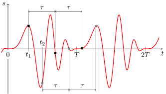
Fig. 1: A $T$-periodic signal and its two sample trains of length $3$ taken with sampling period $\tau\approx 0.4T$ (the sequences start at $t_{1}$ and $t_{2}$, respectively)

A train of samples of signal $s$ is henceforth denoted by $\mathbf{s}_{d,\tau}(t)$, i.e.,

$$\mathbf{s}_{d,\tau}(t)=[s(t),\,s(t+\tau),\,\dots,\,s(t+(d-1)\tau)]\in\mathbf{R}^{d}.$$ (1)

where $d$ is the length of the train, $t$ is its starting time, and $\tau$ is the inter-sample distance (sampling period). Fig. 1 shows an example of a periodic signal and its 3-sample trains.

If $s$ is a continuous periodic function of variable $t$, then so is the above mapping $\mathbf{s}_{d,\tau}$. In this case, the image of $\mathbf{s}_{d,\tau}$ is a closed curve. If we treat time instant $t$ in (1) as a random variable distributed uniformly on the interval $[0,T)$, then the resulting vector $\mathbf{s}_{d,\tau}(t)$ becomes a multivariate $\mathcal{C}$-valued random variable henceforth denoted by $\mathcal{S}_{d,\tau}$. In [11] it is shown that the probability distribution of $\mathcal{S}_{d,\tau}$ determines signal $s$ up to a time shift provided that: function $\mathbf{s}_{d,\tau}$ restricted to the interval $[0,T)$ is a one-to-one mapping, the time derivative of $\mathbf{s}_{d,\tau}$ does not vanish anywhere, and $\tau<\frac{T}{2}$. For the completeness of this paper we rephrase the reconstruction algorithm presented in [11] as Algorithm 1. There and henceforth, $f_{\mathcal{C}}$ is the probability density function (PDF) of $\mathcal{S}_{d,\tau}$, $\mathcal{C}$ is the closed curve formed by the trains of samples, i.e., $\mathcal{C}$ is the image of function $\mathbf{s}_{d,\tau}$, $L$ is the length of $\mathcal{C}$, $\pi_{m}$ is the projection onto the $m$-th coordinate, i.e., $\pi_{m}([x_{1},\dots,x_{d}])=x_{m}$, $f\circ g$ means a composition of the functions, i.e, $f\circ g(t)=f(g(t))$, and $f\stackrel{{\scriptstyle\phi}}{{=}}g$ means that functions $f$ and $g$ are equal up to a time shift, i.e., there exists $t_{0}$ such that $f(t)=g(t+t_{0})$ for all $t\in\mathbf{R}$.

Algorithm 1 Signal reconstruction from the probability distribution of its trains of samples (noiseless case) [11]

Input: sampling period $\tau$, PDF $f_{\mathcal{C}}$ and its support $\mathcal{C}$

Output: signal $s$ (up to a time shift), and its period $T$.

1. Take any arc-length parametrization of curve $\mathcal{C}$ and extend it to an $L$-periodic function $\mathbf{q}_{1}\colon\mathbf{R}\to\mathcal{C}$.

2. Set $\mathbf{q}=\mathbf{q}_{1}\circ r$, where function $r\colon\mathbf{R}\to\mathbf{R}$ is given by equation $x=\int_{0}^{Lr(x)}f_{\mathcal{C}}(\mathbf{q}_{1}(u))\mathrm{d}u.$

3. Take any integers $1\leq k<l\leq d$ and find $x_{0}\in(0,1)$ such that

   $$\pi_{k}\circ\mathbf{q}\left(x+\left(l-k\right)x_{0}\right)=\pi_{l}\circ\mathbf{q}\left(x\right)\quad\forall x\in\mathbf{R}.$$ (2)

4. If $x_{0}<\frac{1}{2}$, then $T=\frac{\tau}{x_{0}}$ and $\mathbf{s}_{d,\tau}(t)\stackrel{{\scriptstyle\phi}}{{=}}\mathbf{q}(\frac{t}{T})$.

   If $x_{0}>\frac{1}{2}$, then $T=\frac{\tau}{1-x_{0}}$ and $\mathbf{s}_{d,\tau}(t)\stackrel{{\scriptstyle\phi}}{{=}}\mathbf{q}(\frac{-t}{T})$.

5. $s(t)\stackrel{{\scriptstyle\phi}}{{=}}\sum_{k=1}^{d}\pi_{k}\circ\mathbf{s}_{d,\tau}\bigl{(}t+(k-1)\tau\bigr{)}.$

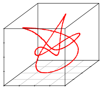
Fig. 2: A point cloud formed by a large number of noisy $3$-sample sequences of the signal presented in Fig. 1 (for bounded noise the points lie inside a pipe of a bounded diameter; in the absence of the noise the points would form a closed curve)

We model the additive noise in the samples by assuming that acquired trains of samples are of the form:

$$\mathbf{s}_{d,\tau}(t)+\mathbf{\eta}\in\mathbf{R}^{d},$$ (3)

where $t$ is a random variable distributed uniformly in the interval $[0,T)$, and $\mathbf{\eta}$ is a $d$-variate random variable with finite variance $\sigma^{2}$ and with radial PDF $f_{\sigma}$, i.e.,

$$f_{\sigma}(\mathbf{x})=c_{d}\sigma^{-d}f_{1}\left(\|\mathbf{x}\|/\sigma\right),$$ (4)

where $\|\mathbf{x}\|$ denotes the Euclidean norm of $\mathbf{x}$, and where $f_{1}$ is the PDF of a unit variance positive random variable. Noisy trains (3) no longer lie in a closed curve $\mathcal{C}$ because the noise scatters these points around that curve. However, if the noise variance is small, the noisy trains fall into a small neighborhood of $\mathcal{C}$, i.e., curve $\mathcal{C}$ forms a thread along which the probability distribution of noisy trains (3) is concentrated. Fig. 2 illustrates such a situation by showing a cloud of trains of noisy samples of the periodic signal presented in Fig. 1.

Let $f$ denote the PDF of noisy trains (3). Function $f$ is a convolution of functions $f_{\mathcal{C}}$ and $f_{\sigma}$, i.e.,

$$f(\mathbf{p})=\int_{\mathcal{C}}f_{\mathcal{C}}(\mathbf{q})f_{\sigma}(\mathbf{p}-\mathbf{q})\mathrm{d}\mathbf{q}.$$ (5)

Therefore, if $\sigma$ is small, then for each point $\mathbf{p}\in\mathcal{C}$

$$f(\mathbf{p})\approx c_{d}\sigma^{-(d-1)}f_{\mathcal{C}}(\mathbf{p}).$$ (6)

Indeed, we can split the integral in (5) into two parts: the integral over a $\sqrt{\sigma}$-neighborhood of $\mathbf{p}$, and over the rest of curve $\mathcal{C}$, respectively. When $\sigma$ tends to $0$, the former integral becomes the right hand side of (6), while the latter integral is bounded by $\sigma^{-(d-1)}h(\sigma)$, where $h(\sigma)$ is proportional to $\int_{1/\sqrt{\sigma}}^{\infty}f_{1}(y)\mathrm{d}y\stackrel{{\scriptstyle\sigma\to 0}}{{\to}}0$. Thus, the smaller the variance of $\mathbf{\eta}$ is, the more accurate approximation (6) is.

3 The reconstruction algorithm

The trains of samples used for the reconstruction of a signal are henceforth treated as points in a $d$-dimensional space and they are denoted by

$$\mathbf{p}_{1},\dots,\mathbf{p}_{n}\in\mathbf{R}^{d}.$$ (7)

The outline of the proposed reconstruction algorithm is presented below as Algorithm 2. The following subsections explain in detail the three stages of the outline.

Algorithm 2 Signal reconstruction from a finite number of trains of noisy samples (outline)

Input: sampling period $\tau$, trains of samples (7)

Output: estimates $\hat{s}$ and $\hat{T}$ of signal $s$ and its period $T$, resp.

1. Approximate points (7) with a closed smooth curve $\hat{\mathcal{C}}$,

2. Estimate a PDF $\hat{f_{\mathcal{C}}}$ along curve $\hat{\mathcal{C}}$ with a help of (6),

3. Compute $\hat{s}$ and $\hat{T}$ as the output of appropriately adapted Algorithm 1 applied to: $\tau$, $\hat{f_{\mathcal{C}}}$, $\hat{\mathcal{C}}$

3.1 Curve $\mathcal{C}$ approximation

The problem of recovering a curve from its noisy samples (cloud of points) appears in several applications such as Computed Axial Tomography, Coordinate-Measuring Machine measurements and Magnetic Resonance Imaging. There exist various strategies to solve this problem. They are based on methods of mathematical analysis [14, 15], geometry [16, 17] and statistics [18, 19, 20, 21]. The approximation algorithm presented in [21] is especially well suited for the first stage of Algorithm 2 because it can cope with closed curves, it works in Euclidean space of arbitrary dimension, and it is relatively simple. The algorithm of [21] has a parameter $R$ which can be adjusted for a given or expected noise variance. The output of the algorithm of [21] comprises sequences of points, where each sequence represents the nodes of a polygonal chain which approximate a curve. If the first and the last points of an output sequence coincide, then the corresponding polygonal chain represents a closed curve. An output sequence which does not represent a closed curve, as well as more than one output sequences, signals that either the algorithm parameter $R$ is too big, or the number of points $n$ is not big enough, or eventually that the underlying curve has some self-intersections. If the algorithm of [21] produces only one output sequence

$$\tilde{\mathbf{p}}_{1},\dots,\tilde{\mathbf{p}}_{M}\in\mathbf{R}^{d},$$ (8)

and if this sequence represents a closed polygonal path, i.e., $\tilde{\mathbf{p}}_{M}=\tilde{\mathbf{p}}_{1}$, then what remains to complete the first stage of Algorithm 2 is to interpolate the nodes of the path with a smooth curve. This can be achieved with periodic cubic splines [22]. For the needs of the next subsection, we denote the resulting smooth curve parametrization by $\hat{\mathbf{q}}_{1}\colon[0,\hat{L})\to\mathbf{R}^{d}$. Without loss of generality, we henceforth assume that $\hat{\mathbf{q}}_{1}(0)=\tilde{\mathbf{p}}_{1}$ and that $\hat{\mathbf{q}}_{1}$ is already an arc-length parametrization, i.e. $\|\hat{\mathbf{q}}^{\prime}_{1}\|=1$ and $\hat{L}$ is the length of curve $\hat{\mathcal{C}}$ which is the image of $\hat{\mathbf{q}}_{1}$.

3.2 Density estimation

Let $\tilde{t}_{1},\dots,\tilde{t}_{M}$ denote the preimages of points (8) under $\hat{\mathbf{q}}_{1}$, i.e.,

$$\hat{\mathbf{q}}_{1}(\tilde{t}_{i})=\tilde{\mathbf{p}}_{i},\quad i=1,\dots,M.$$ (9)

In order to estimate density along curve $\hat{\mathcal{C}}$, for each point $\tilde{t}_{i}$ we compute the number $c_{i}$ of points (7) that lie in the $R$-neighborhood of $\tilde{\mathbf{p}}_{i}$, where $R$ is the same as described in the previous subsection. We obtain $\hat{f_{\mathcal{C}}}$ by linear interpolation of values $c_{i}$ followed by division of the resulting function by a factor which makes the interpolation function a PDF, i.e., by a factor which makes the integral of the so obtained estimate $\hat{f_{\mathcal{C}}}$ unitary. This factor can be expressed as

$$\sum_{i=1}^{M-1}\left(\tilde{t}_{i+1}-\tilde{t}_{i}\right)\frac{c_{i}+c_{i+1}}{2}.$$ (10)

3.3 Signal reconstruction

In the final stage of Algorithm 2 we refer to Algorithm 1. However, Algorithm 1 has to be adapted for the fact that $\hat{f_{\mathcal{C}}}$ and $\hat{\mathbf{q}}$ are estimates only and they could make Equations (2) not solvable for any $1\leq k<l\leq d$. Therefore, we look for a least-squares solutions to the set of Equations (2), i.e., we find $x_{0}$ by minimizing a functional $F$ in the interval $(0,1)$, where

$$F(x_{0})=\\ \sum_{1\leq k<l\leq d}\int_{0}^{1}\left(\pi_{k}\left(\mathbf{q}\left(x+(l\!-\!k)x_{0}\right)\right)-\pi_{l}\left(\mathbf{q}\left(x\right)\right)\right)^{2}\mathrm{d}x.$$ (11)

4 Proof of concept experiments

To verify the proposed algorithm, we have designed the following experiments. A chirp-like $T$-periodic signal presented in Fig. 1 was generated with a function generator and recorded with a digital scope. The sampling period $\tau$ of the scope was set to around $0.39T$. The signal peak-to-peak value was around $4\text{\,}\mathrm{V}$ and the quantization step of the scope was $\Delta=$0.02\text{\,}\mathrm{V}$$ (we may assume that the noise standard deviation $\sigma$ is of the same order of magnitude). For a fixed value of sample train length $d$ and a fixed number $n$, we picked at random $n$ $d$-sample trains from the long sample sequence recorded with the scope. These sequences, treated as points (7), and the sampling period $\tau$ made up the input data for Algorithm 2, in which we set $R=5\Delta$ (the parameter is needed at the first two stages of the algorithm). The reconstructed signal period $\hat{T}$ and signal $\hat{s}$ were then compared to known period $T$ and a reference signal $s_{\text{ref}}$, respectively. The reference signal was obtained by recording the averaged (by the scope) signal with the same digital scope, but with the sampling period set to $\tau_{\text{ref}}<\tau/1000$.

Fig. 3: Signal reconstruction root-mean-square errors (13)

To assess the quality of reconstruction, the following reconstruction error measures were computed:

$$\epsilon_{T} =|T-\hat{T}|,$$ (12)

$$\epsilon_{2} =\min_{t_{0}\in[0,T)}\sqrt{\int_{0}^{T}\left(s_{\text{ref}}(t-t_{0})-\hat{s}(t\hat{T}/T)\right)^{2}},$$ (13)

$$\epsilon_{\infty} =\min_{t_{0}\in[0,T)}\max_{t\in[0,T)}|s_{\text{ref}}(t-t_{0})-\hat{s}(t\hat{T}/T)|.$$ (14)

(the argument of the reconstructed signal $\hat{s}$ in (13) and (14) is scaled to compare two periodic signals of the same period). For each pair of the considered values of parameters $d$ and $n$, the experiment was repeated $100$ times. The resulting errors are presented as box-plots in Fig. 3–5. The figures show that for the signal considered in the experiment, the super-resolution signal reconstruction has been achieved. The period estimate error is by three order of magnitude lower than the sampling period $\tau$. The both root-mean-square and maximum errors of signal reconstructions reach the level of the quantization step $\Delta$ of the recording of the reference signal. Not surprisingly, the experiment showed that the quality of signal reconstruction rises with the amount of input data. The reason for this is two-fold. First, the number of cloud points affects the quality of curve reconstruction from that cloud (the first stage of the algorithm). A quantitative study of this phenomenon and the role of the dimension of the space and the amplitude of the noise in the process of curve reconstruction from a point cloud can be found in [21]. Second, the amount of input data affects the density estimation along the reconstructed curve. We expect that the root-mean-square error of such estimation is similar to that based on histogram, i.e., it falls at rate $n^{-1/3}$ [23].

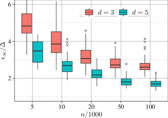
Fig. 4: Signal reconstruction maximum errors (14)

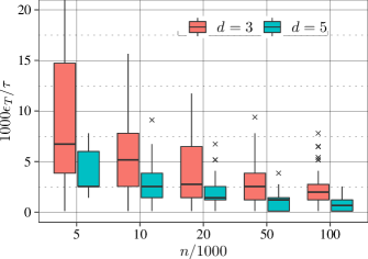
Fig. 5: Period estimation errors (12)

5 Conclusion

We have proposed an algorithm for signal reconstruction from the short trains of noisy samples of the signal. The algorithm allows for achieving a super-resolution reconstruction as it allows the sampling period $\tau$ to be relatively big with respect to the signal period $T$ (the algorithm requires only $\tau<\frac{1}{2}T$). We performed a series of experiments, which showed that the reconstructed signal is close to the reference signal and that the larger the number of trains is, the smaller reconstruction errors are obtained. We believe that the ability of the algorithm to cope with noisy and non-continuous recordings (multiple trains of samples) will make it a valuable tool in a number of applications.

References

- [1] T. Schanze, “Sinc interpolation of discrete periodic signals,” IEEE Transactions on Signal Processing, vol. 43, no. 6, pp. 1502–1503, Jun 1995.
- [2] F. Candocia and J. C. Principe, “Comments on sinc interpolation of discrete periodic signals,” IEEE Transactions on Signal Processing, vol. 46, no. 7, pp. 2044–2047, Jul 1998.
- [3] S. R. Dooley and A. K. Nandi, “Notes on the interpolation of discrete periodic signals using sinc function related approaches,” IEEE Transactions on Signal Processing, vol. 48, no. 4, pp. 1201–1203, Apr 2000.
- [4] C. Rader, “Recovery of undersampled periodic waveforms,” IEEE Transactions on Acoustics, Speech, and Signal Processing, vol. 25, no. 3, pp. 242–249, Jun 1977.
- [5] A. J. Silva, “Reconstruction of undersampled periodic signals,” NASA STI/Recon Technical Report N, vol. 87, Jan. 1986.
- [6] D. Bhatta, J. W. Wells, and A. Chatterjee, “Time domain characterization and test of high speed signals using incoherent sub-sampling,” in 2011 Asian Test Symposium, Nov 2011, pp. 21–26.
- [7] N. Tzou, D. Bhatta, S. W. Hsiao, H. W. Choi, and A. Chatterjee, “Low-cost wideband periodic signal reconstruction using incoherent undersampling and back-end cost optimization,” in 2012 IEEE International Test Conference, Nov 2012, pp. 1–10.
- [8] H. Choi, A. V. Gomes, and A. Chatterjee, “Signal acquisition of high-speed periodic signals using incoherent sub-sampling and back-end signal reconstruction algorithms,” IEEE Transactions on Very Large Scale Integration (VLSI) Systems, vol. 19, no. 7, pp. 1125–1135, Jul 2011.
- [9] P. Vandewalle, L. Sbaiz, J. Vandewalle, and M. Vetterli, “How to take advantage of aliasing in bandlimited signals,” in 2004 IEEE International Conference on Acoustics, Speech, and Signal Processing, May 2004, vol. 3, pp. iii–948–51 vol.3.
- [10] P. Vandewalle, L. Sbaiz, J. Vandewalle, and M. Vetterli, “Super-resolution from unregistered and totally aliased signals using subspace methods,” IEEE Transactions on Signal Processing, vol. 55, no. 7, pp. 3687–3703, July 2007.
- [11] M. W. Rupniewski, “Triggerless random interleaved sampling,” in ICASSP 2020 - 2020 IEEE International Conference on Acoustics, Speech and Signal Processing (ICASSP), 2020, pp. 5605–5609.
- [12] M. W. Rupniewski, “Reconstruction of periodic signals from asynchronous trains of samples,” IEEE Signal Processing Letters, vol. 28, pp. 289–293, 2021.
- [13] M. W. Rupniewski, “Period and signal reconstruction from the curve of sample-sequences,” arXiv e-prints, p. arXiv:2008.08832, Aug 2020.
- [14] L. Fang and D. C. Gossard, “Multidimensional curve fitting to unorganized data points by nonlinear minimization,” Computer-Aided Design, vol. 27, no. 1, pp. 48 – 58, 1995.
- [15] A. A. Goshtasby, “Grouping and parameterizing irregularly spaced points for curve fitting,” ACM Transactions on Graphics, vol. 19, no. 3, pp. 185–203, 2000.
- [16] H. Pottmann and T. Randrup, “Rotational and helical surface approximation for reverse engineering,” Computing (Vienna/New York), vol. 60, no. 4, pp. 307–322, 1998.
- [17] S.-W. Cheng, S. Funke, M. Golin, P Kumar, S.-H. Poon, and E. Ramos, “Curve reconstruction from noisy samples,” Computational Geometry, vol. 31, no. 1–2, pp. 63 – 100, 2005.
- [18] T. Hastie and W. Stuetzle, “Principal curves,” Journal of the American Statistical Association, vol. 84, no. 406, pp. 502–516, 1989.
- [19] D. Levin, “The approximation power of moving least-squares,” Mathematics of Computation, vol. 67, no. 224, pp. 1517–1531, 1998.
- [20] I.-K. Lee, “Curve reconstruction from unorganized points,” Computer Aided Geometric Design, vol. 17, no. 2, pp. 161–177, 2000.
- [21] M. W. Rupniewski, “Curve reconstruction from noisy and unordered samples,” in ICPRAM 2014 - Proceedings of the 3rd International Conference on Pattern Recognition Applications and Methods, 2014, pp. 183–188.
- [22] R. H. Bartels, J. C. Beatty, and B. A. Barsky, An Introduction to Splines for Use in Computer Graphics and Geometric Modeling, Morgan Kaufmann Publishers Inc., San Francisco, CA, USA, 1987.
- [23] L. Wasserman, All of Statistics: A Concise Course in Statistical Inference, Springer Publishing Company, Incorporated, 2010.