Quantile Bandits for Best Arms Identification

Abstract

We consider a variant of the best arm identification task in stochastic multi-armed bandits. Motivated by risk-averse decision-making problems, our goal is to identify a set of $m$ arms with the highest $\tau$-quantile values within a fixed budget. We prove asymmetric two-sided concentration inequalities for order statistics and quantiles of random variables that have non-decreasing hazard rate, which may be of independent interest. With these inequalities, we analyse a quantile version of Successive Accepts and Rejects (Q-SAR). We derive an upper bound for the probability of arm misidentification, the first justification of a quantile based algorithm for fixed budget multiple best arms identification. We show illustrative experiments for best arm identification.

1 Introduction

Multi-Armed Bandits (MAB) are sequential experimental design problems where an agent adaptively chooses one (or multiple) option(s) among a set of choices based on certain policies. We refer to “options” as “arms” in MAB problems. In contrast with full feedback online decision-making problems where sample rewards for all arms are fully observable to agents in each round, in MAB tasks the agent only observes the sample reward from the selected arm in each round, with no information about other arms.

One of the key steps in the theoretical analysis for bandit algorithms is concentration inequalities, which provides bounds on how a random variable deviates from some statistical summary (typically its expected value). Inspired by the approach in Boucheron & Thomas (2012), we propose in Section 2 new concentration inequalities for order statistics and quantiles of distributions with non-decreasing hazard rates (Definition 1). Previous work derived concentration bounds of quantiles via the empirical cumulative distribution function (c.d.f.). Our proof uses a new approach based on the extended Exponential Efron-Stein inequality (Theorem 3), and non-trivially extends the concentration of order statistics (Boucheron & Thomas, 2012). Our proposed concentration inequality can be useful for various applications, for example, the multi-armed bandits problem as illustrated in this work, learning theory, A/B-testing (Howard & Ramdas, 2019), and model selection (Massart, 2000).

	Mean	0.5-Quantile		Mean	0.8-Quantile
A	3.50	3.50	C	1.45	2.33
B	4.00	2.80	D	2.50	4.00
OptArm	B	A	Gap	1.05	1.67

Table 1: Summary statistics for toy example rewards

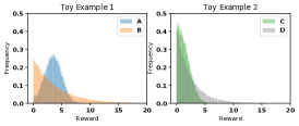
Figure 1: Toy example reward histograms.

We apply the proposed concentration inequality to the Best Arm Identification (BAI) task with fixed budget (Audibert et al., 2010; Bubeck et al., 2013). The goal of BAI is to select the best arm (in our case the top $m\geq 1$ arms) after the exploration phase (i.e. budget has run out). The agent can explore the environment and perform actions during the exploration phase without penalty. In contrast to the majority of previous work which identifies optimal arms by summarising a distribution by its mean, we address risk-averse bandits by evaluating the quality of arms by a quantile value of the reward distribution. We consider the bandit problem of quantile based $m$ best arms identification, where the goal is to identify a set of $m$ arms with the highest $\tau$-quantile values. To the best of our knowledge, existing quantile work focuses on single optimal arm identification, and we are the first work that addresses multiple best arms identification for fixed budget setting with respect to the $\tau$-quantile. Our proposed algorithm is in Section 4.

Studying quantile concentrations and identifying arms with optimal quantiles have been shown to be beneficial for many cases, such as when the rewards are qualitative (Szörényi et al., 2015), when the decision-making is risk-averse (Yu & Nikolova, 2013; David et al., 2018), when the rewards contain outliers (Altschuler et al., 2019), or when the reward distributions are highly skewed (Howard & Ramdas, 2019).

We motivate the use of quantiles as summary statistics with two toy examples, with simulated reward histograms of 2 arms shown in Figure 1 and corresponding summary statistics shown in Table 1. The first example illustrates when risk-averse agents should prefer quantiles. Consider a vaccine testing problem (Cunningham et al., 2016), where the goal is to identify the most reliable vaccine after the exploration phase. The reward is the efficacy of the vaccine. Risk-averse agents tend to exclude vaccine candidates which return a large number of small rewards even though they may have a larger expected value (e.g. B in Figure 1). In such case, a policy guided by a fixed level of quantiles (e.g. 0.5-quantile, the median) will choose a less risky arm (i.e. one with less low rewards). The second example shows when the distributions are skewed, the quantile can provide a bigger gap between arms, which turns out to produce a smaller probability of error (Definition 2). As shown by toy example 2 in Figure 1, the quantile and mean reflect the same preference, but the difference between arms is larger for the 0.8-quantile. The choice of quantile level $\tau$ provides an extra degree of modelling freedom, that the practitioner may use to capture domain requirements or to achieve a smaller error probability.

Our contributions are: (i) Two-sided exponential concentration inequalities for order statistics of rank $k$ (w.r.t its expectation) for a general family (with non-decreasing hazard rate) of random variables. (ii) Two-sided exponential concentration inequalities for estimations of $\tau$-quantile (w.r.t. population quantile) based on our results on order statistics. (iii) The first $\tau$-quantile based multiple ($m\geq 1$) arms identification algorithm (Q-SAR) for the fixed budget setting. (iv) Theoretical analysis for the proposed Q-SAR algorithm, showing an exponential rate upper bound on the probability of error. (v) Empirical illustrations for the Q-SAR algorithm, which indicates that Q-SAR outperforms baseline algorithms for the best arms identifications task.

2 Concentration Inequalities

In this section, we show our results for concentration inequalities on order statistics and quantiles. We apply these results to prove error bounds for bandits in Section 4. Order statistics have been used and studied in various areas, such as robust statistics and extreme value theory. The non-asymptotic convergence analysis for order statistics provides a way to understand the probability of order statistics deviates from its expectation, and it is useful to support the decision-making with limited samples under uncertainty.

Let $\{X_{t}\}_{t=1}^{n}$ be $n$ i.i.d samples drawn from the distribution of $X$, and let the $\{X_{(t)}\}_{t=1}^{n}$ be the order statistics of $\{X_{t}\}_{t=1}^{n}$ written in decreasing order, i.e.

$$X_{(1)}\geq X_{(2)}\cdots\geq X_{(n)}.$$ (1)

We call $X_{(k)}$ the $k$ rank order statistic, and $X_{(1)}$ and $X_{(n)}$ the maximum and minimum respectively. Denote the (left-continuous) quantile with $\tau\in(0,1)$ of a random variable $X$ by

$$Q^{\tau}(X):=\inf\{x:\mathbb{P}(X\leq x)\geq\tau\}.$$ (2)

We will refer $Q^{\tau}(X)$ as $Q^{\tau}$ whenever $X$ is clear from the context. With the empirical c.d.f. defined as $\hat{F}_{n}(x)=\frac{1}{n}\sum_{s=1}^{n}\mathbb{I}\{X_{s}\leq x\}$, the empirical $\tau$-quantile with $n$ samples is defined as

$$\hat{Q}^{\tau}_{n}:=\inf\{x:\hat{F}_{n}(x)\geq\tau\}=X_{(\lfloor n(1-\tau)\rfloor)}.$$ (3)

2.1 Problem Setting

We now introduce the family of reward distributions we consider in this work. We consider continuous non-negative reward random variables $X$ with p.d.f. $f$ and c.d.f. $F$ which satisfy Assumption 1. Note that we are considering distributions that are unbounded on the right.

Definition 1 (Hazard rate).

The hazard rate of a random variable $X$ evaluated at the point $x$ is defined as (assuming density $f(x)$ exists)

$$h(x) :=\lim_{\theta\rightarrow 0}\frac{\mathbb{P}\left(x\leq X\leq x+\theta|X\geq x\right)}{\theta}=\frac{f\left(x\right)}{1-F\left(x\right)}.$$

Assumption 1 (IHR).

We consider reward distributions with non-negative support $[0,\infty)$ having non-decreasing hazard rate (IHR), i.e. for all $x_{1}\geq x_{2}\geq 0$, the hazard rate satisfies $h(x_{1})\geq h(x_{2})$. We further suppose that the lower bound of the hazard rate $L:=\inf_{x}h(x)>0$.

The IHR assumption is useful in survival analysis. If the hazard rate $h(x)$ increases as $x$ increases, $\mathbb{P}\left(x\leq X\leq x+\theta|X\geq x\right)$ will increase as well. For example, a man is more likely to die within the next month when he is 88 years old than when he is 18 years old. Common examples of IHR distributions include the absolute Gaussian, exponential, and Gumbel distributions. Log-concave distributions are IHR and have widely been applied to economics, search theory, monopoly theory (Bagnoli & Bergstrom, 2005).

In the following sections, we show our main results about the concentration bounds for order statistics and quantiles, and details are provided in Appendix B.

2.2 Order Statistics

Our goal is to derive two exponential rate concentration bounds in terms of rank $k$ order statistics out of $n$ samples. A roadmap of the technical derivations needed is deferred to Section 3, and we present only the lemmas needed for analysing BAI in this section. For $\gamma\geq 0$, the right and left tail are respectively,

$$\mathbb{P}\left(X_{(k)}-\mathbb{E}[X_{(k)}]\geq d^{r}_{k,\gamma}\right)\leq\exp(-\gamma),$$ (4)

$$\mathbb{P}\left(\mathbb{E}[X_{(k)}]-X_{(k)}\geq d^{l}_{k,\gamma}\right)\leq\exp(-\gamma).$$ (5)

where $d^{r}_{k,\gamma},d^{l}_{k,\gamma}$ are the right and left confidence intervals.

To derive such bounds, we consider the entropy method and the Cramér-Chernoff method (Boucheron et al., 2013). These results are used to derive the following lemmas for deviation of order statistics. Recall $L$ is the lower bound of the hazard rate, $k$ is chosen from the positive integers $\mathbb{N}^{\ast}$.

Lemma 1 (Right Tail Concentration Bounds for Order Statistics).

Define $v^{r}:=\frac{2}{kL^{2}}$, $c^{r}:=\frac{2}{kL}$. Under Assumption 1 , for all $\lambda\in[0,1/c^{r})$, and all $k\in[1,n)\wedge\mathbb{N}^{\ast}$, we have

$$\log\mathbb{E}[\exp\left(\lambda\left(X_{(k)}-\mathbb{E}[X_{(k)}\right)\right)]\leq\frac{\lambda^{2}v^{r}}{2(1-c^{r}\lambda)}.$$ (6)

For all $\gamma\geq 0$, we obtain the concentration inequality

$$\mathbb{P}\left(X_{(k)}-\mathbb{E}[X_{(k)}]\geq\sqrt{2v^{r}\gamma}+c^{r}\gamma\right)\leq\exp(-\gamma).$$ (7)

Lemma 2 (Left Tail Concentration Bounds for Order Statistics).

Define $v^{l}:=\frac{2(n-k+1)}{(k-1)^{2}L^{2}}$. Under Assumption 1, for all $\lambda\geq 0$, and all $k\in(1,n]\wedge\mathbb{N}^{\ast}$, we have

$$\log\mathbb{E}[\exp\left(\lambda\left(\mathbb{E}[X_{(k)}]-X_{(k)}\right)\right)]\leq\frac{\lambda^{2}v^{l}}{2}.$$ (8)

For all $\gamma\geq 0$, we obtain the concentration inequality

$$\mathbb{P}\left(\mathbb{E}[X_{(k)}]-X_{(k)}\geq\sqrt{2v^{l}\gamma}\right)\leq\exp(-\gamma).$$ (9)

The above results imply $X_{(k)}$ is sub-gamma on the right tail with $v^{r}$ and $c^{r}$, and sub-Gaussian on the left tail with $v^{l}$. The two different rates of tail bounds reflect the nature of the asymmetric (non-negative) random variable assumption.

Comparison with related work: The result in Boucheron & Thomas (2012) is a special case of Lemma 1, i.e. when $X_{(k)}$ is the order statistics of absolute Gaussian random variable and $k=n/2$ or 1 only (i.e. median and maximum). We extended their results as follows: (i) Our results work for a general family of distributions under Assumption 1; (ii) We provide a new left tail concentration bound in Lemma 2; (iii) The concentration result in Boucheron & Thomas (2012) only covered the cases $K=n/2$ or $k=1$, while their results can be trivially extended to $k\in[1,n/2]$. We show a non-trivial further extension to $k\in[1,n)$ on right tail and $k\in(1,n]$ on left tail. (iv) While we follow similar proof technique (i.e. entropy method) as shown in Boucheron & Thomas (2012), we claim novelty of several propositions and lemmas which enables us to derive the new results, which can be independent interest, see Remark 1 in Section 3 for details.
Kandasamy et al. (2018) extended the result from Boucheron & Thomas (2012) to exponential random variables, but we have a tighter left tail bound and a more general analysis in terms of distributions and ranks. To our best knowledge, we are the first work studying the two-side order statistic concentration for general IHR distributions.

2.3 Quantiles

Now we convert the concentration results for order statistics to quantiles, namely our goal is to derive two concentration bounds, for $\gamma\geq 0$,

$$\mathbb{P}\left(\hat{Q}^{\tau}_{n}-Q^{\tau}\geq d^{r}_{n,\tau,\gamma}\right)\leq\exp(-\gamma),$$ (10)

$$\mathbb{P}\left(Q^{\tau}-\hat{Q}^{\tau}_{n}\geq d^{l}_{n,\tau,\gamma}\right)\leq\exp(-\gamma).$$ (11)

By definition of empirical quantile in Eq. (3), the empirical quantile is the order statistic with the rank expressed as a function of quantile level, i.e. $\hat{Q}^{\tau}_{n}=X_{(\lfloor n(1-\tau)\rfloor)}$. David (2003) studied the relationship between the expected order statistics and the population quantile under Assumption 2, we use their results (Theorem 1) to convert the concentration results of order statistics to quantiles. The constant $b$ depends on the density around $\tau$-quantile. Linking Theorem 1 and Lemma 1 or 2 gives the concentration of quantiles (Theorem 2).

Assumption 2.

Assume the probability density function of random variable $X$ is continuously differentiable.

Theorem 1 (Link expected order statistics and population quantile (David (2003) Section 4.6, Yu & Nikolova (2013)).

Under Assumption 2, there exists constant $b\geq 0$ and scalars $w_{n}$ such that $w_{n}=\frac{b}{n}$, then $|\mathbb{E}[X_{(\lfloor n(1-\tau)\rfloor)}]-Q^{\tau}|\leq w_{n}$.

Theorem 2 (Two-side Concentration Inequality for Quantiles).

Recall $v^{r}=\frac{2}{kL^{2}}$, $v^{l}=\frac{2(n-k+1)}{(k-1)^{2}L^{2}}$, $c^{r}=\frac{2}{kL},w_{n}=\frac{b}{n}$. For quantile level $\tau\in(0,1)$, let rank $k=\lfloor n(1-\tau)\rfloor$. Under Assumption 1 and 2, we have

$$\mathbb{P}\left(\hat{Q}^{\tau}_{n}-Q^{\tau}\geq\sqrt{2v^{r}\gamma}+c^{r}\gamma+w_{n}\right) \leq\exp(-\gamma).$$

$$\mathbb{P}\left(Q^{\tau}-\hat{Q}^{\tau}_{n}\geq\sqrt{2v^{l}\gamma}+w_{n}\right) \leq\exp(-\gamma).$$

Our confidence intervals depend on the number of samples $n$, the quantile level $\tau$ and the lower bound of hazard rate $L$. Our bound is tighter when $L$ is larger or $\tau$ is smaller. Our methods also provide a way to understand the two-sided asymmetric concentration for quantiles when the distributions are asymmetric.

Bias term: Compared with the concentration results of order statistics (Lemma 1 and 2), there is an extra term $w_{n}$ in Theorem 2, which has the rate $\mathcal{O}(\frac{1}{n})$ and comes from the gap between the expected order statistics and population quantile (Theorem 1). Our results show that although the quantile estimations based on single order statistics with finite samples are biased, the concentration of empirical quantiles to population quantiles has the same convergence rate as the concentration of order statistics to its expectation, i.e. both with convergence rate $\mathcal{O}(\frac{1}{\sqrt{n}})$. One could potentially consider more than one expected order statistic around the true quantile value to obtain a better estimate, which is beyond the scope of this work. But as we will see in Corollary 1 the bias term does not affect our error bound for best arms identification.

Comparison to related work: The main difference of our approach is that we directly analyse the object of interest (the random variable itself) instead of the the value of its distribution. In constrast to proof techniques shown in the literature, our approach is based on the entropy method and does not convert empirical quantiles to empirical c.d.f. Instead, we study the concentration bound based on the spacing between consecutive order statistics (See Appendix 3 for details). We provide concentration inequalities to two distinct quantities, the expected order statistics and the true quantile. Apart from Boucheron & Thomas (2012) we are not aware of any other work on order statistics.

There are two types of concentration inequalities for quantile estimations with the exponential rate in the literature. Because the empirical quantile is non-linear, the two types of concentration inequalities are not interchangable. Most of the literature focuses on the concentration of empirical quantile at level $\tau\pm\delta$ ($\forall\delta\geq 0$ s.t. $\tau+\delta\leq 1$ and $\tau-\delta\geq 0$) to the population quantile at level $\tau$, i.e.

$$\mathbb{P}\left(\hat{Q}^{\tau-\delta}_{t}\geq Q^{\tau}\right) \leq\exp(-\gamma),$$ (12)

$$\mathbb{P}\left(\hat{Q}^{\tau+\delta}_{t}\leq Q^{\tau}\right) \leq\exp(-\gamma).$$ (13)

Note that (by comparing with Eq. (10) and (11)) this paper considers a deviation in the quantile, and not $\tau$. Based on assuming the c.d.f. is continuous and strictly increasing, this type of concentration can benefit from directly converting the concentration to quantiles to the concentration to c.d.f.. For example, Szörényi et al. (2015); Torossian et al. (2019) showed concentration inequalities for quantiles with rate $\mathcal{O}(\sqrt{\frac{\log n}{n}})$; Howard & Ramdas (2019) improved previous work and proved confidence sequences for quantile estimations with the confidence width shrinks in rate $\mathcal{O}(\sqrt{\frac{\log\log n}{n}})$.

Our results are about a different aspect of deviation, where the concentration is between empirical quantile at level $\tau$ and the population quantile at level $\tau$, as shown in Eq. (10) and (11). Tran-Thanh & Yu (2014); Yu & Nikolova (2013) proposed concentration for quantile estimations based on the concentration of order statistics under Chebyshev’s inequality, while their concentration inequality is not in exponential rate (in terms of $\gamma$) thus their bounds decrease much slower when $\gamma$ increases. A different set of assumptions are needed for this type of concentration to achieve an exponential rate. For example, Cassel et al. (2018) assumed Lipschitz continuity of c.d.f. and derive bounds with rate $\mathcal{O}(\sqrt{\frac{\log n}{n}})$. By assuming that the c.d.f. is continuous and strictly increasing, and knowledge of the density around quantiles, Kolla et al. (2019) provided an exponential concentration inequality with $\mathcal{O}(\frac{1}{\sqrt{n}})$ by using a generalized notion of an inverse empirical c.d.f. to be able to apply the DKW inequality (Dvoretzky et al., 1956). Their confidence intervals on both two sides are decreasing in rate $\mathcal{O}(\sqrt{\frac{1}{n}})$, which is comparable to ours. Our bound can further benefit from the case where quantile level $\tau$ is small or the lower bound of hazard rate $L$ is big.

3 Roadmap for Concentration Proofs

In this section, we provide the roadmap to the technical results behind Section 2.2, which may be of independent interest for other applications. Figure 2 summarises the roadmap of the theorems, and the detailed proof is shown in Appendix B. This section is useful to readers interested in techical aspects of concentration inequalities, but may be skipped by others. We briefly introduce the entropy method here, and we refer the reader to Boucheron et al. (2013) Chapter 6 for a comprehensive review. The logarithmic moment generating function of the random variable $X$ is defined as

$$\psi_{X}(\lambda):=\log\mathbb{E}[\exp(\lambda X)].$$ (14)

Define the entropy (different from Shannon entropy) of a non-negative random variable $X$ as

$$\operatorname{Ent}[X]:=\mathbb{E}[X\log X]-\mathbb{E}[X]\log\mathbb{E}[X].$$ (15)

Then normalising $\operatorname{Ent}[\exp(\lambda X)]$ by $\mathbb{E}[\exp(\lambda X)]$ gives us an expression in terms of the logarithmic moment generating function $\psi_{X-\mathbb{E}[X]}(\lambda)$ (refer to (14)), i.e.

$$\frac{\operatorname{Ent}\left(e^{\lambda X}\right)}{\mathbb{E}e^{\lambda X}}=\lambda\psi_{X-\mathbb{E}[X]}^{\prime}(\lambda)-\psi_{X-\mathbb{E}[X]}(\lambda).$$ (16)

One can derive an upper bound for $\operatorname{Ent}[\exp(\lambda X)]$ by the modified logarithm Sobolev inequality (Ledoux, 2001) (see Theorem 5 in Appendix B). Then by solving a differential inequality, tail bounds can be obtained via Chernoff’s bound.

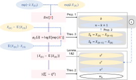
Figure 2: Roadmap of concentration proof. Variables related to left tail bound and right tail bound are specified by blue and yellow respectively. We upper bound the variables highlighted in pink in the order indicated by arrows between them. The upper bounds are functions of the blocks of variables pointed by solid arrows, with the corresponding theorem names on the arrow.

In the following, we apply the entropy method to order statistics and focus on our contributions in terms of the proof technique. We derive a technical result to bound the entropy in Proposition 1. The bound on entropy, along with another technical result on the spacing between consecutive order statistics allows us to derive an exponential Efron-Stein inequality (Theorem 3). Recall $X_{(1)}\geq\ldots\geq X_{(n)}$ are the order statistics of $X_{1},\ldots,X_{n}$. Define the spacing between order statistics of order $k$ and $k-1$ as

$$S_{k}:=X_{(k)}-X_{(k+1)};\quad S_{k-1}:=X_{(k-1)}-X_{(k)}.$$ (17)

We first show the upper bounds of entropy in terms of the spacing between order statistics in Proposition 1.

Proposition 1 (Entropy upper bounds).

Define $\phi(x):=\exp(x)-x-1$ and $\zeta(x):=\exp(x)\phi(-x)=1+(x-1)\exp(x)$. For all $\lambda\geq 0$, and for $k\in[1,n)\wedge\mathbb{N}^{\ast}$,

$$\operatorname{Ent}\left[\exp(\lambda X_{(k)})\right]\leq k\mathbb{E}\left[\exp(\lambda X_{(k+1)})\zeta\left(\lambda S_{k}\right)\right].$$ (18)

For $k\in(1,n]\wedge\mathbb{N}^{\ast}$,

$$\operatorname{Ent} \left[\exp(-\lambda X_{(k)})\right]\leq$$

$$(n-k+1)\mathbb{E}\left[\exp(-\lambda X_{(k)})\phi\left(-\lambda S_{k-1}\right)\right].$$ (19)

The upper bounds in Proposition 1 are expressed in terms of the corresponding order statistics and the spacing for consecutive order statistics. From Proposition 1, and by normalising entropy as shown in Eq. (16), we show the upper bound of the logarithmic moment generating function of $Z_{k}:=X_{(k)}-\mathbb{E}[X_{(k)}]$ and $Z_{k}^{\prime}:=\mathbb{E}[X_{(k)}]-X_{(k)}$.

Theorem 3 (Extended Exponential Efron-Stein inequality).

With the logarithmic moment generating function defined in Eq. 14, for $\lambda\geq 0$ and $k\in[1,n)\wedge\mathbb{N}^{\ast}$,

$$\psi_{Z_{k}}(\lambda)\leq\lambda\frac{k}{2}\mathbb{E}\left[S_{k}\left(\exp(\lambda S_{k})-1\right)\right].$$ (20)

For $k\in(1,n]\wedge\mathbb{N}^{\ast}$,

$$\psi_{Z_{k}^{\prime}}(\lambda)\leq\frac{\lambda^{2}(n-k+1)}{2}\mathbb{E}[S_{k-1}^{2}].$$ (21)

Observe that the upper bounds in Theorem 3 depend on the order statistics spacings $S_{k},S_{k-1}$ in expectation.

The non-decreasing hazard rate assumption (Assumption 1) allows us to upper bound the spacings in expectation. We show the upper bound of expected spacing in Proposition 2. Based on a similar proof technique of Proposition 2, we can further bound Theorem 3 and the results are shown in Lemma 1 and Lemma 2.

Proposition 2.

For any $k\in[1,n)\wedge\mathbb{N}^{\ast}$, the expectation of spacing $S_{k}$ defined in Eq. (17) can be bounded under Assumption 1, $\mathbb{E}[S_{k}]\leq\frac{1}{kL}.$

Remark 1 (Novelty of our proof techinique).

The results shown in this section may be of independent interest. (i) In Proposition 1, we show the upper bounds of both $\operatorname{Ent}\left[\exp(\lambda X_{(k)})\right]$ and $\operatorname{Ent}\left[\exp(-\lambda X_{(k)})\right]$ for all rank $k$ except extremes. This allows two-sided tail bounds to hold for all ranks except extremes. (ii) In Theorem 3, we show upper bounds of logarithmic moment generating function for both $X_{(k)}-\mathbb{E}[X_{(k)}]$ and $\mathbb{E}[X_{(k)}]-X_{(k)}$ w.r.t the order statistics spacing in expectation. The upper bound of $\mathbb{E}[X_{(k)}]-X_{(k)}$ is tighter (sub-Gaussian). (iii) We propose an upper bound for the expected order statistics spacing $S_{k}=X_{(k)}-X_{(k+1)}$ in Proposition 2.

4 Quantile Bandits Policy: Q-SAR

We consider the setting of multi-armed bandits with a finite number of arms $K$. For each arm $i\in\mathcal{K}=\{1,...,K\}$, the rewards are sampled from an unknown stationary reward distribution $F_{i}$. We assume arms are independent. The environment $\nu$ consists of the set of all reward distributions $F_{i}$, i.e. $\nu:=\{F_{i}:i\in\mathcal{K}\}$. The agent makes a sequence of decisions based on a policy $\pi$ for $N$ rounds, where each round is denoted by $t\in\{1,\dots,N\}$. We denote the arm chosen at round $t$ as $A_{t}$, and $T_{i}(t)$ as the number of times for arm $i$ was chosen at the end of round $t$, i.e. $T_{i}(t):=\sum_{s=1}^{t}\mathbb{I}\{A_{s}=i\}.$ At round $t$, the agent observes reward $X^{A_{t}}_{T_{A_{t}}(t)}$ sampled from $F_{A_{t}}$.

The quality of an arm is determined by the $\tau$-quantile of its reward distribution. Arms with higher $\tau$-quantile values are better. We order the arms according to optimality as $o_{1},\dots,o_{K}$ s.t. $Q^{\tau}_{o_{1}}\geq\dots\geq Q^{\tau}_{o_{K}}$. The optimal arm set of size $m$ is $\mathcal{S}_{m}^{\ast}=\{o_{1},\dots,o_{m}\}$. Without loss of generality, we assume $\mathcal{S}_{m}^{\ast}$ is unique. Following Audibert et al. (2010); Bubeck et al. (2013), we formulate our objective by the probability of error.

Definition 2 (Probability of error/misidentification).

We denote $\mathcal{S}_{m}^{N}\subset\mathcal{K}$ as the set of $m$ arms returned by the policy at the end of the exploration phase. Define the probability of error as

$$e_{N}:=\mathbb{P}\left(\mathcal{S}_{m}^{N}\neq\mathcal{S}_{m}^{\ast}\right).$$ (22)

The goal is, with a fixed budget of $N$ rounds, to design a policy which returns a set of arms of size $m\geq 1$ so that probability of error $e_{N}$ is minimised.

Algorithm 1 Q-SAR

  Let the active set $\mathcal{A}_{1}=\{1,...,K\}$, the accepted set $\mathcal{M}_{1}=\emptyset$, the number of arms left to find $l_{1}=m$,

  $\overline{\log}(K)=\frac{1}{2}+\sum_{i=2}^{K}\frac{1}{i},n_{0}=0$, and for $p\in\{1,...,K-1\},$ $n_{p}=\left\lceil\frac{1}{\overline{\log}(K)}\frac{N-K}{K+1-p}\right\rceil.$

  for each phase $p=1,2,...,K-1$ do

     (1) For each $i\in\mathcal{A}_{p}$, sample arm $i$ for $n_{p}-n_{p-1}$ times.

     (2) For each $i\in\mathcal{A}_{p}$, sort the empirical quantile of arm $i$ in a non-increasing order, denote the sorted arms as $a_{best},a_{2},...,a_{l_{p}},a_{l_{p}+1},...,a_{worst}$ (with ties broken arbitrarily).

     (3) Calculate $\widehat{\Delta}_{best}=\hat{Q}^{\tau}_{a_{best},n_{p}}-\hat{Q}^{\tau}_{a_{l_{p}+1},n_{p}}$, $\widehat{\Delta}_{worst}=\hat{Q}^{\tau}_{a_{l_{p}},n_{p}}-\hat{Q}^{\tau}_{a_{worst},n_{p}}$.

     if $\widehat{\Delta}_{best}>\widehat{\Delta}_{worst}$ then

        $\mathcal{A}_{p+1}=\mathcal{A}_{p}\backslash\{a_{best}\}$, $\mathcal{M}_{p+1}=\mathcal{M}_{p}\cup\{a_{best}\}$,

        $l_{p+1}=l_{p}-1$.

     else

        $\mathcal{A}_{p+1}=\mathcal{A}_{p}\backslash\{a_{worst}\}$, $\mathcal{M}_{p+1}=\mathcal{M}_{p},$

        $l_{p+1}=l_{p}$.

     end if

  end for

  Return the $m$ arms $\mathcal{S}_{m}^{N}=\mathcal{A}_{K}\cup\mathcal{M}_{K}$.

We propose a Quantile-based Successive Accepts and Rejects (Q-SAR) algorithm (Algorithm 1), which adapts the Successive Accepts and Rejects (SAR) algorithm (Bubeck et al., 2013). We divide the budget $N$ into $K-1$ phases. The number of samples drawn for each arm in each phase remains the same as in the Bubeck et al. (2013). At each phase $p\in\{1,2,\dots,K-1\}$, we maintain two sets (refer to Figure 3): i) the active set $\mathcal{A}_{p}$, which contains all arms that are actively drawn in phase $p$; ii) the accepted set $\mathcal{M}_{p}$, which contains arms that have been accepted. In each phase $p$, an arm is removed from the active set, and it is either accepted or rejected. The accepted arm is added into the accepted set. At the end of phase $K-1$, only one arm remains in the active set. The last remaining arm together with and the accepted set (containing $m-1$ arms) form the returned recommendation $\mathcal{S}_{m}^{N}$.

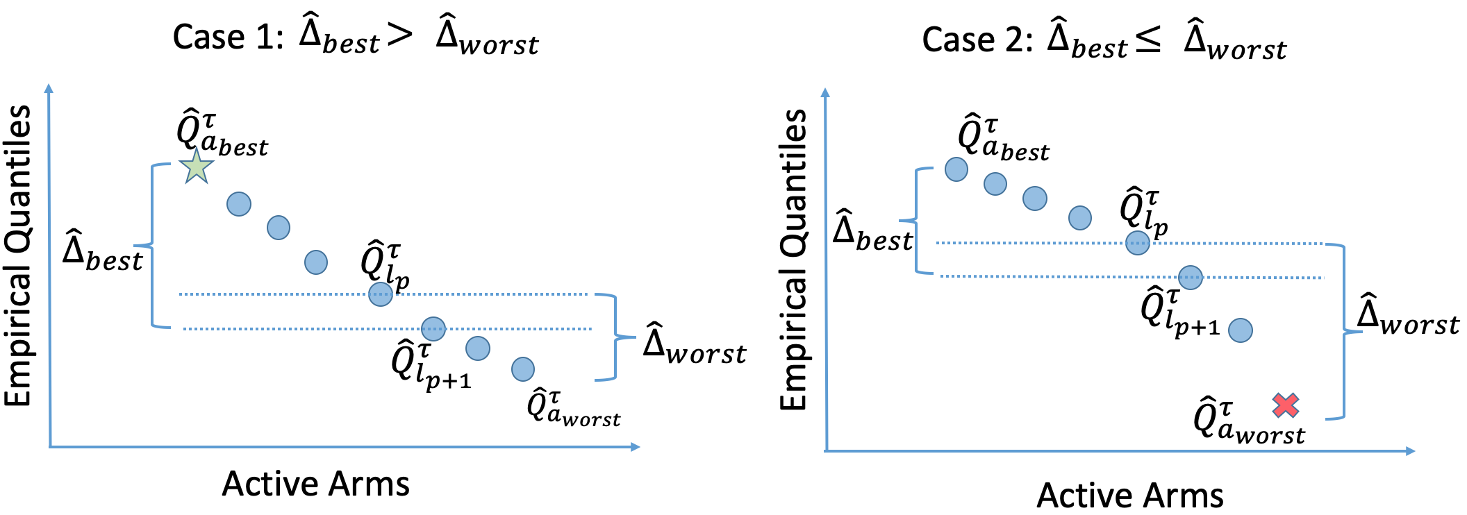
Figure 3: Phase $p$ of Q-SAR illustration. Star indicates accepted arm, cross indicates rejected arm.

We can consider the task of identifying $m$ best arms as grouping arms into the optimal set $\mathcal{S}_{m}^{\ast}$ and non-optimal set. Then intuitively it is easier to firstly group arms which are farther away from the boundary of the two groups, since the estimation error is less likely to influence the grouping (Refer to Figure 3). Q-SAR follows this intuition and determines to accept or reject the arm which is the farthest (based on estimates) from the boundary in each phase.

We introduce a simplified version of the SAR algorithm. Instead of considering all empirical gaps as SAR algorithm (Bubeck et al., 2013) proposed, Q-SAR decides whether to accept or reject an arm by only comparing two empirical gaps: $\widehat{\Delta}_{best}$ and $\widehat{\Delta}_{worst}$ (defined in Algorithm 1 step (3)). This simplification also applies when using the mean as a summary statistic, and results in an equivalent algorithm to the original SAR in (Bubeck et al., 2013). If $\widehat{\Delta}_{best}>\widehat{\Delta}_{worst}$, the arm with maximum empirical quantile is accepted; otherwise, the arm with minimum empirical quantile is rejected.

When $m=1$, $\widehat{\Delta}_{worst}=\hat{Q}^{\tau}_{a_{best}}-\hat{Q}^{\tau}_{a_{worst}}$, and $\widehat{\Delta}_{best}=\hat{Q}^{\tau}_{a_{best}}-\hat{Q}^{\tau}_{a_{2}}$. For all phases, $\widehat{\Delta}_{worst}\geq\widehat{\Delta}_{best}$, thus Q-SAR will keep rejecting arms. In this case, Q-SAR is the same as Q-SR (Algorithm 2, shown in Appendix A).

4.1 Theoretical Analysis

Recall optimality of arms are denoted as $o_{1},\dots,o_{K}$ s.t. $Q^{\tau}_{o_{1}}\geq\dots\geq Q^{\tau}_{o_{K}}$. The optimal arm set of size $m$ is $\mathcal{S}_{m}^{\ast}=\{o_{1},\dots,o_{m}\}$. For each arm $i\in\mathcal{K}$, we define the gap $\Delta_{i}\geq 0$ by

$$\Delta_{i}:=\left\{\begin{array}[]{ll}Q^{\tau}_{i}-Q^{\tau}_{o_{m+1}}&\text{ if }i\in\mathcal{S}_{m}^{\ast};\\ Q^{\tau}_{o_{m}}-Q^{\tau}_{i}&\text{ if }i\notin\mathcal{S}_{m}^{\ast}.\end{array}\right.$$

We sort the gaps in a non-decreasing order and denote the $i^{th}$ gap as $\Delta_{(i)}$, i.e. $\Delta_{(1)}\leq\Delta_{(2)}\leq\dots\leq\Delta_{(K)}$. The gaps characterise how separate the arms are and reflect the hardness of the problem. The smaller the (minimum) gaps of the arms are, the harder the BAI task is. We define the problem complexity $H^{\tau}$ as

$$H^{\tau}=\max_{\{i,j\in\mathcal{K}\}}\frac{8j}{1-\tau}(\frac{4\alpha}{L_{i}^{2}\Delta_{(j)}^{2}}+\frac{\beta_{i}}{L_{i}^{2}\Delta_{(j)}}).$$ (23)

where $\alpha=\frac{4(1+\tau)}{1-\tau},\beta_{i}=\frac{4}{3}(2L_{i}+b_{i}(1-\tau)L_{i}^{2})$, with $L_{i}$ as the lower bound of hazard rate of arm $i$.

To bound the probability of error under Q-SAR policy, it is convenient to re-express Theorem 2 such that the deviation between the empirical and true quantile is given by $\epsilon$. Observe that for Q-SAR, we are interested in events of small probability, that is for large values of $\gamma$ in Theorem 2. In the corollary below, we focus on such events of small probability by considering $\gamma\geq 1$ (i.e. error less than $\frac{1}{e}\approx 0.37$), which allows a simpler expression.

Corollary 1 (Representation of Concentration inequalities for Quantiles).

For $\epsilon>0$, $v^{r},v^{l},c^{r},w_{n}$ stay the same as stated in Theorem 2. With $\gamma\geq 1$, Theorem 2 can be represented as

$$\mathbb{P}\left(\hat{Q}^{\tau}_{n}-Q^{\tau}\geq\epsilon\right)\leq\exp\left(-\frac{{\epsilon}^{2}}{2(v^{r}+(c^{r}+w_{n})\epsilon)}\right),$$

$$\mathbb{P}\left(Q^{\tau}-\hat{Q}^{\tau}_{n}\geq\epsilon\right)\leq\exp\left(-\frac{{\epsilon}^{2}}{2(v^{l}+w_{n}\epsilon)}\right).$$

Applying Corollary 1, we show an upper bound of the probability of error in Theorem 4. Note we assume the total budget is at least $\frac{4}{1-\tau}\overline{\log}(K)+K$, which guarantees that after the initial round each arm has enough samples (See Lemma 3 in Appendix for details). We also present an error bound without assuming the lower bound of the budget in Theorem 8, based on concentration results in Lemma 4.

Theorem 4 (Q-SAR Probability of Error Upper Bound).

For the problem of identifying $m$ best arms out of $K$ arms, with budget $N\geq\frac{4}{1-\tau}\overline{\log}(K)+K$, the probability of error (Definition 2) for Q-SAR satisfies

$$e_{N}\leq 2K^{2}\exp\left(-\frac{N-K}{\overline{\log}(K)H^{\tau}}\right),$$

where problem complexity $H^{\tau}$ is defined in Eq. (23).

Observe the error bound depends on the problem complexity and has rate $\mathcal{O}(K^{2}\exp{(\frac{-N+K}{\log K})})$ w.r.t the number of arms $K$ and budget $N$. The smaller $H^{\tau}$ is, the smaller the upper bound of error probability is. In the following, we show a sketch of the proof. The detailed proof is provided in Appendix C.

Sketch of Proof.    Define the event $\xi$,

$$\xi:= \{\forall i\in\{1,\ldots,K\},p\in\{1,\ldots,K-1\},$$

$$\left|\hat{Q}^{\tau}_{i,n_{p}}-Q^{\tau}_{i}\right|<\frac{1}{4}\Delta_{(K+1-p)}\},$$ (24)

where $n_{p}$ is the number of samples at phase $p$ for arm $i$. One can upper bound $\mathbb{P}(\bar{\xi})$, i.e. the probability that complementary event of $\xi$ happens, by the union bound and our concentration results (Corollary 1). Then it suffices to show Q-SAR does not make any error on event $\xi$, which implies (I) no arm from the optimal set is rejected and (II) no arm from non-optimal set is accepted.

To show Q-SAR does not make any error on event $\xi$, we prove by induction on $p\geq 1$. In phase $p$, there are $K+1-p$ arms inside of the active set $\mathcal{A}_{p}$, we sort the arms inside of $\mathcal{A}_{p}$ and denote them as $\ell_{1},\ell_{2},\dots,\ell_{K+1-p}$ such that $Q^{\tau}_{\ell_{1}}\geq Q^{\tau}_{\ell_{2}}\geq\dots\geq Q^{\tau}_{\ell_{K+1-p}}$. We assume there is no wrong decision made in all previous $p-1$ phases and prove by contradiction. We assume that one arm from non-optimal set is accepted, or one arm from the optimal set is rejected in phase $p$. These two assumptions give us

$$\Delta_{(K+1-p)}>\max\left\{Q^{\tau}_{\ell_{1}}-Q^{\tau}_{o_{m+1}},Q^{\tau}_{o_{m}}-Q^{\tau}_{\ell_{K+1-p}}\right\},$$

which contradicts with the fact that $\Delta_{(K+1-p)}\leq\max\{Q^{\tau}_{\ell_{1}}-Q^{\tau}_{o_{m+1}},Q^{\tau}_{o_{m}}-Q^{\tau}_{\ell_{K+1-p}}\}$, since there are only $p-1$ arms that have been accepted or rejected at phase $p$. This concludes the proof. ∎

Comparison to related work: There are two problems in the standard MAB, namely the regret minimisation problems (Auer et al., 2002) and the Best Arm Identification (BAI) problems (Audibert et al., 2010). The goal of regret minimisation problems in bandit setting (Auer et al., 2002) is to maximise the cumulative rewards, i.e. minimise the cumulative regret. Best arm identification has been studied for fixed budget (Audibert et al., 2010) and fixed confidence (Even-Dar et al., 2006) settings. The difference between the two settings is how the exploration phase is terminated (when the budget runs out or when the quality of recommendations is at a fixed confidence level). We focus on the fixed budget setting for this work. For a comprehensive review of bandits we refer to Lattimore & Szepesvári (2020).
Previous quantile related BAI work (Szörényi et al., 2015; David & Shimkin, 2016; Yu & Nikolova, 2013; Howard & Ramdas, 2019) mostly focused on another setting of BAI, the fixed confidence setting. Literature concerning quantile bandits with the fixed budget is scarce. The most related work is Tran-Thanh & Yu (2014), which studied functional bandits, with quantiles as one example. They proposed the quantile based batch elimination algorithm. Since their concentration inequality is based on Chebyshev’s inequality (and hence not exponential), the upper bound on the probability of error has a rate $\mathcal{O}(K^{2}/N)$, which is slower than ours. Torossian et al. (2019) considered the fixed budget setting but focused on quantile optimization on stochastic black-box functions, which is different from our setting. As far as we know, Q-SAR is the first policy designed to identify multiple arms with highest $\tau$-quantile values.
The upper bound of error probability of Q-SAR and SAR (Bubeck et al., 2013) have the same rate (in terms of the budget $N$ and number of arms $K$) up to constant factors. Our constant term is smaller when the minimum lower bound of hazard rate takes a larger value. Unlike the mean-based algorithm, $H^{\tau}$ depends on the quantile level $\tau$ as well. The smaller $\tau$ is, the smaller the $H^{\tau}$ is. This can be intuitively explained as needing more samples to estimate higher level quantiles for IHR distributions.

5 Experiments

In this section, we illustrate how the proposed Q-SAR algorithm works on a toy example (Section 5.1) and demonstrate the empirical performance on a vaccine simulation (Section 5.2).

5.1 Illustrative Example

We set up simulated environments by constructing three arms with absolute Gaussian distribution or exponential distribution. The summary statistics of reward distributions are shown in Table 2. We expand the size of environments by replicating arms. Details about the experimental setting are shown in Appendix A.

We design two environments (sets of reward distributions) to show how one can benefit from considering quantiles as summary statistics with our algorithm. The design of the two environments reflects the two motivations in Section 1. Let $K$ be the total number of arms and $m$ be the number of arms to recommend. For each environment, we choose $m=1$ (single best arm identification) and $m=5$. We evaluate the probability of errors defined in Eq. (2). As a comparison, we introduce a Quantile-based Successive Rejects (Q-SR) algorithm in Algorithm 2 (Appendix A.3), which is adapted from Successive Rejects algorithm (Audibert et al., 2010) and we modify it to recommend multiple arms.

	Mean	0.5-Quantile	0.8-Quantile
A	1.60	1.35	2.55
B	3.60	3.50	5.21
C	4.00	2.76	6.42
Opt Arm	C	B	C
Min Gap	0.40	0.74	1.21

Table 2: Summary Statistics of Reward Distributions

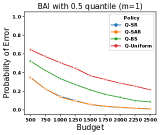
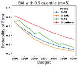
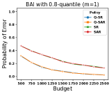
Figure 4: Illustrative examples. The first row shows the Environment I simulation where arms are evaluated by 0.5-quantiles. The second row shows the Environment II simulation where arms are evaluated by 0.8-quantiles (mean provides the same order of arms). We consider the task of recommending a single arm (left column) and recommending multiple arms ($m=5$, right column). The performance is evaluated in terms of the probability of error (with 5000 independent runs).

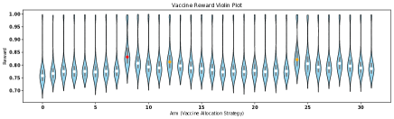
Figure 5: Vaccine Reward Violin Plot. The X-axis represents arms (vaccine allocation strategies), Y-axis represents rewards, which is the proportion of individuals that did not experience symptomatic infection. The circle in each violin represents the median, where the red one is the highest and the orange ones are the second and the third highest. The black line in each violin shows the range of 0.25-quantile to 0.75-quantile.

Environment I: We consider $K=20+m$ arms with 15 A arms, $m$ B (optimal) arms, and 5 C arms. The goal is to identify $m$ arms with largest $0.5$-quantile (i.e. median). We compare our algorithms with the quantile-based baseline algorithms: (i) Quantile uniform sampling (Q-Uniform), where each arm is sampled uniformly and we select the arm with the maximum 0.5-quantile; (ii) Quantile Batch Elimination (Q-BE) proposed in Tran-Thanh & Yu (2014) (iii) Quantile-based Successive Rejects (Q-SR).

Environment II: We consider $K=20+m$ arms with 15 A arms, 5 B arms, and $m$ C (optimal) arms. The goal is to identify $m$ arms with the maximum $0.8$-quantile. Both mean and 0.8-quantile provide the same order of arms, while 0.8-quantile can provide a larger gap compared with the mean. According to Theorem 4, the environment with a larger minimum gap has a smaller probability complexity and thus smaller upper bound of the probability of error (it holds for the mean-based algorithm (Bubeck et al., 2013) as well). We compare our algorithms with the baseline algorithms: (i) mean-based Successive Accepts and Rejects (SAR) (Bubeck et al., 2013). (ii) mean-based Successive Rejects (SR) (Audibert et al., 2010). (iii) Quantile-based Successive Rejects (Q-SR).

Results: We show the empirical probability of error as a function of budget in Figure 4. Q-SAR has the best performance under all settings. Q-SAR and Q-SR has the same performance for the single best arm identification ($m=1$) task in both environments, while Q-SAR outperforms Q-SR for multiple identifications ($m=5$). For Environment II, Q-SAR and Q-SR outperform SAR and SR since the gap between the optimal and suboptimal arms is bigger when evaluating arms by 0.8-quantiles than by means, and Q-SAR has a clear lower probability of error than Q-SR when the sample size is small.

5.2 Vaccine Simulation

We consider the problem of identifying optimal strategies for allocating an influenza vaccine. Following Libin et al. (2017), we format this problem as an instance of the BAI where each vaccine allocation strategy is an arm. Details of allocation strategies are available in the Appendix A.2. The reward of a strategy is defined as the proportion of individuals that did not experience symptomatic infection. We generate 1000 rewards for each strategy by simulating the epidemic for 180 days using FluTE  (with basic reproduction number $R_{0}=1.3$). The violin plot of reward samples is shown in Figure 5. The empirical reward distribution of arms are IHR, but with outliers close to 1 (which violate IHR). These outliers are due to the fact that the pathogen does not result in an epidemic in some simulation runs, which does not reflect the efficacy of the vaccine.

We use the median ($\tau=0.5$) as a robust summary statistic for each strategy. We apply our Q-SAR algorithm on two tasks. (1) the task of identifying $m=1$ best arm (index 8) with a fixed budget ranging from 500 to 2,500, and (2) the task of identifying $m=3$ best arms (index 8, 24 and 12) with a fixed budget ranging from 1,000 to 4,000. The performance for the BAI task is shown in Figure 6. We compare our algorithm other quantile-based algorithms only, since $0.5-$quantile and means results in different optimal arms. The empirical evidence shows Q-SAR is the best for multiple best arms identification (when $m=3$) and is robust to outliers. We leave the theoretical analysis for the outlier robustness of our approach as future work.

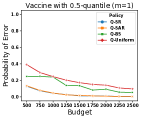
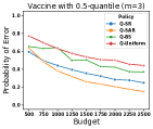
Figure 6: Vaccine BAI Experiments (with 5000 independent runs).

6 Conclusion and Discussion

Building on Boucheron & Thomas (2012), we prove a new concentration inequality of order statistics w.r.t its expectation, with which we prove a new concentration inequality for quantile estimation w.r.t. the population quantile. The new concentration inequalities are two-sided, and work for all distributions with non-decreasing hazard rate (IHR). Our assumption of positive (and unbounded) rewards results in asymmetric left and right tail bounds. The concentration inequalities for both order statistics and quantiles have convergence rate $\mathcal{O}(\sqrt{\frac{1}{n}})$. A larger value of $L$, the lower bound of the hazard rate, results in faster convergence. The proposed inequalities may be of independent interest.

In this paper, we consider the $m$ best arms identification problem with fixed budget. Motivated by risk-averse decision-making, the optimal arm set is determined by the $\tau$-quantiles of reward distributions instead of the mean. The quantile level $\tau$ provides an additional level of flexibility for modelling, depending on the risk preference. We proposed the quantile-based successive accepts and rejects (Q-SAR), the first quantile based bandit algorithm for the fixed budget setting. We apply our concentration inequality to prove an upper bound on error probability, which is characterised by the problem complexity. Empirical results show Q-SAR outperforms baseline algorithms for identifying multiple arms. One extension of this work is to allow different sample sizes in Q-SAR, that takes different quantile levels or lower bounds of hazard rate into consideration. Another future work is to derive the matching lower bound of error probability. We hope that this work opens the door towards new bandit approaches for other summary statistics.

Acknowledgements

The authors would like to thank Sébastien Bubeck for constructive suggestions about valid assumptions, Dawei Chen for generating the vaccine data, and Russell Tsuchida and Michael Yang for helpful comments.

Supplementary Materials for Quantile Bandits for Best Arms Identification

We show experiment details in Section A, the detailed proofs for both concentration inequalities (Section B) bandit task (Section C), and discussion in Section D.

Appendix A Experiments Details

In this section, we illustrate experiment details, including simulation details (Section A.1), vaccine allocation strategy description (Section A.2), Q-SR algorithm (Section A.3).

A.1 Illustrative Example

We provide more details about the environments setting in Section 5. We consider two distributions which satisfy our assumptions: absolute Gaussian distribution (Definition 3), and exponential distribution (Definition 4).

Definition 3 (Absolute Gaussian Distribution).

Given a Gaussian random variable $X$ with mean $\mu$ and variance $\sigma^{2}$, the random variable $Y=|X|$ has a absolute Gaussian distribution with p.d.f and c.d.f. shown as,

$$f_{AbsGau}(\mu,\sigma^{2})=\frac{1}{\sigma\sqrt{2\pi}}e^{-\frac{(x-\mu)^{2}}{2\sigma^{2}}}+\frac{1}{\sigma\sqrt{2\pi}}e^{-\frac{(x+\mu)^{2}}{2\sigma^{2}}},$$ (25)

$$F_{AbsGau}(\mu,\sigma^{2})=\frac{1}{2}\left[\operatorname{erf}\left(\frac{x+\mu}{\sigma\sqrt{2}}\right)+\operatorname{erf}\left(\frac{x-\mu}{\sigma\sqrt{2}}\right)\right].$$ (26)

where the error function $\text{erf}\left(x\right)=\frac{1}{\sqrt{\pi}}\int_{-x}^{x}e^{-t^{2}}dt$. We denote the absolute Gaussian distribution random variable with mean $\mu$ and variance $\sigma^{2}$ as $|\mathcal{N}(\mu,\sigma^{2})|$. When $\mu=0$, the lower bound of hazard rate $L=\frac{1}{\sigma\sqrt{2\pi}}$.

Definition 4 (Exponential Distribution).

With $\theta>0$, the p.d.f and c.d.f of exponential distribution are defined as

$$f_{Exp}\left(x,\theta\right) =\theta e^{-\theta x},$$ (27)

$$F_{Exp}\left(x,\theta\right) =1-e^{-\theta x},$$ (28)

We denote the exponential distribution with $\theta$ as $Exp(\theta)$. The hazard rate for exponential distribution is a constant and equal to $\theta$, i.e. $h(x)=\theta$.

We design our experimental environments based on three configurations of reward distributions: A) $|\mathcal{N}(0,2)|$ B) $|\mathcal{N}(3.5,2)|$ C) Exp(1/4). The histogram of these three arms is shown below.

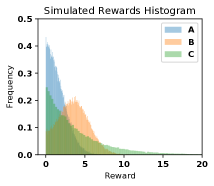
Figure 7: Simulated Arm Rewards Histogram.

A.2 Vaccine Allocation Strategy

We provide more details about the vaccine allocation strategy in this section. We allocate 100 vaccine doses (5$\%$ of the population) to 5 age groups (0-4 years, 5-18 years, 19-29 years, 30-64 years and $>$65 years). We consider all combinations of groups (resulting in $K=32$ arms), and denote the allocation scheme as a Boolean 5-tuple, with each position corresponds to the respective age group (1 represents allocation; 0 otherwise). We use the median ($\tau=0.5$) as a robust summary statistic for each strategy. For the task of identifying the best subset of ages ($m=1$) Q-SAR finds that the optimal arm is $(0,1,0,0,0)$, i.e. only allocation to 5-18 years old group. For identifying the $m=3$ best arms, the optimal arms are $(0,1,0,0,0),(1,1,0,0,0)$ and $(0,1,1,0,0)$, indicated as arms 8, 24, and 12 in Figure 5 respectively.

A.3 Q-SR

We extend the Successive Rejects algorithm (Audibert et al., 2010) to a quantile version and adapt it to recommend more than one arm.

Algorithm 2 Q-SR

  Denote the active set $\mathcal{A}_{1}=\{1,...,K\}$, $\widetilde{\log}(K)=\frac{m}{m+1}+\sum_{p=1}^{K-m}\frac{1}{K+1-p},n_{0}=0$, and for $k\in\{1,...,K-1\},$

  

$$n_{p}=\left\lceil\frac{1}{\widetilde{\log}(K)}\frac{N-K}{K+1-p}\right\rceil$$

  For each phase $p=1,2,...,K-m$:

  (1) For each $i\in\mathcal{A}_{p}$, select arm $i$ for $n_{p}-n_{p-1}$ rounds.

  (2) Let $\mathcal{A}_{p+1}=\mathcal{A}_{p}/\operatorname*{argmin}_{i\in\mathcal{A}_{p}}\hat{Q}^{\tau}_{i,n_{p}}$

  The recommended set is $\mathcal{A}_{K-m+1}$.

We provide justifications for the design choice of our proposed Q-SR algorithm shown in Algorithm 2. Although that both SR and SAR are analysed on reward distributions with support $[0,1]$, they can both be directly extended to subgaussian reward distributions (Audibert et al., 2010; Bubeck et al., 2013). We propose Quantile-based Successive Rejects (Q-SR), adapted from Successive Rejects (SR) algorithm (Audibert et al., 2010). To be able to recommend multiple arms, the total phase is designed to be $K-m$ instead of $K-1$, and the number of pulls for each round is modified to make sure all budgets are used. More precisely, one is pulled $n_{1}=\left\lceil\frac{1}{\widetilde{\log}(K)}\frac{N-K}{K}\right\rceil$ times, one is pulled $n_{2}=\left\lceil\frac{1}{\widetilde{\log}(K)}\frac{N-K}{K-1}\right\rceil$ times, $\dots$, $m+1$ is pulled $n_{K-m}=\left\lceil\frac{1}{\widetilde{\log}(K)}\frac{N-K}{K+1-(K-m)}\right\rceil$ times, then

$$n_{1}+\dots+(m+1)n_{K-m}\leq K+\frac{N-K}{\widetilde{\log}(K)}\left(\frac{m}{m+1}+\sum_{p=1}^{K-m}\frac{1}{K+1-p}\right)=N.$$ (29)

As shown in Section 4, when $m=1$, the Q-SAR algorithm can be reduced to the Q-SR algorithm. So the theoretical performance of the Q-SR algorithm is guaranteed. We leave the theoretical analysis of Q-SR for $m>1$ for the future work.

Appendix B Concentration Inequality Proof

This section shows the proofs of the concentration results shown in Section 2. In the following, we will walk through the key statement and show how we achieve our results in details. For the reader’s convenience, we restate our theorems in the main paper whenever needed. We first introduce the Modified logarithmic Sobolev inequality, which gives the upper bound of the entropy (Eq. (15)) of $\exp(\lambda W)$.

Theorem 5 (Modified logarithmic Sobolev inequality (Ledoux, 2001)).

Consider independent random variables $X_{1},\dots,X_{n}$, let a real-valued random variable $W=f\left(X_{1},\ldots,X_{n}\right)$, where $f:\mathbb{R}^{n}\rightarrow\mathbb{R}$ is measurable. Let $W_{i}=f_{i}\left(X_{1},\ldots,X_{i-1},X_{i+1},\ldots,X_{n}\right)$, where $f_{i}:\mathbb{R}^{n-1}\rightarrow\mathbb{R}$ is an arbitrary measurable function. Let $\phi(x)=\exp(x)-x-1$. Then for any $\lambda\in\mathbb{R}$,

$$\operatorname{Ent}\left[\exp(\lambda W)\right] =\lambda\mathbb{E}\left[W\exp(\lambda W)\right]-\mathbb{E}\left[\exp(\lambda W)\right]\log\mathbb{E}\left[\exp(\lambda W)\right]$$ (30)

$$\leq\sum_{i=1}^{n}\mathbb{E}\left[\exp(\lambda W)\phi\left(-\lambda\left(W-W_{i}\right)\right)\right]$$ (31)

Consider i.i.d random variables $X_{1},\dots,X_{n}$, and the corresponding order statistics $X_{(1)}\geq\dots\geq X_{(n)}$. Define the spacing between rank $k$ and $k+1$ order statistics as $S_{k}=X_{\left(k\right)}-X_{\left(k+1\right)}$. By taking $W$ as $k$ rank order statistics (or negative $k$ rank), and $W_{i}$ as nearest possible order statistics, i.e. $k\pm 1$ rank (or negative $k\pm 1$ rank), Theorem 5 provides the connection between the order statistics and the spacing between order statistics. The connection is shown in Proposition 1.

See 1

Proof.

We prove the upper bound based on Theorem 5. We first prove Eq. (18). We define $W,W_{i}$ with $f^{k}$, $f_{i}^{k}$ as following. Let $W$ be the rank $k$ order statistics of $X_{1},\dots,X_{n}$, i.e. $W=f^{k}(X_{1},\dots,X_{n})=X_{(k)}$; Let $W_{i}$ be the rank $k$ order statistics of $X_{1},\dots,X_{i-1},X_{i+1},\dots,X_{n}$ (i.e. with $X_{i}$ removed from $X_{1},\dots,X_{n}$), i.e. $f_{i}=X_{(k+1)}\mathbb{I}(X_{i}\geq X_{(k)})+X_{(k)}\mathbb{I}(X_{i}<X_{(k)})$. So $W_{i}=X_{(k+1)}$ when the removed element is bigger and equal to $X_{(k)}$, otherwise $W=X_{(k)}$. Then the upper bound of $\operatorname{Ent}\left[\exp(\lambda X_{(k)})\right]$ is

$$\operatorname{Ent}\left[\exp(\lambda X_{(k)})\right]$$

$$\leq \mathbb{E}\big{[}\sum_{i=1}^{n}\exp(\lambda X_{(k)})\phi\big{(}-\lambda(X_{(k)}-X_{(k+1)}\mathbb{I}(X_{i}\geq X_{(k)})-X_{(k)}\mathbb{I}(X_{i}<X_{(k)})\big{)}\big{]}$$ Theorem 5 (32)

$$= \mathbb{E}\big{[}\exp(\lambda X_{(k)})\phi\big{(}-\lambda(X_{(k)}-X_{(k+1)})\big{)}\sum_{i=1}^{n}\mathbb{I}(X_{i}\geq X_{(k)})\big{]}$$ (33)

$$= k\mathbb{E}\left[\exp(\lambda X_{(k)})\phi\left(-\lambda S_{k}\right)\right]$$ (34)

$$= k\mathbb{E}\left[\exp(\lambda X_{(k+1)})\exp(\lambda S_{k})\phi\left(-\lambda S_{k}\right)\right]$$ (35)

$$= k\mathbb{E}\left[\exp(\lambda X_{(k+1)})\zeta\left(\lambda S_{k}\right)\right] \zeta(x)=\exp(x)\phi(-x)$$ (36)

Similarly, for the proof of Eq. (1), We define $W,W_{i}$ with $\widetilde{f}^{k}$, $\widetilde{f}_{i}^{k-1}$. Let $W$ be the negative value of $k$ rank order statistics of $X_{1},\dots,X_{n}$, i.e. $W=\widetilde{f}^{k}(X_{1},\dots,X_{n})=-X_{(k)}$; Let $W_{i}$ be the negative value of ${k-1}$ rank order statistics of $X_{1},\dots,X_{i-1},X_{i+1},\dots,X_{n}$. Thus when $X_{i}\geq X_{(k-1)}$, $W_{i}=-X_{(k)}$, otherwise $W_{i}=-X_{(k-1)}$. Then by Theorem 5, we get $\operatorname{Ent}\left[\exp(-\lambda X_{(k)})\right]\leq(n-k+1)\mathbb{E}\left[\exp(-\lambda X_{(k)})\phi\left(-\lambda S_{k-1}\right)\right].$

∎

Compared with the proof in Boucheron & Thomas (2012), we do not choose a different initialisation of $W_{i}$ in terms of the two cases $k\leq n/2$ and $k>n/2$, which does not influence the concentration rates of empirical quantiles, and allows us to extend the proof to all ranks (excluding extremes). We derive upper bounds for both $\operatorname{Ent}\left[\exp(\lambda X_{(k)})\right]$ and $\operatorname{Ent}\left[\exp(-\lambda X_{(k)})\right]$, which allows us to derive two-sided concentration bounds instead of one-sided bound. Now we show the proof of Theorem 3.

See 3

Proof.

The proof of Eq. (20) is based on Proposition 1 and follows the same reasoning from (Boucheron & Thomas, 2012) Theorem 2.9. Note since Eq. (18) holds for $k\in[1,n)$, Eq. (20) can be proved for $k\in[1,n)$ (Boucheron & Thomas (2012) only proved for $k\in[1,n/2]$).

We now prove Eq. (21). Recall $\phi(x)=\exp(x)-x-1$. $\phi(x)$ is nonincreasing when $x\leq 0$ and nondecreasing otherwise. By Proposition 1 and Proposition 4 (which will be shown later), for $\lambda\geq 0$,

$$\operatorname{Ent}\left[\exp(-\lambda X_{(k)})\right]\leq (n-k+1)\mathbb{E}\left[\exp(-\lambda X_{(k)})\phi\left(-\lambda S_{k-1}\right)\right]$$ By Proposition 1 (37)

$$\leq (n-k+1)\mathbb{E}\left[\exp(-\lambda X_{(k)})\right]\mathbb{E}\left[\phi\left(-\lambda S_{k-1}\right)\right]$$ By Proposition 4 (38)

Multiplying both sides by $\exp(\lambda\mathbb{E}[X_{(k)}])$,

$$\operatorname{Ent}[\exp(\lambda Z_{k}^{\prime})]\leq(n-k+1)\mathbb{E}[\exp(\lambda Z_{k}^{\prime})]\mathbb{E}[\phi(-\lambda S_{k-1})].$$ (39)

With the fact $\phi(x)\leq\frac{1}{2}x^{2}$ when $x\leq 0$, and $-\lambda S_{k-1}\leq 0$, we have $\mathbb{E}[\phi(-\lambda S_{k-1})]\leq\frac{\lambda^{2}}{2}\mathbb{E}[S_{k-1}^{2}]$. We then obtain

$$\frac{\operatorname{Ent}\left[\exp(\lambda Z_{k}^{\prime})\right]}{\lambda^{2}\mathbb{E}\left[\exp(\lambda Z_{k}^{\prime})\right]}\leq\frac{n-k+1}{\lambda^{2}}\mathbb{E}[\phi(-\lambda S_{k-1})]\leq\frac{n-k+1}{2}\mathbb{E}[S_{k-1}^{2}].$$ (40)

We now solve this integral inequality. Integrating left side, with the fact that $\lim_{\lambda\rightarrow 0}\frac{1}{\lambda}\log\mathbb{E}\exp(\lambda Z_{k}^{\prime})=0$, for $\lambda\geq 0$, we have

$$\int_{0}^{\lambda}\frac{\operatorname{Ent}\left[\exp(tZ_{k}^{\prime})\right]}{t^{2}\mathbb{E}\left[\exp(tZ_{k}^{\prime})\right]}dt=\int_{0}^{\lambda}\frac{\mathbb{E}[tZ_{k}^{\prime}]-\log\mathbb{E}[\exp(tZ_{k}^{\prime})]}{t^{2}}dt=\frac{\log\mathbb{E}[\exp(tZ_{k}^{\prime})]}{t}|_{0}^{\lambda}= \frac{1}{\lambda}\log\mathbb{E}[\exp(\lambda Z_{k}^{\prime})].$$ (41)

Integrating right side, for $\lambda\geq 0$,

$$\int_{0}^{\lambda}\frac{n-k+1}{2}\mathbb{E}[S_{k-1}^{2}]dt=\frac{\lambda(n-k+1)}{2}\mathbb{E}[S_{k-1}^{2}].$$ (42)

Combining Eq. (40), (41) and (42), we get

$$\psi_{Z_{k}^{\prime}}(\lambda)=\log\mathbb{E}[\exp(\lambda Z_{k}^{\prime})]\leq\frac{\lambda^{2}(n-k+1)}{2}\mathbb{E}[S_{k-1}^{2}].$$ (43)

which concludes the proof.

∎

To further bound the order statistic spacings in expectation, we introduce the R-transform (Definition 5) and Rényi’s representation (Theorem 6). In the sequel, $f$ is a monotone function from $(a,b)$ to $(c,d)$, its generalised inverse $f^{\leftarrow}:(c,d)\rightarrow(a,b)$ is defined by $f^{\leftarrow}(y)=\inf\{x:a<x<b,f(x)\geq y\}$. Observe that the R-transform defined in Definition 5 is the quantile transformation with respect to the c.d.f of standard exponential distribution, i.e. $F^{\leftarrow}\left(F_{exp}\left(t\right)\right)$.

Definition 5 (R-transform).

The R-transform of a distribution F is defined as the non-decreasing function on $[0,\infty)$ by $R(t)=\inf\{x:F(x)\geq 1-\exp(-t)\}=F^{\leftarrow}(1-\exp(-t))$.

Theorem 6 (Rényi’s representation, Theorem 2.5 in (Boucheron & Thomas, 2012)).

Let $X_{\left(1\right)}\geq\ldots\geq X_{\left(n\right)}$ be the order statistics of samples from distribution F, $Y_{\left(1\right)}\geq Y_{\left(2\right)}\geq\ldots\geq Y_{\left(n\right)}$ be the order statistics of independent samples of the standard exponential distribution, then

$${\scriptstyle\left(Y_{\left(n\right)},\ldots,Y_{\left(k\right)},\ldots,Y_{\left(1\right)}\right)\stackrel{{\scriptstyle d}}{{=}}\left(\frac{E_{n}}{n},\ldots,\sum_{i=k}^{n}\frac{E_{i}}{i},\ldots,\sum_{i=1}^{n}\frac{E_{i}}{i}\right),}$$ (44)

where $E_{1},\ldots,E_{n}$ are independent and identically distributed (i.i.d.) standard exponential random variables, and

$$\left(X_{\left(n\right)},\ldots,X_{\left(1\right)}\right)\stackrel{{\scriptstyle d}}{{=}}\left(R\left(Y_{\left(n\right)}\right),\ldots,R\left(Y_{\left(1\right)}\right)\right),$$ (45)

where $R\left(\cdot\right)$ is the R-transform defined in Definition 5, equality in distribution is denoted by $\stackrel{{\scriptstyle d}}{{=}}$.

The Rényi’s representation shows the order statistics of an Exponential random variable are linear combinations of independent Exponentials, which can be extended to the representation for order statistics of a general continuous $F$ by quantile transformation using R-transform. The following proposition states the connection between the IHR and R-transform.

Proposition 3 (Proposition 2.7 (Boucheron & Thomas, 2012)).

Let F be an absolutely continuous distribution function with hazard rate h (assuming density exists), the derivative of R-transform is $R^{\prime}=1/h\left(R\right)$. Then if the hazard rate h is non-decreasing (Assumption 1), then for all $t>0$ and $x>0$, $R\left(t+x\right)-R(t)\leq x/h\left(R(t)\right).$

We now show Proposition 4 based on the Rényi’s representation (Theorem 6) and Harris’ inequality (Theorem 7). Proposition 4 allows us to upper bound the expectation of multiplication of two functions in terms of the multiplication of expectation of those two functions respectively. We will use this property to prove Theorem 3.

Theorem 7 (Harris’ inequality (Boucheron et al., 2013)).

Let $X_{1},\ldots,X_{n}$ be independent real-valued random variables and define the random vector $X=\left(X_{1},\ldots,X_{n}\right)$ taking values in $\mathbb{R}^{n}.$ If $f:\mathbb{R}^{n}\rightarrow\mathbb{R}$ is nonincreasing and $g:\mathbb{R}^{n}\rightarrow\mathbb{R}$ is nondecreasing then

$$\mathbb{E}[f(X)g(X)]\leq\mathbb{E}[f(X)]\mathbb{E}[g(X)]$$

Proposition 4 (Negative Association).

Let the order statistics spacing of rank $k-1$ as $S_{k-1}=X_{(k-1)}-X_{(k)}$. Then $X_{(k)}$ and $S_{k-1}$ are negatively associated: for any pair of non-increasing function $f_{1}$ and $f_{2}$,

$$\mathbb{E}\left[f_{1}(X_{(k)})f_{2}\left(S_{k-1}\right)\right]\leq\mathbb{E}\left[f_{1}(X_{(k)})\right]\mathbb{E}\left[f_{2}\left(S_{k-1}\right)\right].$$ (46)

Proof.

From Definition 5 and Theorem 6, let $Y_{(1)},\ldots,Y_{(n)}$ be the order statistics of an exponential sample. Let $E_{k-1}=$ $Y_{(k-1)}-Y_{(k)}$ be the ${(k-1)}^{\text{th }}$ spacing of the exponential sample. By Theorem 6, $E_{k-1}$ and $Y_{(k)}$ are independent.

$$\mathbb{E}\left[f_{1}\left(X_{(k)}\right)f_{2}\left(S_{k-1}\right)\right]= \mathbb{E}\left[f_{1}(R(Y_{(k)}))f_{2}\left(R(Y_{(k-1)})-R(Y_{(k)})\right)\right]$$ (47)

$$= \mathbb{E}\left[\mathbb{E}\left[f_{1}(R(Y_{(k)}))f_{2}\left(R(E_{k-1}+Y_{(k)})-R(Y_{(k)})\right)|Y_{(k)}\right]\right]$$ (48)

$$= \mathbb{E}\left[f_{1}(R(Y_{(k)}))\mathbb{E}\left[f_{2}\left(R(E_{k-1}+Y_{(k)})-R(Y_{(k)})\right)|Y_{(k)}\right]\right].$$ (49)

The function $f_{1}\circ R$ is non-increasing. Almost surely, the conditional distribution of $(k-1)E_{k-1}$ w.r.t $Y_{(k)}$ is the exponential distribution.

$$\mathbb{E}\left[f_{2}\left(R(E_{k-1}+Y_{(k)})-R(Y_{(k)})\right)|Y_{(k)}\right]=\int_{0}^{\infty}e^{-x}f_{2}(R(\frac{x}{k-1}+Y_{(k)})-R(Y_{(k)}))dx.$$ (50)

As $F$ is IHR, $R(\frac{x}{k-1}+y)-R(y)=\int_{0}^{x/(k-1)}R^{\prime}(y+z)dz$ is non-increasing w.r.t. $y$ (from Proposition 3 we know R is concave when F is IHR). Then $\mathbb{E}\left[f_{2}\left(R(E_{k-1}+Y_{(k)})-R(Y_{(k)})\right)|Y_{(k)}\right]$ is non-decreasing function of $Y_{(k)}$. By Harris’ inequality,

$$\mathbb{E}\left[f_{1}\left(X_{(k)}\right)f_{2}\left(S_{k-1}\right)\right]\leq \mathbb{E}\left[f_{1}(R(Y_{(k)}))\right]\mathbb{E}\left[\mathbb{E}\left[f_{2}\left(R(E_{k-1}+Y_{(k)})-R(Y_{(k)})\right)|Y_{(k)}\right]\right]$$ (51)

$$= \mathbb{E}\left[f_{1}(R(Y_{(k)}))\right]\mathbb{E}\left[f_{2}\left(R(E_{k-1}+Y_{(k)})-R(Y_{(k)})\right)\right]$$ (52)

$$= \mathbb{E}\left[f_{1}(X_{(k)})\right]\mathbb{E}\left[f_{2}(S_{k-1})\right].$$ (53)

∎

We prove Proposition 2 in the following by transform the spacing based on Rényi’s representation and the property described in Proposition 3.

See 2

Proof.

We show the upper bound the expectations of the $k^{th}$ spacing of order statistics, assuming the lower bound hazard rate is L. The following proof uses Proposition 3, which requires Assumption 1 hold.

$$\mathbb{E}[S_{k}] =\mathbb{E}[X_{(k)}-X_{(k+1)}]$$

$$=\mathbb{E}[R\left(Y_{\left(k+1\right)}+\frac{E_{k}}{k}\right)-R\left(Y_{\left(k+1\right)}\right)]$$ By Theorem 6 (54)

$$=\int_{Y}\int_{E}\left(R\left(y+\frac{z}{k}\right)-R\left(y\right)\right)f_{Y}\left(y\right)f_{E}\left(z\right)\mathrm{d}z\mathrm{d}y$$ (55)

$$\leq\int_{Y}\int_{E}\frac{z}{k\times h\left(R\left(y\right)\right)}f_{Y}\left(y\right)f_{E}\left(z\right)\mathrm{d}z\mathrm{d}y$$ By Proposition 3 (56)

$$\leq\int_{E}\frac{z}{kL}f_{E}\left(z\right)\mathrm{d}z=\frac{1}{kL} \text{$L$ is the lower bound of the hazard rate}.$$ (57)

∎

Using the same technique of shown in Proposition 2, we prove Lemma 1 and Lemma 2 by further bounding inequalities shown in Theorem 3.

See 1

Proof.

We first prove Eq. (6). From Theorem 6, we can represent the spacing as $S_{k}=X_{\left(k\right)}-X_{\left(k+1\right)}\stackrel{{\scriptstyle d}}{{=}}R\left(Y_{\left(k+1\right)+E_{k}/k}\right)-R\left(Y_{\left(k+1\right)}\right)$, where $E_{k}$ is standard exponentially distributed and independent of $Y_{\left(k+1\right)}$. The following proof uses Proposition 3, which requires Assumption 1 hold.

$$\psi_{Z_{k}}(\lambda)\leq \lambda\frac{k}{2}\mathbb{E}\left[S_{k}\left(\exp(\lambda S_{k})-1\right)\right]$$ By Theorem 3 (58)

$$\leq \lambda\frac{k}{2}\int_{E}\int_{Y}\frac{z}{h\left(R\left(y\right)\right)k}\left(\exp(\frac{\lambda z}{h\left(R\left(y\right)\right)k})-1\right)f_{Y}\left(y\right)f_{E}\left(z\right)\mathrm{d}y\mathrm{d}z$$ By Proposition 3 (59)

$$\leq \frac{k}{2}\int_{E}\frac{\lambda}{Lk}z\left(\exp(\frac{\lambda}{Lk}z)-1\right)f_{E}\left(z\right)\mathrm{d}z$$ (60)

$$= \frac{k}{2}\int_{0}^{\infty}\frac{\lambda}{Lk}z\left(\exp(\frac{\lambda}{Lk}z)-1\right)\exp(-z)\mathrm{d}z$$ (61)

$$\leq \frac{\lambda^{2}v^{r}}{2(1-c^{r}\lambda)}, \text{With }v^{r}=\frac{2}{kL^{2}},c^{r}=\frac{2}{kL}$$ (62)

The last step is because for $0\leq\mu\leq\frac{1}{2}$, $\int_{0}^{\infty}\mu z\left(\exp(\mu z)-1\right)\exp(-z)\mathrm{d}z=\frac{\mu^{2}\left(2-\mu\right)}{\left(1-\mu\right)^{2}}\leq\frac{2\mu^{2}}{1-2\mu}$. where we let $\mu=\frac{\lambda}{Lk}$.

From Eq. (6) to Eq. (7), we convert the bound of logarithmic moment generating function to the tail bound by using the Cramér-Chernoff method (Boucheron et al., 2013). Markov’s inequality implies, for $\lambda\geq 0$,

$$\mathbb{P}(Z_{k}\geq\gamma)\leq\exp(-\lambda\gamma)\mathbb{E}[\exp(\lambda Z_{k})].$$ (63)

To choose $\lambda$ to minimise the upper bound, one can introduce $\psi_{Z_{k}}^{*}(\gamma)=\sup_{\lambda\geq 0}\left(\lambda\gamma-\psi_{Z_{k}}(\lambda)\right)$. Then we get $\mathbb{P}(Z_{k}\geq\gamma)\leq\exp\left(-\psi_{Z_{k}}^{*}(\gamma)\right)$. Set $h_{1}(u):=1+u-\sqrt{1+2u}$ for $u>0$, we have

$$\psi^{\ast}_{Z_{k}}(t)=\operatorname{sup}_{\lambda\in(0,1/c^{r})}(\gamma\lambda-\frac{\lambda^{2}v^{r}}{2(1-c^{r}\lambda)})=\frac{v^{r}}{{(c^{r})}^{2}}h_{1}(\frac{c^{r}\gamma}{v^{r}})$$ (64)

Since $h_{1}$ is an increasing function from $(0,\infty)$ to $(0,\infty)$ with inverse function $h_{1}^{-1}(u)=u+\sqrt{2u}$ for $u>0$, we have $\psi^{\ast-1}(u)=\sqrt{2v^{r}u}+c^{r}u$. Eq. (7) is thus proved. ∎

See 2

Proof.

The proof is similar to the proof of Lemma 1. From Theorem 6, we can represent the spacing as $S_{k-1}=X_{\left(k-1\right)}-X_{\left(k\right)}\stackrel{{\scriptstyle d}}{{=}}R\left(Y_{\left(k\right)+E_{k-1}/(k-1)}\right)-R\left(Y_{\left(k\right)}\right)$, where $E_{k-1}$ is standard exponentially distributed and independent of $Y_{\left(k\right)}$. The following proof uses Proposition 3, which requires Assumption 1 hold.

$$\psi_{Z_{k}^{\prime}}(\lambda)\leq \frac{\lambda^{2}(n-k+1)}{2}\mathbb{E}[S_{k-1}^{2}]$$ By Theorem 3 (65)

$$\leq \frac{\lambda^{2}(n-k+1)}{2}\int_{Y}\int_{E}\left(\frac{z}{(k-1)\times h\left(R\left(y\right)\right)}\right)^{2}f_{Y}\left(y\right)f_{E}\left(z\right)\mathrm{d}z\mathrm{d}y$$ By Proposition 3 (66)

$$\leq \frac{\lambda^{2}(n-k+1)}{2}\int_{0}^{\infty}\left(\frac{z}{(k-1)L}\right)^{2}\exp(-z)\mathrm{d}z$$ (67)

$$\leq \frac{\lambda^{2}v^{l}}{2}. \text{With }v^{l}=\frac{2(n-k+1)}{(k-1)^{2}L^{2}}$$ (68)

Eq. (8) is proved. Follow the Cramér-Chernoff method described above, we can prove Eq. (9). ∎

The concentration results for order statistics can be of independent interest. For example, one can take this result and derive the concentration for sum of order statistics by applying Hoeffding’s inequality (Hoeffding, 1994) or Bernstein’s inequality (Bernstein, 1924). Kandasamy et al. (2018) took the results from Boucheron & Thomas (2012) and showed such results, but limited for right tail result for exponential random variables of rank 1 order statistics (i.e. maximum).

Now we convert the concentration results of order statistics to the quantiles, based on the results from Lemma 1 and 2, and the Theorem 1 , which shows connection between expected order statistics and quantiles.

See 2

Proof.

Denote the confidence interval for the right tail bound of order statistics as $d^{r}_{k,\gamma}=\sqrt{2v^{r}\gamma}+c^{r}\gamma$. From Lemma 1, we have $\mathbb{P}\left(X_{(k)}-\mathbb{E}[X_{(k)}]\geq d^{r}_{k,\gamma}\right)\leq\exp(-\gamma)$. With $k=\lfloor n(1-\tau)\rfloor$, we have $\hat{Q}^{\tau}_{n}=X_{(k)}$ and from Theorem 1, we have $\mathbb{E}[X_{(k)}]\leq Q^{\tau}+w_{n}$. With probability at least $1-\exp(-\gamma)$, the following event holds

$$X_{(k)}-\mathbb{E}[X_{(k)}]<d^{r}_{k,\gamma}\Rightarrow X_{(k)}<\mathbb{E}[X_{(k)}]+d^{r}_{k,\gamma}\leq Q^{\tau}+w_{n}+d^{r}_{k,\gamma}\Rightarrow\hat{Q}^{\tau}_{n}-Q^{\tau}<w_{n}+d^{r}_{k,\gamma},$$ (69)

from which we have $\mathbb{P}(\hat{Q}^{\tau}_{n}-Q^{\tau}\geq w_{n}+d^{r}_{k,\gamma})\leq\exp(-\gamma)$.

Denote the confidence interval for the right tail bound of order statistics as $d^{l}_{k,\gamma}=\sqrt{2v^{l}\gamma}$. From Lemma 2, we have $\mathbb{P}\left(\mathbb{E}[X_{(k)}]-X_{(k)}\geq d^{l}_{k,\gamma}\right)\leq\exp(-\gamma)$. With $k=\lfloor n(1-\tau)\rfloor$, we have $\hat{Q}^{\tau}_{n}=X_{(k)}$ and from Theorem 1, we have $\mathbb{E}[X_{(k)}]\geq Q^{\tau}-w_{n}$. With probability at least $1-\exp(-\gamma)$, the following event holds

$$\mathbb{E}[X_{(k)}]-X_{(k)}<d^{l}_{k,\gamma}\Rightarrow-X_{(k)}<-\mathbb{E}[X_{(k)}]+d^{l}_{k,\gamma}\leq-(Q^{\tau}-w_{n})+d^{l}_{k,\gamma}\Rightarrow Q^{\tau}-\hat{Q}^{\tau}_{n}<w_{n}+d^{l}_{k,\gamma},$$ (70)

from which we have $\mathbb{P}(Q^{\tau}-\hat{Q}^{\tau}_{n}\geq w_{n}+d^{l}_{k,\gamma})\leq\exp(-\gamma)$. This concludes the proof. ∎

In ths following, we show the representations for the concentration results.

Corollary 2 (Representation of Concentration inequalities for Order Statistics).

For $\epsilon>0$, the concentration inequalities for order statistics in Lemma 1 and 2 can be represented as

$$\mathbb{P}\left(X_{(k)}-\mathbb{E}[X_{(k)}]\geq\epsilon\right)\leq\exp\left(-\frac{{\epsilon}^{2}}{2(v^{r}+c^{r}\epsilon)}\right),$$ (71)

$$\mathbb{P}\left(\mathbb{E}[X_{(k)}]-X_{(k)}\geq\epsilon\right)\leq\exp\left(-\frac{{\epsilon}^{2}}{2v^{l}}\right).$$ (72)

Proof.

Eq. (72) follows by setting $\epsilon=\sqrt{2v^{l}\gamma}$. We now show the case for Eq. (71). Recall from the proof of Lemma 1 Eq. (64), $h_{1}(u)=1+u-\sqrt{1+2u}$. Follow the elementary inequality

$$h_{1}(u)\geq\frac{u^{2}}{2(1+u)}\quad u>0.$$ (73)

Lemma 1 implies $\psi_{Z_{k}}^{*}(t)\geq\frac{t^{2}}{2(v+ct)}$, so the statement Eq. (71) follows from Chernoff’s inequality. ∎

Recall that for Q-SAR, we are interested in events of small probability, that is for large values of $\gamma$ in Theorem 2. In the corollary below, we focus on such events of small probability by considering $\gamma\geq 1$ (i.e. error less than $\frac{1}{e}\approx 0.37$), which allows a simpler expression.

See 1

Proof.

With $\gamma\geq 1$, we have $\gamma w_{n}\geq w_{n}$, then with probability at least $1-\exp(-\gamma)$, we have

$$\hat{Q}^{\tau}_{n}-Q^{\tau}\leq\sqrt{2v^{r}\gamma}+c^{r}\gamma+w_{n}\leq\sqrt{2v^{r}\gamma}+c^{r}\gamma+w_{n}\gamma.$$

That is, we have

$$\mathbb{P}\left(\hat{Q}^{\tau}_{n}-Q^{\tau}\geq\sqrt{2v^{r}\gamma}+(c^{r}+w_{n})\gamma\right)\leq\exp(-\gamma).$$ (74)

Similarly, one can prove the other side. Then the similar reasoning as shown in proof of Corollary 2 concludes the proof. ∎

Appendix C Bandits Proof

In this section, we provide the proof for the bandit theoritical result (Section C.2), with a re-expression of the concentration result (Section C.1).

C.1 Re-expression of Concentration Results

The proof of Q-SAR error bound uses the concentration results for quantiles. We first further derive the result shown in Corollary 1 to show direct dependency on the number of samples $n$. Recall the rank $k=\lfloor n(1-\tau)\rfloor$ with quantile level $\tau\in(0,1)$, which can be re-expressed as

$$\frac{k}{1-\tau} \leq n\leq\frac{k+1}{1-\tau}$$ (75)

$$n(1-\tau)-1 \leq k\leq n(1-\tau).$$ (76)

We show the representation of concentration depending on $n$ in the following.

Lemma 3.

For $\epsilon>0$, recall $n$ denotes the number of samples, $b$ is a constant depending on the density about $\tau$-quantile ($0<\tau<1$), $L$ is the lower bound of hazard rate. With $n\geq\frac{4}{1-\tau}$, Corollary 1 can be represented as

$$\mathbb{P}\left(\hat{Q}^{\tau}_{n}-Q^{\tau}\geq\epsilon\right)\leq\exp\left(-\frac{n(1-\tau)L^{2}{\epsilon}^{2}}{2(\frac{8}{3}+\frac{4}{3}(2L+b(1-\tau)L^{2})\epsilon)}\right),$$

$$\mathbb{P}\left(Q^{\tau}-\hat{Q}^{\tau}_{n}\geq\epsilon\right)\leq\exp\left(-\frac{n(1-\tau)L^{2}{\epsilon}^{2}}{2(\frac{4(1+\tau)}{1-\tau}+b(1-\tau)L^{2}\epsilon)}\right).$$

Combining the two bounds together, we have the two-sided bound shown in the following,

$$\mathbb{P}\left(|\hat{Q}^{\tau}_{n}-Q^{\tau}|\geq\epsilon\right)\leq 2\exp\left(-\frac{n(1-\tau)L^{2}{\epsilon}^{2}}{2(\alpha+\beta\epsilon)}\right),$$

where $\alpha=\frac{4(1+\tau)}{1-\tau},\beta=\frac{4}{3}(2L+b(1-\tau)L^{2})$.

Proof.

By assuming $n\geq\frac{4}{1-\tau}$, we have

$$n(1-\tau)-1 =n(1-(\tau+\frac{1}{n}))\geq\frac{3}{4}n(1-\tau).$$ (77)

$$n(1-\tau)-2 =n(1-(\tau+\frac{2}{n}))\geq\frac{1}{2}n(1-\tau).$$ (78)

Recall $v^{r}=\frac{2}{kL^{2}}$, $v^{l}=\frac{2(n-k+1)}{(k-1)^{2}L^{2}}$, $c^{r}=\frac{2}{kL},w_{n}=\frac{b}{n}$, we have

$$\mathbb{P}\left(\hat{Q}^{\tau}_{n}-Q^{\tau}\geq\epsilon\right) \leq\exp\left(-\frac{{\epsilon}^{2}}{2(v^{r}+(c^{r}+w_{n})\epsilon)}\right)$$ (79)

$$=\exp\left(-\frac{{\epsilon}^{2}}{2(\frac{2}{kL^{2}}+(\frac{2}{kL}+\frac{b}{n})\epsilon)}\right)$$ (80)

$$\leq\exp\left(-\frac{{\epsilon}^{2}}{2(\frac{2}{kL^{2}}+(\frac{2}{kL}+\frac{b(1-\tau)}{k})\epsilon)}\right) n\geq\frac{k}{1-\tau}$$ (81)

$$=\exp\left(-\frac{kL^{2}{\epsilon}^{2}}{2(2+(2L+b(1-\tau)L^{2})\epsilon)}\right)$$ (82)

$$\leq\exp\left(-\frac{\frac{3}{4}n(1-\tau)L^{2}{\epsilon}^{2}}{2(2+(2L+b(1-\tau)L^{2})\epsilon)}\right) k\geq\frac{3}{4}n(1-\tau)$$ (83)

$$=\exp\left(-\frac{n(1-\tau)L^{2}{\epsilon}^{2}}{2(\frac{8}{3}+\frac{4}{3}(2L+b(1-\tau)L^{2})\epsilon)}\right).$$ (84)

Similarly,

$$\mathbb{P}\left(Q^{\tau}-\hat{Q}^{\tau}_{n}\geq\epsilon\right) \leq\exp\left(-\frac{{\epsilon}^{2}}{2(v^{l}+w_{n}\epsilon)}\right)$$ (85)

$$=\exp\left(-\frac{{\epsilon}^{2}}{2(\frac{2(n-k+1)}{(k-1)^{2}L^{2}}+\frac{b}{n}\epsilon)}\right)$$ (86)

$$\leq\exp\left(-\frac{{\epsilon}^{2}}{2(\frac{(1+\tau)}{1/4n(1-\tau)^{2}L^{2}}+\frac{b}{n}\epsilon)}\right) k-1\geq\frac{n(1-\tau)}{2}$$ (87)

$$=\exp\left(-\frac{{1/4n(1-\tau)^{2}L^{2}\epsilon}^{2}}{2((1+\tau)+1/4b(1-\tau)^{2}L^{2}\epsilon)}\right)$$ (88)

$$=\exp\left(-\frac{{n(1-\tau)L^{2}\epsilon}^{2}}{2(\frac{4(1+\tau)}{1-\tau}+b(1-\tau)L^{2}\epsilon)}\right).$$ (89)

Then let $\alpha=\max\{\frac{8}{3},\frac{4(1+\tau)}{1-\tau}\}=\frac{4(1+\tau)}{1-\tau},\beta=\max\{\frac{4}{3}(2L+b(1-\tau)L^{2}),b(1-\tau)L^{2}\}=\frac{4}{3}(2L+b(1-\tau)L^{2}))$, we have

$$\mathbb{P}\left(|\hat{Q}^{\tau}_{n}-Q^{\tau}|\geq\epsilon\right) =\mathbb{P}\left(\hat{Q}^{\tau}_{n}-Q^{\tau}\geq\epsilon\right)+\mathbb{P}\left(Q^{\tau}-\hat{Q}^{\tau}_{n}\geq\epsilon\right)$$

$$\leq 2\exp\left(-\frac{n(1-\tau)L^{2}{\epsilon}^{2}}{2(\alpha+\beta\epsilon)}\right).$$

∎

Remark 2 (Lower bound of sample size).

In Lemma 3, we make an assumption about the lower bound of sample size, i.e. $n\geq\frac{4}{1-\tau}$. Note that along with the left inequality of Equation (75), the lower bound of sample size can be expressed as $n\geq\frac{\max\{k,4\}}{1-\tau}$. When $k\geq 4$, we have $n\geq\frac{k}{1-\tau}=\frac{\lfloor n(1-\tau)\rfloor}{1-\tau}$, which holds for all $n\geq 1$. This implies that instead of making an assumption about sample size $n$, we could equivalently make an assumption about the rank ($k\geq 4$) or the quantile level ($\tau\leq 1-\frac{4}{n}$ with $n\geq 4$).
Note the constant 4 in $n\geq\frac{4}{1-\tau}$ is chosen to have a simpler expression for the concentration bounds, one can choose any constant bigger than 2 (such that the term $n(1-\tau)-2$ is valid in Equation (78)).

We show a variant of Lemma 3 where we remove the lower bound assumption of the number of samples. The derived concentration bounds have a constant term, which does not influence the convergence rate in terms of $n$.

Lemma 4.

For $\epsilon>0$, recall $n$ denotes the number of samples, $b$ is a constant depending on the density about $\tau$-quantile ($0<\tau<1$), $L$ is the lower bound of hazard rate. Corollary 1 can be represented as

$$\mathbb{P}\left(\hat{Q}^{\tau}_{n}-Q^{\tau}\geq\epsilon\right)\leq\exp\left(-\frac{n(1-\tau)L^{2}{\epsilon}^{2}}{2(2+(2L+b(1-\tau)L^{2})\epsilon)}+\frac{L^{2}{\epsilon}^{2}}{2(2+(2L+b(1-\tau)L^{2})\epsilon)}\right),$$

$$\mathbb{P}\left(Q^{\tau}-\hat{Q}^{\tau}_{n}\geq\epsilon\right)\leq\exp\left(-\frac{n(1-\tau)L^{2}{\epsilon}^{2}}{2(\frac{2(2+\tau)}{1-\tau}+b(1-\tau)L^{2}\epsilon)}+\frac{L^{2}{\epsilon}^{2}}{2(\frac{1}{2}\frac{\tau}{1-\tau}+\frac{1}{4}b(1-\tau)L^{2}\epsilon)}\right).$$

Combining the two bounds together, we have the two-sided bound shown in the following,

$$\mathbb{P}\left(|\hat{Q}^{\tau}_{n}-Q^{\tau}|\geq\epsilon\right)\leq 2\exp\left(-\frac{n(1-\tau)L^{2}{\epsilon}^{2}}{2(\widetilde{\alpha}+\widetilde{\beta}\epsilon)}+\frac{L^{2}{\epsilon}^{2}}{2(\widetilde{\alpha}+\widetilde{\beta}\epsilon)}\right),$$

where $\widetilde{\alpha}=2\frac{\tau+2}{1-\tau},\widetilde{\beta}=2L+b(1-\tau)L^{2}$.

Proof.

From Eq. (82), we have

$$\mathbb{P}\left(\hat{Q}^{\tau}_{n}-Q^{\tau}\geq\epsilon\right) \leq\exp\left(-\frac{kL^{2}{\epsilon}^{2}}{2(2+(2L+b(1-\tau)L^{2})\epsilon)}\right)$$ (90)

$$\leq\exp\left(-\frac{(n(1-\tau)-1)L^{2}{\epsilon}^{2}}{2(2+(2L+b(1-\tau)L^{2})\epsilon)}\right) k\geq n(1-\tau)-1$$ (91)

$$=\exp\left(-\frac{(n(1-\tau))L^{2}{\epsilon}^{2}}{2(2+(2L+b(1-\tau)L^{2})\epsilon)}+\frac{L^{2}{\epsilon}^{2}}{2(2+(2L+b(1-\tau)L^{2})\epsilon)}\right).$$ (92)

From Eq. (86), we have

$$\mathbb{P}\left(Q^{\tau}-\hat{Q}^{\tau}_{n}\geq\epsilon\right) \leq\exp\left(-\frac{{\epsilon}^{2}}{2(\frac{2(n-k+1)}{(k-1)^{2}L^{2}}+\frac{b}{n}\epsilon)}\right)$$ (93)

$$\leq\exp\left(-\frac{L^{2}{\epsilon}^{2}}{2(\frac{2(n\tau+2)}{(n(1-\tau)-2)^{2}}+\frac{bL^{2}}{n}\epsilon)}\right) k-1\geq n(1-\tau)-2$$ (94)

$$\leq\exp\left(-\frac{L^{2}{\epsilon}^{2}}{2(\frac{2(n\tau+2)}{(n(1-\tau))(n(1-\tau)-4)}+\frac{bL^{2}}{n}\epsilon)}\right)$$ (95)

$$=\exp\left(-\frac{(n(1-\tau))(n(1-\tau)-4)L^{2}{\epsilon}^{2}}{2(2(n\tau+2)+n(1-\tau)^{2}bL^{2}\epsilon)}\right)$$ (96)

$$=\exp\left(-\frac{n(1-\tau)L^{2}{\epsilon}^{2}}{2(2\frac{\tau+2/n}{1-\tau}+(1-\tau)bL^{2}\epsilon)}+\frac{L^{2}{\epsilon}^{2}}{2(\frac{1}{2}\frac{(n\tau+2)}{n(1-\tau)}+\frac{1}{4}(1-\tau)bL^{2}\epsilon)}\right)$$ (97)

$$\leq\exp\left(-\frac{n(1-\tau)L^{2}{\epsilon}^{2}}{2(2\frac{\tau+2}{1-\tau}+b(1-\tau)L^{2}\epsilon)}+\frac{L^{2}{\epsilon}^{2}}{2(\frac{1}{2}\frac{\tau}{1-\tau}+\frac{1}{4}b(1-\tau)L^{2}\epsilon)}\right). n\geq 1\rightarrow 1/n\leq 1$$ (98)

Then let $\widetilde{\alpha}=2\max\left\{1,\frac{\tau+2}{1-\tau},\frac{1}{4}\frac{\tau}{1-\tau}\right\}=2\frac{\tau+2}{1-\tau}$, $\widetilde{\beta}=\max\{2L+b(1-\tau)L^{2},b(1-\tau)L^{2},\frac{1}{4}b(1-\tau)L^{2})\}=2L+b(1-\tau)L^{2}$. we have

$$\mathbb{P}\left(|\hat{Q}^{\tau}_{n}-Q^{\tau}|\geq\epsilon\right) =\mathbb{P}\left(\hat{Q}^{\tau}_{n}-Q^{\tau}\geq\epsilon\right)+\mathbb{P}\left(Q^{\tau}-\hat{Q}^{\tau}_{n}\geq\epsilon\right)\leq 2\exp\left(-\frac{n(1-\tau)L^{2}{\epsilon}^{2}}{2(\widetilde{\alpha}+\widetilde{\beta}\epsilon)}+\frac{L^{2}{\epsilon}^{2}}{2(\widetilde{\alpha}+\widetilde{\beta}\epsilon)}\right).$$

∎

Remark 3 (Constant term in concentration bound).

Note the constant term $\frac{L^{2}{\epsilon}^{2}}{2(\widetilde{\alpha}+\widetilde{\beta}\epsilon)}$ in Lemma 4 is due to the floor operator of the rank $k$, as explained in Eq. (75). This constant term is a bias term coming from estimating the quantile by a single order statistic and is unavoidable without additional assumptions.
By comparing Lemma 3 and Lemma 4 we observe that one needs to balance between the constant term, convergence rate, and assumptions to be made. For example, Lemma 3 reduces the constant term by assuming a lower bound on the sample size. On one hand, this assumption guarantees there is enough number of samples to have a more accurate estimation; on the other hand, compared with Lemma 4, Lemma 3 has a smaller convergence rate in terms of $n$ (larger parameters $\alpha,\beta$).

C.2 Q-SAR Error Bounds

In this section, we show the proof of Q-SAR error bounds, based on the concentration results we proposed. In Theorem 4, we show the error bound based on Lemma 3 under the assumption of lower bound of budget. In Theorem 8, we release the budget assumption, and show a variant of the error bound based on Lemma 4. The proof technique follows Bubeck et al. (2013).

See 4

Proof.

Recall we order the arms according to optimality as $o_{1},\dots,o_{K}$ s.t. $Q^{\tau}_{o_{1}}\geq\dots\geq Q^{\tau}_{o_{K}}$. The optimal arm set of size $m$ is $\mathcal{S}_{m}^{\ast}=\{o_{1},\dots,o_{m}\}$. In phase $p$, there are $K+1-p$ arms inside of the active set $\mathcal{A}_{p}$, we sort the arms inside of $\mathcal{A}_{p}$ and denote them as $\ell_{1},\ell_{2},\dots,\ell_{K+1-p}$ such that $Q^{\tau}_{\ell_{1}}\geq Q^{\tau}_{\ell_{2}}\geq\dots\geq Q^{\tau}_{\ell_{K+1-p}}$. If the algorithm does not make any error in the first $p-1$ phases (i.e. not reject an arm from optimal set and not accept an arm from non-optimal set), then we have

$$\{\ell_{1},\ell_{2},\ldots,\ell_{l_{p}}\}\subseteq\mathcal{S}_{m}^{\ast},\quad\{\ell_{l_{p}+1},\ldots,\ell_{K+1-p}\}\subseteq\mathcal{K}\backslash\mathcal{S}_{m}^{\ast}.$$ (99)

Additionally, we sort the arms in $\mathcal{A}_{p}$ according to the empirical quantiles at phase $p$ as $a_{best}(=a_{1}),a_{2},...,a_{l_{p}},a_{l_{p}+1},...,a_{worst}(=a_{K-p+1})$ such that $\hat{Q}^{\tau}_{a_{best},n_{p}}\geq\hat{Q}^{\tau}_{a_{2},n_{p}}\geq\dots\geq\hat{Q}^{\tau}_{a_{worst},n_{p}}$.

Consider an event $\xi$,

$$\xi=\{\forall i\in\{1,\ldots,K\},p\in\{1,\ldots,K-1\},\left|\hat{Q}^{\tau}_{i,n_{p}}-Q^{\tau}_{i}\right|<\frac{1}{4}\Delta_{(K+1-p)}\}.$$

Recall $\alpha=\frac{4(1+\tau)}{1-\tau}$, and we adapt $\beta$ to $\beta_{i}$ with $i$ indicating the index of arm, that is, $\beta_{i}=\frac{4}{3}(2L_{i}+b_{i}(1-\tau)L_{i}^{2})$. Recall the sample size for phase $p$ is $n_{p}=\lceil\frac{N-K}{\overline{\log}(K)(K+1-p)}\rceil$. Based on Lemma 3 and the union bound, we derive the upper bound of probability for the complementary event $\bar{\xi}$ as

$$\mathbb{P}(\bar{\xi}) \leq\sum_{i=1}^{K}\sum_{p=1}^{K-1}\mathbb{P}\left(\left|\hat{Q}^{\tau}_{i,n_{p}}-Q^{\tau}_{i}\right|\geq\frac{1}{4}\Delta_{(K+1-p)}\right)$$ union bound (100)

$$\leq\sum_{i=1}^{K}\sum_{p=1}^{K-1}2\exp\left(-\frac{n_{p}(1-\tau)L_{i}^{2}{(\frac{1}{4}\Delta_{(K+1-p)})}^{2}}{2(\alpha+\beta_{i}\frac{1}{4}\Delta_{(K+1-p)})}\right)$$ By Lemma 3 (101)

$$\leq\sum_{i=1}^{K}\sum_{p=1}^{K-1}2\exp\left(-\frac{N-K}{\overline{\log}(K)(K+1-p)}\frac{1}{\frac{8}{1-\tau}(\frac{4\alpha}{L_{i}^{2}\Delta_{(K+1-p)}^{2}}+\frac{\beta_{i}}{L_{i}^{2}\Delta_{(K+1-p)}})}\right)$$ (102)

$$\leq 2K^{2}\exp\left(-\frac{N-K}{\overline{\log}(K)H^{\tau}}\right).$$ (103)

where $H^{\tau}=\max_{\{i,j\in\mathcal{K}\}}\frac{8j}{1-\tau}(\frac{4\alpha}{L_{i}^{2}\Delta_{(j)}^{2}}+\frac{\beta_{i}}{L_{i}^{2}\Delta_{(j)}})$.

Note that we have assumed the number of samples of each arm is at least $\frac{4}{1-\tau}$ in Lemma 3. That is, $Kn_{1}=K\lceil\frac{N-K}{\overline{\log}(K)K}\rceil\geq\frac{4}{1-\tau}$, which gives $N\geq\frac{4}{1-\tau}\overline{\log}(K)+K$. This means, the bound derived above holds when we have budget $N$ no less than $\frac{4}{1-\tau}\overline{\log}(K)+K$.

We show that on event $\xi$, Q-SAR algorithm does not make any error by induction on phases. Assume that the algorithm does not make any error on the first $p-1$ phases, i.e. does not reject an arm from optimal set and not accept an arm from non-optimal set. Then in the following, we show the algorithm does not make an error on the $p^{th}$ phase. We discuss in terms of two cases:

Case 1: If an arm $\ell_{j}$ is accepted, then $\ell_{j}\in\mathcal{S}_{m}^{\ast}$.
We prove by contradiction. Assume arm $\ell_{j}$ is accepted in phase $p$, but $\ell_{j}\notin\mathcal{S}_{m}^{\ast}$, i.e. $Q^{\tau}_{\ell_{j}}\leq Q^{\tau}_{\ell_{l_{p}+1}}\leq Q^{\tau}_{o_{m+1}}$. According to Algorithm 1, arm $\ell_{j}$ is accepted only if its empirical quantile is the maximum among all active arms in phase $p$, thus $\hat{Q}^{\tau}_{\ell_{j},n_{p}}\geq\hat{Q}^{\tau}_{\ell_{1},n_{p}}$. On event $\xi$, we have

$$Q^{\tau}_{\ell_{j}}+\frac{1}{4}\Delta_{(K+1-p)}>\hat{Q}^{\tau}_{\ell_{j},n_{p}}\geq\hat{Q}^{\tau}_{\ell_{1},n_{p}}>Q^{\tau}_{\ell_{1}}-\frac{1}{4}\Delta_{(K+1-p)}$$ (104)

$$\Rightarrow\Delta_{(K+1-p)}>\frac{1}{2}\Delta_{(K+1-p)}>Q^{\tau}_{\ell_{1}}-Q^{\tau}_{\ell_{j}}\geq Q^{\tau}_{\ell_{1}}-Q^{\tau}_{o_{m+1}}.$$ (105)

Another requirement to accept $\ell_{j}$ is $\widehat{\Delta}_{best}>\widehat{\Delta}_{worst}$, that is,

$$\hat{Q}^{\tau}_{\ell_{j},n_{p}}-\hat{Q}^{\tau}_{a_{l_{p}+1},n_{p}}>\hat{Q}^{\tau}_{a_{l_{p}},n_{p}}-\hat{Q}^{\tau}_{a_{K+1-p},n_{p}}.$$ (106)

In the following, we will connect Eq. (106) with the corresponding population quantiles on event $\xi$. We first connect $\hat{Q}^{\tau}_{a_{K+1-p},n_{p}}$ and $Q^{\tau}_{\ell_{K+1-p}}$. Since $\hat{Q}^{\tau}_{a_{K+1-p},n_{p}}$ is the minimum empirical quantile at phase $p$,

$$\hat{Q}^{\tau}_{a_{K+1-p},n_{p}}\leq\hat{Q}^{\tau}_{\ell_{K+1-p},n_{p}}<Q^{\tau}_{\ell_{K+1-p}}+\frac{1}{4}\Delta_{(K+1-p)}.$$ (107)

We then connect $\hat{Q}^{\tau}_{a_{l_{p}+1},n_{p}},\hat{Q}^{\tau}_{a_{l_{p}},n_{p}}$ to $Q^{\tau}_{o_{m}}$. On event $\xi$, for all $i\leq l_{p}$,

$$\hat{Q}^{\tau}_{\ell_{i},n_{p}}>Q^{\tau}_{\ell_{i}}-\frac{1}{4}\Delta_{(K+1-p)}\geq Q^{\tau}_{\ell_{l_{p}}}-\frac{1}{4}\Delta_{(K+1-p)}\geq Q^{\tau}_{o_{m}}-\frac{1}{4}\Delta_{(K+1-p)},$$ (108)

which means there are $l_{p}$ arms in active set, i.e. $\{\ell_{1},\ell_{2},\dots,\ell_{l_{p}}\}$, having empirical quantiles bigger or equal than $Q^{\tau}_{o_{m}}-\frac{1}{4}\Delta_{(K+1-p)}$. Additionally, although $j>l_{p}$, $\ell_{j}$ has the maximum empirical quantile, which is bigger than $Q^{\tau}_{o_{m}}-\frac{1}{4}\Delta_{(K+1-p)}$ as well. So in total there are $l_{p}+1$ arms having empirical quantiles bigger or equal to $Q^{\tau}_{o_{m}}-\frac{1}{4}\Delta_{(K+1-p)}$, i.e.

$$\hat{Q}^{\tau}_{a_{l_{p}},n_{p}}\geq\hat{Q}^{\tau}_{a_{l_{p}+1},n_{p}}\geq Q^{\tau}_{o_{m}}-\frac{1}{4}\Delta_{(K+1-p)}.$$ (109)

Combine Eq. (106)(107)(109) together, we have

$$(Q^{\tau}_{\ell_{j}}+\frac{1}{4}\Delta_{(K+1-p)})-(Q^{\tau}_{o_{m}}-\frac{1}{4}\Delta_{(K+1-p)})>(Q^{\tau}_{o_{m}}-\frac{1}{4}\Delta_{(K+1-p)})-(Q^{\tau}_{\ell_{K+1-p}}+\frac{1}{4}\Delta_{(K+1-p)})$$ (110)

$$\Rightarrow\Delta_{(K+1-p)}>2Q^{\tau}_{o_{m}}-(Q^{\tau}_{\ell_{j}}+Q^{\tau}_{\ell_{K+1-p}})>Q^{\tau}_{o_{m}}-Q^{\tau}_{\ell_{K+1-p}}.$$ (111)

From Eq. (105)(111), we have $\Delta_{(K+1-p)}>\max\{Q^{\tau}_{\ell_{1}}-Q^{\tau}_{o_{m+1}},Q^{\tau}_{o_{m}}-Q^{\tau}_{\ell_{K+1-p}}\},$ which contradicts the fact that $\Delta_{(K+1-p)}\leq\max\{Q^{\tau}_{\ell_{1}}-Q^{\tau}_{o_{m+1}},Q^{\tau}_{o_{m}}-Q^{\tau}_{\ell_{K+1-p}}\}$, since at phase $p$, there are only $p-1$ arms have been accepted or rejected. So we have if an arm $\ell_{j}$ is accepted, then $\ell_{j}\in\mathcal{S}_{m}^{\ast}$, which finishes the proof of Case 1.

Case 2: If an arm $\ell_{j}$ is rejected, the $\ell_{j}\notin\mathcal{S}_{m}^{\ast}$.

The proof of Case 2 is similar to the proof of Case 1. We prove by contradiction. Assume arm $\ell_{j}$ is rejected in phase $p$, but $\ell_{j}\in\mathcal{S}_{m}^{\ast}$, i.e. $Q^{\tau}_{\ell_{j}}\geq Q^{\tau}_{\ell_{l_{p}}}\geq Q^{\tau}_{o_{m}}$. According to Algorithm 1, arm $\ell_{j}$ is rejected only if its empirical quantile is the minimum among all active arms in phase $p$, thus $\hat{Q}^{\tau}_{\ell_{j},n_{p}}\leq\hat{Q}^{\tau}_{\ell_{K+1-p},n_{p}}$. On event $\xi$, we have

$$Q^{\tau}_{\ell_{j}}-\frac{1}{4}\Delta_{(K+1-p)}<\hat{Q}^{\tau}_{\ell_{j},n_{p}}\leq\hat{Q}^{\tau}_{\ell_{K+1-p},n_{p}}<Q^{\tau}_{\ell_{K+1-p}}+\frac{1}{4}\Delta_{(K+1-p)}$$ (112)

$$\Rightarrow\Delta_{(K+1-p)}>\frac{1}{2}\Delta_{(K+1-p)}>Q^{\tau}_{\ell_{j}}-Q^{\tau}_{\ell_{K+1-p}}\geq Q^{\tau}_{o_{m}}-Q^{\tau}_{\ell_{K+1-p}}.$$ (113)

Another requirement to accept $\ell_{j}$ is $\widehat{\Delta}_{best}\leq\widehat{\Delta}_{worst}$, i.e.

$$\hat{Q}^{\tau}_{a_{1},n_{p}}-\hat{Q}^{\tau}_{a_{l_{p}+1},n_{p}}\leq\hat{Q}^{\tau}_{a_{l_{p}},n_{p}}-\hat{Q}^{\tau}_{\ell_{j},n_{p}}.$$ (114)

In the following, we will connect Eq. (114) with the corresponding population quantiles on event $\xi$. We first connect $\hat{Q}^{\tau}_{a_{1},n_{p}}$ and $Q^{\tau}_{\ell_{1}}$. Since $\hat{Q}^{\tau}_{a_{1},n_{p}}$ is the maximum empirical quantile at phase $p$,

$$\hat{Q}^{\tau}_{a_{1},n_{p}}\geq\hat{Q}^{\tau}_{\ell_{1},n_{p}}>Q^{\tau}_{\ell_{1}}-\frac{1}{4}\Delta_{(K+1-p)}.$$ (115)

We then connect $\hat{Q}^{\tau}_{a_{l_{p}+1},n_{p}},\hat{Q}^{\tau}_{a_{l_{p}},n_{p}}$ to $Q^{\tau}_{o_{m+1}}$. On event $\xi$, for all $i\geq l_{p}+1$,

$$\hat{Q}^{\tau}_{\ell_{i},n_{p}}<Q^{\tau}_{\ell_{i}}+\frac{1}{4}\Delta_{(K+1-p)}\leq Q^{\tau}_{\ell_{l_{p}+1}}+\frac{1}{4}\Delta_{(K+1-p)}\leq Q^{\tau}_{o_{m+1}}+\frac{1}{4}\Delta_{(K+1-p)},$$ (116)

Additionally, although $j<l_{p}+1$, $\ell_{j}$ has the minimum empirical quantile, which is smaller than $Q^{\tau}_{o_{m+1}}+\frac{1}{4}\Delta_{(K+1-p)}$ as well. So that,

$$\hat{Q}^{\tau}_{a_{l_{p}+1},n_{p}}\leq\hat{Q}^{\tau}_{a_{l_{p}},n_{p}}\leq Q^{\tau}_{o_{m+1}}+\frac{1}{4}\Delta_{(K+1-p)}.$$ (117)

Combining Eq. (114), (115) and (117) together, we have

$$(Q^{\tau}_{\ell_{1}}-\frac{1}{4}\Delta_{(K+1-p)})-(Q^{\tau}_{o_{m+1}}+\frac{1}{4}\Delta_{(K+1-p)})\leq(Q^{\tau}_{o_{m+1}}+\frac{1}{4}\Delta_{(K+1-p)})-(Q^{\tau}_{\ell_{j}}-\frac{1}{4}\Delta_{(K+1-p)})$$ (118)

$$\Rightarrow\Delta_{(K+1-p)}\geq(Q^{\tau}_{\ell_{j}}+Q^{\tau}_{\ell_{1}})-2Q^{\tau}_{o_{m+1}}>Q^{\tau}_{\ell_{1}}-Q^{\tau}_{o_{m+1}}.$$ (119)

From Eq. (113)(119), we have $\Delta_{(K+1-p)}>\max\{Q^{\tau}_{\ell_{1}}-Q^{\tau}_{o_{m+1}},Q^{\tau}_{o_{m}}-Q^{\tau}_{\ell_{K+1-p}}\},$ which contradicts the fact that $\Delta_{(K+1-p)}\leq\max\{Q^{\tau}_{\ell_{1}}-Q^{\tau}_{o_{m+1}},Q^{\tau}_{o_{m}}-Q^{\tau}_{\ell_{K+1-p}}\}$, since at phase $p$, there are only $p-1$ arms have been accepted or rejected. So we have if an arm $\ell_{j}$ is rejected, then $\ell_{j}\notin\mathcal{S}_{m}^{\ast}$, which finishes the proof of Case 2. ∎

Now we show a variant of Theorem 4, using the result of Lemma 4. Define a slightly different problem complexity $\widetilde{H}^{\tau}$, which has the same form of $H^{\tau}$ in Eq. (23) with smaller parameters $\widetilde{\alpha}$ and $\widetilde{\beta}$.

$$\widetilde{H}^{\tau}:=\max_{i,j\in\mathcal{K}}\frac{8j}{1-\tau}(\frac{4\widetilde{\alpha}}{L_{i}^{2}\Delta_{(j)}^{2}}+\frac{\widetilde{\beta}_{i}}{L_{i}^{2}\Delta_{(j)}}),$$ (120)

where $\widetilde{\alpha}=2\frac{\tau+2}{1-\tau},\widetilde{\beta}=2L_{i}+(1-\tau)b_{i}L_{i}^{2}$.

Theorem 8 (Q-SAR Probability of Error Upper Bound Variant).

For the problem of identifying $m$ best arms out of $K$ arms, the probability of error (Definition 2) for Q-SAR satisfies

$$e_{N}\leq 2K^{2}\exp\left(-\frac{N-K}{\overline{\log}(K)\widetilde{H}^{\tau}}+C\right),$$

where problem complexity variant $\widetilde{H}^{\tau}$ is defined in Eq. (120), and constant $C=\max_{\{i,j\in\mathcal{K}\}}\frac{L_{i}^{2}\Delta_{(j)}^{2}}{8(4\widetilde{\alpha}+\widetilde{\beta}_{i}\Delta_{(j)})}$.

Proof.

The only difference of the proof of Theorem 4 is we derive the bound of of $\mathbb{P}(\bar{\xi})$ (See Eq. (4.1) for the definition of event $\xi$) based on a Lemma 4, and we do not have the lower bound assumption made for budget.

$$\mathbb{P}(\bar{\xi}) \leq\sum_{i=1}^{K}\sum_{p=1}^{K-1}\mathbb{P}\left(\left|\hat{Q}^{\tau}_{i,n_{p}}-Q^{\tau}_{i}\right|\geq\frac{1}{4}\Delta_{(K+1-p)}\right)$$ union bound (121)

$$\leq\sum_{i=1}^{K}\sum_{p=1}^{K-1}\exp\left(-\frac{n_{p}(1-\tau)L_{i}^{2}{(\frac{1}{4}\Delta_{(K+1-p)})}^{2}}{2(\widetilde{\alpha}+\widetilde{\beta}_{i}\frac{1}{4}\Delta_{(K+1-p)})}+\frac{L_{i}^{2}{(\frac{1}{4}\Delta_{(K+1-p)})}^{2}}{2(\widetilde{\alpha}+\widetilde{\beta}_{i}\frac{1}{4}\Delta_{(K+1-p)})}\right)$$ By Lemma 4 (122)

$$\leq 2K^{2}\exp\left(-\frac{N-K}{\overline{\log}(K)\widetilde{H}^{\tau}}+C\right),$$ (123)

where $C=\max_{\{i,j\in\mathcal{K}\}}\frac{L_{i}^{2}\Delta_{(j)}^{2}}{8(4\widetilde{\alpha}+\widetilde{\beta}_{i}\Delta_{(j)})}$.

Then we conclude the proof by following the same reasoning in the proof of Theorem 4. ∎

Appendix D Discussion

Quantile Estimation Complexity: This paper focuses on how quantiles provide a different way to summarise the distribution of each arm. Quantiles are interesting and useful summary statistics for risk-averse decision-making, but estimating quantiles may be more expensive than estimating the mean. We provide the time complexity of our algorithms (for $K$ arms) in the following. Estimating quantiles needs binary search in each round when we get new samples. For Q-SAR, in each phase $p\in[1,K-1]$, the time complexity is $\mathcal{O}(K\log(n_{p}-n_{p-1})+K\log K)=\mathcal{O}(K\log(N/K^{2})+K\log K)$. Combining for all $K-1$ phases, the time complexity is $\mathcal{O}(K^{2}\log(N/K^{2})+K^{2}\log K)$. For space complexity, one needs to save the samples for each arm and also updates information (quantiles) for each arm, so the space complexity is $\mathcal{O}(N+K)$ for both algorithms. One could save time and space for estimating quantiles by using online algorithms. For example, instead of performing binary search from scratch, one can retain an estimate of the quantile and update the estimate given the new samples. This is the key idea of online algorithms such as stochastic gradient descent. Such approaches (and their analysis) is beyond the scope of this paper.

Understanding IHR Distributions: The hazard rate of random variables provide an useful way to think about real phenomena. For example, let the random variable $X$ denote the age of a car when it has a serious engine problem for the first time. One would expect the hazard rate increases over time. If the random variable $X$ denotes the time before you win a lottery, then the hazard rate would be approximately constant.
Some examples of general distributions with IHR include:

• Gamma distribution with two parameters $\lambda>0,\alpha>0$, with p.d.f. $f(x)=\frac{\lambda^{\alpha}x^{\alpha-1}\exp\{-\lambda x\}}{\Gamma(\alpha)}$ for $x>0$, where the gamma function $\Gamma(\alpha)=\int_{0}^{\infty}x^{\alpha-1}\exp\{-x\}dx$. When $\alpha\geq 1$, the hazard rate is non-decreasing. The case $\alpha=1$ corresponds to the exponential distribution (Definition 4) and the hazard rate is constant.

• Weibull Distribution with two parameters $\lambda>0$, $p>0$, with p.d.f. $f(x)=p\lambda^{p}x^{p-1}\exp\{-{(\lambda x)}^{p}\}$ for $x>0$. When $p\geq 1$, the hazard rate is non-decreasing. The Weibull distribution reduces to the exponential distribution (Definition 4) when $p=1$.

• Absolute Gaussian distribution (Definition 3). The lower bound of hazard rate for the centered Absolute Gaussian distribution is $\frac{1}{\sigma\sqrt{2\pi}}$.

Recall that the IHR assumption allows us to consider distributions of unbounded rewards. It does so by constraining the tails of the density. The random variable with IHR is light-tailed, i.e. having tails the same as or lighter than an exponential distribution. Light-tailed distributions include a wide range of distributions, including sub-gamma and sub-Gaussian distributions.

Estimate Lower Bound of Hazard Rate and Concentration Inequality In practice, one can estimate the lower bound of hazard rate L by estimating the p.d.f. and c.d.f. around 0 (with non-negative support and IHR assumption). So one can design a UCB-type of algorithms by adaptively estimating L. But in practice, introducing new variables to estimate would influence the stability of the algorithm.

Appendix E Post-publication update: details of estimating quantiles from finite data

Remark 4 (Single order statistic as quantiles estimator).

We focus on the single order statistics estimation in our paper for simplicity. More complicated methods, such as using multiple order statistics, smoothing between multiple order statistics can improve the estimator, which is out of scope for this paper.

There are many ways of estimating quantiles from a single order statistic as discussed in Zielinski (2004). However, no single option of rank is optimal and estimating quantiles from a single order statistic with finite number of samples is biased. For example, a less biased option compared to what we used in Eq. (3) one could choose

$$\hat{Q}^{\tau}_{n}=X_{(k)},\qquad\text{where }k\in(n(1-\tau),n(1-\tau)+1].$$ (124)

Here we choose the right closed interval to be consistent with our (left-continuous) empirical quantile and (non-increasing) order statistics definition. The estimator in Eq. (124) is equivalent to

$$\hat{Q}^{\tau}_{n}=X_{(\lfloor n(1-\tau)+1\rfloor)},$$ (125)

as used in (Tran-Thanh & Yu, 2014; Yu & Nikolova, 2013; Torossian et al., 2019) (they used the $\lceil np\rceil$, where $p$ is the rank for non-decreasing order statistics). One can switch to this choice of rank, and the subsequent notions of $k,\alpha,\beta$ in Eq. (3) and (23) and Theorem 2 will change accordingly. The concentration and regret rate in terms of $n$ will remain as claimed in this paper.

Remark 5 (Discussion of Theorem 1).

The proof details of Theorem 1 follows David (2003, Section 4.6). Note our definition of order statistic is non-decreasing, while David (2003)’s is non-increasing. For a positive integer $k\in[1,n]$, let $U_{(k)}$ be the $k$-th order statistic from a sample of size $n$ from a uniform $(0,1)$ distribution. For a quantile function $Q(p)$, and the $k$ rank order statistic $X_{(k)}$, we have $X_{(k)}=Q^{U_{(k)}}$. Expanding $Q^{U_{(k)}}$ in a Taylor series about $p_{k}=\mathbb{E}[U_{(k)}]=\frac{n-k+1}{n+1}$, gives

$$X_{(k)}\approx Q^{p_{k}}+\left(U_{(k)}-p_{k}\right)Q^{\prime}\left(p_{k}\right)+\frac{1}{2}\left(U_{(k)}-p_{k}\right)^{2}Q^{\prime\prime}\left(p_{k}\right)+\frac{1}{6}\left(U_{(k)}-p_{k}\right)^{3}Q^{\prime\prime\prime}\left(p_{k}\right)+\cdots$$ (126)

where $Q^{\prime}(p_{k}),Q^{\prime\prime}\left(p_{k}\right),Q^{\prime\prime\prime}\left(p_{k}\right)$ are the first, second, third derivatives evaluated at $p_{k}$. Let $q_{k}=1-p_{k}=\frac{k}{n+1}$, we obtain to order $(n+2)^{-2}$,

$$\mathbb{E}[X_{(k)}]\approx Q^{p_{k}}+\frac{p_{k}q_{k}}{2(n+2)}Q^{\prime\prime}(p_{k})+\frac{p_{k}q_{k}}{(n+2)^{2}}\left[\frac{1}{3}\left(q_{k}-p_{k}\right)Q^{\prime\prime\prime}(p_{k})\right.\left.+\frac{1}{8}p_{k}q_{k}Q^{\prime\prime\prime\prime}(p_{k})\right].$$ (127)

Now let $k=\lfloor n(1-\tau)\rfloor$, and $\delta\geq\frac{|Q^{p_{k}}-Q^{\tau}|}{|p_{k}-\tau|}$, we have

$$|Q^{p_{k}}-Q^{\tau}|\leq\delta|p_{k}-\tau|\in\left[\frac{\delta k}{n(n+1)},\frac{\delta(k+n+1)}{n(n+1)}\right)$$ (128)

where we obtain the interval on the right side of Eq. (128) by observing that $\tau\in(\frac{n-k-1}{n},\frac{n-k}{n}]$. The ratio between $|Q^{p_{k}}-Q^{\tau}|$ and $|p_{k}-\tau|$ is illustrated in Figure 8. From Eq. (127) and (128), by Taylor’s Theorem, there exists a constant $b\geq 0$ such that

$$|\mathbb{E}[X_{(k)}]-Q^{\tau}|\leq\frac{b}{n}.$$ (129)

The choice of $\delta$: The value of $\delta$ is dependent on the smoothness of the true quantile function at the quantile value $\tau$. We leave the choice of $\delta$ as future work. For example, $\delta$ can be defined with respect to the interval, e.g. for a differentiable quantile function $Q(p)$, define $\delta=\max_{p\in(\tau,p_{k})}Q^{\prime}(p)$ where $Q^{\prime}(p)$ is the gradient of $Q(p)$. Then $\delta$ depends on $p_{k}$, which depends on how many samples we have – intuitively, the more samples we have, the closer $p_{k}$ and $\tau$ are, and the closer $\delta$ and $Q^{\prime}(\tau)$ are. Then one needs to prove the relationship between $\delta$ and $k$ (and hence $n$). Alternatively, we could make an extra smoothness assumption about the quantile function, e.g. Lipschitz smoothness. Then $\delta$ is independent of $n$ in this case, however, $\delta$ might be a loose bound of the actual ratio we need. e.g. $\delta$ can be large due to the large derivative at right tail of the absolute Gaussian distribution.

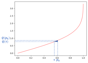
Figure 8: Illustration of ratio between $|Q^{p_{k}}-Q^{\tau}|$ and $|p_{k}-\tau|$. The red curve is a toy example quantile function of the absolute Gaussain distribution with location and scale parameters 0 and 1 respectively.

References

- Altschuler et al. (2019) Altschuler, J., Brunel, V.-E., and Malek, A. Best arm identification for contaminated bandits. Journal of Machine Learning Research, 20(91):1–39, 2019.
- Audibert et al. (2010) Audibert, J., Bubeck, S., and Munos, R. Best arm identification in multi-armed bandits. In COLT 2010 - The 23rd Conference on Learning Theory, Haifa, Israel, June 27-29, 2010, pp. 41–53. Omnipress, 2010.
- Auer et al. (2002) Auer, P., Cesa-Bianchi, N., and Fischer, P. Finite-time analysis of the multiarmed bandit problem. Machine Learning, 47(2):235–256, 2002.
- Bagnoli & Bergstrom (2005) Bagnoli, M. and Bergstrom, T. Log-concave probability and its applications. Economic Theory, 26(2):445–469, 2005. ISSN 0938-2259, 1432-0479.
- Bernstein (1924) Bernstein, S. On a modification of chebyshev’s inequality and of the error formula of laplace. Ann. Sci. Inst. Sav. Ukraine, Sect. Math, 1(4):38–49, 1924.
- Boucheron & Thomas (2012) Boucheron, S. and Thomas, M. Concentration inequalities for order statistics. Electron. Commun. Probab., 17:12 pp., 2012.
- Boucheron et al. (2013) Boucheron, S., Lugosi, G., and Massart, P. Concentration inequalities: A nonasymptotic theory of independence. Oxford university press, 2013.
- Bubeck et al. (2013) Bubeck, S., Wang, T., and Viswanathan, N. Multiple identifications in multi-armed bandits. In Proceedings of the 30th International Conference on Machine Learning, ICML 2013, Atlanta, GA, USA, 16-21 June 2013, volume 28 of JMLR Workshop and Conference Proceedings, pp. 258–265. JMLR.org, 2013.
- Cassel et al. (2018) Cassel, A., Mannor, S., and Zeevi, A. A general approach to multi-armed bandits under risk criteria. In Conference On Learning Theory, COLT 2018, Stockholm, Sweden, 6-9 July 2018, volume 75 of Proceedings of Machine Learning Research, pp. 1295–1306. PMLR, 2018.
- Cunningham et al. (2016) Cunningham, A. L., Garçon, N., Leo, O., Friedland, L. R., Strugnell, R., Laupèze, B., Doherty, M., and Stern, P. Vaccine development: From concept to early clinical testing. Vaccine, 34(52):6655–6664, 2016. ISSN 0264-410X. doi: 10.1016/j.vaccine.2016.10.016.
- David (2003) David, H. A. Order statistics. J. Wiley, 2003. ISBN 978-0-471-02723-2. OCLC: 301102741.
- David & Shimkin (2016) David, Y. and Shimkin, N. Pure Exploration for Max-Quantile Bandits. In Machine Learning and Knowledge Discovery in Databases, volume 9851, pp. 556–571. Springer International Publishing, 2016.
- David et al. (2018) David, Y., Szörényi, B., Ghavamzadeh, M., Mannor, S., and Shimkin, N. PAC bandits with risk constraints. In ISAIM, 2018.
- Dvoretzky et al. (1956) Dvoretzky, A., Kiefer, J., and Wolfowitz, J. Asymptotic minimax character of the sample distribution function and of the classical multinomial estimator. Ann. Math. Statist., 27(3):642–669, 1956. doi: 10.1214/aoms/1177728174.
- Even-Dar et al. (2006) Even-Dar, E., Mannor, S., and Mansour, Y. Action elimination and stopping conditions for the multi-armed bandit and reinforcement learning problems. Journal of machine learning research, 7(Jun):1079–1105, 2006.
- Hoeffding (1994) Hoeffding, W. Probability inequalities for sums of bounded random variables. In The Collected Works of Wassily Hoeffding, pp. 409–426. Springer, 1994.
- Howard & Ramdas (2019) Howard, S. R. and Ramdas, A. Sequential estimation of quantiles with applications to A/B-testing and best-arm identification. arXiv:1906.09712, 2019.
- Kandasamy et al. (2018) Kandasamy, K., Krishnamurthy, A., Schneider, J., and Póczos, B. Parallelised bayesian optimisation via thompson sampling. In International Conference on Artificial Intelligence and Statistics, AISTATS 2018, 9-11 April 2018, Playa Blanca, Lanzarote, Canary Islands, Spain, volume 84 of Proceedings of Machine Learning Research, pp. 133–142. PMLR, 2018.
- Kolla et al. (2019) Kolla, R. K., L.a., P., P. Bhat, S., and Jagannathan, K. Concentration bounds for empirical conditional value-at-risk: The unbounded case. Operations Research Letters, 47(1):16–20, 2019.
- Lattimore & Szepesvári (2020) Lattimore, T. and Szepesvári, C. Bandit Algorithms. Cambridge University Press, 2020. doi: 10.1017/9781108571401.
- Ledoux (2001) Ledoux, M. The concentration of measure phenomenon. American Mathematical Soc., 2001.
- Libin et al. (2017) Libin, P., Verstraeten, T., Roijers, D. M., Grujic, J., Theys, K., Lemey, P., and Nowé, A. Bayesian best-arm identification for selecting influenza mitigation strategies. CoRR, abs/1711.06299, 2017.
- Massart (2000) Massart, P. Some applications of concentration inequalities to statistics. In Annales de la Faculté des sciences de Toulouse: Mathématiques, 2000.
- Szörényi et al. (2015) Szörényi, B., Busa-Fekete, R., Weng, P., and Hüllermeier, E. Qualitative multi-armed bandits: A quantile-based approach. In Proceedings of the 32nd International Conference on Machine Learning, ICML 2015, Lille, France, 6-11 July 2015, volume 37 of JMLR Workshop and Conference Proceedings, pp. 1660–1668. JMLR.org, 2015.
- Torossian et al. (2019) Torossian, L., Garivier, A., and Picheny, V. X-armed bandits: Optimizing quantiles, cvar and other risks. In Asian Conference on Machine Learning, pp. 252–267. PMLR, 2019.
- Tran-Thanh & Yu (2014) Tran-Thanh, L. and Yu, J. Y. Functional Bandits. arXiv:1405.2432 [cs, stat], 2014. arXiv: 1405.2432.
- Yu & Nikolova (2013) Yu, J. Y. and Nikolova, E. Sample complexity of risk-averse bandit-arm selection. In IJCAI 2013, Proceedings of the 23rd International Joint Conference on Artificial Intelligence, Beijing, China, August 3-9, 2013, pp. 2576–2582. IJCAI/AAAI, 2013.
- Zielinski (2004) Zielinski, R. Optimal Quantile Estimators Small Sample Approach. Polish Academy of Sciences. Institute of Mathematics, 2004.