TLGAN: document Text Localization using Generative Adversarial Nets

Abstract

Text localization from the digital image is the first step for the optical character recognition task. Conventional image processing based text localization performs adequately for specific examples. Yet, a general text localization are only archived by recent deep-learning based modalities. Here we present document Text Localization Generative Adversarial Nets (TLGAN) which are deep neural networks to perform the text localization from digital image. TLGAN is an versatile and easy-train text localization model requiring a small amount of data. Training only ten labeled receipt images from Robust Reading Challenge on Scanned Receipts OCR and Information Extraction (SROIE), TLGAN achieved $99.83\%$ precision and $99.64\%$ recall for SROIE test data. Our TLGAN is a practical text localization solution requiring minimal effort for data labeling and model training and producing a state-of-art performance.

Keywords Deep learning  $\cdot$ Generative adversarial network  $\cdot$ Image processing  $\cdot$ optical character recognition  $\cdot$ computer vision

1 Introduction

In enterprise business, printed documents are a major communication tool. These papers are often acquired using optical devices like scanners or cameras and the data are compressed/stored as digital images. Such document images contain valuable information and there is a big need to make digital images to interpretable text. Optical character recognition (OCR) is a method to translate the printed document to digital text. OCR processes are to localize text in images following by text recognition at loci [1]. Further text/language processes may be added as needs. The text localization task is to detect texts from digital images which may contain not only texts but also graphics, drawings, lines, and noises. Conventional image processing techniques can be applied and works for specific examples, yet, such approaches are vulnerable to the real-world noises which may not be described or may not be able to describe at the processing algorithm.

Recent advances in deep learning show a great success in object detection. There are two major approaches for the object detection: region proposal network (RPN) and semantic segmentation. RPN searches object boundary coordinates, i.e. regions of interest (ROIs), and is successfully demonstrated by faster region proposal CNN (Faster-RCNN) [2], single shot multibox detector (SSD) [3], you only look once (YOLO) [4] with their successors [5, 6, 7, 8, 9]. The RPN based object detection modalities has been fine-tuned for text detection tasks, e.g. TextBoxes [10], fully-convolutional regression network (FCRN) [11], efficient and accurate scene text detector (EAST) [12] and more. Semantic segmentation produces segmentation map corresponding to the object locations and shapes. Fully convolutional networks (FCN) [13], U-Net [14] with following approaches [15, 16, 17, 18] et cetera are examples. Semantic segmentation approaches has been adopted and modified for the text detection and certainly has become a powerful text detection tool. Semantic segmentation based text detectors such as character region awareness for text detection (CRAFT) [19], multi oriented corner text detectors [20], pixel aggregation network (PANNet) [21], and connectionist text proposal network (CTPN) [22] are top ranked at robust reading competition of focused scene text (FST) and scanned receipt OCR (SROIE) [23, 24, 25]. Certainly, PANNet and CTPN used ImageNet pretrained VGG network [26, 27] for feature extraction from text contained images and the both models show great performances [23, 24, 25].

Generative adversarial network (GAN) is a framework to train a deep learning model using an adversarial processes [28]. Several GAN models have devised and, especially, GAN shows brilliant results for image-to-image translation problem, e.g. creating semantic segmentation from image or the reverse, drawing to photo translation, enhancing image resolution and more [29, 30, 31, 32]. Recent studies found GAN for the object detection from images and show superior and versatile object detection performance [33, 34, 35].

Here we introduce a document text localization generative adversarial network (TLGAN), which is a GAN specially designed for detecting text location in document images. TLGAN follows the semantic segmentation based text localization approach [19, 20, 21, 22] and estimates precise text location using a generator network structuring in a set of residual convolutional layers [31, 36, 37, 38, 39]. Effective text location estimation is carried out using Imagenet pretrained VGG network [26, 27] and TLGAN uses VGG as discriminator loss evaluation function rather than feature extraction unit for semantic segmentation [31, 21, 22]. TLGAN, therefore, take benefits of VGG’s great feature extractions without having large VGG computation in addition to versatile performance of an adversarial learning process [33, 34, 35]. TLGAN achieved $99.83\%$ precision and $99.64\%$ recall for reading challenge on Scanned Receipts OCR and Information Extraction (SROIE). Notably, we found TLGAN learned text location with a samll set of data, i.e. ten labeled images are enough to reproduce similar performance at SROIE dataset. Our TLGAN is a practical text localization solution requiring minimal effort for data labeling and model training and producing a state-of-art performance.

2 Methods

Document Text Localization Generative Adversarial Nets (TLGAN) aims to perform text localization from a text-containing image $I^{R}$ (Fig. 1a) by estimating a text localization map $I^{M}$ (Fig. 1b). Here we first address the formation of text localization map $I^{M}$ (section 2.1) and TLGAN architecture (section 2.2) followed by text localization approach (section 2.4 and Fig. 1c). We next show the training and evaluation strategies of the model used in the manuscript in sections 2.5 and 2.5.

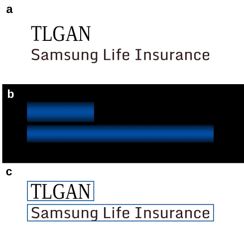
Figure 1: An example of (a) text image and corresponding (b) text localization map (colored in blue) and (c) text localization result (blue boxes).

2.1 Text localization map

Let we have an image $I^{R}$ containing $n$ text positioning at $\vec{P}_{n},n=0,...,N$. A cylindrical Gaussian map image $\vec{M}$ is given:

$$M(mx,my)=\frac{1}{2\pi\sigma_{my}}e^{-my^{2}/2\sigma_{my}^{2}},$$ (1)

where $\sigma_{my}$ denote the width of the cylindrical Gaussian map, $(mx,my)\in\mathbb{R}^{2}$.

The text locations are marked in $I^{M}$ by wrapping a cylindrical Gaussian maps $\vec{M}$ into each text position $\vec{P}_{n}$ into $I^{M}$ using a set of affine transformations [19],

$$I^{M}=\sum^{N}_{n=1}\vec{P}_{n}=\sum^{N}_{n=1}\left(A_{n}\cdot\vec{M}+\vec{b}_{n}\right),\qquad n=0,1,2,...,N.$$ (2)

Figure 1b shows an example text localization map corresponding to the text image in figure 1a.

2.2 TLGAN

A convolutional neural network (CNN) $G_{p_{g}}$ parameterized by $p_{g}$ is devised to estimate a text localization map $I^{M}$ from a text-containing image $I^{R}$:

$$G_{p_{g}}:I^{R}\mapsto I^{M},$$ (3)

where $p_{g}$ denotes a set of weights and biases in deep neural nets. We find the $\hat{p}_{g}$ by solving the equation 4 over $K$ training images $I^{R}$ and the corresponding maps $I^{M}$:

$$\hat{p}_{g}=\operatorname*{arg\,min}_{p_{g}}\frac{1}{K}\sum^{K}_{k=1}l^{M}(G_{p_{g}}(I^{R}),I^{M}).$$ (4)

From equation 4, $l^{M}$ is a loss function defined:

$$l^{M}=\frac{1}{J}\sum_{j}^{J}\left(q\times(I^{M}_{j}-G_{p_{g}}(I^{R})_{j})^{2}+r\times(\phi(I^{M})_{j}-\phi(G_{p_{g}}(I^{R}))_{j})^{2}\right),\quad j=0,1,2,...,J$$ (5)

where $j$ denotes $J$ pixels in the image, $q$ and $r$ denote the weights of the loss contents, $\phi$ is a feature extraction function which is a inter-layer feature output from a pretrained CNN, e.g. VGG19 [27] ImageNet pretrained [31, 40, 39, 41, 42].

Here we utilized a CNN network $D_{p_{d}}$ parameterized by $p_{d}$ following generative adversarial nets (GAN) [28]. Note we are following the successful work of SR-GAN by Ledig et al. [31]. Both $G_{p_{g}}$ and $D_{p_{d}}$ are CNNs and the detailed architecture of the networks are shown in Supplementary Information A.1. Briefly, $G_{p_{g}}$ takes input image $I^{R}$ and consists of stacks of residual blocks which composed by convolutional layers, batch normalization layers, and parametric ReLU activation layers [36, 37, 38, 39]. The features from residual blocks are computed using a $s$ strided convolution layer. The output $I^{M}$ is given by a fianl convolution layer with $\tanh$ activation. $D_{p_{d}}$ is a convolutional neural network to discriminate $I^{M}$ to $\hat{I^{M}}=G_{p_{g}}(I^{R})$ and is composed by a set of convolution blocks with a convolution layer, batch normalization layer and leaky ReLU activation layer [43]. A final dense layer with the sigmoid activation makes discrimination between $I^{M}$ to $\hat{I^{M}}$ using features from convolution blocks.

To find $\hat{G}_{p_{g}}$, $G_{p_{g}}$ and $D_{p_{d}}$ are optimized alternately by solving min-max problem in equation 6 [28]:

$$\min_{p_{g}}\max_{p_{d}}\mathbb{E}_{I^{M}}\left(\log D_{p_{d}}(I^{M})\right)+\mathbb{E}_{I^{R}}\left(\log-D_{p_{d}}(G_{p_{g}}(I^{R})\right).$$ (6)

2.3 Image preprocessing and post processing

Images were resized and their intensities are adjusted for train and test. We first detect a content region of the image which is the area containing information rather empty space. The content area is computed by summing the pixel intensities over x and y axis and by finding front and back edges of the signal assuming the contents exist in a rectangular region. The images are resized at the certain content region size, i.e. 550 pixels in short axis for the data set used in section 3.1. Image intensities between its 50% and 99.95% of the maximum value were mapped to the value between 0 and 255. The scaled images were processed by inferencing a trained TLGAN model. The inference output is scaled back to the original image size via the bicubic interpolation followed by the text localization described in secion 2.4.

2.4 Text localization

Trained CNN $G_{p_{g}}$ generates a text localization map $\hat{I^{M}}$ described in section 2.1. The $\hat{I^{M}}$ annotates text locations as a set of cylindrical Gaussian maps shown in figure 1b. Image segmentation over $\hat{I^{M}}$ were performed using a simple threshold followed by morphological image processes of the dilation and the border following method [44, 19]. Rectangular bounding boxes were found from the segmented images (figure 1c).

2.5 Training details and parameters

All the models were trained on machines configured with an Intel Xeon W-2135 CPU and a NVIDIA GTX 1080 Ti GPU. TLGAN model $G_{pg}$ was constructed with a convolution layer stride $s=4$ and loss parameters $q=1$ and $r=0.001$ in equation 5 (see section 2.2). Models were optimzied using the Adam optimizer with learning rate $\alpha=0.0002$, $\beta_{1}=0.5$, $\beta_{2}=0.999$ and $\epsilon=10^{-7}$ [45]. All the models, training and inference were implemented and tested using Tensorflow (https://www.tensorflow.org/) version 2.4.0 and Python version 3.6.10 with Ubuntu version 18.04.5 LTS.

3 Experiments

3.1 Benchmark dataset and model

A set of experiments were performed using Robust Reading Challenge on Scanned Receipts OCR and Information Extraction (SROIE) dataset by International Conference on Document Analysis and Recognition (ICDAR) [25]. $626$ and $361$ scanned receipt images with text bounding box annotations were given from ICDAR SROIE for training and test, subsequently. A TLGAN model was trained using the training dataset provided from SROIE. Images in training dataset were randomly cropped (augmented) $600$ times in the size of $128\times 128$ pixels on its width and height due to the limited graphic memory on our system. The TLGAN model was trained using $62,600$ augmented images. The data were randomly sampled in batch size 8 and the model was trained over $120,000$ mini-batches. The training hyper-parameters were given in section 2.5.

Experimental results from TLGAN were evaluated by following SROIE evaluation protocol and SROIE evaluation software [25, 23]. Briefly, SROIE evaluation protocol is implemented based on DetEval [46]. The SROIE evaluation program computes the mean average precision and the average recall based on F1 score [47]. H-mean score is defined by the average of the mean average precision and the average recall. We refer the results of ICDAR SROIE website (https://rrc.cvc.uab.es/?ch=13&com=evaluation&task=1) accessed at Oct., 19, 2020 to make the comparison table in table 1 [25].

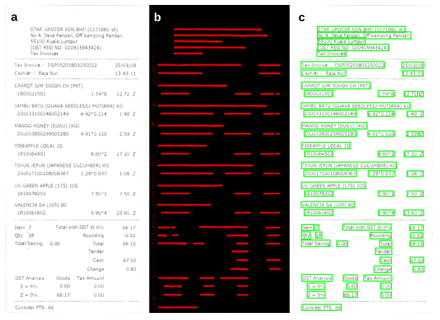
Figure 2: An example of (a) a scanned receipt image from SROIE and corresponding (b) text localization map generated using a TLGAN model. (c) text localization result presented in green boxes.

3.2 Results

Figure 2 shows an example of text localization of a SROIE data predicted using a TLGAN model. A TLGAN model generated a text localization map (figure 2b) from a preprocessed image of figure 2a, and the text locations were identified via localization process (figure 2c). The TLGAN model was tested using the SROIE task1 test dataset and the model outperformed by achieving $99.83\%$ precision, $99.64\%$ recall, and $99.23\%$ hmean (see table 1). The TLGAN consists of 1.45 million parameters (see supplementary table A.1) which is much smaller than image classification networks such as a VGG16 (138M, [27]) and a ResNet (25M, [38]). Besides its performances and sizes, we found the TLGAN models were trained easily that the model training is saturated after few thousand epochs. We hypothesised that the TLGAN model learns text localization features only with few labeled images. To verify this, we conducted a set of experiments in section 3.3 making TLGAN models with subsets of training data.

Table 1: Experimental results of TLGAN and others for SROIE taks 1, 2020-10-19 accessed [24].

Rank	Date	Method	Recall	Precision	Hmean	Ref.
-	2020-10-19	TLGAN (ours)	99.64%	99.83%	99.91%
1	2020-08-10	BOE_AIoT_CTO	98.76%	98.92%	98.84%	[21, 20]
2	2019-04-22	SCUT-DLVC-Lab-Refinement	98.64%	98.53%	98.59%	N.A.
3	2019-04-22	Ping An Property & Casualty Insurance	98.60%	98.40%	98.50%	[48, 12, 49]
4	2019-04-22	H&H Lab	97.93%	97.95%	97.94%	[20, 12]
5	2020-09-27	Only PAN	96.51%	96.80%	96.66%	[21]
6	2019-04-22	GREAT-OCR Shanghai University	96.62%	96.21%	96.42%	[50, 51]
7	2019-04-23	BOE_IOT_AIBD	95.95%	95.99%	95.97%	[9]
8	2019-04-23	EM_ocr	95.85%	96.08%	95.97%	N.A.
9	2019-05-10	Clova OCR	96.04%	95.79%	95.92%	N.A.
10	2019-04-21	IFLYTEK-textDet_v3	93.77%	95.89%	94.81%	[22]

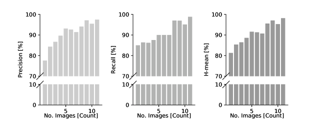
Figure 3: SROIE evaluation results from TLGAN model trained by $n$ labeled images, $n=1,2,...,11$. Precision, recall and H-mean shows from left to right panels, subsequently.

3.3 Experiments with a subset of training data

A set of TLGAN models were trained using subsets of training data, i.e. eleven images $I_{n},n=1,2,...,11$ were randomly sampled from the training dataset of ICDAR SROIE, and ten TLGAN models $G_{n},n=1,2,...,11$ were trained by sampling $n$ images followed by preprocessing described in sections 2.3 and 2.5. Figure 3 shows results from eleven TLGAN models tested using ICDAR SROIE test dataset. The test precision and recall is over $90\%$ hmean at a TLGAN model trained with only five labeled images. Further, the TLGAN model trained with 11 images almost reached to the state-of-art scores ($97\%$ hmean). For document detection tasks, our TLGAN model needs minimal amount of training data significantly reducing the data labeling works.

4 Discussions

TLGAN is a deep learning model to detect text in document and is trained using a generative adversarial network (GAN) approach. A generator network in the TLGAN model finds the text location by translating a scanned document image into a text localization map followed by finding text bounding boxes from the map (figure 1). To train a generator model, a discriminator network and a feature extraction network forms adversarial losses to find both image contents and features. A TLGAN model was trained for ICDAR SROIE task 1 dataset [24] and recorded $99.83\%$ precision, $99.64\%$ recall, and $99.23\%$ hmean (table 1). Further, we found TLGAN learns TLGAN location easily that having ten labeled document images make good text detection model with TLGAN approach. Also, the TLGAN generator network used in the manuscript is defined using 1.45M parameter, which is smaller than many other image processing networks.

The TLGAN uses image features from a ImageNet pretrained VGG19 network as an adversarial loss. The effective TLGAN feature extraction from a VGG network is successfully demonstrated [26, 27] and the pretrained VGG network is used as a part of their model. Here, we rather uses the large VGG model (e.g. VGG16 with 138M parameters) but indirectly added in to a adversarial loss in addition to the mean-square-error loss. We found the TLGAN rapidly learns text location specific features from a pretrained VGG network devoiding an expensive computation of a VGG network. Such a knowledge transfer may allow the TLGAN not only to learn the text location map fast but also to need a small set of training data.

The current implementation of the TLGAN has following limitations. First, the generator network of TLGAN follows residual convolutional network design [31, 36, 37, 38, 39] and it certainly helps on a stable adversarial learning [31]. Yet, a residual convolutions with $3\times 3$ kernels only find the convolutional receptive field locally, therefore, the generator is limited to learn the image features at a certain size. In other words, the text contents in the image requires in specific font size and image resolution to achieve the best result with the current TLGAN implementation (see section 2.3). We found such can be solved by replacing residual convolutional layers to a U-Net like architecture [14] which forms multi-resolution features with a high-resolution image reconstruction. We certainly experience some GAN issues of vanishing gradients and mode collapse issues with a U-Net like generator in a long batch training. Here we uses VGG19 to take the feature loss from the image. Second, although this VGG network is not a part of a generator, it is a part of training and is taking a large computation and memory during the training. We tried replacing the VGG19 to the MobileNetV2 [52] which reduces the computation and memory uses during the training as well as maintains learning features similar to the VGG19. This certainly a better option in practice to have larger batches at the training. Third, the generator in TLGAN only has 1.45M parameters, yet the model solves pixel to pixel problem and computation is expensive. In addition, the ROI proposal computation remains on CPU computation as a post processing (see section 2.3). Such a ROI proposal can be integrated within the network [2] or implementing post processing module on GPU.

TLGAN is a document text localization GAN to form a text localization map from the document image followed by the text localization. The TLGAN takes the advantages of the adversarial learning and the pretrained convolutional network of VGG and learns the text localization features rapidly and easily. TLGAN is a practical text localization model by reducing the data labeling work significantly, and can be trained readily for a new kind of datasets. Further investigations are needed to prove the benefits and limitations of the TLGAN.

Author information

Contributions

D.K. and M.K. designed the research; D.K., M.K., E.W., S.S. and J.N. performed the research; D.K. wrote the manuscript. D.K and M.K contribute the manuscript equally.

Corresponding author

Correspondence to Dongyoung Kim (dongyoung.kim@me.com; http://www.dykim.net).

Ethics declarations

Competing interests

D.K., M.K. and E.W. are inventors of the filed patents in Korea; 10-2019-0059652 (KR).

Appendix A Supplementary Tables

A.1 TLGAN generator network architectures

Layer (type)	Output Shape	Param #	Connected to
input_4 (InputLayer)	[(N, N, N)]	0
conv2d_8 (Conv2D)	multiple	15616	input_4[0][0]
activation (Activation)	multiple	0	conv2d_8[0][0]
conv2d_9 (Conv2D)	multiple	36928	activation[0][0]
activation_1 (Activation)	multiple	0	conv2d_9[0][0]
batch_normalization_7 (BatchNormalization)	multiple	256	activation_1[0][0]
conv2d_10 (Conv2D)	multiple	36928	batch_normalization_7[0][0]
batch_normalization_8 (BatchNormalization)	multiple	256	conv2d_10[0][0]
add (Add)	multiple	0	batch_normalization_8[0][0], activation[0][0]
conv2d_11 (Conv2D)	multiple	36928	add[0][0]
activation_2 (Activation)	multiple	0	conv2d_11[0][0]
batch_normalization_9 (BatchNormalization)	multiple	256	activation_2[0][0]
conv2d_12 (Conv2D)	multiple	36928	batch_normalization_9[0][0]
batch_normalization_10 (BatchNormalization)	multiple	256	conv2d_12[0][0]
add_1 (Add)	multiple	0	batch_normalization_10[0][0], add[0][0]
conv2d_13 (Conv2D)	multiple	36928	add_1[0][0]
activation_3 (Activation)	multiple	0	conv2d_13[0][0]
batch_normalization_11 (BatchNormalization)	multiple	256	activation_3[0][0]
conv2d_14 (Conv2D)	multiple	36928	batch_normalization_11[0][0]
batch_normalization_12 (BatchNormalization)	multiple	256	conv2d_14[0][0]
add_2 (Add)	multiple	0	batch_normalization_12[0][0], add_1[0][0]
conv2d_15 (Conv2D)	multiple	36928	add_2[0][0]
activation_4 (Activation)	multiple	0	conv2d_15[0][0]
batch_normalization_13 (BatchNormalization)	multiple	256	activation_4[0][0]
conv2d_16 (Conv2D)	multiple	36928	batch_normalization_13[0][0]
batch_normalization_14 (BatchNormalization)	multiple	256	conv2d_16[0][0]
add_3 (Add)	multiple	0	batch_normalization_14[0][0], add_2[0][0]
conv2d_17 (Conv2D)	multiple	36928	add_3[0][0]
activation_5 (Activation)	multiple	0	conv2d_17[0][0]
batch_normalization_15 (BatchNormalization)	multiple	256	activation_5[0][0]
conv2d_18 (Conv2D)	multiple	36928	batch_normalization_15[0][0]
batch_normalization_16 (BatchNormalization)	multiple	256	conv2d_18[0][0]
add_4 (Add)	multiple	0	batch_normalization_16[0][0], add_3[0][0]
conv2d_19 (Conv2D)	multiple	36928	add_4[0][0]
activation_6 (Activation)	multiple	0	conv2d_19[0][0]
batch_normalization_17 (BatchNormalization)	multiple	256	activation_6[0][0]
conv2d_20 (Conv2D)	multiple	36928	batch_normalization_17[0][0]
batch_normalization_18 (BatchNormalization)	multiple	256	conv2d_20[0][0]
add_5 (Add)	multiple	0	batch_normalization_18[0][0], add_4[0][0]
conv2d_21 (Conv2D)	multiple	36928	add_5[0][0]
activation_7 (Activation)	multiple	0	conv2d_21[0][0]
batch_normalization_19 (BatchNormalization)	multiple	256	activation_7[0][0]
conv2d_22 (Conv2D)	multiple	36928	batch_normalization_19[0][0]
batch_normalization_20 (BatchNormalization)	multiple	256	conv2d_22[0][0]
add_6 (Add)	multiple	0	batch_normalization_20[0][0], add_5[0][0]
conv2d_23 (Conv2D)	multiple	36928	add_6[0][0]
activation_8 (Activation)	multiple	0	conv2d_23[0][0]
batch_normalization_21 (BatchNormalization)	multiple	256	activation_8[0][0]
conv2d_24 (Conv2D)	multiple	36928	batch_normalization_21[0][0]
batch_normalization_22 (BatchNormalization)	multiple	256	conv2d_24[0][0]

Layer (type)	Output Shape	Param #	Connected to
add_7 (Add)	multiple	0	batch_normalization_22[0][0], add_6[0][0]
conv2d_25 (Conv2D)	multiple	36928	add_7[0][0]
activation_9 (Activation)	multiple	0	conv2d_25[0][0]
batch_normalization_23 (BatchNormalization)	multiple	256	activation_9[0][0]
conv2d_26 (Conv2D)	multiple	36928	batch_normalization_23[0][0]
batch_normalization_24 (BatchNormalization)	multiple	256	conv2d_26[0][0]
add_8 (Add)	multiple	0	batch_normalization_24[0][0], add_7[0][0]
conv2d_27 (Conv2D)	multiple	36928	add_8[0][0]
activation_10 (Activation)	multiple	0	conv2d_27[0][0]
batch_normalization_25 (BatchNormalization)	multiple	256	activation_10[0][0]
conv2d_28 (Conv2D)	multiple	36928	batch_normalization_25[0][0]
batch_normalization_26 (BatchNormalization)	multiple	256	conv2d_28[0][0]
add_9 (Add)	multiple	0	batch_normalization_26[0][0], add_8[0][0]
conv2d_29 (Conv2D)	multiple	36928	add_9[0][0]
activation_11 (Activation)	multiple	0	conv2d_29[0][0]
batch_normalization_27 (BatchNormalization)	multiple	256	activation_11[0][0]
conv2d_30 (Conv2D)	multiple	36928	batch_normalization_27[0][0]
batch_normalization_28 (BatchNormalization)	multiple	256	conv2d_30[0][0]
add_10 (Add)	multiple	0	batch_normalization_28[0][0], add_9[0][0]
conv2d_31 (Conv2D)	multiple	36928	add_10[0][0]
activation_12 (Activation)	multiple	0	conv2d_31[0][0]
batch_normalization_29 (BatchNormalization)	multiple	256	activation_12[0][0]
conv2d_32 (Conv2D)	multiple	36928	batch_normalization_29[0][0]
batch_normalization_30 (BatchNormalization)	multiple	256	conv2d_32[0][0]
add_11 (Add)	multiple	0	batch_normalization_30[0][0], add_10[0][0]
conv2d_33 (Conv2D)	multiple	36928	add_11[0][0]
activation_13 (Activation)	multiple	0	conv2d_33[0][0]
batch_normalization_31 (BatchNormalization)	multiple	256	activation_13[0][0]
conv2d_34 (Conv2D)	multiple	36928	batch_normalization_31[0][0]
batch_normalization_32 (BatchNormalization)	multiple	256	conv2d_34[0][0]
add_12 (Add)	multiple	0	batch_normalization_32[0][0], add_11[0][0]
conv2d_35 (Conv2D)	multiple	36928	add_12[0][0]
activation_14 (Activation)	multiple	0	conv2d_35[0][0]
batch_normalization_33 (BatchNormalization)	multiple	256	activation_14[0][0]
conv2d_36 (Conv2D)	multiple	36928	batch_normalization_33[0][0]
batch_normalization_34 (BatchNormalization)	multiple	256	conv2d_36[0][0]
add_13 (Add)	multiple	0	batch_normalization_34[0][0], add_12[0][0]
conv2d_37 (Conv2D)	multiple	36928	add_13[0][0]
activation_15 (Activation)	multiple	0	conv2d_37[0][0]
batch_normalization_35 (BatchNormalization)	multiple	256	activation_15[0][0]
conv2d_38 (Conv2D)	multiple	36928	batch_normalization_35[0][0]
batch_normalization_36 (BatchNormalization)	multiple	256	conv2d_38[0][0]
add_14 (Add)	multiple	0	batch_normalization_36[0][0], add_13[0][0]
conv2d_39 (Conv2D)	multiple	36928	add_14[0][0]
activation_16 (Activation)	multiple	0	conv2d_39[0][0]
batch_normalization_37 (BatchNormalization)	multiple	256	activation_16[0][0]
conv2d_40 (Conv2D)	multiple	36928	batch_normalization_37[0][0]
batch_normalization_38 (BatchNormalization)	multiple	256	conv2d_40[0][0]
add_15 (Add)	multiple	0	batch_normalization_38[0][0], add_14[0][0]
conv2d_41 (Conv2D)	multiple	36928	add_15[0][0]
batch_normalization_39 (BatchNormalization)	multiple	256	conv2d_41[0][0]
add_16 (Add)	multiple	0	batch_normalization_39[0][0], activation[0][0]
conv2d_42 (Conv2D)	multiple	147712	add_16[0][0]
activation_17 (Activation)	multiple	0	conv2d_42[0][0]
conv2d_43 (Conv2D)	multiple	62211	activation_17[0][0]
Total params		1,452,611
Trainable params		1,448,387
Non-trainable params		4,224

A.2 TLGAN discriminator network architectures

Layer (type)	Output Shape	Param #
input_3 (InputLayer)	[(None, 64, 64, 3)]	0
conv2d (Conv2D)	(None, 64, 64, 64)	1792
leaky_re_lu (LeakyReLU)	(None, 64, 64, 64)	0
conv2d_1 (Conv2D)	(None, 32, 32, 64)	36928
leaky_re_lu_1 (LeakyReLU)	(None, 32, 32, 64)	0
batch_normalization (BatchNormalization)	(None, 32, 32, 64)	256
conv2d_2 (Conv2D)	(None, 32, 32, 128)	73856
leaky_re_lu_2 (LeakyReLU)	(None, 32, 32, 128)	0
batch_normalization_1 (BatchNormalization)	(None, 32, 32, 128)	512
conv2d_3 (Conv2D)	(None, 16, 16, 128)	147584
leaky_re_lu_3 (LeakyReLU)	(None, 16, 16, 128)	0
batch_normalization_2 (BatchNormalization)	(None, 16, 16, 128)	512
conv2d_4 (Conv2D)	(None, 16, 16, 256)	295168
leaky_re_lu_4 (LeakyReLU)	(None, 16, 16, 256)	0
batch_normalization_3 (BatchNormalization)	(None, 16, 16, 256)	1024
conv2d_5 (Conv2D)	(None, 8, 8, 256)	590080
leaky_re_lu_5 (LeakyReLU)	(None, 8, 8, 256)	0
batch_normalization_4 (BatchNormalization)	(None, 8, 8, 256)	1024
conv2d_6 (Conv2D)	(None, 8, 8, 512)	1180160
leaky_re_lu_6 (LeakyReLU)	(None, 8, 8, 512)	0
batch_normalization_5 (BatchNormalization)	(None, 8, 8, 512)	2048
conv2d_7 (Conv2D)	(None, 4, 4, 512)	2359808
leaky_re_lu_7 (LeakyReLU)	(None, 4, 4, 512)	0
batch_normalization_6 (BatchNormalization)	(None, 4, 4, 512)	2048
dense (Dense)	(None, 4, 4, 1024)	525312
leaky_re_lu_8 (LeakyReLU)	(None, 4, 4, 1024)	0
dense_1 (Dense)	(None, 4, 4, 1)	1025
Total params		5,219,137
Trainable params		0
Non-trainable params		5,219,137

A.3 TLGAN feature extraction network architectures (VGG19)

Layer (type)	Output Shape	Param #
input_1 (InputLayer)	[(None, 64, 64, 3)]	0
block1_conv1 (Conv2D)	(None, 64, 64, 64)	1792
block1_conv2 (Conv2D)	(None, 64, 64, 64)	36928
block1_pool (MaxPooling2D)	(None, 32, 32, 64)	0
block2_conv1 (Conv2D)	(None, 32, 32, 128)	73856
block2_conv2 (Conv2D)	(None, 32, 32, 128)	147584
block2_pool (MaxPooling2D)	(None, 16, 16, 128)	0
block3_conv1 (Conv2D)	(None, 16, 16, 256)	295168
block3_conv2 (Conv2D)	(None, 16, 16, 256)	590080
block3_conv3 (Conv2D)	(None, 16, 16, 256)	590080
Total params		1,735,488
Trainable params		0
Non-trainable params		1,735,488

References

- [1] A. P. Tafti, A. Baghaie, M. Assefi, H. R. Arabnia, Z. Yu, and P. Peissig, “OCR as a Service: An Experimental Evaluation of Google Docs OCR, Tesseract, ABBYY FineReader, and Transym,” 2016, pp. 735–746. [Online]. Available: http://link.springer.com/10.1007/978-3-319-50835-1{_}66
- [2] S. Ren, K. He, R. Girshick, and J. Sun, “Faster R-CNN: Towards Real-Time Object Detection with Region Proposal Networks,” jun 2015. [Online]. Available: http://arxiv.org/abs/1506.01497
- [3] W. Liu, D. Anguelov, D. Erhan, C. Szegedy, S. Reed, C.-Y. Fu, and A. C. Berg, “SSD: Single Shot MultiBox Detector,” dec 2015. [Online]. Available: http://arxiv.org/abs/1512.02325http://dx.doi.org/10.1007/978-3-319-46448-0{_}2
- [4] J. Redmon, S. Divvala, R. Girshick, and A. Farhadi, “You Only Look Once: Unified, Real-Time Object Detection,” jun 2015. [Online]. Available: http://arxiv.org/abs/1506.02640
- [5] J. Dai, Y. Li, K. He, and J. Sun, “R-FCN: Object Detection via Region-based Fully Convolutional Networks,” may 2016. [Online]. Available: http://arxiv.org/abs/1605.06409
- [6] J. Redmon and A. Farhadi, “YOLO9000: Better, Faster, Stronger,” dec 2016. [Online]. Available: http://arxiv.org/abs/1612.08242
- [7] T.-Y. Lin, P. Dollár, R. Girshick, K. He, B. Hariharan, and S. Belongie, “Feature Pyramid Networks for Object Detection,” dec 2016. [Online]. Available: http://arxiv.org/abs/1612.03144
- [8] C.-Y. Fu, W. Liu, A. Ranga, A. Tyagi, and A. C. Berg, “DSSD : Deconvolutional Single Shot Detector,” jan 2017. [Online]. Available: http://arxiv.org/abs/1701.06659
- [9] J. Redmon and A. Farhadi, “YOLOv3: An Incremental Improvement,” apr 2018. [Online]. Available: http://arxiv.org/abs/1804.02767
- [10] M. Liao, B. Shi, X. Bai, X. Wang, and W. Liu, “TextBoxes: A Fast Text Detector with a Single Deep Neural Network,” nov 2016. [Online]. Available: http://arxiv.org/abs/1611.06779
- [11] A. Gupta, A. Vedaldi, and A. Zisserman, “Synthetic Data for Text Localisation in Natural Images,” apr 2016. [Online]. Available: http://arxiv.org/abs/1604.06646
- [12] X. Zhou, C. Yao, H. Wen, Y. Wang, S. Zhou, W. He, and J. Liang, “EAST: An Efficient and Accurate Scene Text Detector,” apr 2017. [Online]. Available: http://arxiv.org/abs/1704.03155
- [13] J. Long, E. Shelhamer, and T. Darrell, “Fully Convolutional Networks for Semantic Segmentation,” nov 2014. [Online]. Available: http://arxiv.org/abs/1411.4038
- [14] O. Ronneberger, P. Fischer, and T. Brox, “U-Net: Convolutional Networks for Biomedical Image Segmentation,” may 2015. [Online]. Available: http://arxiv.org/abs/1505.04597
- [15] F. Yu and V. Koltun, “Multi-Scale Context Aggregation by Dilated Convolutions,” nov 2015. [Online]. Available: http://arxiv.org/abs/1511.07122
- [16] M. Drozdzal, E. Vorontsov, G. Chartrand, S. Kadoury, and C. Pal, “The Importance of Skip Connections in Biomedical Image Segmentation,” aug 2016. [Online]. Available: http://arxiv.org/abs/1608.04117
- [17] S. Jégou, M. Drozdzal, D. Vazquez, A. Romero, and Y. Bengio, “The One Hundred Layers Tiramisu: Fully Convolutional DenseNets for Semantic Segmentation,” nov 2016. [Online]. Available: http://arxiv.org/abs/1611.09326
- [18] D. Kim, Y. Min, J. M. Oh, and Y.-K. Cho, “AI-powered transmitted light microscopy for functional analysis of live cells,” Scientific Reports, vol. 9, no. 1, p. 18428, dec 2019. [Online]. Available: https://doi.org/10.1038/s41598-019-54961-xhttp://www.nature.com/articles/s41598-019-54961-x
- [19] Y. Baek, B. Lee, D. Han, S. Yun, and H. Lee, “Character Region Awareness for Text Detection,” Proceedings of the IEEE Computer Society Conference on Computer Vision and Pattern Recognition, vol. 2019-June, pp. 9357–9366, apr 2019. [Online]. Available: http://arxiv.org/abs/1904.01941
- [20] P. Lyu, C. Yao, W. Wu, S. Yan, and X. Bai, “Multi-Oriented Scene Text Detection via Corner Localization and Region Segmentation,” Proceedings of the IEEE Computer Society Conference on Computer Vision and Pattern Recognition, pp. 7553–7563, feb 2018. [Online]. Available: http://arxiv.org/abs/1802.08948
- [21] W. Wang, E. Xie, X. Song, Y. Zang, W. Wang, T. Lu, G. Yu, and C. Shen, “Efficient and Accurate Arbitrary-Shaped Text Detection with Pixel Aggregation Network,” Proceedings of the IEEE International Conference on Computer Vision, vol. 2019-Octob, pp. 8439–8448, aug 2019. [Online]. Available: http://arxiv.org/abs/1908.05900
- [22] Z. Tian, W. Huang, T. He, P. He, and Y. Qiao, “Detecting Text in Natural Image with Connectionist Text Proposal Network,” 2016, pp. 56–72. [Online]. Available: http://link.springer.com/10.1007/978-3-319-46484-8{_}4
- [23] D. Karatzas, F. Shafait, S. Uchida, M. Iwamura, L. G. I. Bigorda, S. R. Mestre, J. Mas, D. F. Mota, J. A. Almazan, and L. P. de las Heras, “ICDAR 2013 Robust Reading Competition,” in 2013 12th International Conference on Document Analysis and Recognition. IEEE, aug 2013, pp. 1484–1493. [Online]. Available: http://ieeexplore.ieee.org/document/6628859/
- [24] ICDAR, “Results - ICDAR 2019 Robust Reading Challenge on Scanned Receipts OCR and Information Extraction - Robust Reading Competition,” 2020. [Online]. Available: https://rrc.cvc.uab.es/?ch=13{&}com=evaluation{&}task=1
- [25] ——, “ICDAR 2019 Robust Reading Challenge on Scanned Receipts OCR and Information Extraction,” 2019. [Online]. Available: https://rrc.cvc.uab.es/?ch=13
- [26] J. Deng, W. Dong, R. Socher, L.-J. Li, Kai Li, and Li Fei-Fei, “ImageNet: A large-scale hierarchical image database,” in 2009 IEEE Conference on Computer Vision and Pattern Recognition. IEEE, jun 2009, pp. 248–255. [Online]. Available: https://ieeexplore.ieee.org/document/5206848/
- [27] K. Simonyan and A. Zisserman, “Very Deep Convolutional Networks for Large-Scale Image Recognition,” sep 2014. [Online]. Available: http://arxiv.org/abs/1409.1556
- [28] I. J. Goodfellow, J. Pouget-Abadie, M. Mirza, B. Xu, D. Warde-Farley, S. Ozair, A. Courville, and Y. Bengio, “Generative Adversarial Networks,” 2019 IEEE/CVF International Conference on Computer Vision Workshop (ICCVW), pp. 3063–3071, jun 2014. [Online]. Available: http://arxiv.org/abs/1908.08930https://ieeexplore.ieee.org/document/9022395/http://arxiv.org/abs/1406.2661
- [29] P. Luc, C. Couprie, S. Chintala, and J. Verbeek, “Semantic Segmentation using Adversarial Networks,” nov 2016. [Online]. Available: http://arxiv.org/abs/1611.08408
- [30] P. Isola, J.-Y. Zhu, T. Zhou, and A. A. Efros, “Image-to-Image Translation with Conditional Adversarial Networks,” in 2017 IEEE Conference on Computer Vision and Pattern Recognition (CVPR), vol. 2017-Janua. IEEE, jul 2017, pp. 5967–5976. [Online]. Available: http://arxiv.org/abs/1611.07004http://ieeexplore.ieee.org/document/8100115/
- [31] C. Ledig, L. Theis, F. Huszar, J. Caballero, A. Cunningham, A. Acosta, A. Aitken, A. Tejani, J. Totz, Z. Wang, and W. Shi, “Photo-Realistic Single Image Super-Resolution Using a Generative Adversarial Network,” Proceedings - 30th IEEE Conference on Computer Vision and Pattern Recognition, CVPR 2017, vol. 2017-Janua, pp. 105–114, sep 2016. [Online]. Available: http://arxiv.org/abs/1609.04802
- [32] T. Park, M.-Y. Liu, T.-C. Wang, and J.-Y. Zhu, “Semantic Image Synthesis with Spatially-Adaptive Normalization,” Proceedings of the IEEE Computer Society Conference on Computer Vision and Pattern Recognition, vol. 2019-June, pp. 2332–2341, mar 2019. [Online]. Available: http://arxiv.org/abs/1903.07291
- [33] C. D. Prakash and L. J. Karam, “It GAN DO Better: GAN-based Detection of Objects on Images with Varying Quality,” 2019. [Online]. Available: http://arxiv.org/abs/1912.01707
- [34] L. Liu, M. Muelly, J. Deng, T. Pfister, and L.-J. Li, “Generative Modeling for Small-Data Object Detection,” in 2019 IEEE/CVF International Conference on Computer Vision (ICCV), vol. 2019-Octob. IEEE, oct 2019, pp. 6072–6080. [Online]. Available: https://ieeexplore.ieee.org/document/9008794/
- [35] W. Wang, W. Hong, F. Wang, and J. Yu, “GAN-Knowledge Distillation for One-Stage Object Detection,” IEEE Access, vol. 8, pp. 60 719–60 727, 2020. [Online]. Available: https://ieeexplore.ieee.org/document/9046859/
- [36] J. Johnson, A. Alahi, and L. Fei-Fei, “Perceptual Losses for Real-Time Style Transfer and Super-Resolution,” mar 2016. [Online]. Available: http://arxiv.org/abs/1603.08155
- [37] S. Ioffe and C. Szegedy, “Batch Normalization: Accelerating Deep Network Training by Reducing Internal Covariate Shift,” feb 2015. [Online]. Available: http://arxiv.org/abs/1502.03167
- [38] K. He, X. Zhang, S. Ren, and J. Sun, “Deep Residual Learning for Image Recognition,” dec 2015. [Online]. Available: http://image-net.org/challenges/LSVRC/2015/http://arxiv.org/abs/1512.03385
- [39] W. Shi, J. Caballero, F. Huszár, J. Totz, A. P. Aitken, R. Bishop, D. Rueckert, and Z. Wang, “Real-Time Single Image and Video Super-Resolution Using an Efficient Sub-Pixel Convolutional Neural Network,” sep 2016. [Online]. Available: http://arxiv.org/abs/1609.05158
- [40] C. Dong, C. C. Loy, K. He, and X. Tang, “Image Super-Resolution Using Deep Convolutional Networks,” dec 2014. [Online]. Available: http://arxiv.org/abs/1501.00092
- [41] L. A. Gatys, A. S. Ecker, and M. Bethge, “Texture Synthesis Using Convolutional Neural Networks,” may 2015. [Online]. Available: http://arxiv.org/abs/1505.07376
- [42] J. Bruna, P. Sprechmann, and Y. LeCun, “Super-Resolution with Deep Convolutional Sufficient Statistics,” nov 2015. [Online]. Available: http://arxiv.org/abs/1511.05666
- [43] A. Radford, L. Metz, and S. Chintala, “Unsupervised Representation Learning with Deep Convolutional Generative Adversarial Networks,” nov 2015. [Online]. Available: http://arxiv.org/abs/1511.06434
- [44] S. Suzuki and K. Be, “Topological structural analysis of digitized binary images by border following,” Computer Vision, Graphics, and Image Processing, vol. 30, no. 1, pp. 32–46, apr 1985. [Online]. Available: https://linkinghub.elsevier.com/retrieve/pii/0734189X85900167
- [45] D. P. Kingma and J. Ba, “Adam: A Method for Stochastic Optimization,” 3rd International Conference on Learning Representations, ICLR 2015 - Conference Track Proceedings, pp. 1–15, dec 2014. [Online]. Available: http://arxiv.org/abs/1412.6980
- [46] C. Wolf and J.-M. Jolion, “Object count/area graphs for the evaluation of object detection and segmentation algorithms,” International Journal of Document Analysis and Recognition (IJDAR), vol. 8, no. 4, pp. 280–296, sep 2006. [Online]. Available: http://link.springer.com/10.1007/s10032-006-0014-0
- [47] M. Everingham, S. M. A. Eslami, L. Van Gool, C. K. I. Williams, J. Winn, and A. Zisserman, “The Pascal Visual Object Classes Challenge: A Retrospective,” International Journal of Computer Vision, vol. 111, no. 1, pp. 98–136, jan 2015. [Online]. Available: http://link.springer.com/10.1007/s11263-014-0733-5
- [48] S. Sun, J. Pang, J. Shi, S. Yi, and W. Ouyang, “FishNet: A Versatile Backbone for Image, Region, and Pixel Level Prediction,” jan 2019. [Online]. Available: https://arxiv.org/abs/1901.03495http://arxiv.org/abs/1901.03495
- [49] Z. Zhang, T. He, H. Zhang, Z. Zhang, J. Xie, and M. Li, “Bag of Freebies for Training Object Detection Neural Networks,” feb 2019. [Online]. Available: https://arxiv.org/abs/1902.04103http://arxiv.org/abs/1902.04103
- [50] S.-H. Gao, M.-M. Cheng, K. Zhao, X.-Y. Zhang, M.-H. Yang, and P. Torr, “Res2Net: A New Multi-scale Backbone Architecture,” apr 2019. [Online]. Available: https://arxiv.org/abs/1904.01169http://arxiv.org/abs/1904.01169http://dx.doi.org/10.1109/TPAMI.2019.2938758
- [51] W. Wang, E. Xie, X. Li, W. Hou, T. Lu, G. Yu, and S. Shao, “Shape Robust Text Detection with Progressive Scale Expansion Network,” mar 2019. [Online]. Available: https://arxiv.org/abs/1903.12473http://arxiv.org/abs/1903.12473
- [52] M. Sandler, A. Howard, M. Zhu, A. Zhmoginov, and L.-C. Chen, “MobileNetV2: Inverted Residuals and Linear Bottlenecks,” jan 2018. [Online]. Available: http://arxiv.org/abs/1801.04381
Acknowledgements
elsarticle We thank all the data analytic laboratory members at Samsung Life Insurance for their support and feedback.