Model updating after interventions paradoxically introduces bias

Abstract

Machine learning is increasingly being used to generate prediction models for use in a number of real-world settings, from credit risk assessment to clinical decision support. Recent discussions have highlighted potential problems in the updating of a predictive score for a binary outcome when an existing predictive score forms part of the standard workflow, driving interventions. In this setting, the existing score induces an additional causative pathway which leads to miscalibration when the original score is replaced. We propose a general causal framework to describe and address this problem, and demonstrate an equivalent formulation as a partially observed Markov decision process. We use this model to demonstrate the impact of such ‘naive updating’ when performed repeatedly. Namely, we show that successive predictive scores may converge to a point where they predict their own effect, or may eventually tend toward a stable oscillation between two values, and we argue that neither outcome is desirable. Furthermore, we demonstrate that even if model-fitting procedures improve, actual performance may worsen. We complement these findings with a discussion of several potential routes to overcome these issues.

Note: Sections of this preprint on ‘Successive adjuvancy’ (section 4, theorem 2, figures 4, 5, and associated discussions) were not included in the originally submitted version of this paper due to length. This material does not appear in the published version of this manuscript, and the reader should be aware that these sections did not undergo peer review.

1 Introduction

A common machine learning task concerns the prediction of an outcome $Y$ given a known set of predictors $X$ [Friedman et al., 2001]. Usually, the intent is to anticipate the value of $Y$ in situations in which only $X$ is known. Often, the ultimate goal is to avoid or encourage certain values of $Y$, with interventions guided by the predictions provided by the algorithm.

We focus on the standard setting, often seen in healthcare, where $X$ is first observed and used to make predictions about $Y$, then interventions occur before outcomes are observed. This setting can lead to prediction scores being ‘victims of their own success’ [Lenert et al., 2019, Sperrin et al., 2019]. Interventions driven by the score can change the distribution of the data and outcomes, leading to a decay in observed performance, particularly if the intervention is successful. Analysis of this effect requires consideration of the causal processes governing $X$, $Y$, and the potential interventions driven by the score [Sperrin et al., 2019]. Predictive scores are often implemented by direct dissemination to agents that are capable of modifying these causal processes [Rahimian et al., 2018, Hyland et al., 2020], which leads to vulnerability to this problem. This problem also exist if predictions influence discrete actions, initial progress for this has been made using bandits [Shi et al., 2020]. The phenomenon in which a predictive model influences its own effect has been called ‘performative prediction’ [Perdomo et al., 2020], and is of interest in model fairness [Liu et al., 2018, Elzayn et al., 2019], in that actions taken in response to a model may pervert fairness metrics under which the model was designed.

This problem is particularly critical in settings where existing predictive scores are to be replaced by an updated version. In many real-world contexts, the underlying phenomena represented by the predictive model will change over time [Wallace et al., 2014]; statistical procedures for prediction may also improve (particularly for complex tasks); and researchers may wish to include further predictors or increase the scope of predictive scores. In general, we may expect that most predictive algorithms will need to be updated or replaced over time. Up-to-date models should generally be trained on the most recent available data which, as described above, will be contaminated by interventions based on existing scores. Should a new predictive model be fitted to new observations of $X$ and $Y$, it will consequently also model the impact of the existing score. Removal of the existing score will introduce bias into predictions made by the new score, as will insertion of the new score in place of the old. We term such an operation a ‘naive model replacement’.

Our main aim is to introduce a general causal framework under which this phenomenon can be quantitatively studied. We use this framework to draw attention to the hazards of naive model replacement, especially when it occurs repeatedly. We introduce these hazards in the context of a generalised ultimate aim of the model, formulated as a constrained optimisation problem in which the occurrence of undesirable values of $Y$ is to be minimised with limited intervention. We also use our model to describe a second replacement strategy, ‘successive adjuvancy’, in which new predictive scores are ‘added’ to previous scores, with different emergent properties.

A simple parable of this phenomenon concerns yearly influenza vaccinations. In a vaccination-naive population, risk assessments for influenza motivate widespread vaccination. However, in a later ‘epoch’, the risk may appear much lower, and could naively suggest vaccination is no longer required introducing risks to public health. More generally, updated risk scores for clinical outcomes may be biased due to the interventions motivated by the scores themselves. As a second example, consider risk scores used to predict future emergency hospital admissions $Y$, on the basis of covariates $X$ [Rahimian et al., 2018]. Suppose that prescription of some drug $D\in X$ confers increased risk, and this is established by the risk score. Should such risk scores be distributed at time $t=0$ to agents able to modify these factors (e.g., doctors), they may intervene by taking patients off $D$ thereby reducing emergency admission risk $\mathbb{E}[Y]$ at a time $t=1$. If a new score is naively fitted to $X$ at $t=0$ and $Y$ at $t=1$, it would underestimate the danger of $D$.

Section 2 describes the problem in terms of causal effects. We develop this into a full model specification in Section 2.2, along with a description of the constrained optimisation problem the model/intervention pair aims to solve in 2.3. In Section 3, we analyse the short and long-term effects of repeated naive replacement and show that they are generally undesirable , and in section 4 we describe successive adjuvancy and examine long-term effects in a simplified setting. In Section 5, we discuss three classes of solutions: more complex modelling, routine maintenance of a ‘hold-out’ set, and controlled interventions. In Section 6 we describe a reformulation of the model as control theory problem. Finally, in Section 7, we discuss limitations and implications of our approach. Our supplementary material contains relevant examples and proofs, an exposition of the problem in a real-world example, and a list of open problems in this setting.

2 Model

2.1 Overview

Assume that we are attempting to predict an outcome $Y$ given a known set of covariates $X$. For simplicity, we assume $Y$ is a binary (e.g. admission versus non admission to an Intensive Care Unit) and model it as a Bernoulli random variable. If $Y=1$ is considered to be a negative outcome, often the eventual aim is to reduce $\mathbb{P}(Y=1|X)=\mathbb{E}[Y|X]$; we will discuss this in Section 2.2 once we have defined terms formally. For the moment, we assume the causal structure shown in Figure 1. We denote by $\rho_{0}(X)$ an initial predictive model for $\mathbb{E}[Y|X]$, fitted to observations of $(X,Y)$ generated under the causal structure in Figure 1A. During deployment, we compute $\rho_{0}(X)$ for all members of a population and disseminate it to agents who can intervene on $X$ (e.g. doctors) based on those predictions, aiming to prevent $Y=1$. Replacing or updating $\rho_{0}$, will typically involve fitting a new predictive model $\rho_{1}(X)$ to new observations of $(X,Y)$. It is clear that while $\rho_{0}(X)$ is an estimator of $\mathbb{E}[Y|X]$, the new predictive function $\rho_{1}(X)$ is instead an estimator of

$$\mathbb{E}\left[Y|X,\textrm{do}\left[\rho_{0}(X)\right]\right]$$ (1)

where $\textrm{do}\left[\rho_{0}(X)\right]$ indicates the action ‘compute and disseminate $\rho_{0}(X)$’. Although $\rho_{0}(X)$ is determined by $X$, the computation $\textrm{do}\left[\rho_{0}(X)\right]$ makes $\rho_{0}$ actionable. This opens a second causal pathway from $X$ to $Y$, affecting the setting in which $\rho_{1}$ is fitted (Figure 1B). If the initial score $\rho_{0}(X)$ is universally disseminated, the distribution of $Y$ given $X$ (without the $\textrm{do}\left[\rho_{0}(X)\right]$) now becomes a counterfactual which we cannot observe.

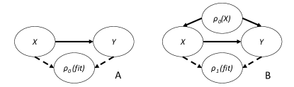
Figure 1: Causal structure under which $\rho_{0}$ (panel A) and $\rho_{1}$ (panel B) are fitted. Dashed lines indicate a model-fitting process.

2.2 General notation and assumptions

Here, we use a causal model to illustrate potential emergent behaviour resulting from repeated naive model updating, expanding out the ‘do’-operator used in section 2.1. We do not aim to cover the complexities of all real-world applications, yet our simplified setup is sufficient to demonstrate the dangers arising in this context.

As $\rho_{0}$ is deployed and drives interventions, covariate values $X$ may change, as may the dependence of $Y$ on $X$. Here, we partition $X$ into three sets:

$$X^{s} \textrm{: Fixed or `set' covariates; $\textrm{dim}(X^{s})=p^{s}$},$$

$$X^{a} \textrm{: Actionable covariates; $\textrm{dim}(X^{a})=p^{a}$},$$

$$X^{\ell} \textrm{: Latent covariates; $\textrm{dim}(X^{\ell})=p^{\ell}$}.$$ (2)

Although $X^{\ell}$ may influence the causal mechanism between $X$ and $Y$ and may be intervened on, we assume it is unobserved. Hence, only $X^{s}$ and $X^{a}$ are known when evaluating a risk score, and $X^{s}$ cannot be intervened on (e.g. ‘Age’). We also define two sets of time indicators $t,e$ (time, epoch):

$$t\in\{0,1\}: \begin{cases}t=0\textrm{: predictive score is computed}\\ t=1\textrm{: $Y$ observed, after possible}\\ \phantom{t=1:}\textrm{intervention}\end{cases}$$

$$e\in\mathbb{N}: \begin{cases}e=0\textrm{: no predictive score is used}\\ e>0\textrm{: model from epoch $e-1$ is used.}\end{cases}$$

We assume that values of $X$ depend on $t$ and $e$ using the notation $X_{e}(t)=(X^{s}_{e}(t),X^{a}_{e}(t),X^{\ell}_{e}(t))\in\Omega^{s}\times\Omega^{a}\times\Omega^{\ell}=\Omega$. As $Y$ is only observed at $t=1$, $Y$ at epoch $e$ is denoted as $Y_{e}$. At each epoch, we assume that values of $X_{e}(t)$ across individuals in the population are $iid$ with probability measure $\mu_{e}$. We introduce the following functions

$$f_{e}(x^{s},x^{a},x^{\ell}) =\mathbb{E}\left[Y_{e}|X_{e}(1)=(x^{s},x^{a},x^{\ell})\right]$$

$$=\textrm{Causal mechanism determining}$$

probability of $$Y_{e}=1 X_{e}(1)$$ given

$$g^{a}_{e}(\rho,x^{a}) \in\{g:[0,1]\times\Omega^{a}\to\Omega^{a}\}$$

$$=\textrm{Intervention process on $X^{a}$ in }$$

response to a predictive score $$\rho$$

$$\phantom{=}\textrm{updating }X^{a}_{e}(0)\to X^{a}_{e}(1)$$

$$g^{\ell}_{e}(\rho,x^{\ell}) \in\{g:[0,1]\times\Omega^{\ell}\to\Omega^{\ell}\}$$

$$=\textrm{Intervention process on $X^{\ell}$ in }$$

response to a predictive score $$\rho$$

$$\phantom{=}\textrm{updating }X^{\ell}_{e}(0)\to X^{\ell}_{e}(1)$$

$$\rho_{e}(x^{s},x^{a}) \in\{\rho:\Omega^{s}\times\Omega^{a}\to[0,1]\}$$

$$=\textrm{Predictive score trained at epoch}$$

$$e$$, evaluated at observed covariates.

Our main model is based on the following assumptions

1. $\forall e\hskip 5.0ptX^{s}_{e}(0)=X^{s}_{e}(1)$: ‘set’ covariates do not change from $t=0$ to $t=1$

2. $X^{a}_{0}(0)=X^{a}_{0}(1)$, $X^{\ell}_{0}(0)=X^{\ell}_{0}(1)$: ‘actionable’ and ‘latent’ covariates do not change at epoch 0

3. $X^{\ell}_{e}(t)$ is unobserved, but may be modified from $t=0$ to $t=1$ in response to $\rho_{e-1}$

4. Values of $X_{e}(0)$ are independent across epochs, i.e. we do not track the same subjects over time.

5. At epoch $e$, the predictive score uses only $X^{a}_{e}(0)$, $X^{s}_{e}(0)$ and $Y_{e}$ as training data; previous epochs are ignored and $X^{a}_{e}(1)$, $X^{s}_{e}(1)$ are not observed.

6. $\forall e\hskip 5.0pt\mathbb{E}[Y_{e}|X_{e}]=\mathbb{E}[Y_{e}|X_{e}(1)]$: $Y_{e}$ depends only on $X_{e}(1)$; that is, after any potential interventions.

Besides these core assumptions, for the applications in this work, we variably assume some of the following

1. $f_{e}$, $g^{a}_{e}$, $g^{\ell}_{e}$ and $\mu_{e}$ remain fixed across epochs, so values $\{X^{s}_{\cdot}\}$ are iid, as are $\{X^{a}_{\cdot}\}$ and $\{X^{\ell}_{\cdot}\}$ (within an epoch they may be correlated). Where we make this assumption, we will omit the epoch subscript for clarity. We also use the shorthand $X^{\ell}\equiv X^{\ell}_{e}(0)|(X^{s}_{e}(0),X^{a}_{e}(0))=(x^{s},x^{a})$

2. We allow $\rho_{e}$ to be an arbitrary function, but generally presume it is an estimator of

   $$\rho_{e}(x^{s},x^{a})\approx\mathbb{E}\left[Y_{e}|X^{s}_{e}(0)=x^{s},X^{a}_{e}(0)=x^{a}\right]$$

   $$=\mathbb{E}_{X^{\ell}}\left[f_{e}\left(x^{s},g^{a}_{e}(\rho_{e-1},x^{a}),g^{\ell}_{e}(\rho_{e-1},X^{\ell})\right)\right]$$

   $$\triangleq\tilde{f}_{e}(x^{s},x^{a})$$ (3)

   noting that $\tilde{f}_{e}$ depends on $e$ even if $f_{e}$ does not.

3. The function $f_{e}$ is $C^{1}$ in all arguments, and covariates are coded such that increases in covariate values increase risk

4. $g^{\ell}_{e}$, $g^{a}_{e}$ are $C^{1}$ in all arguments, and a higher value of $\rho$ means a larger intervention is made (we assume $g^{\ell}_{e}$ and $g^{a}_{e}$ to be deterministic, but random valued functions may more accurately capture the uncertainty linked to real-world interventions).

This extended causal model is shown in Figure 2. To aid interpretation, a real-world example is described using this notation in Supplementary Section LABEL:supp_sec:realistic_exposition.

2.3 Aim of predictive score

The aim of the predictive score is generally to estimate $\mathbb{E}[Y_{e}|X_{e}(0)]$ accurately, presuming that we take $X_{e}(0)$ to be identically distributed over the population concerned. However, if action is to be taken on the score, we may presume the ultimate goal is to minimise $\mathbb{E}[Y_{e}]$, i.e. minimising

$$\mathbb{E}\left[Y_{e}\right]=\mathbb{E}_{X_{e}(0)}\left[Y_{e}|X_{e}(1)\right]$$

$$=\mathbb{E}_{X_{e}(0)}\left[f_{e}(X^{s},g^{a}_{e}(\rho,X^{a}_{e}(0)),g^{\ell}_{e}(\rho,X^{\ell}_{e}(0)))\right]$$ (4)

However, we presume that we cannot afford to maximally intervene in all cases. Suppose the cost of lowering $X^{a}$ and $X^{\ell}$ by $x$ is $c^{a}(X^{a},x)$ and $c^{\ell}(X^{\ell},x)$, respectively. The total intervention must then satisfy

$$\mathbb{E}_{X_{e}(0)}\left[c^{a}\Big{(}X^{a}_{e}(0),X^{a}_{e}(0)-g^{a}_{e}(\rho,X^{a}_{e}(0))\Big{)}+\right.$$

$$\phantom{\mathbb{E}_{X_{e}(0)}}\left.c^{\ell}\Big{(}X^{\ell}_{e}(0),X^{\ell}_{e}(0)-g^{\ell}_{e}(\rho,X^{\ell}_{e}(0))\Big{)}\right]\leq C$$ (5)

for a known constant $C$, representing maximum cost. Thus we want to minimise (4) subject to (5). We have allowed $f_{e}$, $\mu_{e}$, $g^{a}_{e}$, $g^{\ell}_{e}$ and $\rho_{e}$ to vary across epochs. Of these, we can consider $f_{e}$ and $\mu_{e}$ to vary as a consequence of underlying processes, and $g^{a}_{e}$, $g^{\ell}_{e}$ and $\rho_{e}$ to be (somewhat) under our control. Depending on the problem, we may either consider $g^{a}_{e}$ and $g^{\ell}_{e}$ as fixed, and choose an optimal function $\rho_{e}$; or consider $\rho_{e}$ as fixed, and choose optimal functions $g^{a}_{e}$, $g^{\ell}_{e}$. If both are optimised, this corresponds to a general problem of resource allocation; see Supplementary Section LABEL:supp_sec:optimiseboth.

3 Naive model updating

We consider a ‘naive’ process in which a new score $\rho_{e}$ is fitted in each epoch, and then used as a drop-in replacement of an existing score $\rho_{e-1}$. We show that this procedure does not generally solve the constrained optimisation problem in Section 2.3, can lead to ‘worse’ performance of ‘better’ models, and may lead to wide oscillation of predictions for fixed inputs across epochs.

3.1 Worse performance of better models

Here, we show that naive updating can lead to a loss in observed performance — even when the procedure to infer $\rho_{e}$ is more accurate. We adopt assumptions 1–10, taking the approximation in equation (3) to be imperfect. Although most model elements are conserved across epochs (assumption 2), we presume that the procedure used to infer $\rho_{e}$ changes, leading to better estimators of the function $\tilde{f}_{e}$.

At epoch $e$, the training data is denoted by $(X_{e}^{\star},Y_{e}^{\star})$ and consists of $n$ samples of $(X_{e}(0),Y_{e})$, with the latent covariate information removed. In the absence of interventions, we assert that model performance will improve over epochs. Since performance under non-intervention is equivalent to performance at epoch 0, this can be stated as:

$$\mathbb{E}_{(X_{0}^{\star},Y_{0}^{\star})}\left[m_{\tilde{f}_{0}}(\rho_{e}|X_{0}^{\star},Y_{0}^{\star})\right]>$$

$$\mathbb{E}_{(X_{0}^{\star},Y_{0}^{\star})}\left[m_{\tilde{f}_{0}}(\rho_{e+1}|X_{0}^{\star},Y_{0}^{\star})\right],$$ (6)

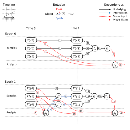
Figure 2: This figure shows a causal diagram. An ‘epoch’ is a new model fitting cycle. Covariates for a sample at the start of an epoch are modelled by $X^{\cdot}_{e}(0)$. We presume $\left\{X^{s}_{e}(0),e\geq 0\right\}$ are independent (as are $X^{a}_{\cdot}(0)$ and $X^{\ell}_{\cdot}(0)$). We start with a sample at $t=0,e=0.$ The values $X^{s}_{0}(0)$, $X^{a}_{0}(0)$ are observed and sent to analysts (arrow 1). No predictive score is present and no interventions are made based on it, so values remain the same to $t=1$ (arrows 2). $\mathbb{E}[Y_{0}]$ depends only on covariates at $t=1$, through $f_{0}$ (arrows 3). $Y_{0}$ is observed and sent to analysts (arrow 4) who decide a function $\rho_{0}$, which is retained into epoch 1 (arrow 5). We start epoch 1 with a new independent sample. At $t=0,$ we observe $X^{s}_{1}(0)$, $X^{a}_{1}(0)$ and send them to analysts (arrow 6) who compute $\rho_{0}\left(X^{s}_{1}(0),X^{a}_{1}(0)\right)$ which is used to inform interventions $g^{a}_{1}$, $g^{\ell}_{1}$ (arrow 7) to change values $X^{a}_{e}(0),X^{\ell}_{e}(0)$ to $X^{a}_{e}(1),X^{\ell}_{e}(1)$ respectively (arrows 8). $X^{s}_{e}(0)$ is not interventionable and becomes $X^{s}_{e}(1)$ (arrow 9). $\mathbb{E}[Y_{1}]$ is determined by covariates at $t=1$ (arrows 10). Analysts use the values of $X^{s}_{1}(0)$, $X^{a}_{1}(0)$ (arrows 11), and $Y_{1}$ (arrow 12) to decide a $\rho_{1}$, which is retained (arrow 13) for epoch 2. Subsequent epochs proceed similarly to epoch 1.

where $m_{\tilde{f}}(\rho|X,Y)$ denotes a metric for closeness of $\rho$ to $\tilde{f}$, given observed data $(X,Y)$. However, if interventions are in place, the improvement in equation (6), does not imply that the actual performance improves across epochs, that is:

$$\mathbb{E}_{(X_{e}^{\star},Y_{e}^{\star})}\left[m_{\tilde{f}_{e}}(\rho_{e}|X_{e}^{\star},Y_{e}^{\star})\right]\not>$$

$$\mathbb{E}_{(X_{e+1}^{\star},Y_{e+1}^{\star})}\left[m_{\tilde{f}_{e+1}}(\rho_{e+1}|X_{e+1}^{\star},Y_{e+1}^{\star})\right].$$ (7)

This is proved by counterexample: see Supplementary Section LABEL:supp_sec:models_worse. A critical consequence of this artefact is that stakeholders may decide not to update an existing score, even if an apparently better one is available.

3.2 Dynamics of repeated naive updating

Here, we analyse the dynamics of repeated naive model updating. For this purpose, we make assumptions 1-10 and assume that $\rho_{e}$ is an oracle: the ‘$\approx$’ in equation (3) is replaced by an ‘$=$’.

At epoch 0, there are no interventions, hence the risk of observing $Y=1$ is $\mathbb{E}[Y_{0}|X_{0}(0)=(x^{s},x^{a},x^{\ell})]=f(x^{s},x^{a},x^{\ell})$. The score $\rho_{0}$ is therefore defined as

$$\rho_{0}(x^{s},x^{a})=\mathbb{E}_{X^{\ell}}[f(x^{s},x^{a},X^{\ell})],$$ (8)

where $X^{\ell}$ is denoted as in assumption 2. In subsequent epochs, $\rho_{e}$ is used to modify $x^{a}$ and $x^{\ell}$ via $g^{a}$ and $g^{\ell}$, leading to the following recursive relation:

$$\rho_{0}(x^{s},x^{a}) =\mathbb{E}_{X^{\ell}}[f(x^{s},x^{a},X^{\ell})]$$

$$\rho_{e}(x^{s},x^{a}) =\mathbb{E}_{X^{\ell}}[f(x^{s},g^{a}(\rho_{e-1}(x^{s},x^{a}),x^{a}),\phantom{)]}$$

$$\phantom{=\mathbb{E}_{X^{\ell}}[f(x^{s},}g^{\ell}(\rho_{e-1}(x^{s},x^{a}),X^{\ell}))]$$

$$\triangleq h(\rho_{e-1}(x^{s},x^{a}))$$ (9)

We briefly explore the dynamics of this recursion. Let $z\in[0,1]$ be arbitrary and denote by $S$ the substitution $(x^{s},x^{a},x^{l})=\left(x^{s},g^{a}(z,x^{a}),g^{\ell}(z,X^{\ell})\right)$. Recalling definitions of $p^{s}$, $p^{a}$ from (2), we set (for $i$ across the dimensions of $(x^{a},x^{\ell})$)

$$\delta^{g^{a}}_{i} =\frac{\partial[g^{a}(z,x^{a})]_{i}}{\partial z}\hskip 20.0pt \delta^{g^{\ell}}_{i} =\frac{\partial[g^{\ell}(z,x^{\ell})]_{i}}{\partial z}$$

$$\delta^{f^{a}}_{i} =(\nabla f|_{S})_{p^{s}+i}\hskip 20.0pt \delta^{f^{\ell}}_{i} =(\nabla f|_{S})_{p^{s}+p^{a}+i}$$

recalling assumptions 9,10 to assert that these partial derivatives exist. Assumptions 9 and 10 further imply $\delta^{f^{\ell}}_{i}>0$, $\delta^{f^{a}}_{i}>0$ and $\delta^{g^{a}}_{i}<0$, $\delta^{g^{\ell}}_{i}<0$ respectively, so

$$h^{\prime}(z) =\mathbb{E}_{X^{\ell}}\left[\sum_{i}^{p^{a}}\delta^{g^{a}}_{i}\delta^{f^{a}}_{i}+\sum_{i}^{p^{\ell}}\delta^{g^{\ell}}_{i}\delta^{f^{\ell}}_{i}\right]<0$$ (10)

and thus the recursion $\rho_{e+1}=h(\rho_{e})$ has exactly one fixed point. Call this $z_{0}$, so $z_{0}=h(z_{0})$. We now note

Theorem 1.

If $h^{\prime}(z_{0})\leq-1$ then the recursion does not converge unless $\rho_{0}=z_{0}$, and will tend toward a stable oscillation between two values. If for some (possibly unbounded) interval $R$ we have $\rho_{e}\in R$ for some $e$ and for all $z\in R$, $h(z)\in R$ and

$$\sum_{i}^{p^{a}}\left(\delta_{i}^{g^{a}}\right)^{2} \leq k_{1}, \sum_{i}^{p^{\ell}}\mathbb{E}_{X^{\ell}}\left[\left(\delta_{i}^{g^{\ell}}\right)^{2}\right] \leq k_{2}$$ (11)

$$\sum_{i}^{p^{a}}\mathbb{E}_{X^{\ell}}\left[|\delta_{i}^{f^{a}}|\right]^{2} \leq k_{3}, \sum_{i}^{p^{\ell}}\mathbb{E}_{X^{\ell}}\left[\left(\delta_{i}^{f^{\ell}}\right)^{2}\right] \leq k_{4}$$ (12)

where $\sqrt{k_{1}k_{3}}+\sqrt{k_{2}k_{4}}<1$, then

$$|\rho_{e}(x^{s},x^{a})-\rho_{e+1}(x^{s},x^{a})|\to 0$$

as $n\to\infty$.

This is proved in Supplementary Appendix LABEL:supp_sec:thm1proof. Alternative conditions for convergence (‘performative stability’) are proved in Perdomo et al. [2020].

Condition (11) states that, on average, interventions make only small change to $x^{a}$ and $x^{\ell}$ in response to small changes in $\rho$. Condition (12) states that, on average, the actual risk changes little with small changes in covariates. These conditions are sufficient but not necessary. Since $h^{\prime}(z)<0$, successive estimates of $\rho_{e}$ will oscillate around their limit. In general, a requirement for general convergence of $\rho_{e}$ restricts the type of interventions which can be in place. A simple scenario in which $\rho_{e}$ cannot converge is provided in Supplementary Section LABEL:supp_sec:oscillation, and we illustrate an example showing convergence and divergence of $\rho_{e}$ in Figure 3. We produced a simple web app illustrating this problem at https://ajl-apps.shinyapps.io/universal_replacement/

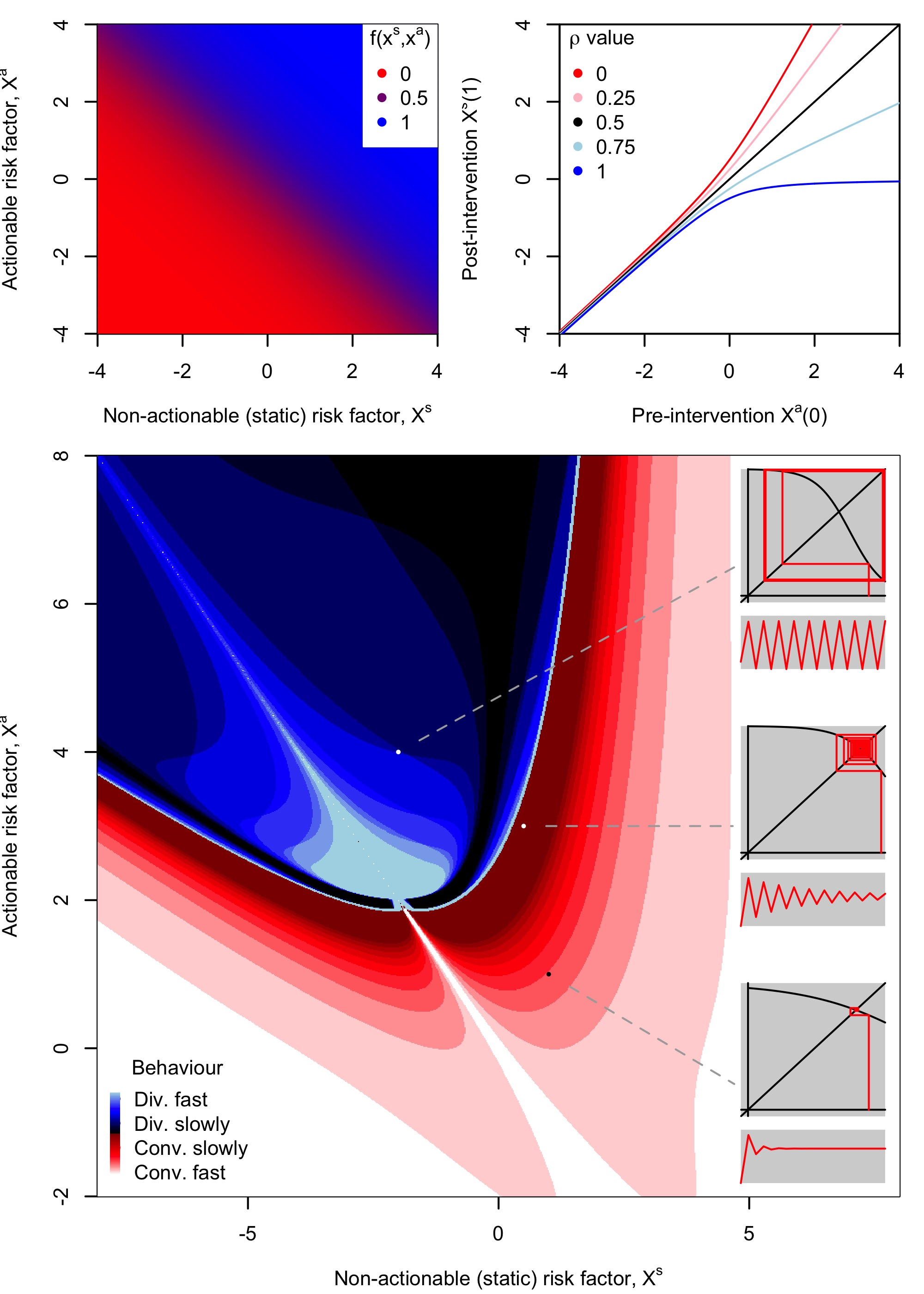
Figure 3: Example showing convergence and divergence of $\rho_{e}$ across epochs. We disregard $x^{\ell}$, $g^{\ell}$ in this example. We choose $f(x^{s},x^{a})=\textrm{logit}(x^{s},x^{a})$ (top left). We choose $g^{a}$ with the rationale that we intervene by lowering $X^{a}(0)$ when $\rho_{e}>1/2$, but allow $X^{a}(0)$ to increase when $\rho_{e}<1/2$ (that is, resources for intervention are redistributed rather than introduced), and assume that we can intervene more effectively when $X^{a}(0)$ is high ( strictly, $g^{a}(\rho,x^{a})=\frac{1}{2}\left((3-2\rho)x^{a}+(1-2\rho)\sqrt{1+(x^{a})^{2}}\right)$, top right panel). Bottom panel shows whether $\rho_{e}(x^{s},x^{a})$ converges or diverges, and how long it takes (num. epochs until $\Delta_{e}\triangleq|\rho_{e}-\rho_{e-1}|<0.01$ or $(|\Delta_{e}|>0.05\cup|\Delta_{e}-\Delta_{e-1}|<0.01)$; $|e|\leq 10$). Insets show cobweb plots for relevant recursions, and plots of $\rho_{e}$.

We may hope that naive updating, when it converges, may solve the optimisation problem in Section 2.3. It does not, and we give a specific counterexample in Supplementary Section LABEL:supp_sec:nonoptimal. Finally, we note that the dynamics above also model a related setting, where samples are tracked across epochs and interventions are permanent (Supplementary Section LABEL:supp_sec:alternative). In summary, naive updating can readily lead to wide oscillation of successive risk estimates, and even if $\rho_{e}$ does converge, the limit does not generally correspond to an optimal outcome in terms of minimising incidence of $Y$.

4 Successive adjuvancy

Note: This section and associated content (theorem 2, figures 4, 5, and associated discussions) were not included in the originally submitted version of this paper due to length. This material does not appear in the published version of this manuscript, and the reader should be aware that these sections did not undergo peer review.

We propose a second strategy for updating risk scores in which interventions are ‘built’ across successive epochs, effectively using new risk scores as adjuvants to risk scores from previous epochs, rather than replacements.

We retain assumptions 1 through 10 except assumption 2: we assume that $f_{e}$ and $\mu_{e}$ remain fixed across epochs, but $g^{a}_{e}$ and $g^{\ell}_{e}$ do not. Although we no longer consider $g^{a}_{e}$ and $g^{\ell}_{e}$ fixed across epochs, we consider fixed functions $g^{a}$ and $g^{\ell}$ which will be used as ‘building blocks’ for $g^{a}_{e}$ and $g^{\ell}_{e}$. In epoch $e$, we observe initial values $x_{e}(0)=\left(x^{a}_{e}(0),x^{s}_{e}(0),x^{\ell}_{e}(0)\right)=(x^{a}_{e},x^{s}_{e},x^{\ell}_{e})$ at $t=0$, and compute $\rho_{0}(x^{a}_{e},x^{s}_{e})$, $\rho_{1}(x^{a}_{e},x^{s}_{e})$, $\dots$, $\rho_{e-1}(x^{a}_{e},x^{s}_{e})$.

We build $g^{a}_{e}$, $g^{\ell}_{e}$ as follows. We begin by intervening on $x^{s}_{e}(0),x^{\ell}_{e}(0)$ according to $\rho_{0}$ and the building block functions $g^{a}$, $g^{\ell}$ to get $g^{a}(\rho_{0},x^{a}_{e})$, $g^{l}(\rho_{0},x^{\ell}_{e})$. We then intervene on these new values according to $\rho_{1}$, to get $g^{a}\left(\rho_{1},g^{a}(\rho_{0},x^{a}_{e})\right)$, $g^{\ell}\left(\rho_{1},g^{\ell}(\rho_{0},x^{\ell}_{e})\right)$. We then intervene on these values according to $\rho_{2}$, and so on. The intervention functions at epoch $e$ are thus defined as

$$g^{a}_{e}(\rho,x^{a}) =g^{a}\left(\rho_{e-1},g^{a}\left(\rho_{e-2},\dots,g^{a}(\rho_{0},x^{a})\dots\right)\right)$$

$$g^{\ell}_{e}(\rho,x^{\ell}) =g^{\ell}\left(\rho_{e-1},g^{\ell}\left(\rho_{e-2},\dots,g^{\ell}(\rho_{0},x^{a})\dots\right)\right)$$

taking $x^{s}$ at some fixed value, and $\rho_{0}$, $\rho_{1}$, $\dots$, $\rho_{e-1}$ as fixed functions. We also presume again that $\rho_{e}$ is an oracle; that is, that the approximation in equation 3 is perfect. This enables construction of a recursive definition:

$$g^{a}_{0}(\cdot,x^{a}) =x^{a}$$

$$g^{\ell}_{0}(\cdot,x^{\ell}) =x^{\ell}$$

$$\rho_{0}=\rho_{0}(x^{s},x^{a}) =\mathbb{E}_{X^{\ell}}[f\left(x^{s},x^{a},X^{\ell}\right)]$$

$$g^{a}_{1}(\rho_{0},x^{a}) =g^{a}(\rho_{0},x^{a})$$

$$g^{\ell}_{1}(\rho_{0},x^{\ell}) =g^{\ell}(\rho_{0},x^{\ell})$$

$$\rho_{1}=\rho_{0}(x^{s},x^{a}) =\mathbb{E}_{X^{\ell}}[f\left(x^{s},g^{a}_{1}(\rho_{0},x^{a}),g^{\ell}_{1}(\rho_{0},X^{\ell})\right)]$$

$$g^{a}_{e+1}(\rho_{e},x^{a}) =g^{a}(\rho_{e},g^{a}_{e}\left(\rho_{e-1},x^{a})\right)$$

$$g^{\ell}_{e+1}(\rho_{e},x^{\ell}) =g^{\ell}(\rho_{e},g^{\ell}_{e}\left(\rho_{e-1},x^{\ell})\right)$$

$$\rho_{e+1}=\rho_{e+1}(x^{s},x^{a}) =\mathbb{E}_{X^{\ell}}[f\left(x^{s},g^{a}_{e+1}(\rho_{e},x^{a}),g^{\ell}_{e+1}(\rho_{e},X^{\ell})\right)]$$ (14)

4.1 Dynamics of successive adjuvancy

The dynamics of this system are more complex than that of naive updating. However, under much simplified circumstances: a univariate $x^{a}$, and disregarding $x^{l}$, we show the following:

Theorem 2.

Assume the following:

1. $g^{\ell}(\cdot,x^{\ell})=g^{\ell}_{e}(\cdot,x^{\ell})=x^{\ell}$, and $X^{\ell}_{e}\sim\delta_{0}$ (so all terms involving $\ell$ can be omitted from recursion 14)

2. $x^{a}$ is univariate ($p^{a}=1$)

3. $\frac{\partial}{\partial x^{a}}f(x^{s},x^{a})>0$

4. For some unique $\rho_{eq}$ we have $\forall x\hskip 5.0ptg^{a}(\rho_{eq},x)=x$, and $\forall(x,\rho\neq\rho_{eq})\hskip 5.0ptg^{a}(\rho,x)\neq x$

For brevity we define $f(x)=f(x^{s},x)$ and denote by $S_{2}$ the substitution $(\rho,x^{a})\to(r,f^{-1}(r)$. Now if, for some interval $I$ containing $\rho_{eq}$, we have $\rho_{e}\in I$ for some $e<\infty$, and for all $r\in I$, we have

$$\left|\frac{\partial}{\partial r}f(g^{a}(r,f^{-1}(r)))\right|=\left|f^{\prime}\left(g^{a}(r,f^{-1}(r)\right)\left(\frac{\frac{\partial g^{a}}{\partial x^{a}}|_{S_{2}}}{f^{\prime}(f^{-1}(r))}+\frac{\partial g^{a}}{\partial r}|_{S_{2}}\right)\right|<1$$ (15)

then

$$\rho_{e}(x^{s},x^{a}) \to\rho_{eq}$$

$$P\left(Y_{e}|(X^{s}_{e}(0),X^{a}_{e}(0))=(x^{s},x^{a})\right) \to\rho_{eq}$$

$$g^{a}_{e}(\rho_{e-1},x^{a}) \to\{x:f(x^{s},x)=\rho_{eq}\}=f^{-1}(\rho_{eq})$$ (16)

as $e\to\infty$.

This is proved in Supplementary Section LABEL:supp_sec:thm2proof. Although limited to simplified circumstances, this results of this theorem warrant some interpretation. We may consider $\rho_{eq}$ to be an ‘equivocal risk’: that is, a risk at which the value of $x^{a}$ remains the same. The theorem roughly states that, for sufficiently slowly-changing $f$ and $g^{a}$, interventions will build towards a point in which interventions bring everyone to almost the same (equivocal) risk level.

For certain reasonable values of $f$ and $g^{a}$, including those used for figure 3, the derivative of $h_{2}$ can change sign, leading to chaotic behaviour of $\rho_{e}$ (figure 4).

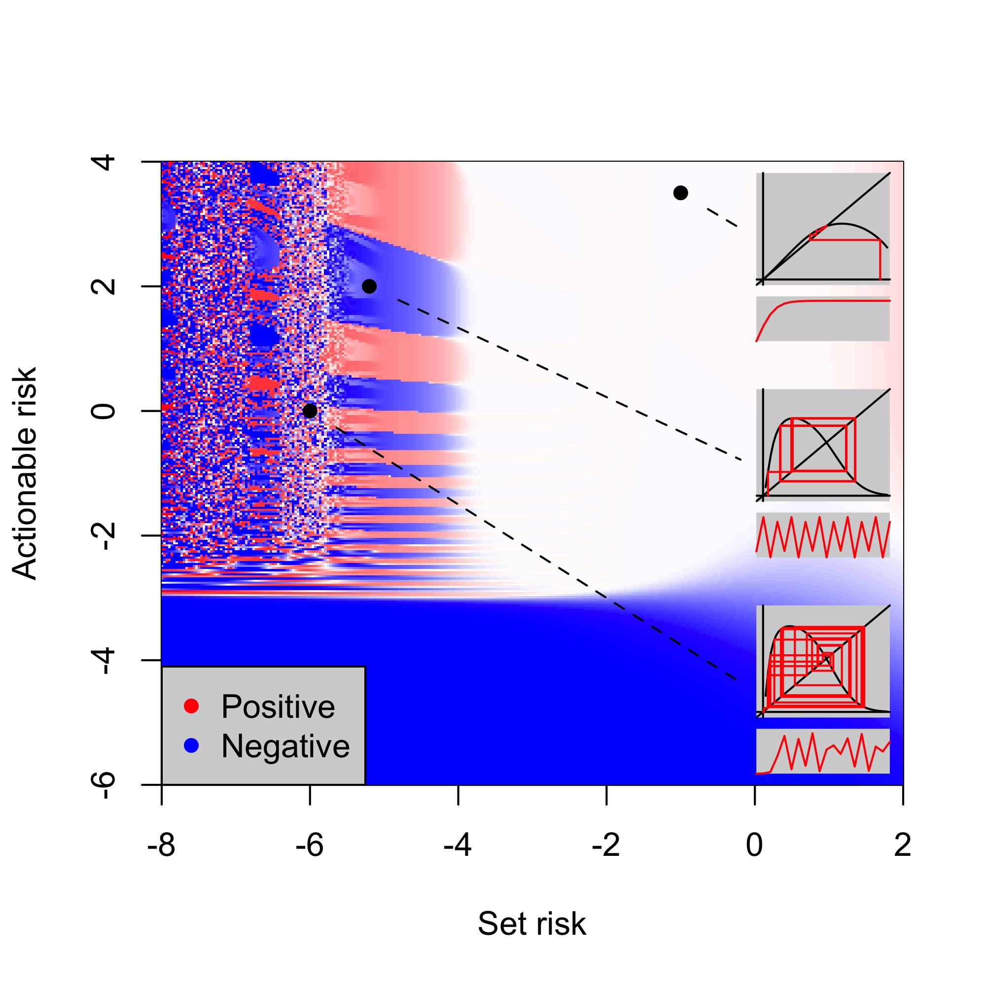
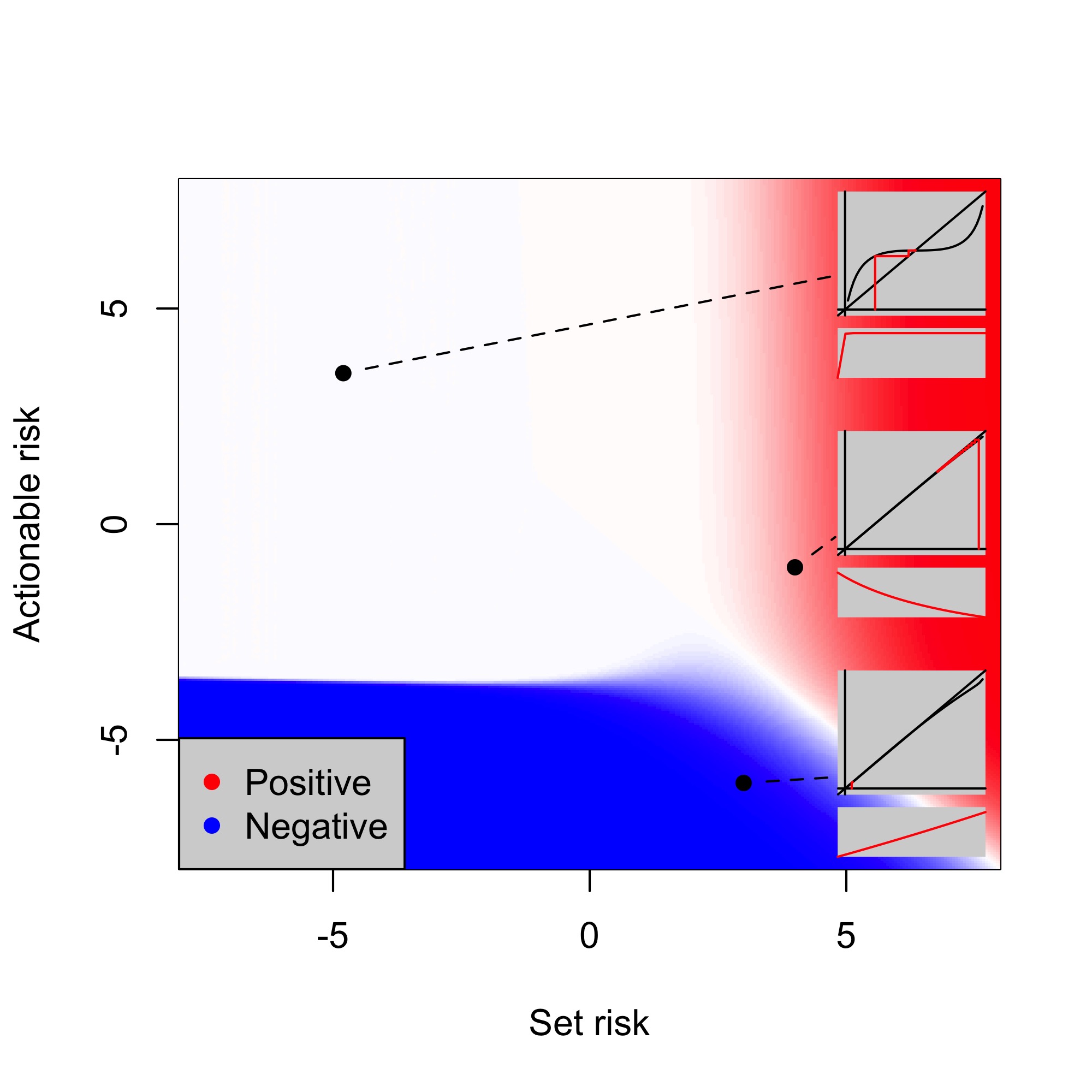
Figure 4: Dynamics of successive adjuvancy. In both panels, $f(x^{s},x^{a})=\textrm{logit}(x^{s}+x^{a})$, we have $\rho_{eq}=1/2$ and the colour indicates the difference $\rho_{e}-\rho_{eq}$ for $e=20$. The left panel shows dynamics in which $g^{a}$ has the same form as for figure 3, and can be seen to lead to chaotic behaviour of $\rho_{e}$ for some values of $(x^{s},x^{a})$. The right-hand panel uses $g^{a}(\rho,x^{a})=x^{a}-4(1-\rho)\textrm{logit}(x^{a})$, and $\rho_{e}$ can be seen to converge to $\rho_{eq}$ everywhere, albeit at different rates.

An advantage of successive adjuvancy over naive replacement is that risk scores from previous epochs $\rho_{0}$, $\rho_{1}$, $\dots$, $\rho_{e-1}$ have an immediate interpretation as unbiased estimates of risk estimates through the process of intervention. If we consider the interventions $g^{a}_{e}$, $g^{\ell}_{e}$ as a series of interventions of type $g^{a}$, $g^{\ell}$ applied in succession, then $\rho_{0}$ is the true risk ($P(Y)$) before applying $g^{a}$, $g^{\ell}$ at all, $\rho_{1}$ is the true risk after applying $g^{a}$, $g^{\ell}$ once in response to $\rho_{0}$, $\rho_{2}$ is the true risk after applying $g^{a}$, $g^{\ell}$ firstly in response to $\rho_{0}$ and subsequently in response to $\rho_{1}$, and so on. Specifically, $\rho_{e-1}$ is the risk of $Y$ immediately before applying $g^{a}$, $g^{\ell}$ for the final ($e$th) time. When used for this final time, $g^{a}$ and $g^{\ell}$ are applied in response to $\rho_{e-1}$ itself. Figure 5 illustrates this idea for epochs 0 and 1 using the format of figure 1. Seen in this way, repeatedly adjusting covariates on the basis of new risk estimates resembles a ‘boosting’ strategy, in which each new $\rho_{e}$ captures the residual risk from $\rho_{0}$ through $\rho_{e-1}$, which seems a logical approach in a real-world situation.

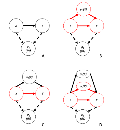
Figure 5: Underlying causality structure of successive adjuvancy. Panel A shows structure in a score-naive setting where $\rho_{0}$ is fitted. Panel B shows the causal structure when $\rho_{1}$ is fitted; as for figure 1, $\rho_{1}$ models a setting (coloured red) in which $\rho_{0}$ forms an additional causal pathway from $X$ to $Y$. Undernaive updating (panel C), $\rho_{1}$ replaces $\rho_{0}$, and is used to model a scenario distinct from that to which it was fitted. However, in successive adjuvancy (panel D), $\rho_{1}$ is an adjuvant to $\rho_{0}$, and thus still operates on the same system to which it was fitted. In panel D, $\rho_{1}$ is used to guide interventions after having intervened on $\rho_{0}$.

An implementation of successive adjuvancy is included in our web app at https://ajl-apps.shinyapps.io/universal_replacement/.

5 Strategies to avoid this problem

Naive updating is an appropriate method for updating risk scores if no interventions are being made (that is, $g^{a}(\rho,x^{a})=x^{a}$ and $g^{\ell}(\rho,x^{\ell})=x^{\ell}$), as may be the case if a risk score is used for prognosis only, rather than to guide actions. It may also be appropriate if we do not aim to solve the constrained optimisation problem in Section 2.3, and are only concerned with accuracy of the model: in that case, under at least the conditions of Theorem 1, naive updating will lead to estimates $\rho_{e}(x^{s},x^{a})$ converging as $e\to\infty$ to a setting in which $\rho_{e}$ accurately estimates its own effect: conceptually, $\rho_{e}(x^{s},x^{a})$ estimates the probability of $Y$ after interventions have been made on the basis of $\rho_{e}(x^{s},x^{a})$ itself [Perdomo et al., 2020]. Naive updating is otherwise generally not advisable, although a range of alternative modelling strategies do not lead to the same problems.

We demonstrate three general strategies for avoiding the naive updating problem below. We describe how each of these accomplishes this and compare their advantages in Supplementary section LABEL:supp_sec:solution_comparison. We describe how an implementation of each strategy may look in the context of a toy example in supplementary section LABEL:supp_sec:solution_illustration.

Successive adjvuancy may be an appropriate method for updating risk scores if eventual convergence can be proven and a progression of all samples towards the same risk level is be a desirable outcome. Such an outcome clearly does not generally solve the constrained optimisation problem in 2.3 as the cost may be arbitrarily large. Although $g^{a}_{e}$ and $g^{\ell}_{e}$ are variable, they are entirely built of successive applications of $g^{a}$ and $g^{\ell}$, which may not be practical.

5.1 More complex modelling and more data

An obvious way to avoid the problem is to model the setting completely, including the effect of any interventions. Methods of this type would include explicit causal modelling, as used in related problems [Sperrin et al., 2018], or counterfactual inference, which has been suggested as a direct approach to the problem [Sperrin et al., 2019]. These approaches would require knowledge or accurate inference of $g^{\ell}$ and $g^{a}$, or observation of covariates at several points in each epoch [Sperrin et al., 2018].

A second approach is to consider data from previous epochs alongside the current data when fitting $\rho_{e}$. Such data can be used as a prior on the fitted model [Alaa and van der Schaar, 2018] and could be used to infer model elements: $\mu_{e}$, $g^{\ell}$, $g^{a}$, and $f$. If accurate data were available, oscillatory effects could even be detected and avoided. A difficulty with this approach in a realistic setting is in distinguishing whether inaccuracies in older models are due to drift in the underlying system [Quionero-Candela et al., 2009] (in our case, $f$ and $\mu_{e}$) or due to the effects of intervention. Indeed, the problems with naive updating can be seen as treating model inaccuracies as though they are due to the first effect, when they are in fact due to the second. Definitive assertion of the cause of inaccuracies will, again, generally require more frequent observation of covariates.

5.2 Hold out set

A straightforward and potentially practical means to avoid the problems associated with naive updating is to retain a set of samples in each epoch for which $\rho_{e}$ is not calculated, and hence cannot guide intervention. For such samples, $X_{e}(0)=X_{e}(1)$, so a regression of $Y$ on $X_{e}(0)$ restricted to these ‘held out’ samples can be used as an unbiased estimate for $f_{e}$. If the hold out set is randomly selected, this would emulate a clinical trial which enables us to assess the effect of predictive scores (and their associated interventions) across epochs.

A problem with this approach is that any benefit of the risk score-guided intervention is lost for individuals in the hold-out set. Careful consideration of the ethical consequences of this strategy is therefore required.

5.3 Control interventions

A radically different option is the direct specification of the interventions $g^{\ell}_{e}$ and $g^{a}_{e}$ in each epoch, considering $\rho_{e}$, $\mu_{e}$ constant, and $f_{e}$ to change only slightly with $e$. This enables directly addressing the constrained optimisation problem in Section 2.3.

If $X^{\ell}$ can be disregarded, and we may regard $f_{e-1}$ as an unbiased estimate of $f_{e}$, then we may take a simple inductive approach:

1. At the end of epoch 0, infer $f_{0}$ and $\mu_{0}$. Given some fixed functions $\rho$, $c^{a}$, find a function $g^{a}_{1}$ which solves the constrained optimisation problem in section 2.3 assuming $f_{1}=f_{0}$, $\rho_{1}=\rho_{0}$. Implement this intervention.

2. At the end of epoch $e>0$, regress $Y_{e}$ on

   $$X_{e}(1)=\left(X^{s}_{e}(0),g^{a}_{e}\Big{(}\rho(X^{s}_{e}(0),X^{a}_{e}(0)),X^{a}_{e}(0)\Big{)}\right)$$

   to attain an unbiased estimate of $f_{e}$. Now solve the constrained optimisation problem to optimise $g^{a}_{e+1}$, assuming $f_{e+1}=f_{e}$ and $\rho_{e+1}=\rho_{e}$

Thus in each epoch an unbiased update of $f_{e}$ can be made, and the constrained optimisation problem can be directly solved. If $X^{\ell}$ is present, the problem is more complex. We suggest this general case as an open problem (see Supplementary Section LABEL:supp_sec:open).

A problem with this approach in a medical setting is that specification of $g^{a}_{e}$ may cause the procedure to be subject to medical device regulation [MHRA, 2019]. Implications of these regulatory processes map to our potential solutions; for example, countries in the EU [EU Council, 2014] have only developed regulatory processes to the point of accommodating static risk scores, and by extension currently treat updated scores as new tools. In these cases a separate evaluation exercise, such as testing on a hold-out, is necessary to demonstrate efficacy prior to dissemination, which would also remedy the problems of naive updating (although costs of repeated formal evaluations of effectiveness, and the ethics of a hold-out, may be a concern). However, the US FDA have proposed an alternative ‘total-life-cycle’ approach [USFDA et al., 2019] which allows for model updating (contingent on defining a performance monitoring mechanism), which, given the problems of naive updating, is potentially seriously flawed.

6 Formulation as control-theoretic/ reinforcement learning problem

Control theory [Bertsekas, 1995] and its modern incarnation, reinforcement learning [Sutton and Barto, 2018], study temporal problems where multiple actions are available at each time step. The aim of the field is to come up with an optimal policy either from the start or, in the partially observable case, a mechanism that quickly converges to the optimal policy. In the latter the regret is considered to be how much utility is lost compared to using the optimal policy from the start. The methods underlying this, like dynamic programming, are used in a variety of fields such as; playing go [Silver et al., 2018], in dynamic treatment strategy [Alaa and van der Schaar, 2018] and mechanical and electrical engineering. Here we use the formulation of a Partially Observable Markov Decision Processes (POMDP) [Yuksel, 2017], and adopt the notation from [Wang et al., 2019] whereby we consider the POMDP as a 7-Tuple $\left(\mathcal{S},\mathcal{A},\mathcal{T},\mathcal{R},\Omega,\mathcal{Z},\gamma\right)$:

• $\mathcal{S},\mathcal{A}$ and $\Omega$ are spaces of states, actions and observations.

• $\mathcal{T}$ is the transition kernel that describes the evolution given state and action, e.g. $s_{e+1}\sim\mathcal{T}(\cdot\mid s_{e},a_{e})$ (i.e. a set of conditional transition probabilities between states and actions).

• $\mathcal{Z}$ is a kernel for the observation given the state, e.g. $o_{e+1}\sim\mathcal{Z}(\cdot\mid s_{e},a_{e})$.

• $r_{e}$ represents our reward for being in state $s$ and taking action $a$ at time (or equivalently epoch) $e$, and is sampled from $\mathcal{R}$ - i.e. $r_{e}\sim\mathcal{R}(s_{e},a_{e})$

• $\gamma$ is a discount factor that down-weighs future rewards if $0<\gamma<1$.

A solution candidate is a policy

$$a_{e}\sim\pi\left(\left\{o_{s},r_{s},a_{s}\right\}_{s=1}^{e-1}\right)$$

which aims to maximise

$$\mathbb{E}\sum_{e=1}^{M}\gamma^{e-1}r(s_{e},a_{e})$$

where $M$ represents the maximum number of time/epoch steps. Other reward/utility parametrisations are possible e.g. to include a final pay off or infinite time horizon pay off. Several options for reward function construction are detailed in [Liu et al., 2014, Yu et al., 2019, Wirth et al., 2017]. The beauty of this framework is the flexibility: aspects such as optimisation under uncertainty can be included by including parameters of reward, transition and observation processes into the (unobserved) state variable.

We cast the above in this framework:

$$s_{e} =\left(X_{e}(0),X_{e}(1),Y_{e}\right)$$

$$a_{e} =\rho_{e}$$

$$o_{e} =\left((X_{e}^{s}(0),X_{e}^{a}(0)),Y_{e}\right)$$

$$r_{e} =\mathbb{P}\left(\bar{Y}_{e+1}\mid s_{e},a_{e}\right)$$

with $\bar{Y}$ corresponding to the rate of events in total population.

The transition kernel from $s_{e}$ to $s_{e+1}$ consists of; sampling $X_{e+1}(0)$ (note that this sampling is independent of $s_{e}$), intervening using this sample with $\rho_{e}$ to form $X_{e+1}(1)$, and then using these values to sample $Y_{e+1}$ from the resulting conditional distribution. Finally we note that given Assumption 5 our policy $a_{e}\sim\pi(o_{e},r_{e},a_{e})$ as previous epochs are ignored. Indeed, this assumption also implies that $s_{e+1},o_{e+1}$ and $r_{e}$ only depend on the previous state through $a_{e}=\rho_{e}$. In the control view point it is also easy to formulate the longitudinal problem (this corresponds to setting $X_{e+1}(0)=X_{e}(1)$).

The description above allows to use methods of the field such as Q-learning, (approximate dynamic programming), PDE-based approaches such as the Hamilton Jacobi Bellman equation and many more. These methods create a policy which maps the historical observations to an action (for the problem at hand a risk score function). Most of the rigorous methods require a low dimensional state space [Powell, 2007].

7 Discussion

In this work, we elaborate on the issue raised by Lenert and Sperrin [Lenert et al., 2019, Sperrin et al., 2019] and propose a framework for quantitatively modelling its effects, with a particular focus on a model which is updated repeatedly. We demonstrate some consequences of ignoring this problem, and note that they occur even in highly idealised circumstances. Although the problem can generally be avoided by more complex and complete modelling, we consider that this is often impractical: a full consideration of the setting in which a model will eventually be used is not generally considered until the model is to be implemented [Lipton and Steinhardt, 2018].

The formulation of the constrained optimisation problem in section 2.3 makes it clear that for fixed $g^{\ell}$, $g^{a}$, the best possible $\rho_{e}$ is not necessarily the oracle estimator in equation 3. However, many machine learning models tend to focus on accurate prediction of outcomes [Nashef et al., 2012], rather than directly solving problems of the type in section 2.3; hence, the naive updating setting considers a $\rho_{e}$ which does exactly this. In the naive updating setting, we are assuming an analyst who ignores this effect.

The model presented here is not a full description of modern predictive scoring systems; however, it is extensible in various ways (some detailed in Supplementary Section LABEL:supp_sec:open). In particular, $g^{\ell}$ and $g^{a}$ could be random-valued rather than deterministic. We also note that we assume a covariate value after intervention confers the same contribution to risk of $Y$ as it does when it takes the same value ‘naturally’, which may not be realistic.

We assume we are ‘starting over’ with new samples at the beginning of each epoch, and for naive updating, we assume that covariate values are identically distributed. The basis for this assumption is that we generally expect interventions to be zero-sum: that is, the risk score guides a redistribution of intervention rather than introduction of interventions, so the total effect on the sample population remains roughly the same in each epoch. In this assumption, we differ from that in the analysis by Lenert [2019]. We can alternatively interpret this assumption as taking all interventions as being short-term and having ‘worn off’ by the start of the next epoch. The problem raised here also exists for the more general setting when interventions have long term effects and we consider longitudinal effects.

An important consideration in model updating is ‘stability’ of successive predictions: in our setting, whether successive values of $\rho_{e}$ converge. Colloquially, we can take ’stability’ to mean that if the underlying system being modelled does not change, then updating a model will leave it unchanged; the model predicts its own effect. General conditions for stability are considered in Perdomo et al. [2020] , who differentiate between stability in which $\rho$ optimises a loss given its own effect, and ‘performative optimality’, in which $\rho$ globally optimises a loss. Although we highlight that stability does not generally guarantee that the model is getting the best outcome (according to the constrained optimisation problem in section 2.3), we note that stability has real-world advantages: in particular, trust in a model will generally be better if it appears to be stable.

In the setting where models change at each epoch, if $m_{\tilde{f}_{e}}$ is known at the current epoch $e$, we note a fair comparison of models is one which compares models built using the training data available at the current epoch. If $m_{\tilde{f}_{e}}$ is not known, then a holdout set for test data must be used so a fair comparison can be made using an estimate of $m_{\tilde{f}_{0}}$ (assuming $\tilde{f}_{0}\approx f$). This is because at epoch $e$ we only have access to $(X_{e}(0),Y_{e})$ and not $X_{e}(1)$, and so we are not able to properly gain insight to the behaviour of $\tilde{f}_{e}$ needed to provide an estimate of $m_{\tilde{f}_{e}}$. An attempt to estimate $m_{\tilde{f}_{e}}$ using $(X_{e}(0),Y_{e})$ implicitly assumes that $Y_{e}$ directly depends on $X_{e}(0)$, and as a result $\rho_{e}$ would appear much closer to $\tilde{f}_{e}$ than is the case. Put simply, by implementing naive model updating not only may performance severely worsen (even if better models were used), but in not providing a holdout test set stakeholders may not even be able to recognise that performance is worsening as the number of epochs increase.

In essence, we provide a causal framework within which to understand a crucial issue in regulation of machine learning and AI-based tools in health and further afield, demonstrating that approaches which incorporate naive updating are unlikely to be fit for purpose. Moreover, even where solutions are available to address the bias introduced by updating on ‘real-world’ data in which outcomes represent (at least in part) the effects of an algorithm, these restrict the potential of ‘online’ and frequently updated solutions. We hope that our work will foster discussion of this interesting problem, which is becoming increasingly pertinent as machine-learning based predictive scores become widely used to guide decision making, and policymakers act to address how to regulate these tools to ensure safety and effectiveness.

Code availability

Code to reproduce relevant plots and examples is available at github.com/jamesliley/model_updating.

Acknowledgements

We thank the Alan Turing Institute, MRC Human Genetics Unit at the University of Edinburgh, Durham University, University of Warwick, Wellcome Trust, Health Data Research UK, and Kings College Hospital, London for their support of the authors. This problem was first identified in our circumstance by LJMA. We thank Dr Ioanna Manolopoulou for helping to draw our attention to the imminence of this problem.

JL, CAV and LJMA were partially supported by Wave 1 of The UKRI Strategic Priorities Fund under the EPSRC Grant EP/T001569/1, particularly the “Health” theme within that grant and The Alan Turing Institute; JL, BAM, CAV, LJMA and SJV were partially supported by Health Data Research UK, an initiative funded by UK Research and Innovation, Department of Health and Social Care (England), the devolved administrations, and leading medical research charities; SRE is funded by the EPSRC doctoral training partnership (DTP) at Durham University, grant reference EP/R513039/1; LJMA was partially supported by a Health Programme Fellowship at The Alan Turing Institute; CAV was supported by a Chancellor’s Fellowship provided by the University of Edinburgh.

Bibliography

- Alaa and van der Schaar [2018] A. M. Alaa and M. van der Schaar. Autoprognosis: Automated clinical prognostic modeling via bayesian optimization with structured kernel learning. arXiv preprint arXiv:1802.07207, 2018.
- Bertsekas [1995] D. P. Bertsekas. Dynamic programming and optimal control, volume 1. Athena scientific Belmont, MA, 1995.
- Elzayn et al. [2019] H. Elzayn, S. Jabbari, C. Jung, M. Kearns, S. Neel, A. Roth, and Z. Schutzman. Fair algorithms for learning in allocation problems. In Proceedings of the Conference on Fairness, Accountability, and Transparency, pages 170–179, 2019.
- EU Council [2014] EU Council. EU regulation no 2017/745 on medical devices, 2014. https://eur-lex.europa.eu/legal-content/EN/TXT/PDF/?uri=CELEX:32017R0745.
- Friedman et al. [2001] J. Friedman, T. Hastie, and R. Tibshirani. The Elements of Statistical Learning, volume 1. Springer Series in Statistics New York, 2001.
- Hyland et al. [2020] S. L. Hyland, M. Faltys, M. Hüser, X. Lyu, T. Gumbsch, C. Esteban, C. Bock, M. Horn, M. Moor, B. Rieck, et al. Early prediction of circulatory failure in the intensive care unit using machine learning. Nature Medicine, 26(3):364–373, 2020.
- Lenert et al. [2019] M. C. Lenert, M. E. Matheny, and C. G. Walsh. Prognostic models will be victims of their own success, unless…. Journal of the American Medical Informatics Association, 26(12):1645–1650, 2019.
- Lipton and Steinhardt [2018] Z. C. Lipton and J. Steinhardt. Troubling trends in machine learning scholarship. arXiv preprint arXiv:1807.03341, 2018.
- Liu et al. [2014] C. Liu, X. Xu, and D. Hu. Multiobjective reinforcement learning: A comprehensive overview. IEEE Transactions on Systems, Man, and Cybernetics: Systems, 45(3):385–398, 2014.
- Liu et al. [2018] L. T. Liu, S. Dean, E. Rolf, M. Simchowitz, and M. Hardt. Delayed impact of fair machine learning. In International Conference on Machine Learning, pages 3150–3158. PMLR, 2018.
- MHRA [2019] MHRA. Medical device stand-alone software including apps (including IVDMDs), 2019.
- Nashef et al. [2012] S. A. Nashef, F. Roques, L. D. Sharples, J. Nilsson, C. Smith, A. R. Goldstone, and U. Lockowandt. Euroscore ii. European Journal of Cardio-Thoracic Surgery, 41(4):734–745, 2012.
- Perdomo et al. [2020] J. Perdomo, T. Zrnic, C. Mendler-Dünner, and M. Hardt. Performative prediction. In International Conference on Machine Learning, pages 7599–7609. PMLR, 2020.
- Powell [2007] W. B. Powell. Approximate Dynamic Programming: Solving the Curses of Dimensionality. John Wiley & Sons, Oct. 2007.
- Quionero-Candela et al. [2009] J. Quionero-Candela, M. Sugiyama, A. Schwaighofer, and N. D. Lawrence. Dataset Shift in Machine Learning. The MIT Press, 2009.
- Rahimian et al. [2018] F. Rahimian, G. Salimi-Khorshidi, A. H. Payberah, J. Tran, R. A. Solares, F. Raimondi, M. Nazarzadeh, D. Canoy, and K. Rahimi. Predicting the risk of emergency admission with machine learning: Development and validation using linked electronic health records. PLoS Medicine, 15(11):e1002695, 2018.
- Shi et al. [2020] Z. R. Shi, Z. S. Wu, R. Ghani, and F. Fang. Bandit data-driven optimization: Ai for social good and beyond. arXiv preprint arXiv:2008.11707, 2020.
- Silver et al. [2018] D. Silver, T. Hubert, J. Schrittwieser, I. Antonoglou, M. Lai, A. Guez, M. Lanctot, L. Sifre, D. Kumaran, T. Graepel, et al. A general reinforcement learning algorithm that masters chess, shogi, and go through self-play. Science, 362(6419):1140–1144, 2018.
- Sperrin et al. [2018] M. Sperrin, G. P. Martin, A. Pate, T. Van Staa, N. Peek, and I. Buchan. Using marginal structural models to adjust for treatment drop-in when developing clinical prediction models. Statistics in Medicine, 37(28):4142–4154, 2018.
- Sperrin et al. [2019] M. Sperrin, D. Jenkins, G. P. Martin, and N. Peek. Explicit causal reasoning is needed to prevent prognostic models being victims of their own success. Journal of the American Medical Informatics Association, 26(12):1675–1676, 2019.
- Sutton and Barto [2018] R. S. Sutton and A. G. Barto. Reinforcement Learning, second edition: An Introduction. MIT Press, Nov. 2018.
- USFDA et al. [2019] USFDA et al. Proposed regulatory framework for modifications to artificial intelligence/machine learning (AI/ML)-based software as a medical device (samd)-discussion paper, 2019. https://www.fda.gov/files/medical\%20devices/published/US-FDA-Artificial-Intelligence-and-Machine-Learning-Discussion-Paper.pdf.
- Wallace et al. [2014] E. Wallace, E. Stuart, N. Vaughan, K. Bennett, T. Fahey, and S. M. Smith. Risk prediction models to predict emergency hospital admission in community-dwelling adults: a systematic review. Medical Care, 52(8):751, 2014.
- Wang et al. [2019] Y. Wang, B. Liu, J. Wu, Y. Zhu, S. S. Du, L. Fei-Fei, and J. B. Tenenbaum. DualSMC: Tunneling differentiable filtering and planning under continuous POMDPs. ijcai.org, 2019.
- Wirth et al. [2017] C. Wirth, R. Akrour, G. Neumann, J. Fürnkranz, et al. A survey of preference-based reinforcement learning methods. Journal of Machine Learning Research, 18(136):1–46, 2017.
- Yu et al. [2019] C. Yu, J. Liu, and S. Nemati. Reinforcement learning in healthcare: A survey. arXiv preprint arXiv:1908.08796, 2019.
- Yuksel [2017] S. Yuksel. Control of stochastic systems. Queen’s University Mathematics and Engineering and Mathematics and Statistics, 2017. https://mast.queensu.ca/~math472/Math472872LectureNotes.pdf.