Calibrated Language Model Fine-Tuning for In- and Out-of-Distribution Data

Abstract

Fine-tuned pre-trained language models can suffer from severe miscalibration for both in-distribution and out-of-distribution (OOD) data due to over-parameterization. To mitigate this issue, we propose a regularized fine-tuning method. Our method introduces two types of regularization for better calibration: (1) On-manifold regularization, which generates pseudo on-manifold samples through interpolation within the data manifold. Augmented training with these pseudo samples imposes a smoothness regularization to improve in-distribution calibration. (2) Off-manifold regularization, which encourages the model to output uniform distributions for pseudo off-manifold samples to address the over-confidence issue for OOD data. Our experiments demonstrate that the proposed method outperforms existing calibration methods for text classification in terms of expectation calibration error, misclassification detection, and OOD detection on six datasets. Our code can be found at https://github.com/Lingkai-Kong/Calibrated-BERT-Fine-Tuning.

1 Introduction

Pre-trained language models have recently brought the natural language processing (NLP) community into the transfer learning era. The transfer learning framework consists of two stages, where we first pre-train a large-scale language model, (e.g., BERT (Devlin et al., 2019), RoBERTa (Liu et al., 2019), ALBERT (Lan et al., 2020) and T5 (Raffel et al., 2019)) on a large text corpus and then fine-tune it on downstream tasks. Such a fine-tuning approach has achieved SOTA performance in many NLP benchmarks (Wang et al., 2018, 2019).

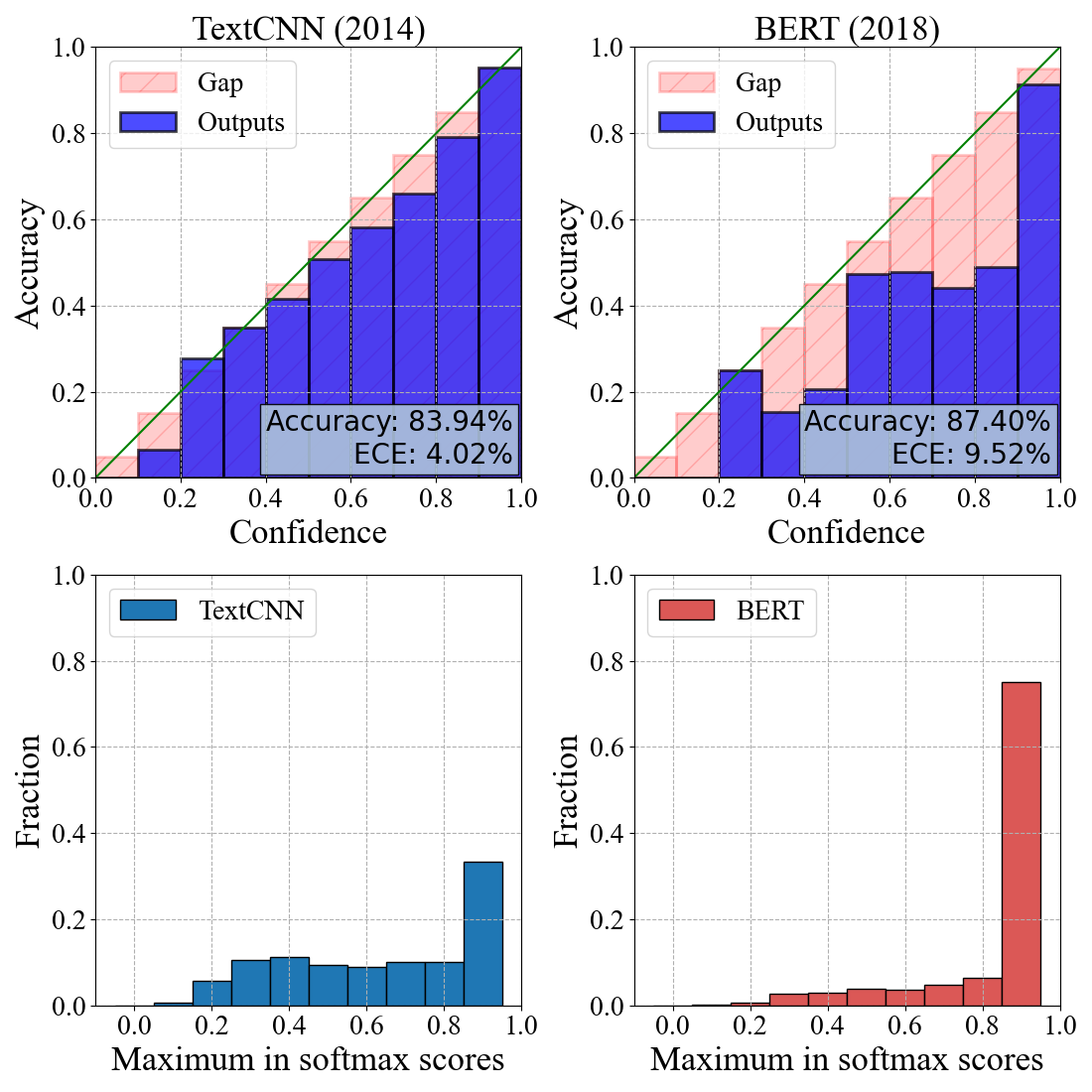
Figure 1: The reliability diagrams on in-distribution data (the first row) and the histograms of the model confidence on out-of-distribution (OOD) data (the second row) of CNN (Kim, 2014) and fine-tuned BERT-MLP classifier (Devlin et al., 2019). Though BERT improves classification accuracy, it makes over-confident predictions for both in-distribution and OOD data.

Many applications, however, require trustworthy predictions that need to be not only accurate but also well calibrated. In particular, a well-calibrated model should produce reliable confident estimates for both in-distribution and out-of-distribution (OOD) data: (1) For in-distribution data, a model should produce predictive probabilities close to the true likelihood for each class, i.e., confidence $\approx$ true likelihood. (2) For OOD data, which do not belong to any class of the training data, the model output should produce high uncertainty to say ‘I don’t know’, i.e., confidence $\approx$ random guess, instead of producing absurdly wrong yet wildly confident predictions. Providing such calibrated output probabilities can help us to achieve better model robustness (Lee et al., 2018), model fairness (Chouldechova, 2017) and improve label efficiency via uncertainty driven learning (Gal et al., 2017; Siddhant and Lipton, 2018; Shen et al., 2018).

Unfortunately, Guo et al. (2017) have shown that due to over-parameterization, deep convolutional neural networks are often miscalibrated. Our experimental investigation further corroborates that fine-tuned language models can suffer from miscalibration even more for NLP tasks. As shown in Figure 1, we present the calibration of a BERT-MLP model for a text classification task on the 20NG dataset. Specifically, we train a TextCNN (Kim, 2014) and a BERT-MLP using 20NG₁₅ (the first 15 categories of 20NG) and then evaluate them on both in-distribution and OOD data. The first row plots their reliability diagrams (Niculescu-Mizil and Caruana, 2005) on the test set of 20NG₁₅. Though BERT improves the classification accuracy from $83.9\%$ to $87.4\%$, it also increases the expected calibration error (ECE, see more details in Section 2) from $4.0\%$ to $9.5\%$. This indicates that BERT-MLP is much more miscalibrated for in-distribution data. The second row plots the histograms of the model confidence, i.e., the maximum output probability, on the test set of 20NG₅ (the unseen 5 categories of 20NG). While it is desirable to produce low probabilities for these unseen classes, BERT-MLP produces wrong yet over-confident predictions for such OOD data.

Such an aggravation of miscalibration is due to the even more significant over-parameterization of these language models. At the pre-training stage, they are trained on a huge amount of unlabeled data in an unsupervised manner, e.g., T5 is pre-trained on 745 GB text. To capture rich semantic and syntactic information from such a large corpus, the language models are designed to have enormous capacity, e.g., T5 has about 11 billion parameters. At the fine-tuning stage, however, only limited labeled data are available in the downstream tasks. With the extremely high capacity, these models can easily overfit training data likelihood and be over-confident in their predictions.

To fight against miscalibration, a natural option is to apply a calibration method such as temperature scaling (Guo et al., 2017) in a post-processing step. However, temperature scaling only learns a single parameter to rescale all the logits, which is not flexible and insufficient. Moreover, it cannot improve out-of-distribution calibration. A second option is to mitigate miscalibration during training using regularization. For example, Pereyra et al. (2017) propose an entropy regularizer to prevent over-confidence, but it can needlessly hurt legitimate high confident predictions. A third option is to use Bayesian neural networks (Blundell et al., 2015; Louizos and Welling, 2017), which treat model parameters as probability distributions to represent model uncertainty explicitly. However, these Bayesian approaches are often prohibitive, as the priors of the model parameters are difficult to specify, and exact inference is intractable, which can also lead to unreliable uncertainty estimates.

We propose a regularization approach to addressing miscalibration for fine-tuning pre-trained language models from a data augmentation perspective. We propose two new regularizers using pseudo samples both on and off the data manifold to mitigate data scarcity and prevent over-confident predictions. Specifically, our method imposes two types of regularization for better calibration during fine-tuning: (1) On-manifold regularization: We first generate on-manifold samples by interpolating the training data and their corresponding labels along the direction learned from hidden feature space; training over such augmented on-manifold data introduces a smoothness constraint within the data manifold to improve the model calibration for in-distribution data. (2) Off-manifold regularization: We generate off-manifold samples by adding relatively large perturbations along the directions that point outward the data manifold; we penalize the negative entropy of the output distribution for such off-manifold samples to address the over-confidence issue for OOD data.

We evaluate our proposed model calibration method on six text classification datasets. For in-distribution data, we measure ECE and the performance of misclassification detection. For out-of-distribution data, we measure the performance of OOD detection. Our experiments show that our method outperforms existing state-of-the-art methods in both settings, and meanwhile maintains competitive classification accuracy.

We summarize our contribution as follows: (1) We propose a general calibration framework, which can be applied to pre-trained language model fine-tuning, as well as other deep neural network-based prediction problems. (2) The proposed method adopts on- and off-manifold regularization from a data augmentation perspective to improve calibration for both in-distribution and OOD data. (3) We conduct comprehensive experiments showing that our method outperforms existing calibration methods in terms of ECE, miscalssification detection and OOD detection on six text classification datasets.

2 Preliminaries

We describe model calibration for both in-distribution and out-of-distribution data.

Calibration for In-distribution Data: For in-distribution data, a well-calibrated model is expected to output prediction confidence comparable to its classification accuracy. For example, given 100 data points with their prediction confidence $0.6$, we expect $60$ of them to be correctly classified. More precisely, for a data point $X$, we denote by $Y(X)$ the ground truth label, ${\widehat{Y}}(X)$ the label predicted by the model, and $\widehat{P}(X)$ the output probability associated with the predicted label. The calibration error of the predictive model for a given confidence $p\in(0,1)$ is defined as:

$$\mathcal{E}_{p}=|\mathbb{P}(\widehat{Y}(X)=Y(X)|\widehat{P}(X)=p)-p|.$$ (1)

As (1) involves population quantities, we usually adopt empirical approximations (Guo et al., 2017) to estimate the calibration error. Specifically, we partition all data points into $M$ bins of equal size according to their prediction confidences. Let $\mathcal{B}_{m}$ denote the bin with prediction confidences bounded between $\ell_{m}$ and $u_{m}$. Then, for any $p\in[\ell_{m},u_{m})$, we define the empirical calibration error as:

$$\widehat{\mathcal{E}}_{p}=\widehat{\mathcal{E}}_{m}=\frac{1}{|\mathcal{B}_{m}|}\Big{|}\sum_{i\in\mathcal{B}_{m}}\big{[}\mathbf{1}(\widehat{y}_{i}=y_{i})-\widehat{p}_{i}\big{]}\Big{|},$$ (2)

where $y_{i}$, $\widehat{y}_{i}$ and $\widehat{p}_{i}$ are the true label, predicted label and confidence for sample $i$.

To evaluate the overall calibration error of the predictive model, we can futher take a weighted average of the calibration errors of all bins, which is also known as the expected calibration error (ECE) (Naeini et al., 2015) defined as:

$${\rm ECE}=\sum_{m=1}^{M}\frac{|\mathcal{B}_{m}|}{n}\widehat{\mathcal{E}}_{m},$$ (3)

where $n$ is the sample size.

We remark that the goal of calibration is to minimize the calibration error without significantly sacrificing prediction accuracy. Otherwise, a random guess classifier can achieve zero calibration error.

Calibration for Out-of-distribution Data: In real applications, a model can encounter test data that significantly differ from the training data. For example, they come from other unseen classes, or they are potential outliers. A well-calibrated model is expected to produce an output with high uncertainty for such out-of-distribution (OOD) data, formally,

$$P(Y=j)=1/K\quad\forall j=1,...,K,$$

where $K$ is the number of classes of the training data. As such, we can detect OOD data by setting up an uncertainty threshold.

3 Calibrated Fine-Tuning via Manifold Smoothing

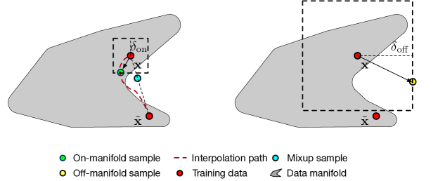
Figure 2: The on-manifold and off-manifold samples generated by our calibration procedure. Mixup adopts a coarse linear interpolation and the generated data point may deviate from the data manifold.

We consider $N$ data points of the target task $S=\{(\mathbf{x}_{i},y_{i})\}_{i=1}^{N}$, where $\mathbf{x}_{i}$’s denote the input embedding of the sentence and $y_{i}$’s are the associated one-hot labels. Let $f(\cdot)$ denote the feature extraction layers (e.g., BERT); let $g(\cdot)$ denote the task-specific layer; and let $\theta$ denote all parameters of $f$ and $g$. We propose to optimize the following objective at the fine-tuning stage:

$$\min_{\theta}\mathcal{F}(\theta)=~{}\mathbb{E}_{\mathbf{x},y\sim S}\ell(g\circ f(\mathbf{x}),y)+\lambda_{\rm on}\mathcal{R}_{\rm on}(g\circ f)+\lambda_{\rm off}\mathcal{R}_{\rm off}(g\circ f),$$ (4)

where $\ell$ is the cross entropy loss, and $\lambda_{\rm on},\lambda_{\rm off}$ are two hyper-parameters. The regularizers $\mathcal{R}_{\rm on}$ and $\mathcal{R}_{\rm off}$ are for on- and off-manifold calibration, respectively.

3.1 On-manifold Regularization

The on-manifold regularizer $\mathcal{R}_{\rm on}$ exploits the interpolation of training data within the data manifold to improve the in-distribution calibration. Specifically, given two training samples $(\mathbf{x},y)$ and $(\widetilde{\mathbf{x}},\widetilde{y})$ and the feature extraction layers $f$, we generate an on-manifold pseudo sample $(\mathbf{x}^{\prime},y^{\prime})$ as follows:

$$\mathbf{x}^{\prime*} =\mathop{\mathrm{argmin}}_{\mathbf{x}^{\prime}\in\mathbb{B}(\mathbf{x},\delta_{\rm on})}D_{x}(f(\mathbf{x}^{\prime}),f(\widetilde{\mathbf{x}})),$$ (5)

$$y^{\prime} =(1-\delta_{y})y+\delta_{y}\widetilde{y},$$ (6)

where $\delta_{\rm on}$ and $\delta_{y}$ are small interpolation parameters for data and label, and $D_{x}$ is a proper distance for features extracted by $f$ such as cosine distance, i.e., $D_{x}(\mathbf{a},\mathbf{b})=\langle\mathbf{a}/\|\mathbf{a}\|_{2},\mathbf{b}/\|\mathbf{b}\|_{2}\rangle$, and $\mathbb{B}(\mathbf{x},\delta_{\rm on})$ denotes an $\ell_{\infty}$ ball centered at $\mathbf{x}$ with a radius $\delta_{\rm on}$, i.e.,

$$\mathbb{B}(\mathbf{x},\delta_{\rm on})=\{\mathbf{x}^{\prime}~{}|~{}\|\mathbf{x}^{\prime}-\mathbf{x}\|_{\infty}\leq\delta_{\rm on}\}.$$

As can be seen, $\mathbf{x}^{\prime*}$ is essentially interpolating between $\mathbf{x}$ and $\widetilde{\mathbf{x}}$ on the data manifold, and $D_{x}(f(\cdot),f(\cdot))$ can be viewed as a metric over such a manifold. However, as $f(\cdot)$ is learnt from finite training data, it can recover the actual data manifold only up to a certain statistical error. Therefore, we constrain $\mathbf{x}^{\prime*}$ to stay in a small neighborhood of $\mathbf{x}$, which ensures $\mathbf{x}^{\prime*}$ to stay close to the actual data manifold.

This is different from existing interpolation methods such as Mixup (Zhang et al., 2018; Verma et al., 2019). These methods adopt coarse linear interpolations either in the input space or latent feature space, and the generated data may significantly deviate from the data manifold.

Note that our method not only interpolates $\mathbf{x}$ but also $y$. This can yield a soft label for $\mathbf{x}^{\prime*}$, when $\mathbf{x}$ and $\widetilde{\mathbf{x}}$ belong to different classes. Such an interpolation is analogous to semi-supervised learning, where soft pseudo labels are generated for the unlabelled data. These soft-labelled data essentially induce a smoothing effect, and prevent the model from making overconfident predictions toward one single class.

We remark that our method is more adaptive than the label smoothing method (Müller et al., 2019). As each interpolated data point involves at most two classes, it is unnecessary to distribute probability mass to other classes in the soft label. In contrast, label smoothing is more rigid and enforces all classes to have equally nonzero probability mass in the soft label.

We then define the on-manifold regularizer as

$$\mathcal{R}_{\rm on}(g\circ f)=\mathbb{E}_{(\mathbf{x}^{\prime},y^{\prime})\sim S_{\rm on}}D_{\rm KL}(y^{\prime},g\circ f(\mathbf{x}^{\prime})),$$

where $S_{\rm on}$ denotes the set of all pseudo labelled data generated by our interpolation method, and $D_{\rm KL}$ denotes the KL-divergence between two probability simplices.

Algorithm 1 Our Proposed Efficient Stochastic Optimization Algorithm for Solving (4). $d$ is the dimension of features.

for $\#$ training iterations do

     Sample a mini-batch $B=\{\mathbf{x}_{i},y_{i}\}$ from $S$.

     // Generate on-manifold samples:

     For each $\mathbf{x}_{i}\in B$, randomly select $\{\widetilde{\mathbf{x}}_{i},\widetilde{y}_{i}\}$ from $B$, initialize $\mathbf{x}^{\prime}_{i}\leftarrow\mathbf{x}_{i}+v_{i}$ with $v_{i}\sim\textrm{UNIF}[-\delta_{\rm on},\delta_{\rm on}]^{d}$

     $\Delta^{\prime}_{i}\leftarrow{\rm sign}(\nabla_{\mathbf{x}^{\prime}_{i}}D_{x}(f(\mathbf{x}_{i}^{\prime}),f(\widetilde{\mathbf{x}}_{i})))$

     $\mathbf{x}_{i}^{\prime}\leftarrow\Pi_{\|\mathbf{x}^{\prime}_{i}-\mathbf{x}_{i}\|_{\infty}\leq\delta_{\rm on}}(\mathbf{x}^{\prime}_{i}-\delta_{\rm on}\Delta^{\prime}_{i})$

     $y^{\prime}\leftarrow(1-\delta_{y})y_{i}+\delta_{y}\widetilde{y}_{i}$

     // Generate off-manifold samples:

     For each $\mathbf{x}_{i}\in B$, initialize $\mathbf{x}^{\prime\prime}_{i}\leftarrow\mathbf{x}_{i}+v^{\prime}_{i}$ with $v^{\prime}_{i}\sim\textrm{UNIF}[-\delta_{\rm off},\delta_{\rm off}]^{d}$

     $\Delta^{\prime\prime}_{i}\leftarrow{\rm sign}(\nabla_{\mathbf{x}^{\prime\prime}_{i}}\ell(g\circ f(\mathbf{x}_{i}^{\prime\prime}),y)$

     $\mathbf{x}_{i}^{\prime\prime}\leftarrow\Pi_{\|\mathbf{x}^{\prime\prime}_{i}-\mathbf{x}_{i}\|_{\infty}=\delta_{\rm off}}(\mathbf{x}^{\prime\prime}_{i}+\delta_{\rm off}\Delta^{\prime\prime}_{i})$

     Update $\theta$ using ADAM

end for

3.2 Off-manifold Regularization

The off-manifold regularizer, $\mathcal{R}_{2}$, encourages the model to yield low confidence outputs for samples outside the data manifold, and thus mitigates the over-confidence issue for out-of-distribution (OOD) data. Specifically, given a training sample $(\mathbf{x},y)$, we generate an off-manifold pseudo sample $\mathbf{x}^{{}^{\prime\prime}\ast}$ by:

$$\mathbf{x}^{{}^{\prime\prime}\ast}=\max_{\mathbf{x}^{\prime\prime}\in\mathbb{S}(\mathbf{x},\delta_{\rm off})}\!\!\!\!\ell(g\circ f(\mathbf{x}^{\prime\prime}),y),$$ (7)

where $\mathbb{S}(\mathbf{x},\delta_{\rm off})$ denotes an $\ell_{\infty}$ sphere centered at $\mathbf{x}$ with a radius $\delta_{\rm off}$.

Since we expect $\mathbf{x}^{\prime\prime\ast}$ to mimic OOD data, we first need to choose a relatively large $\delta_{\rm off}$ such that the sphere $\mathbb{S}(\mathbf{x},\delta_{\rm off})$ can reach outside the data manifold. Then, we generate the pseudo off-manifold sample from the sphere along the adversarial direction. Existing literature (Stutz et al., 2019; Gilmer et al., 2018) has shown that such an adversarial direction points outward the data manifold.

By penalizing the prediction confidence for these off-manifold samples, we are able to encourage low prediction confidence for OOD data. Hence, we define the off-manifold regularizer as

$$\mathcal{R}_{\rm off}(g\circ f)=\mathbb{E}_{\mathbf{x}^{{}^{\prime\prime}}\sim S_{\rm off}}\!\!-\mathcal{H}(g\circ f(\mathbf{x}^{\prime\prime})),$$ (8)

where $S_{\rm off}$ denotes the set of all generated off-manifold samples, and $\mathcal{H}(\cdot)$ denotes the entropy of the probability simplex.

3.3 Model Training

We can adopt stochastic gradient-type algorithms such as ADAM (Kingma and Ba, 2014) to optimize (4). At each iteration, we need to first solve two inner optimization problems in (5) and (7), and then plug $\mathbf{x}^{\prime}$ and $\mathbf{x}^{\prime\prime}$ into (4) to compute the stochastic gradient. The two inner problems can be solved using the projected sign gradient update for multiple steps. In practice, we observe that one single update step with random initialization is already sufficient to efficiently optimize $\theta$. Such a phenomenon has also been observed in existing literature on adversarial training (Wong et al., 2019). We summarize the overall training procedure in Algorithm 1.

4 Experiments

To evaluate calibration performance for in-distribution data, we measure the expected calibration error (ECE) and the misclassification detection score. For out-of-distribution data, we measure the OOD detection score.

We detect the misclassified and OOD samples by model confidence, which is the output probability associated with the predicted label $\widehat{P}(X)$. Specifically, we setup a confidence threshold $\tau\in[0,1]$, and take the samples with confidence below the threshold, i.e., $\widehat{P}(X)<\tau$, as the misclassified or OOD samples. We can compute the detection $F_{1}$ score for every $\tau$: $F_{1}(\tau)$, and obtain a calibration curve ($F_{1}(\tau)$ vs. $\tau$). Then, we set $\tau_{\rm upper}$ as the upper bound of the confidence threshold, since a well calibrated model should provide probabilities that reflect the true likelihood and it is not reasonable to use a large $\tau$ to detect them. We use the empirical Normalized Bounded Area Under the Calibration Curve (NBAUCC) as the overall detection score:

$${\rm NBAUCC}_{\tau_{\rm upper}}=\frac{1}{M}\sum_{i=1}^{M}F_{1}\large\left(\frac{\tau_{\rm upper}}{M}i\large\right),$$

where $M$ is the number of sub-intervals for the numerical integration. We set $M=50$ throughout the following experiments. Note that the traditional binary classification metrics, e.g., AUROC and AUPR, cannot measure the true calibration because the model can still achieve high scores even though it has high confidences for the misclassified and OOD samples. We provide more explanations of the metrics in Appendix C. We report the performance when $\tau_{\rm upper}=0.5$ here and the results when $\tau_{\rm upper}=0.7$ and $1$ in Appendix D.

4.1 Datasets

For each dataset, we construct an in-distribution training set, an in-distribution testing set, and an OOD testing set. Specifically, we use the following datasets:

20NG. The 20 Newsgroups dataset (20NG) contains news articles with 20 categories. We use Stanford Sentiment Treebank (SST-2) (Socher et al., 2012) as the OOD data.

20NG₁₅. We take the first 15 categories of 20NG as the in-distribution data and the other 5 categories (20NG₅) as the OOD data.

WOS (Kowsari et al., 2017). Web of Science (WOS) dataset contains scientific articles with 134 categories. We use AGnews (Zhang et al., 2015) as the OOD data.

WOS₁₀₀. We use the first 100 classes of WOS as the in-distribution data and the other 34 classes (WOS₃₄) as the OOD data.

Yahoo (Chang et al., 2008). This dataset contains questions with 10 categories posted to ‘Yahoo! Answers’. We randomly draw $2000$ from $140,000$ samples for each category as the training set. We use Yelp (Zhang et al., 2015) as the OOD data.

Yahoo₈. We use the first 8 classes of Yahoo as the in-distribution data and the other 2 classes (Yahoo₂) as the OOD data.

The testing set of OOD detection consists of the in-distribution testing set and the OOD data. More dataset details can be found in Appendix A. We remark that 20NG₁₅, WOS₁₀₀, and Yahoo₈ are included to make OOD detection more challenging, as the OOD data and the training data come from similar data sources.

4.2 Baselines

We consider the following baselines:

$\bullet$ BERT (Devlin et al., 2019) is a pre-trained base BERT model stacked with one linear layer.
$\bullet$ Temperature Scaling (TS) (Guo et al., 2017) is a post-processing calibration method that learns a single parameter to rescale the logits on the development set after the model is fine-tuned.
$\bullet$ Monte Carlo Dropout (MCDP) (Gal and Ghahramani, 2016) applies dropout at testing time for multiple times and then averages the outputs.
$\bullet$ Label Smoothing (LS) (Müller et al., 2019) smoothes the one-hot label by distributing a certain probability mass to other non ground-truth classes.
$\bullet$ Entropy Regularized Loss (ERL) (Pereyra et al., 2017) adds a entropy penalty term to prevent DNNs from being over-confident.
$\bullet$ Virtual Adversarial Training (VAT) (Miyato et al., 2018) introduces a smoothness-inducing adversarial regularizer to encourage the local Lipschitz continuity of DNNs.
$\bullet$ Mixup (Zhang et al., 2018; Thulasidasan et al., 2019) augments training data by linearly interpolating training samples in the input space.
$\bullet$ Manifold-mixup (M-mixup) (Verma et al., 2019) is an extension of Mixup, which interpolates training samples in the hidden feature space.

4.3 Implementation Details

We use ADAM (Kingma and Ba, 2014) with $\beta_{1}=0.9$ and $\beta_{2}=0.999$ as the optimizer. For our method, we simply set $\lambda_{\rm on}=\lambda_{\rm off}=1,\delta_{\rm on}=10^{-4},\delta_{\rm off}=10^{-3}$, and $\delta_{y}=0.1$ for all the experiments. We also conduct an extensive hyper-parameter search for the baselines. See more details in Appendix B.

4.4 Main Results

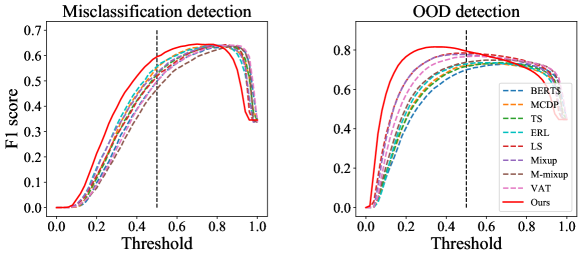
Figure 3: Calibration curves of OOD detection and misclassification detection on WOS. Our method can achieve high $F_{1}$ scores starting from a small threshold which indicates that it indeed provides low confidences for misclassified and OOD samples; the $F_{1}$ scores of the baselines peak at high thresholds which indicates that they are poorly calibrated.

Our main results are summarized as follows:

Expected Calibration Error: Table 1 reports the ECE and predictive accuracy of all the methods. Our method outperforms all the baselines on all the datasets in terms of ECE except for Yahoo, where only ERL is slightly better. Meanwhile, our method does not sacrifice the predictive accuracy.

Misclassification Detection: Table 2 compares the ${\rm NBAUCC}_{0.5}$ on misclassification detection of different methods. As shown, our method outperforms all the baselines on all the six datasets.

Out-of-distribution Detection: Table 2 reports the ${\rm NBAUCC}_{0.5}$ on OOD detection of different methods. Again, our method achieves the best performance on all the six datasets. The improvement is particularly remarkable on the 20NG dataset, where ${\rm NBAUCC}_{0.5}$ increases from $47.00$ to $63.92$ compared with the strongest baseline. We also find that detecting the unseen classes from the original dataset is much more challenging than detecting OOD samples from a totally different dataset.

Significance Test: We perform the Wilcoxon signed rank test (Wilcoxon, 1992) for significance test. For each dataset, we conduct experiments using 5 different random seeds with significance level $\alpha=0.5$. We find that our model outperforms other baselines on all the datasets significantly, with only exceptions of ERL in ECE on Yahoo and ERL in misclassification detection on 20NG.

Model	ECE						Accuracy
	20NG15	20NG	WOS100	WOS	Yahoo8	Yahoo	20NG15	20NG	WOS100	WOS	Yahoo8	Yahoo
BERT	$9.24$	$11.61$	$6.81$	$6.74$	$10.11$	$10.54$	$87.42$	$84.55$	$81.94$	$79.40$	$73.58$	$71.89$
TS	$4.42$	$8.17$	$3.63$	$4.43$	$5.18$	$4.24$	$87.42$	$84.55$	$81.94$	$79.40$	$73.58$	$71.89$
MCDP	$6.88$	$9.17$	$4.00$	$3.55$	$6.54$	$6.72$	$87.45$	$84.55$	$82.09$	$79.67$	$73.67$	$71.99$
LS	$4.35$	$6.15$	$4.35$	$4.67$	$4.89$	$3.61$	$87.54$	$85.02$	$81.95$	$79.47$	$73.66$	$71.54$
ERL	$7.16$	$6.10$	$3.74$	$3.35$	$3.42$	$\bm{2.96}$	$87.67$	$84.83$	$81.96$	$79.48$	$73.63$	$72.01$
VAT	$9.07$	$11.28$	$7.27$	$6.76$	$10.96$	$7.92$	$87.61$	$85.20$	$81.65$	$79.71$	$73.71$	$72.08$
Mixup	$5.98$	$9.02$	$4.72$	$4.21$	$4.60$	$5.18$	$87.49$	$84.86$	$81.97$	$79.51$	$73.88$	$71.82$
M-mixup	$5.04$	$7.78$	$6.48$	$6.68$	$7.01$	$6.07$	$87.40$	$84.45$	$81.77$	$79.57$	$73.67$	$72.03$
Ours	3.69	4.43	3.24	3.04	3.03	3.42	$87.44$	$84.53$	$81.59$	$79.06$	$73.71$	${72.17}$

Table 1: ECE and accuracy (in percentage). We report the average performance of 5 random initializations.

		Misclassification Detection					OOD Detection
Data	20NG15	20NG	WOS100	WOS	Yahoo8	Yahoo	20NG15	20NG	WOS100	WOS	Yahoo8	Yahoo
( OOD )							20NG5	SST-2	WOS34	AGnews	Yahoo2	Yelp
BERT	$2.30$	$2.86$	$16.53$	$20.52$	$7.47$	$8.43$	$2.66$	$21.65$	$23.12$	$49.84$	$8.35$	$13.88$
TS	$6.08$	$5.74$	$21.20$	$23.76$	$10.48$	$12.74$	$6.62$	$32.64$	$28.12$	$53.32$	$11.55$	$20.27$
MCDP	$4.37$	$5.28$	$20.44$	$24.16$	$10.12$	$10.75$	$3.99$	$25.10$	$27.28$	$53.52$	$9.98$	$15.93$
LS	$4.72$	$6.75$	$20.37$	$23.56$	$11.19$	$16.15$	$5.70$	$41.08$	$27.12$	$58.48$	$12.02$	$19.81$
ERL	$8.54$	$10.35$	$20.49$	$25.13$	$12.89$	$15.47$	$8.78$	$47.00$	$27.73$	$56.67$	$13.78$	$23.47$
VAT	$2.52$	$3.36$	$18.70$	$19.96$	$6.54$	$10.37$	$2.96$	$29.62$	$23.41$	$54.60$	$7.42$	$17.65$
Mixup	$4.99$	$4.51$	$20.65$	$24.80$	$10.75$	$11.29$	$5.86$	$31.84$	$26.77$	$58.02$	$11.62$	$19.84$
M-mixup	$2.16$	$3.16$	$16.94$	$19.39$	$9.09$	$11.79$	$2.36$	$26.08$	$24.08$	$51.39$	$10.08$	$22.41$
Ours	9.10	10.76	26.93	30.80	14.34	17.88	9.69	63.92	35.60	71.13	14.94	29.40

Table 2: ${\rm NBAUCC}_{0.5}$ on misclassification detection and OOD detection. We report the average performance of 5 random initializations.

4.5 Parameter Study

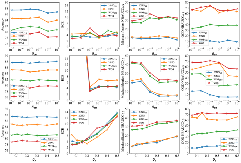
Figure 4: Parameter study of $\delta_{\rm on}$, $\delta_{\rm off}$ and $\delta_{y}$.

We investigate the effects of the interpolation parameters for on-manifold data, i.e., $\delta_{\rm on}$ and $\delta_{y}$, and the perturbation size for off-manifold samples, i.e., $\delta_{\rm off}$. The default values are $\delta_{\rm on}=10^{-4},\delta_{\rm off}=10^{-3}$ and $\delta_{y}=0.1$. Figure 4 shows the reuslts on 20NG₁₅, 20NG, WOS₁₀₀, and WOS datasets. Our results are summarized as follows:

$\bullet$ The performance of all metrics versus $\delta_{\rm on}$ is stable within a large range from $10^{-5}$ to $10^{-2}$. When $\delta_{\rm on}$ is larger than $10^{-1}$, the predictive accuracy begins to drop.

$\bullet$ The performance versus $\delta_{\rm off}$ is more sensitive: (1) when $\delta_{\rm off}$ is too small, ECE increases dramatically becasue the generated off-manifold samples are too close to the manifold and make the model under-confident. (2) when $\delta_{\rm off}$ is too large, the off-manifold regularization is too weak and OOD detection performance drops.

$\bullet$ In general, $\delta_{\rm on}$ should be small to let $\mathbf{x}^{\prime}$ stay on the data manifold while $\delta_{\rm off}$ should be large to let $\mathbf{x}^{\prime\prime}$ leave the data manifold. However, the regularization effect of $\mathcal{R}_{\rm on}$ ($\mathcal{R}_{\rm off}$) depends on both $\lambda_{\rm on}$ ($\lambda_{\rm off}$) and $\delta_{\rm on}$ ($\delta_{\rm off}$). Therefore, it is not necessary to let $\delta_{\rm on}$ be smaller than $\delta_{\rm off}$. We can also tune $\lambda_{\rm on}$ and $\lambda_{\rm off}$ to achieve better performance.

$\bullet$ The performance versus $\delta_{y}$ is relatively stable except for the metric of ECE. When $\delta_{y}$ is larger than $0.2$, ECE begins to increase.

4.6 Ablation Study

We investigate the effectiveness of the on-manifold regularizer $\mathcal{R}_{\rm on}$ and the off-manifold regularizer $\mathcal{R}_{\rm off}$ via ablation studies. Table 3 shows the results on the 20NG₁₅ and 20NG datasets.

$\bullet$ As expected, removing either component in our method would result in a performance drop. It demonstrates that these two components complement each other. All the ablation models outperform the BERT baseline model, which demonstrates the effectiveness of each module.

$\bullet$ We observe that the optimal $\delta_{\rm on}$ is different when using only $\mathcal{R}_{\rm on}$. This indicates that the hyperparameters of $\mathcal{R}_{\rm on}$ and $\mathcal{R}_{\rm off}$ should be jointly tuned, due to the joint effect of both components.

$\bullet$ By removing $\mathcal{R}_{\rm off}$, we observe a severe OOD performance degradation on the 20NG dataset (from 63.92 to 43.87). This indicates that $\mathcal{R}_{\rm off}$ is vital to out-of-distribution calibration. Meanwhile, the performance degradation is less severe on 20NG₁₅ (from 9.69 to 7.94). It is because $\mathcal{R}_{\rm on}$ can also help detect the OOD samples from similar data sources. (20NG₅).

$\bullet$ By removing $\mathcal{R}_{\rm on}$, the in-distribution calibration performance drops as expected.

Dataset		20NG15				20NG
Model	$\delta_{\rm on}$	Accuracy	ECE	OOD	Mis	Accuracy	ECE	OOD	Mis
BERT	-	$87.42$	$9.24$	$2.66$	$2.30$	$84.55$	$11.61$	$21.65$	$2.86$
w/ $\mathcal{R}_{\rm off}$	-	$86.48$	$6.51$	$6.22$	$6.09$	$83.90$	$7.98$	$55.40$	$7.12$
w/ $\mathcal{R}_{\rm on}$	$10^{-2}$	$88.73$	$2.77$	$7.94$	$8.08$	$85.60$	$5.00$	$35.80$	$8.66$
w/ $\mathcal{R}_{\rm on}$	$10^{-3}$	$88.29$	$3.52$	$7.39$	$6.83$	$85.69$	$4.43$	$38.00$	$9.01$
w/ $\mathcal{R}_{\rm on}$	$10^{-4}$	$87.93$	$4.48$	$5.33$	$4.83$	$85.12$	$6.76$	$43.87$	$5.95$
w/ $\mathcal{R}_{\rm on}$	$10^{-5}$	$87.61$	$4.69$	$3.83$	$4.73$	$85.39$	$6.35$	$35.70$	$5.30$
w/ Both	$10^{-4}$	$87.44$	$3.69$	$9.69$	$9.10$	$84.53$	$4.43$	$63.92$	$10.76$

Table 3: Ablation study on the 20NG₁₅ and 20NG datasets. For OOD detection and misclassification detection, we report BAUCC_0.5. We set $\delta_{y}=0.1$ and $\delta_{\rm off}=10^{-3}$.

5 Related Works and Discussion

Other Related Works: Lakshminarayanan et al. (2017) propose a model ensembling approach to improve model calibration. They first train multiple models with different initializations and then average their predictions. However, fine-tuning multiple language models requires extremely intensive computing resources.

Kumar et al. (2018) propose a differentiable surrogate for the expected calibration error, called maximum mean calibration error (MMCE), using kernel embedding. However, such a kernel embedding method is computationally expensive and not scalable to the large pre-trained language models.

Accelerating Optimization: To further improve the calibration performance of our method, we can leverage some recent minimax optimization techniques to better solve the two inner optimization problems in (5) and (7) without increasing the computational complexity. For example, Zhang et al. (2019) propose an efficient approximation algorithm based on Pontryagin’s Maximal Principle to replace the multi-step projected gradient update for the inner optimization problem. Another option is the learning-to-learn framework (Jiang et al., 2018), where the inner problem is solved by a learnt optimizer. These techniques can help us obtain $\mathbf{x}^{\prime}$ and $\mathbf{x}^{\prime\prime}$ more efficiently.

Connection to Robustness: The interpolated training samples can naturally promote the local Lipschitz continuity of our model. Such a local smoothness property has several advantages: (1) It makes the model more robust to the inherent noise in the data, e.g., noisy labels; (2) it is particularly helpful to prevent overfitting and improve generalization, especially for low-resource tasks.

Extensions: Our method is quite general and can be applied to other deep neural network-based problems besides language model fine-tuning.

6 Conclusion

We have proposed a regularization method to mitigate miscalibration of fine-tuned language models from a data augmentation perspective. Our method imposes two new regularizers using generated on- and off- manifold samples to improve both in-distribution and out-of-distribution calibration. Extensive experiments on six datasets demonstrate that our method outperforms state-of-the-art calibration methods in terms of expected calibration error, misclassification detection and OOD detection.

Appendix A Dataset Details

	#Train	#Dev	#Test	#Label
20NG15	7010	1753	5833	15
20NG5	-	-	1699	5
20NG	9051	2263	7532	20
SST-2	-	-	1822	2
WOS100	16794	4191	13970	100
WOS34	-	-	4824	34
WOS	22552	5639	18794	134
AGnews	-	-	7600	4
Yahoo8	16000	4000	48000	8
Yahoo2	-	-	12000	2
Yahoo	20000	5000	60000	10
Yelp	-	-	38000	2

Table 4: Dataset statistics and dataset split. ’-’ denotes that this part is not used. The original Yahoo dataset contains $140,000$ training samples for each class which is too large; we randomly draw $2,000$ and $500$ samples for each class as our training and development set.

All the data are publicly available. We also offer the links to the data as follows:

1. 20NG: http://qwone.com/~jason/20Newsgroups/.

2. SST-2: https://nlp.stanford.edu/sentiment/index.html.

3. WOS: https://data.mendeley.com/datasets/9rw3vkcfy4/2.

4. AGnews: https://github.com/yumeng5/WeSTClass.

5. Yahoo: https://www.kaggle.com/soumikrakshit/yahoo-answers-dataset.

6. Yelp: https://github.com/yumeng5/WeSTClass.

Appendix B Experiment Details

We use ADAM (Kingma and Ba, 2014) with $\beta_{1}=0.9$ and $\beta_{2}=0.999$ as the optimizer in all the datasets. We use the learning rate of $5\times 10^{-5}$ and batch size $32$ except $1\times 10^{-5}$ and $16$ for Yahoo₈ and Yahoo. We set the maximum number of epochs to 5 in Yahoo₈ and Yahoo and $10$ in the other datasets. We use the dropout rate of $0.1$ as in (Devlin et al., 2019). The documents are tokenized using wordpieces and are chopped to spans no longer than $150$ tokens on 20NG₁₅ and 20NG and 256 on other datasets..

Hyper-parameters: For our method, we use $\lambda_{\rm on}=\lambda_{\rm off}=1$, $\delta_{\rm on}=10^{-4}$, $\delta_{\rm off}=10^{-3}$ and $\delta_{y}=0.1$ for all the datasets. We then conduct an extensive hyper-parameter search for the baselines: for label smoothing, we search the smoothing parameter from $\{0.05,0.1\}$ as in (Müller et al., 2019); for ERL, the penalty weight is chosen from $\{0.05,0.1,0.25,0.5,1,2.5,5\}$; for VAT, we search the perturbation size in $\{10^{-3},10^{-4},10^{-5}\}$ as in (Jiang et al., 2020); for Mixup, we search the interpolation parameter from $\{0.1,0.2,0.3,0.4\}$ as suggested in (Zhang et al., 2018; Thulasidasan et al., 2019); for Manifold-mixup, we search from $\{0.2,0.4,1,2,4\}$. We perform 10 stochastic forward passes for MCDP at test time. For hyper-parameter tuning, we run all the methods 5 times and then take the average. The hyper-parameters are selected to get the best ECE on the development set of each dataset. The interpolation of Mixup is performed on the input embeddings obtained from the first layer of the language model; the interpolation of Manifold-mixup is performed on the features obtained from the last layer of the language model.

Appendix C Metrics of Misclassification and Out-of-distribution detection

Existing works on out-of-distribution (OOD) detection and misclassification detection (Hendrycks and Gimpel, 2016) use traditional binary classification metrics, e.g., AUPR and AUROC. As we discussed in Section 1 and 2, the output probability of a calibrated model should reflect the true likelihood. However, AUROC and AUPR cannot reflect true model calibration because the model can still achieve high scores even though it has high confidences for misclassified and OOD samples. We argue that it is more reasonable to use the Normalized Bounded Area Under the Calibration Curve (NBAUCC) defined as in Section 4.

Model	Confidence				Optimal $\tau$	AUPR	AUROC	${\rm NBAUCC}_{1}$	${\rm NBAUCC}_{0.5}$
	$x_{\rm in,1}$	$x_{\rm in,2}$	$x_{\rm out,1}$	$x_{\rm out,2}$
$h_{1}$ (Miscalibrated)	0.9	0.95	0.8	0.85	$(0.85,0.9)$	0.417	1	0.145	0
$h_{2}$ (Well-calibraterd)	0.9	0.95	0.1	0.15	$(0.15,0.9)$	0.417	1	0.845	0.773

Table 5: NBAUCC vs. AUROC/AUPR

Table 5 shows an illustrative example. As can be seen, $h_{1}$ is better calibrated than $h_{2}$, since $h_{1}$ can detect OOD samples under a wide range of threshold ($0.15<\tau<0.9$) while $h_{2}$ requires an absurdly large threshold ($0.85<\tau<0.9$). However, if we use the traditional AUPR and AUROC metrics, we will conclude that $h_{1}$ is as well calibrated as $h_{2}$ since AUPR^$h_{1}$ = AUPR^$h_{2}$ = $0.417$ and AUROC^$h_{1}$ = AUROC^$h_{2}$= $1$. On the other hand, if we use NBAUCC, we will have ${\rm NBAUCC}^{h_{1}}_{1}=0.845>{\rm NBAUCC}^{h_{1}}_{1}=0.145$, or ${\rm NBAUCC}^{h_{1}}_{0.5}=0.773>{\rm NBAUCC}^{h_{1}}_{0.5}=0$ which can reflect the true calibration of the two classifiers.

We remark that it is more appropriate to use ${\rm NBAUCC}_{0.5}$ than ${\rm NBAUCC}_{1}$ since a calibrated model should provide low confidences for the misclassified and OOD samples and it is unreasonable to use a large threshold to detect them.

Appendix D Additional Results

Table 6 and 7 report the NBAUCCs of all the methods on misclassification and OOD detection when $\tau_{\rm upper}=0.7$ and $\tau_{\rm upper}=1$. Table 8 and 9 report the ablation study results of all the methods when $\tau_{\rm upper}=0.7$ and $\tau_{\rm upper}=1$. Figure 5 and 6 report the parameter study results of all the methods when $\tau_{\rm upper}=0.7$ and $\tau_{\rm upper}=1$.

		Misclassification Detection					OOD Detection
Data	20NG15	20NG	WOS100	WOS	Yahoo8	Yahoo	20NG15	20NG	WOS100	WOS	Yahoo8	Yahoo
( OOD )							20NG5	SST-2	WOS34	AGnews	Yahoo2	Yelp
BERT	17.86	18.48	35.84	39.08	28.83	29.67	13.52	42.86	40.04	59.42	26.63	38.30
TS	23.74	23.58	38.34	40.76	31.10	32.63	19.74	50.00	42.96	60.70	28.30	42.07
MCDP	23.58	24.58	38.54	41.20	31.43	32.57	16.82	44.96	42.74	60.72	27.47	39.83
LS	21.22	23.24	37.22	40.12	30.93	34.30	18.76	55.24	42.54	63.62	27.87	40.77
ERL	24.04	25.68	37.87	41.17	32.27	33.90	22.10	54.20	42.67	62.10	28.73	43.37
VAT	17.80	17.50	35.90	38.80	27.87	31.13	13.00	49.00	40.30	62.50	25.80	40.63
Mixup	21.42	21.86	37.72	40.92	30.97	32.97	16.70	50.94	42.13	62.98	28.00	44.57
M-mixup	17.86	19.24	36.48	38.33	29.67	31.50	14.06	44.56	41.51	61.30	27.43	44.20
Ours	26.50	28.10	40.93	43.70	33.07	35.13	23.20	66.36	46.73	68.10	29.70	46.43

Table 6: $\rm NBAUCC_{1}$ on misclassification detection and OOD detection. We report the average performance of 5 random initializations.

		Misclassification Detection					OOD Detection
Data	20NG15	20NG	WOS100	WOS	Yahoo8	Yahoo	20NG15	20NG	WOS100	WOS	Yahoo8	Yahoo
( OOD )							20NG5	SST-2	WOS34	AGnews	Yahoo2	Yelp
BERT	8.26	8.70	26.95	31.18	18.52	19.46	7.05	33.24	32.97	57.45	18.86	27.68
TS	14.60	13.72	31.73	33.89	22.32	24.61	12.91	43.55	37.84	59.86	22.17	34.03
MCDP	13.14	14.21	31.05	34.74	21.41	22.62	9.85	36.96	36.97	60.06	19.99	29.45
LS	12.45	14.24	30.92	33.51	22.94	27.52	11.63	49.60	36.04	65.28	22.38	33.00
ERL	17.92	20.04	30.83	35.26	25.07	27.34	15.43	55.69	36.69	61.93	24.07	36.74
VAT	8.44	9.66	29.39	30.57	17.23	21.74	7.26	41.35	32.56	60.81	17.64	31.17
Mixup	13.33	11.87	31.71	35.24	22.62	22.80	11.50	43.60	37.09	65.51	22.19	33.66
M-mixup	8.67	9.89	27.33	29.61	20.33	23.05	7.18	37.10	33.57	58.13	20.66	36.42
Ours	18.35	20.18	36.63	40.01	25.94	29.15	16.55	68.72	43.40	72.62	25.03	41.11

Table 7: ${\rm NBAUCC}_{0.7}$ on misclassification detection and OOD detection. We report the average performance of 5 random initializations.

Dataset		20NG15				20NG
Model	$\delta_{\rm on}$	Accuracy	ECE	OOD	Mis	Accuracy	ECE	OOD	Mis
BERT	-	87.42	9.24	13.52	17.86	84.55	11.61	42.86	18.48
w/ $\mathcal{R}_{\rm off}$	-	86.48	6.51	18.10	24.53	83.90	7.98	63.73	25.40
w/ $\mathcal{R}_{\rm on}$	$10^{-2}$	88.73	2.77	22.83	27.40	85.60	5.00	51.53	27.40
w/ $\mathcal{R}_{\rm on}$	$10^{-3}$	88.29	3.52	21.03	24.13	85.69	4.43	53.87	26.30
w/ $\mathcal{R}_{\rm on}$	$10^{-4}$	87.93	4.48	17.43	21.63	85.12	6.76	57.47	21.93
w/ $\mathcal{R}_{\rm on}$	$10^{-5}$	87.61	4.69	15.73	21.43	85.39	6.35	52.07	21.63
w/ Both	$10^{-4}$	87.44	3.69	23.20	26.50	84.53	4.43	66.36	28.10

Table 8: Ablation study on the 20NG₁₅ and 20NG datasets. For OOD detection and misclassification detection, we report $\rm NBAUCC_{1}$. We set $\delta_{y}=0.1$ and $\delta_{\rm off}=10^{-3}$.

Dataset		20NG15				20NG
Model	$\delta_{\rm on}$	Accuracy	ECE	OOD	Mis	Accuracy	ECE	OOD	Mis
BERT	-	87.42	9.24	7.05	8.26	84.55	11.61	33.24	8.70
w/ $\mathcal{R}_{\rm off}$	-	86.48	6.51	11.75	14.79	83.90	7.98	62.67	15.42
w/ $\mathcal{R}_{\rm on}$	$10^{-2}$	88.73	2.77	15.27	18.35	85.60	5.00	46.67	18.39
w/ $\mathcal{R}_{\rm on}$	$10^{-3}$	88.29	3.52	13.86	15.66	85.69	4.43	50.07	18.17
w/ $\mathcal{R}_{\rm on}$	$10^{-4}$	87.93	4.48	10.61	12.59	85.12	6.76	53.64	13.18
w/ $\mathcal{R}_{\rm on}$	$10^{-5}$	87.61	4.69	8.71	12.25	85.39	6.35	46.24	12.20
w/ Both	$10^{-4}$	87.44	3.69	16.55	18.35	84.53	4.43	68.72	20.18

Table 9: Ablation study on the 20NG₁₅ and 20NG datasets. For OOD detection and misclassification detection, we report NBAUCC_0.7. We set $\delta_{y}=0.1$ and $\delta_{\rm off}=10^{-3}$.

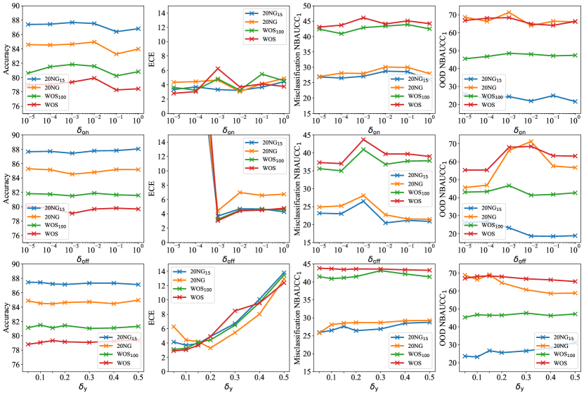
Figure 5: Parameter study of $\delta_{\rm on}$, $\delta_{\rm off}$ and $\delta_{y}$. We use ${\rm NBAUCC}_{1}$ for OOD and misclassification detection.

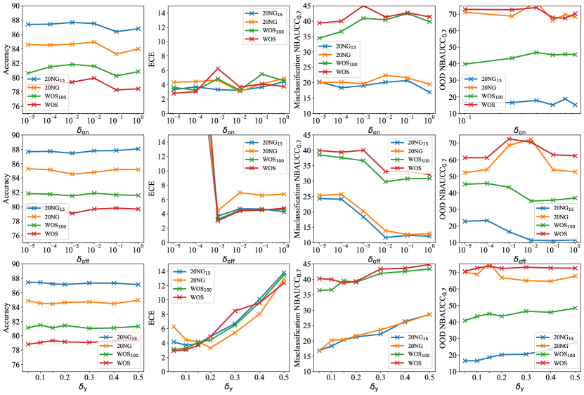
Figure 6: Parameter study of $\delta_{\rm on}$, $\delta_{\rm off}$ and $\delta_{y}$. We use ${\rm NBAUCC}_{0.7}$ for OOD and misclassification detection.

References

- Blundell et al. (2015) Blundell, C., Cornebise, J., Kavukcuoglu, K. and Wierstra, D. (2015). Weight uncertainty in neural network. In International Conference on Machine Learning.
- Chang et al. (2008) Chang, M.-W., Ratinov, L., Roth, D. and Srikumar, V. (2008). Importance of semantic representation: Dataless classification. In Proceedings of the Twenty-Third AAAI Conference on Artificial Intelligence.
- Chouldechova (2017) Chouldechova, A. (2017). Fair prediction with disparate impact: A study of bias in recidivism prediction instruments. Big data, 5 153–163.
- Devlin et al. (2019) Devlin, J., Chang, M.-W., Lee, K. and Toutanova, K. (2019). Bert: Pre-training of deep bidirectional transformers for language understanding. In Proceedings of the 2019 Conference of the North American Chapter of the Association for Computational Linguistics: Human Language Technologies, Volume 1 (Long and Short Papers).
- Gal and Ghahramani (2016) Gal, Y. and Ghahramani, Z. (2016). Dropout as a bayesian approximation: Representing model uncertainty in deep learning. In International Conference on Machine Learning.
- Gal et al. (2017) Gal, Y., Islam, R. and Ghahramani, Z. (2017). Deep bayesian active learning with image data. In International Conference on Machine Learning.
- Gilmer et al. (2018) Gilmer, J., Metz, L., Faghri, F., Schoenholz, S. S., Raghu, M., Wattenberg, M., Goodfellow, I. and Brain, G. (2018). The relationship between high-dimensional geometry and adversarial examples. arXiv preprint arXiv:1801.02774.
- Guo et al. (2017) Guo, C., Pleiss, G., Sun, Y. and Weinberger, K. Q. (2017). On calibration of modern neural networks. In International Conference on Machine Learning.
- Hendrycks and Gimpel (2016) Hendrycks, D. and Gimpel, K. (2016). A baseline for detecting misclassified and out-of-distribution examples in neural networks. In International Conference on Learning Representations.
- Jiang et al. (2018) Jiang, H., Chen, Z., Shi, Y., Dai, B. and Zhao, T. (2018). Learning to defense by learning to attack. arXiv preprint arXiv:1811.01213.
- Jiang et al. (2020) Jiang, H., He, P., Chen, W., Liu, X., Gao, J. and Zhao, T. (2020). SMART: Robust and efficient fine-tuning for pre-trained natural language models through principled regularized optimization. In Proceedings of the 58th Annual Meeting of the Association for Computational Linguistics.
- Kim (2014) Kim, Y. (2014). Convolutional neural networks for sentence classification. In Proceedings of the 2014 Conference on Empirical Methods in Natural Language Processing (EMNLP).
- Kingma and Ba (2014) Kingma, D. P. and Ba, J. (2014). Adam: A method for stochastic optimization. arXiv preprint arXiv:1412.6980.
- Kowsari et al. (2017) Kowsari, K., Brown, D. E., Heidarysafa, M., Jafari Meimandi, K., , Gerber, M. S. and Barnes, L. E. (2017). Hdltex: Hierarchical deep learning for text classification. In IEEE International Conference on Machine Learning and Applications (ICMLA).
- Kumar et al. (2018) Kumar, A., Sarawagi, S. and Jain, U. (2018). Trainable calibration measures for neural networks from kernel mean embeddings. In International Conference on Machine Learning.
- Lakshminarayanan et al. (2017) Lakshminarayanan, B., Pritzel, A. and Blundell, C. (2017). Simple and scalable predictive uncertainty estimation using deep ensembles. In Advances in Neural Information Processing Systems.
-
Lan et al. (2020)
Lan, Z., Chen, M., Goodman, S., Gimpel, K.,
Sharma, P. and Soricut, R. (2020).
Albert: A lite bert for self-supervised learning of language
representations.
In International Conference on Learning Representations.
https://openreview.net/forum?id=H1eA7AEtvS - Lee et al. (2018) Lee, K., Lee, K., Lee, H. and Shin, J. (2018). A simple unified framework for detecting out-of-distribution samples and adversarial attacks. In Advances in Neural Information Processing Systems.
- Liu et al. (2019) Liu, Y., Ott, M., Goyal, N., Du, J., Joshi, M., Chen, D., Levy, O., Lewis, M., Zettlemoyer, L. and Stoyanov, V. (2019). RoBERTa: A robustly optimized BERT pretraining approach. arXiv preprint arXiv:1907.11692.
- Louizos and Welling (2017) Louizos, C. and Welling, M. (2017). Multiplicative normalizing flows for variational Bayesian neural networks. In International Conference on Machine Learning.
- Miyato et al. (2018) Miyato, T., Maeda, S.-i., Koyama, M. and Ishii, S. (2018). Virtual adversarial training: a regularization method for supervised and semi-supervised learning. IEEE transactions on pattern analysis and machine intelligence, 41 1979–1993.
- Müller et al. (2019) Müller, R., Kornblith, S. and Hinton, G. E. (2019). When does label smoothing help? In Advances in Neural Information Processing Systems.
- Naeini et al. (2015) Naeini, M. P., Cooper, G. F. and Hauskrecht, M. (2015). Obtaining well calibrated probabilities using bayesian binning. In Proceedings of the Twenty-Ninth AAAI Conference on Artificial Intelligence.
- Niculescu-Mizil and Caruana (2005) Niculescu-Mizil, A. and Caruana, R. (2005). Predicting good probabilities with supervised learning. In International Conference on Machine Learning.
- Pereyra et al. (2017) Pereyra, G., Tucker, G., Chorowski, J., Kaiser, Ł. and Hinton, G. (2017). Regularizing neural networks by penalizing confident output distributions. arXiv preprint arXiv:1701.06548.
- Raffel et al. (2019) Raffel, C., Shazeer, N., Roberts, A., Lee, K., Narang, S., Matena, M., Zhou, Y., Li, W. and Liu, P. J. (2019). Exploring the limits of transfer learning with a unified text-to-text transformer. arXiv preprint arXiv:1910.10683.
- Shen et al. (2018) Shen, Y., Yun, H., Lipton, Z. C., Kronrod, Y. and Anandkumar, A. (2018). Deep active learning for named entity recognition. In International Conference on Learning Representations.
- Siddhant and Lipton (2018) Siddhant, A. and Lipton, Z. C. (2018). Deep bayesian active learning for natural language processing: Results of a large-scale empirical study. In Proceedings of the 2018 Conference on Empirical Methods in Natural Language Processing.
- Socher et al. (2012) Socher, R., Bengio, Y. and Manning, C. D. (2012). Deep learning for nlp (without magic). In Tutorial Abstracts of ACL 2012.
- Stutz et al. (2019) Stutz, D., Hein, M. and Schiele, B. (2019). Disentangling adversarial robustness and generalization. In Proceedings of the IEEE Conference on Computer Vision and Pattern Recognition.
- Thulasidasan et al. (2019) Thulasidasan, S., Chennupati, G., Bilmes, J. A., Bhattacharya, T. and Michalak, S. (2019). On mixup training: Improved calibration and predictive uncertainty for deep neural networks. In Advances in Neural Information Processing Systems.
- Verma et al. (2019) Verma, V., Lamb, A., Beckham, C., Najafi, A., Mitliagkas, I., Lopez-Paz, D. and Bengio, Y. (2019). Manifold mixup: Better representations by interpolating hidden states. In International Conference on Machine Learning.
- Wang et al. (2019) Wang, A., Pruksachatkun, Y., Nangia, N., Singh, A., Michael, J., Hill, F., Levy, O. and Bowman, S. (2019). Superglue: A stickier benchmark for general-purpose language understanding systems. In Advances in Neural Information Processing Systems.
- Wang et al. (2018) Wang, A., Singh, A., Michael, J., Hill, F., Levy, O. and Bowman, S. R. (2018). Glue: A multi-task benchmark and analysis platform for natural language understanding. In International Conference on Learning Representations.
- Wilcoxon (1992) Wilcoxon, F. (1992). Individual comparisons by ranking methods. In Breakthroughs in statistics. Springer, 196–202.
- Wong et al. (2019) Wong, E., Rice, L. and Kolter, J. Z. (2019). Fast is better than free: Revisiting adversarial training. In International Conference on Learning Representations.
- Zhang et al. (2019) Zhang, D., Zhang, T., Lu, Y., Zhu, Z. and Dong, B. (2019). You only propagate once: Accelerating adversarial training via maximal principle. In Advances in Neural Information Processing Systems.
- Zhang et al. (2018) Zhang, H., Cisse, M., Dauphin, Y. N. and Lopez-Paz, D. (2018). mixup: Beyond empirical risk minimization. In International Conference on Learning Representations.
- Zhang et al. (2015) Zhang, X., Zhao, J. and LeCun, Y. (2015). Character-level convolutional networks for text classification. In Advances in neural information processing systems.