Cluster-and-Conquer:
When Randomness Meets Graph Locality

Abstract

K-Nearest-Neighbors (KNN) graphs are central to many emblematic data mining and machine-learning applications. Some of the most efficient KNN graph algorithms are incremental and local: they start from a random graph, which they incrementally improve by traversing neighbors-of-neighbors links. Paradoxically, this random start is also one of the key weaknesses of these algorithms: nodes are initially connected to dissimilar neighbors, that lie far away according to the similarity metric. As a result, incremental algorithms must first laboriously explore spurious potential neighbors before they can identify similar nodes, and start converging. In this paper, we remove this drawback with Cluster-and-Conquer ($C^{2}$ for short). Cluster-and-Conquer boosts the starting configuration of greedy algorithms thanks to a novel lightweight clustering mechanism, dubbed FastRandomHash. FastRandomHash leverages randomness and recursion to pre-cluster similar nodes at a very low cost. Our extensive evaluation on real datasets shows that Cluster-and-Conquer significantly outperforms existing approaches, including LSH, yielding speed-ups of up to $\times 4.42$ while incurring only a negligible loss in terms of KNN quality.

I Introduction

$k$-Nearest-Neighbors (KNN) graphs play a fundamental role in many emblematic data-mining and machine-learning applications, including classification [1, 2], recommender systems [3, 4, 5, 6, 7], dimensionality reduction [8] and graph signal processing [9]. A KNN graph connects each node of a dataset to its $k$ closest counterparts (its neighbors), according to some application-dependent similarity metric. In many applications, this similarity is computed from a second set of entities, termed items, associated with each node. (For instance, if nodes are users, items might represent the websites they have visited.) Despite being one of the simplest models in data analysis, computing an exact KNN graph remains extremely costly, incurring, for instance, a quadratic number of similarity computations under a brute-force strategy.

Many applications, however, only require a reasonable approximation of a KNN graph, as long as this approximation can be produced rapidly. This is, for instance, true of online news recommenders, in which the use of fresh data is of utmost importance, or of machine learning techniques that use the KNN graph as a first preliminary step [8, 9]. Existing approximate KNN graph algorithms essentially fall into two families, that each uses different strategies to drastically reduce the number of similarities they compute: greedy incremental solutions [10, 3, 11, 12], and partition-based techniques (that include the popular LSH algorithm [13, 14]).

Greedy incremental solutions are currently among the best performing KNN graph construction algorithms, and exploit a local incremental search: they start from an initial random $k$-degree graph, which they greedily improve by traversing neighbors-of-neighbors links. Although they generally perform best, greedy approaches are critically hampered by their initial random start: similar nodes that lie close to one another in the final KNN graph are connected in the initial random graph to dissimilar nodes. In other words, these greedy approaches present a poor initial graph locality: nodes that are similar tend to be separated by long paths in the initial graph. As a result, greedy algorithms must initially compute many similarities between unrelated nodes, which adds a costly overhead for little to no benefit.

Partition-based algorithms [13, 14, 8] avoid this problem by clustering nodes before solving locally the problem, under a classic divide-and-conquer strategy. Unfortunately, a clustering that is both good and efficient is difficult to achieve. LSH [13, 14] for instance relies on hash functions that tend to fragment sparse datasets with large dimensions (from $\sim 10^{3}$ to $\sim 10^{5}$ in our experiments), which are typical of many on-line applications manipulating users and items. Traditional clustering techniques such as k-means [15] are similarly ill-fitted, as they require many similarity computations, which are precisely what we seek to avoid.

In this paper, we reconcile both perspectives with Cluster-and-Conquer ($C^{2}$ for short), a KNN graph algorithm for item-based datasets that boosts its initial graph locality by exploiting a novel, fast and accurate clustering scheme, dubbed FastRandomHash. FastRandomHash does not require any similarity computations (similarly to LSH) while avoiding fragmentation (similarly to k-means). FastRandomHash leverages fast random hash functions and employs a new recursive splitting mechanism to balance clusters, for optimal parallelism, and minimal synchronization between the involved threads in a parallel implementation.

We present an extensive evaluation of Cluster-and-Conquer, performed on six real datasets, which confirms that our proposal significantly outperforms existing approaches, including LSH, yielding speed-ups ranging from $\times 1.12$ (against LSH on MovieLens1M) to $\times 4.42$ (against Hyrec, a state of the art greedy KNN algorithm [3], on AmazonMovies) while incurring only a negligible loss in terms of KNN quality.

In the following, we first present the context of our work and our approach (Sec. II). We then formally analyze the novel clustering scheme at the core of our proposal (Sec. III). We present our evaluation procedure (Sec. IV) and our experimental results (Sec. IV); before reporting on factors impacting our solution (Sec. VI). We finally discuss related work (Sec. VII) and conclude (Sec. VIII).

II Cluster-and-Conquer

For ease of exposition, we consider in the following that nodes are users associated with items (e.g. web pages, movies, locations).

II-A Notations and problem definition

We note $U=\{u_{1},...,u_{n}\}$ the set of all users, and $I=\{i_{1},...,i_{m}\}$ the set of all items. The subset of items associated with user $u$ (a.k.a. her profile) is noted $\mathit{P}_{u}\subseteq I$. $\mathit{P}_{u}$ is generally much smaller than $I$ (the universe of all items).

Our objective is to approximate a k-nearest-neighbor (KNN) graph over $U$ (noted $G_{\operatorname{KNN}}$) according to some similarity function $sim\in\mathbb{R}^{U\times U}$ computed over user profiles:

$$sim(u,v)=f_{\mathit{sim}}(\mathit{P}_{u},\mathit{P}_{v})$$

where $f_{\mathit{sim}}$ may be any similarity function over sets that is positively correlated with the number of common items between the two sets, and negatively correlated with the total number of items present in both sets. These requirements cover some of the most commonly used similarity functions in KNN graph construction applications, such as cosine or the Jaccard similarity. We use the Jaccard similarity in the rest of the paper [16]:

$$sim(u,v)=J(P_{u},P_{v})=\frac{|P_{u}\cap P_{v}|}{|P_{u}\cup P_{v}|}$$

A KNN graph $G_{\operatorname{KNN}}$ connects each user $u\in U$ with a set $knn(u)$ (the ‘KNN’ of $u$ for short) which contains the k most similar users to $u$, with respect to the similarity function $sim(u,-)$.

Computing an exact KNN graph is particularly expensive: a brute-force exhaustive search requires $O(|U|^{2})$ similarity computations. Many scalable approaches, therefore, seek to construct an approximate KNN graph $\widehat{G}_{\operatorname{KNN}}$, i.e., to find for each user $u$ a neighborhood $\widehat{\mathit{knn}}(u)$ that is as close as possible to an exact KNN neighborhood [3, 11, 12]. The meaning of ‘close’ depends on the context, but in most applications, a good approximate neighborhood $\widehat{\mathit{knn}}(u)$ is one whose aggregate similarity (its quality) comes close to that of an exact KNN set $knn(u)$.

We capture how well the average similarity of an approximated graph $\widehat{G}_{\operatorname{KNN}}$ compares against that of an exact KNN graph $G_{\operatorname{KNN}}$ with the average similarity of $\widehat{G}_{\operatorname{KNN}}$, defined as the average similarity observed on the graph’s edges:

$$\mathit{avg\_sim}(\widehat{G}_{\operatorname{KNN}})=\frac{1}{k\times n}\sum\limits_{\begin{subarray}{c}(u,v)\in U^{2}:\\ \;v\in\widehat{\mathit{knn}}(u)\end{subarray}}f_{\mathit{sim}}(\mathit{P}_{u},\mathit{P}_{v}),$$ (1)

We then define the quality of $\widehat{G}_{\operatorname{KNN}}$ as the ratio between its average similarity and the average similarity of an exact KNN graph $G_{\operatorname{KNN}}$:

$$\mathit{quality}(\widehat{G}_{\operatorname{KNN}})=\frac{\mathit{avg\_sim}(\widehat{G}_{\operatorname{KNN}})}{\mathit{avg\_sim}(G_{\operatorname{KNN}})}.$$ (2)

A quality close to 1 indicates that the approximate KNN graph can replace the exact one with little impact in most applications.

With the above notations, we can summarize our problem as follows: for a given dataset $(U,I,(\mathit{P}_{u})_{u\in U})$ and item-based similarity $f_{\mathit{sim}}$, we wish to compute an approximate $\widehat{G}_{\operatorname{KNN}}$ in the shortest time with the highest overall quality.

II-B Intuition

Poor initial graph locality is a significant problem. Some of today’s best performing approaches for KNN graphs use a greedy strategy [3, 11, 12]: starting from a random initial $k$-degree graph, those algorithms incrementally seek to improve each user’s neighborhood by exploring neighbors-of-neighbors links. Unfortunately, this random start tends to separate similar nodes by long paths in the initial graph. This disconnect between similarity (which captures ‘closeness’ from the application’s point of view), and initial graph-distance (in terms of shortest path between two nodes), means greedy approaches initially suffer from a poor graph locality. This phenomenon is particularly marked in the first few iterations of greedy algorithms, in which neighbors-of-neighbors tend to be random, leading to spurious similarity computations, and a slow convergence [10].

Beyond convergence, a poor initial graph also hampers the concrete execution of greedy KNN graph approaches, for practical reasons linked to the memory management of modern computers. Because their initial graph is random, greedy approaches must iterate through users in an arbitrary order, usually employing parallelization (a.k.a. multithreading) on a multicore machine (as is typical for KNN graph computations). This arbitrary order prevents greedy approaches from fully exploiting the cache hierarchies of modern hardware: each thread accesses unrelated users, with unrelated profiles and neighborhoods, and cannot benefit from memory locality (the tendency of programs to access the same memory areas over short time windows). This low memory locality lowers the hit rates of processor caches and reduces performance.

Cluster-and-Conquer substantially improves the graph locality of its initial configuration, using an approximate, yet cheap and fast procedure. This basic principle is illustrated in Figure 1. Whereas standard greedy approaches (left) initially connect each user (in blue) to $k$ random neighbors (in red), Cluster-and-Conquer partitions users into small sub-datasets (also called clusters in the following), in which similar neighbors can be selected (Fig. 1b), leading to much faster computation times. We then assign each cluster to a dedicated thread, that computes its (partial) KNN graph in isolation, improving parallelism. Merging all resulting partial graphs produces the final global KNN graph.

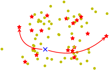
(a) Traditional greedy approaches

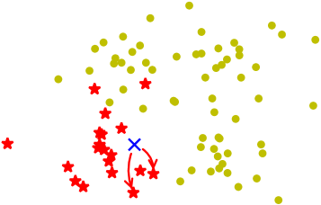
(b) Cluster-and-Conquer

Figure 1: Graph locality on a toy dataset (shown in 2D). A given user (in blue) starts with unrelated neighbors (in red) with traditional approaches (a). Cluster-and-Conquer ensures a much higher initial graph locality (b).

Clustering is key to both performance and quality. A core challenge when applying the above strategy consists in (i) grouping together similar users to produce good sub-datasets, while (ii) doing so on a tight computational budget. This is hard, as most clustering techniques for item-based datasets either tend to fragment users in a large number of buckets (e.g. LSH [13, 14]), or incur many similarity computations (e.g. k-means [15]).

Fast but approximate clustering does the job. To overcome this challenge, we introduce FastRandomHash, a novel, fast-to-compute hashing scheme that we use at the core of Cluster-and-Conquer to group users into highly-local and balanced sub-datasets. FastRandomHash does not require any similarity computation between users, yet remains extremely lightweight to compute. FastRandomHash exploits two ideas: (i) redundant random hashing on items for speed and graph locality, and (ii) recursive splitting for load balancing and parallelism.

Introducing redundancy to compensate for approximate clustering. Because we use random hash functions, similar nodes may still end up within different clusters, preventing them from becoming neighbors in the final global KNN graph, and resulting in a poor KNN approximation. To mitigate this risk, we use multiple hash functions, thus increasing the probability that similar neighbors end up within the same cluster at least once.

Recursively splitting large clusters to increase parallelism. By default, some clusters might become quite large, and slow down the whole computation. To avoid this problem, we introduce a recursive load balancing mechanism that exploits the same FastRandomHash scheme and repeatedly splits clusters that are larger than a given threshold $N$.

II-C Cluster-and-Conquer: Overview

Building on the previous intuitions, Cluster-and-Conquer works in three steps, which we present in detail in the remaining of this section:

• Step $\bf 1$: Clustering. The dataset is clustered in $t\times b$ clusters, using FastRandomHash functions, where $t$ is the number of hash functions, and $b$ the number of clusters per hash function. (We return later on to the effect of these two parameters on the algorithm’s speed and quality.) Clusters whose size exceeds $N$ are recursively split.

• Step $\bf 2$: Scheduling and KNN graph computation. The clusters are processed in parallel to produce a partial KNN for each of them. The parallel computation uses a greedy scheduling heuristic to balance work between computing cores.

• Step $\bf 3$: Merging. The resulting partial KNN graphs are merged.

The resulting KNN graph is returned as the KNN graph of the whole dataset.

II-D Step 1: Clustering with FastRandomHash

The FastRandomHash scheme first projects each item $i\in I$ onto a hash value $h(i)$ using a generative hash function $h:I\rightarrow\llbracket 1,b\rrbracket$. The hash $H(u)$ of a user $u$ is then taken as the minimum hash value among $u$’s items:

$$H(u)=\min_{i\in P_{u}}h(i).$$ (3)

For example, consider the following hash function $h$ over an item set $I=\{i_{1},i_{2},i_{3},i_{4},i_{5}\}$, with $b=3$.

$\begin{array}[]{c}\rotatebox[origin={c}]{-90.0}{$h$}\\ \overbrace{\hskip 50.00008pt}\end{array}$	$i_{1}\rightarrow 2$
	$i_{2}\rightarrow 3$
	$i_{3}\rightarrow 2$
	$i_{4}\rightarrow 1$
	$i_{5}\rightarrow 3$

If we apply FastRandomHash to two users $u$ and $v$ whose profiles are given as

$\mathit{P}_{u}=\{i_{1},i_{2},i_{3}\},$

$\mathit{P}_{v}=\{i_{3},i_{4},i_{5}\},$

we obtain, using the associated FastRandomHash $H$,

$H(u)=min\{h(i_{1}),h(i_{2}),h(i_{3})\}=min\{2,3,2\}=2,$

$H(v)=min\{h(i_{3}),h(i_{4}),h(i_{5})\}=min\{2,1,3\}=1,$

yielding the clustering configuration shown in Figure 2.

$\overbrace{\hskip 80.00012pt}^{\text{\normalsize{Cluster index}}}$
$1$		$2$		$3$
$v$		$u$

Figure 2: Clustering of $u$ and $v$ with $b=3$ clusters.

$H(u)$ determines $u$’s cluster under $h$, resulting in $b$ clusters for each generative function, what we have termed a clustering configuration. We use $t$ distinct generative functions, to produce $t$ clustering configurations and a total of $t\times b$ clusters. The use of multiple hash functions reduces the risk that two similar nodes are never hashed into the same cluster, an event whose probability decreases exponentially with the number of hash functions $t$.

As an example, consider the earlier example of Section II-D. We still have $I=\{i_{1},i_{2},i_{3},i_{4},i_{5}\}$ and $b=3$ and we are still interested in the two users $u$ and $v$. We rename the hash function $h$ by $h_{1}$ and $H$ by $H_{1}$. We consider another hash function $h_{2}$ and its associated FastRandomHash $H_{2}$:

$\begin{array}[]{c}\rotatebox[origin={c}]{-90.0}{$h_{2}$}\\ \overbrace{\hskip 50.00008pt}\end{array}$	$i_{1}\rightarrow 1$
	$i_{2}\rightarrow 3$
	$i_{3}\rightarrow 3$
	$i_{4}\rightarrow 2$
	$i_{5}\rightarrow 1$

$H_{2}(u)=min\{h_{2}(i_{1})=1,h_{2}(i_{2})=3,h_{2}(i_{3})=3\}=1$

$H_{2}(v)=min\{h_{2}(i_{3})=3,h_{2}(i_{4})=2,h_{2}(i_{5})=1\}=1$

	$\overbrace{\hskip 80.00012pt}^{\text{\normalsize{Cluster index}}}$
	$1$		$2$		$3$
$H_{1}$	$v$		$u$
$H_{2}$	$u,v$

Because $H_{1}(u)=2\neq H_{1}(v)=1$, users $u$ and $v$ are mapped into different clusters in the first hashing configuration defined by $H_{1}$, but as $H_{2}(u)=H_{2}(v)=1$, they appear in the same cluster in the second configuration corresponding to $H_{2}$. The fact that $u$ and $v$ share one item ($i_{3}$), means they have a non-zero probability of appearing in the same cluster, even though we use random hash functions. (We characterize this property more precisely in Section III.)

for $i\in\llbracket 1,t\rrbracket$ do $\rhd$$t$ hash functions

       $B_{i}\leftarrow\text{new }Set\langle U\rangle[b]()$

      

for $u\in U$ and $i\in\llbracket 1,t\rrbracket$ do $\rhd$clustering all users

       $B_{i}[H_{i}(u)]\leftarrow B_{i}[H_{i}(u)]\cup\{u\}$

        $\rhd$FastRandomHash

      

return $(B_{i})_{i\in\llbracket 1,t\rrbracket}$

Algorithm 1 Step $1$ of $C^{2}$: the clustering

Algorithm 1 shows the pseudocode of the clustering mechanism used by Cluster-and-Conquer. The variables $(C_{i})_{i\in\llbracket 1,t\rrbracket}$ are arrays of clusters. There are $t$ of them, one for each hash function. Each $C_{i}$ is of size $b$, the number of cluster per hash function $H_{i}$. Each $C_{i}[j]$ is a cluster, represented by a set of users, so that $\bigcup\limits_{j=1}^{b}C_{i}[j]=U$.

Balancing large clusters through recursive splitting. Using a minimum in the FastRandomHash function, unfortunately, introduces a bias towards the clusters of low indices. This bias is pervasive but particularly marked if highly popular items are hashed into one of the first clusters. In such a case, this cluster is likely to end up being much larger than the others in the same clustering configuration, many of which will be empty.

Highly unbalanced clusters tend to self-defeat the very purpose of the clustering step. This is because computing the partial KNN graph of a very large cluster can be almost as costly as that of the whole dataset. When this happens, the whole parallel computation is delayed, limiting the benefits of multi-threading. To avoid this situation, we recursively split overlarge clusters, by using the fact that FastRandomHash functions are extracted from hash values initially computed on items. More specifically, if a cluster $C$ with index $\eta_{C}$ is larger than a threshold parameter $N$, we compute a second FastRandomHash value $H\backslash\eta_{C}(u)$ for each of its users $u\in C$, by ignoring $C$’s index $\eta_{C}$ (i.e. the hash value that produced $C$) when computing the hash values of $u$’s items:

$$H\backslash\eta_{C}(u)=\min_{i\in P_{u},\,h(i)>\eta_{C}}h(i)$$

where $h$ is the generative hash function that underlies the clustering configuration containing $C$. The users of $C$ are then distributed among new clusters, one for each new hash value, with two exceptions. Users who have a single item (for whom $H\backslash\eta_{C}$ is undefined) and users who are alone in their new cluster remain in $C$. The resulting clusters are again recursively split if their size exceeds $N$. In summary, we split the users of a large cluster according to a second item, producing smaller and more refined clusters.

			$\overbrace{\hskip 80.00012pt}^{\text{\normalsize{Cluster index}}}$
			$1$		$2$		$3$
$\begin{array}[]{c}\begin{subarray}{c}\text{\normalsize Hash}\\ \text{\normalsize func.}\end{subarray}\\ \overbrace{\hskip 30.00005pt}\end{array}$	$H$		$75$		$10$		$15$
	$H\backslash 1$		$18$		$34$		$23$

Figure 3: Recursive splitting of clusters ($b=3$). In the initial clustering (first line), obtained with $H$, the first cluster $C_{H}[1]$ exceeds the threshold of $N=40$ users, and is therefore split, by applying $H\backslash 1$, which only keeps item hashes higher than $1$. Users with no items being hashed to $2$ or $3$ remain in the first cluster.

Figure 3 illustrates this recursive splitting strategy on a cluster configuration of $|U|=100$ users, $b=3$ and $N=40$. The first line represents the initial clustering, obtained with $H$, before the splitting. The boxes represent the clusters and the number in each box the size of the cluster. This initial clustering is highly unbalanced: the first cluster contains most of the users ($75$) while the others are nearly empty. Since its size is higher than $N=40$, the first cluster is split into new clusters, shown on the second line. The clusters of the second line are obtained using $H\backslash 1$, the FastRandomHash $H$ keeping only hashes higher than $1$, on the $75$ users. The first cluster is composed of users with no items being hashed to $2$ or $3$. As none of the new clusters contains more than $40$ users, the splitting stops. With the new clusters (shown in the second line), the new clustering configuration is more balanced, at the cost a few more clusters ($5$ instead of $3$).

The lower the threshold size $N$, the more balanced the final $t$ cluster configurations, thus the faster the computation. Still, small clusters increase the chance of similar users never appearing in the same cluster, potentially hurting the quality of the final global KNN graph. In practice, we choose $N=2000$.

II-E Comparison with LSH/MinHash

Although FastRandomHash can be understood as a randomized variant of the popular MinHash algorithm [17, 18], often used with LSH [13, 14], key differences in its design lead to starkly different properties. The use of random hash functions on a bounded discrete interval $\llbracket 1,b\rrbracket$ considerably reduces the resulting number of buckets (we use $b=4096$ by default in our experiments), which is otherwise determined by the size $|I|$ of the items universe with MinHash (which can be as high as 203,030 in the datasets we consider). Fewer buckets limit the dispersion of users in many small sub-datasets and increase the chances of finding good KNN neighbors while aligning better with the needs of a parallel implementation. Our choice of a small hashing space, however, tends to cause collisions and to produce unbalanced clusters.

Recursive splitting not only mitigates this second problem but also caps the maximum size of individual buckets, making the local KNN graph computations faster. Recursive splitting is also tightly linked to the small size of our hashing space. While it could in principle also be applied to MinHash, it would further fragment users into a still larger number of buckets, increasing the problem of dispersion mentioned earlier for the kind of sparse and large-dimensional datasets we consider.

II-F Step 2: Scheduling and local computation

Recursively splitting clusters reduces gross discrepancies between cluster sizes, but the final clusters might still remain unbalanced. To prevent an unbalanced workload among the threads of a parallel architecture, we apply some light-weight work scheduling. The clusters are stored in a synchronized, decreasing priority queue, ordered according to their size. We then use a basic thread pool to computes the KNN graph of each cluster in the queue, starting with the largest clusters and working down the priority queue until it becomes empty.

The partial KNN graph of each cluster $C$ can be computed using any approach and does not need to be synchronized with any other computation. In our prototype, we use a hybrid solution that switches between a brute force approach and a greedy KNN graph algorithm depending on the number of users $|C|$ in the cluster. (In practice we use Hyrec [3], see Sec. IV-B, but any other KNN graph algorithm can be used.) To determine a threshold value for the switch, we estimate the expected number of similarity computations for each approach and pick the least expensive. The brute force approach computes $\frac{|C|\times(|C|-1)}{2}$ similarities, while Hyrec’s number of similarities is bounded by $\frac{\rho\times k^{2}\times|C|}{2}$, where $\rho$ is the number of iterations. As a result, if $|C|<\rho\times k^{2}$ we choose the brute force approach, Hyrec otherwise. Algorithm 2 shows the pseudocode of the local KNN graph computation used by Cluster-and-Conquer. In practice, we take $\rho=5$. To further speed-up the computation, we use optimized versions of these algorithms that leverage a compact data structure [19] to provides a fast-to-compute estimation of Jaccard similarity values. In practice, this data structure, dubbed GoldFinger [19], summarizes each user’s profile into a 64- to 8096-bit vector, which is then used to estimate Jaccard similarity values.

if $|C|<\rho\times k^{2}$ then  return $BruteForce(C)$

else  return $Hyrec(C)$

Algorithm 2 Step 3 of $C^{2}$: local KNN on a cluster C

II-G Step 3: Merging the KNN graphs

Once the cluster phase is over, we merge the partial KNN graphs obtained for each cluster, one by one, into a unique KNN graph $knn$. Merging (Algorithm 3) is performed at the granularity of individual users. Each user appears in $t$ different clusters and is connected to up to $t\times k$ neighbors. For each cluster $C$, and each user $u$ of $C$, the KNN neighborhood $knn^{\prime}(u)$ of $u$ in $C$’s partial KNN graph is added to $u$’s final neighborhood $knn(u)$, while only keeping the $k$ best neighbors so far in $knn(u)$. While doing so we are careful to reuse similarity values, to avoid redundant computations. The resulting KNN graph $knn$ is returned.

$knn\leftarrow\text{new }knn()$

for $i\in\llbracket 1,t\rrbracket$ do $\rhd$for each hash function

       for $C\in\mathcal{C}_{i}$ do $\rhd$and for each cluster

             $knn^{\prime}\leftarrow C.knn()$

              $\rhd$compute the sub KNN for $C$

             for $u\in knn^{\prime}$ do $\rhd$merge this KNN into $knn(u)$

                   for $(v,s)\in knn^{\prime}(u)$ do

                         $knn(u).add(v,s)$

                        

                          $\rhd$$knn(u)$ is a heap bounded to size $k$

                        

                  

            

      

return $knn$

Algorithm 3 Step $4$ of $C^{2}$: KNN merging

III Theoretical Properties

The final neighbors of a user are selected from within the clusters in which this user appears. The quality of the final KNN graph is thus highly dependent on the ability of the hashing scheme to group similar users together. In the following, we prove that the probability of two users being hashed into the same bucket, before any splitting occurs, is proportional to their Jaccard similarity up to some small error introduced by collisions.

Theorem 1.

The probability $\mathbb{P}[H(u_{1})=H(u_{2})]$ that two users $u_{1}$, $u_{2}$ obtain the same FastRandomHash value $H(\cdot)$ is lower bounded by the following inequality

$$J_{1,2}-\frac{\kappa}{\ell}\leq\mathbb{P}[H(u_{1})=H(u_{2})],$$ (4)

where $J_{1,2}=J(P_{1},P_{2})$ is the Jaccard similarity between $u_{1}$’s and $u_{2}$’s profiles, $P_{1}$ and $P_{2}$; $\ell=|P_{1}\cup P_{2}|$ is the joint size of the two profiles; $\kappa=\ell-|h(P_{1}\cup P_{2})|$ is the overall number of collisions occurring when projecting the two profiles onto $\llbracket 1,b\rrbracket$, and $h(\cdot)$ is the generative hash function underpinning $H(\cdot)$. If we further assume $\kappa\leq\ell/2$, then we have

$$\mathbb{P}[H(u_{1})=H(u_{2})]\leq J_{1,2}+3\frac{\kappa}{\ell}+O\left(\frac{\kappa}{\ell}\right)^{2}.$$ (5)

Proof.

$\mathbb{P}[H(u_{1})=H(u_{2})]$ is proportional to $|h(P_{1})\cap h(P_{2})|$, where $h(X)$ is the image of the set $X$ by $h$. This is because $H(u_{1})=H(u_{2})$ iff the minimum element of $h(P_{1}\cup P_{2})$ happens to belong also to $h(P_{1})\cap h(P_{2})$. As the generative hash functions that send $P_{1}\cup P_{2}$ onto $h(P_{1}\cup P_{2})$ as $h$ does are each equally probable over the space of generative hash functions, the probability that the minimum element of $h(P_{1}\cup P_{2})$ belongs to $h(P_{1})\cap h(P_{2})$ is given by the ratio of the two sets’ sizes. More precisely:

$$\mathbb{P}[H(u_{1})=H(u_{2})]=\frac{|h(P_{1})\cap h(P_{2})|}{|h(P_{1}\cup P_{2})|}.$$ (6)

For brevity, let us note $P_{\cap}=P_{1}\cap P_{2}$ the set of items that are present in both profiles. Compared to $P_{\cap}$, collisions may both increase $h(P_{1})\cap h(P_{2})$ (if they occur between elements of $P_{1}\Delta P_{2}$, the symmetric difference of the users’ profiles, i.e. the items that only appear in one of the two profiles), or decrease it (if they occur between elements of $P_{\cap}$), yielding

$$|P_{\cap}|-\kappa\leq|h(P_{1})\cap h(P_{2})|\leq|P_{\cap}|+\kappa,$$ (7)

where $\kappa$ is the number of collisions caused by $h$ on $P_{1}\cup P_{2}$. Since by definition $|h(P_{1}\cup P_{2})|=\ell-\kappa$, we get

$$\frac{|P_{\cap}|/\ell-\kappa/\ell}{1-\kappa/\ell}\leq \mathbb{P}[H(u_{1})=H(u_{2})]\leq\frac{|P_{\cap}|/\ell+\kappa/\ell}{1-\kappa/\ell}$$ (8)

$$\frac{J_{1,2}-\kappa/\ell}{1-\kappa/\ell}\leq \mathbb{P}[H(u_{1})=H(u_{2})]\leq\frac{J_{1,2}+\kappa/\ell}{1-\kappa/\ell}.$$ (9)

Since $\kappa<\ell$, we trivially have $\frac{J_{1,2}-\kappa/\ell}{1-\kappa/\ell}\geq J_{1,2}-\frac{\kappa}{\ell}$, thus proving (4). If we assume $\kappa\leq\ell/2$, we can use the fact that $\frac{1}{1-x}\leq 1+2x$ when $x\in[0,\frac{1}{2}]$, which yields, together with $J_{1,2}\leq 1$

$$\frac{J_{1,2}+\kappa/\ell}{1-\kappa/\ell}\leq \left(J_{1,2}+\frac{\kappa}{\ell}\right)\left(1+2\frac{\kappa}{\ell}\right)\leq J_{1,2}+3\frac{\kappa}{\ell}+O\left(\frac{\kappa}{\ell}\right)^{2}$$

∎

Theorem 1 states that FastRandomHash will tend to allocate the same hash to similar users, modulo some noise introduced by collisions. In other words, the more similar two users are, the more likely they are to be allocated in the same clusters. We now bound the effect of collisions with the following concentration bound.

Theorem 2.

The collision density $\kappa/\ell$ is upper bounded by the value $(1+d)\frac{\ell-1}{2b}$ with a probability bounded by the following formula

$$\begin{array}[]{l}\displaystyle\mathbb{P}\left[\frac{\kappa}{\ell}<(1+d)\frac{\ell-1}{2b}\right]\geq 1-\left(\frac{e^{d}}{(1+d)^{(1+d)}}\right)^{\textstyle\frac{\ell(\ell-1)}{2b}},\end{array}$$ (11)

where $d>0$ is a real positive value, and the other variables are defined as in Theorem 1.

Proof.

If we imagine we project each element of $P_{1}\cup P_{2}$ one after the other, we can define $\ell$ random variables $(X_{k})_{\ell}$ that are equal to $1$ when the $k^{\mathrm{th}}$ element causes a collision, and to $0$ otherwise. We have $\kappa=\sum_{1\leq k\leq\ell}X_{k}$. By observing that $\mathbb{P}[X_{k}=1]\leq\frac{k}{b}$, we can define $\ell$ independent random variables $(X^{\prime}_{k})_{\ell}$, that are equal to $1$ with probability $\frac{k}{b}$, while upper bounding their corresponding $X_{k}$ in all realizations. As a result, $\kappa$ is upper bounded by their sum, which we note $S^{\prime}$,

$$\kappa\leq\sum_{1\leq k\leq\ell}X^{\prime}_{k}=S^{\prime}$$ (12)

We have $\mathbb{E}\left[S^{\prime}\right]=\sum_{k=0}^{\ell-1}\frac{k}{b}=\frac{\ell(\ell-1)}{2b}$. By applying the first Chernoff bound proposed by Mitzenmacher and Upfal [20] to $S^{\prime}$, we obtain the following concentration bound for S’:

$$\begin{array}[]{l}\displaystyle\mathbb{P}\left[S^{\prime}\geq(1+d)\frac{\ell(\ell-1)}{2b}\right]\leq\left(\frac{e^{d}}{(1+d)^{(1+d)}}\right)^{\textstyle\frac{\ell(\ell-1)}{2b}},\end{array}$$ (14)

where $d>0$ is a real positive value. Eq. (12) implies that $\mathbb{P}\left[\kappa\geq x\right]\leq\mathbb{P}\left[S^{\prime}\geq x\right]$ for any $x$. Applying this observation to (14) and taking the complement yields the theorem. ∎

As an example, if we apply Theorems 1 and 2 to the case of $\ell=256$, $b=4096$ (some typical values of our experiments), and set $d=0.5$ , we obtain that

$$J_{1,2}-0.078\leq\mathbb{P}[H(u_{1})=H(u_{2})]\leq J_{1,2}+0.234$$

with probability $0.998$ over the space of all hash functions $h$. The left-hand side of the above equation impacts the quality of our approximation, by ensuring that pairs of similar users tend to be compared: such users show a high $J_{1,2}$ value, and have therefore a high probability to be hashed to the same bucket, and to be compared, since this probability is lower-bounded by a value which is close to their Jaccard similarity. Conversely, the right-hand side controls the performance of our approach, by lowering the chances of comparing dissimilar users (and thus performing superfluous computations): the probability of such a comparison taking place is upper-bounded by $J_{1,2}$ (which is low for dissimilar users) plus a constant due to collisions that depends on $\ell$ and $b$ (0.234 in our numerical example).

IV Experimental Setup

TABLE I: Description of the datasets used in our experiments

Dataset	Users	Items	Scale	Ratings $>3$	$|P_{u}|$	$|P_{i}|$	Density
MovieLens1M (ml1M) [21]	6,038	3,533	1-5	575,281	95.28	162.83	2.697%
MovieLens10M (ml10M) [21]	69,816	10,472	0.5-5	5,885,448	84.30	562.02	0.805%
MovieLens20M (ml20M) [21]	138,362	22,884	0.5-5	12,195,566	88.14	532.93	0.385%
AmazonMovies (AM) [22]	57,430	171,356	1-5	3,263,050	56.82	19.04	0.033%
DBLP [23]	18,889	203,030	5	692,752	36.67	3.41	0.018%
Gowalla (GW) [24]	20,270	135,540	5	1,107,467	54.64	8.17	0.040%

IV-A Datasets

We use six publicly available users/items datasets (Table I) that cover a varied range of domains (movies and books reviews, co-authorship graphs, and geolocated social networks).

IV-A1 Three MovieLens datasets

MovieLens [21] is a group of anonymous datasets containing movie ratings collected on-line between 1995 and 2015 by GroupLens Research [25]. The datasets contain movie ratings on a $0.5$-$5$ scale by users who have at least performed more than $20$ ratings. To compute the Jaccard similarity, we binarize these datasets by keeping only ratings that reflect a positive opinion (i.e. higher than $3$). We use three versions of the dataset, MovieLens1M (ml1M), MovieLens10M (ml10M) and MovieLens20M (ml20M), containing between $575,281$ and $12,195,566$ positive ratings.

IV-A2 The AmazonMovies dataset

AmazonMovies [22] (AM) is a dataset of movie reviews from Amazon collected between 1997 and 2012. Ratings range from $1$ to $5$. We restrict our study to users with at least $20$ ratings (positive and negative ratings) to avoid dealing with users with not enough data (this problem, called the cold start problem, is generally treated separately [26]). After binarization, the resulting dataset contains $57,430$ users; $171,356$ items; and $3,263,050$ ratings.

IV-A3 DBLP

DBLP [23] is a dataset of co-authorship from the DBLP computer science bibliography. In this dataset, both the user set and the item set are subsets of the author set. If two authors have published at least one paper together, they are linked, which is expressed in our case by both of them appearing in the profile of the other with a rating of ‘5’. As with AM, we only consider users with at least $20$ ratings: the others are removed from the user set but not from the item set. The resulting dataset contains $18,889$ users, $203,030$ items, and $692,752$ ratings.

IV-A4 Gowalla

Gowalla [24] (GW) is a location-based social network. As DBLP, both user set and item set are subsets of the set of the users of the social network. The undirected friendship link from $u$ to $v$ is represented by $u$ rating $v$ with a $5$. As previously, only the users with at least $20$ ratings are considered. The resulting dataset contains $20,270$ users, $135,540$ items; and $1,107,467$ ratings.

We use all datasets for the main performance evaluation (Sec. V-A). We then focus on MovieLens10M and AmazonMovies for the parameter sensitivity analysis (Sec. VI). MovieLens10M and AmazonMovies have a similar number of users ($69,816$ for ml10M, $57,430$ for AM) and ratings ($5,885,448$ for ml10M, $3,263,050$ for AM) but they differ by the size of their item set ($10,472$ for ml10M against $171,356$ for AM): MovieLens10M is dense while AmazonMovies is sparse. This difference allows us to assess how sparsity impacts the performance and quality of Cluster-and-Conquer.

IV-B Baseline algorithms and competitors

We compare our approach against four competitors: a naive brute-force solution for reference, two state-of-the-art greedy KNN-graph algorithms (NNDescent [11, 12] and Hyrec [3]), and LSH [13]. On each dataset, we use the fastest competitor as our main baseline (termed ‘baseline’ or underlined in the following).

While many techniques exist to compute KNN graphs, the performance of most of them heavily depends on the properties of the dataset they are applied to. For example, product quantization [27] is designed to work well on datasets with a few hundred dimensions and dense values, i.e. in which each data point possesses a non-zero value in most dimensions. By contrast, our datasets are high-dimensional (ranging from $3,533$ to $203,030$ items), and sparse, containing only a few ratings per user, two characteristics that render them unsuitable for many existing KNN graph construction techniques. LSH remains the state of the art for KNN graphs computation in high-dimensional spaces and is routinely used as a baseline in recent works [28, 29, 30]. NNDescent experimentally outperforms LSH on high-dimensional datasets [11]. For a fair comparison, all competitors use the GoldFinger compact datastructure [19] to compute similarity values (Section II-F).

IV-B1 Brute force

The Brute Force competitor simply computes the similarities between every pair of profiles, performing a constant number of similarity computations equal to $\frac{n\times(n-1)}{2}$. This algorithm suffers from a high complexity, but produces an exact KNN graph.

IV-B2 Greedy approaches

NNDescent and Hyrec [3, 11, 12] are state-of-the-art greedy approaches that construct an approximate KNN graph by exploiting a local search strategy and by limiting the number of similarities computations. They start from an initial random graph, which is then iteratively refined until convergence. NNDescent [11, 12] and Hyrec [3] mainly differ in their iteration procedure. NNDescent compares all pairs $(u_{i},u_{j})$ among the neighbors of $u$, and updates the neighborhoods of $u_{i}$ and $u_{j}$ accordingly. By contrast, Hyrec compares all the neighbors’ neighbors of $u$ with $u$, rather than comparing $u$’s neighbors between themselves. Both algorithms stop either when the number of updates during one iteration is below the value $\delta\times k\times|U|$, with a fixed $\delta$, or after a fixed number of iterations.

IV-B3 LSH

Locality-Sensitive-Hashing (LSH) [13] reduces the number of similarity computations by hashing each user into several buckets. The neighbors of a user $u$ are then selected among the users present in the same buckets as $u$. To ensure that similar users tend to be hashed into the same buckets, LSH uses min-wise independent permutations of the item set as its hash functions, similarly to the MinHash algorithm [17]. For fairness, we implement LSH the same way as Cluster-and-Conquer: each hash function creates its own buckets, independently from each other, rather than having one bucket per item. This drastically decreases the number of similarity computations, resulting in a faster overall computation time while only inducing a small loss in quality.

IV-C Parameter setup

We compute KNN graphs with neighborhoods of size $k=30$, a standard value [11]. By default, when using Cluster-and-Conquer, the number of clusters per hash functions $b$ is set to $4096$ and the number of hash functions $t$ to $8$, except for DBLP and GW for which the number of hash functions is $15$. The maximum size of clusters for the recursive splitting procedure is set to $N=2000$, except for MovieLens20M for which it is $N=4000$. Both maximum sizes for clusters are below the threshold that determines whether BruteForce or Hyrec is used ($\rho\times k^{2}=4500$) in order to privilege Brute Force which tends to deliver better sub-KNNs than Hyrec. While locally computing the KNN graphs in clusters, we use 1024-bit GoldFinger vectors (See Section II-F). Beyond these default values, we present a detailed sensitivity study of the effect of $b$, $t$, and $N$ on the performance of Cluster-and-Conquer in Section VI-A.

The parameter $\delta$ of Hyrec and NNDescent is set to $0.001$, and their maximum number of iterations to $30$. The number of hash functions for LSH is 10.

IV-D Evaluation metrics

We measure the performance of Cluster-and-Conquer and its competitors along two main metrics: (i) their computation time, and (ii) the quality ratio of the resulting KNN (Sec. II-A). As an example of application, we also use the KNN graphs produced by Cluster-and-Conquer to compute recommendations and compare the resulting recall to recommendations obtained with an exact KNN graph computed with the brute force approach. Throughout our experiments, we use a 5-fold cross-validation procedure and average our results over the 5 resulting runs.

IV-E Implementation details and hardware

We have implemented Brute Force, Hyrec, NNDescent, LSH, and Cluster-and-Conquer in Java 1.8. Our FastRandomHash functions are computed using Jenkins’ hash function [31]. Our experiments run on a 64-bit Linux server with two Intel Xeon E5420@2.50GHz, totaling 8 hardware threads, 32GB of memory, and a HHD of 750GB. We use all 8 threads. Our code is available online.

V Evaluation

We first discuss the raw performance of Cluster-and-Conquer, compared to the brute force approach, LSH, NNDescent, and Hyrec (Sec. V-A). We then evaluate the performance of the obtained KNN graphs when used to provide recommendations (Sec. V-B). We evaluate the impact of FastRandomHash on Cluster-and-Conquer (Sec. V-C) and finally assess the effect of the GoldFinger data structure (Sec. V-D).

TABLE II: Computation time and KNN quality. Speed-ups are computed against the best baseline (underlined). Cluster-and-Conquer clearly outperforms all competitors, yielding speed-ups of up to $\times 4.42$ against the state of the art.

		Algo	Time (s)	Gain ($\%$)	Quality	$\Delta$
$\begin{array}[]{c}\mathit{datasets}\\ \overbrace{\hskip 256.50043pt}\end{array}$	ml1M	Hyrec	$4.43$	-	$0.92$	-
		NNDescent	$10.98$	-	$0.93$	-
		LSH	$2.96$	-	$0.92$	-
		$C^{2}$ (ours)	$\bf 2.64$	$10.81$	$0.91$	$-0.01$
	ml10M	Hyrec	$109.98$	-	$0.90$	-
		NNDescent	$147.03$	-	$0.93$	-
		LSH	$255.33$	-	$0.94$	-
		$C^{2}$	$\bf 27.79$	$74.73$	$0.89$	$-0.01$
	ml20M	Hyrec	$289.23$	-	$0.88$	-
		NNDescent	$383.21$	-	$0.92$	-
		LSH	$1060.76$	-	$0.93$	-
		$C^{2}$	$\bf 106.25$	$63.26$	$0.89$	$+0.01$
	AM	Hyrec	$62.41$	-	$0.93$	-
		NNDescent	$91.24$	-	$0.95$	-
		LSH	$140.53$	-	$0.96$	-
		$C^{2}$	$\bf 14.11$	$77.39$	$0.95$	$+0.02$
	DBLP	Hyrec	$26.84$	-	$0.81$	-
		NNDescent	$24.43$	-	$0.82$	-
		LSH	$37.80$	-	$0.86$	-
		$C^{2}$	$\bf 6.54$	$73.27$	$0.84$	$+0.02$
	GW	Hyrec	$21.88$	-	$0.78$	-
		NNDescent	$26.05$	-	$0.79$	-
		LSH	$26.91$	-	$0.82$	-
		$C^{2}$	$\bf 8.38$	$61.70$	$0.82$	$+0.04$

V-A Computation time and KNN quality

The performances of Cluster-and-Conquer are summarized in Table II over the six datasets. A part of the results is shown graphically in Figures 4 and 5. In addition to those of Cluster-and-Conquer (noted $C^{2}$), the performances of Hyrec, NNDescent, and LSH are also displayed for each dataset. The best computation time is shown in bold, the time of the best baseline is underlined, and the speed-up is computed w.r.t. this best baseline.

Cluster-and-Conquer provides the best computation time on all the datasets. Cluster-and-Conquer clearly outperforms all the approaches, providing speed-ups from $\times 1.12$ ($-10.81\%$ on ml1M) to $\times 4.42$ ($-77.39\%$ on AM) compared to the best baselines. The KNN quality provided by Cluster-and-Conquer is similar to the one provided by the fastest approaches: it goes from a loss of $0.01$ (on ml1M) to a gain of $0.04$ (on GW).

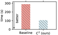
(a) MovieLens20M

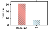
(b) AmazonMovies

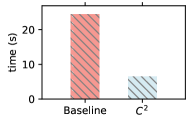
(c) DBLP

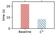
(d) Gowalla

Figure 4: Execution time of Cluster-and-Conquer ($C^{2}$) and the best competing approach (Baseline) for each dataset (lower is better). Cluster-and-Conquer clearly outperforms the best competitor across all datasets.

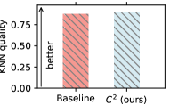
(a) MovieLens20M

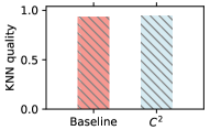
(b) AmazonMovies

(c) DBLP

(d) Gowalla

Figure 5: KNN quality using Cluster-and-Conquer and the fastest approach for each dataset (higher is better). Baseline refers to the fastest native approach. On the four above datasets, Cluster-and-Conquer ($C^{2}$) provides a slightly improved KNN quality.

TABLE III: Recommendation quality using the brute force approach and Cluster-and-Conquer ($C^{2}$) while recommending 30 items to every user. The loss in recall ($-2.05\%$ on average) incurred by Cluster-and-Conquer is small.

Dataset	Brute force	Cluster-and-Conquer	$\Delta$
MovieLens1M	$0.218$	$0.214$	$-0.004$
MovieLens10M	$0.273$	$0.271$	$-0.003$
MovieLens20M	$0.256$	$0.253$	$-0.003$
AmazonMovies	$0.595$	$0.570$	$-0.025$
DBLP	$0.360$	$0.355$	$-0.005$
Gowalla	$0.268$	$0.261$	$-0.007$

V-B Cluster-and-Conquer in action

We study the practical impact of the approximate KNN quality of Cluster-and-Conquer on the iconic item recommendation problem. We use a simple collaborative filtering procedure, and compare the recommendations obtained with exact KNN graphs to recommendations obtained with Cluster-and-Conquer. Table III shows the recall obtained when recommending $30$ items to each user in MovieLens1M, MovieLens10M, MovieLens20M, AmazonMovies, DBLP, and Gowalla using 5-fold cross-validation. The results of the exact KNN graphs are labeled BruteForce while the ones obtained with Cluster-and-Conquer are labeled $C^{2}$. The loss in recall is small: we obtain an average loss of $2.05\%$, with loss values ranging from $1.10\%$ on MovieLens10M to $4.20\%$ on AmazonMovies. Cluster-and-Conquer provides KNN graphs that are good enough to perform item recommendation with almost no loss, demonstrating its practical potential to accelerate end-user applications with close to no impact.

TABLE IV: Impact of the use of FastRandomHash functions (FRH for short) on Cluster-and-Conquer. The gain and speed-up values are computed against the best baseline of Table II. FastRandomHash functions provide important speeds-up at the cost of a small loss in KNN quality.

		Mechanisms	time (s)	Gain	Speed-up	Quality	$\Delta$
$\begin{array}[]{c}\textit{datasets}\\ \overbrace{\hskip 49.50008pt}\end{array}$	ml10M	MinHash	$126.74$	$-15.24\%$	$\times 0.87$	$0.93$	$+0.03$
		FRH (ours)	$\bf 27.79$	$74.73\%$	$\times 3.96$	$0.89$	$-0.01$
	AM	MinHash	$97.31$	$-55.90\%$	$\times 0.64$	$0.95$	$+0.02$
		FRH (ours)	$\bf 14.11$	$77.39\%$	$\times 4.42$	$0.95$	$+0.02$

V-C Impact of FastRandomHash

Cluster-and-Conquer combines several key mechanisms: FastRandomHash functions and their recursive splitting mechanism, the independent KNN computations, and the use of GoldFinger. To investigate the impact of FastRandomHash on the overall approach, we replace FastRandomHash with MinHash in Cluster-and-Conquer. MinHash functions are classically employed in the LSH algorithm and create one cluster per item by design. In the Cluster-and-Conquer/MinHash variant, we use $t$ MinHash functions to create $t\times m$ clusters, without splitting. The local KNN graphs are computed independently using GoldFinger on the $t\times m$ clusters, then merged as in Cluster-and-Conquer.

Table IV summarizes the results of all corresponding experiments. The table shows FastRandomHash has a decisive impact on the performance of our approach: it decreases the computation time by $78.07\%$ (MovieLens10M) and $85.50\%$ (AmazonMovies) while providing a competitive quality.

These results also demonstrate that Cluster-and-Conquer works well on both sparse and dense datasets, MovieLens10M and AmazonMovies being representative of both categories (see Sec. IV-A).

TABLE V: Impact of the use of GoldFinger functions (Golfi for short) on Cluster-and-Conquer. Gain and speed-up against the best baseline of Table II (with GoldFinger). GoldFinger provides an important speed-up to Cluster-and-Conquer, which remains nevertheless competitive even on raw data.

		Mechanisms	time (s)	Gain	Speed-up	Quality	$\Delta$
$\begin{array}[]{c}\textit{datasets}\\ \overbrace{\hskip 49.50008pt}\end{array}$	ml10M	Raw data	$111.29$	$-1.19\%$	$\times 0.99$	$0.94$	$+0.04$
		Golfi (ours)	$\bf 27.79$	$74.73\%$	$\times 3.96$	$0.89$	$-0.01$
	AM	Raw data	$35.05$	$43.84\%$	$\times 1.78$	$0.95$	$+0.02$
		Golfi (ours)	$\bf 14.11$	$77.39\%$	$\times 4.42$	$0.95$	$+0.02$

V-D Impact of GoldFinger

We now study the impact of GoldFinger on Cluster-and-Conquer by computing the KNN graphs both with GoldFinger and with the raw data. The results of these experiments are summarized in Table V. The gains and speed-ups are computed against the baselines of Table II (which use GoldFinger). Despite this disadvantage, Cluster-and-Conquer without GoldFinger is still competitive against the baselines, producing a $43.84\%$ gain in computation time on AmazonMovies, and being only slightly slower than the best competitor on MovieLens10M.

VI Sensitivity Analysis of Key Parameters

The performances of Cluster-and-Conquer depend on many parameters: the number of clusters per hash function, the number of hash functions, and the maximum size of the clusters. In this section, we study the influence of each of these parameters. Unless stated otherwise, the parameters are the same as in the previous sections: more specifically the number of clusters per hash function $b$ is $4096$, the number of hash functions $t$ is $8$, and the maximum size of the clusters $N$ is $2000$.

(a) MovieLens10M

(b) AmazonMovies

Figure 6: Effect of the number of hash functions $t$ on Cluster-and-Conquer, for MovieLens10M and AmazonMovies. Each curve shows the impact of $t$ as it takes the values $\{1,2,4,8,10\}$ for a given number of clusters $b\in\{512,2048,8192\}$. A higher $t$ trades off time for quality, but values beyond $8$ offer diminishing returns.

VI-A Number of clusters and hash functions

Figure 6 charts how Cluster-and-Conquer performs for three different values of $b$ ($512$, $2048$ and $8192$), and five values of $t$ ($1$, $2$, $4$, $8$, and $10$) on two time$\times$quality plots. Each curve corresponds to a given value of $b$, with the points of the curve obtained by varying $t$. The figure shows that $t$, the number of hash functions, captures a trade-off between computation time and KNN quality: more hash functions improve quality, but at the cost of higher computation times, and with diminishing returns beyond $t=8$.

In contrast to $t$, increasing $b$, the number of clusters per hash function, improves both the computation time and the KNN quality (albeit at the cost of a higher memory consumption). The impact of $b$ is more pronounced on AmazonMovies than on MovieLens10M. As we will see in the next section, this is probably because recursive splitting strongly impacts MovieLens10M and limits the influence of $b$ by adding a large number of additional clusters. By contrast, recursive splitting has no impact on AmazonMovies with $N=2000$ (the value used in Fig. 6), with the effect that the final number of clusters per hash function is solely determined by $b$.

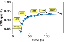
Figure 7: Effect of the maximum cluster size $N$ on the KNN quality and computing time of Cluster-and-Conquer on MovieLens10M. Reducing $N$ improves time at the expense of quality.

(a) MovieLens10M

(b) AmazonMovies

Figure 8: Effect of the maximum cluster size $N$ on the $100$ biggest clusters of Cluster-and-Conquer for MovieLens10M and AmazonMovies. On MovieLens10M, the biggest clusters have a size close to $N$ while $N\geq 1000$ has no impact on AM for which the biggest clusters have a size lower than $1000$.

VI-B The recursive splitting strategy

Figure 8 shows the impact of the maximum cluster size $N$ on the computation time and KNN quality of Cluster-and-Conquer on MovieLens10M when $N$ varies from $500$ to $10,000$. On MovieLens10M increasing $N$ leads to a higher KNN quality, but at the cost of a longer computation time, with a kneepoint around $N=3000$. By contrast, AmazonMovies shows almost no variation for the same values of $N$, and the corresponding plot is omitted for space reasons.

The difference in the impact of $N$ between MovieLens10M and AmazonMovies can be traced back to the popularity distribution of items in each dataset, which in turn impacts how the recursive splitting procedure affects each of them. This is illustrated in Figure 8, which shows the size of the $100$ biggest clusters in MovieLens10M and AmazonMovies for different values of $N$ ranging from $500$ to $10000$. In MovieLens10M (Fig. 8a), raw clusters (without splitting) are highly unbalanced (which is visible for high values of $N$ in the figure). As $N$ decreases, the size of the resulting clusters becomes more uniform, reducing computation times, but scattering similar users in distinct clusters, and thus hurting quality.

By contrast, the largest raw cluster in AmazonMovies (Fig. 8b) contains fewer than $1000$ users. As a result, except for the smallest value of $N=500$, Cluster-and-Conquer on AmazonMovies does not use recursive splitting and is immune to the impact of $N$.

VII Related Work

KNN graphs are a key mechanism in many problems ranging from classification [1, 2] to item recommendation [3, 4, 5]. Also, KNN graphs are the first step of more advanced machine-learning techniques [8].

In small dimension, i.e. when the item set is small, the computation of an exact KNN graph is achieved with specialized data structures [32, 33, 34]. In high dimension, these techniques are more expensive than the brute force approach. Computing an exact KNN graph efficiently in high dimension remains an open problem.

To speed-up the computation of the KNN graph in high dimension, recent approaches decrease the number of similarities computed. In LSH [13, 14], each user is placed into several buckets, depending on their profiles. Two users are in the same bucket with a probability proportional to their similarity. The KNN of each user is then computed by only considering the users who are in the same buckets as her. Unfortunately, LSH [13, 14] tends to scale poorly when applied to datasets with large item sets.

Greedy approaches [3, 11, 12] reduce the number of computing similarities by performing a local search: they assume that neighbors of neighbors are also likely to be neighbors. They start from a random graph and then iteratively refine each neighborhood by computing similarities among neighbors of neighbors. These approaches are the most efficient so far on the datasets we are working on. Still, they spend most of the total computation time computing similarities [10].

Compact representations of the data can be used to speed-up similarity computations. Several estimators [35, 36], including the popular MinHash [17, 18], rely on compact datastructures to provide a quick yet accurate estimate of the Jaccard similarity. Bloom filters [37] can be used as a compact representation of the users’ profiles while computing a KNN graph [38, 1]. Another very simple approach consists in limiting the size of each user’s profile by sampling [39]. GoldFinger [40] is a fast-to-compute compact data structure designed to speed up the Jaccard similarity, which has shown good results across a range of datasets and algorithms [19].

Among the classical clustering techniques, k-means [15] relies on similarities to provide an efficient clustering: [41] uses a k-means to cluster the users before computing locally the KNN graph. Unfortunately, it requires to compute many similarities while our main purpose is to limit as much as possible the number of similarities computed. On the other hand, LSH [13, 14] clusters users without computing any similarity. The work presented in [42] uses LSH to cluster users before computing local KNN graphs, as we do. The complexity of their clustering approach is $O(n\times m)$, where $n$ is the number of items and $m$ the number of features. The performances are good in image datasets, where the dimension $m$, i.e. the number of pixels, is a few thousand but it becomes prohibitive on datasets with much higher dimensions, such as the examples with have considered here. Similarly, the use of recursive Lanczos bisections [8, 43] leverages a similar strategy but the divide step has a complexity that makes it more expensive than the brute force approach when used with high dimensional datasets such as the ones we consider.

VIII Conclusions

In this paper, we have proposed Cluster-and-Conquer, a novel algorithm to compute KNN graphs. Cluster-and-Conquer accelerates the construction of KNN graphs by approximating their graph locality in a fast and robust manner. Cluster-and-Conquer relies on a divide-and-conquer approach that clusters users, computes locally the KNN graphs in each cluster, and then merges them. The novelties of the approach are the FastRandomHash functions used to pre-cluster users, their recursive splitting mechanism to produced more balanced clusters, and the fact that the clusters are computed independently, without any synchronization. Although we have only considered standalone experiments, the general structure of Cluster-and-Conquer further makes is particularly amenable to large-scale distributed deployments, in particular within a map-reduce infrastructure.

We extensively evaluated Cluster-and-Conquer on real datasets and conducted a sensitivity analysis. Our results show that Cluster-and-Conquer significantly outperforms the best existing approaches, including LSH, on all datasets, yielding speed-ups ranging from $\times 1.12$ (against Hyrec on ml1M) up to $\times 4.42$ (against Hyrec on AM), while incurring only negligible losses in KNN quality. Finally, we showed that the obtained graphs can replace the exact ones when performing recommendations with almost no discernible impact on recall.

References

- [1] M. Gorai, K. Sridharan, T. Aditya, R. Mukkamala, and S. Nukavarapu, “Employing bloom filters for privacy preserving distributed collaborative knn classification,” in WICT, 2011.
- [2] N. Nodarakis, S. Sioutas, D. Tsoumakos, G. Tzimas, and E. Pitoura, “Rapid aknn query processing for fast classification of multidimensional data in the cloud,” CoRR, 2014.
- [3] A. Boutet, D. Frey, R. Guerraoui, A.-M. Kermarrec, and R. Patra, “Hyrec: leveraging browsers for scalable recommenders,” in Middleware, 2014.
- [4] J. J. Levandoski, M. Sarwat, A. Eldawy, and M. F. Mokbel, “Lars: A location-aware recommender system,” in ICDE, 2012.
- [5] G. Linden, B. Smith, and J. York, “Amazon. com recommendations: Item-to-item collaborative filtering,” Internet Computing, IEEE, 2003.
- [6] B. Sarwar, G. Karypis, J. Konstan, and J. Riedl, “Item-based collaborative filtering recommendation algorithms,” in WWW, 2001.
- [7] P. G. Campos, A. Bellogín, F. Díez, and J. E. Chavarriaga, “Simple time-biased knn-based recommendations,” in Workshop on Context-Aware Movie Recommendation, 2010.
- [8] J. Chen, H.-r. Fang, and Y. Saad, “Fast approximate knn graph construction for high dimensional data via recursive lanczos bisection,” Journal of Machine Learning Research, 2009.
- [9] N. Tremblay, G. Puy, P. Borgnat, R. Gribonval, and P. Vandergheynst, “Accelerated spectral clustering using graph filtering of random signals,” in ICASSP, 2016.
- [10] A. Boutet, A.-M. Kermarrec, N. Mittal, and F. Taïani, “Being prepared in a sparse world: the case of knn graph construction,” in ICDE, 2016.
- [11] W. Dong, C. Moses, and K. Li, “Efficient k-nearest neighbor graph construction for generic similarity measures,” in WWW, 2011.
- [12] B. Bratić, M. E. Houle, V. Kurbalija, V. Oria, and M. Radovanović, “NN-Descent on high-dimensional data,” in WIMS, 2018.
- [13] P. Indyk and R. Motwani, “Approximate nearest neighbors: towards removing the curse of dimensionality,” in STOC, 1998.
- [14] A. Gionis, P. Indyk, R. Motwani et al., “Similarity search in high dimensions via hashing,” in VLDB, 1999.
- [15] J. MacQueen et al., “Some methods for classification and analysis of multivariate observations,” in Fifth Berkeley Symp. on Math. Statistics and Prob., 1967.
- [16] C. J. van Rijsbergen, Information retrieval. Butterworth, 1979.
- [17] A. Z. Broder, “On the resemblance and containment of documents,” in Compression and Complexity of Sequences, 1997.
- [18] P. Li and A. C. König, “Theory and applications of b-bit minwise hashing,” Communications of the ACM, 2011.
- [19] R. Guerraoui, A.-M. Kermarrec, O. Ruas, and F. Taïani, “Smaller, faster & lighter knn graph constructions,” in WWW, 2020.
- [20] M. Mitzenmacher and E. Upfal, Probability and computing: Randomization and probabilistic techniques in algorithms and data analysis. Cambridge university press, 2017.
- [21] F. M. Harper and J. A. Konstan, “The movielens datasets: History and context,” ACM Trans. Interact. Intell. Syst., 2015.
- [22] J. J. McAuley and J. Leskovec, “From amateurs to connoisseurs: modeling the evolution of user expertise through online reviews,” in WWW, 2013.
- [23] J. Yang and J. Leskovec, “Defining and evaluating network communities based on ground-truth,” CoRR, vol. abs/1205.6233, 2012.
- [24] E. Cho, S. A. Myers, and J. Leskovec, “Friendship and mobility: User movement in location-based social networks,” in KDD, 2011.
- [25] P. Resnick, N. Iacovou, M. Suchak, P. Bergstrom, and J. Riedl, “Grouplens: an open architecture for collaborative filtering of netnews,” in ACM Conf. on Computer Supported Cooperative Work, 1994.
- [26] X. N. Lam, T. Vu, T. D. Le, and A. D. Duong, “Addressing cold-start problem in recommendation systems,” in 2nd Int. Conf. on Ubiquitous Information Management and Comm., 2008.
- [27] H. Jegou, M. Douze, and C. Schmid, “Product quantization for nearest neighbor search,” IEEE Trans. on Pattern Analysis and Machine Intelligence, 2010.
- [28] W. Liu, H. Wang, Y. Zhang, W. Wang, and L. Qin, “I-LSH: I/O efficient c-approximate nearest neighbor search in high-dimensional space,” in ICDE, 2019.
- [29] B. Zheng, X. Zhao, L. Weng, N. Q. V. Hung, H. Liu, and C. S. Jensen, “PM-LSH: A fast and accurate lsh framework for high-dimensional approximate nn search,” Proceedings of the VLDB Endowment, 2020.
- [30] D. Cai, “A revisit of hashing algorithms for approximate nearest neighbor search,” IEEE Trans. on Knowledge and Data Engineering, 2019.
- [31] B. Jenkins, “Hash functions,” Dr Dobbs Journal, 1997.
- [32] J. L. Bentley, “Multidimensional binary search trees used for associative searching,” Comm. ACM, 1975.
- [33] A. Beygelzimer, S. Kakade, and J. Langford, “Cover trees for nearest neighbor,” in ICML, 2006.
- [34] T. Liu, A. W. Moore, K. Yang, and A. G. Gray, “An investigation of practical approximate nearest neighbor algorithms,” in NIPS, 2004.
- [35] S. Dahlgaard, M. B. T. Knudsen, and M. Thorup, “Fast similarity sketching,” in 2017 IEEE 58th Annual Symposium on Foundations of Computer Science (FOCS), 2017.
- [36] T. Christiani, R. Pagh, and J. Sivertsen, “Scalable and robust set similarity join,” in 2018 IEEE 34th International Conference on Data Engineering (ICDE), 2018.
- [37] B. H. Bloom, “Space/time trade-offs in hash coding with allowable errors,” Communications of the ACM, 1970.
- [38] M. Alaggan, S. Gambs, and A.-M. Kermarrec, “Blip: Non-interactive differentially-private similarity computation on bloom filters.” in SSS, 2012.
- [39] A. Kermarrec, O. Ruas, and F. Taïani, “Nobody cares if you liked star wars: KNN graph construction on the cheap,” in Euro-Par’18, 2018.
- [40] R. Guerraoui, A. Kermarrec, O. Ruas, and F. Taïani, “Fingerprinting big data: The case of knn graph construction,” in ICDE, 2019.
- [41] G.-R. Xue, C. Lin, Q. Yang, W. Xi, H.-J. Zeng, Y. Yu, and Z. Chen, “Scalable collaborative filtering using cluster-based smoothing,” in SIGIR. ACM, 2005.
- [42] Y. Zhang, K. Huang, G. Geng, and C. Liu, “Fast kNN graph construction with locality sensitive hashing,” in ECML/PKDD, 2013.
- [43] C. Lanczos, An iteration method for the solution of the eigenvalue problem of linear differential and integral operators. United States Governm. Press Office, Los Angeles, CA, 1950.