Quasiperiodic Floquet-Thouless energy pump

Abstract

We study a disordered one-dimensional fermionic system subject to quasiperiodic driving by two modes with incommensurate frequencies. We show that the system supports a topological phase in which energy is transferred between the two driving modes at a quantized rate. The phase is protected by a combination of disorder-induced spatial localization and frequency localization, a mechanism unique to quasiperiodically driven systems. We demonstrate that an analogue of the phase can be realized in a cavity-qubit system driven by two incommensurate modes.

Periodic driving can be used as a tool for quantum control Vandersypen and Chuang (2005); Bukov et al. (2015); Weinberg et al. (2017); Lindner et al. (2011); Struck et al. (2012); Wang et al. (2013); Jotzu et al. (2014); McIver et al. (2020); Viola and Lloyd (1998); Viola et al. (1999); de Lange et al. (2010); Dalibard et al. (2011); Struck et al. (2011); Goldman and Dalibard (2014) and can even induce new phases of matter with no equilibrium analogues Jiang et al. (2011); Rudner et al. (2013); Nathan and Rudner (2015); Khemani et al. (2016); von Keyserlingk C. W. and Sondhi (2016a, b); Kitagawa et al. (2010); Rudner et al. (2013); Titum et al. (2016); Nathan et al. (2017, 2019a); Wintersperger et al. (2020); Sacha (2015); Else et al. (2016); Yao et al. (2017); Zhang et al. (2017); Choi et al. (2017). Recently, it was discovered that quasiperiodically driven systems also support their own unique phases of matter Else et al. (2020), despite having neither continuous nor discrete time-translation symmetry.

In this work, we report the discovery of a topological phase of matter in quasiperiodically driven systems. We study a one-dimensional (1d) fermionic system driven by two modes with incommensurate frequencies, $\omega_{1}$ and $\omega_{2}$. With spatial disorder, the system supports a phase which is characterized by quantized energy transport and a nonzero value of an integer-valued topological invariant $\nu$. When one end of the system is fully occupied by fermions while the other end is empty [as depicted in Fig. 1(a)], the system transfers energy between the driving modes at the quantized average rate $\nu\mathcal{P}_{0}$, where $\mathcal{P}_{0}\equiv{\omega_{1}\omega_{2}}/{2\pi}$ denotes the “quantum of energy transfer” (with $\hbar=1$ throughout). We refer to this phase as the quasiperiodic Floquet-Thouless energy pump (QFTEP).

The absence of time-translation symmetry gives the QFTEP features which have no analogue in equilibrium or Floquet systems. In particular, the QFTEP is protected by a combination of spatial and frequency localization Ho et al. (1983); Luck et al. (1988); Casati et al. (1989); Blekher et al. (1992); Hatami et al. (2016); Else et al. (2020), meaning the index $\nu$ can only change if this localization is destroyed. Here frequency localization is a phenomenon unique to quasiperiodically driven systems which arises only for sufficiently irrational $\omega_{2}/\omega_{1}$. The condition of irrational $\omega_{2}/\omega_{1}$ means the QFTEP features a fractally-structured phase diagram (see Fig. 2 and discussion below for details).

The same “quantum of energy transfer” that we observe was recently encountered in Refs. Kolodrubetz et al. (2018); Martin et al. (2017); Nathan et al. (2019b). In particular, Ref. Kolodrubetz et al. (2018) studied the same class of systems we consider here, in the limit where the second driving mode is adiabatic: $\omega_{2}\to 0$. For fine-tuned parameters, and in the absence of disorder, this system was shown to exhibit a similar quantized energy pumping phenomenon to that we observe here. Unlike the phenomena in Refs. Kolodrubetz et al. (2018); Martin et al. (2017); Nathan et al. (2019b), the QFTEP does not require adiabatic driving, is robust to disorder, and occupies a finite region of parameter space. Hence the QFTEP, in contrast to these earlier phenomena, constitutes a genuine phase of matter.

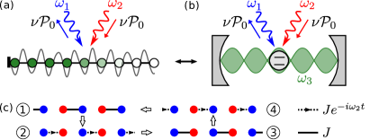
Figure 1: (a) The quasiperiodic Floquet-Thouless energy pump for a fermionic chain driven by incommensurate frequencies $\omega_{1}$ and $\omega_{2}$. When one end of the chain is fully occupied (green), energy is pumped between the two modes at the rate $\nu\mathcal{P}_{0}$ ($\mathcal{P}_{0}=\omega_{1}\omega_{2}/2\pi$), where $\nu\in\mathds{Z}$ is the topological winding number of the phase. The quantization persists as long as the system is localized in both real and frequency space. (b) An analogue of the phase can be realized with a bichromatically driven qubit-cavity system. (c) $4$-step driving protocol that realizes the phase. A particle tunneling along (against) the arrow acquires a phase $e^{-i\omega_{2}t}$ ($e^{i\omega_{2}t}$).

We propose an experimental realization of a dimensionally-reduced version of the QFTEP in a two-level system (qubit) coupled to a quantized cavity mode and driven by two incommensurate frequencies [see Fig. 1(b)]. Our results indicate that such a simple physical setup inherits the topological properties of the QFTEP, suggesting the possibility of realizing this phase in cavity quantum electrodynamics.

Model — Here we present a particular model that realizes the QFTEP. We consider a 1d bipartite tight-binding system with $L$ unit cells, with Hamiltonian $\hat{\mathcal{H}}_{0}(t{;\lambda})=\hat{\mathcal{H}}_{\rm dr}(t{;\lambda})+\hat{\mathcal{H}}_{\mathrm{dis}}$. Here, for fixed $\lambda\in\mathbb{R}$, $\hat{\mathcal{H}}_{\rm dr}(t;\lambda)$ describes time-dependent tunneling with period $T_{1}$, while $\hat{\mathcal{H}}_{\rm dis}=\sum_{x=1}^{2L}\frac{\Delta_{x}}{2}\hat{c}^{\dagger}_{x}\hat{c}_{x}$ describes a static on-site disorder potential. Here $\hat{c}_{x}$ annihilates a fermion on site $x$, while each $\Delta_{x}$ is picked randomly from the interval $[-W,W]$. We take the lattice constant to be $1$ throughout. The driving term $\hat{\mathcal{H}}_{\rm dr}(t;\lambda)$ is piecewise constant in $t$ over $4$ steps of equal length [see Fig. 1(c)]. In step $s$, defined as the interval $\frac{s-1}{4}T_{1}\leq t<\frac{s}{4}T_{1}$, $\hat{\mathcal{H}}_{\rm dr}(t;\lambda)=-J\sum_{n=1}^{L}(e^{i\eta_{s}\lambda}\hat{c}_{2n}^{\dagger}\hat{c}_{2n+d_{s}}+{\rm H.c.})$, where $d_{1}=d_{4}=1$, $d_{2}=d_{3}=-1$, $\eta_{4}=-\eta_{2}=1$, and $\eta_{1}=\eta_{3}=0$. The parameter $\lambda$ controls the phases of the tunnelling terms. We set $J=\frac{2\pi}{T_{1}}$ such that $\hat{\mathcal{H}}_{\rm dr}(t;\lambda)$ generates tunneling by precisely one site per step when $\lambda$ is fixed.

Related versions of the model above were studied in Refs. Rudner et al. (2013); Titum et al. (2016); Kolodrubetz et al. (2018). Ref. Kolodrubetz et al., 2018 explored the case where $\lambda$ was increased adiabatically, and argued that this cyclic modulation caused a transfer of energy to the driving mode at the quantized rate of $\omega_{1}=2\pi/T_{1}$ per cycle. In this work, we consider the case where $\lambda$ increases at a finite rate, $\lambda=\omega_{2}t$, such that the system is subject to quasiperiodic driving by two modes with incommensurate frequencies $\omega_{1}$ and $\omega_{2}$. Defining $\tilde{\mathcal{H}}(\phi_{1},\phi_{2})\equiv\hat{\mathcal{H}}_{0}(\phi_{1}/\omega_{1};\phi_{2})$, the Hamiltonian can hence be written as $\hat{\mathcal{H}}(t)=\tilde{\mathcal{H}}(\omega_{1}t,\omega_{2}t)$, where $\tilde{\mathcal{H}}(\phi_{1},\phi_{2})$ is $2\pi$-periodic in each of its arguments. Note that the discussion below applies to any quasiperiodically-driven 1d system of noninteracting fermions whose Hamiltonian can be expressed in this form.

Due to the absence of interactions, time-evolved many-body states in the system can be resolved in terms of Slater determinants of time-evolved single-particle states. For simplicity, below we therefore consider the dynamics of the system with only a single particle present, unless otherwise stated. We use calligraphic symbols to denote many-body operators (acting in Fock space), and italic symbols for single-particle operators.

Frequency localization — As a main result, this work shows that the model above is characterized by an integer-valued topological invariant when it is localized in the spatial and frequency domains. The key to understanding such localization is a generalized Floquet theorem Ho et al. (1983); Luck et al. (1988); Casati et al. (1989); Blekher et al. (1992); Hatami et al. (2016); Else et al. (2020): for the bichromatically driven systems we consider, a complete orthonormal basis of generalized (single-particle) Floquet states $\{|\Phi_{n}(\phi_{1},\phi_{2})\rangle\}$ can be defined such that the time-evolution of any state takes the form $|\psi(t)\rangle=\sum_{n}\kappa_{n}e^{-i\varepsilon_{n}t}|\Phi_{n}(\omega_{1}t,\omega_{2}t)\rangle.$ Here each $|\Phi_{n}(\phi_{1},\phi_{2})\rangle$ is $2\pi$-periodic in each of its arguments while $\varepsilon_{n}$ is real-valued and defines a generalized quasienergy. The structure above is equivalently captured in the single-particle evolution operator of the system, $\hat{U}(t)\equiv\mathcal{T}e^{-i\int_{0}^{t}\!{\rm d}t^{\prime}\hat{H}(t^{\prime})}$, where $\mathcal{T}$ denotes the time-ordering operation and $\hat{H}(t)$ is the single-particle Hamiltonian of the system (i.e., $\hat{\mathcal{H}}(t)$ restricted to the one-particle sector). Specifically,

$$\hat{U}(t)=\hat{P}(\omega_{1}t,\omega_{2}t)e^{-i\hat{H}_{\rm eff}t},$$ (1)

where $\hat{P}(\phi_{1},\phi_{2})\equiv\sum_{n}|\Phi_{n}(\phi_{1},\phi_{2})\rangle\langle\Phi_{n}(0,0)|$ and $\hat{H}_{\rm eff}\equiv\sum_{n}\varepsilon_{n}|\Phi_{n}(0,0)\rangle\langle\Phi_{n}(0,0)|$ define a generalized micromotion operator and effective Hamiltonian for the system, respectively.

The decomposition in Eq. (1) is only useful if each generalized Floquet state $|\Phi_{n}(\phi_{1},\phi_{2})\rangle$ is a continuous function of $\phi_{1}$ and $\phi_{2}$, or, equivalently, if the two-dimensional Fourier decomposition of $|\Phi_{n}(\phi_{1},\phi_{2})\rangle$ converges. This situation defines “frequency localization.” With disorder, the generalized Floquet states may moreover be spatially localized SOM , implying that particles remain confined near their initial location at all times. We refer to the combination of spatial and frequency localization as “full localization” below.

To infer the conditions for frequency localization, we work in the Fourier harmonic space corresponding to mode $2$, yielding the Hamiltonian of an effective two-dimensional, periodically driven system, $\hat{\bm{H}}_{\rm 2d}(t)=\hat{\bm{H}}_{\rm 2d}(t+T_{1})$. To this end we introduce a new degree of freedom, $\hat{n}_{2}$, whose corresponding “Fourier harmonic” Hilbert space is spanned by the states $\{|y\rangle_{\rm F},y\in\mathbb{Z}\}$, such that $\hat{n}_{2}|y\rangle_{\rm F}=y|y\rangle_{\rm{F}}$. Heuristically, $\hat{n}_{2}$ can be seen as counting the number of photons in mode $2$ Shirley (1965). We obtain $\hat{\bm{H}}_{\rm 2d}(t)$ from $\hat{H}(t)$ by adding a term $\omega_{2}\hat{n}_{2}$ and replacing each phase factor $e^{i\omega_{2}t}$ in $\hat{H}(t)$ by $\sum_{y=-\infty}^{\infty}|y\rangle_{\rm F}\langle y-1|_{\rm F}$ (and similar for the corresponding Hermitian conjugate, $e^{-i\omega_{2}t}$). See Supplementary Online Material (SOM) for further details.

The Hamiltonian $\hat{\bm{H}}_{\rm 2d}(t)$  acts on the Hilbert space spanned by the states $|x,y\rangle\!\rangle\equiv|x\rangle\otimes|y\rangle_{\rm F}$ where $y\in\mathbb{Z}$, $x=1,\ldots 2L$, and $|x\rangle$ denotes the single-particle state of the original 1d system with the particle located on site $x$. Thus, $\hat{\bm{H}}_{\rm 2d}(t)$ can be seen as the Hamiltonian of a two-dimensional lattice system whose sites are indexed by $x$ and $y$. Each Floquet state of $\hat{\bm{H}}_{\rm 2d}(t)$, $|\Psi_{n}(t)\rangle\!\rangle$, corresponds to a generalized Floquet state of $\hat{H}(t)$, $|\Phi_{n}(\phi_{1},\phi_{2})\rangle$, via $\langle x|\Phi_{n}(\phi_{1},\phi_{2})\rangle=\sum_{y}e^{-iy\phi_{2}}\langle\!\langle x,y|\Psi_{n}(\phi_{1}/\omega_{1})\rangle\!\rangle$ Ho et al. (1983); SOM . The $y$-dependence of $|\Psi_{n}(t)\rangle\!\rangle$ thus encodes the Fourier components of $|\Phi_{n}(\phi_{1},\phi_{2})\rangle$ with respect to $\phi_{2}$. Hence, full localization corresponds to localization of the Floquet states of $\hat{\bm{H}}_{\rm 2d}(t)$ due to Anderson localization in the spatial direction and Wannier-Stark localization in the frequency (Fourier harmonic) direction SOM .

The above considerations imply that frequency localization requires irrational $\omega_{2}/\omega_{1}$: when $\omega_{2}/\omega_{1}$ is sufficiently close to $p/q$ for some integers $p$ and $q$, the oscillating terms of ${\bm{H}}_{\rm 2d}(t)$ resonantly couple sites separated by $q$ lattice constants in the $y$-direction, inducing $y$-delocalization, and hence frequency delocalization after translation back to the Hilbert space of the physical (1d) problem at hand  Blekher et al. (1992); Else et al. (2020); SOM . We thus expect frequency localization to break down in some $\omega_{2}$-interval around $p\omega_{1}/q$ for each choice of integers $p$ and $q$. However, the width of this interval may decrease with increasing $p$ and $q$, allowing frequency localization to occur for a finite-measure set of $\omega_{2}$ SOM .

Topological invariant — The topological invariant of the QFTEP can be defined from the generalized micromotion operator in Eq. (1). For simplicity, we consider a system with periodic boundary conditions; the results can be applied directly to systems with open boundary conditions. We first define a “phase-twisted” micromotion operator $\hat{P}_{\theta}(\phi_{1},\phi_{2})$ by adding a factor $e^{-i\theta}$ ($e^{i\theta}$) to the matrix elements of $\hat{P}(\phi_{1},\phi_{2})$ that transfer a particle across an arbitrary reference bond $x_{0}$ in the positive (negative) $x$-direction SOM . When the system is fully localized, $\hat{P}_{\theta}(\phi_{1},\phi_{2})$ is unitary, as well as continuous and periodic in $\theta$, $\phi_{1}$, and $\phi_{2}$ SOM . Under these conditions, $\hat{P}_{\theta}(\phi_{1},\phi_{2})$ is characterized by an integer valued winding number:

$$\nu=\!\oint\!\frac{{\rm d}\theta{\rm d}^{2}\phi}{8\pi^{2}}{\rm Tr}\Big{(}\!\hat{P}_{\theta}^{-1}\partial_{\theta}\hat{P}_{\theta}\,[\hat{P}_{\theta}^{-1}\partial_{\phi_{2}}\hat{P}_{\theta}\,,\,\hat{P}_{\theta}^{-1}\partial_{\phi_{1}}\hat{P}_{\theta}]\Big{)},$$ (2)

where ${\rm d}^{2}\phi={\rm d}\phi_{1}{\rm d}\phi_{2}$, and we suppressed the phase dependence of $\hat{P}_{\theta}(\phi_{1},\phi_{2})$ for brevity. The index $\nu$ cannot change under smooth deformations of the system parameters that preserve full localization, and thus defines the invariant of the QFTEP. Nonzero values of $\nu$ can arise for weak or moderate disorder, where particles undergo nontrivial micromotion while their dynamics remain localized on long length scales.

The invariant $\nu$ can be seen as a dimensional reduction of the winding number of the anomalous Floquet-Anderson insulator (AFAI) Titum et al. (2016); Nathan et al. (2017). Recall that full localization of $\hat{H}(t)$ occurs when the Floquet eigenstates of $\bm{\hat{H}}_{\rm 2d}(t)$ are localized. In this case, $\bm{\hat{H}}_{\rm 2d}(t)$ is characterized by the integer-valued winding number of the AFAI Titum et al. (2016); Nathan et al. (2017). A straightforward derivation shows that this winding number is identical to $\nu$ SOM .

Bulk-edge correspondence — For a system with open boundary conditions, a nonzero value of $\nu$ implies a quantized transport of energy between modes $1$ and $2$ when all sites near one edge are occupied. Using the correspondence between Floquet states of $\hat{\bm{H}}_{\rm 2d}(t)$ and generalized Floquet states of $\hat{H}(t)$, in the SOM we show that the time-averaged rate of work done on mode $2$, $\hat{\mathcal{P}}_{2}(t)\equiv-\omega_{2}\partial_{\phi_{2}}\tilde{\mathcal{H}}(\omega_{1}t,\omega_{2}t)$, is quantized when the system initially has sites $1,\ldots x_{1}$ occupied, for some $x_{1}$ in the bulk of the chain:

$$\lim_{\tau\to\infty}\frac{1}{\tau}\int_{0}^{\tau}\!\!{\rm d}t\,\langle\hat{\mathcal{P}}_{2}(t)\rangle=\nu\mathcal{P}_{0}.$$ (3)

Conservation of energy dictates that the average rate of work done on mode $1$ is given by $-\nu\mathcal{P}_{0}$. Since Eq. (3) is independent of $x_{1}$, only fermions near the edge contribute to the quantized energy transfer above. This result establishes the bulk-edge correspondence of the QFTEP.

To understand Eq. (3), note that for a finite open chain, $\hat{\bm{H}}_{\rm 2d}(t)$ describes an AFAI on an infinite strip in the $y$-direction (corresponding to “photon number” of mode 2). The bulk-edge correspondence for the AFAI dictates that $\hat{\bm{H}}_{\rm 2d}(t)$ supports chiral modes propagating along the edges of the strip that carry a quantized average current $\nu/T_{1}$ and $-\nu/T_{1}$ along the $y$-direction at the left and right end of the strip, respectively Titum et al. (2016). According to the mapping through which $y$ corresponds to the number of photons absorbed by mode $2$, we expect that particles on the left edge transfer energy to mode $2$ at the quantized average rate $\nu\mathcal{P}_{0}$.

The quantized energy transfer to mode $2$ is supported by topologically protected edge modes: through the relationship between the QFTEP and AFAI established above, the existence of chiral edge states in the AFAI implies that each end of the QFTEP supports a family of generalized Floquet states which are localized spatially but delocalized in frequency space. These families of states, or “edge modes,” are topologically protected features that can only disappear if full localization is destroyed in the bulk. When all states in one such topological edge mode are occupied, they collectively generate a quantized flow of energy to mode $2$ at the rate $\pm\nu\mathcal{P}_{0}$. Away from full occupation, we expect quantization persists if the particle density, $p(x)$, is locally uniform over the characteristic localization length scale of generalized Floquet states Ye et al. (2020). In this case, the left and right topological edge modes are occupied with probability $p(0)$ and $p(L)$, respectively, resulting in the energy transfer rate $\nu\mathcal{P}_{0}[p(0)-p(L)]$.

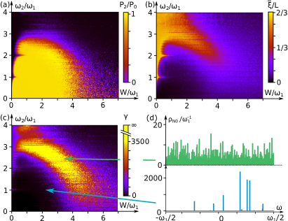
Figure 2: Simulation of the QFTEP with $200$ unit cells and open boundary conditions, as detailed in the numerics section. (a) Average energy absorption rate over $10\hskip 1.5pt000$ periods of mode $1$ when the left half of the chain is initially occupied. (b) Estimated spatial localization length of the generalized Floquet states, $\xi$. (c) Effective spectral density of the system, $\gamma$. (d) Spectral density $\rho_{N_{0}}(\omega)$ resulting from a wave-packet initialized on a single site in the middle of the chain for parameters within the topological plateau (bottom), and at the transition (top).

Numerical simulations — We demonstrate the quantized energy pumping of the QFTEP through numerical simulations of the model presented in the introduction. We simulated a system of $L=200$ unit cells ($400$ sites) with open boundary conditions, initialized by only filling the leftmost 200 sites with fermions. Using direct time evolution, we computed the time-averaged rate of energy transfer to mode $2$, $\bar{\mathcal{P}}_{2}$, by averaging $\langle\hat{\mathcal{P}}_{2}(t)\rangle$ over the time-interval from $0$ to $t_{\rm f}=10,\!000\,T_{1}$. Fig. 2(a) shows $\bar{\mathcal{P}}_{2}/\mathcal{P}_{0}$, as a function of $\omega_{2}$ and $W$ ome . The data indicate a large plateau of quantized energy pumping ($\bar{\mathcal{P}}_{2}=\mathcal{P}_{0}$) at finite values of $\omega_{2}$ and $W$, supporting our conclusions above.

The data in Fig. 2(a) exhibit several features that are consistent with our discussion above. The plateau with $\bar{\mathcal{P}}_{2}=\mathcal{P}_{0}$ has maximal extent along the $\omega_{2}$-direction when $W\approx\omega_{1}$, indicating that weak to moderate disorder stabilizes the QFTEP (interestingly, for $\omega_{2}\ll\omega_{1}$, stabilization occurs for very weak disorder). The quantized plateau diminishes when $\omega_{2}/\omega_{1}$ approaches values $p/q$ for integers $p$ and $q$, as is particularly clear for $q=1$, where the yellow plateau region is sharply “pinched in.” In the SOM we provide high-resolution data confirming that quantization of $\bar{\mathcal{P}}_{2}$ breaks down for other values of $p$ and $q$, with the breakdown most pronounced for smaller $p$ and $q$. These data thus support our prediction that the QFTEP is protected by the irrationality of $\omega_{2}/\omega_{1}$.

To characterize the phase transitions of the QFTEP, we estimate the spatial localization length of the generalized Floquet states in the system via $\xi\equiv\sup_{x_{1}}\ (\sum_{x_{2}}|\langle x_{1}|\hat{U}(t_{\rm f})|x_{2}\rangle|^{2}(x_{1}-x_{2})^{2})^{1/2}$. Fig. 2(b) shows $\xi$ for the same parameters as taken in Fig. 2(a). For $W\lesssim 4\omega_{1}$, the boundary of the topological plateau in Fig. 2(a) clearly coincides with the region in Fig. 2(b) where $\xi\sim\mathcal{O}(L)$ (indicating delocalization). For $\omega_{2},W\gtrsim 3\omega_{1}$ we observe a localized, topologically-trivial phase with $\xi\sim\mathcal{O}(1)$ and $\bar{\mathcal{P}}_{2}=0$ [Figs. 2(a-b)]. Rather than a direct transition to this topologically trivial phase, Fig. 2(b) indicates the existence of an intermediate delocalized region for $W\lesssim 3\omega_{1}$, $\omega_{2}\gtrsim 3\omega_{1}$.

When $W$ exceeds $3\,\omega_{1}$, the topological phase transition changes its qualitative behavior: $\xi$ decreases and $\bar{\mathcal{P}}_{2}$ displays irregular fluctuations for a finite $\omega_{2}$-interval. To investigate the transition here, we computed a measure of the frequency-space localization length, using the time-evolution of a single-particle state initialized on a particular site $x_{\rm i}$ in the chain, $|\psi(t)\rangle\equiv\hat{U}(t)|x_{\rm i}\rangle$. For a given (large) integer $N$, we let $|\psi_{N}(\omega)\rangle\equiv\frac{1}{\sqrt{\omega_{1}N}}\sum_{n=1}^{N}e^{in\omega T_{1}}|\psi(n{T_{1}})\rangle$ denote the finite-time discrete Fourier transform of $|\psi(t)\rangle$ when sampled stroboscopically with the period of mode 1. We then define an effective spectral density $\gamma$ characterizing $|\psi(t)\rangle$ via the inverse participation ratio of the normalized spectral distribution $\rho_{N}(\omega)\equiv|\langle\psi_{N}(\omega)|\psi_{N}(\omega)\rangle|$: $\gamma\equiv\frac{1}{\omega_{1}}\lim_{N\to\infty}N/[\int_{0}^{\omega_{1}}\!\!{\rm d\omega}\rho_{N}(\omega)^{2}]$. When $|\psi(t)\rangle$ has a dense Fourier spectrum, $\int_{0}^{\omega_{1}}\!\!{\rm d\omega}\rho_{N}(\omega)^{2}$ remains finite in the limit $N\to\infty$, and thus $\gamma$ diverges. However, for a discrete spectrum, where $\rho_{\infty}(\omega)\equiv\lim_{N\to\infty}\rho_{N}(\omega)$ is given by a discrete sum of delta functions, the integral diverges linearly with $N$, such that $\gamma$ remains finite. In this case, $\gamma$ gives the inverse sum of the squared peak weights in $\rho_{\infty}(\omega)$; i.e., it measures effective number of peaks in the frequency spectrum of $|\psi(t)\rangle$ (modulo $\omega_{1}$), $\rho_{\infty}(\omega)$. We hence expect that $\gamma$ is a good proxy for the localization length in the frequency space of mode $2$.

Fig. 2(c) shows the maximal value of $\gamma$ obtained from $15$ time-evolved single-particle states with initial positions $x_{\rm i}$ randomly chosen within the middle third of the system. We used the same parameters as considered in panels (a-b), and set $N$ to $N_{0}=10\hskip 1.5pt000$. As an illustration, in Fig. 2(d), we plot $\rho_{N_{0}}(\omega)$ for two parameter sets [indicated with arrows in Fig. 2(c)] where $\gamma$ is large (upper) and small (lower), respectively. Although Fig. 2(b) does not conclusively indicate whether spatial delocalization is present for $W\gtrsim 3\omega_{1}$, Fig. 2(c) shows that the system undergoes frequency delocalization throughout the entire topological phase boundary.

Realization in a driven two-level system — Here we propose a dimensionally-reduced experimental realization of the QFTEP in a two-level system (qubit) driven by three incommensurate modes. The model presented in the introduction is mapped to this platform by taking the limit of zero disorder, and replacing spatial crystal momentum with the phase of a third driving mode: $e^{ik}\to e^{i\omega_{3}t}$ Qi et al. (2008). When the frequencies $\omega_{1},\omega_{2}$, and $\omega_{3}$ are sufficiently incommensurate, the generalized Floquet eigenstates of the system remain localized due to the quasi-disorder of the lattice in the three-dimensional frequency space Ho et al. (1983); Luck et al. (1988); Casati et al. (1989); Blekher et al. (1992); Hatami et al. (2016); Else et al. (2020); SOM . The analysis below Eq. (1) thereby also yields the topological index $\nu$ for this model, defined by Eq. (2) with $\theta$ replaced by the phase $\phi_{3}=\omega_{3}t$ of the third driving field. In the SOM we provide data from numerical simulations that confirm the 3-mode driven qubit model described above supports a topologically nontrivial regime characterized by $\nu=1$. Edges can naturally be incorporated into the qubit realization by replacing one or more of the driving modes by quantized cavity modes, whose vacuum states define a natural edge.

Summary and outlook — This work establishes the QFTEP as a new non-equilibrium topological phase. The QFTEP elevates the Floquet-Thouless energy pump (FTEP) in Ref. Kolodrubetz et al. (2018) from a fine-tuned (but nonetheless interesting) phenomenon to a genuine stable phase of matter. Whereas the FTEP requires adiabatic driving, fine-tuning, and is formally destroyed by disorder Kolodrubetz et al. (2018), the QFTEP arises for finite $\omega_{1}$ and $\omega_{2}$, and is stabilized by disorder.  In a setting with open boundary conditions, the QFTEP is characterized by robust, quantized energy pumping between the two driving modes, supported by topological edge states.

We showed that a qubit driven by three incommensurate modes can realize a dimensionally-reduced version of the QFTEP. Such a system is a promising platform for experimental realization of this phenomenon due to well-developed techniques for controlling and driving qubits Vahala (2003). The QFTEP may also be directly realized in one-dimensional quantum chains, such as systems of ultracold atoms in optical lattices, or trapped-ion systems. The robustness to disorder and finite modulation frequency makes such realizations of the QFTEP more feasible than for the adiabatic FTEP.

Quantization of energy pumping breaks down for rational values of $\omega_{1}/\omega_{2}$, implying that the phase diagram of the QFTEP has a fractal structure. Understanding this fractal structure and its role for the phase transitions of the QFTEP will be an interesting direction for future studies.

Another prospect for invesigations is to apply our dimensional reduction scheme to other equilibrium or Floquet topological phases of matter. A more complete investigation of the physical signatures of the QFTEP, its stability to interactions, and its place in the expanding classification of non-equilibrium topological phases of matter will also be important future directions.

Acknowledgements — We thank Anushya Chandran, Philip Crowley, David Long, Ivar Martin, and Gil Refael for valuable discussions. This work was performed with support from the National Science Foundation through award number DMR-1945529 and the Welch Foundation through award number AT-2036-20200401 (M.K. and R.G.). S.G. acknowledges support from the Israel Science Foundation, Grant No. 1686/18. F.N. and M.R. gratefully acknowledge the support of the European Research Council (ERC) under the European Union Horizon 2020 Research and Innovation Programme (Grant Agreement No. 678862), and the Villum Foundation. We used the computational resources of the Lonestar 5 cluster operated by the Texas Advanced Computing Center at the University of Texas at Austin and the Ganymede and Topo clusters operated by the University of Texas at Dallas’ Cyberinfrastructure & Research Services Department.

Note added by the authors — During the preparation of this manuscript, a preprint appeared which describes an energy pumping phenomenon related to the one we consider here Long et al. (2021), in the context of a general classification. Our work is fully consistent with Ref. Long et al. (2021), and provides a complementary perspective on the phenomenon, including a study of the role of spatial disorder, along with additional experimental proposals for realizing the phase.

I Extended Hilbert space and frequency localization

In this section, we provide details of the extended Hilbert space approach that was used in the main text (See also, e.g., Refs. Ho et al. (1983); Luck et al. (1988); Casati et al. (1989); Blekher et al. (1992); Hatami et al. (2016); Else et al. (2020)). In Sec. I.1 we define the extended Hilbert space Hamiltonian that results from including the Fourier harmonic (or “frequency”) space of mode $2$, $\hat{\bm{H}}_{\rm 2d}(t)$, and show how the generalized Floquet states of $\hat{H}(t)$ can be obtained from the Floquet states of $\hat{\bm{H}}_{\rm 2d}(t)$. We subsequently demonstrate how frequency localization is equivalent to spatial localization of the Floquet states of $\hat{\bm{H}}_{\rm 2d}(t)$ (Sec. I.2).

I.1 Extended Hilbert space

As explained in the main text, the generalized Floquet states of $\hat{H}(t)$, $\{|\Phi_{n}(\phi_{1},\phi_{2})\rangle\}$, can be obtained from the Floquet states of a periodically driven, two-dimensional system with Hamiltonian $\hat{\bm{H}}_{\rm 2d}(t)$ Ho et al. (1983); Luck et al. (1988); Casati et al. (1989); Blekher et al. (1992); Hatami et al. (2016); Else et al. (2020). The extra dimension in this “extended space” corresponds to the Fourier harmonic index ($q$) in the Fourier decomposition of $|\Phi_{n}(\omega_{1}t,\omega_{2}t)\rangle$ with respect to mode $2$:

$$|\Phi_{n}(\phi_{1},\phi_{2})\rangle=\sum_{q}e^{iq\phi_{2}}|\Phi_{n}^{(q)}(\phi_{1})\rangle.$$ (4)

To construct $\hat{\bm{H}}_{2{\rm d}}(t)$ we introduce an effective position operator $\hat{n}_{2}$ in the Fourier harmonic space of mode $2$; as explained in the main text, this operator can heuristically be seen as counting the number of photons in mode $2$ Shirley (1965). The energy in mode $2$ transforms to an effective linear potential along the corresponding lattice direction, $\omega_{2}\hat{n}_{2}$, and each factor of $e^{-im\omega_{2}t}$ in $\hat{H}(t)$ induces an $m$-th neighbor hopping term in the corresponding direction, $e^{-i\omega_{2}mt}\to\hat{B}^{(m)}_{2}=\sum_{y=-\infty}^{\infty}|y\rangle\langle y+m|$, where $\hat{n}_{2}|y\rangle=y|y\rangle$. Applying this transformation thus yields:

$$\hat{\bm{H}}_{2{\rm d}}(t)=\omega_{2}\hat{n}_{2}+\sum_{q}\hat{H}^{(q)}(t)\hat{B}_{2}^{(q)},$$ (5)

where $\hat{H}^{(q)}(t)$ denotes the $q$-th Fourier component of the single-particle Hamiltonian with respect to the phase of mode $2$, $\hat{H}^{(q)}(t)\equiv\frac{1}{2\pi}\int_{0}^{2\pi}\!\!{\rm d}\phi_{2}\,\tilde{H}(\omega_{1}t,\phi_{2})e^{iq\phi_{2}}$, where $\tilde{H}(\phi_{1},\phi_{2})$ denotes the single-particle Hamiltonian of the system as a function of the two modes’ phases (i.e., the restriction of $\tilde{\mathcal{H}}(\phi_{1},\phi_{2})$ the single-particle sector). In the following we use double brackets, $|\cdot\rangle\!\rangle$, for states that live in the extended Hilbert space on which $\hat{\bm{H}}_{\rm 2d}(t)$ acts.

The Hamiltonian $\hat{\bm{H}}_{\rm 2d}(t)$ describes a two-dimensional single-particle system, where the $x$-direction corresponds to the original (spatial) coordinate, and the $y$-direction to the Fourier harmonic index $n_{2}$. Evidently, $\hat{\bm{H}}_{\rm 2d}(t)$ has periodic time-dependence with the period of mode $1$, $T_{1}$: $\hat{\bm{H}}_{\rm 2d}(t)=\hat{\bm{H}}_{\rm 2d}(t+T_{1})$. As a result, the time-evolution generated by $\hat{\bm{H}}_{\rm 2d}(t)$ can be decomposed in terms of a complete orthonormal basis of Floquet states $\{|\Psi_{n}(t)\rangle\!\rangle\}$ that are time-periodic with period $T_{1}$: $|\Psi_{n}(t)\rangle\!\rangle=|\Psi_{n}(t+T_{1})\rangle\!\rangle$ Shirley (1965). For any Floquet state of $\hat{\bm{H}}_{\rm 2d}(t)$, $|\Psi_{n}(t)\rangle\!\rangle$, it is possible to identify a unique generalized Floquet state of $\hat{H}(t)$, $|\Phi_{n^{\prime}}(\phi_{1},\phi_{2})\rangle$ such that, for any state $|\alpha\rangle$ in the 1d system:

$$\langle\alpha|\Phi^{(q)}_{n^{\prime}}(\omega_{1}t)\rangle=\langle\!\langle\alpha,q|\Psi_{n}(t)\rangle\!\rangle,$$ (6)

where $|\alpha,n_{2}\rangle\!\rangle\equiv|\alpha\rangle\otimes|n_{2}\rangle$ denotes the basis state in the extended Hilbert space at location $y=n_{2}$ corresponding to $|\alpha\rangle$ Ho et al. (1983); Luck et al. (1988); Casati et al. (1989); Blekher et al. (1992); Hatami et al. (2016); Else et al. (2020). This establishes the relationship between the Floquet states of $\hat{\bm{H}}_{\rm 2d}(t)$ and the generalized Floquet states of $\hat{H}(t)$.

Due to the built-in symmetry of $\hat{\bm{H}}_{\rm 2d}(t)$, $\hat{B}^{(1)}_{2}\hat{\bm{H}}_{\rm 2d}(t)[\hat{B}^{(1)}_{2}]^{\dagger}=\hat{\bm{H}}_{\rm 2d}+\omega_{2}$, the Floquet states of $\hat{\bm{H}}_{\rm 2d}(t)$ can be grouped into families whose elements are mapped to each other through shifts in $n_{2}$: if $|\Psi_{n}(t)\rangle\!\rangle$ is a Floquet state of $\hat{\bm{H}}_{\rm 2d}(t)$ with associated quasienergy $\varepsilon_{n}$, for each $m$, $\hat{B}_{2}^{(m)}|\Psi_{n}(t)\rangle\!\rangle$ also is a Floquet state of $\hat{\bm{H}}_{\rm 2d}(t)$, with quasienergy $\varepsilon_{n}-m\omega_{2}$. Through Eq. (6) each such family of Floquet states of $\hat{\bm{H}}_{\rm 2d}(t)$ correspond to the same generalized Floquet state of $\hat{H}(t)$, up to a $\phi_{1}$-dependent phase factor.

The above mapping can be also applied to mode $1$. In particular, the operation that maps $\hat{H}(t)$ to $\hat{\bm{H}}_{\rm 2d}(t)$ in Eq. (5) can subsequently be applied to the latter, resulting a time-independent Hamiltonian of a 3-dimensional system, where the third dimension corresponds to the Fourier harmonic index with respect to mode $1$ Shirley (1965). The same approach can moreover be generalized to systems driven quasiperiodically by $3$ or more modes Ho et al. (1983); Luck et al. (1988); Casati et al. (1989); Blekher et al. (1992); Hatami et al. (2016); Else et al. (2020).

I.2 Frequency localization

We now show that frequency localization of $\hat{H}(t)$ is equivalent to spatial localization of the Floquet states of $\hat{\bm{H}}_{\rm 2d}(t)$.

As described in the main text, frequency localization arises when each generalized Floquet state of $\hat{H}(t)$, $|\Phi_{n}(\phi_{1},\phi_{2})\rangle$, is continuous in its arguments $\phi_{1}$ and $\phi_{2}$. Such continuity occurs when $|\Phi_{n}(\phi_{1},\phi_{2})\rangle$ can be approximated arbitrarily well by truncating its Fourier decomposition,

$$|\Phi_{n}(\phi_{1},\phi_{2})\rangle=\sum_{p,q}e^{ip\phi_{1}+iq\phi_{2}}|\Phi_{n}^{(p,q)}\rangle,$$ (7)

at some sufficiently large, but finite, cutoff in the Fourier Harmonic indices $p$ and $q$. Note that the boundedness of $\hat{H}(t)$ [and hence also $\partial_{t}U(t)$], along with Eq. (1) of the main text, implies that, as a function of $p$ and $q$, $|\Phi_{n}^{(p,q)}\rangle$ may can only be significant near a particular line where $p\omega_{1}+q\omega_{2}$ takes some (given) constant value. Consequently, frequency localization is ensured when $|\Phi_{n}^{(p,q)}\rangle$ effectively only has significant support for a finite range of $q$. To be more precise, frequency localization occurs when the squared norm of $|\Phi_{n}^{(p,q)}\rangle$ for large $q$ falls off at least as fast as $|q|^{-\alpha}$ for some $\alpha>1$. (The condition can equivalently be expressed in terms of $p$.) In this sense, frequency localization with respect to mode $2$ implies frequency localization with respect to mode $1$, and vice versa.

To relate frequency localization to the localization properties of $\hat{\bm{H}}_{\rm 2d}(t)$, we note from Eq. (6) that

$$\langle\alpha|\Phi^{(p,q)}_{n^{\prime}}\rangle=\frac{1}{T_{1}}\int_{0}^{T_{1}}\!\!{\rm dt}e^{-i\omega_{1}t}\langle\!\langle\alpha,q|\Psi_{n}(t)\rangle\!\rangle.$$ (8)

From the discussion above, we conclude that frequency localization arises when the Floquet states of $\hat{\bm{H}}_{\rm 2d}(t)$, $\{|\Psi_{n}(t)\rangle\!\rangle\}$, are spatially localized in the $y$-direction (corresponding to the Fourier Harmonic index of mode $2$, $q$).

We expect frequency localization automatically implies full localization (i.e., localization of the generalized Floquet states of $\hat{H}(t)$ both in real and frequency space): for a frequency localized system, we expect the Floquet states of $\hat{\bm{H}}_{\rm 2d}(t)$ can be obtained to arbitrarily high precision by truncating the extended Hilbert space at some sufficiently large cutoff in $n_{2}$. Since the resulting system is effectively one-dimensional, the Floquet states of $\hat{\bm{H}}_{\rm 2d}(t)$ are subject to Anderson localization Shirley (1965), and hence will also be spatially localized.

II Role of incommensurability

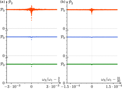
Figure 3: Breakdown of quantization of energy pumping near rational frequency ratios. Left and right panels show the average rate of energy transfer to mode $2$, $\bar{\mathcal{P}}_{2}$, in a QFTEP model with disorder strength $W=2\omega_{1}$, computed for different values of $\omega_{2}$ in the vicinity of $\frac{3}{2}\omega_{1}$ (a) and $\frac{31}{20}\omega_{1}$ (b). For each probed value of $\omega_{2}$, $\bar{\mathcal{P}}_{2}$ is computed for several disorder realizations and values of the initial phase difference between the driving modes, $\Delta\phi$. Red data points (top) show the values of $\bar{\mathcal{P}}_{2}$ obtained from individual disorder realizations with randomly chosen $\Delta\phi$, blue data points (middle) show the value of $\bar{\mathcal{P}}_{2}$ after averaging over $\sim 10$ disorder realizations with $\Delta\phi=0$, and green data points (bottom) show the value of $\bar{\mathcal{P}}_{2}$ after averaging over $\sim 80$ disorder realizations with randomly chosen $\Delta\phi$. See main text for further details of the model and simulation. Note the different scales on the $x$-axes in panels (a) and (b).

Here we provide additional details of the relationship between frequency localization and the incommensurability of $\omega_{1}$ and $\omega_{2}$. We moreover provide data from numerical simulations to demonstrate that the quantization of the energy pumping rate, $\bar{\mathcal{P}}_{2}$, breaks down near rational values of $\omega_{2}/\omega_{1}$.

The condition of irrationality of $\omega_{2}/\omega_{1}$ can be understood from the extended Hilbert space picture: when $\omega_{2}/\omega_{1}$ is sufficiently close to $p/q$ for some integers $p$ and $q$, the oscillating terms of ${\bm{H}}_{\rm 2d}(t)$ resonantly couple sites separated by $q$ lattice constants in the $y$-direction, inducing $y$-delocalization, and hence frequency delocalization Blekher et al. (1992); Else et al. (2020). For each pair of integer values of $p$ and $q$, frequency localization hence breaks down in some finite $\omega_{2}$-interval around $\omega_{2}=p\omega_{1}/q$, $I_{pq}$.

We expect that the width of $I_{pq}$, $|I_{pq}|$, decays as a function of $p$ and $q$, with a rate controlled by the harmonic structure of $\tilde{H}(\phi_{1},\phi_{2})$. Specifically, if the $(p,q)$th Fourier coefficient of $\tilde{H}(\phi_{1},\phi_{2})$, $\tilde{H}_{pq}$, is nonzero, sites in the 2d lattice separated by $(p,q)$ lattice constants are coupled directly by $\hat{\bm{H}}_{\rm 2d}(t)$, and we expect $|I_{pq}|$ to scale with $|\tilde{H}_{pq}|$. If on the other hand the Fourier coefficient $\tilde{H}_{mn}$ is only significant for a few small values of $m$ and $n$ (i.e., if the $\tilde{H}(\phi_{1},\phi_{2})$ is a smooth function of its arguments), the resonant coupling for large $p,q$ is induced by high-order virtual processes. In this case we expect $|I_{pq}|$ to decrease exponentially as a function of $p$ and $q$.

The decay of $|I_{pq}|$ with $p$ and $q$ means that frequency localization can occur for a finite-measure set of $\omega_{2}$ even though it breaks down for a dense set of points. Additionally, it is more likely to occur for highly irrational values of $\omega_{2}/\omega_{1}$, i.e., when $\omega_{2}/\omega_{1}$ is not close to $p/q$ for some small integers $p$ and $q$ .

To support the discussion above, we simulated the QFTEP model introduced in the main text [see Fig. 1(c)] for values of $\omega_{2}$ near rational multiples of $\omega_{1}$. We chose the disorder strength $W=2\omega_{1}$, which places the system within the $\nu=1$ QFTEP phase for $0<\omega_{2}\lesssim 2.5\omega_{1}$ [see Fig. 2(a) in the main text]. For values of $\omega_{2}$ which we specify below, we computed the average rate of energy transfer to mode $2$, $\bar{\mathcal{P}}_{2}$, over a time-interval of length $10\,000\,T_{1}$, after initializing the system with the leftmost $200$ sites occupied by fermions and the remaining sites empty (i.e., we performed the same calculation as used for Fig. 2 in the main text).

For each value of $\omega_{2}$ we probed, we computed $\bar{\mathcal{P}}_{2}$ for multiple disorder realizations, and for multiple values of the initial phase difference between the two modes, $\Delta\phi$. Here $\Delta\phi$ controls the offset of the second argument of $\tilde{\mathcal{H}}$, such that the Hamiltonian of the system in our simulation is given by $\hat{\mathcal{H}}(t)=\tilde{\mathcal{H}}(\omega_{1}t,\omega_{2}t+\Delta\phi)$ (see main text for definition of $\hat{\mathcal{H}}$ and $\tilde{\mathcal{H}}$). For incommensurate frequencies, different values of $\Delta\phi$ correspond to shifts of time-origin, and thus lead to the same value of $\bar{\mathcal{P}}_{2}$ after averaging over sufficiently long time intervals. For commensurate or near-commensurate frequencies (i.e., frequencies that are effectively commensurate over the time-window we probe), $\bar{\mathcal{P}}_{2}$ generally depends on $\Delta\phi$, which is why we introduce this parameter in our simulations.

We first computed $\bar{\mathcal{P}}_{2}$ for $\omega_{2}/\omega_{1}$ near the rational value $3/2$. The corresponding data are plotted in Fig. 3(a). For each value of $\omega_{2}$ probed in Fig. 3(a), we computed $\bar{\mathcal{P}}_{2}$ for $\sim 80$ different disorder realizations and randomly selected values of $\Delta\phi$, with each value shown as a separate data point in red. For most probed $\omega_{2}$-values, $\bar{\mathcal{P}}_{2}$ takes the quantized value $\mathcal{P}_{0}$ for all disorder realizations. However, when $\omega_{2}/\omega_{1}$ approaches $3/2$, the quantization clearly breaks down. We estimate the $\omega_{2}$-interval where the quantization of $\bar{\mathcal{P}}_{2}$ breaks down for individual realizations to have width of order $5*10^{-4}\omega_{1}$. The breakdown of quantization persists after averaging $\bar{\mathcal{P}}_{2}$ over individual disorder realizations with the value of $\Delta\phi$ fixed to zero (blue data points), or averaging over disorder realizations and values of $\Delta\phi$ (green). The data thus agree well with our expectation that the quantization of $\bar{\mathcal{P}}_{2}$ breaks down near rational values of $\omega_{2}/\omega_{1}$.

Next, we computed $\bar{\mathcal{P}}_{2}$ for $\omega_{2}/\omega_{1}$ near the “less rational” value $31/20$, using the same method as above. The corresponding data are plotted in Fig. 3(b) [note that the $x$ axis is rescaled by a factor $20$ relative to the $x$-axis in Fig. 3(a)]. As Fig. 3(b) shows, $\bar{\mathcal{P}}_{2}$ clearly deviates from the quantized value $\mathcal{P}_{0}$ when $\omega_{2}/\omega_{1}$ approaches $31/20$. However, the deviation from quantization is not as pronounced as in panel (a), and the breakdown occurs in a much smaller interval of $\omega_{2}$. We estimate the the $\omega_{2}$-interval where quantization breaks down for individual realizations to have width of order $10^{-5}\omega_{1}$, and thus be a factor $\sim 50$ smaller than the corresponding interval surrounding $\omega_{2}=\frac{3}{2}\omega_{1}$. These features thus agree with our expectation that the breakdown of quantization of $\bar{\mathcal{P}}_{2}$ near rational frequency ratios $\omega_{2}/\omega_{1}=p/q$ is more pronounced at highly rational frequency ratios (i.e., for small $p$ and $q$) than at less rational frequency ratios (i.e., for large $p$ and $q$).

III Unitarity of $\hat{P}_{\theta}(\phi_{1},\phi_{2})$

Here we show that “phase-twisted” micromotion operator $\hat{P}_{\theta}(\phi_{1},\phi_{2})$ [introduced above Eq. (2) in the main text] is unitary when the generalized Floquet states of the system are spatially localized on the scale of the system size, $L$. We used this result in the main text to establish the integer quantization of the invariant $\nu$ that characterizes the QFTEP.

We recall that $\hat{P}_{\theta}(\phi_{1},\phi_{2})$ is constructed from the generalized micromotion operator in Eq. (1) by appending the phase factor $e^{-i\theta}$ ($e^{i\theta}$) to matrix elements of $\hat{P}(\phi_{1},\phi_{2})$ that hop a particle across a cut at $x=x_{0}+1/2$ in the positive (negative) $x$-direction, where $x_{0}$ is some arbitrary reference site. In the case of periodic boundary conditions, the hopping trajectory between two sites is defined to be the shortest path between the sites on the lattice. Thus, letting $|\alpha\rangle$ denote the single-particle state where the particle is located on site $\alpha$, $\hat{P}_{\theta}(\phi_{1},\phi_{2})$ can be written:

$$\hat{P}_{\theta}(\phi_{1},\phi_{2})=\sum_{\alpha,\beta}|\alpha\rangle\langle\alpha|\hat{P}(\phi_{1},\phi_{2})|\beta\rangle\langle\beta|e^{-is_{\alpha\beta}\theta},$$ (9)

where $s_{\alpha\beta}$ takes value $1$ ($-1$) if the shortest path from site $\alpha$ to site $\beta$ traverses the cut at $x=x_{0}+1/2$ in the positive (negative) $x$-direction, and takes value $0$ if the path does not traverse this cut. In particular, $s_{\alpha\alpha}=0$. In the case of periodic boundary conditions (when the generalized Floquet states are localized on the scale $L$), the operation above is equivalent to inserting a flux $\theta$ through the closed chain formed by the system, with a gauge where the corresponding phases are applied locally Titum et al. (2016).

To establish the unitarity of $\hat{P}_{\theta}$ we first note that

$$\langle\alpha_{1}|\hat{P}_{\theta}^{\dagger}\hat{P}_{\theta}|\alpha_{2}\rangle=\sum_{\beta}\langle\alpha_{1}|\hat{P}^{\dagger}|\beta\rangle\langle\beta|\hat{P}|\alpha_{2}\rangle e^{-i\theta(s_{\alpha_{1}\beta}-s_{\alpha_{2}\beta})},$$ (10)

where, here and below, we suppress the dependence of $\hat{P}_{\theta}(\phi_{1},\phi_{2})$ and $\hat{P}(\phi_{1},\phi_{2})$ on $\phi_{1},\phi_{2}$ for brevity.

From the definition of $\hat{P}$ below Eq. (1) in the main text, we see that $\langle\alpha|\hat{P}|\beta\rangle$ is only nonzero when sites $\alpha$ and $\beta$ are located within a distance of order $\xi$ from each other, where $\xi$ denotes the spatial localization length of the generalized Floquet states. Using our assumption that $\xi$ is much smaller than the system size, $L$, one can confirm that $s_{\alpha_{1}\beta}-s_{\alpha_{2}\beta}=s_{\alpha_{1}\alpha_{2}}$ for all contributing terms in the sum in Eq. (10). Using this in Eq. (10), we obtain

$$\langle\alpha_{1}|\hat{P}_{\theta}^{\dagger}\hat{P}_{\theta}|\alpha_{2}\rangle=\langle\alpha_{1}|\hat{P}^{\dagger}\hat{P}|\alpha_{2}\rangle e^{-i\theta s_{\alpha_{1}\alpha_{2}}}.$$ (11)

Since $\hat{P}$ is unitary, $\langle\alpha_{1}|P^{\dagger}P|\alpha_{2}\rangle=\delta_{\alpha_{1}\alpha_{2}}$, where $\delta_{ab}$ denotes the Kronecker symbol. Using that $s_{\alpha\alpha}=0$, we find $\langle\alpha_{1}|\hat{P}_{\theta}^{\dagger}\hat{P}_{\theta}^{\dagger}|\alpha_{2}\rangle=\delta_{\alpha_{1}\alpha_{2}}$. Thus we conclude that $\hat{P}_{\theta}$ is unitary, which was the goal of this section.

IV Relationship with AFAI

Here we show that the q-FTEP invariant $\nu$ is identical to the AFAI invariant of the extended Hilbert space Hamiltonian of the system, $\hat{\bm{H}}_{\rm 2d}(t)$, which was introduced below Eq. (1) in the main text Titum et al. (2016). To be more specific, recall from the main text $\nu$ is robustly quantized when the generalized Floquet states of $\hat{H}(t)$ are localized both in position and frequency space. Such full localization is equivalent to spatial localization of the Floquet states of $\bm{\hat{H}}_{\rm 2d}(t)$. When such localization occurs, $\bm{\hat{H}}_{\rm 2d}(t)$ is characterized by the integer-valued winding number of the AFAI, $\nu_{\rm AFAI}$, Titum et al. (2016); bou . The goal of this section is to show that $\nu=\nu_{\rm AFAI}$.

To establish that $\nu=\nu_{\rm AFAI}$, we note that the latter can be defined from an analogous expression to Eq. (2) from the main text using the $T_{1}$-periodic micromotion operator of $\hat{\bm{H}}_{\rm 2d}(t)$, $\bm{\hat{P}}(t)\equiv\sum_{n}|\Psi_{n}(t)\rangle\!\rangle\langle\!\langle\Psi_{n}(0)|,$ where $\{|\Psi_{n}(t)\rangle\!\rangle\}$ denote the Floquet states of $\hat{\bm{H}}_{\rm 2d}(t)$ (see Sec. I). Analogously to the “phase-twisted” micromotion operator $\hat{P}_{\theta}(\phi_{1},\phi_{2})$ from the main text, we construct the phase-twisted micromotion operator $\bm{\hat{P}}_{\theta_{1},\theta_{2}}(t)$ by appending the phase factor $e^{-i\theta_{x}}$ ($e^{i\theta_{x}}$) to matrix elements of $\bm{\hat{P}}(t)$ that hop a particle across a cut at $x=x_{0}+1/2$ in the positive (negative) $x$-direction, and similarly assign $e^{\mp i\theta_{y}}$ to the matrix elements that hop across a cut at $y=y_{0}+1/2$, for some arbitrary reference sites $x_{0}$ and $y_{0}$. From $\bm{\hat{P}}_{\theta_{1},\theta_{2}}(t)$, we can compute $\nu_{\rm AFAI}$ as follows Martin et al. (2017):

$$\nu_{\rm AFAI}=\!\oint\!\frac{{\rm d}^{2}\theta{\rm d}t}{8\pi^{2}}{\rm Tr}\Big{(}\!\bm{\hat{P}}^{-1}\partial_{t}{\bm{\hat{P}}}\,[\bm{\hat{P}}^{-1}\partial_{\theta_{1}}\bm{\hat{P}}\,,\,\bm{\hat{P}}^{-1}\partial_{\theta_{2}}\bm{\hat{P}}]\Big{)},$$ (12)

where we suppressed the dependence of $\bm{\hat{P}}_{\theta_{1},\theta_{2}}(t)$ on $\theta_{1},\theta_{2}$, and $t$ in the above for brevity. Through the correspondence between the generalized Floquet states of $\hat{H}(t)$ and the Floquet states of ${\hat{\bm{H}}}_{\rm 2d}(t)$ in Eq. (6), it can be shown by direct insertion that $\nu_{\rm AFAI}$ is identical to $\nu$, as defined in Eq. (2) of the main text.

V Bulk-edge correspondence

Here we establish Eq. (3) in the main tex, which gives the bulk-edge correspondence for the quasiperiodic Floquet-Thouless energy pump: we show that in a setting with open boundary conditions, when the system is initialized by filling all sites from the left end up to a given (arbitrary) site located well within the bulk, $x_{1}$, the average rate of energy transfer from the system to mode $2$ is given by $\nu\mathcal{P}_{0}$, where $\mathcal{P}_{0}=2\pi\omega_{1}\omega_{2}$ denotes the “quantum of energy transfer.” Specifically, we show that

$$\lim_{\tau\to\infty}\frac{1}{\tau}\int_{0}^{\tau}\!\!{\rm d}t\,\langle\hat{\mathcal{P}}_{2}(t)\rangle=\nu\mathcal{P}_{0},$$ (13)

where, as in the main text, the many-body operator $\hat{\mathcal{P}}_{2}(t)$ denotes the rate of energy transfer to mode $2$ from the system: $\hat{\mathcal{P}}_{2}(t)\equiv-\omega_{2}\partial_{\phi_{2}}\tilde{\mathcal{H}}(\omega_{1}t,\omega_{2}t)$, where $\tilde{\mathcal{H}}(\phi_{1},\phi_{2})$ denotes the many-body Hamiltonian of the system as a function of the phases of the two modes (see also main text).

To obtain Eq. (13), we recall that time-evolved many-body states in the system are given by Slater determinants of time-evolved single-particle states (due to the absence of interactions). Hence the evolution resulting from the initialization above can be decomposed in terms of the evolved single-particle states $\{|\psi_{x}(t)\rangle\}$, $x=1\ldots x_{1}$, where $|\psi_{x}(t)\rangle$ describes the evolution resulting from initializing the system with a single fermion on site $x$. In particular,

$$\langle\hat{\mathcal{P}}_{2}(t)\rangle=\sum_{x=1}^{x_{1}}\omega_{2}F_{2,x}(t),$$ (14)

where $F_{2,x}=-\langle\psi_{x}(t)|\partial_{\phi_{2}}\tilde{H}(\omega_{1}t,\omega_{2}t)|\psi_{x}(t)\rangle$ denotes the generalized force exerted on mode $2$ by the system in the state $|\psi_{x}(t)\rangle$, and $\tilde{H}(\phi_{1},\phi_{2})$ denotes the single-particle Hamiltonian as a function of the two modes’ phases (i.e., the restriction of $\tilde{\mathcal{H}}(\phi_{1},\phi_{2})$ to the single-particle sector).

Through the correspondence between the generalized Floquet eigenstates of $\hat{H}(t)$ and the Floquet states of $\hat{\bm{H}}_{\rm 2d}(t)$ in Eq. (6), one can verify that the long-time-averaged value of $F_{2,x}(t)$, $\bar{F}_{2,x}\equiv\lim_{\tau\to\infty}\frac{1}{\tau}\int_{0}^{\tau}\!{\rm d}t\,F_{2,x}(t)$, gives the time-averaged $y$-velocity, $\bar{v}_{y}(x,0)$ of a particle initially localized on the site $(x,0)$ in the two-dimensional system described by $\hat{\bm{H}}_{\rm 2d}(t)$. From the built-in symmetry of $\hat{\bm{H}}_{\rm 2d}(t)$ (see Sec. I.1) one can moreover verify that $\sum_{x=1}^{x_{1}}\bar{v}_{y}(x,0)$ gives the time-average of the total $y$-current, $\bar{I}_{y}$, passing a given cut along the $x$-axis in the two-dimensional fermionic system governed by the many-body generalization of $\hat{\bm{H}}_{\rm 2d}(t)$, when all sites located at $x\leq x_{0}$ are occupied. The bulk-edge correspondence of the AFAI dictates that $\bar{I}_{y}=\nu/T_{1}$ Titum et al. (2016); Nathan et al. (2017). Combining the above results, we conclude that the average work done on mode $2$ by the system, when initialized by filling sites $1\ldots x_{1}$, is given by Eq. (13). This was what we set out to show.

VI Numerical simulation of trichromatically driven qubit

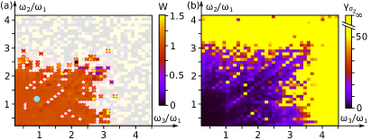
Figure 4: A trichromatically-driven qubit realization of the q-FTEP. (a) Topological index, $\nu$, obtained directly from Eq. (2) in the main text, as a function of $\omega_{2}$ and $\omega_{3}$. The white-shaded region indicates parameters where the effective spectral density in panel (b) exceeds $10$ and the simulation may not faithfully capture the system’s dynamics. (b) Effective spectral density for the model, $\gamma_{\sigma_{z}}$.

Here we provide data from numerical simulations of the 3-mode driven qubit model described in the main text. The simulations confirm that this system supports a topologically nontrivial regime characterized by the $3$-mode generalization of the invariant $\nu$ taking value $1$ (see main text for definition).

To demonstrate the nontrivial topology of the trichromatically-driven qubit, we simulate a qubit Hamiltonian similar to the dimensionally-reduced version of $\hat{H}_{\rm dr}(t)$ from the introduction. The Hamiltonian we consider features an additional fifth step where it takes value $\omega_{1}\sigma^{z}$, where $\sigma^{x,y,z}$ denote Pauli operators acting on the qubit states. We obtain the generalized Floquet eigenstates for the system by extending the Hilbert space to include the frequency space of modes $2$ and $3$ Ho et al. (1983); Luck et al. (1988); Casati et al. (1989); Blekher et al. (1992); Hatami et al. (2016); Else et al. (2020). To make this tractable, we truncated the Fourier harmonic indices of these modes to $N_{\rm c}=50$ each.

To investigate the extent of frequency localization in the system, we computed $\tilde{\sigma}_{z;N}(\omega)=\sum_{n=1}^{N}\frac{e^{in\omega T_{1}}}{\omega_{1}N}\langle\frac{\sigma_{z}(nT)+1}{2}\rangle$ with $N=65\hskip 1.5pt536$, and initial state ${|\!\uparrow\rangle}$. We then obtained the effective spectral density $\gamma_{\sigma_{z}}=(\int_{0}^{\omega_{1}}\!\!{\rm d}\omega\,|\tilde{\sigma}_{z;N}(\omega)|)^{2}/\int_{0}^{\omega_{1}}\!\!{\rm d\omega}\,|\tilde{\sigma}_{z;N}(\omega)|^{2}$. We expect $\gamma_{\sigma_{z}}$ serves as an equivalently valid measure of frequency localization to $\gamma$, while being more accessible for experimental measurement. For $\omega_{2},\omega_{3}\lesssim 3\omega_{1}$, we found $\gamma_{\sigma_{z}}<N_{c}$, indicating frequency localization.

We computed the topological invariant $\nu$ from the $3$-mode generalization of Eq. (2) from the main text, using the generalized micromotion operator for the system [see Fig. 4(a)]. The white color in Fig. 4(a) indicates the region where $\gamma_{\sigma_{z}}$ exceeds $10$, in which the simulation is not expected to accurately capture the system’s dynamics. In the localized region, $\nu$ exhibits a well-defined plateau where it takes value $1$, indicating that the system is in a topologically nontrivial regime.

References

- Vandersypen and Chuang (2005) L. M. K. Vandersypen and I. L. Chuang, Rev. Mod. Phys. 76, 1037 (2005).
- Bukov et al. (2015) M. Bukov, L. D’Alessio, and A. Polkovnikov, Adv. Phys. 64, 139 (2015).
- Weinberg et al. (2017) P. Weinberg, M. Bukov, L. D’Alessio, A. Polkovnikov, S. Vajna, and M. Kolodrubetz, Phys. Rep. 668, 1 (2017).
- Lindner et al. (2011) N. H. Lindner, G. Refael, and V. Galitski, Nat Phys 7, 490 (2011).
- Struck et al. (2012) J. Struck, C. Ölschläger, M. Weinberg, P. Hauke, J. Simonet, A. Eckardt, M. Lewenstein, K. Sengstock, and P. Windpassinger, Phys. Rev. Lett. 108, 225304 (2012).
- Wang et al. (2013) Y. H. Wang, H. Steinberg, P. Jarillo-Herrero, and N. Gedik, Science 342, 453 (2013).
- Jotzu et al. (2014) G. Jotzu, M. Messer, R. Desbuquois, M. Lebrat, T. Uehlinger, D. Greif, and T. Esslinger, Nature 515, 237 (2014).
- McIver et al. (2020) J. W. McIver, B. Schulte, F. U. Stein, T. Matsuyama, G. Jotzu, G. Meier, and A. Cavalleri, Nat. Phys. 16, 38 (2020).
- Viola and Lloyd (1998) L. Viola and S. Lloyd, Phys. Rev. Lett. 58, 2733 (1998).
- Viola et al. (1999) L. Viola, E. Knill, and S. Lloyd, Phys. Rev. Lett. 82, 2417 (1999).
- de Lange et al. (2010) G. de Lange, A. H. Wang, D. Risté, V. V. Dobrovitski, and R. Hanson, Science 330, 60 (2010).
- Dalibard et al. (2011) J. Dalibard, F. Gerbier, G. Juzeliunas, and P. Öhberg, Rev. Mod. Phys. 83, 1523 (2011).
- Struck et al. (2011) J. Struck, C. Ölschläger, R. Le Targat, P. Soltan-Panahi, A. Eckardt, M. Lewenstein, P. Windpassinger, and K. Sengstock, Science 333, 996 (2011).
- Goldman and Dalibard (2014) N. Goldman and J. Dalibard, Phys. Rev. X 4, 031027 (2014).
- Jiang et al. (2011) L. Jiang, T. Kitagawa, J. Alicea, A. R. Akhmerov, D. Pekker, G. Refael, J. I. Cirac, E. Demler, M. D. Lukin, and P. Zoller, Phys. Rev. Lett. 106, 220402 (2011).
- Rudner et al. (2013) M. S. Rudner, N. H. Lindner, E. Berg, and M. Levin, Phys. Rev. X 3, 031005 (2013).
- Nathan and Rudner (2015) F. Nathan and M. S. Rudner, New Journal of Physics 17, 125014 (2015).
- Khemani et al. (2016) V. Khemani, A. Lazarides, R. Moessner, and S. L. Sondhi, Phys. Rev. Lett. 116, 250401 (2016).
- von Keyserlingk C. W. and Sondhi (2016a) von Keyserlingk C. W. and S. L. Sondhi, Phys. Rev. B 93, 245145 (2016a).
- von Keyserlingk C. W. and Sondhi (2016b) von Keyserlingk C. W. and S. L. Sondhi, Phys. Rev. B 93, 245146 (2016b).
- Kitagawa et al. (2010) T. Kitagawa, E. Berg, M. Rudner, and E. Demler, Phys. Rev. B 82, 235114 (2010).
- Titum et al. (2016) P. Titum, E. Berg, M. S. Rudner, G. Refael, and N. H. Lindner, Phys. Rev. X 6, 021013 (2016).
- Nathan et al. (2017) F. Nathan, M. S. Rudner, N. H. Lindner, E. Berg, and G. Refael, Phys. Rev. Lett. 119, 186801 (2017).
- Nathan et al. (2019a) F. Nathan, D. Abanin, E. Berg, N. H. Lindner, and M. S. Rudner, Phys. Rev. B 99, 195133 (2019a).
- Wintersperger et al. (2020) K. Wintersperger, C. Braun, F. N. Ünal, A. Eckardt, M. D. Liberto, N. Goldman, I. Bloch, and M. Aidelsburger, Nat. Phys. 16, 1058 (2020).
- Sacha (2015) K. Sacha, Phys. Rev. A 91, 033617 (2015).
- Else et al. (2016) D. V. Else, B. Bauer, and C. Nayak, Phys. Rev. Lett. 117, 090402 (2016).
- Yao et al. (2017) N. Y. Yao, A. C. Potter, I.-D. Potirniche, and A. A. Vishwanath, Phys. Rev. Lett. 118, 030401 (2017).
- Zhang et al. (2017) J. Zhang, P. W. Hess, A. Kyprianidis, P. Becker, A. Lee, J. Smith, G. Pagano, I.-D. Potirniche, A. C. Potter, A. Vishwanath, N. Y. Yao, and C. Monroe, Nature 543, 217 (2017).
- Choi et al. (2017) S. Choi, J. Choi, R. Landig, G. Kucsko, H. Zhou, J. Isoya, F. Jelezko, S. Onoda, H. Sumiya, V. Khemani, C. Keyserlingk, N. Y. Yao, E. Demler, and M. D. Lukin, Nature 543, 221 (2017).
- Else et al. (2020) D. V. Else, W. W. Ho, and P. T. Dumitrescu, Phys. Rev. X 10, 021032 (2020).
- Ho et al. (1983) T.-S. Ho, S.-I. Chu, and J. V. Tietz, Chem. Phys. Lett. 96, 464 (1983).
- Luck et al. (1988) J. M. Luck, H. Orland, and U. Smilansky, J. Stat. Phys. 53, 551 (1988).
- Casati et al. (1989) G. Casati, I. Guarneri, and D. L. Shepelyansky, Phys. Rev. Lett. 62, 345 (1989).
- Blekher et al. (1992) P. M. Blekher, H. R. Jauslin, and J. L. Lebowitz, J. Stat. Phys. 68, 271 (1992).
- Hatami et al. (2016) H. Hatami, C. Danieli, J. D. Bodyfelt, and S. Flach, Phys. Rev. E 93, 062205 (2016).
- Kolodrubetz et al. (2018) M. H. Kolodrubetz, F. Nathan, S. Gazit, T. Morimoto, and J. E. Moore, Phys. Rev. Lett. 120, 150601 (2018).
- Martin et al. (2017) I. Martin, G. G. Refael, and B. Halperin, Phys. Rev. X 7, 041008 (2017).
- Nathan et al. (2019b) F. Nathan, I. Martin, and G. Refael, Phys. Rev. B 99, 094311 (2019b).
- (40) See Supplementary Online Material (SOM) for details.
- Shirley (1965) J. H. Shirley, Physical Review 138, B979 (1965).
- Ye et al. (2020) B. Ye, F. Machado, C. D. White, R. S. K. Mong, and N. Y. Yao, Phys. Rev. Lett. 125, 030601 (2020).
- (43) Each value of we probed was obtained by adding a small random number to a value generated by a different algorithm. Consequently, each sampled value of was incommensurate with (up to machine precision) for all but a measure-zero set of outcomes.
- Qi et al. (2008) X.-L. Qi, T. L. Hughes, and S.-C. Zhang, Phys. Rev. B 78, 195424 (2008).
- Vahala (2003) K. J. Vahala, Nature 424, 839 (2003).
- Long et al. (2021) D. M. Long, P. J. D. Crowley, and A. Chandran, Phys. Rev. Lett. 126, 106805 (2021).
- Leinonen (2017) M. Leinonen, On Various Irrationality Measures, Ph.D. thesis, University of Oulu (2017).
- Note (1) See, e.g., Ref. Leinonen (2017) for a review of irrationality measures.
- (49) A natural concern is that it is unnatural to introduce periodic boundary conditions along the () direction due to the constant tilt . However, when the Floquet states are localized in the -direction, we can arbitrarily modify the behavior at without affecting the topological properties for finite .
Supplementary Material